Optimal Monetary and Prudential Policies - bde.es · Prudential policy Proposition 4: A necessary...

Introduction Model Implications Extensions Conclusion

Optimal Monetary and Prudential Policies

Fabrice Collard, University of BernHarris Dellas, University of Bern

Behzad Diba, Georgetown UniversityOlivier Loisel, CREST

3rd Bank of Spain−World Bank Research Conference“Financing Growth: Levers, Boosters and Brakes”

Madrid, June 23, 2014

Collard, Dellas, Diba, and Loisel Optimal Monetary and Prudential Policies June 23, 2014 1 / 22


A forthcoming prudential policy

The recent crisis has highlighted the need for a policy ensuring financialstability.

The consensus [e.g. Bernanke (2011), IMF (2013)] is that it should be a newprudential policy (PP), rather than monetary policy (MP).

One key PP instrument will be bank capital requirements set conditionally onthe state of the economy [Basel Committee on Banking Supervision (2010)].



Contribution of the paper

This raises the issue of the interactions between

MP, i.e. interest-rate policy,PP, i.e. state-contingent capital-requirement policy.

Our goal is to develop a New Keynesian model with banks to study theseinteractions from a normative perspective.

The literature has recently proposed models that address this issue: e.g.,Angeloni and Faia (2013), Benes and Kumhof (2012), Christensen, Meh andMoran (2011).

We depart from this literature in two main ways:

by computing the jointly locally Ramsey-optimal policies,by linking the amount of risk to the type of credit.



Optimal simple rules vs. locally Ramsey-optimal policies

The literature gets jointly optimal simple rules:

the deviations of the policy instruments from their steady-statevalues are optimized within some parametric families of simple rules,

the steady-state value of capital requirements is not optimal.

We get jointly locally Ramsey-optimal policies, i.e. we get a state-contingent path for the two policy instruments that locally maximizesthe representative household’s ex ante utility.



Volume vs. type of credit

In the literature, the amount of risk is linked to the volume of credit (e.g.,through a systemic-risk externality in Christensen, Meh and Moran, 2011).

This link gives rise to a risk-taking channel of MP.

Our model illustrates another channel of interaction between MP and PP, bylinking the amount of risk to the type of credit.

Banks have an incentive to make socially undesirable risky loans, rather thansafe loans, because of a moral-hazard problem.

The two policies may not affect the same margins:

MP affects the volume but not necessarily the type of credit,PP affects both the volume and the type of credit.



Main results

We first develop a benchmark model, in which MP cannot affect the typeof credit.

This model implies a clear-cut optimal division of tasks between MP and PP:

PP should react only to shocks that affect banks’ risk-taking incentives,

in response to these shocks, MP should move opposite to PP in order tomitigate its macroeconomic effects [as envisaged by some policymakers andcommentators: Macklem (2011), Wolf (2012), Yellen (2010)].

We then consider two extensions to this model, one in which MP can affectthe type of credit.

These extensions can account for situations in which MP and PP should bothmove counter-cyclically.



Outline of the presentation

1 Introduction

2 Model

3 Implications

4 Extensions

5 Conclusion



Extending the New Keynesian model

Start from the basic New Keynesian model with capital, whose agents are

intermediate goods producers,final goods producers,households,a monetary authority.

There are two inefficiencies on the intermediate goods market:

monopolistic competition,price rigidity a la Calvo (1983),

which give a role to monetary policy.

Introduce, in turn, three additional types of agents:

capital goods producers (who have access to a risky technology),banks (which finance capital goods producers),a prudential authority (which imposes capital requirements on banks).



Capital goods producers I

Capital goods producers

buy unfurbished capital xt at the end of period t,furbish it between period t and period t + 1,sell this furbished capital kt+1 at the start of period t + 1.

They are perfectly competitive and owned by households.

They have access to a safe technology (S): kt+1 = xt ...

...and to a risky technology (R): kt+1 = θt exp(ηRt )xt , where

θt is a common (systemic) shock,θt = 0 with exogenous probability φt ,θt = 1 with exogenous probability 1− φt ,all realizations of ηR

t are positive,corr (θt , other shocks) = 0.



Capital goods producers II

At each period t, the timing of events is the following:1 all exogenous shocks are realized, except θt ,2 all agents observe these realizations and make their decisions,3 θt is realized.

R is inefficient in the sense that, for all realizations of φt and ηRt ,

(1− φt) exp(

ηRt

)≤ 1.

However, because of their limited liability, capital goods producers have anincentive to use R (“heads I win, tails you lose”): this is the first moral-hazard problem in the model.

To buy unfurbished capital, capital goods producers borrow from banks(which can monitor them) at the nominal interest rate R i

t with i ∈ {S , R},and those choosing R completely default on their loans when R fails.



Banks

Banks are perfectly competitive and owned by households.

They pay a tax (τ) on their profits.

They finance safe loans lSt and risky loans lRt by raising equity et and issuingdeposits dt , so that their balance-sheet identity is

lSt + lRt = et + dt .

Because of deposit insurance and their own limited liability, they have anincentive to make risky loans (again, “heads I win, tails you lose”).

This is the second moral-hazard problem in the model (as in the micro-banking literature, Van den Heuvel, 2008, Martinez-Miera and Suarez, 2012).

They can hide risky loans in their portfolio from the prudential authority upto an exogenous fraction γt of their safe loans.



Prudential authority

The prudential authority imposes a risk-weighted capital requirement:

et ≥ κt(

lSt + lRt

)+ κ max

{0, lRt − γt lSt

}.

This capital requirement enables it to tackle the second moral-hazardproblem: the higher banks’ capital et , the more banks internalizethe social cost of risk (as they have more “skin in the game”).

It optimally chooses κ high enough for lRt ≤ γt lSt in equilibrium.

This is because risky loans are socially undesirable, as

R is inefficient on average over θt ,θt is independent of the other shocks,households are risk-averse.



Two preliminary results

Proposition 1: There are no equilibria with 0 < lRt < γt lSt .

This is because banks’ limited liability make their expected excess returnconvex in the volume of their risky loans.

Proposition 2: In equilibrium, the capital constraint is binding:

et = κt(

lSt + lRt

).

This is because the tax on banks’ profits makes them prefer debt finance toequity finance.



Prudential policy

Proposition 4: A necessary and sufficient condition for existence of anequilibrium with lRt = 0 is κt ≥ κ∗t (where κ∗t is a function of shocks, madeexplicit in the paper).

Starting from a situation in which all banks are at the safe corner, settingκt ≥ κ∗t deters each bank from going to the risky corner by making itsufficiently internalize the social cost of risk.

This threshold value κ∗t is increasing in

the probability of success of the risky technology 1− φt ,the productivity of the risky technology conditionally on its success ηR

t ,the maximum ratio of risky to safe loans γt ,

as an increase in 1− φt , ηRt , or γt raises banks’ risk-taking incentives.



Monetary policy

The MP instrument is the risk-free deposit rate RDt .

κ∗t does not depend on RDt : there is no risk-taking channel of MP, or

equivalently MP is ineffective in ensuring financial stability.

This is because, in our benchmark model with perfect competition andconstant returns, RD

t does not affect the spread between RRt and RS

t ,and hence does not affect banks’ risk-taking incentives.

Let (RD∗τ )τ≥0 denote the MP that is Ramsey-optimal when PP is (κ∗τ)τ≥0.



Jointly locally Ramsey-optimal policies

Proposition 5: If the right derivative of welfare with respect to κt at(RD

τ , κτ)τ≥0 = (RD∗τ , κ∗τ)τ≥0 is strictly negative for all t ≥ 0, then the

policy (RDτ , κτ)τ≥0 = (RD∗

τ , κ∗τ)τ≥0 is locally Ramsey-optimal.

Setting κt just below κ∗t is not optimal, because it triggers a discontinuousincrease in the amount of (inefficient) risk taken by banks.

Setting κt just above κ∗t is not optimal, because it has a negative first-orderwelfare effect that cannot be offset by any change in RD

t around its optimalsteady-state value RD∗ (as this change would have a zero first-order effect).

We check numerically, using Levin and Lopez-Salido’s (2004) “Get Ramsey”program, that the right derivative of welfare with respect to κt at(RD∗

τ , κ∗τ)τ≥0 is strictly negative.

This is because increasing κt from κ∗t decreases the capital stock, which isalready inefficiently low due to the monopoly and tax distortions.



Numerical simulations

We calibrate the model and consider two alternative PPs:

the optimal PP κt = κ∗t , with a steady-state value κ∗ = 0.10,the passive PP κt = 0.12, which also ensures lRt = 0.

For each PP, we compute the optimal MP using Get Ramsey.

There are two types of shocks:1 shocks that do not affect banks’ risk-taking incentives: ηf

t , Gt ,2 shocks that affect banks’ risk-taking incentives: ηR

t , γt , φt , Ψt .

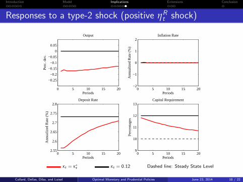
Following type-1 shocks, optimal PP does not move, while optimal MPmoves in a standard way.

Following type-2 shocks, optimal MP moves opposite to optimal PP in orderto mitigate its macroeconomic effects [as envisaged by some policymakersand commentators: Macklem (2011), Wolf (2012), Yellen (2010)].



Responses to a type-2 shock (positive ηRt shock)

0 5 10 15 20

−0.25

−0.2

−0.15

−0.1

−0.05

0

0.05

Output

Periods

Per

c. d

ev.

0 5 10 15 20−2

−1

0

1

2Inflation Rate

Periods

Ann

ualiz

ed R

ate

(%)

0 5 10 15 202.55

2.6

2.65

2.7

2.75

2.8Deposit Rate

Periods

Ann

ualiz

ed R

ate

(%)

0 5 10 15 209

10

11

12

13Capital Requirement

Periods

Per

cent

ages

κt = κ∗t κt = 0.12 Dashed line: Steady State Level



Two extensions

In our benchmark model, optimal MP and optimal PP never move in thesame direction.

We consider two extensions to this model, which can make optimal MP andoptimal PP move in the same (counter-cyclical) direction.

Extension 1: we introduce productivity shocks on S that are positivelycorrelated with productivity shocks on R.

Extension 2: we introduce an externality by assuming that banks’ marginalmonitoring cost is increasing in the aggregate volume of loans [as in Hachem(2010)]: log(Ψt) = log(Ψ) + $[log(lSt )− log(lS )].

Unlike Extension 1, Extension 2 enables MP to affect the type of credit, i.e.it gives rise to a risk-taking channel of MP, or equivalently it makes MPeffective in ensuring financial stability.



Extension 1: responses to a positive ηRt shock

0 5 10 15 200

0.1

0.2

0.3

0.4

0.5Output

Periods

Per

c. d

ev.

0 5 10 15 20−2

−1

0

1

2Inflation Rate

Periods

Ann

ualiz

ed R

ate

(%)

0 5 10 15 202.6

2.8

3

3.2

3.4Deposit Rate

Periods

Ann

ualiz

ed R

ate

(%)

0 5 10 15 2010

10.5

11

11.5Capital Requirement

Periods

Per

cent

ages

corr(ηRt , ηS

t ) = 0.25 corr(ηRt , ηS

t ) = 0.50 corr(ηRt , ηS

t ) = 0.75

Thin Dashed Line: Steady State Level



Extension 2: responses to a positive ηft shock

0 5 10 15 20

0.4

0.6

0.8

1

1.2

Output

Periods

Per

c. d

ev.

0 5 10 15 20−2

−1

0

1

2Inflation Rate

Periods

Ann

ualiz

ed R

ate

(%)

0 5 10 15 20

2.7

2.75

2.8

2.85

2.9

2.95Deposit Rate

Periods

Ann

ualiz

ed R

ate

(%)

0 5 10 15 209.9

9.95

10

10.05

10.1

10.15

Capital Requirement

Periods

Per

cent

ages

$ = 0 $ = 1 $ = 5 Thin Dashed Line: Steady State Level



Conclusion

We develop a New Keynesian model with banks to study the interactionsbetween MP and PP from a normative perspective.

We depart from the literature in two main ways:

by linking the amount of risk to the type of credit,by computing the jointly locally Ramsey-optimal policies.

We obtain a clear-cut optimal division of tasks between MP and PP:

PP should react only to shocks that affect banks’ risk-taking incentives,MP should react to all shocks and, for some shocks, only to their effects onthe PP instrument.

We can account for situations in which

MP and PP should move opposite to each other,MP and PP should move in the same (counter-cyclical) direction.


Appendix

Addressing commentators’ and policymakers’ concerns

Wolf (2012): “How, in practice, will policies aimed at securing financialstability interact with monetary policy? Consider, for example, the possibilitythat the committee charged with the former is trying to cool lending in, say,the property sector when the committee charged with the latter is seeking toheat it up in the economy. They could find themselves operating incontradiction.”

Yellen (2010): “[W]e must strive to avoid situations in which macro-prudential and monetary policies are working at cross-purposes, given thatmacroprudential policies affect macroeconomic performance and thatmonetary policy may affect risk-taking incentives.”

Collard, Dellas, Diba, and Loisel Optimal Monetary and Prudential Policies June 23, 2014 A1 / A14

Appendix

Our modeling contribution

The moral-hazard problem that gives banks an incentive to make sociallyundesirable risky loans is due to limited liability and deposit insurance, as in abranch of the micro-banking literature.

Van den Heuvel (2008) introduces this kind of moral-hazard problem into ageneral-equilibrium (GE) model with

no systemic risk,no aggregate shocks.

Martinez-Miera and Suarez (2012) introduce it into a GE model with

systemic risk,no aggregate shocks.

We introduce it into a GE model with

systemic risk,aggregate shocks,sticky prices,monetary policy.


Appendix

Intermediate and final goods producers

Intermediate goods producers are monopolistically competitive and face aprice rigidity a la Calvo (1983).

The production function of intermediate goods producer j is

yt(j) = ht(j)1−νkt(j)

ν exp(

ηft

).

Final goods producers are perfectly competitive.

Their production function is

yt =

(∫ 1

0yt(j)

σ−1σ dj

) σσ−1

.


Appendix

Households’ optimization problem

Households choose (ct , ht , dt , st , kt , it , xt)t≥0 to maximize

E0

∞

∑t=0

βt

[log(ct)−

h1+χt

1 + χ

]subject to

the budget constraint ct + dt + qbt st + qtkt + it = wtht+1+RD

t−1Πt

dt−1 + st−1ωbt + ztkt + qxt xt + (ωk

t + ωft − τh

t ),

the law of motion of capital xt = (1− δ)kt + it .


Appendix

Capital goods producers II (more detailed version)

At each period t, the timing of events is the following:1 all exogenous shocks are realized, except θt ,2 all agents observe these realizations and make their decisions,3 θt is realized.

R is inefficient in the sense that, for all realizations of φt , ηRt and Ψt ,

(1− φt) exp(

ηRt

)≤ 1−Ψt ,

where Ψt is the marginal resource cost of monitoring capital goods producers.

However, because of their limited liability, capital goods producers have anincentive to use R (“heads I win, tails you lose”): this is the first moral-hazard problem in the model.


Appendix

Capital goods producers III

Capital goods producers need to get funds to buy unfurbished capital.

The only agents that have the skills to monitor them (and thus that cansolve the first moral-hazard problem) are banks.

Therefore, they get funds from banks to buy unfurbished capital.

We consider loan contracts between capital goods producers and banks.

That is, the capital goods producers choosing technology i ∈ {S , R} borrowthe funds they need at the nominal interest rate R i

t ...

...and those choosing R completely default on their loans when R fails.


Appendix

Capital goods producers IV

A producer i using technology S chooses xt (i) to maximize

βEt

{λt+1

λt

[qt+1xt (i)−

1 + RSt

Πt+1qxt xt (i)

]},

where λt is households’ marginal utility of consumption at date t.

A producer i using technology R chooses xt (i) to maximize

(1− φt)βEt

{λt+1

λt

[qt+1 exp(ηR

t )xt (i)−1 + RR

t

Πt+1qxt xt (i)

] ∣∣∣∣∣θt = 1

}.


Appendix

Banks II

Banks only need to monitor the capital goods producers who borrow at thelower rate.

This lower rate is RSt .

Indeed, if we had RRt < RS

t , then funding safe projects would strictlydominate funding risky projects as it would

pay more even when R is a success,incur no monitoring cost.

So banks only monitor the capital goods producers who borrow at rate RSt , in

order to check that they use S.

Banks last for only two periods, so that there is no durable relationshipbetween banks and capital goods producers.


Appendix

Banks III

The representative bank chooses et , dt , lRt and lSt to maximize

Et

{β

λt+1 (1− τ)ωbt+1

λt

}− et − (1− τ)Ψt lSt ,

where

ωbt+1 = max

{0,

1 + RSt

Πt+1lSt + θt

1 + RRt

Πt+1lRt −

1 + RDt

Πt+1dt

},

subject to

lSt + lRt = et + dt ,

lRt ≤ γt lSt ,

et ≥ κt(lSt + lRt

).


Appendix

Gvt’s budget constraint and goods market clearing cdt

The government’s budget constraint is

τht = Gt +∫ 1

0

{ζt(j)− τ[ωb

t (j) + Ψt lSt (j)]}

dj ,

where losses imposed by bank j on the deposit insurance fund are ζt(j) =

max

{0,

1 + RDt−1

Πtdt−1(j)−

1 + RSt−1

ΠtlSt−1(j)− θt−1

1 + RRt−1

ΠtlRt−1(j)

}.

The goods market clearing condition is

ct + it + Gt + Ψt lSt = yt .


Appendix

Prudential-policy rule

Proposition 6: Under the PP rule

κt =1− φt

φt

γt

1 + γt

RRt − RS

t

1 + RDt

+1

φt

γt

1 + γtΨt −

RSt − RD

t

1 + RDt

,

there exists a unique equilibrium and, at this equilibrium, lRt = 0 andκt = κ∗t .

On the right-hand side of this feedback rule, for an individual bank movingfrom the safe to the risky corner,

the first two terms represent the benefit of this move: pocketing RRt − RS

t ifrisky projects succeed and saving monitoring costs Ψt ,

the third term represents the opportunity cost of this move: losing RSt − RD

tif risky projects fail.


Appendix

Calibration

Parameter Description ValuePreferences

β Discount factor 0.993χ Inverse of labor supply elasticity 1.000

Technologyν Capital elasticity 0.300σ Elasticity of substitution 7.000δ Depreciation rate 0.025

Nominal rigiditiesα Price stickiness 0.667

Banking (steady state)τ Tax rate 0.023κ∗ Capital requirement 0.100Ψ Marginal monitoring cost 0.006φ Failure probability 0.029γ Maximal risky/safe loans ratio 0.427exp(ηR ) Productivity of the risky technology 1.005

Shock processesρ Persistence 0.950


Appendix

Responses to a type-1 shock (positive ηft shock)

0 5 10 15 20

0.7

0.8

0.9

1

1.1

1.2

1.3

Output

Periods

Per

c. d

ev.

0 5 10 15 20−2

−1

0

1

2Inflation Rate

Periods

Ann

ualiz

ed R

ate

(%)

0 5 10 15 20

2.7

2.75

2.8

2.85

2.9

2.95Deposit Rate

Periods

Ann

ualiz

ed R

ate

(%)

0 5 10 15 209

10

11

12

13Capital Requirement

Periods

Per

cent

ages

κt = κ∗t κt = 0.12 Dashed line: Steady State Level


Appendix

Justification of policy-induced distortions

There are two policy-induced distortions in the model:

deposit insurance, which gives rise to banks’ risk-taking incentives,the tax on banks’ profits, which makes the capital requirement binding.

We assume that they are not decided by the mon. and prud. authorities.

These distortions are prevalent in many countries and do not seem to belikely to be removed any time soon.

We could probably justify deposit insurance by introducing the possibility ofbank runs, at the cost of greater complexity.

When the tax is arbitrarily small,

all our analytical results (from Proposition 1 to Proposition 6) still hold,the condition stated in Prop. 5 (the “if” part of this prop.) may not be met,our model is equivalent, at the first order, to a model with no tax and withdeposits in the utility function with an arbitrarily small weight.


Optimal Monetary and Prudential Policies - bde.es · Prudential policy Proposition 4: A necessary...

Documents

Transcript of Optimal Monetary and Prudential Policies - bde.es · Prudential policy Proposition 4: A necessary...