Optimal investment strategies using multi-property ...
38
University of Central Florida University of Central Florida STARS STARS HIM 1990-2015 2012 Optimal investment strategies using multi-property commercial Optimal investment strategies using multi-property commercial real estate analysis of pre/post housing bubble real estate analysis of pre/post housing bubble Kyle Kundiger University of Central Florida Part of the Finance Commons Find similar works at: https://stars.library.ucf.edu/honorstheses1990-2015 University of Central Florida Libraries http://library.ucf.edu This Open Access is brought to you for free and open access by STARS. It has been accepted for inclusion in HIM 1990-2015 by an authorized administrator of STARS. For more information, please contact [email protected]. Recommended Citation Recommended Citation Kundiger, Kyle, "Optimal investment strategies using multi-property commercial real estate analysis of pre/post housing bubble" (2012). HIM 1990-2015. 1360. https://stars.library.ucf.edu/honorstheses1990-2015/1360
Transcript of Optimal investment strategies using multi-property ...

University of Central Florida University of Central Florida
STARS STARS
HIM 1990-2015
2012
Optimal investment strategies using multi-property commercial Optimal investment strategies using multi-property commercial
real estate analysis of pre/post housing bubble real estate analysis of pre/post housing bubble
Kyle Kundiger University of Central Florida
Part of the Finance Commons
Find similar works at: https://stars.library.ucf.edu/honorstheses1990-2015
University of Central Florida Libraries http://library.ucf.edu
This Open Access is brought to you for free and open access by STARS. It has been accepted for inclusion in HIM
1990-2015 by an authorized administrator of STARS. For more information, please contact [email protected].
Recommended Citation Recommended Citation Kundiger, Kyle, "Optimal investment strategies using multi-property commercial real estate analysis of pre/post housing bubble" (2012). HIM 1990-2015. 1360. https://stars.library.ucf.edu/honorstheses1990-2015/1360
OPTIMAL INVESTMENT STRATEGIES USING MULTI-PROPERTY
COMMERCIAL REAL ESTATE: ANALYSIS OF PRE/POST HOUSING
BUBBLE
by
KYLE R. KUNDIGER
A thesis submitted in partial fulfillment of the requirements
for the Honors in the Major Program in Business Finance
in the College of Business Administration
and in The Burnett Honors College
at the University of Central Florida
Orlando, Florida
Fall Term 2012
Thesis Chair: Dr. Melissa Frye

ii
ABSTRACT
This paper analyzes theperformance of five commercial real estate property types (office,
retail, industrial, apartment, and hotel) between 2000 and 2012 to determine the U.S. housing
crisis’simpact on Real Estate investing. Under the concept of Modern Portfolio Theory, the data
was analyzed using investment analysis programs to determine correlation, risk/return
characteristics, and trade-offs (Sharpe ratio) as well as the optimal allocation among the
individual property types. In light of the results, each property type plays a different role in
investment strategies in various economic cycles. Some assets are attractive solely based
onpotential return, or risk for return tradeoffs; however, through diversification, other property
types play valuable roles in hedging risk on investors’ target returns.

iii
AKNOWLEDGEMENTS
I express sincere thanks and gratitude to my committee members, who have been gracious
enough to enable this project with their guidance, knowledge, and experience. Special thanks go to
my thesis chair, Dr. Melissa Frye, for her patience and willingness to help witheverything that came
up along the way. Without her, this paper would never have become anything close to a realization,
and I am truly grateful. Also, thank you to my in-department committee member, Dr. Yoon Choi, for
his help with data analysis and support. Thank you, also to my out-of-department committee
member, Dr. Joshua Harris and Dr. Cameron Ford, for their guidance in translating my ideas into a
reality. And lastly, thank you to Ashley Pruitt, for her never-ending support throughout the entire
research and thesis writing process.

iv
TABLE OF CONTENTS
INTRODUCTION ............................................................................................................................................. 1
MODERN PORTFOLIO THEORY ...................................................................................................................... 2
STOCKS VS REAL ESTATE ............................................................................................................................... 4
PROPEPRTY TYPE COMPARISONS ................................................................................................................. 6
Housing Bubble ......................................................................................................................................... 8
HYPOTHESIS ................................................................................................................................................ 10
DATA ........................................................................................................................................................... 11
Result ...................................................................................................................................................... 11
Individual Property Type Comparisons: 2000 to 2012............................................................................ 11
Correlation .............................................................................................................................................. 14
Efficient Frontier ..................................................................................................................................... 16
Risk and Return ....................................................................................................................................... 18
Alternative Allocation Methods .............................................................................................................. 19
Period 2: Sub-Periods .............................................................................................................................. 22
Period 2-1 ............................................................................................................................................ 23
Period 2-2 ............................................................................................................................................ 24
Period 2-3 ............................................................................................................................................ 25
Period 2-4 ............................................................................................................................................ 27
Summary ............................................................................................................................................. 27
CONCLUSION ............................................................................................................................................... 29
REFERENCES ................................................................................................................................................ 30

v
LIST OF FIGURES
Figure 1: Quarter-annual property returns and S&P 500 returns: (2000-2012) .......................................... 12
Figure 2: Comparative efficient frontiers (Period 1 & Period 2) ................................................................ 17
Figure 3: Efficient frontier & 100% allocation of individual property types & equal weights (Period 1) . 20
Figure 4: Efficient frontier & 100% allocation of individual property types & equal weights (Period 2) vs.
(Period 1) .................................................................................................................................................... 20
Figure 5: Efficient frontiers (Period 1, Period 2 & Period 2 sub-set periods) ............................................. 22

vi
LIST OF TABLES
Table 1: Summary of individual property type risk, return and Sharpe ratio (Period 1) & (Period 2) ....... 14
Table 2: Correlation Matrix (Period 1) & (Period 2) .................................................................................. 15
Table 3: Allocation weights and risk/return range (Period 1) ..................................................................... 18
Table 4: Allocation weights and risk/return range (Period 2) ..................................................................... 19
Table 5: Alternative Portfolios (Period 1) & (Period 2) ............................................................................. 21
Table 6: Summary of individual property type risk, return and Sharpe ratio (Period 2-1;2-2;2-3;2-4) ...... 23
Table 7: Allocation weights and risk/return range (Period 2-1) ................................................................. 24
Table 8: Allocation weights and risk/return range (Period 2-2) ................................................................. 25
Table 9: Allocation weights and risk/return range (Period 2-3) ................................................................. 25
Table 10: Allocation weights and risk/return range (Period 2-4) ............................................................... 26

1
INTRODUCTION
In portfolio optimization, investors seek an allocation of assets providing the lowest risk
for return. As such, there are a variety of assets to choose from including stocks, bonds, to even
real estate. Then within Real Estate, investors must decide which specific property types to mix
in their investment portfolio. Modern Portfolio Theory states that investors analyze assets’
expected return, standard deviation, and correlation characteristics. This allows for investors to
explore diversification strategies between the assets, thereby determining what mix of assets will
achieve a specific target return at minimized risk. Asset mixtures vary during various economic
cycles, and many times it’s not necessarily a question of what to invest in, but what not to invest
in. As such, investors are continuously adapting to changing economic conditions and continue
to attempt to capitalize on market opportunities.

2
MODERN PORTFOLIO THEORY
Modern Portfolio Theory; shortly put, is the financial theory involving rational, risk
adverse investors allocating assets within a portfolio to achieve the optimal asset combination.
First introduced by Markowitz and Sharpe (1952) it was conceptualized that through
diversification within a portfolio, an investor could achieve higher levels of return through
certain asset combinations. According to Lee and Stevenson (2005), each asset's performance
capability is gauged by risk and return characteristics. These are measured by its mean and
standard deviation (variation), and its portfolio risk compares its correlation with alternative
assets. By applying these parameters, an investor will find the optimal combination of assets
offering the lowest level of risk for any target level of expected return or alternatively
determining the highest return for a certain level of risk, which is the process known as mean-
variance analysis (Cheng, Lin, Liu and Zhang, 2011). Postulated as an investment theory
encompassing different asset types, it applies to investments running from stocks, bonds, to real
estate.
Assets that are part of a MPT constructed portfolio can achieve higher returns for lower
risk than if considered individually. This is explained by the levels of correlation between the
different asset types. According to Cheng, Lin, Liu and Zhang, (2011) when the different
individual asset types are paired in a MPT constructed portfolio, this lowers their degrees of
correlation, and enlarges the likelihood of higher returns. If two asset types are completely
independent of one another, meaning none of the same variables affect them both, the correlation
would equal zero. As long as the assets are not perfectly correlated, an investor can benefit from
diversification.

3
Unsystematic risk is a risk arising from a factor unrelated to the market or the system
(Penny, 1982). This risk applies to a specific industry or firm; thus, it can be eradicated using
portfolio diversification. If it was considered systematic risk, also known as market risk, then
regardless of any combination of assets, this risk will still exist. It affects the entire market,
including all the industries within it, which in turn means that the goal of diversification is to
allocate enough assets so that only systematic risk remains within the portfolio. According to
Black (2004), by combining 30 stocks in a portfolio, the variance of the stock is diminished and
almost all unsystematic risk (diversifiable risk) is eliminated. Consequently, diversification is an
effective hedge against risk, and is beneficial when applied to MPT.
However effective, MPT contains limitations in its application to Real Estate. First, MPT
predicts normal distributed investment returns, which have been proven unrealistic in real estate.
More so, it has been deemed more effective to describe the results based on a stable infinite
variance skewed distribution, rather than a normal distribution (Sivitandies, 1998). Second, with
large numbers of investors, results have been inconsistent with MPT's assumption of controlled
focus groups. Even with those limitations, MPT is still an effective tool in determining optimal
allocation strategies in real estate, and is continually utilized by investors.

4
STOCKS VS REAL ESTATE
In real estate there are two types of investments, REITs, which are publicly traded real
estate securities, and private real estate, which are actual tangible properties. Between the two,
however, private real estate has been deemed more beneficial in terms of portfolio
diversification. This is explained by the correlation between the assets. The more directly an
asset is affected by a change in another, either positive or negative, the higher the correlation
between the two. According to Black (2004), when comparing the NAREIT Index and the
Russell 2000 Index (a small capitalization index) there was a high positive correlation of (.722).
However, when computing correlation between the NCREIF (a private real estate index based on
appraisal values and transactions) and the S&P 500, there was conversely a low correlation of
(.0523) (Black, 2004). The lower correlation between private real estate and the stock index
indicates that private real estate and stocks are mixed in an investment portfolio, investors
benefit from diversification.
When considering the optimal real estate allocation, the time frame plays a key factor. In
the long-term, research has shown that private real estate is considered a more worthwhile
investment. Fugazza, Guidolin and Nicodanna (2007), concluded that for a one-year time frame
the optimal real estate allocation was 9%; however, a ten-year time frame had an optimal real
estate allocation of 44%. Thus, over time real estate becomes increasingly attractive. This is
explained by the positive relationship real estate has with the investment horizon. Real estate is
deemed an illiquid asset in comparison to stocks and bonds. Hence, it is arguable that the longer
you plan on holding onto direct real estate, the larger its profit potential.

5
There are a variety of factors separating private real estate from securities, with one main
difference being efficiency. The stock market is considered efficient, investors have access to
individual stock prices through indexes such as the S&P 500. Within the stock market, prices and
market value are generally in equilibrium. Information on the market is widely available, so
either through buying or selling securities, investors bring the security price to equilibrium
almost immediately. Stocks are easily applied to MPT as the investment allocation system
assumes market efficiency, which the stock market experiences. Real estate property returns
however are more difficult to gauge. Unlike the stock market, real estate investors must consider
factors such as financial and operating leverage, location, leasing terms, and tenant mixtures to
measure unsystematic (diversifiable) risk in the real estate market. (Viezer 2000)
The private real estate market, by its very nature, is inefficient. Lin and Vandell (2007)
note that private real estate is considered a heterogeneous asset, and is plagued by market
uncertainty. Perhaps the most efficient gauge of private real estate values is the NCRIEF
database (private real estate index based on appraisal data and transaction costs), which
researchers have relied heavily on for information in the real estate markets. NCREIF only
releases quarterly returns, as opposed to the S&P 500 reporting daily returns. Only every quarter
can the real estate market essentially "fix itself" and put prices in equilibrium; therefore, it's
lagged in comparison to the stock market. Penny (1982) suggests that the general uniqueness of
properties, lower transactions, and real estate market differences also contributes to the difficulty
of pricing in the private real estate market.

6
PROPEPRTY TYPE COMPARISONS
Once a portfolio manager decides the optimal allocation of real estate to a mixed asset
portfolio, they then must decide how to diversify between the different property types and
geographical locations. Between the two, however, Petersen and Singh (2003), concluded that
property type diversification gives higher risk-adjusted returns as compared to geographical
diversification. Risk-adjusted returns are based on a reduction of nonsystematic risk. Overall,
there are five types of commercial property types generally recognized in the academic literature:
hotel, apartment, retail, industrial and office. Using MPT, investors construct the efficient
frontier to determine how much to distribute to each. Stephen and Simon (2005), Mueller and
Laposa (1995) suggest that returns for each, however, vary depending on different time periods
experiencing different economic cycles.
Mueller and Laposa, (1995) state that NCREIF returns data can be segmented into
different periods based on three indicators: GDP growth, total returns, and capital appreciation.
By separating the sub-periods, investors are able to construct time-period specific efficient
frontiers. Thus, investors determine the optimal allocation for each period, and portfolio weights
to different property types may vary. Those weights are determined by standard deviation,
expected return, and correlation. Once all three are determined, investors can plot the efficient
frontier (Petersen & Singh, 2003).
Petersen and Singh (2003) calculated risk, return, and adjusted-risk returns for each of the
five property types over a 20-year period, 1982-2001. During that period, apartments were the
most attractive investment with annualized returns of 10.15 percent. Apartments were followed

7
by industrial, retail, hotel, and office, implying office properties held the lowest returns, and
were thus least profitable. When considering volatility, hotels and office properties recorded the
highest standard deviations, suggesting they were the riskiest in terms of total risk. Conversely,
industrial, retail and apartment had lower standard deviations, concluding apartments were
associated with the least risk of the group. Lastly, apartments ranked the highest in terms of the
Sharpe ratio. The Sharpe ratio is essentially a measure of the unit of return you receive for every
unit of risk. Office properties, contrarily calculated a negative ratio. Hotels, retail, and industrial
each had relatively low, yet positive Sharpe ratios.
By developing a cross correlation matrix, Petersen and Singh (2003) also show the level
of correlation between the property types between 1982 and 2001. Hotel and retail had the lowest
correlation, meaning in terms of strict diversification, they were the most attractive combination.
Office and industrial properties, however, had the highest correlation, suggesting there were no
(or very little) diversification benefits between the two. Excluding hotels, the correlations
between the retail, office, industrial, and apartment sectors were all relatively high. These
correlations ranged from the lowest, between retail and apartment (0.61%) to the highest
correlation, between industrial and office 96 percent. Thus, from a diversification perspective,
hotels offer the most potential benefit between any one of the other property types, considering
none of hotel's correlations with any of the other property types rose over 50 percent. This
information allows an investor to construct the efficient frontier.
Petersen and Singh (2003) also show that between the years of 1982 and 2001, the
maximum risk-return portfolio had 100% weight on apartments, with a return of 4.95% and a

8
risk of 2.50%. At the minimum variance, the optimal portfolio consisted of 41% apartments,
44% retail, and 15% in hotels. That minimum risk point on the efficient frontier boasted a 4.47%
return accompanied by 2.25% of risk. Risk-adverse investors would suggestively benefit by
diversifying the portfolio beyond apartments, with hotels and retail. Less risk-adverse investors
would benefit from their portfolios consisting of mostly apartments and only a small percentage
in hotels and retail. Also, at no point on the efficient frontier did industrial and office properties
appear in the optimal allocation.
Contrary to Petersen and Singh (2003), Stephen and Simon (2005), analyzed returns
between four property types: retail, R&D, office, and warehouses between 1978 and 1988, they
determined that office properties were among the most profitable. These profitable office returns
contrast starkly with office returns between 1982 and 2001, as office properties were not
weighted in the efficient frontier. This exemplifies that no time invariant optimal portfolio
allocation strategy exists. Investors must adjust their allocation strategies during different
economic cycles. The U.S. housing bubble of 2006 is a prime example of this as detailed below.
Housing Bubble
During the early 2000's the U.S. housing market experienced rapid increases in home
pricing up until late 2005/early 2006, when home prices peaked and then essentially freefell
downward, thus creating a housing crisis. This process is known as the bursting of a housing
bubble. A housing bubble is theoretically described as a deviation of private real estate growth
from its normal rudiments (Lai & Van Order, 2010). Bubbles are caused by a variety of factors,
ranging from low interest rates, deregulation, easily accessible credit (subprime loans), and
9
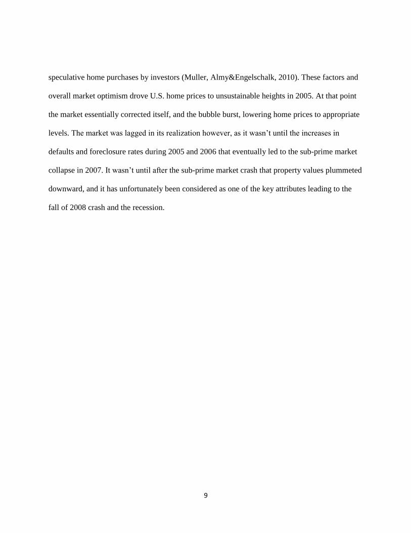
speculative home purchases by investors (Muller, Almy&Engelschalk, 2010). These factors and
overall market optimism drove U.S. home prices to unsustainable heights in 2005. At that point
the market essentially corrected itself, and the bubble burst, lowering home prices to appropriate
levels. The market was lagged in its realization however, as it wasn’t until the increases in
defaults and foreclosure rates during 2005 and 2006 that eventually led to the sub-prime market
collapse in 2007. It wasn’t until after the sub-prime market crash that property values plummeted
downward, and it has unfortunately been considered as one of the key attributes leading to the
fall of 2008 crash and the recession.

10
HYPOTHESIS
MPT plays a pivotal role in real estate investing, from determining how much of an
investment portfolio to dedicate to real estate; and specifically, choosing which real estate
property types to invest in. In this paper, I focus on the diversification within real estate by
specifically looking at the optimal asset allocation strategy to the various real estate property
types.
Prior research suggest that both apartments (Petersen and Singh, 2003) and office
properties (Stephen and Simon, 2005) have played important roles in real estate allocation
decisions. However, these studies relied on data prior to the house market crisis. Thus, I plan to
explore differences in optimization strategies in the pre-crisis period and the post-crisis period. I
expect to find that post-crisis, there will be a greater weight invested in apartments, due to the
rapid increase in foreclosures post-housing bubble. I also believe that hotels will become a less
attractive investment, since tourism has been negatively affected by the recession.
Furthermore,that the sub-prime market crash and the market crash of 2008 will have large
impacts on portfolio optimization strategies.

11
DATA
This study concentrates on quarterly-annual commercial property returns provided by the
NCREIF index from 2000 to 2012. The NCREIF index (national center of real estate investment
fiduciaries) releases quarter-annual returns for commercial property acquired in the private sector
for the sole purpose of investing. These properties in question were acquired from tax-exempt
institutional investors and then held in a fiduciary environment. In purpose of this study, quarter-
annual returns produced by NCRIEF, between 2000 and 2012 were analyzed.
Result
The analysis begins by illustrating the volatility of property returns between 2000 and
2012, followed by analysis on the comparative risk and return characteristics of each individual
commercial property type before and after the housing crisis. Correlation matrixes are produced
to show the possibility of diversification benefits between the property types. Time-period-
specific efficient frontiers are then constructed using risk and return rates, and in addition,
covariance data. Also plotted are alternative weight allocations in comparison to the efficient
frontiers. Then given the volatility of Period 2’s returns, sub-set efficient frontiers are also
created to demonstrate the differences in investment decisions within the separate time periods.
Individual Property Type Comparisons: 2000 to 2012
Between 2000 and 2012, there are many economic factors driving property return/risk
characteristics. From 2000 to 2005 Q2 property values rose to historical heights, while peaking
in Quarter 2, 2005; however, after peaking the market began showing signs of volatility with
increasing foreclosures and defaults. The sub-prime market collapsed in 2007 leading home

12
prices to catapult downward until crashing in the fall of 2008. Property returns remained
negative until 2010, when property values began slowly rising again resulting in positive returns.
Figure 1 illustrates the volatility of quarter-annual Real Estate returns between 2000 and 2012
and the S&P 500 quarter-annual returns.
Figure 1: Quarter-annual property returns and S&P 500 returns: (2000-2012)
Most noticeably in Figure 1 is the starkness of the S&P 500’s inflection points. Overall,
the S&P 500 appears to lack consistency and produced mostly inferior returns as opposed to real
estate; however, during the 2008 Q3 crash, excluding retail, the S&P 500 was less affected and
actually outperformed the alternative property types. Of the property types, hotels most
noticeably, appear to experience the highest volatility from 2000 to 2012 with stark increases and
decreases as shown in Figure 3. In Quarter 3 of 2001, for instance, hotel returns dropped
-0.15
-0.1
-0.05
0
0.05
0.1
Qtr 1 00 Qtr 1 02 Qtr 1 04 Qtr 1 06 Qtr 1 08 Qtr 1 10 Qtr 1 12
Exp
ect
ed
Re
turn
(M
ean
)
Date
Office
Industrial
Retail
Apartment
Hotel
S&P 500

13
substantially, most presumably because of the terrorist acts on 9/11. Also, during the crash in
2008, hotels exhibited low returns, thus again showing its susceptibility to changes economic
conditions. Retail on the other hand, looked to have provided the highest returns between 2002
and early 2005 (right before the bubble burst). All five property type returns plunged in 2007,
and actually went negative during the 2008 crash. Retail alsoreported the highest returns relative
to other property types in the midst of that crash. Those returns, while still negative,
comparatively show retail property as the least susceptible property-type option.
In comparison of the individual property types, Table 1 summarizes risk and return
during Period 1 and Period 2. Between the two periods, all property types average returns
dropped and standard deviations rose. Hotel properties remained the riskiest and produced the
lowest returns during both periods. Hotels returns dropped from 1.62% to 1.44%while its
standard deviation doubled from 2.20% to 4.37%. Office properties went from having the
second-lowest risk and return to second-highest risk and return from Period 1 to Period 2. Its
return dropped from 2.15% to 1.74% and its standard deviation tripled from 1.29% to 4.09%.
Industrial’s standard deviation nearly tripled as well, increasing from 1.3% to 3.63%. Its returns
dropped from 2.66% to 1.53%. Apartments went from least risky to most third most risky, with
risk quadrupling from 0.93% to 3.88%. Apartment returns dropped from 2.75% to 1.67%

14
Table 1: Summary of individual property type risk, return and Sharpe ratio (Period 1) & (Period 2)
Office Industrial Retail Apartment Hotel
Period 1
Average quarter-annual return (%) 2.15 2.66 3.34 2.75 1.62
Risk (standard deviation) (%) 1.29 1.30 1.74 0.93 2.20
Sharpe Ratio 0.10 0.43 0.48 0.51 -0.15
Period 2
Average quarter-annual return (%) 1.74 1.53 1.83 1.67 1.44
Risk (standard deviation) (%) 4.09 3.63 2.89 3.88 4.37
Sharpe Ratio 0.10 0.05 0.17 0.08 0.02
Most notably, in both periods, retail held the highest returns, with 3.34% during Period 1
and 1.83% during Period 2. During Period 1, that high return held corresponding risk, making it
the second most risky property at 1.74%; however, after the bubble burst, retail not only held the
highest return, but became least risky as well with a standard deviation of 2.89%. During Period
1, hotels were the only property to produce a negative Sharpe ratio. Apartments had the highest
Sharpe ratio of 0.51, retail and industrial properties had slightly lower ratios, while office
properties exhibited a ratio of 0.10. During Period 2, all properties actually produced positive
Sharpe ratios. Retail held the highest at 0.17; the others however all had ratios under 0.10. Thus,
during Period 2, retail is in terms of risk and return, the optimal property-type investment.
Correlation
The elimination of unsystematic risk in an investment portfolio is a key strategy in
pursuit of portfolio optimization. By mixing a portfolio with different property types, investors
partake in diversification, therefore hedging the portfolio against potential changes in the
economic environment.By producing a correlation matrix, investors can determine how linked
each property type is to the others, and mix their portfolio assets effectively.

15
Table 2 summarizes the correlations between each of the individual property typesand the
S&P 500. During Period 1, among the property types, industrial and retail were least the
correlated with acoefficient of 0.17. Interestingly, retail held the lowest correlation coefficient
between all of the alternate property types; thus, retail appears to be the most attractive portfolio
mixer. Conversely, office properties haveextremely high correlations with industrial properties
and apartments; therefore, making it aless attractive mixing prospect.
In relation to all property types, the S&P 500 held the lowest correlations with all
property types, except retail. Retail actually held a 0.38 correlation with the S&P 500, making it
the least attractive asset partner in terms of diversification benefits in a multi-asset portfolio.
Overall, however, the correlation matrix suggests that private real estate as a whole would be a
worthwhile diversifier in an overall investment portfolio.
Table 2: Correlation Matrix (Period 1) & (Period 2)
Period 1
Office Industrial Retail Apartment Hotel S&P 500
Office 1
Industrial 0.86 1
Retail 0.20 0.17 1
Apartment 0.87 0.92 0.25 1
Hotel 0.52 0.59 0.41 0.58 1
S&P 500 -0.02 0.03 0.38 -0.04 0.13 1
Period 2
Office Industrial Retail Apartment Hotel
Office 1
Industrial 0.98 1
Retail 0.95 0.96 1
Apartment 0.95 0.96 0.96 1
Hotel 0.98 0.97 0.94 0.93 1
S&P 500 0.27 0.26 0.29 0.33 0.30 1

16
The correlation between property types in Period 2 contrasts dramatically from before the
housing bubble burst. As shown in Table 2 the correlation coefficients skyrocketed, with many
rising 50%. The correlation ratios became so high, in fact, that the lowest ratio(between hotels
and apartments) was a shocking 93%. Office properties, as in Period 1, were once again least
attractive in terms of diversification benefits, and were 98% correlated with industrial properties
and hotels. Overall, judging by the high property correlations rates, it is assumptive that
diversification would be less ineffective in Period 2; thus, the criteria in determining the optimal
portfolio mix would be primarily based off of risk and return characteristics.
The S&P 500, like Period 1, held a lower correlation in relation to all property types,
ranging from 0.27 to 0.33. These results contrast greatly with the correlations among the
property types themselves with no individual property type correlation lower than 0.90.
Therefore, a portfolio made up of entirely private real estate would not have benefited from
diversification during Period 2. However, as in Period 1, private real estate would allow
investors the opportunity to benefit from mixing private real estate in a multi-asset portfolio.
Efficient Frontier
In modern portfolio theory, investors seek to optimize investment portfolios with
variations in their allocation of assets. As previously stated, however, in pursuit of that
optimization, one must determine the returns, standard deviation, and correlation between the
assets to construct an efficient frontier. In summary, the efficient frontier is a graphical
representation of an optimal portfolio of assets that maximizes return for a specific level of risk,
or minimizes risk for a target level of return (Petersen & Singh, 2003) The efficient frontier plots

17
the line from minimum risk-low return (bottom left of the graph) to maximum risk-high return
(top right of the graph), in an upward sloping curve to the right. At any point on the efficient
frontier line, that point directly reflects the optimal weight (or asset allocation) of each asset to
attain a target risk and return (Petersen and Singh, 2003).
Figure 2 is the graphical summarization of the comparative time-period’s efficient
frontiers. At a glance, it is apparent that the risk and return possibilities between the time periods
contrast dramatically. Not only does Period 1 hold the potential for higher returns than Period 2,
but those returns are less risky as well. Most notably, Period 2’s efficient frontier isn’t even a
line, but a single point; thus, the graph indicates that there is only one optimal strategy after the
housing bubble burst. In summarization, Table 3 and Table 4, list the risk and return of the
individual plot points on both efficient frontiers.
Figure 2: Comparative efficient frontiers (Period 1 & Period 2)
0
0.005
0.01
0.015
0.02
0.025
0.03
0.035
0.04
0 0.005 0.01 0.015 0.02 0.025 0.03 0.035
Exp
ect
ed
Re
turn
(M
ean
)
Risk (Standard Deviation)
Retail
15% Retail, 85% apartment
Period 2
Retail
Period 1

18
Risk and Return
As illustrated in Figure 2 and Table 3, during Period 1 the highest risk and return mixture
would be to invest 100% in retail, with a risk of 1.74% and return of 3.33%. However,
diversification can be a powerful tool in minimizing risk at a target return rate. For example, by
investing 90% in retail and 10% in apartments, an investor would trade off 1.8% of return for
8.6% less risk.
Along the efficient frontier, and specifically shown in Table 3, risk-conscious investors
can further benefit by investing more in apartments and less in retail as it approaches the
minimum variance. The minimum variance is the minimum risk for return an investor can take
on in the optimal efficient frontier. In Period 1’s case, the minimum variance invests 85% in
apartments and only 15% in retail. This mixture provides a risk rate of 0.88% and 2.84%rate of
return.
Table 3: Allocation weights and risk/return range (Period 1)
Office % Industrial % Retail % Apartment % Hotel % Risk Return
100 1.74 3.34
90 10 1.59 3.28
80 20 1.44 3.22
72 28 1.33 3.17
61 39 1.20 3.11
51 49 1.09 3.05
43 57 1.01 3.00
33 67 0.93 2.94
24 76 0.90 2.89
15 85 0.88 2.83
In regards to Period 2, Table 4 indicates that there is only one optimal strategy, 100%
allocation in retail for a return of 1.83% and 2.89% risk. However peculiar, this can be explained
by Table 1, which shows that retail had the lowest risk and highest return relative to the other

19
property types within the time-period. Also, the high correlations,as shown in Table 2, indicate
that during Period 2 there was essentially no benefit in diversifying between the varying property
types. Therefore, no combination of mixed property types other than retail could create a more
efficient portfolio.
Table 4: Allocation weights and risk/return range (Period 2)
Office % Industrial % Retail % Apartment % Hotel % Risk % Return %
100 2.89 1.83
Alternative Allocation Methods
Further evidence of the efficient frontier’s optimization, plotted in Figure 3 and 4 are
representation points of 100% allocation to each of the varying property types during both
periods. As expected, all alternative points provide inferior returns relative to the efficient
frontier. Table 5is a representation of the scenario if 100% was allocated to any specific property
type, or equally distributed them across a portfolio during Period 1 and Period 2

20
Figure 3: Efficient frontier & 100% allocation of individual property types & equal weights (Period 1)
Figure 4: Efficient frontier & 100% allocation of individual property types & equal weights (Period 2) vs. (Period 1)
0
0.005
0.01
0.015
0.02
0.025
0.03
0.035
0.04
0 0.005 0.01 0.015 0.02 0.025
Exp
ect
ed
Re
turn
(M
ean
)
Risk (Standard Deviation)
Retail
Hotel
Office
IndustrialApartment
Equal weights
0
0.005
0.01
0.015
0.02
0.025
0.03
0.035
0.04
0 0.005 0.01 0.015 0.02 0.025 0.03 0.035 0.04 0.045 0.05
Exp
ect
ed
Re
turn
(M
ean
)
Risk (Standard Deviation)
Period 1
Period 2
Retail
Hotel
Office
Apartment
Equal Weights
Industrial

21
During Period 1, excluding retail (which is on the efficient frontier) apartments would be
the most attractive alternative. If investing 100% in apartments investors would have received a
return of 2.75% at a risk of 0.93%. That point would produce lower returns at a greater risk than
the minimum variance point on the efficient frontier. In comparison, during Period 2, with the
exception of Period 1’s 100% allocation in hotels, at no point in Period 2 does any mixture of
property-type portfolio achieve the return of Period 1’s efficient frontier or alternative allocation
points. Also, every possible return/risk point in Period 2 has a far greater risk than Period 1.
Table 5: Alternative Portfolios (Period 1) & (Period 2)
Period 1 Period 2
Risk Return Risk Return
100% Office 1.29 2.15 4.09 1.74
100% Industrial 1.30 2.66 3.63 1.53
100% Retail 1.74 3.34 2.89 1.83
100% Apartment 0.93 2.75 3.88 1.67
100% Hotel 2.20 1.62 4.37 1.44
Equal Weights 1.14 2.50 3.66 1.64
As illustrated above, at no point on Period 2’s efficient frontier could investors achieve
the risk/return provided on Period 1’s efficient frontier. Period 1’s maximum return has a risk
over one percent lower than Period 2’s optimal portfolio and Period 1’s minimum variance return
equals Period 2’s maximum return, but at lower risk. Also, note that Period 1’s lowest return risk
is also two percent lower than Period 2’s maximum return/risk. To examine this further, Period 2
was split into sub-periods to analyze more in-depth the cause of Period 2’s inferior risk/returns to
Period 1

22
Period 2: Sub-Periods
By splittingPeriod 2 into sub-periods based on key events during the time-frame, it allows
investors a more insightful look at the cause of Period 2’s high risk/low returns. As such, Period
2-1 illustrates risk and returns from 2005 Q2 to 2007 Q1; thus, from when the housing bubble
burst to the sub-prime mortgage market collapse. Period 2-2 ranges from the sub-prime market
crash to the 2008 Q3 crash while Period 2-3 is split between the 2008 crash and 2009 Q4. Lastly,
Period 2-4 ranges from 2010 Q1 to 2012 Q2. Also, Figure 3 is a graphical representation
comparing Period 1, Period 2 and its encompassing sub-periods.
Figure 5: Efficient frontiers (Period 1, Period 2 & Period 2 sub-set periods)
In regards to Figure 3, Period 2-1 saw the greatest potential returns. During Period 2-2
the sub-prime mortgage market collapsed and the market saw a dramatic drop in returns.
-0.04
-0.03
-0.02
-0.01
0
0.01
0.02
0.03
0.04
0.05
0.06
0 0.005 0.01 0.015 0.02 0.025 0.03 0.035
Exp
ect
ed
Re
turn
(M
ean
)
Risk (Standard Deviation)
Period 1
Period 2-1
Period 2-4
Period 2-2
Period 2-3
Period 2

23
Thedrop continued into Period 2-3,and properties began producing negative returns as the stock
market crashed in 2008. However, in Period 2-4 the returns went positive once again, and are
even higher than Period 1, indicatingthat the market is recovering.
Table 6: Summary of individual property type risk, return and Sharpe ratio (Period 2-1;2-2;2-3;2-4)
Office Industrial Retail Apartment Hotel
Period 2-1
Average quarter-annual return (%) 4.67 4.02 3.68 3.86 4.94
Risk (standard deviation) (%) 0.68 0.75 1.07 1.01 1.57
Sharpe Ratio 1.39 0.62 0.20 0.33 1.03
Period 2-2
Average quarter-annual return (%) 3.40 2.67 2.37 1.92 3.04
Risk (standard deviation) (%) 2.17 1.65 1.34 1.22 2.03
Sharpe Ratio 0.82 0.28 -0.11 -1.93 0.56
Period 2-3
Average quarter-annual return (%) -5.02 -4.52 -2.92 -4.57 -5.51
Risk (standard deviation) (%) 3.44 3.01 2.32 3.46 3.85
Sharpe Ratio -1.65 -1.74 -1.51 -1.49 -1.61
Period 2-4
Average quarter-annual return (%) 2.91 2.86 3.11 3.74 2.37
Risk (standard deviation) (%) 0.99 0.99 0.93 1.69 1.22
Sharpe Ratio 2.88 2.78 3.27 2.19 1.89
In analyzing the sub-periods more closely, Table 6 provides a more insightful
demonstration of the individual property type returns and risks. It becomes obvious that from
Period 2-1 to Period 2-2 returns between all properties began dropping; however, in Period 2-3
all five properties produced deeply negative returns. After 2009, into Period 2-4, returns all
become positive once again.
Period 2-1
Table 7 shows that during Period 2-1, the minimum risk for return was to invest 56% of a
portfolio in office property, 1% in retail, and 43% in industrial property for a 4.39% return
and0.52% of risk. Interestingly, during Period 2-1, hotels offered the highest potential return on

24
the efficiency frontier, which contrasted starkly with hotels’ overall average returns in Period 1
and 2, where hotels actually produced the weakest returns as shown in Table 1. That being said,
investors could invest 100% in hotels for 4.93% return and 1.45% risk.However, by investing in
office property, investors could achieve a Sharpe ratio of 1.39, compared with hotel’s ratio of
1.03. Conversely, retail properties only offered a Sharpe ratio of 0.20, the lowest among the
varying property types.
Table 7: Allocation weights and risk/return range (Period 2-1)
Office % Industrial % Retail % Apartment % Hotel % Risk Return
100 1.57 4.94
26 74 1.23 4.87
48 52 0.97 4.81
71 29 0.77 4.75
89 2 9 0.67 4.68
84 10 6 0.63 4.62
79 18 3 0.60 4.56
74 26 0.57 4.50
63 37 0.55 4.43
56 43 1 0.55 4.38
Period 2-2
In comparison, Period 2-2 had a far lower efficient frontier, and at no point could an
investor potentially achieve the same returns as Period 2-1. For risk-adverse investors, Table
8indicates that with 39% allocated to retail and 61% in apartment properties, the minimum
variance portfolio offers 2.09% return at 1.12% risk. Office properties during Period 2-2 alone
were the leader in terms of potential returns; however, not entirely optimal. Office properties
high return came with high risk. That maximum return of3.40% was accompanied by2.16%of
risk; however, that combination produced the highest Sharpe ratio among the property types with
0.82. Like Period 2-1, hotels again offered the second highest Sharpe ratio at 0.56, and industrial

25
properties also offered a positive, yet lower Sharpe ratio. Retail and apartments, however, both
conversely produced negative Sharpe ratios.In all, Period 2-2’s maximum return is over 1 ½
percent lower than Period 2-1’s minimum variance point, further evidence of lowering returns.
Table 8: Allocation weights and risk/return range (Period 2-2)
Office % Industrial % Retail % Apartment % Hotel % Risk Return
100 2.17 3.40
74 1 8 17 1.98 3.25
61 7 19 12 1.81 3.10
48 14 30 8 1.66 2.96
35 20 42 3 1.52 2.81
21 26 53 1.41 2.67
10 26 55 8 1.31 2.52
3 23 54 20 1.23 2.38
11 50 39 1.16 2.23
39 61 1.12 2.09
That being said, even though the housing bubble essentially burst in the summer of 2005,
it doesn’t appear that the market recognized its inefficiencies until the sub-prime mortgage
market crashed in 2007. After that, as proved by Period 2-2’s returns/risk, it appears that the
collapse of the sub-prime mortgage market was the key event/indicator leading to the significant
reduction in Period 2’s returns.
Table 9: Allocation weights and risk/return range (Period 2-3)
Office % Industrial % Retail % Apartment % Hotel % Risk % Return %
100 2.32 -2.92
Period 2-3
During Period 2-3, as seen in Table 6, all five individual property returns produced
negative returns. Table 9specifically indicates that Period 2-3’s efficient frontier is only made up
26
of one point, 100 percent invested in retail. However, even as the optimal property investment
choice, retail produced a staggeringly low return of -2.92%and 2.32%of risk.Table 6 offers an
explanation, since retail had the least negative returns and the lowest risk among the comparable
property types in Period 2-3. These results coincide with Table 1, which suggested that during
the overall Period 2 time-frame, retail also held the highest return and lowest risk as well.
All property types, including retail, had substantially negative Sharpe ratios during Period
2-3; however, contrary to Period 2-2, retail actually produced the most attractive Sharpe ratio
among the varying property types at-1.51. Furthermore, as opposed to preceding periods there
was little deviation between the individual property types, with industrial properties offering the
lowest Sharpe ratio of -1.74. Overall, during Period 2-3, investors would optimally have avoided
investing in commercial Real Estate all together.
The overall negative returns in Period 2-3, as indicated in Figure 6 and Table 9, were
produced in the midst of the stock market crash.For that reason, Period 2-3’s negative returns
presumably were the cause of Period 2’s one-point efficiency frontier.
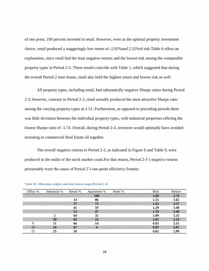
Table 10: Allocation weights and risk/return range (Period 2-4)
Office % Industrial % Retail % Apartment % Hotel % Risk Return
100 1.69 3.74
14 86 1.55 3.65
27 73 1.42 3.57
41 59 1.29 3.48
53 47 1.19 3.40
2 64 35 1.09 3.32
10 65 25 1.01 2.24
9 11 66 14 0.93 3.15
19 10 67 4 0.87 3.07
25 25 50 0.82 2.99

27
Period 2-4
As shown in Table 10, all five property types in Period 2-4, contrary to Period 2-3
produced positive returns. Risk-adverse investors could achieve low risk by investing 25% in
office and industrial properties each, and 50% in retail. That combination would allow investors
a 2.99% return for 0.82% of risk. Risk-taking investors, however, could invest solely in
apartments for a 3.74% return for 1.69% of risk. Most striking, as noted above, is that Period 2-4
actually produces superior returns relative to Period 1, as shown in Figure 3.
Also, contrary to the other Period 2 sub-periods, all five property types in Period 2-4
produced positive Sharpe coefficients. Retail offered the highestSharpe ratio of 3.27, while
hotels offered the lowest at 1.90. Those ratios aresignificantly higher than the proceeding Period
2 sub-periods, Period 2, and even Period 1. Property values fell so low during the 2008 crash that
as property values rise once again, returns do as well. Therefore, in terms of risk/return trade-
offs, Real Estate has since 2010 has become a more attractive investment than any time in the
past decade.
Summary
Between the four Period 2 sub-set periods, there is overwhelming evidence of economic
cycle volatility. In Period 2-1, from when the housing bubble burst to the sub-prime mortgage
market crash, hotel properties held the highest potential returns; yet, judging by risk/return trade-
off, office properties were most attractive; yet, after the sub-prime market collapse in 2007,
office properties held the highest Sharpe ratio and produced the highest returns. Conversely,
hotel properties at their peak contribution only made up 17% of the Period 2-2 optimal portfolio.
In Period 2-3 when the stock market collapsed, all property types produced negative returns, but

28
retail was the comparable best.Period 2-4 conversely offers diversification benefits, and shows
positive movements in regards to returns.

29
CONCLUSION
The results in this study show the impact that the bursting of the U.S. housing bubble had
on commercial real estate investing. Real estate from 2000 q1 to 2005 q2 (when the housing
bubble burst) produced superior return for risk relative to after the housing bubble 2005 q3 to
2012 q2, which only produced a one-point efficient frontier. In early 2007, the sub-prime
mortgage market collapsed and was the key event that led to rapidly declining property
values/returns and the market crash in the fall of 2008. Retail was the most attractive investment
in terms of return potentialbefore and after the housing bubble burst; however, retail also held the
lowest risk for highest return post housing bubble, making it an appealing sole optimization
choice. Examining sub-periods within the post bubble period shows that returns varied from
positive to substantially negative (during the 2008 crash time-frame). Thus, during different
cycles investors must adapt and strategize appropriately to capitalize on opportunities.As
investors further seek to eliminate unsystematic risk, diversification strategies and risk/return
analysis allow them to continue pursuing portfolio optimization.

30
REFERENCES
A-Petersen, G., & Singh, A. (2003). Performance of hotel investment in a multi-property
commercial real estate portfolio:Analysis of results from 1982 to 2001. Journal Of Retail
& Leisure Property, 3(2), 158-175.
Black, R. T. (2004). Real Estate in the Investment Portfolio.Real Estate Issues, 29(3), 1-6.
Cheng, P., Lin, Z., Liu, Y., & Zhang, Y. (2011). Has Real Estate Come of Age?.Journal Of Real
Estate Portfolio Management, 17(3), 243-254.
Fugazza, C., Guidolin, M., &Nicodanna, G. (2007). Investing for the long run in European
real estate. The Journal of Real Estate Finance and Economics, 34(1), 35–80.
Hui, E., & Yu, C. W. (2010).Enhanced portfolio optimisation model for real estate investment in
HK.Journal Of Property Research, 27(2), 147-180. doi:10.1080/09599916.2010.500873
Lai, R. N., & Van Order, R. A. (2010). Momentum and House Price Growth in the United States:
Anatomy of a Bubble. Real Estate Economics, 38(4), 753-773. doi:10.1111/j.1540-
6229.2010.00282.x
Lin, Z., &Vandell, K. D. (2007).Illiquidity and Pricing Biases in the Real Estate Market.Real
Estate Economics, 35(3), 291-330. doi:10.1111/j.1540-6229.2007.00191.x
Markowitz, H.M. (1952). Portfolio selection.Journal of Finance, 7, 77–91.
Mueller, G.R., Laposa, S.P. (1995), "Property-type diversification in real estate portfolios: size
and return perspective", The Journal of Real Estate Portfolio Management, Vol. 1 No.1,
pp.39-50.

31
Muller, A., Almy, R., &Engelschalk, M. (2010). Real Estate Bubbles and the Economic Crises:
The Role of Credit Standards and the Impact of Tax Policy. Journal Of Property Tax
Assessment & Administration, 7(1), 17-40.
Penny, P. E. (1982). Modern Investment Theory and Real Estate Analysis.Appraisal Journal,
50(1), 79.
Sivitanides, P. S. (1998). A Downside-Risk Approach to Real Estate Portfolio
Structuring.Journal Of Real Estate Portfolio Management, 4(2), 159.
Stephen, L., & Simon, S. (2005). Real estate portfolio construction and estimation risk. Journal
Of Property Investment & Finance, 23(3), 234-253.
Viezer, T. W. (2000). Evaluating `within real estate' diversification strategies.Journal Of Real
Estate Portfolio Management, 6(1), 75