Optimal Interest-Rate Rules in a Forward-Looking Model,

and In‡ation Stabilization versus Price-Level Stabilization¤

Marc P. Giannoniy

Federal Reserve Bank of New York

October 25, 2000

Abstract

This paper characterizes optimal monetary policy with commitment in a simpleforward-looking model. We propose a monetary policy rule that implements the op-timal plan. We then compare the performance of Taylor rules to price-level targetingrules (called Wicksellian rules). We argue that appropriate Wicksellian rules performgenerally better than optimal Taylor rules, because they result in a lower welfare loss,a lower variability of in‡ation and of nominal interest rates, by introducing desirablehistory dependence in monetary policy. Moreover, unlike optimal Taylor rules, whichmay result in indeterminacy of the equilibrium, Wicksellian rules do in general resultin a determinate equilibrium.

JEL Classi…cation: E30, E31, E52, E58.

Keywords: Optimal Monetary Policy, In‡ation Stabilization, Price-level Stabilization,Forward-looking.

¤This paper is part of my Ph.D. dissertation at Princeton University. I wish to thank Michael Woodford

for useful comments and suggestions. Any remaining errors are my own. The views are those of the author

and do not necessarily represent the views of the Federal Reserve Bank of New York or the Federal Reserve

System.yAddress: Federal Reserve Bank of New York, Domestic Research, 33 Liberty Street, New York, NY

10045. Email: marc.giannoni@ny.frb.org.

1 Introduction

Recent studies of monetary policy have emphasized the importance of history dependence

for the conduct of monetary policy. Woodford (1999c, 1999d, 2000b), has shown that when

agents are forward-looking, it is optimal for policymakers not only to respond to current

shocks and the current state of the economy, but that it is desirable to respond to lagged

variables as well. Committing to a monetary policy of this kind allows the central bank to

a¤ect the private sector’s expectations appropriately. This in turn improves the performance

of monetary policy because the evolution of the policymaker’s goal variables depends not

only upon its current actions, but also upon how the private sector foresees future monetary

policy.

In this paper, we investigate the implications of this history dependence for desirable

monetary policy rules (or instrument rules) in a simple forward-looking model. We …rst

propose an interest-rate feedback rule that implements the optimal plan. This policy rule

is characterized by a strong response of the current interest rate to lagged interest rates –

in fact a response to the lagged interest that is greater than one. Such super-inertial policy

rules have been advocated by Rotemberg and Woodford (1999), and Woodford (1999c),

for their ability to a¤ect expectations of the private sector appropriately. However Taylor

(1999b) has criticized super-inertial rules on robustness grounds.1 The concern for robust-

ness has led many authors to focus on very simple policy rules (see, e.g., Taylor, 1999a,

McCallum, 1988, 1999, and Levin et al., 1999). We therefore turn to very simple policy

rules that are not super-inertial. In particular, we compare the performance of standard

Taylor rules to interest-rate rules that involve responses to price-level variations (called

hereafter Wicksellian rules).

Previous studies have usually found that in‡ation targeting is more desirable than price-

level targeting. For example Lebow et al. (1992), and Haldane and Salmon (1995) show that

price-level targeting rules result in a higher short-run variability of in‡ation and output.2

The intuition for this result is simple: in the face of an unexpected temporary rise in

in‡ation, price-level targeting requires the policymaker to bring in‡ation below the target

in later periods, in order for the price level to return to its path. With nominal rigidities,

‡uctuations in in‡ation result in turn in ‡uctuations in output. In contrast, with in‡ation

targeting, the drift in the price level is accepted so that there is no need to generate a

de‡ation in subsequent periods. Thus price-level targeting is a “bad idea” according to1Taylor (1999b) shows that super-inertial rules perform poorly in non-rational expectations, backward-

looking, models. This should not be surprising since super-inertial rules rely precisely on the private sector’s

forward-looking behavior.2 In contrast, Fillion and Tetlow’s (1994) simulations indicate that price-level targeting results in lower

in‡ation variability but higher output variability than under in‡ation targeting. They however provide little

explanation for that result.

1

this conventional view because it would “add unnecessary short term ‡uctuations to the

economy” (Fischer, 1994, p. 282), while it would only provide a small gain in long-term

price predictability in the US (McCallum, 1999).

However, when agents are forward-looking and have rational expectations, this conven-

tional result is likely to be reversed. We argue that appropriate Wicksellian rules perform

generally better than optimal Taylor rules in the model considered. Wicksellian rules result

in a lower welfare loss, a lower variability of in‡ation and of nominal interest rates, by

introducing desirable history dependence in monetary policy. In the face of a temporary

increase in in‡ation, forward-looking agents expect relatively low in‡ation in subsequent

periods under price-level targeting, as the policymaker will have to bring in‡ation below

trend. This in turn dampens the initial increase in in‡ation, lowers the variability of in-

‡ation and rises welfare. Williams (1999) con…rms this result by simulating the large-scale

FRB/US model under alternative simple interest-rate rules. He reports that price-level

targeting rules result in lower in‡ation and output variability than in‡ation targeting rules

for a large set of parameter values, under rational expectations.3 Moreover, Wicksellian

rules have the desirable property of resulting in general in a determinate equilibrium, unlike

optimal Taylor rules, which may result in an indeterminate equilibrium.

We assume that the policymaker credibly commits to a policy rule for the entire future.

This approach, which has been advocated by McCallum (1988, 1999), Taylor (1993, 1999a),

and Woodford (1999c, 1999d) among others, allows the policymaker to achieve a better

performance of monetary policy by taking advantage not only of the gains from commit-

ment made popular by Kydland and Prescott (1977), but also of the e¤ect of a credible

commitment on the way the private sector forms expectations of future variables. The pol-

icy rules that we derive are time-consistent if policymakers take the “timeless perspective”

proposed by Woodford (1999d). Another branch of the recent literature assumes instead

that policymakers cannot credibly commit and that monetary policy is conducted under full

discretion. These studies generally compare the e¤ects of a regime in which the policymaker

is assigned a loss function that involves in‡ation variability (called in‡ation targeting), to

a regime in which the loss function involves price-level variability (price-level targeting).

Svensson (1999) and Dittmar et al. (1999) show that when the central bank acts under

discretion, and the perturbations to output are su¢ciently persistent, price-level targeting

results in lower in‡ation variability than in‡ation targeting. (However under commitment,

Svensson (1999) still obtains the conventional result that price-level targeting is responsible

for a higher variability of in‡ation.) While these authors use a Neoclassical Phillips curve,

Vestin (1999), and Dittmar and Gavin (2000) show that these results hold more generally3 In contrast, price-level targeting rules perform worse than in‡ation-targeting rules when the expectations

channel described above is shut o¤, i.e., when expectations are formed according to a forecasting model (VAR)

based on a regime of in‡ation targeting, and independent of the policy rule actually followed.

2

in a simple model with a “New Keynesian” supply equation — a simpli…ed version of the

model presented below. Speci…cally, they show that when the central bank acts under

discretion, price-level targeting results in a more favorable trade-o¤ between in‡ation and

output gap variability relative to in‡ation targeting, even when perturbations to output are

not persistent.4

The rest of the paper is organized as follows. Section 2 reviews the model. Section 3

describes the optimal response of endogenous variables to perturbations, under the optimal

plan and the plan in which history dependence is not allowed. Section 4 …rst determines

a policy rule that implements the optimal plan. It then compares optimal Taylor rules to

optimal Wicksellian rules. Section 5 concludes.

2 A Simple Optimizing Model

This section reviews a simple macroeconomic model that can be derived from …rst principles,

and that has been used in many recent studies of monetary policy (see Appendix A for

details).5 The behavior of the private sector is summarized by two structural equations,

an intertemporal IS equation and a “New Keynesian” aggregate supply equation. The

intertemporal IS equation, which relates spending decisions to the interest rate, is given by

Yt ¡ gt = Et (Yt+1 ¡ gt+1)¡ ¾¡1 (it ¡ Et¼t+1) ; (1)

where Yt denotes (detrended) real output, ¼t is the quarterly in‡ation rate, it is the nominal

interest rate (all three variables expressed in percent deviations from their values in a steady-

state with zero in‡ation and constant output growth), and gt is an exogenous variable

representing autonomous variation in spending such as government spending. This equation

can be obtained by performing a log-linear approximation to the representative household’s

Euler equation for optimal timing of consumption, and using the market clearing condition

on the goods market.6 The parameter ¾ > 0 represents the inverse of the intertemporal

elasticity of substitution. According to (1), consumption depends not only on the real

interest rate, but also on expected future consumption. This is because when they expect

to consume more in the future, households also want to consume more in the present, in4Kiley (1998) emphasizes that price-level targeting results in more expected variation in output relative

to in‡ation targeting, in a model with a “New Keynesian” supply equation.5The model is very similar to the one presented in Woodford (1999c). Variants of this model have

been used in a number of other recent studies of monetary policy such as Kerr and King (1996), Bernanke

and Woodford (1997), Goodfriend and King (1997), Rotemberg and Woodford (1997, 1999), Kiley (1998),

Clarida et al. (1999), and McCallum and Nelson (1999a, 1999b). Derivations of the structural equations

from …rst principles can be found in Woodford (1996, 1999b, 2000a).6The latter equation states that in equilibrium output is equal to consumption plus government expen-

ditures.

3

order to smooth their consumption. Note …nally that by iterating (1) forward, one obtains

Yt ¡ gt = ¡¾¡1Et1Xj=0

(it+j ¡ ¼t+1+j) :

This reveal that aggregate demand depends not only upon current short-term real interest

rates, but also upon expected long-term real rates, which are determined by expected future

short-term rates. It is important to note that current output is therefore a¤ected by the

private sector’s beliefs about future monetary policy.

It is assumed that prices are sticky, and that suppliers are in monopolistic competition.

It follows that the aggregate supply equation, which can be viewed as a log-linear approx-

imation to the …rst-order condition for the suppliers’ optimal price-setting decisions, is of

the form

¼t = · (Yt ¡ Y nt ) + ¯Et¼t+1; (2)

where Y nt represents the natural rate of output, i.e., the equilibrium rate of output under

perfectly ‡exible prices. The parameter · > 0 can be interpreted as a measure of the

speed of price adjustment, and ¯ 2 (0; 1) denotes the discount factor of the representativehousehold. The natural rate of output is a composite exogenous variable that depends in

general on a variety of perturbations such as productivity shocks, shifts in labor supply,

but also ‡uctuations in government expenditures and shifts in preferences (see Woodford,

1999b). Whenever the natural rate of output represents ‡uctuations in those variables,

then it corresponds also to the e¢cient rate of output, i.e., the rate of output that would

maximize the representative household’s welfare in the absence of distortions such as market

power.

Here, however, we allow the natural rate of output to di¤er from the e¢cient rate.

We assume exogenous time variation in the degree of ine¢ciency of the natural rate of

output. Such variation could be due for instance to exogenous variation in the degree of

market power of …rms, i.e., the desired markup. In this case, we show in Appendix A that

the percentage deviation of the e¢cient rate of output Y et from the natural rate Y nt (the

equilibrium level under ‡exible prices) is given by

Y et ¡ Y nt = (! + ¾)¡1 ¹t; (3)

where ¹t represents the percent deviation of desired markup from the steady-state, and

! > 0 is the elasticity of an individual …rm’s real marginal cost with respect to its own

supply, evaluated at the steady-state. As we will evaluate monetary policy in terms of

deviations of output from the e¢cient rate, it will be convenient to de…ne the “output gap”

as

xt ´ Yt ¡ Y et :

4

Using this, we can rewrite the structural equations (1) and (2) as

xt = Etxt+1 ¡ ¾¡1 (it ¡ Et¼t+1 ¡ ret ) (4)

¼t = ·xt + ¯Et¼t+1 + ut; (5)

where

ret ´ ¾Et£¡Y et+1 ¡ Y et

¢¡ (gt+1 ¡ gt)¤ut ´ · (Y et ¡ Y nt ) = · (! + ¾)¡1 ¹t:

In (4), ret denotes the “e¢cient” rate of interest, i.e., the equilibrium real interest rate that

would equate output to the e¢cient rate of output Y et . It is the real interest rate that would

prevail in equilibrium in the absence of distortions. Since the nominal interest rate enters

the structural equations only through the interest rate gap (it ¡ Et¼t+1 ¡ ret ) ; monetarypolicy is expansive or restrictive only insofar as the equilibrium real interest rate is below

or above the e¢cient rate. Note that if the equilibrium real interest rate was perfectly

tracking the path of the e¢cient rate, the output gap would be zero at all times, so that

equilibrium output would vary in tandem with the e¢cient rate of output, while in‡ation

would ‡uctuate only in response to the shocks ut:

We call the exogenous disturbance ut in (5) an “ine¢cient supply shock” since it repre-

sents a perturbation to the natural rate of output that is not e¢cient. Time variation in the

degree of e¢ciency of the natural rate of output is understood as representing exogenous

time variation in the desired markup on the goods market, but it could alternatively be

interpreted as time variation in distortionary tax rates or exogenous variation in the degree

of market power of workers on the labor market. We prefer to call ut an “ine¢cient supply

shock” rather then a “cost-push shock” as is often done in the literature (see, e.g., Clarida

et al., 1999), because perturbations that a¤ect in‡ation by changing costs of production

do not necessarily a¤ect the degree of ine¢ciency of the natural rate of output. Indeed,

cost shocks (due, e.g., to perturbations to energy prices) may well shift the e¢cient rate of

output as well as the natural rate of output. Such shocks are therefore represented in our

model by changes in the output gap xt; rather than disturbances to ut:

As we will also be interested in describing the evolution of the log of the price level pt;

we note that by de…nition of in‡ation, we have

pt = ¼t + pt¡1: (6)

We now turn to the goal of monetary policy. We assume that the policymaker seeks to

minimize the following loss criterion

L0 = E0

((1¡ ¯)

1Xt=0

¯th¼2t + ¸x (xt ¡ x¤)2 + ¸i (it ¡ i¤)2

i); (7)

5

where ¸x; ¸i > 0 are weights placed on the stabilization of the output gap and the nominal

interest rate, ¯ 2 (0; 1) is the discount factor mentioned above, and where x¤ ¸ 0 and

i¤ represent some optimal levels of the output gap and the nominal interest rate. Thisloss criterion can be viewed as a second-order Taylor approximation to the lifetime utility

function of the representative household in the underlying model (see Woodford 1999b).

The presence of the interest rate variability re‡ects both welfare costs of transactions …rst

mentioned by Friedman (1969), and the fact that the nominal interest rate has a lower bound

at zero.7 The approximation of the utility function allows us furthermore to determine the

relative weights ¸x; ¸i; and the parameters x¤; i¤ in terms of the parameters of the underlyingmodel.8

We will assume that the policymaker chooses monetary policy in order to minimize

the unconditional expectation E [L0] where the expectation is taken with respect to the

stationary distribution of the shocks. It follows that optimal monetary policy is independent

of the initial state. As Woodford (1999d) explains, such a policy is furthermore time-

consistent if the central bank adopts a “timeless perspective”, i.e., if it chooses “the pattern

of behavior to which it would have wished to commit itself to at a date far in the past,

contingent upon the random events that have occurred in the meantime ” (Woodford,

1999d).

The ine¢cient supply shock is responsible for a trade-o¤ between the stabilization of

in‡ation on one hand, and the output gap on the other hand. Indeed, in the face of an

increase in ut; the policymaker could completely stabilize the output gap by letting in‡ation

move appropriately, or he could stabilize in‡ation, by letting the output gap decrease by

the right amount, but he could not keep both in‡ation and the output gap constant. By

how much he will let in‡ation and the output gap vary depends ultimately on the weight

¸x: In the absence of ine¢cient supply shocks, however, the policymaker could in principle

completely stabilize both in‡ation and the output gap by letting the interest rate track

the path of the e¢cient rate of interest, ret (which incidentally is equal to the natural rate

of interest in the absence of ine¢cient supply shocks, as Y et = Y nt ). But when ¸i > 0 in

(7), welfare costs associated to ‡uctuations in the nominal interest rate introduce a tension

between stabilization of in‡ation and the output gap on one hand, and stabilization of the

nominal interest rate on the other hand.7According to Friedman (1969), the welfare costs of transactions are eliminated only if nominal interest

rates are zero in every period. Assuming that the deadweight loss is a convex function of the distortion, it

is not only desirable to reduce the level , but also the variability of nominal interest rates.8Woodford (1999b) abstracts from ine¢cient supply shocks. His derivation of the loss criterion from …rst

principles is essentially una¤ected by the introduction of ine¢cient supply shocks. One di¤erence, however,

is that the loss function involves the deviation of output from its e¢cient rate, and not from its natural rate.

Moreover, when the desired markup, ¹t; is exogenously time varying, the parameters of the loss function are

function of the steady-state markup ¹¹ instead of some constant value ¹:

6

In the rest of the paper, we will characterize optimal monetary policy for arbitrary posi-

tive values of the parameters. At times however we will focus on a particular parametrization

of the model, using the parameter values estimated by Rotemberg and Woodford (1997) for

the U.S. economy, and summarized in Table 1. While the econometric model of Rotemberg

and Woodford (1997) is more sophisticated than the present model, their structural equa-

tions correspond to (1) and (2) when conditioned upon information available two quarters

earlier in their model. The weights ¸x and ¸i are calibrated as in Woodford (1999c), using

the calibrated structural parameters and the underlying microeconomic model. Rotemberg

and Woodford (1997) provide estimated time-series for the disturbances Y nt and gt: They

do however not split the series for the natural rate of output in an e¢cient component Y et ;

and an ine¢cient component. For simplicity, we calibrate the variance of ret by assuming

that all shifts in the aggregate supply equation are e¢cient shifts, so that the variance

of the e¢cient rate of interest is the same as the variance of the natural rate of interest

reported in Woodford (1999c). Inversely, we calibrate var (ut) by assuming that all shifts in

the aggregate supply equation are due to ine¢cient shocks. By de…nition of ut; this upper

bound for var (ut) is given by var (ut) = ·2 var (Y nt ) :

3 Optimal Responses to Perturbations

In this section, we characterize the optimal response of endogenous variables to the two

kinds of perturbations relevant in the model presented above: disturbances to the e¢cient

rate of interest, and ine¢cient supply shocks. We generalize the results of Woodford (1999c)

by introducing ine¢cient supply shocks. Clarida et al. (1999) and Woodford (1999d) have

also characterized the optimal plan in the presence of ine¢cient supply shocks, but they

assume that ¸i = 0 in the loss function, while we let ¸i > 0:

3.1 Optimal Plan

The optimal plan is characterized by the stochastic processes of endogenous variables

f¼t; xt; itg that minimize the unconditional expectation of the loss criterion (7) subjectto the constraints (4) and (5) at all dates. It speci…es the entire future state-contingent

evolution of endogenous variables as of date zero. As will become clearer in the next sec-

tion, this corresponds to a plan to which the policymaker is assumed to commit for the

entire future. Following Currie and Levine (1993) and Woodford (1999c), we write the

policymaker’s Lagrangian as

L = E

(E0

1Xt=0

¯tµ1

2

h¼2t + ¸x (xt ¡ x¤)2 + ¸i (it ¡ i¤)2

i+Á1t

£xt ¡ xt+1 + ¾¡1 (it ¡ ¼t+1 ¡ ret )

¤+ Á2t [¼t ¡ ·xt ¡ ¯¼t+1 ¡ ut]

¢ª: (8)

7

The …rst-order necessary conditions with respect to ¼t; xt; and it are

¼t ¡ (¯¾)¡1 Á1t¡1 + Á2t ¡ Á2t¡1 = 0 (9)

¸x (xt ¡ x¤) + Á1t ¡ ¯¡1Á1t¡1 ¡ ·Á2t = 0 (10)

¸i (it ¡ i¤) + ¾¡1Á1t = 0 (11)

at each date t ¸ 0; and for each possible state. In addition, we have the initial conditions

Á1;¡1 = Á2;¡1 = 0 (12)

indicating that the policymaker has no previous commitment at time 0.

The optimal plan is a bounded solution f¼t; xt; it; Á1t; Á2tg1t=0 to the system of equations(4), (5), (9) – (11) at each date t ¸ 0; and for each possible state, together with the initialconditions (12). We …rst determine the steady-state values of the endogenous variables of

interest that satisfy the previous equations at all dates in the absence of perturbations.

They are given by

iop = ¼op =¸ii

¤

¸i + ¯; xop =

1¡ ¯·

¸ii¤

¸i + ¯: (13)

Note that the optimal steady-state in‡ation is independent of x¤: It follows that when theoptimal nominal interest rate i¤ = 0; steady-state in‡ation is zero in the optimal plan,

whether the steady-state output level is ine¢cient (x¤ > 0) or not. However, in general

when ¼op 6= 0; the log price level follows a deterministic trend

popt = ¼op + popt¡1:

To characterize the optimal responses to perturbations, we de…ne ¼t ´ ¼t ¡ ¼op; xt ´xt ¡ xop; {t ´ it ¡ iop; and pt ´ pt ¡ popt ; and rewrite the equations above in terms ofdeviations from the steady-state values. We note that the same equations (4), (5), (9) –

(11), and (6) hold now in terms of the hatted variables, but without the constant terms.

Using (11) to substitute for the interest rate, we can rewrite the dynamic system (4), (5),

(9), and (10) in matrix form as

Et

"zt+1

Át

#=M

"zt

Át¡1

#+met; (14)

where zt ´ [¼t; xt]0 ; Át ´hÁ1t; Á2t

i0; et ´ [ret ; ut]0 ; andM andm are matrices of coe¢cients.

Following Blanchard and Kahn (1980), this dynamic system has a unique bounded solution

(given a bounded process fetg) if and only if the matrix M has exactly two eigenvalues

outside the unit circle. Investigation of the matrix M reveals that if a bounded solution

8

exists, it is unique.9 In this case the solution for the endogenous variables can be expressed

as

qt = DÁt¡1 +1Xj=0

djEtet+j; (15)

where qt ´ [¼t; xt; {t; pt]0 ; and the Lagrange multipliers follow the law of motion

Át = NÁt¡1 +1Xj=0

njEtet+j (16)

for some matrices D; N; dj; nj that depend upon the parameters of the model. Woodford

(1999c) has emphasized that in the optimal plan, the endogenous variables should depend

not only upon expected future values of the disturbances, but also upon the predetermined

variables Át¡1. This dependence indicates that optimal monetary policy should involveinertia in the interest rate, regardless of the possible inertia in the exogenous shocks.

3.2 Optimal Non-Inertial Plan

To evaluate more directly the importance of the history dependence in the optimal plan,

we compare the latter to a plan in which policy is prevented from responding to lagged

variables. Following Woodford (1999c), we call this plan the optimal non-inertial plan.

As we will see in the next section, this plan is furthermore interesting because it can be

implemented by a simple Taylor rule.

For simplicity, we assume that the exogenous shocks follow univariate stationary AR(1)

processes

ret = ½rret¡1 + "rt (17)

ut = ½uut¡1 + "ut; (18)

where the disturbances "rt; "ut are unforecastable one period in advance, and E("rt) =

E ("ut) = 0; E("rt"ut) = 0; ­r ´ E¡"2rt¢> 0; ­u ´ E

¡"2ut¢> 0; and 0 · ½r; ½u < 1: In

this case, the equilibrium evolutions of the endogenous variables in the optimal non-inertial

plan can be described by

¼t = ¼ni + ¼rr

et + ¼uut; xt = x

ni + xrret + xuut; it = i

ni + irret + iuut; (19)

where ¼ni; xni; ini are the steady-state values of the respective variables in this optimal

equilibrium, and ¼r; ¼u; and so on, are the optimal equilibrium response coe¢cients to ‡uc-

tuations in ret and ut: For the solution (19) to correspond to an equilibrium, the coe¢cients9The matrix M has two eigenvalues with modulus greater than ¯¡1=2 and two with modulus smaller than

this.

9

¼ni; ¼r; ¼u; and so on, need to satisfy the structural equations (4) and (5) at each date, and

for every possible realization of the shocks. These coe¢cients need therefore to satisfy the

following feasibility restrictions, obtained by substituting (19) into the structural equations

(4) and (5):

(1¡ ¯)¼ni ¡ ·xni = 0 (20)

¼ni ¡ ini = 0 (21)

(1¡ ½r)xr + ¾¡1 (ir ¡ ½r¼r ¡ 1) = 0 (22)

(1¡ ¯½r)¼r ¡ ·xr = 0 (23)

(1¡ ½u)xu + ¾¡1 (iu ¡ ½u¼u) = 0 (24)

(1¡ ¯½u)¼u ¡ ·xu ¡ 1 = 0: (25)

Similarly, substituting (19) into (7), and using E(retut) = 0; we can rewrite the loss function

as

E [L0] =h¡¼ni¢2+ ¸x

¡xni ¡ x¤¢2 + ¸i ¡ini ¡ i¤¢2i+ ¡¼2r + ¸xx2r + ¸ii2r¢ var (ret )

+¡¼2u + ¸xx

2u + ¸ii

2u

¢var (ut) :

To determine the optimal non-inertial plan, we choose the equilibrium coe¢cients that

minimize the loss E [L0] subject to the restrictions (20) – (25). The steady-state of the

optimal non-inertial equilibrium is given by

ini = ¼ni =(1¡ ¯)·¡1¸xx¤ + ¸ii¤1 + (1¡ ¯)2 ·¡2¸x + ¸i

; xni =1¡ ¯·

(1¡ ¯)·¡1¸xx¤ + ¸ii¤1 + (1¡ ¯)2 ·¡2¸x + ¸i

; (26)

and the optimal response coe¢cients to ‡uctuations in ret and ut in the optimal non-inertial

equilibrium are given by

¼r =¸i (¾°r ¡ ½r·)·

hr; ¼u =

¸i¾ (¾°u ¡ ½u·) (1¡ ½u) + ¸x (1¡ ¯½u)hu

(27)

xr =¸i (¾°r ¡ ½r·) (1¡ ¯½r)

hr; xu = ¡·¡ ½u¸i (¾°u ¡ ½u·)

hu(28)

ir =¸x (1¡ ¯½r)2 + ·2

hr; iu =

¾· (1¡ ½u) + ¸x (1¡ ¯½u) ½uhu

; (29)

where

°j ´ ¡1¡ ½j

¢ ¡1¡ ¯½j

¢> 0

hj ´ ¸i¡¾°j ¡ ½j·

¢2+ ¸x

¡1¡ ¯½j

¢2+ ·2 > 0;

and where j 2 fr; ug :

10

It is clear from (29) that both ir and iu are positive for any positive weights ¸i; ¸x: Thus

the optimal non-inertial plan involves an adjustment of the nominal interest rate in the

direction of the perturbations. Equations (27) and (28) reveal that the response coe¢cients

¼r; xr are positive if and only if

¾

·>

½r(1¡ ¯½r) (1¡ ½r)

; (30)

that is, whenever the ‡uctuations in the e¢cient rate are not too persistent (relative to the

ratio ¾· ). Thus when (30) holds, a positive shock to the e¢cient rate stimulates aggregate

demand, so that both the output gap and in‡ation increase. In the special case in which

the interest rate does not enter the loss function (¸i = 0), or when the persistence of the

perturbations is such that ¾ (1¡ ¯½r) (1¡ ½r) = ½r·; we obtain ¼r = xr = 0 and ir = 1: Asa result, in the absence of ine¢cient supply shocks, the central bank optimally moves the

interest rate by the same amount as the e¢cient rate in order to stabilize the output gap

and in‡ation completely.

When the disturbances to the e¢cient rate are su¢ciently persistent (½r large enough

but still smaller than 1) for the inequality (30) to be reversed, in‡ation and the output gap

decrease in the face of an unexpected positive shock to the e¢cient rate in the optimal non-

inertial plan. Even if the nominal interest rate increases less than the natural rate, optimal

monetary policy is restrictive in this case, because the real interest rate (it ¡Et¼t+1) ishigher than the e¢cient rate of interest ret .

3.3 Description of Impulse Responses and Moments

We now illustrate the properties of the optimal plan and the optimal non-inertial plan by

looking at the response of endogenous variables to an unexpected disturbance to the e¢cient

rate of interest or to an unexpected ine¢cient supply shock, when we adopt the calibration

summarized in Table 1.

Shock to ret : Figure 1a plots the optimal response of the interest rate, in‡ation, the

output gap, and the price level to an unexpected temporary increase in the e¢cient rate

of interest (or equivalently the natural rate of interest, as it is assumed that there is no

ine¢cient supply shock) when ½r = 0.10 Such an increase in ret may re‡ect an exogenous

increase in demand (represented by gt) and/or an adverse supply shock represented by a

decrease in Y et . One period after the shock, the e¢cient rate of interest is expected to be

back at its steady-state value; its expected path is indicated by a dotted line in the upper

panel.10The responses of all variables are reported in annual terms. Therefore, the responses of {t and ¼t are

multiplied by 4.

11

As discussed above, the nominal interest rate increases by less than the natural rate of

interest in the optimal non-inertial plan (dashed lines), in order to dampen the variability

of the nominal interest rate (which enters the loss function). Monetary policy is therefore

relatively expansionary so that in‡ation and the output gap increase at the time of the

shock. In later periods however, these variables return to their initial steady-state in the

optimal non-inertial plan, as the perturbation vanishes.

In contrast, in the optimal plan illustrated by solid lines, the short-term interest rate is

more inertial than the e¢cient rate. Inertia in monetary policy is especially desirable here

because it induces the private sector to expect future restrictive monetary policy, hence

future negative output gaps which in turn have a disin‡ationary e¤ect already when the

shock hits the economy. Thus the expectation of an inertial policy response allows the

policymaker to o¤set the in‡ationary impact of the shock by raising the short-term interest

rate by less than in the optimal non-inertial plan. Note that at the time of the shock, the

price level is expected to decline as a result of future restrictive monetary policy. Although

the perturbation is purely transitory, the price level is expected to end up at a slightly lower

level in the future, in the optimal plan.

Figures 1b and 1c illustrate the impulse responses of the same variables when the shock

to the e¢cient rate of interest is more persistent. The path that the e¢cient rate is expected

to follow is described by an AR(1) process with a coe¢cient of autocorrelation of 0:35; and

0:9. In the optimal non-inertial plan, the nominal interest rate remains above steady-state

as long as the shock is expected to a¤ect the economy, but as in the purely transitory case,

the interest rate increases by less than the e¢cient rate of interest. Note that in‡ation and

the output gap decline below steady-state on impact when ½r = 0:9; as the equilibrium

real interest rate is higher than the e¢cient real interest rate in this case (condition (30) is

violated). In the optimal plan, the nominal interest rate increases initially by less than in

the optimal non-inertial plan, but is expected to be higher than the e¢cient rate in later

periods. Again, as people expect monetary policy to remain tight in the future, the output

gap is expected to be negative in the future. This removes pressure on in‡ation already

at the time of the shock, and the price level is expected to end up at a lower level in the

future.

Shock to ut: We now turn to the e¤ects of an unexpected ine¢cient supply shock. Figure

2a illustrates the optimal response of endogenous variables to a purely transitory rise in ut,

that is when the latter follows the process (18) with ½u = 0: In the optimal non-inertial plan

(dashed lines), the policymaker is expected to stabilize the variables at their steady state

in future periods, after the shock has disappeared. At the time of the (adverse) shock, it is

optimal to raise the nominal interest rate in order to reduce output (gap), and therefore to

remove some in‡ationary pressure. In the optimal plan (solid lines), however, it is optimal

12

to maintain the output gap below steady state for several periods, even if the disturbance

is purely transitory. This generates the expectation of a slight de‡ation in later periods

and thus helps dampening the initial increase in in‡ation. The last panel con…rms that the

price level initially rises with the adverse shock but then declines back to almost return to

its initial steady-state level. In fact the new steady-state price level is slightly below the

initial one. The optimal interest rate that is consistent with the paths for in‡ation and the

output gap hardly deviates from the steady-state. It is however optimal to slightly raise

the interest rate, and to maintain it above steady-state for several periods, to achieve the

desired de‡ation in later periods.

Figures 2b and 2c illustrate the optimal responses when ut follows the same process

but with coe¢cient of autocorrelation of 0:35 and 0:9: They reveal that the mechanisms

described above still work, even though the response of each variable is more sluggish.

Moments. The previous …gures reveal that, in the optimal non-inertial plan, the e¤ects

of perturbations on in‡ation, output gap and the interest rate last only as long as the shocks

last. In contrast, in the optimal plan, the e¤ects of disturbances last longer. Yet the loss

is lower in the optimal plan, as the variability of in‡ation and the interest rate is reduced

by allowing the policy to respond to past variables. This can be seen from Table 2, which

reports the policymaker’s loss, E [L0] ; in addition to the following measure of variability

V [z] ´ E(E0

"(1¡ ¯)

1Xt=0

¯tz2t

#)for the four endogenous variables, ¼; x; i; and p; where the unconditional expectation is

taken over all possible histories of the disturbances. Note that the loss E [L0] is a weighted

sum of V [¼] ; V [x] ; and V [i] with weights being the ones of the loss (7). The table reports

the statistics in the case in which x¤ = i¤ = 0; so that the steady state is the same for eachplan (and is zero for each variable). The statistics measure therefore the variability of each

variable around its steady state, and the column labeled with E [L0] indicates the loss due

to temporary disturbances in excess of the steady-state loss.11

A comparison of the statistics in Table 2 for the optimal plan and the optimal non-

inertial plan reveals that there are substantial gains from history dependence in monetary

policy. For instance, when ½r = ½u = 0:35; as in the baseline calibration, the loss is 1.28 in

the optimal plan, while it is 2.63 in the optimal non-inertial plan. The welfare gains due to

inertial monetary policy are primarily related to a lower variability of in‡ation and of the

nominal interest rate.11All statistics in Table 2 are reported in annual terms. The statistics V [¼] ; V [i] ; and E [L0] are therefore

multiplied by 16. Furthermore, the weight ¸x reported in Table 1 is also multiplied by 16 in order to

represent the weight attributed to the output gap variability (in annual terms) relative to the variability of

annualized in‡ation and of the annualized interest rate.

13

4 Optimal Policy Rules

So far, we have characterized how the endogenous variables should respond to perturbations

in order to minimize the welfare loss. We haven’t said anything about how monetary policy

should be conducted, especially if the shocks are not observed by policymakers. To this

issue, we now turn. Following recent studies of monetary policy (see, e.g., Taylor, 1999a),

we characterize monetary policy in terms of interest-rate feedback rules. Speci…cally, we

assume that the policymaker commits credibly at the beginning of period 0 to a policy

rule that determines the nominal interest rate as a function of present and possibly past

observable variables, at each date t ¸ 0.First, we propose a simple monetary policy rule that implements the optimal plan,

even when the perturbation are not observed. We then determine optimal policy rules in

restricted families: we compute optimal Taylor rules and then optimal Wicksellian rules,

i.e., interest-rate rules that respond to deviations of the price level from some deterministic

trend. Finally, we compare the performance of Taylor rules and Wicksellian rules.

4.1 Commitment to an Optimal Rule

We now turn to the characterization of an optimal monetary policy rule. As will become

clear below, there exists a unique policy rule of the form

it = ü¼t + Ãx (xt ¡ xt¡1) + Ãi1it¡1 + Ãi2it¡2 + Ã0 (31)

at all dates t ¸ 0; that is fully optimal, i.e., that implements the optimal plan described inthe previous section.12 To obtain the optimal rule, we solve (11) for Á1t and (10) for Á2t;

and use the resulting expressions to substitute for the Lagrange multipliers in (9). This

yields

it =·

¸i¾¼t +

¸x¸i¾

(xt ¡ xt¡1) +µ1 +

·

¯¾+ ¯¡1

¶it¡1 ¡ ¯¡1it¡2 ¡ ·i

¤

¯¾: (32)

This is an equilibrium condition that relates the endogenous variables in the optimal plan. It

can alternatively be viewed as an optimal rule, provided that it results in a unique bounded

equilibrium. Using (13), we can rewrite the same policy rule in terms of hatted variables,

by dropping the constant ·i¤¯¾ : The dynamic system obtained by combining (4), (5), and

12As we evaluate monetary policy regardless of speci…c initial conditions, the policy rule is assumed to be

independent of the values the endogenous variables might have taken before it was implemented. Speci…cally,

we assume that the policymaker considers the initial values as satisfying i¡2 = i¡1 = x¡1 = 0; whether they

actually do or not. Equivalently, we could assume that the policy rule satis…es i0 = ü¼0+Ãxx0; i1 = ü¼1+ Ãx (x1 ¡ x0) + Ãi1i0; and (31) at all dates t ¸ 2:

14

(32), has the property of system (14) that, if any bounded solution exists, it is unique.13

Moreover as we show in Appendix B.1, (32) is the unique optimal policy rule in the family

(31), at least in the baseline parametrization.

Notice that this rule makes no reference to either the e¢cient rate of interest ret or

the ine¢cient supply shock ut. It achieves the minimal loss regardless of the stochastic

process that describes the evolution of the exogenous disturbances, provided that the latter

are stationary (bounded). The policymaker achieves the optimal equilibrium by setting the

interest rate according to (32) even if the natural rate and the ine¢cient supply shock depend

upon a large state vector representing all sorts of perturbations such as productivity shocks,

autonomous changes in aggregate demand, labor supply shocks, etc. Another advantage of

this family of policy rules is that it includes recent descriptions of actual monetary policy

such as the one proposed by Judd and Rudebusch (1998). If we would allow for a broader

family of policy rules than (31), then other interest-rate feedback rules may implement the

same optimal plan. In the case in which there are no ine¢cient supply shocks, Woodford

(1999c), for example, proposes a rule in which the interest rate depends upon current and

lagged values of the in‡ation rate as well as lagged interest rates. While his rule makes no

reference to the output gap, it is dependent upon the driving process of the e¢cient rate of

interest.

Equation (32) indicates that to implement the optimal plan, the central bank should

relate the interest rate positively to ‡uctuations in current in‡ation, in changes of the

output gap, and in lagged interest rates. While it is doubtful that the policymaker knows

the current level of the output gap with great accuracy, the change in the output gap may

be known with greater precision. For example, Orphanides (1998) shows that subsequent

revisions of U.S. output gap estimates have been quite large (sometimes as large as 5.6

percentage points), while revisions of estimates of the quarterly change in the output gap

have been much smaller.

Note …nally that the interest rate should not only be inertial in the sense of being

positively related to past values of the interest rate, it should be super-inertial, as the

lagged polynomial for the interest rate in (32)

1¡µ1 +

·

¯¾+ ¯¡1

¶L + ¯¡1L2 = (1¡ z1L) (1¡ z2L)

involves a root z1 > 1 while the other root z2 2 (0; 1) : A reaction greater than one of theinterest rate to its lagged value has initially been found by Rotemberg and Woodford (1999)

to be a desirable feature of a good policy rule in their econometric model with optimizing13The eigenvalues of this system are the same as the eigenvalues of M in (14) plus one eigenvalue equal

to zero. As there is one predetermined variable more than in (14), this system yields a unique bounded

equilibrium, if it exists.

15

agents. As explained further in Woodford (1999c), it is precisely such a super-inertial policy

rule that the policymaker should follow to bring about the optimal responses to shocks when

economic agents are forward-looking. Because of a root larger than one, the optimal policy

requires an explosively growing response of the interest rate to deviations of in‡ation and

the output gap from the target (which is 0).

This is illustrated in Figure 3 which displays the response of the interest rate to a

sustained 1 percent deviation in in‡ation (upper panel) or the output gap (lower panel)

from target. In each panel, the solid line represents the optimal response in the baseline

case. The corresponding coe¢cients of the optimal policy rule are reported in the upper

right panel of Table 2.14 For comparison, the last panel of Table 2 reports the coe¢cients

derived from Judd and Rudebusch’s (1998) estimation of actual Fed reaction functions

between 1987:3 and 1997:4, along with the statistics that such a policy would imply if

the model provided a correct description of the actual economy.15 As shown on Table 2,

the estimated historical rule in the baseline case involves only slightly smaller responses to

‡uctuations in in‡ation and the output gap than the optimal rule. However the estimated

response to lagged values of the interest rate is sensibly smaller that the optimal one. As a

result, the estimated historical rule involves a non-explosive response of the interest rate to

a sustained deviation in in‡ation or the output gap, represented by the dashed-dotted lines

in Figure 3.

While optimal policy would involve an explosive behavior of the interest rate in the face

of a sustained deviation of in‡ation or the output gap, such a policy is perfectly consistent

with a stationary rational expectations equilibrium, and a low variability of the interest rate

in equilibrium. (In Table 2, V [i] is always smaller when the interest rate is set according

to the optimal ‡exible rule, than when it is set according to the estimated historical rule or

the optimal Taylor rule to be discussed below.) In fact, the interest rate does not explode in

equilibrium because (as appears clearly in Figures 1 and 2) the current and expected future

optimal levels of the interest rate counteract the e¤ects of an initial deviation in in‡ation

and the output gap by generating subsequent deviations with the opposite sign of these

variables.

While the policy rule (32) allows the policymaker to achieve the lowest possible loss,

recent research has given considerable attention to even simpler policy rules (see, e.g., con-

tributions collected in Taylor, 1999a). In addition, super-inertial rules have been criticized

on robustness grounds. In fact, the ability of super-inertial rules to perform well depends

critically on the assumption that each agent knows the model of the economy, and that14The coe¢cients Ãx reported here are multiplied by 4, so that the response coe¢cients to output gap,

and to annualized in‡ation are expressed in the same units. (See footnote 11.)15The estimated historical policy rule refers to regression A for the Greenspan period in Judd and Rude-

busch (1998).

16

the private sector understands the way monetary policy will be conducted in the future.

As Taylor (1999b) reports, these rules perform poorly in models which involve no rational

expectations and no forward-looking behavior.16 We therefore turn to very simple policy

rules that are not super-inertial.

4.2 Commitment to a Standard Taylor Rule

We proceed with the standard “Taylor rule” made popular by Taylor (1993), and satisfying

it = ü¼t + Ãxxt + Ã0; (33)

at all dates t ¸ 0; where ü; Ãx; and Ã0 are policy coe¢cients. For simplicity, we assumeagain that the law of motion of the shocks is given by (17) and (18). Using (33) to substitute

for the interest rate in the structural equations (4) and (5), we can rewrite the resulting

di¤erence equations as follows

Etzt+1 = Azt + aet; (34)

where zt ´ [¼t; xt; 1]0 ; and et ´ [ret ; ut]0 and A and a are matrices of coe¢cients. Since both¼t and xt are non-predetermined endogenous variables at date t; and fetg is assumed to bebounded, the dynamic system (34) admits a unique bounded solution if and only if A has

exactly two eigenvalues outside the unit circle.17 If we restrict our attention to the case in

which ü; Ãx ¸ 0; then it is shown in Appendix B.2 that the policy rule (33) results in adeterminate equilibrium if and only if

ü +1¡ ¯·

Ãx > 1: (35)

In this case, we can solve (34) for zt: Using (33) to determine also the equilibrium evolution

of the interest rate, one realizes that the equilibrium in‡ation, output gap, and nominal

interest rate are in fact given by expressions of the form (19). It follows that the optimal

Taylor rule is the rule that implements the optimal equilibrium of the form (19), i.e., the

optimal non-inertial plan characterized by (26) – (29).16However, Levin et al. (1999) show that rules that have a coe¢cient of one on the lagged interest rate

perform well across models. Moreover, in Giannoni (1999), it is shown that a variant of the super-inertial

rule discussed above is robust to uncertainty about the parameters of the model and the stochastic process

of the shocks.17Note that here, we implicitly assume that …scal policy is “Ricardian”, using the terminology proposed

by Woodford (1995). Papers that study determinacy of the rational expectations equilibrium in monetary

models with “non-Ricardian” …scal policy include Leeper (1991), Sims (1994), Woodford (1994, 1995, 1996,

1998b), Loyo (1999), and Schmitt-Grohé and Uribe (2000).

17

The optimal Taylor rule can be obtained by substituting the solution (19) into (33).

This yields three restrictions upon the coe¢cients of the policy rule

ir = ü¼r + Ãxxr (36)

iu = ü¼u + Ãxxu (37)

ini = ü¼ni + Ãxx

ni + Ã0: (38)

Notice that if all supply shocks are e¢cient, so that all disturbances can be represented by

the e¢cient (or natural) rate of interest, the constraint (37) is not relevant. As (36) and (38)

form a system of two equations in three unknown coe¢cients ü; Ãx; and Ã0, there exist

many Taylor rules that implement the optimal non-inertial plan in this case (see Giannoni,

1999, for more details). However in general, when we allow for both perturbations to the

e¢cient rate of interest and ine¢cient supply shock, there is a unique optimal Taylor rule.

Solving the …rst two restrictions for the policy coe¢cients ü; Ãx; yields

ü =xuir ¡ iuxrxu¼r ¡ ¼uxr

Ãx =¼riu ¡ ir¼uxu¼r ¡ ¼uxr ;

provided that xu¼r ¡ ¼uxr 6= 0: Finally, using the expressions (27) – (29) to substitute forthe coe¢cients ¼r; xr; :::; characterizing the optimal non-inertial equilibrium, we obtain the

coe¢cients of the optimal Taylor rule

ü =(·¡ ½u¸i (¾°u ¡ ½u·))

¡»r (1¡ ¯½r) + ·2

¢+ (¾· (1¡ ½u) + ½u»u)¸i (¾°r ¡ ½r·) (1¡ ¯½r)

¸i (¾°r ¡ ½r·) ((·¡ ½u¸i (¾°u ¡ ½u·))·+ (¸i¾ (¾°u ¡ ½u·) (1¡ ½u) + »u) (1¡ ¯½r))(39)

Ãx =(¸i¾ (¾°u ¡ ½u·) (1¡ ½u) + »u)

¡»r (1¡ ¯½r) + ·2

¢¡ ¸i (¾°r ¡ ½r·)· (¾· (1¡ ½u) + ½u»u)¸i (¾°r ¡ ½r·) ((·¡ ½u¸i (¾°u ¡ ½u·))·+ (¸i¾ (¾°u ¡ ½u·) (1¡ ½u) + »u) (1¡ ¯½r))

(40)

where »j ´ ¸x¡1¡ ¯½j

¢> 0; and j 2 fr; ug : Note that these expressions are well de…ned

provided that ¸i > 0 and ¾°r ¡ ½r· 6= 0: (The limiting case in which ¸i = 0 is discussed

below). Finally, the constant Ã0 is obtained by solving (38), using the optimal values for

ü and Ãx; and the steady-state expressions (26).

While the optimal Taylor rule depends in a complicated way on all parameters of the

model and the degree of persistence of the perturbations, it is interesting to note that it is

completely independent of the variability of the disturbances. Table 2 reports the optimal

coe¢cients (39) and (40) for di¤erent degrees of persistence of the perturbations, using

the calibration summarized in Table 1. These coe¢cients are displayed in Figure 4. The

white region of Figure 4 indicates the set of policy rules that result in a unique bounded

18

equilibrium. In contrast, the gray region indicates combinations (ü; Ãx) that result in

indeterminacy of the equilibrium.18

Figure 4 reveals for example that when both shocks are purely transitory (½r = ½u =

0), the “optimal” Taylor rule lies in the region of indeterminacy. In fact, the “optimal”

coe¢cients ü; Ãx, while positive, are not large enough to satisfy (35). This means that

for any bounded solution fztg to the di¤erence equation (34), there exists another boundedsolution of the form

z0t = zt + v»t

where v is an appropriately chosen (nonzero) vector, and the stochastic process f»tg mayinvolve arbitrarily large ‡uctuations, which may or may not be correlated with the funda-

mental disturbances ret and ut: It follows that the dynamic system (34) admits a large set of

bounded solutions, including solutions that involve arbitrarily large ‡uctuations of in‡ation

and the output gap. The policymaker should therefore not use the “optimal” Taylor rule

whenever it lies in the region of indeterminacy, as it might result in an arbitrarily large value

of the loss criterion (7). Note from Figure 4 that the problem of indeterminacy arises not

only when ½r = ½u = 0; but also in some cases when the disturbances are more persistent

(e.g., when ½r = 0:35 and ½u = 0; or when ½r = ½u = 0:9).

To get some intuition about the optimal Taylor rule, let us consider the special case in

which both perturbations have the same degree of persistence, i.e., ½r = ½u ´ ½: In this

case, (39) and (40) reduce to

ü =·

¸i (¾ (1¡ ½) (1¡ ¯½)¡ ½·)Ãx =

¸x (1¡ ¯½)¸i (¾ (1¡ ½) (1¡ ¯½)¡ ½·) :

It is easy to see that the optimal coe¢cient on in‡ation, ü; increases when the aggregate

supply curve becomes steeper, to prevent a given output gap to create more in‡ation.

Similarly the optimal coe¢cient on output gap, Ãx; increases when ¸x increases, as the

policymaker is more willing to stabilize the output gap. In addition, the optimal Taylor

rule becomes more responsive to both in‡ation and output gap ‡uctuations, when the

weight ¸i decreases, as the policymaker is willing to let the interest rate vary more, and

when the intertemporal IS curve becomes ‡atter (¾ is smaller), as shocks to the e¢cient

rate of interest have a larger impact on the output gap and in‡ation.

4.2.1 The Importance of ¸i > 0

We have assumed throughout that the policymaker cares about the variability of the nominal

interest rate. As mentioned above however, the optimal Taylor rule (as well as the optimal18For the determination of the boundaries of the region of determinacy, see Giannoni (1999).

19

rule (32)) is not well de…ned when ¸i = 0: To see why, we return to the characterization of

the optimal non-inertial equilibrium. When ¸i = 0; (27) – (29) reduce to

¼r = 0; ¼u =¸x (1¡ ¯½u)

¸x (1¡ ¯½u)2 + ·2xr = 0; xu = ¡ ·

¸x (1¡ ¯½u)2 + ·2

ir = 1; iu =¾· (1¡ ½u) + ¸x (1¡ ¯½u) ½u

¸x (1¡ ¯½u)2 + ·2:

Because, ir = 1; the nominal interest rate is set in a way to completely o¤set the per-

turbations to the e¢cient rate of interest, so that ‡uctuations to in‡ation and the output

gap only come from ine¢cient supply shocks. But as both in‡ation and the output gap

remain una¤ected by a shift in ret in the optimal equilibrium, the policymaker cannot ex-

tract any information about the current level of the e¢cient rate of interest from observable

variables. There is therefore no Taylor rule that determines the optimal response of the

nominal interest rate.

In contrast, as ine¢cient supply shocks imply a trade-o¤ between the stabilization of

in‡ation and the output gap, the optimal interest rate is set so as to equate the marginal

loss on both dimensions. The optimal response to u can be expressed as an optimal response

to ‡uctuations in in‡ation and the output gap by using (37). Substituting ¼u; xu; and iuwith the above expressions in (37), we obtain

ü =

µ¾· (1¡ ½u)¸x (1¡ ¯½u)

+ ½u

¶+ Ãx

·

¸x (1¡ ¯½u):

There are many combinations ü; Ãx that achieve the optimal response to the ine¢cient

supply shock. In particular, if we choose Ãx = 0; the optimal response of the interest rate

in the optimal non-inertial plan is given by

it =

µ¾· (1¡ ½u)¸x (1¡ ¯½u)

+ ½u

¶¼t + r

et :

Note that this rule determines the interest rate such that in‡ation and the output gap are

insulated from disturbances to the e¢cient rate of interest (this results in an equilibrium in

which ¼r = xr = 0).19 However, for this rule to be implemented in practice, one needs to

know the e¢cient interest rate re: This is therefore not a Taylor rule. Clarida et al. (1999)

propose a similar interest-rate rule that determines the optimal nominal interest rate in the

case ¸i = 0: Their rule however speci…es the interest rate as a function of expected future

in‡ation Et¼t+1 instead of ¼t.19 It remains to be checked that the response to in‡ation is large enough to yield a determinate equilibrium.

20

4.3 Commitment to a Simple Wicksellian Rule

In the previous section, we have emphasized the gains from history dependence in monetary

policy, and (keeping aside the problem of indeterminacy) we have argued that standard

Taylor rules do not have this desirable property. We now turn to an alternative very simple

rule that is history dependent. It is given by

it = Ãp (pt ¡ ¹pt) + Ãxxt + Ã0 (41)

at all dates t ¸ 0; where ¹pt is some deterministic trend for the (log of the) price-level,

satisfying

¹pt = ¹pt¡1 + ¹¼;

where ¹¼ is some constant. Following Woodford (1998a, 1999a) we will call such a rule a

Wicksellian rule, after Wicksell (1907).20 The price level depends by de…nition not only on

current in‡ation but also on all past rates of in‡ation. It follows that the rule (41) introduces

history dependence in monetary policy, as it forces the policymaker to compensate any

shock that might have a¤ected in‡ation in the past. While rules of this form are as simple

as standard Taylor rules, they have received considerably less attention in recent studies of

monetary policy. One reason may be because it is widely believed that such rules would

result in a larger variability of in‡ation (and the output gap), as the policymaker would

respond to an in‡ationary shock by generating a de‡ation in subsequent periods. However,

as we show below, this is not true when agents are forward-looking, and it is understood

that the policymaker commits to a rule of the form (41). Although the policymaker and the

private sector do not care about the price level per se, as the latter does not enter the loss

criterion (7), we shall argue that a Wicksellian rule has desirable properties for the conduct

of monetary policy.

To see in what sense a policy rule of the form (41) introduces history dependence, we

now turn to the characterization of the equilibrium that obtains if the policymaker commits

to (41) for the entire future. Consider a steady state in which in which in‡ation, the

output gap and the nominal interest rate take respectively the constant values ¼wr; xwr; iwr:

Substituting the latter into the structural equations (4) and (5), we obtain

iwr = ¼wr (42)

xwr =1¡ ¯·

¼wr: (43)

As usual, we de…ne the deviations from the steady state as ¼t ´ ¼t ¡ ¼wr; xt ´ xt ¡ xwr;and {t ´ it ¡ iwr; and we also let pt ´ pt ¡ ¹pt be the (percentage) deviation of the price20Wicksell (1907) argued that “price stability” could be obtained by letting the interest rate respond

positively to ‡uctuations in the price level.

21

level from its trend. Again, the structural equations (4) and (5) hold in terms of the hatted

variables, and the policy rule (41) may be written as21

{t = Ãppt + Ãxxt: (44)

Using this to substitute for {t in the intertemporal IS equation, we can rewrite (4), (5), and

(6) in matrix form as

Etzt+1 = Azt + aet; (45)

where zt ´ [¼t; xt; pt¡1]0 ; et ´ [ret ; ut]0 ; and A and a are matrices of coe¢cients. The

di¤erence equation (45) admits a unique bounded solution if and only if A admits exactly

two unstable eigenvalues. It is shown in appendix B.3 that su¢cient conditions for the

policy rule (44) to result in a determinate equilibrium are given by

Ãp > 0; and Ãx ¸ 0: (46)

Assuming again that the law of motion of the disturbances is given by (17) and (18), one

realizes that the equilibrium obtained by combining the policy rule (41) with the structural

equations (4) and (5) is of the form

zt = zrret + zuut + zppt¡1 (47)

for any variable zt 2 f¼t; xt; {t; ptg ; where zr; zu; zp are equilibrium response coe¢cients to

‡uctuations in ret , ut, and pt¡1: (Of course, in levels we have zt = zwr + zt, where zwr

represents the steady-state values of the respective variables in this optimal equilibrium.)

Using this, and noting that E©E0 (1¡ ¯)

P1t=0 ¯

tztª= 0; we can write the loss criterion

(7) as

E [L0] =h(¼wr)2 + ¸x (x

wr ¡ x¤)2 + ¸i (iwr ¡ i¤)2i+E

hL0

i:

where

EhL0i´ E

(E0 (1¡ ¯)

1Xt=0

¯t£¼2t + ¸xx

2t + ¸i{

2t

¤): (48)

The optimal steady state is then found by minimizing the …rst term in brackets in the

previous expression subject to (42) and (43). Since this is the same problem as the one

encountered for the optimal non-inertial plan, we have

¼wr = ¼ni; xwr = xni; and iwr = ini: (49)21To obtain (44), we make an implicit assumption on the coe¢cient Ã0 which has no e¤ect on the welfare

analysis that follows. First, note from (41) that pt must be constant in the steady state. For convenience,

we set this constant to zero. The optimal policy coe¢cient Ã0 is the only coe¢cient a¤ected by this

normalization, but this has no e¤ect on optimal monetary policy. Comparing (41) and (44) one can see that

Ã0 is implicitly given by Ã0 = iwr ¡ Ãxxwr: Note also from the de…nition of in‡ation that ¼t = pt ¡ pt¡1= pt ¡ pt¡1 + ¹¼: Hence, in the steady state, we have ¼wr = ¹¼:

22

where ¼ni; xni; and ini are given in (26).

To determine the optimal equilibrium responses to disturbances, we note, as in the

optimal non-inertial plan, that the solution (47) may only describe an equilibrium if the

coe¢cients zr; zu; zp satisfy the structural equations (4) and (5) at each date, and for every

possible realization of the shocks. These coe¢cients need therefore to satisfy the following

feasibility restrictions, obtained by substituting (47) into the structural equations (4), (5),

and using (6):

xr (1¡ ½r)¡ xppr + ¾¡1 (ir + (1¡ pp ¡ ½r) pr ¡ 1) = 0 (50)

xu (1¡ ½u)¡ xppu + ¾¡1 (iu + (1¡ pp ¡ ½u) pu) = 0 (51)

xp ¡ xppp + ¾¡1 (ip + (1¡ pp) pp) = 0 (52)

(¯½r + ¯pp ¡ 1¡ ¯) pr + ·xr = 0 (53)

(¯½u + ¯pp ¡ 1¡ ¯) pu + ·xu + 1 = 0 (54)

(¯pp ¡ 1¡ ¯) pp + ·xp + 1 = 0: (55)

Similarly, substituting the solution (47) into the policy rule (44) yields

ir = Ãppr + Ãxxr (56)

iu = Ãppu + Ãxxu (57)

ip = Ãppp + Ãxxp: (58)

Using (56) and (57), we can then determine the policy coe¢cients Ãp and Ãx; to obtain

Ãp =xuir ¡ iuxrxupr ¡ xrpu (59)

Ãx =priu ¡ irpuxupr ¡ xrpu ; (60)

provided that xupr ¡ xrpu 6= 0: Substituting (59) and (60) into (58), we obtain

ip ¡ xuir ¡ iuxrxupr ¡ xrpupp ¡

priu ¡ irpuxupr ¡ xrpuxp = 0; (61)

which is an additional constraint that must be satis…ed by the equilibrium coe¢cients, for

the structural equations and the policy rule to be satis…ed at each date and in every state.

Finally using (6), the solution (47), and the laws of motion (17) and (18), we can rewrite

the loss (48) as

EhL0i= var (ret )

µ¡p2r + ¸xx

2r + ¸ii

2r

¢+ (pr (pp ¡ 1) + ¸xxrxp + ¸iirip) 2¯½rpr

1¡ ¯½rpp

¶+var (ut)

µ¡p2u + ¸xx

2u + ¸ii

2u

¢+ (pu (pp ¡ 1) + ¸xxuxp + ¸iiuip) 2¯½upu

1¡ ¯½upp

¶(62)

+³(pp ¡ 1)2 + ¸xx2p + ¸ii2p

´µvar (ret )

¯p2r1¡ ¯p2p

1 + ¯½rpp1¡ ¯½rpp

+ var (ut)¯p2u

1¡ ¯p2p1 + ¯½upp1¡ ¯½upp

¶:

23

The optimal equilibrium resulting from a Wicksellian rule (41) is therefore characterized

by the optimal steady state (49), and the optimal response coe¢cients pr; pu; and so on,

that minimize the loss function (62) subject to the constraints (50) – (55) and (61). The

coe¢cients of the optimal Wicksellian rule that are consistent with that equilibrium are

in turn determined by (59) and (60). In general, the coe¢cients of optimal Wicksellian

rule are complicated functions of the parameters of the model. Moreover, unlike those of

the optimal Taylor rule, they are also function of the variance of the shocks. Rather than

trying to characterize analytically the optimal Wicksellian rule, we proceed with a numerical

investigation of its properties and its implications for equilibrium in‡ation, output gap and

the nominal interest rate.

4.3.1 Optimal Responses to Perturbations under a Wicksellian Rule

When monetary policy is conducted according to a Wicksellian rule, the equilibrium evolu-

tion of in‡ation, output gap and the interest rate is history dependent, because it depends

on the lagged price level (see (47)). We now argue that appropriate Wicksellian rules involve

the kind of history dependence that is desirable for monetary policy.

Shock to ret : Figures 1a to 1c represent with a dashed-dotted line the response of en-

dogenous variables to an unexpected temporary increase in the e¢cient rate of interest

when monetary policy is set according to the optimal Wicksellian rule. Figures 1a and 1b

reveal that the responses of endogenous variables are more persistent under the optimal

Wicksellian rule than in the optimal non-inertial plan (dashed lines) which results from

the optimal Taylor rule. The dashed-dotted lines lie in general between the dashed and

the solid lines. Commitment to an optimal Wicksellian policy allows the policymaker to

achieve a response of endogenous variables that is closer to the optimal plan than is the

case with the optimal Taylor rule. One particularity of the equilibrium resulting from a

Wicksellian policy, of course, is that the price level is stationary. This feature turns out to

a¤ect the response of endogenous variables in particular when shocks are very persistent as

in Figure 1c. In fact, the mere expectation of future de‡ation under the optimal plan and

the optimal non-inertial plan already depresses in‡ation when the shock hits the economy,

and is expected to keep in‡ation below steady-state for several periods. In contrast, under

optimal Wicksellian policy, both in‡ation and the price level rise strongly on impact, but

they are expected to return progressively to their initial steady-state.

Shock to ut: In Figures 2a to 2c we represent with a dashed-dotted line the response of

endogenous variables to an unexpected temporary ine¢cient supply shock under optimal

Wicksellian policy. A striking feature of optimal Wicksellian policy in Figures 2a and 2b is

24

that the interest rate has to rise importantly in order for the response of in‡ation to match

the optimal response. While this of creates a signi…cant drop in output (gap), the welfare

loss is only moderately a¤ected by the recession, given the low weight ¸x of our calibration.

When ine¢cient supply shocks are very persistent, however, it is optimal to decrease the

nominal interest rate on impact. This is because the expectation that the price level will

need to return to its initial steady state in the future depresses the economy already at the

time of the shock. In contrast, both under the optimal plan and the optimal non-inertial

plan, the price level is expected to end up at a higher level in the future.

4.4 A Comparison of Taylor Rules and Wicksellian Rules

While the optimal Wicksellian rule results in inertial responses of the endogenous variables

to exogenous disturbances, unlike the optimal Taylor rule, it is not clear a priori how these

rules perform in terms of welfare. To gain some intuition, we …rst consider an analytical

characterization in a special case. We then proceed with a numerical investigation of the

more general case.

4.4.1 A Special Case

To simplify the analysis, we consider the special case in which the short-term aggregate

supply equation is perfectly ‡at so that · = 0, and both shocks have the same degree of

serial correlation ½. In this case, we can solve for equilibrium in‡ation using (5), and we

obtain

¼t = ¯Et¼t+1 + ut =1Xj=0

¯jEtut+j =1Xj=0

(¯½)j ut = (1¡ ¯½)¡1 ut:

In‡ation is perfectly exogenous in this case. The best the policymaker can do is therefore

to minimize the variability of the output gap and the interest rate.

Using (39) and (40), we note that the optimal Taylor rule reduces in this case to

{t =¸x

¸i¾ (1¡ ½) xt:

The optimal Taylor rule involves no response to in‡ation. Since in‡ation is cannot be

a¤ected by monetary policy in this case, it would be desirable to respond to in‡ation, only

if this would help dampening ‡uctuations in the output gap and the interest rate in the

present or in the future. However, since the Taylor rule is non inertial, the equilibrium

endogenous variables depend only on contemporaneous shocks (see (19)). It follows that

one cannot reduce the variability of future output gaps and interest rates by responding to

current shocks in in‡ation. Responding to contemporaneous ‡uctuations in in‡ation would

only make the interest rate and the output gap more volatile.

25

In contrast, with a Wicksellian rule, both the policymaker’s response to price-level ‡uc-

tuations in the present, and the belief that he will respond in the same way to price-level

‡uctuations in the future have an e¤ect on the expected future path of the output gap and

the interest rate. We can establish the following result.

Proposition 1 When · = 0 and ½r = ½u ´ ½ > 0; the Wicksellian rule

{t =½¸x (1¡ ¯)

¡1¡ ¯½2¢

(1¡ ½) (¸i¾2 (1¡ ¯½2) (1¡ ¯½) + ¸x (1 + ¯½)) pt +¸x

¸i¾ (1¡ ½) xt (63)

results in a unique bounded equilibrium, and achieves a lower loss than the one resulting

from the optimal Taylor rule.

Proof. See Appendix B.4.Equation (63) is not the optimal Wicksellian rule, as the latter would in general depend

also on the variance of each shock, but it is a relatively simple policy rule that performs

well. A corollary of proposition 1 is of course that the optimal Wicksellian rule achieves a

lower loss than the one resulting from the optimal Taylor rule, provided that it results in

a determinate equilibrium. Note …nally, that in the limit, as ½ ! 0; the rule (63) (as well

as the optimal Wicksellian rule) do not respond to price level ‡uctuations, as the latter are

not expected to last.

4.4.2 General Case: A Numerical Investigation

In the more general case in which · > 0; and we allow for arbitrary degrees of serial

correlation of the shocks, the analytical characterization is substantially more complicated.

However a numerical investigation suggests again that appropriate Wicksellian rules perform

better than the optimal Taylor rule in terms of the loss criterion (7). Using the calibration

of Table 1, and for various degrees persistence of the disturbances, Table 2 reveals that the

loss is systematically lower with the optimal Wicksellian rule than it is with the optimal

Taylor rule. For instance, when ½r = ½u = :35; the loss is 1.67 with the Wicksellian rule,

compared to 2.63 with the Taylor rule, and 1.28 with the fully optimal rule.22 This relatively

good performance of the Wicksellian rules is due to the low variability of in‡ation and the

nominal interest rate. On the other hand, the output gap is in general more volatile under

the optimal Wicksellian rule. Of course the variability of the price level is much higher for

fully optimal rules and optimal Taylor rules, but this does not a¤ect the loss criterion.

The optimal Wicksellian rules are reported in Table 2. They are also plotted in Figure 5.

In contrast to the optimal Taylor rules represented in Figure 4, the optimal Wicksellian rules22Recall that Table 2 indicates the losses due to ‡uctuations around the steady state. However, since the

steady states are the same for the optimal Taylor rule and the optimal Wicksellian rule, the comparison of

statistics is also relevant for levels of the variables, for any values x¤; i¤:

26

are less sensitive to the di¤erent assumptions about serial correlation of the disturbances.

In fact the points are more concentrated in Figure 5 than they are in Figure 4. In addition,

the optimal Wicksellian rules satisfy conditions (46) as they lie in the positive orthant.

Thus optimal Wicksellian rules result in a determinate equilibrium, unlike optimal Taylor

rules, in some cases.

Finally, to assess the robustness of the results, we represent in Figures 6a – 6f, the

statistics and policy rules for di¤erent parameter values. Figures 6a – 6c plot the statistics

and optimal policy rules for di¤erent degrees of serial correlation of the shocks. Figure 6d

plots the same variables for di¤erent assumptions about the variance of the e¢cient rate of

interest. Figure 6e does the same for di¤erent assumptions about the variance of ine¢cient

supply shocks. Finally, Figure 6f represents the plots for di¤erent assumptions about ¸x:

Discontinued lines indicate that the policy rule results in an indeterminate equilibrium.

These …gures con…rm that the variability of in‡ation and the variability of the price level

are lower under the optimal Wicksellian rule than under either the optimal Taylor rule or

the optimal rule. In general, the variability of the output gap is higher with the Wicksellian

rule than with either the Taylor rule or the optimal rule, unless ½u is very large and ½r is

small. In general, the variability of the nominal interest rate implied by the Wicksellian

rule is higher than the one implied by the optimal rule, but (much) smaller than the one

implied by the Taylor rule, unless ½r is very large, say around 0.9. In all …gures, the loss

E [L0] is lower with the Wicksellian rule than with the Taylor rule, and it is only slightly

higher with the Wicksellian rule than with the optimal rule.

5 Conclusion

In this paper, we have characterized optimal monetary policy with commitment in a simple,

standard, forward-looking model. We have proposed a monetary policy rule that implements

the optimal plan. This rule requires the interest rate to be related positively to ‡uctuations

in current in‡ation, in changes of the output gap, and in lagged interest rates. Moreover,

the optimal rule is super-inertial, in the sense that it requires the interest rate to vary by

more than one for one to past ‡uctuations of the interest rate. Rotemberg and Woodford

(1999) and Woodford (1999c) have previously advocated super-inertial rules for their ability

to a¤ect the private sector’s expectations appropriately.

However the concern for robustness of the conclusions to various modelling assumption

has led many authors to focus on very simple policy rules. We have therefore also analyzed

simple families of policy rules such as Taylor rules andWicksellian rules. We have shown that

appropriate Wicksellian rules perform generally better than optimal Taylor rules, because

they result in a lower welfare loss, a lower variability of in‡ation and of nominal interest

rates, by introducing desirable history dependence in monetary policy. Moreover, unlike

27

optimal Taylor rules, which may result in indeterminacy of the equilibrium, Wicksellian

rules do in general result in a determinate equilibrium.

While Wicksellian rules require policymakers to bring prices back to their initial trend

path, it is in general not globally optimal for the price level to do so. Indeed, Figures 1a to

1c reveal for instance that in the optimal plan, the price level eventually ends up below its

initial trend path in the face of ‡uctuations in the e¢cient rate of interest. Nevertheless,

appropriate Wicksellian rules achieve a lower welfare loss than optimal Taylor rules because

they involve dynamic responses of the economy to exogenous perturbations that are in

general closer to the optimal ones. In a model similar to the one presented here, Barnett and

Engineer (2000) argue that in‡ation targeting is in general optimal “in the sense that optimal

policy with commitment displays price-level drift”. But, this is because they de…ne in‡ation

targeting in a very general way. As Boivin (2000) remarks, Barnett and Engineer’s (2000)

de…nitions of in‡ation targeting and price-level targeting imply that price-level targeting

would be optimal only in “non-generic” cases in which optimal policy displays a stationary

price path. Thus in our framework also, they would have found that in‡ation targeting is

optimal. In our opinion however, the relevant question is not whether optimal policy displays

price-level drift or not. Instead, we believe that a more relevant question is whether an

appropriate interest-rate rule that systematically responds to price-level variations preforms

better than an interest-rate rule that systematically responds to in‡ation variations or not.

We have shown that the answer is yes in the model considered.

28

References

[1] BARNETT, R. and ENGINEER, M. (2000), “When is Price-Level Targeting a Good

Idea?”, in Bank of Canada, Price Stability and the Long-Run Target for Monetary

Policy (Ottawa).

[2] BERNANKE, B. S. and WOODFORD, M. (1997), “In‡ation Forecasts and Monetary

Policy”, Journal of Money, Credit, and Banking, 24, 653-84.

[3] BLANCHARD, O. J. and KAHN, C. (1980), “The Solution of Linear Di¤erence Equa-

tions under Rational Expectations”, Econometrica, 48, 1305-1311.

[4] BOIVIN, J. (2000), “Discussion of ‘When is Price-Level Targeting a Good Idea?’ by

R. Barnett and M. Engineer”, in Bank of Canada, Price Stability and the Long-Run

Target for Monetary Policy (Ottawa).

[5] CALVO, G. (1983), “Staggered Prices in a Utility-Maximizing Framework”, Journal

of Monetary Economics, 12(3), 383-398.

[6] CLARIDA, R., GALl, J. and GERTLER, M. (1999), “The Science of Monetary Policy:

A New Keynesian Perspective”, Journal of Economic Literature, 37(4), 1661-1707.

[7] CURRIE, D. and LEVINE, P. (1993) Rules, Reputation and Macroeconomic Policy

Coordination (Cambridge: Cambridge University Press).

[8] DITTMAR, R., GAVIN, W. T. and KYDLAND, F. E. (1999), “The In‡ation-Output

Variability Tradeo¤ and Price-Level Targets”, Federal Reserve Bank of St. Louis, Re-

view, January/February, 23-31.

[9] DITTMAR, R. and GAVIN, W. T. (2000), “What Do New-Keynesian Phillips

Curves Imply for Price-Level Targeting?,” Federal Reserve Bank of St. Louis, Review,

March/April, 21-30.

[10] DIXIT, A. K. and STIGLITZ, J. E. (1977), “Monopolistic Competition and Optimum

Product Diversity”, American Economic Review, 67, 297-308.

[11] FILLION, J.-F. and TETLOW, R. (1994), “Zero-In‡ation or Price-Level Targeting?

Some Answers from Stochastic Simulations on a Small Open Economy Macro Model”,

in Bank of Canada, Economic Behaviour and Policy Choice under Price Stability (Ot-

tawa).

[12] FISCHER, S. (1994), “Modern Central Banking”, in F. Capie, C. Goodhart, S. Fischer

and N. Schnadt, The Future of Central Banking (Cambridge: Cambridge University

Press).

29

[13] FRIEDMAN, M. (1969), “The Optimum Quantity of Money”, in The Optimum Quan-

tity of Money and Other Essays (Chicago: Aldine).

[14] GIANNONI, M. P. (1999), “Does Model Uncertainty Justify Caution? Robust Optimal

Monetary Policy in a Forward-Looking Model”, unpublished, Princeton University.

[15] GOODFRIEND, M. and KING, R. G. (1997), “The New Neoclassical Synthesis and

the Role of Monetary Policy”, NBER Macroeconomics Annual 1997, 232-283.

[16] HALDANE, A. G. and SALMON, C. K. (1995), “Three Issues on In‡ation Targets:

Some United Kingdom Evidence”, in A. G. Haldane (ed.), Targeting In‡ation (Bank

of England).

[17] JUDD, J. P. and RUDEBUSCH, G. D. (1998), “Taylor’s Rule and the Fed: 1970-1997”,

Federal Reserve Bank of San Francisco, Economic Review, 3, 3-16.

[18] KERR, W. and KING, R. G. (1996), “Limits on Interest Rate Rules in the IS Model”,

Federal Reserve Bank of Richmond, Economic Quarterly, Spring, 47-76.

[19] KILEY, M. T. (1998), “Monetary Policy under Neoclassical and New-Keynesian

Phillips Curves, with an Application to Price-Level and In‡ation Targeting”, Federal

Reserve Board, FEDS discussion paper 1998-27.

[20] KYDLAND, F. E. and PRESCOTT, E. C. (1977), “Rules Rather than Discretion: The

Inconsistency of Optimal Plans”, Journal of Political Economy, 85, 473-491.

[21] LEBOW, D. E., ROBERTS, J. M. and STOCKTON, D. J. (1992), “Economic Per-

formance under Price Stability”, Federal Reserve Board, Division of Research and

Statistics, Working paper 125.

[22] LEEPER, E. M. (1991), “Equilibria under ‘Active’ and ‘Passive’ Monetary and Fiscal

Policies”, Journal of Monetary Economics, 27, 129-147.

[23] LEVIN, A., WIELAND, V. and WILLIAMS, J. C. (1999), “Robustness of Simple

Monetary Policy Rules under Model Uncertainty”, in J. B. Taylor (ed.), Monetary

Policy Rules (Chicago: University of Chicago Press).

[24] LOYO, E. H. M. (1999), “Tight Money Paradox on the Loose: A Fiscalist Hyperin‡a-

tion”, unpublished, Kennedy School of Government, Harvard University.

[25] MCCALLUM, B. T. (1988), “Robustness Properties of a Rule for Monetary Policy”,

Carnegie-Rochester Conference Series on Public Policy, 29, 173-204.

30

[26] ———— (1999), “Issues in the Design of Monetary Policy Rules”, in J. B. Taylor and

M. Woodford (eds.), Handbook of Macroeconomics, Volume 1C, Chapter 23 (Amster-

dam: North-Holland).

[27] ————and NELSON, E. (1999a), “An Optimizing IS-LM Speci…cation for Monetary

Policy and Business Cycle Analysis”, Journal of Money, Credit, and Banking, 31(3)Part 1, 296-316.

[28] —— ——, and —— —— (1999b), “Performance of Operational Policy Rules in an

Estimated Semi Classical Structural Model”, in J. B. Taylor (ed.), Monetary Policy

Rules (Chicago: University of Chicago Press).

[29] ORPHANIDES, A. (1998), “Monetary Policy Evaluation With Noisy Information”,

Federal Reserve Board, FEDS discussion paper 1998-50.

[30] ROTEMBERG, J. J. and WOODFORD, M. (1997), “An Optimization-Based Econo-

metric Framework for the Evaluation of Monetary Policy”, NBER Macroeconomics

Annual 1997, 297-346.

[31] —— —— and —— —— (1999), “Interest Rate Rules in an Estimated Sticky Price

Model”, in J. B. Taylor (ed.), Monetary Policy Rules (Chicago: University of Chicago

Press).

[32] SCHMITT-GROHÉ, S. and URIBE, M. (2000), “Price Level Determinacy and Mone-

tary Policy under a Balanced-Budget Requirement”, Journal of Monetary Economics,

45(1), 211-246.

[33] SIMS, C. A. (1994), “A Simple Model for Study of the Determination of the Price Level

and the Interaction of Monetary and Fiscal Policy”, Economic Theory, 4, 381-399.

[34] SVENSSON, L. A. O. (1999), “Price-Level Targeting versus In‡ation Targeting: A

Free Lunch?”, Journal of Money, Credit, and Banking, 31(3), 277-295.

[35] TAYLOR, J. B. (1993), “Discretion versus Policy Rules in Practice”, Carnegie-

Rochester Conference Series on Public Policy, 39, 195-214.

[36] —— —— (ed.) (1999a), Monetary Policy Rules (Chicago: University of Chicago

Press).

[37] —— —— (1999b), “Introduction”, in J. B. Taylor (ed.), Monetary Policy Rules

(Chicago: University of Chicago Press).

[38] VESTIN, D. (1999), “Price-Level Targeting versus In‡ation Targeting in a Forward-

Looking Model”, unpublished, Stockholm University.

31

[39] WICKSELL, K. (1907), “The In‡uence of the Rate of Interest on Prices”, Economic

Journal, 17, 213-220.

[40] WILLIAMS, J. C. (1999), “Simple Rules for Monetary Policy”, Federal Reserve Board,

FEDS discussion paper 1999-12.

[41] WOODFORD, M. (1994), “Monetary Policy and Price Level Determinacy in a Cash-in

Advance Economy”, Economic Theory, 4, 345-380.

[42] —— —— (1995), “Price-Level Determinacy without Control of a Monetary Aggre-

gate”, Carnegie-Rochester Conference Series on Public Policy, 43, 1-46.

[43] —— —— (1996), “Control of the Public Debt: A Requirement for Price Stability?”

(NBER working paper 5684).

[44] —— —— (1998a), “Doing Without Money: Controlling In‡ation in a Post-Monetary

World”, Review of Economic Dynamics, 1, 173-219.

[45] —— —— (1998b), “Public Debt and the Price Level”, unpublished, Princeton Uni-

versity.

[46] —— —— (1999a), “Price-Level Determination under Interest-Rate Rules”, Interest

and Prices, Chapter 2, manuscript, Princeton University.

[47] —— —— (1999b), “In‡ation Stabilization and Welfare”, Interest and Prices, Chapter

6, manuscript, Princeton University.

[48] —— —— (1999c), “Optimal Monetary Policy Inertia” (NBER working paper 7261).

[49] —— —— (1999d), “Commentary: How Should Monetary Policy Be Conducted in an

Era of Price Stability”, in Federal Reserve Bank of Kansas City, New Challenges for

Monetary Policy.

[50] —— —— (2000a), “Optimizing Models with Nominal Rigidities”, Interest and Prices,

Chapter 3, manuscript, Princeton University.

[51] —— —— (2000b), “Pitfalls of Forward-Looking Monetary Policy”, American Eco-

nomic Review Papers and Proceedings, 90(2), 100-104.

[52] —— —— (2000c), “A Neo-Wicksellian Framework for the Analysis of Monetary Pol-

icy”, Interest and Prices, Chapter 4, manuscript, Princeton University.

32

A Underlying Model

This appendix explains in more details the underlying structure of the model presented in

section 2.

A.1 Intertemporal IS Equation

We assume that there exists a continuum of households indexed by j and distributed uni-

formly on the [0; 1] interval. Each household j seeks to maximize its lifetime expected utility

given by

E0

( 1Xt=0

¯thu³Cjt ; »t

´¡ v (ht (j) ; »t)

i); (64)

where ¯ 2 (0; 1) is a discount factor; ht (j) is the amount of labor that household j suppliesat date t; and Cjt is an index of the household’s consumption of each of the di¤erentiated

goods de…ned by

Cjt ´·Z 1

0cjt (z)

µt¡1µt dz

¸ µtµt¡1

: (65)

While (65) is similar to the Dixit and Stiglitz (1977) index, we let the elasticity of substitu-

tion between goods, µt > 1; vary exogenously over time. As we will see below, a time-varying

elasticity of substitution implies time variation in desired markup. We assume that each

household specializes in the supply of one type of labor, and that each type of labor is sup-

plied by an equal number of households. The stationary vector »t represents disturbances

to preferences. For each value of »; the function u (¢; ») is increasing and concave, whilev (¢; ») is increasing and convex.

Optimal behavior on the part of each household requires …rst an optimal allocation of

consumption spending across di¤erentiated goods at each date, for given level of overall

expenditure. Optimal consumption of good z is given by the usual expression

cjt (z) = Cjt

µpt (z)

Pt

¶¡µt; (66)

where the price index is de…ned as

Pt ´·Z 1

0pt (z)

1¡µt dz¸ 11¡µt

: (67)

It follows that the demand for good z is given by

yt (z) = ~Yt

µpt (z)

Pt

¶¡µt; (68)

where ~Yt = Ct ´R 10 C

jt dj represents aggregate demand at date t:

33

We assume that …nancial markets are complete so that risks are e¢ciently shared. As a

result, all households face an identical intertemporal budget constraint, and choose identical

state-contingent plans for consumption. We may therefore drop the index j on this variable.

The optimal intertemporal allocation of consumption is then given by the familiar Euler

equation1

1 +~{t= Et

(¯uc

¡Ct+1; »t+1

¢uc (Ct; »t)

PtPt+1

); (69)

where ~{t denotes the nominal interest rate on a one-period riskless bond purchased in period

t: The optimal supply of labor is given by

vh (ht (j) ; »t)

uc (Ct; »t)=Wt (j)

Pt; (70)

where Wt (j) is the nominal wage of labor j:

We will consider log-linear approximations of these relationships about the steady state

where the exogenous disturbances take the values »t = 0; and where there is no in‡ation, i.e.,

Pt=Pt¡1 = 1: We let ¹Y and ¹{ be the constant values of output and nominal interest rate in

that steady state, and de…ne the percent deviations Yt ´ log³~Yt=¹Y

´; it ´ log (1 +~{t=1 +¹{) ;

¼t ´ log (Pt=Pt¡1) : Performing a log-linear approximation to (69), and using the marketclearing condition, ~Yt = Ct to substitute for consumption, we obtain the “intertemporal IS

equation” (1), where ¾ ´ ¡ucc ¹Yuc > 0 denotes the inverse of the intertemporal elasticity of

substitution, and where gt ´ uc»uc¾»t represents exogenous demand shifts.

A.2 Natural Rate of Output and E¢cient Rate of Output

On the …rm’ side, we assume that each good z 2 [0; 1] is produced using a production

function yt (z) = f (ht (z)) where f 0 > 0; f 00 < 0; and capital is …xed so that labor of typez is the only variable input for …rm z. The real marginal cost of supplying goods yt (z)

obtained by di¤erentiating the total real variable cost Wt (z)¡f¡1 (yt (z))

¢=Pt is

st (z) =Wt (z)

Ptf 0 (f¡1 (yt (z))):

Combining this with (70) we can write the real marginal cost function as

st (z) ´ s³yt (z) ; ~Yt; »t

´where

s³y; ~Y ; »

´´ vh

¡f¡1 (y) ; »

¢uc

³~Y ; »

´f 0 (f¡1 (y))

: (71)

If prices were perfectly ‡exible, each …rm would maximize pro…ts

¦t (z) ´ pt (z) yt (z)¡Wt (z)ht (z) = pt (z)1¡µt P µtt ~Yt ¡Wt (z) f

¡1³pt (z)

¡µt P µtt ~Yt´;

34

at each period by setting prices according to

pt (z) = ~¹tst (z)Pt;

where the time-varying desired markup is de…ned as ~¹t ´ µtµt¡1 : Here we have used the

fact that since there are in…nitely many suppliers in this economy, each supplier has only a

negligible e¤ect on the index of aggregate output ~Yt or the price index Pt: Using (68), we

note that the relative supply of good z must in turn satisfyµyt (z)~Yt

¶¡1=µt= ~¹t ¢ s

³yt (z) ; ~Yt; »t

´:

Because s is increasing in its …rst argument, this equation admits a unique solution for yt (z) ;

so that each supplier must o¤er the same quantity ~Y nt in equilibrium, i.e., the solution to

s³~Y nt ; ~Y

nt ; »t

´= ~¹¡1t : (72)

We will refer to ~Y nt as the “natural rate of output”, that is the equilibrium output that would

obtain with perfectly ‡exible prices. Log-linearizing (72) about the steady-state mentioned

above, where in addition µt = ¹µ; ~¹t = ¹¹; pt (z) =Pt = 1; yt (z) =~Yt = 1; yields

Y nt =1

! + ¾

µuc»uc»t ¡

vh»vh»t ¡ ¹t

¶; (73)

where Y nt ´ log³~Y nt =¹Y

´; ¹t ´ log (~¹t=¹¹) ; and ! ´

³vhhvh¡ f 00

f 0

´¹Yf 0 > 0 represents the elas-

ticity of each …rm’s real marginal cost with respect to its own supply. Note that the natural

rate of output depends upon the exogenous real perturbations, so that it is completely

independent of monetary policy.

When ~¹t is exogenously time varying, variations in the natural rate of output ~Ynt di¤er

in general from ‡uctuations of the e¢cient rate of output, ~Y et ; i.e., the equilibrium rate of

output that would obtain in the absence of distortions due to market power. The e¢cient

rate of output solves

s³~Y et ; ~Y

et ; »t

´= 1: (74)

In steady state, it reaches the constant level of output, Y ¤; which satis…es s (Y ¤; Y ¤; 0) = 1:Log-linearizing (74) around ~Y et = Y

¤; and solving for Y et ´ log³~Y et =Y

¤´; we obtain

Y et =1

! + ¾

µuc»uc»t ¡

vh»vh»t

¶: (75)

Comparing (75) with (73), we note that the deviation Y et ¡ Y nt is given by (3).

35

A.3 Aggregate Supply Equation

In order for monetary policy to have real e¤ects, we assume some price stickiness. Specif-

ically, we assume as in Calvo (1983) that only a fraction 1 ¡ ® of suppliers may changetheir prices at the end of any given period, regardless of the the time elapsed since the last

change. Since each supplier faces the same demand function, each supplier that changes

its price in period t chooses the same optimal price p¤t : It follows that the price index (67)satis…es

Pt =h(1¡ ®) p¤1¡µtt + ®P 1¡µtt¡1

i 11¡µt :

Log-linearizing this yields

¼t =1¡ ®®

p¤t (76)

where p¤t ´ log (p¤t=Pt) : A supplier that changes its price in period t chooses its new pricep¤t to maximize the expected present discounted value of future pro…ts given by

Et

( 1XT=t

®T¡tQt;Thpt (z)

1¡µT P µTT ~YT ¡WT (z) f¡1³pt (z)

¡µT P µTT ~YT

´i);

where the stochastic discount factor satis…es Qt;T =¯T¡tuc(~YT ;»T )Ptuc( ~Yt;»t)PT

: This discount factor

is adjusted for the fact that the price chosen at date t remains in e¤ect at date T with

probability ®T¡t: Using (71), we can write the …rst-order condition to this problem as

Et

( 1XT=t

(®¯)T¡thuc

³~YT ; »T

´~YTP

µTT p¤¡µTt (µT ¡ 1)

i · p¤tPT

¡ ~¹T s³~YTP

µTT p¤¡µTt ; ~YT ; »T

´¸)= 0:

Log-linearizing this equation, and solving for p¤t ´ log (p¤t=Pt) ; we obtain

p¤t =1¡ ®¯1 + !¹µ

1XT=t

(®¯)T¡tEt [sT + ¹T ] +1X

T=t+1

(®¯)T¡t Et¼T ;

where st is the deviation from its steady-state value of the log of the average real marginal

cost, i.e., the real marginal cost for a good with output yt (z) = ~Yt: Quasi-di¤erentiating

the last equation, and using (76), we get

¼t = ³ (st + ¹t) + ¯Et¼t+1 (77)

where ³ ´ (1¡®)(1¡®¯)®(1+!¹µ)

> 0: Log-linearizing the real marginal cost function (71), and using

(73), we can express the deviation of the log of the real marginal cost of …rm z from its

steady-state value, st (z) ´ log (st¹¹) as

st (z) = !yt (z) + ¾Yt ¡ (! + ¾)Y nt ¡ ¹t;

36

where yt (z) ´ log¡yt (z) = ¹Y

¢: It follows that the deviation of average marginal cost satis…es

st = (! + ¾) (Yt ¡ Y nt )¡ ¹t:

Combining this with (77) yields …nally an aggregate supply function of the form (2), where

· ´ ³ (! + ¾) > 0:

B Proofs

B.1 Uniqueness of Optimal Policy Rule (32).

In this appendix, we show that (32) is the unique optimal policy rule in the family (31), for

at least the baseline parametrization, when the exogenous perturbations evolve according

to et+1 = Tet + "t+1; where Et"t+j = 0, 8j > 0: We know that there exists at least one

policy rule in the family (31) that is consistent with the optimal plan. We need to show

that there is no more than one such policy rule.

First, note that with the above law of motion for the shocks, the solution (15), (16)

reduces to qt = DÁt¡1+det and Át = NÁt¡1+net for some matrices d and n: The evolutionof the variables of interest in the optimal plan can further be expressed as264 ¼txt

{t

375 =

264 k0¼

k0xk0i

375 »t (78)

»t+1 = ¥»t + #"t+1; (79)

where »t ´ [Á0t; e0t+1]0; and ¥; # are matrices, and k¼; kx; ki are vectors. Using (78) and (79)to substitute for the endogenous variables in (31), we can rewrite (31) as

0 =©£Ã¼k

0¼ + Ãxk

0x ¡ k0i

¤#ª"t +

©£¡Ã¼k

0¼ + Ãxk

0x ¡ k0i

¢¥+

¡Ãi1k

0i ¡ Ãxk0x

¢¤#ª"t¡1

+©¡Ã¼k

0¼ + Ãxk

0x ¡ k0i

¢¥2 +

¡Ãi1k

0i ¡ Ãxk0x

¢¥+ Ãi2k

0i

ª»t¡2

+fÃ0 + ü¼op + (Ãi1 + Ãi2 ¡ 1) iopg :

The policy rule (31) is consistent with the optimal plan (for each possible realization of

the exogenous shocks) if and only if each term in curly brackets is a zero vector. These

restrictions can be written as

#0k¼Ã¼ + #0kxÃx = #0ki

#0¥0k¼Ã¼ + #0 ¡¥0 ¡ I¢kxÃx + #0kiÃi1 = #0¥0ki

¥20k¼Ã¼ +¥0 ¡¥0 ¡ I¢ kxÃx +¥0kiÃi1 + kiÃi2 = ¥20ki

¼opü + iopÃi1 + i

opÃi2 + Ã0 = iop;

37

or, in matrix form, as

CÃ = B;

where à = [ü; Ãx; Ãi1; Ãi2; Ã0]0 : As à is a vector of dimension 5, and the rank of C is 5

in the baseline parametrization (and for all other parameter combinations that we tried),

there is no more than one vector à that satis…es the previous equation. Thus, the policy

rule (32) is the unique optimal policy rule in the family (31), for (at least) the baseline

parametrization.

B.2 Determinacy with a Taylor Rule

Here we establish conditions for determinacy of the rational expectations equilibrium when

monetary policy is set according to a Taylor rule.

Proposition 2 When ¾; · > 0; 0 < ¯ < 1; and the policy coe¢cients satisfy ü; Ãx ¸ 0;equations (4), (5) and (33) result in a unique bounded rational expectations equilibrium

f¼t; xt; itg ; if and only ifü +

1¡ ¯·

Ãx > 1: (80)

Proof. First, note that for any policy coe¢cients ü; Ãx; and Ã0; the system formed

by (4), (5) and (33) results in a unique steady state ¹¼; ¹x; and ¹{ obtained by solving (4), (5)

and (33), maintaining the shocks ret = ut = 0 at all times. This steady state is given by

¹{ = ¹¼ = ¡Ã0µÃ¼ +

1¡ ¯·

Ãx ¡ 1¶¡1

; and ¹x = ¡1¡ ¯·

Ã0

µÃ¼ +

1¡ ¯·

Ãx ¡ 1¶¡1

:

The structural equations (4), (5) and the Taylor rule (33) can then be rewritten in terms

of deviations from the steady state. The Taylor rule becomes

{t = ü¼t + Ãxxt; (81)

where {t ´ it¡¹{; ¼t ´ ¼t¡ ¹¼; and xt ´ xt¡ ¹x: Using this to substitute for the interest ratein the structural equations (4) and (5), we can rewrite the resulting di¤erence equations as

follows

Et

"¼t+1

xt+1

#= ~A

"¼t

xt

#+ ~a

"retut

#(82)

where the matrix ~A is given by

~A =

"¯¡1 ¡·¯¡1

¾¡1¡Ã¼ ¡ ¯¡1

¢ ³1 + ¾¡1

³·¯ + Ãx

´´ # :

38

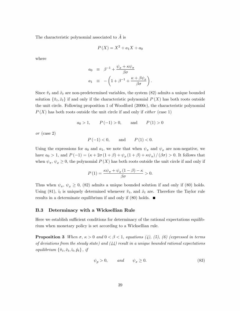
The characteristic polynomial associated to ~A is

P (X) = X2 + a1X + a0

where

a0 ´ ¯¡1 +Ãx + ·Ã¼¯¾

a1 ´ ¡µ1 + ¯¡1 +

·+ ¯Ãx¯¾

¶:

Since ¼t and xt are non-predetermined variables, the system (82) admits a unique bounded

solution f¼t; xtg if and only if the characteristic polynomial P (X) has both roots outsidethe unit circle. Following proposition 1 of Woodford (2000c), the characteristic polynomial

P (X) has both roots outside the unit circle if and only if either (case 1)

a0 > 1; P (¡1) > 0; and P (1) > 0

or (case 2)

P (¡1) < 0; and P (1) < 0:

Using the expressions for a0 and a1; we note that when ü and Ãx are non-negative, we

have a0 > 1; and P (¡1) = (·+ 2¾ (1 + ¯) + Ãx (1 + ¯) + ·Ã¼) = (¯¾) > 0: It follows thatwhen ü; Ãx ¸ 0; the polynomial P (X) has both roots outside the unit circle if and only if

P (1) =·Ã¼ + Ãx (1¡ ¯)¡ ·

¯¾> 0:

Thus when ü; Ãx ¸ 0; (82) admits a unique bounded solution if and only if (80) holds.

Using (81), {t is uniquely determined whenever ¼t; and xt are. Therefore the Taylor rule

results in a determinate equilibrium if and only if (80) holds.

B.3 Determinacy with a Wicksellian Rule

Here we establish su¢cient conditions for determinacy of the rational expectations equilib-

rium when monetary policy is set according to a Wicksellian rule.

Proposition 3 When ¾; · > 0 and 0 < ¯ < 1; equations (4), (5), (6) (expressed in termsof deviations from the steady state) and (44) result in a unique bounded rational expectations

equilibrium f¼t; xt; {t; ptg ; if

Ãp > 0; and Ãx ¸ 0: (83)

39

Proof. First recall that using (44) to substitute for {t in the intertemporal IS equation,we can rewrite (4), (5) and (6) (expressed in terms of hatted variables) in matrix form as:

Et

264 ¼t+1xt+1

pt

375 = A264 ¼t

xt

pt¡1

375+ a" retut

#(84)

where the matrix A is given by

A =

2664¯¡1 ¡·¯¡1 0

¾¡1¡Ãp ¡ ¯¡1

¢ ³1 + ¾¡1

³·¯ + Ãx

´´Ãp¾

¡1

1 0 1

3775 :The characteristic polynomial associated to A is

P (X) = X3 +A2X2 +A1X +A0

where

A0 = ¡¾ + Ãx¯¾

A1 =·+ ¾¯ + 2¾ + Ãx¯ + ·Ãp + Ãx

¯¾

A2 = ¡2¾¯ + ¾ + ·+ Ãx¯¯¾

:

The system (84) results in a determinate equilibrium if and only if the characteristic polyno-

mial P (X) admits two roots outside and one root inside the unit circle. Using proposition

2 of Woodford (2000c), P (X) has one root inside the unit circle and two roots outside if

P (1) > 0; P (¡1) < 0; and jA2j > 3:

Assume that Ãp and Ãx satisfy (83). This implies

P (1) =·

¯¾Ãp > 0

P (¡1) = ¡2·+ 4¾ (1 + ¯) + ·Ãp + 2(1 + ¯)Ãx¯¾

< 0

jA2j = 2 + ¯¡1 +·+ Ãx¯

¯¾> 3:

Hence P (X) has exactly 2 roots outside the unit circle, and (84) results in a determinate

equilibrium.

40

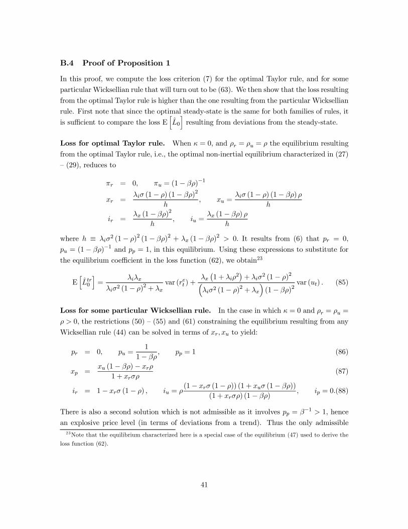
B.4 Proof of Proposition 1

In this proof, we compute the loss criterion (7) for the optimal Taylor rule, and for some

particular Wicksellian rule that will turn out to be (63). We then show that the loss resulting

from the optimal Taylor rule is higher than the one resulting from the particular Wicksellian

rule. First note that since the optimal steady-state is the same for both families of rules, it

is su¢cient to compare the loss EhL0iresulting from deviations from the steady-state.

Loss for optimal Taylor rule. When · = 0; and ½r = ½u = ½ the equilibrium resulting

from the optimal Taylor rule, i.e., the optimal non-inertial equilibrium characterized in (27)

– (29), reduces to

¼r = 0; ¼u = (1¡ ¯½)¡1

xr =¸i¾ (1¡ ½) (1¡ ¯½)2

h; xu =

¸i¾ (1¡ ½) (1¡ ¯½)½h

ir =¸x (1¡ ¯½)2

h; iu =

¸x (1¡ ¯½) ½h

where h ´ ¸i¾2 (1¡ ½)2 (1¡ ¯½)2 + ¸x (1¡ ¯½)2 > 0: It results from (6) that pr = 0;

pu = (1¡ ¯½)¡1 and pp = 1; in this equilibrium. Using these expressions to substitute forthe equilibrium coe¢cient in the loss function (62), we obtain23

EhLtr0

i=

¸i¸x

¸i¾2 (1¡ ½)2 + ¸xvar (ret ) +

¸x¡1 + ¸i½2

¢+ ¸i¾2 (1¡ ½)2³

¸i¾2 (1¡ ½)2 + ¸x´(1¡ ¯½)2

var (ut) : (85)

Loss for some particular Wicksellian rule. In the case in which · = 0 and ½r = ½u =

½ > 0; the restrictions (50) – (55) and (61) constraining the equilibrium resulting from any

Wicksellian rule (44) can be solved in terms of xr; xu to yield:

pr = 0; pu =1

1¡ ¯½; pp = 1 (86)

xp =xu (1¡ ¯½)¡ xr½

1 + xr¾½(87)

ir = 1¡ xr¾ (1¡ ½) ; iu = ½(1¡ xr¾ (1¡ ½)) (1 + xu¾ (1¡ ¯½))

(1 + xr¾½) (1¡ ¯½) ; ip = 0:(88)

There is also a second solution which is not admissible as it involves pp = ¯¡1 > 1; hencean explosive price level (in terms of deviations from a trend). Thus the only admissible23Note that the equilibrium characterized here is a special case of the equilibrium (47) used to derive the

loss function (62).

41

solution is (86) – (88). Consider now an equilibrium in which xr and xu satisfy

xr =¸i¾ (1¡ ½)

¸i¾2 (1¡ ½)2 + ¸x(89)

xu = ¸i¾½

³¸i¾

2 (1¡ ½)2 + ¸x´¯¡1¡ ¯½2¢¡ ¸x½ (1¡ ¯)

(1¡ ¯½)¢ ; (90)

where

¢ ´³¸i¾

2 (1¡ ½)2 + ¸x´¡¸i¾

2¡1¡ ¯½2¢ (1¡ ¯½) + ¸x (1 + ¯½)¢ ;

and where (86) – (90) are used to compute the remaining coe¢cients. The latter are given

by (86) and

xp = ¡¸i¾½³¸i¾

2 (1¡ ½)2 + ¸x´ ¡1¡ ¯½2¢ (1¡ ¯)

¢

ir =¸x

¸i¾2 (1¡ ½)2 + ¸xiu = ½¸x

¸i¾2¡1¡ ¯½2¢ (1¡ ½) + ¸x (1 + ¯½)

(1¡ ¯½)¢ip = 0

Expressions (89) and (90 do in general not correspond to the values of xr and xu that

would minimize the loss criterion (62). (In fact they would minimize (62) in the special case

­u = 0:) As a result this equilibrium is not the optimal equilibrium that might be obtained

with a Wicksellian rule. We focus here on a suboptimal equilibrium because it is easier to

characterize analytically. We will call this equilibrium a “quasi-optimal equilibrium”. One

implication of course is that the resulting loss, EhLqwr0

i; cannot be smaller than the one

obtained in the optimal equilibrium, EhLwr0

i; so that

EhLqwr0

i¸ E

hLwr0

i:

The Wicksellian rule of the form (44) that implements this quasi-optimal equilibrium is

obtained by using (59) and (60). Substituting for the above equilibrium coe¢cients in (59)

and (60) yields:

Ãp =½¸x (1¡ ¯)

¡1¡ ¯½2¢

(1¡ ½) (¸i¾2 (1¡ ¯½2) (1¡ ¯½) + ¸x (1 + ¯½))Ãx =

¸x¸i¾ (1¡ ½) :

The Wicksellian rule considered is therefore (63). Notice that since Ãp > 0 and Ãx > 0;

it follows from proposition 3 (in Appendix B.3) that this rule results in a unique bounded

equilibrium.

42

Next, substituting the above equilibrium coe¢cients in the loss criterion (62), we obtain

EhLqwr0

i=

¡¸xx

2r + ¸ii

2r

¢var (ret )

+

µ1

(1¡ ¯½)2 + ¸xµx2u + 2xuxp

¯½

(1¡ ¯½)2 + x2p

¯ (1 + ¯½)

(1¡ ¯½)3 (1¡ ¯)

¶+ ¸ii

2u

¶var (ut)

=¸i¸x

¸i¾2 (1¡ ½)2 + ¸xvar (ret )

+

Ã1

(1¡ ¯½)2 + ¸i¸x½2¸i¾

2¯ (1¡ ½)2 ¡1¡ ¯½2¢+ ¸x ¡1¡ ¯2½2¢(1¡ ¯½)3¢

!var (ut) (91)

Comparing the losses. Substracting …nally (91) from (85), we obtain after some alge-

braic manipulations:

EhLtr0

i¡ E

hLqwr0

i=

¸x¸2i ¾

2(1¡¯½2)2(1¡¯)½2(1¡¯½)(¸2i¾4(1¡¯½2)(1¡¯½)(1¡½)2+¸i¾2¸x(½2(1¡¯)(1¡¯½)+2(1¡¯½2)(1¡½))+¸2x(1+¯½))

> 0:

Thus

EhLtr0

i> E

hLqwr0

i¸ E

hLwr0

i;

which completes the proof. ¥

43

Table 1: “Calibrated” Parameter values

Structural parameters

¯ ¾ ·

0:99 0:1571 0:0238

Shock processes

½r ½u var (ret ) var (ut)

0:35 0:35 13:8266 0:1665

Loss function

¸x ¸i

0:048 0:236

44

Table 2: Statistics and Optimal Policy Rules

Statistics Coefficients of optimal policy ruleV[π ] V[x ] V[i ] V[p ] E[L 0] p t π t x t x t- 1 i t- 1 i t- 2

Optimal Plan / Optimal Ruleρ r = 0 ρ u = 0 0.157 10.215 0.983 0.938 0.883 -- 0.641 0.325 -0.325 2.163 -1.010

ρ u = 0.35 0.192 10.994 0.983 0.951 0.956 -- 0.641 0.325 -0.325 2.163 -1.010ρ u = 0.9 0.195 20.057 0.983 1.098 1.397 -- 0.641 0.325 -0.325 2.163 -1.010

ρ r = 0.35 ρ u = 0 0.217 11.056 1.922 2.727 1.206 -- 0.641 0.325 -0.325 2.163 -1.010ρ u = 0.35 0.252 11.835 1.922 2.740 1.279 -- 0.641 0.325 -0.325 2.163 -1.010ρ u = 0.9 0.255 20.898 1.922 2.887 1.720 -- 0.641 0.325 -0.325 2.163 -1.010

ρ r = 0.9 ρ u = 0 0.487 5.196 6.765 46.597 2.337 -- 0.641 0.325 -0.325 2.163 -1.010ρ u = 0.35 0.522 5.975 6.765 46.610 2.410 -- 0.641 0.325 -0.325 2.163 -1.010ρ u = 0.9 0.525 15.038 6.766 46.757 2.851 -- 0.641 0.325 -0.325 2.163 -1.010

Optimal Non-Inertial Plan / Optimal Taylor Rulesρ r = 0 ρ u = 0 0.269 13.495 2.030 1.680 1.401 -- 0.641 0.325 -- -- --

ρ u = 0.35 0.391 13.957 2.233 4.224 1.593 -- 1.291 0.263 -- -- --ρ u = 0.9 0.144 30.354 2.159 3.217 2.122 -- 3.658 0.038 -- -- --

ρ r = 0.35 ρ u = 0 0.358 9.989 6.747 3.631 2.435 -- 0.888 0.694 -- -- --ρ u = 0.35 0.479 10.451 6.949 6.175 2.627 -- 1.724 0.572 -- -- --ρ u = 0.9 0.233 26.848 6.876 5.168 3.156 -- 5.041 0.089 -- -- --

ρ r = 0.9 ρ u = 0 0.500 0.529 10.437 39.175 2.993 -- -1.743 -3.222 -- -- --ρ u = 0.35 0.622 0.991 10.640 41.719 3.185 -- -2.575 -2.495 -- -- --ρ u = 0.9 0.375 17.388 10.566 40.712 3.714 -- -5.108 -0.283 -- -- --

Optimal Wicksellian Rulesρ r = 0 ρ u = 0 0.122 13.923 1.237 0.008 1.087 1.997 -- 0.182 -- -- --

ρ u = 0.35 0.146 15.191 1.294 0.015 1.186 1.383 -- 0.228 -- -- --ρ u = 0.9 0.142 24.466 1.391 0.090 1.653 0.853 -- 0.274 -- -- --

ρ r = 0.35 ρ u = 0 0.149 15.898 2.646 0.013 1.543 2.872 -- 0.139 -- -- --ρ u = 0.35 0.161 17.597 2.778 0.018 1.669 2.338 -- 0.201 -- -- --ρ u = 0.9 0.096 28.790 2.761 0.012 2.140 3.323 -- 0.140 -- -- --

ρ r = 0.9 ρ u = 0 0.158 7.072 10.459 0.089 2.973 2.613 -- 0.134 -- -- --ρ u = 0.35 0.166 8.239 10.699 0.102 3.093 2.426 -- 0.241 -- -- --ρ u = 0.9 0.110 18.822 10.779 0.094 3.567 2.626 -- 0.259 -- -- --

Estimated Historical Ruleρ r = 0 ρ u = 0 0.178 10.531 1.313 0.833 0.997 -- 0.424 0.297 -0.032 1.160 -0.430

ρ u = 0.35 0.330 10.639 1.351 3.586 1.164 -- 0.424 0.297 -0.032 1.160 -0.430ρ u = 0.9 5.182 13.019 5.078 555.455 7.012 -- 0.424 0.297 -0.032 1.160 -0.430

ρ r = 0.35 ρ u = 0 0.215 11.941 2.961 1.218 1.492 -- 0.424 0.297 -0.032 1.160 -0.430ρ u = 0.35 0.367 12.049 2.999 3.972 1.659 -- 0.424 0.297 -0.032 1.160 -0.430ρ u = 0.9 5.219 14.429 6.726 555.841 7.507 -- 0.424 0.297 -0.032 1.160 -0.430

ρ r = 0.9 ρ u = 0 3.080 9.485 21.954 317.172 8.728 -- 0.424 0.297 -0.032 1.160 -0.430ρ u = 0.35 3.232 9.592 21.993 319.926 8.895 -- 0.424 0.297 -0.032 1.160 -0.430ρ u = 0.9 8.084 11.973 25.719 871.794 14.743 -- 0.424 0.297 -0.032 1.160 -0.430

Notes: The gray cases indicate that the policy rule results in an indeterminate equilibriumThe estimated historical rule refers to Judd and Rudebusch (1998).

�����������������������������������������������������������������������������������������������������������������������������������������������������������������������������

�����������������������������������������������������������������������������������������������������������������������������������������������������������������������������

�����������������������������������������������������������������������������������������������������������������������������������������������������������������������������

�����������������������������������������������������������������������������������������������������������������������������������������������������������������������������

�����������������������������������������������������������������������������������������������������������������������������������������������������������������������������

�����������������������������������������������������������������������������������������������������������������������������������������������������������������������������

�����������������������������������������������������������������������������������������������������������������������������������������������������������������������������

�����������������������������������������������������������������������������������������������������������������������������������������������������������������������������

�����������������������������������������������������������������������������������������������������������������������������������������������������������������������������

����������������������������������������������������������������������������������������������������������������������

������������������������������������������������������������������������������������������������������������������������������������������������������������������������������������������������������������������������������������

�����������������������������������������������������������������������������������������������������������������������������������������������������������������������������

����������������������������������������������������������������������������������������������������������������������������������

����������������������������������������������������������������������������������������������������������������������������������

����������������������������������������������������������������������������������������������������������������������������������

����������������������������������������������������������������������������������������������������������������������������������

����������������������������������������������������������������������������������������������������������������������������������

����������������������������������������������������������������������������������������������������������������������������������

����������������������������������������������������������������������������������������������������������������������������������

����������������������������������������������������������������������������������������������������������������������������������

����������������������������������������������������������������������������������������������������������������������������������

��������������������������������������������������������������������������������������������������������������������������������������������������������������������������������������������������������������������������������������������������������������������

����������������������������������������������������������������������������������������������������������������������������������

Figure 1a: Shock to re (ρr = 0)

___ optimal plan _ _ optimal non−inertial plan _._ optimal Wicksellian rule

0 1 2 3 4 5 6 7 80

0.5

1Interest rate

0 1 2 3 4 5 6 7 8−0.1

−0.05

0

0.05

0.1Inflation

0 1 2 3 4 5 6 7 8−0.5

0

0.5

1Output gap

0 1 2 3 4 5 6 7 8−0.04

−0.02

0

0.02

0.04Price level

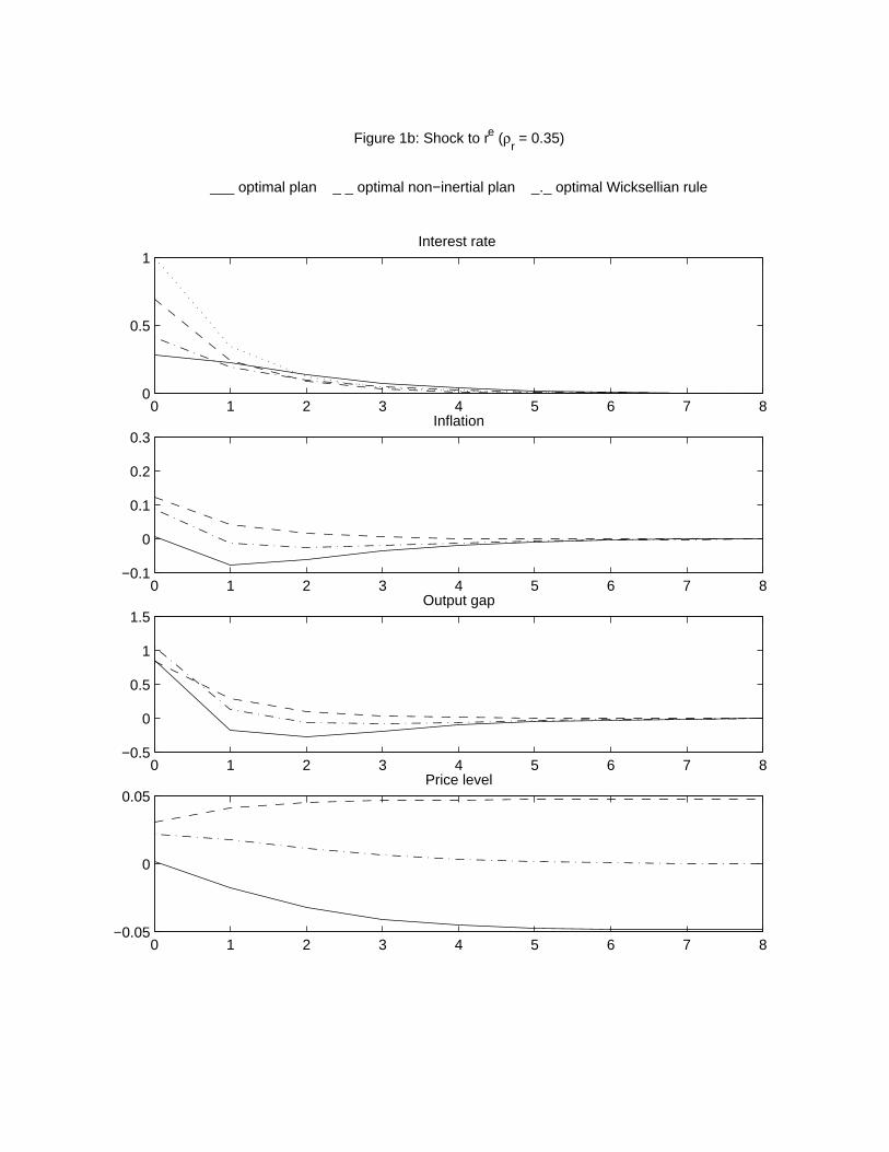
Figure 1b: Shock to re (ρr = 0.35)

___ optimal plan _ _ optimal non−inertial plan _._ optimal Wicksellian rule

0 1 2 3 4 5 6 7 80

0.5

1Interest rate

0 1 2 3 4 5 6 7 8−0.1

0

0.1

0.2

0.3Inflation

0 1 2 3 4 5 6 7 8−0.5

0

0.5

1

1.5Output gap

0 1 2 3 4 5 6 7 8−0.05

0

0.05Price level

Figure 1c: Shock to re (ρr = 0.9)

___ optimal plan _ _ optimal non−inertial plan _._ optimal Wicksellian rule

0 2 4 6 8 10 12 14 16 18 200

0.5

1Interest rate

0 2 4 6 8 10 12 14 16 18 20−0.2

−0.1

0

0.1

0.2Inflation

0 2 4 6 8 10 12 14 16 18 20−0.5

0

0.5

1

1.5Output gap

0 2 4 6 8 10 12 14 16 18 20−0.4

−0.2

0

0.2

0.4Price level

Figure 2a: Shock to u (ρu = 0)

___ optimal plan _ _ optimal non−inertial plan _._ optimal Wicksellian rule

0 1 2 3 4 5 6 7 80

0.2

0.4

0.6

0.8Interest rate

0 1 2 3 4 5 6 7 8−0.5

0

0.5

1Inflation

0 1 2 3 4 5 6 7 8−3

−2

−1

0Output gap

0 1 2 3 4 5 6 7 8−0.1

0

0.1

0.2

0.3Price level

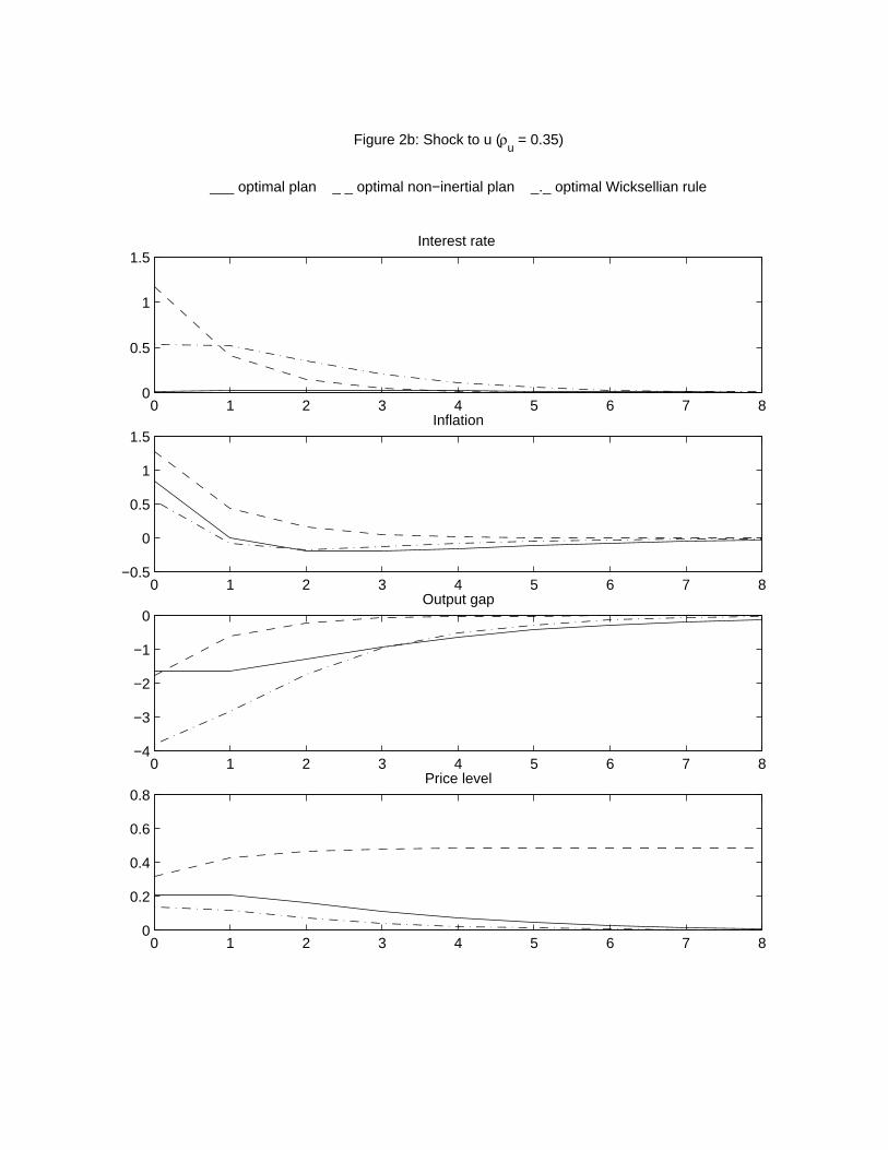
Figure 2b: Shock to u (ρu = 0.35)

___ optimal plan _ _ optimal non−inertial plan _._ optimal Wicksellian rule

0 1 2 3 4 5 6 7 80

0.5

1

1.5Interest rate

0 1 2 3 4 5 6 7 8−0.5

0

0.5

1

1.5Inflation

0 1 2 3 4 5 6 7 8−4

−3

−2

−1

0Output gap

0 1 2 3 4 5 6 7 80

0.2

0.4

0.6

0.8Price level

Figure 2c: Shock to u (ρu = 0.9)

___ optimal plan _ _ optimal non−inertial plan _._ optimal Wicksellian rule

0 2 4 6 8 10 12 14 16 18 20−0.5

0

0.5

1Interest rate

0 2 4 6 8 10 12 14 16 18 20−1

0

1

2Inflation

0 2 4 6 8 10 12 14 16 18 20−15

−10

−5

0Output gap

0 2 4 6 8 10 12 14 16 18 200

0.5

1Price level

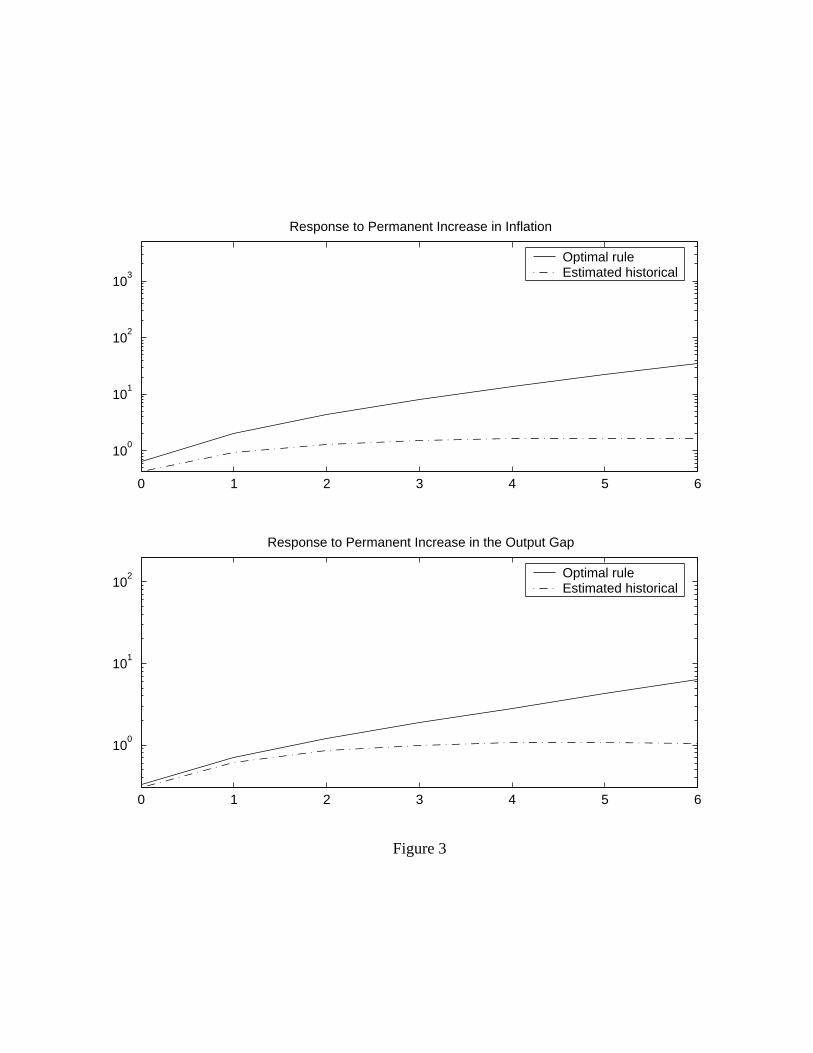
0 1 2 3 4 5 6

100

101

102

103

Response to Permanent Increase in Inflation

Optimal rule Estimated historical

0 1 2 3 4 5 6

100

101

102

Response to Permanent Increase in the Output Gap

Optimal rule Estimated historical

Figure 3

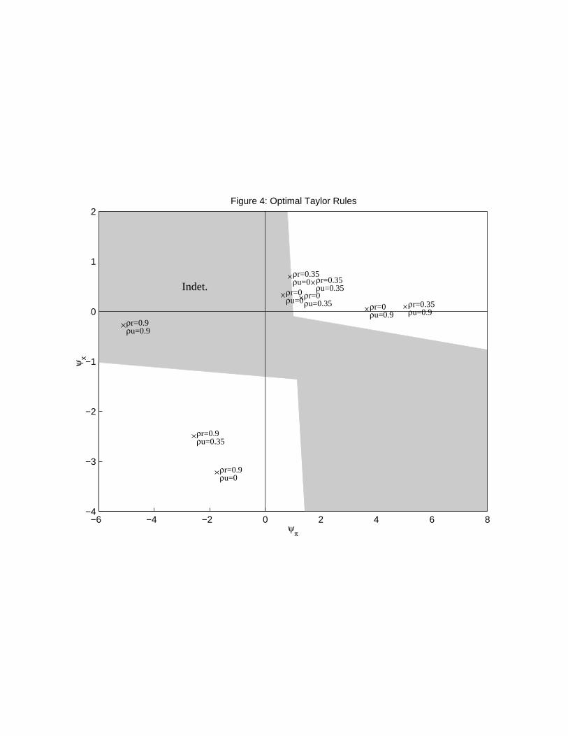
−6 −4 −2 0 2 4 6 8−4

−3

−2

−1

0

1

2

ψπ

ψx

Figure 4: Optimal Taylor Rules

ρr=0ρu=0

ρr=0.35ρu=0

ρr=0.9ρu=0

ρr=0ρu=0.35

ρr=0.35ρu=0.35

ρr=0.9ρu=0.35

ρr=0ρu=0.9

ρr=0.35ρu=0.9

ρr=0.9ρu=0.9

Indet.

0 0.5 1 1.5 2 2.5 3 3.5 40

0.05

0.1

0.15

0.2

0.25

0.3

0.35

0.4

0.45

0.5

ψp

ψx

Figure 5: Optimal Wicksellian Rules

ρr=0ρu=0

ρr=0.35ρu=0ρr=0.9

ρu=0

ρr=0ρu=0.35

ρr=0.35ρu=0.35

ρr=0.9ρu=0.35

ρr=0ρu=0.9

ρr=0.35ρu=0.9

ρr=0.9ρu=0.9

Fig

ure

6a: S

tatis

tics

and

Pol

icy

Rul

es a

s fu

nctio

ns o

f ρu

ρ r = 0

, var

(re )

= 1

3.82

66, v

ar(u

) =

0.1

6652

___

optim

al r

ule

_

_ op

timal

Tay

lor

rule

_

._ o

ptim

al W

icks

ellia

n ru

le

00.

51

0

0.1

0.2

0.3

0.4

0.5

V[π

]

00.

51

101520253035V

[x]

00.

51

0.51

1.52

2.53

V[i]

00.

51

0.51

1.52

2.5

E[L

0]

00.

51

02468V

[p]

00.

51

01234

ψπ

00.

51

0246810

ψp

00.

51

−0.

20

0.2

0.4

0.6

ψx

Fig

ure

6b: S

tatis

tics

and

Pol

icy

Rul

es a

s fu

nctio

ns o

f ρu

ρ r = 0

.35,

var

(re )

= 1

3.82

66, v

ar(u

) =

0.1

6652

___

optim

al r

ule

_

_ op

timal

Tay

lor

rule

_

._ o

ptim

al W

icks

ellia

n ru

le

00.

51

0

0.2

0.4

0.6

0.8

V[π

]

00.

51

101520253035V

[x]

00.

51

02468V

[i]

00.

51

1

1.52

2.53

3.5

E[L

0]

00.

51

0246810V

[p]

00.

51

0123456

ψπ

00.

51

02468

ψp

00.

51

−0.

20

0.2

0.4

0.6

0.8

ψx

Fig

ure

6c: S

tatis

tics

and

Pol

icy

Rul

es a

s fu

nctio

ns o

f ρu

ρ r = 0

.9, v

ar(r

e ) =

13.

8266

, var

(u)

= 0

.166

52

___

optim

al r

ule

_

_ op

timal

Tay

lor

rule

_

._ o

ptim

al W

icks

ellia

n ru

le

00.

51

0

0.2

0.4

0.6

0.8

V[π

]

00.

51

0510152025V

[x]

00.

51

6789101112V

[i]

00.

51

2

2.53

3.54

E[L

0]

00.

51

01020304050V

[p]

00.

51

−6

−5

−4

−3

−2

−1

ψπ

00.

51

2

2.53

3.54

4.5

ψp

00.

51

−4

−3

−2

−101

ψx

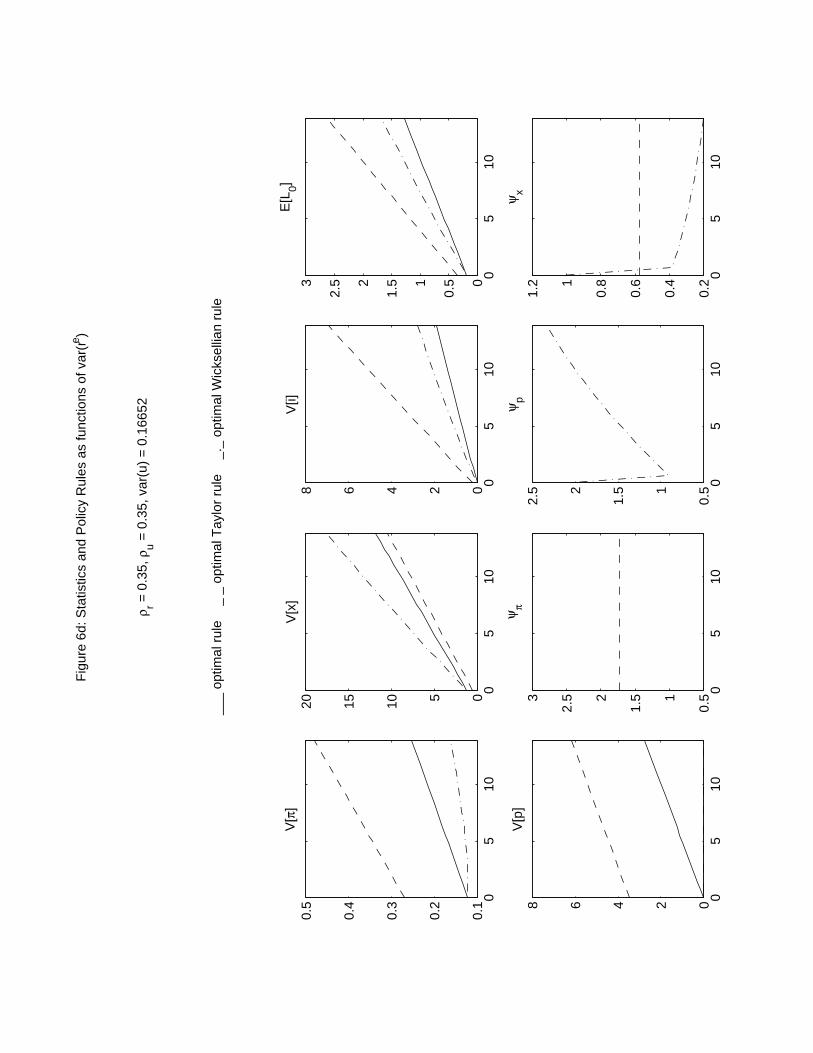
Fig

ure

6d: S

tatis

tics

and

Pol

icy

Rul

es a

s fu

nctio

ns o

f var

(re )

ρ r = 0

.35,

ρu =

0.3

5, v

ar(u

) =

0.1

6652

___

optim

al r

ule

_

_ op

timal

Tay

lor

rule

_

._ o

ptim

al W

icks

ellia

n ru

le

05

100.

1

0.2

0.3

0.4

0.5

V[π

]

05

1005101520

V[x

]

05

1002468

V[i]

05

100

0.51

1.52

2.53

E[L

0]

05

1002468

V[p

]

05

100.

51

1.52

2.53

ψπ

05

100.

51

1.52

2.5

ψp

05

100.

2

0.4

0.6

0.81

1.2

ψx

Fig

ure

6e: S

tatis

tics

and

Pol

icy

Rul

es a

s fu

nctio

ns o

f var

(u)

ρ r = 0

.35,

ρu =

0.3

5, v

ar(r

e ) =

13.

8266

___

optim

al r

ule

_

_ op

timal

Tay

lor

rule

_

._ o

ptim

al W

icks

ellia

n ru

le

00.

005

0.01

0

0.1

0.2

0.3

0.4

0.5

V[π

]

00.

005

0.01

81012141618V

[x]

00.

005

0.01

1234567V

[i]

00.

005

0.01

1

1.52

2.53

E[L

0]

00.

005

0.01

02468V

[p]

00.

005

0.01

0.51

1.52

2.53

ψπ

00.

005

0.01

2345678

ψp

00.

005

0.01

−0.

20

0.2

0.4

0.6

ψx

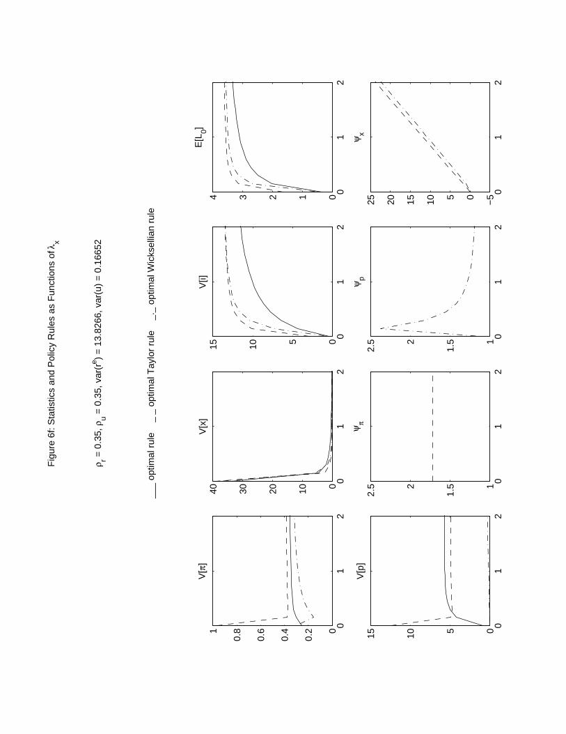
Fig

ure

6f: S

tatis

tics

and

Pol

icy

Rul

es a

s F

unct

ions

of λ

x

ρ r = 0

.35,

ρu =

0.3

5, v

ar(r

e ) =

13.

8266

, var

(u)

= 0

.166

52

___

optim

al r

ule

_

_ op

timal

Tay

lor

rule

_

._ o

ptim

al W

icks

ellia

n ru

le

01

20

0.2

0.4

0.6

0.81

V[π

]

01

2010203040

V[x

]

01

2051015

V[i]

01

201234

E[L

0]

01

2051015

V[p

]

01

21

1.52

2.5

ψπ

01

21

1.52

2.5

ψp

01

2−

50510152025

ψx