Optimal input design for nonlinear dynamical systems: a ...
148
Optimal input design for nonlinear dynamical systems: a graph-theory approach Theory and Applications PATRICIO E. VALENZUELA PACHECO Licentiate Thesis Stockholm, Sweden 2014
Transcript of Optimal input design for nonlinear dynamical systems: a ...

Optimal input design for nonlinear dynamical systems:
a graph-theory approach
Theory and Applications
PATRICIO E. VALENZUELA PACHECO
Licentiate ThesisStockholm, Sweden 2014

TRITA-EE 2014:059ISSN 1653-5146ISBN 978-91-7595-339-7
KTH Royal Institute of TechnologySchool of Electrical Engineering
Department of Automatic ControlSE-100 44 Stockholm
SWEDEN
Akademisk avhandling som med tillstånd av Kungliga Tekniska högskolan framläg-ges till offentlig granskning för avläggande av teknologie licentiatesexamen i elektrooch systemteknik fredagen den 21 november 2014 klockan 10.00 i Kollegiesalen,Kungliga Tekniska högskolan, Brinellvägen 8, Stockholm.
© Patricio E. Valenzuela Pacheco, October 2014
Tryck: Universitetsservice US AB

iii
Abstract
Optimal input design concerns the design of an input sequence to maxi-mize the information retrieved from an experiment. The design of the inputsequence is performed by optimizing a cost function related to the intendedmodel application. Several approaches to input design have been proposed,with results mainly on linear models. Under the linear assumption of themodel structure, the input design problem can be solved in the frequency do-main, where the corresponding spectrum is optimized subject to power con-straints. However, the optimization of the input spectrum using frequencydomain techniques cannot include time-domain amplitude constraints, whichcould arise due to practical or safety reasons.
In this thesis, a new input design method for nonlinear models is intro-duced. The method considers the optimization of an input sequence as arealization of the stationary Markov process with finite memory. Assuminga finite set of possible values for the input, the feasible set of stationary pro-cesses can be described using graph theory, where de Bruijn graphs can beemployed to describe the process. By using de Bruijn graphs, we can expressany element in the set of stationary processes as a convex combination ofthe measures associated with the extreme points of the set. Therefore, bya suitable choice of the cost function, the resulting optimization problem isconvex even for nonlinear models. In addition, since the input is restricted toa finite set of values, the proposed input design method can naturally handleamplitude constraints.
The thesis considers a theoretical discussion of the proposed input designmethod for identification of nonlinear output error and nonlinear state spacemodels. In addition, this thesis includes practical applications of the methodto solve problems arising in wireless communications, where an estimate ofthe communication channel with quantized data is required, and applicationoriented closed-loop experiment design, where quality constraints on the iden-tified parameters must be satisfied when performing the identification step.


Acknowledgements
The present work is the result of the support I received from many people. I wouldlike to start by expressing my profound gratitude to my supervisors, AssistantProfessor Cristian Rojas and Professor Håkan Hjalmarsson. You gave me the op-portunity to continue my studies towards a Ph.D. degree, and I learned from youmany important aspects to consider in research. During these years I enjoyed a lotthe work we do in the system identification group, and I am pretty sure that thiswill be the case for the coming years, with new exciting challenges waiting for us!
The present form of this thesis is the contribution from many people who vol-unteer to read it and provide many valuable suggestions. Many thanks to JohanDahlin, Christian Larsson, André Teixeira, Martin Jakobsson, and Håkan Tereliusfor the time you spent reading the first drafts of this thesis, and for the feedbackyou gave me to improve the document. I also want to thank the people who con-tributed to the articles that are part of this thesis. My profound gratitude also goesto Professor Thomas Schön, Professor Bo Wahlberg, Professor Brett Ninness, Dr.Juan Carlos Agüero, Dr. Boris Godoy, Johan Dahlin, and Afrooz Ebadat. Thankyou very much!
I want to thank also the administrators Anneli Ström, Hanna Holmqvist, KristinaGustafsson, Gerd Franzon, and Karin Karlsson for all the support I received fromyou to solve many different questions I came up with, and for the good times wespend during lunch (especially the episodes of Lunch with Hanna) and fika, I reallyappreciate that.
During my time in the Department I met many nice people, that contributesto make our working place even more enjoyable. I appreciate every conversationwe have had, and all your support through these years. I would like to express mygratitude to all the people in the Department of Automatic Control, especially toMohamed Rasheed Abdalmoaty, Mariette Annergren, Per Hägg, Christian Lars-son, Niklas Everitt, Niclas Blomberg, Giulio Bottegal, Afrooz Ebadat, RiccardoSven Risuleo, and Miguel Ramos for all the good times we have spent workingtogether in the system identification group; Martin Jakobsson, Kuo-Yun Liang,Marco Molinari, Olle Trollberg, André Teixeira, Sadegh Talebi, Pedro Lima, andDemia Della Penda for making our office a nice working place, and all the time weshared talking about non-research topics; Damiano Varagnolo, Themistoklis Char-alambous, Winston García, Farhad Farokhi, Euhanna Ghadimi, Bart Besselink,
v

vi
P.G. di Marco, Martin Andreasson, Meng Guo, Stefan Magureanu, Arda Aytekin,Valerio Turri, and Burak Demirel for many interesting conversations; and HåkanTerelius for all the funny times we have had (including running, of course). Thanksa lot to all of you!
During my stay in Sweden I met very nice people who are willing to help whenI need support. My profound gratitude goes to Mats and Awa Danielsson and theirfamily; and Fernando de Hoyos and Lupita Nava for all the good times we have hadin Stockholm. I am really indebted with you for all your love and support duringour stay in Sweden, thank you a lot!
I also want to deeply thank to the academics in the Department of ElectronicEngineering in my home university, Professors Mario Salgado, Eduardo Silva (restin peace) and Ricardo Rojas, for guiding me in my first steps in the research field,and for encouraging me to continue my studies towards a Ph.D. degree. Thank youvery much!
The step of doing a Ph.D. would not be possible without the support of manyfriends I met in Chile. I am really indebted with every one of you guys! My profoundgratitude goes specially to Claudia Cortez, Marisol Vera, Alfred Rauch, MauricioMoya, Cristian Carrasco, Felipe López, Sebastián “el testigo” Pulgar, Matías Gar-cía and Gabriela Leal, Nelson López and Marcela Cubillos, Ramón Delgado, RocíoGuerra and their daughters, Diego Carrasco, Pedro Riffo and Valeria Araya, IvánVelásquez, Verónica Contreras and their children, Francisco Arredondo and Lucre-cia Aedo, Stjpe Halat and Francisco Vargas. I really appreciate all the support Ireceived from all of you over the years, thank you very much!
Finally, I would like to thank all the support and love I received from my family,my parents and my siblings. Your support and love is the essential energy I needto cope with all the challenges I face in my life. I am deeply indebted to mywife Daniela Medina for accepting the challenge of moving from Chile, and for allthe love and support I receive from her every day, I love you! I am also reallygrateful to the love and support received from my parents Patricio Valenzuela andBrígida Pacheco, and my siblings Cristian (and his family), Alex and my little sisterClaudia. My parents in law Germán Medina and Magda Miranda and my sistersin law Valentina and Rosario have always been present, giving us love and supportthrough all these years. My gratitude goes also to Raúl Díaz, Teresa Ojeda andMauricio Díaz (rest in peace), who are beyond a friendship: they became part ofmy family, and their love is always present. Thank you very much!
¡Muchas gracias de corazón a todos!Patricio E. Valenzuela
Stockholm, Sweden. October 2014.

Contents
Contents vii
Glossary ix
Acronyms xi
1 Introduction 11.1 System identification . . . . . . . . . . . . . . . . . . . . . . . . . . . 21.2 Input design . . . . . . . . . . . . . . . . . . . . . . . . . . . . . . . . 111.3 Thesis outline and main contributions . . . . . . . . . . . . . . . . . 15
I Theory 19
2 Graph theory and stationary processes 212.1 Graph theory: basic concepts . . . . . . . . . . . . . . . . . . . . . . 212.2 De Bruijn graphs and stationary processes . . . . . . . . . . . . . . . 232.3 Generation of stationary sequences . . . . . . . . . . . . . . . . . . . 302.4 Conclusion . . . . . . . . . . . . . . . . . . . . . . . . . . . . . . . . 35
3 Input design for NOE models 373.1 Problem formulation . . . . . . . . . . . . . . . . . . . . . . . . . . . 383.2 Input design via graph theory . . . . . . . . . . . . . . . . . . . . . . 423.3 Reducible Markov chains . . . . . . . . . . . . . . . . . . . . . . . . . 443.4 Numerical examples . . . . . . . . . . . . . . . . . . . . . . . . . . . 443.5 Conclusion . . . . . . . . . . . . . . . . . . . . . . . . . . . . . . . . 52
4 Input design for nonlinear SSM 554.1 Problem formulation . . . . . . . . . . . . . . . . . . . . . . . . . . . 564.2 A review on SMC methods . . . . . . . . . . . . . . . . . . . . . . . 574.3 New input design method . . . . . . . . . . . . . . . . . . . . . . . . 674.4 Numerical examples . . . . . . . . . . . . . . . . . . . . . . . . . . . 714.5 Conclusion . . . . . . . . . . . . . . . . . . . . . . . . . . . . . . . . 73
vii

viii CONTENTS
II Applications 75
5 Input design for quantized systems 775.1 Input design problem . . . . . . . . . . . . . . . . . . . . . . . . . . . 785.2 Background on ML estimation . . . . . . . . . . . . . . . . . . . . . 805.3 Information matrix computation . . . . . . . . . . . . . . . . . . . . 865.4 Numerical example . . . . . . . . . . . . . . . . . . . . . . . . . . . . 885.5 Conclusion . . . . . . . . . . . . . . . . . . . . . . . . . . . . . . . . 90
6 Closed-loop input design 916.1 Preliminaries . . . . . . . . . . . . . . . . . . . . . . . . . . . . . . . 936.2 Input design for feedback systems . . . . . . . . . . . . . . . . . . . . 966.3 Numerical example . . . . . . . . . . . . . . . . . . . . . . . . . . . . 1036.4 Conclusion . . . . . . . . . . . . . . . . . . . . . . . . . . . . . . . . 108
7 Conclusions 109
A Algorithms for elementary cycles 115A.1 Preliminaries . . . . . . . . . . . . . . . . . . . . . . . . . . . . . . . 115A.2 Strong connected components of a graph . . . . . . . . . . . . . . . . 116A.3 Elementary cycles of a graph . . . . . . . . . . . . . . . . . . . . . . 117
B Convergence of the approximation of IF 121
C The EM algorithm 123C.1 The expectation-maximization algorithm . . . . . . . . . . . . . . . . 123C.2 EM algorithm: useful identities . . . . . . . . . . . . . . . . . . . . . 125
Bibliography 129

Glossary
δ(x) Dirac delta function at x = 0.(·)⊤ Transpose operator.#X Cardinality of the set X .det(·) Determinant operator.expx Exponential function: ex.λmin(·) Minimum eigenvalue.1X Indicator function: 1X = 1 if X is true; 0 otherwise.
erf(X ) Error function: 2√π
∫X e−u2
du.
supp(p) Support of p.tr· Trace operator., Matrix inequalities.q Time shift operator, q ut = ut+1.x1:N xkNk=1.P Cumulative distribution function (cdf).p Probability density function (pdf).E· Expectation operator.Cov(x) E
(x− Ex)(x− Ex)⊤.
χ2α(n) α-percentile of the χ2-distribution with n degrees of free-
dom.N (x, y) Normal distribution with mean x and variance y 0.AsN (x,M) Asymptotic normal distribution with mean x and covari-
ance M 0.P·|· Conditional probability measure.P· Probability measure.P Set of cdfs associated with stationary vectors utnm
t=1.PC Set of probability mass functions associated with stationary
vectors utnm
t=1.VPC
Set of all the extreme points of PC .E Set of edges.V Set of nodes.GV Directed graph with nodes in V .GCn n-dimensional de Bruijn graph derived from Cn.
ix

x GLOSSARY
Ar Set of ancestors of r.Dr Set of descendants of r.M Model set.Θ Set of feasible parameters.θ Parameter employed for estimation.θ0 True parameter in Θ.
θN Estimated parameter based on the data set ZN .yt|t−1(θ) Mean square optimal one-step ahead predictor given Zt−1.
S(θ) Score function:∂
∂θlog pθ(y1:N ).
ZN Data set composing of N samples.R+ x ∈ R : x > 0.Rn Set of n-dimensional vectors with real entries.Rr×s Set of r × s matrices with real entries.Z Set of integer numbers.

Acronyms
APF Auxiliary particle filter.AR Autoregressive.ARMA Autoregressive moving average.ARMAX Autoregressive moving average with exogenous input.ARX Autoregressive with exogenous input.
cdf Cumulative distribution function.CRLB Cramér-Rao lower bound.
EM Expectation maximization.
FIM Fisher information matrix.FIR Finite impulse response.FL Fixed-lag.
IS Importance sampling.
MA Moving average.MIMO Multiple input multiple output.ML Maximum likelihood.MPC Model predictive control.
NOE Nonlinear output error.NSSM Nonlinear state space model.
OE Output error.
pdf Probability density function.PEM Prediction error method.PF Particle filter.pmf Probability mass function.
xi

xii ACRONYMS
SIS Sequential importance sampling.SISO Single input single output.SMC Sequential Monte Carlo.SSM State space model.

Chapter 1
Introduction
Modeling is an important stage in many applications. By modeling we mean theprocess of obtaining a mathematical description for a given natural phenomenon(also called system). Examples include prediction of prices in finance [85], channelestimation in communication systems [88], and design of controllers in industrialprocesses [80].
We can distinguish two main approaches to modeling. The first approach con-siders the modeling of a natural phenomenon based on physical laws (e.g., the use ofthe Kirchhoff’s current and voltage laws to model an electrical circuit). The secondapproach is to model the natural phenomenon as a black box model (or gray boxmodel, if some physical insight for the model is taken into account) and identify themodel based on the input-output data from an experiment performed in the system(e.g., provide a voltage excitation to an electrical circuit, and measure the currentto obtain a model for the equivalent impedance). In this thesis we are interestedin the second approach, which is commonly referred to as system identification.
One key issue in system identification is the input sequence we provide to excitethe system. Since system identification requires input-output data, it is relevantto design an input excitation that maximizes the information in the experimentin a certain sense (e.g., optimizing a cost function related to the intended modelapplication). The process of designing an input sequence for system identificationis commonly referred to as input design, which is the focus of this thesis.
A distinction is made between the terms input design and experiment design.In experiment design, the choices include the definition of input and output signals,the measurement instants, the manipulated signals, and how to manipulate them(which is the focus of input design). It also includes signal conditioning (e.g., thechoice of presampling filters [59, Chapter 13]).
In this chapter, we provide some background on the theory of system identifi-cation and input design, which will be useful for the next chapters. In addition,this chapter also presents the main contributions of this work and the outline ofthe thesis.
1

2 CHAPTER 1. INTRODUCTION
ytSystemut
vmt
vt︷ ︸︸ ︷
Figure 1.1: Block diagram representing the concept of a system.
1.1 System identification
System identification concerns the modeling of a system based on input-outputdata collected from it. Quoting [59, Section 1.1], we can define a system as “anobject in which variables of different kinds interact and produce observable signals”.In this context, the inputs are the external stimuli affecting the system (whichare available to be manipulated by the user), and the outputs are the observablesignals of interest. In addition, the system can also be affected by disturbances,which are stimuli that cannot be controlled (but which could possibly be measured).Figure 1.1 depicts a block diagram with the concept of a system. In this figure,yt denotes the output, ut the input, vmt the measured disturbances, and vt thedisturbances.
As can be seen from the given definition of a system, the theory of systemidentification can be applied in a wide range of fields. In the following subsections,we will provide a brief discussion of the main elements and results in the theory ofsystem identification.
The basic entities
To build a model from data, we require three basic entities: a data set, a set ofcandidate models describing the relation between the input-output data (referred toas model structure), and an estimator to choose a model from the set of candidates(referred to as identification method).
Data set
In order to estimate a model, we require a set of input-output data from the sys-tem. This data set can also contain information regarding the measured distur-bances. Following the notation in Figure 1.1, the data set is defined as ZN :=yt, ut, vmt Nt=1.

1.1. SYSTEM IDENTIFICATION 3
Model structure
Given the data set ZN , we want to use it to estimate a model for the system.The model is normally constrained to a set containing the possible mathematicaldescriptions, which is called the model set. The choice of the model set is basedon prior information available about the system, on information obtained from thedata set using nonparametric techniques, or a combination of both approaches. Inthe next examples we illustrate some common choices for the model set.
Example 1.1 (Linear time invariant models) If the system is working locally aroundan equilibrium point, then it is reasonable to consider that it can be described by amodel in the set
M = yt = G(q; θ)ut +H(q; θ)et|θ ∈ Θ , (1.1)
where Θ ⊆ Rnθ is a set of parameters. G(q; θ) and H(q; θ) are rational functionsin the time shift operator q (i.e., q ut = ut+1), parameterized by θ. Here, etis a white noise sequence with zero mean and finite variance. In this case, thedisturbance vt in Figure 1.1 can be described as
vt = H(q; θ0)et , (1.2)
for some θ0 ∈ Θ. We notice that the system in Figure 1.1 is assumed to haveadditive output disturbances. Finally, since we do not have access to measure thedisturbance (or part of it), the signal vmt in Figure 1.1 is empty.
Remark 1.1 (Undermodeling) A common assumption on the model set M is thatthere exists at least one θ0 ∈ Θ such that the model evaluated at θ0 describes thetrue system. If this condition is not fulfilled, then we say that the system is under-modeled by M. In this thesis we assume that M contains the exact description ofthe system, i.e., there is no undermodeling.
Depending on the assumptions on G(q; θ) and H(q; θ), the model set of linearsystems in Example 1.1 can describe different structures, such as moving average(MA), autoregressive (AR), autoregressive with exogenous input (ARX), autore-gressive moving average (ARMA), and autoregressive moving average with exoge-nous input ARMAX [59].
Example 1.2 (Nonlinear state space models (NSSM)) Sometimes the linear as-sumption introduced in Example 1.1 is very restrictive. For example, the systemcould work in regions where the nonlinearities cannot be neglected.
There are several alternatives to model nonlinear systems. One of the mostgeneral model sets is given in terms of a nonlinear state space description [77]. Anonlinear state space model is defined as
M =
xt+1 = fθ(xt, ut, et)yt = gθ(xt, wt)
∣∣∣∣ θ ∈ Θ
, (1.3)

4 CHAPTER 1. INTRODUCTION
where Θ ⊆ Rnθ is a set of parameters as in Example 1.1. fθ and gθ are nonlinearfunctions parameterized by θ. In this example, et and wt are mutually inde-pendent white noise sequences, with zero mean and finite variance. In this case, vtin Figure 1.1 is composed by the processes et and wt, and the signal vmt is empty(as in Example 1.1).
We notice that the model set in Example 1.2 includes also linear time invariantmodels with static nonlinearities, known as Wiener-Hammerstein models [59]. An-other interesting model set included in Example 1.2 is described in the followingexample.
Example 1.3 (Nonlinear output error models (NOE)) A particular model set as-sociated with the nonlinear state space model in Example 1.2 is
M =
xt+1 = fθ(xt, ut)yt = hθ(xt) + wt
∣∣∣∣ θ ∈ Θ
. (1.4)
Notice that (1.4) can be obtained from (1.3) by setting et = 0 for all t, andgθ(xt, wt) = hθ(xt)+wt. The models in the set (1.4) will be referred to as nonlinearoutput error (NOE) models.
We must emphasize that the model sets introduced in the previous examples arenot the only ones existing in the literature. Indeed, it is possible to find model setswith time varying structure [59], neural networks [101], and models based on kernelestimators [67], among others. The results discussed in the following chapters willbe mainly focused on the model sets introduced in Examples 1.1-1.3.
Identification method
A natural question is how to select a model from a given model set M and a givendata set ZN . The goal is to choose the model from M that best explains thedata ZN in a given sense. The technique employed to choose a model from thestructures in M is referred to as the identification method. Several identificationmethods have been proposed in the literature, including, e.g., least squares [28],instrumental variables [78], and subspace techniques [93], among others.
In this thesis, we work with two identification methods:
1. The maximum likelihood method, and
2. the prediction error method.
The methods are described in the next subsections.

1.1. SYSTEM IDENTIFICATION 5
The maximum likelihood method
The maximum likelihood (ML) method is one of the most attractive identificationmethods due to its statistical properties [24]. The ML method is based on thedistribution of the data set y1:N := (y1, . . . , yN ), which is parameterized by θ ∈Θ. The objective is to find the estimated parameter θN that best explains themeasurements y1:N . If we define pθ(y1:N ) as the probability density function (pdf)
associated with y1:N , then the estimate θN obtained by the ML method is given by
θN = arg maxθ∈Θ
pθ(y1:N) . (1.5)
The expression (1.5) has an intuitive interpretation: θN ∈ Θ is such that theobserved event y1:N becomes “as likely as possible” [59].
For simplicity reasons, the logarithm of the probability density function (pdf)pθ(y1:N ) is usually maximized instead of pθ(y1:N ). This quantity is referred to asthe log-likelihood function. Due to the monotonicity of the logarithm function, thesolution
θN = arg maxθ∈Θ
log pθ(y1:N ) , (1.6)
is equal to the solution in (1.5). The expression (1.6) is usually prefered to (1.5)because products appearing in pθ(y1:N ) are converted into sums, and that the log-arithm removes exponentials (when the density pθ(y1:N ) is in the exponential class[9]) since logea = a. Another reason is that the use of logarithms results inalgorithms that are numerically more well-behaved [76].
To illustrate the computation of the log-likelihood function, we consider thefollowing example.
Example 1.4 (ML of a nonlinear SSM) Consider the nonlinear SSM described inExample 1.2. Due to the stochastic properties of the sequences et and wt, themodel set (1.3) can be rewritten as
M =
xt+1 ∼ pθ(xt+1|xt, ut)yt ∼ pθ(yt|xt)x1 ∼ pθ(x1)
∣∣∣∣∣∣θ ∈ Θ
, (1.7)
where “∼” denotes “distributed according to”, and pθ(xt+1|xt, ut), pθ(yt|xt) arethe conditional probability density functions of xt+1 and yt, conditioned on xt andut, respectively.
An important property associated with the stochastic models in (1.7) is theMarkov property, which means that the distribution of xt+1 and yt given xk, uktk=−∞equals their distribution given xt, ut.
The likelihood function can be computed using the definition of conditional prob-ability density functions as [69]
pθ(y1:N ) = pθ(y1)
N∏
t=2
pθ(yt|y1:t−1) . (1.8)

6 CHAPTER 1. INTRODUCTION
Taking the logarithm of (1.8), we obtain
log pθ(y1:N ) = log pθ(y1) +
N∑
t=2
log pθ(yt|y1:t−1) . (1.9)
From (1.9) we see that the logarithm of the likelihood function transforms the productof pdfs into a sum.
We use the Markov property associated with the model set (1.7) to compute thepdfs in (1.9) as
pθ(yt|y1:t−1) =
∫
Xt
pθ(yt|xt)pθ(xt|y1:t−1) dxt , (1.10)
pθ(xt|y1:t) =pθ(yt|xt)pθ(xt|y1:t−1)
pθ(yt|y1:t−1), (1.11)
pθ(xt+1|y1:t) =
∫
Xt
pθ(xt+1|xt, ut)pθ(xt|y1:t) dxt , (1.12)
where Xt denotes the set of values for xt. Equations (1.10)-(1.11) are known as themeasurement update, and equation (1.12) is known as the time update. Together,equations (1.10)-(1.12) can be employed to recursively compute the pdfs in the log-likelihood function (1.9).
Example 1.4 illustrates how the information available in the model set can beemployed to compute the log-likelihood function. It is important to emphasizethat, in general, equations (1.10)-(1.12) cannot be computed in closed form. Anexception is when the system is linear and Gaussian, where we can recover theexpressions for the Kalman filter [47] from (1.10)-(1.12). The reason is that theanalytic solutions of the integrals (1.10) and (1.12) are only available for specificcases. When a closed-form expression is not available, the optimization of (1.9)over Θ is highly complex. An approach to solve this issue has been proposed in[77], where particle methods are employed to numerically compute the expectation-maximization algorithm [20, 66] to maximize (1.9).
The prediction error method
The prediction error method (PEM) is another approach to find the best model inthe set M that explains the data ZN [59]. In this method, the estimated parameter
θN is obtained asθN = arg min
θ∈ΘVN (θ) , (1.13)
where
VN (θ) :=
N∑
t=1
ℓ(εt(θ)) , (1.14)

1.1. SYSTEM IDENTIFICATION 7
εt(θ) := yt − yt|t−1(θ) . (1.15)
Here yt|t−1(θ) denotes the mean square optimal one-step ahead predictor giveny1:t−1, which is computed as
yt|t−1(θ) := Eyt|y1:t−1 =
∫
Yt
yt pθ(yt|y1:t−1) dyt , (1.16)
and E· is the expectation operator. In (1.16) Yt denotes the set of values for yt,and the function ℓ(·) is an arbitrary and user chosen positive function (typicallydefined as a quadratic operator). We note that minimizing the prediction errors,εt(θ), makes sense since the models are normally employed for prediction, as incontrol system synthesis. Normally the systems are stochastic, which means thatthe output of the system at time t cannot be exactly determined by the data upto time t− 1. Therefore, it is valuable to know at time t− 1 what the output yt islikely to be in order to compute the appropriate control action [79].
The prediction error method has a number of benefits [60]:
• It can be applied to a wide spectrum of model parameterizations since onlyan expression for (1.16) is required.
• It gives models with excellent asymptotic properties, thanks to its kinshipwith the ML method (cf. Example 1.5 below).
• It can handle systems that operate in closed-loop (the input is partly de-termined via output feedback, when the data are collected) without addi-tional modifications to the method [27]. This property is also part of the MLmethod.
To illustrate the connection between PEM and the ML method, we introduce thefollowing example:
Example 1.5 (PEM and ML method) Consider a single output system that can bewritten as
yt = yt|t−1(θ0) + et , (1.17)
where et is white noise, Gaussian distributed with zero mean and variance σ2(θ0),and yt|t−1(θ0) given by (1.16). Under the previous assumption, the log-likelihoodfunction can be written as
log pθ(y1:N ) = −1
2
N∑
t=1
ε2t (θ) − N
2log σ2(θ) + c , (1.18)
where εt(θ) is defined in (1.15), and c is a constant independent of θ. If we assumethat εt(θ) and σ2(θ) are independently parameterized in θ, then we can maximize

8 CHAPTER 1. INTRODUCTION
over σ2(θ) to obtain an expression in terms of εt(θ). This allows to rewrite (1.18)as
log pθ(y1:N) = − 1
N
N∑
t=1
ε2t (θ) + c . (1.19)
If we compare (1.14) with (1.19), we see that PEM is retrieved from ML when etis Gaussian distributed white noise, and ℓ(εt(θ)) = N−1ε2
t (θ).
As in the previous subsection, equation (1.16) does not have a closed form expressionin general. Except for linear and specific nonlinear models, expression (1.16) canonly be computed numerically, e.g., using particle methods [77]. The next exampleshows the closed form expression for the optimal one-step ahead predictor in thelinear case.
Example 1.6 (Optimal one-step ahead predictor, linear case) Consider the modelset M introduced in Example 1.1. We will compute its optimal one-step aheadpredictor yt|t−1(θ), with θ ∈ Θ. To this end, we assume that limq→∞ H(q; θ) = I.Under this assumption, we can rewrite any model in M as
yt = G(q; θ)ut + (H(q; θ) − I)et + et . (1.20)
We notice that (H(q; θ)− I)et in (1.20) only contains information up to time t−1.Using (1.1) to compute et as a function of yt and ut, and inserting the result into(1.20), we obtain
yt = H−1(q; θ)G(q; θ)ut + (I −H−1(q; θ))yt + et . (1.21)
The first two terms in the right-hand side of the equality in (1.21) only depend onyk, ukt−1
k=1 if G is strictly proper (otherwise it is not a problem if ut is deter-ministic). In addition, since et is a white noise sequence, we have that the bestprediction of et given Zt−1 is Eet = 0. Therefore, the optimal one-step aheadpredictor associated with the model set in Example 1.1 is
yt|t−1(θ) = H−1(q; θ)G(q; θ)ut + (I −H−1(q; θ))yt . (1.22)
The expression (1.22) is a valid predictor if H−1(q; θ)G(q; θ) and H−1(q; θ) arestable [59, 79].
Remark 1.2 In Example 1.6, et cannot be predicted from Zt−1 since et is whitenoise. Due to this property, et is called the innovation of the process [59].
A useful predictor is introduced in the following example:
Example 1.7 (Optimal one-step ahead predictor, nonlinear output error models)Consider the nonlinear output error model introduced in Example 1.3. Since wt

1.1. SYSTEM IDENTIFICATION 9
is a white noise sequence with zero mean and finite variance, the optimal one-stepahead predictor associated with this model is
xt+1 = fθ(xt, ut) , (1.23a)
yt|t−1(θ) = hθ(xt) . (1.23b)
As it can be seen from the previous examples, PEM can be applied to find theestimated parameters θN for different models. The limitations of this method arethat an expression for yt|t−1(θ) must be available, and that the optimal one-stepahead predictor yt|t−1(θ) must be stable. For general nonlinear models, it mayhappen that yt|t−1(θ) is difficult to compute. To circumvent this issue, it is possibleto directly parameterize the model in terms of yt|t−1(θ) [59]. We notice that thedirect parametrization of yt|t−1(θ) can be seen as a nonlinear output error model,introduced in Example 1.3.
Asymptotic analysis
An important question regarding identification methods is their consistency, i.e., ifthe identification method can retrieve the model in M describing the true dynamicsof the system as N → ∞. Furthermore, we want to know if EθN = θ0, with
θ0 ∈ Θ defined as the parameter describing the true system. An estimator θNsatisfying EθN = θ0 is said to be unbiased.
On the other hand, we want to know the accuracy associated with the iden-tification method, i.e., the size of the variation of the identified model around itsexpected value. In this subsection we briefly discuss the consistency and accuracyof the parameter estimates θN as N → ∞. To start the analysis, we require thefollowing result [15, 59]:
Lemma 1.1 (Cramér-Rao bound) Let θN be an unbiased estimator of θ. Assumethat pθ0(y1:N ) (the pdf of y1:N ) is defined for all θ0 ∈ Θ, and that for all the valuesof y1:N where pθ(y1:N ) > 0, we have that
∂
∂θlog pθ(y1:N) , (1.24)
exists, and that ∣∣∣∣∂
∂θilog pθ(y1:N )
∣∣∣∣ (1.25)
is bounded above by an integrable function over the set defined for y1:N , for alli ∈ 1, . . . , nθ. In addition, suppose that y1:N may take values in a set whoseboundaries do not depend on θ. Then
E[θN − θ0
] [θN − θ0
]⊤ IeF −1 , (1.26)

10 CHAPTER 1. INTRODUCTION
where
IeF := E
∂
∂θlog pθ(y1:N )
∣∣∣∣θ=θ0
∂
∂θ⊤ log pθ(y1:N )
∣∣∣∣θ=θ0
∣∣∣∣∣u1:N
= −E
∂2
∂θ∂θ⊤ log pθ(y1:N )
∣∣∣∣θ=θ0
∣∣∣∣∣u1:N
. (1.27)
The result introduced in Lemma 1.1 states that the covariance of any unbiasedestimator θN cannot be smaller than the inverse of IeF , known as the Fisher infor-mation matrix. We notice that the computation of IeF requires the knowledge ofθ0 ∈ Θ, which implies that the exact value of IeF might not be available.
Remark 1.3 The quantity
S(θ) :=∂
∂θlog pθ(y1:N ) (1.28)
is usually known as the score function. The score function will be employed inChapter 4 to compute the Fisher information matrix for nonlinear state space mod-els.
To continue, we introduce the following definition:
Definition 1.1 (Efficient and Asymptotically efficient estimators) An estimator
θN is said to be efficient if expression (1.26) holds with equality for all N . If the ex-
pression (1.26) holds with equality for N → ∞, then θN is said to be asymptoticallyefficient.
The estimators obtained by the ML method and PEM (for a particular ℓ andGaussian innovations) are asymptotically efficient. From this perspective, it is
interesting to analyze how the estimator θN behave as N → ∞. The key result inthis area was introduced in [15, 97] for the asymptotic distribution of maximumlikelihood estimators obtained from independent observations:
Lemma 1.2 (Consistency and asymptotic distribution of ML estimators) Supposethat the random variables z1:N := ztNt=1 are independent and identically dis-tributed. Suppose also that the distribution of z1:N is given by pθ0 for some value
θ0 ∈ Θ. Then, as N → ∞, the random variable θN tends to θ0 with probability one,
and the random variable√N(θN − θ0
)converges in distribution to
√N(θN − θ0
)∈ AsN (0, IeF −1) , (1.29)
where IeF is given in Lemma 1.1.

1.2. INPUT DESIGN 11
The result introduced in Lemma 1.2 shows that, as N → ∞, the distribution ofthe random variable
√N(θN−θ0) tends to be normal with zero mean and covariance
matrix given by the Cramér-Rao bound. We notice that the result in Lemma 1.2is also true when the ML method is applied to dynamical systems under somemild conditions. Moreover, under technical conditions, the result in Lemma 1.2still holds for the estimator given by PEM when the white noise sequence et isGaussian and ℓ is a quadratic function [59].
Remark 1.4 The asymptotic distribution given in Lemma 1.2 does not necessarilyimply that
Cov(√NθN ) := N E
(θN − EθN)(θN − EθN)⊤
→ IeF −1 as N → ∞ .
(1.30)The result (1.30) requires more technical conditions on the stochastic processes act-ing on the system [59, Appendix 9B]. In this thesis we assume that those conditionsare fulfilled, which allows us to write
Cov(θN ) ≈ 1
NIeF −1 . (1.31)
As we can see in (1.31), the covariance matrix of an unbiased and asymptoticallyefficient estimator can be expressed in terms of the Cramér-Rao bound. One ques-tion that can arise at this point is if it is possible to shape the covariance matrix ofθN to improve the accuracy of the estimates. Indeed, since the Fisher informationmatrix (1.27) is conditioned on the input sequence u1:N , it is possible to shape the
covariance matrix of θN by designing u1:N , which is the main objective of inputdesign, described in the next section.
1.2 Input design
Optimal input design concerns the design of an excitation that maximizes the in-formation obtained in the data set ZN [14, 23, 33]. The maximization is usuallyperformed by optimizing a cost function related to the intended model applica-tion. Another standard choice for the cost function is a scalar number associatedwith the Fisher information matrix IeF [33, 45, 59]. We denote this cost functionh : Rnθ×nθ → R. To obtain convex optimization problems for the input designtechniques introduced in this thesis, h must satisfy the following definition [5]:
Definition 1.2 (Matrix concave function) A function f : Rr×r → R is calledmatrix concave if and only if, for every two matrices X, Y ∈ Rr×r in the positivesemidefinite cone, and for all λ ∈ [0, 1],
f(λX + (1 − λ)Y ) ≥ λf(X) + (1 − λ)f(Y ) . (1.32)
12 CHAPTER 1. INTRODUCTION
Table 1.1: Typical choices of h.
Optimality criterium h
A-optimality −tr
(·)−1
D-optimality log det(·)E-optimality λmin(·)L-optimality −tr
W (·)−1
According to Definition 1.2, some suitable choices for h are h = log det (D-criterion), h = −tr
(·)−1
(A-criterion), and h = λmin (E-criterion), among others.
Table 1.1 summarizes the definitions commonly used for the cost function h [49].By designing an optimal input sequence for identification we mean that, for a
given data length N , we optimize the accuracy for the parameter estimates in aprescribed sense. Since the cost function is associated with IeF , then by Remark 1.4we conclude that the maximization of IeF implies a reduction in the covariance
matrix of θN . In practical applications, input design allows to reduce the timeassociated with the experiment to obtain a prescribed accuracy. To see this, we notethat equation (1.31) implies that the covariance matrix of the parameter estimatesdecays as N−1. Furthermore, if IeF is optimized, then from equation (1.31) weconclude that we can reduce the number of samples required to achieve the desiredaccuracy for θN .
To illustrate the importance of input design, we consider the following example:
Example 1.8 (Fisher information matrix for an FIR model) Consider the finiteimpulse response (FIR) model
yt = θ1ut + θ2ut−1 + et , (1.33)
where θ =[θ1 θ2
]⊤ ∈ R2, and et is Gaussian white noise with zero mean andvariance λe. We are interested in identifying θ ∈ R2 by performing an experimentwith N = 2 samples and ut ∈ 1, 0. The Fisher information matrix IeF for themodel (1.33) is (assuming u0 6= 0)
IeF =1
λe
u21 + u2
2 u2 u1 + u1 u0
u2 u1 + u1 u0 u21 + u2
0
. (1.34)
From (1.34) we see that IeF depends on the input samples u0, u1, u2. Therefore,the choice of the input for the experiment is crucial to identify θ. For example, ifu1 = u2 = 1 and u0 = 1, the matrix IeF becomes
IeF =1
λe
[2 22 2
], (1.35)

1.2. INPUT DESIGN 13
which is singular. This implies that the parameter θ cannot be fully identified.Indeed, if we let the number of samples N → ∞, a constant input signal can onlybe employed to identify the DC gain of the model (1.33), which is the sum of theparameters. However, if in the previous case we choose u1 = 0, then IeF results in
IeF =1
λe
[1 00 1
], (1.36)
which is a nonsingular matrix. In conclusion, the design of u1, u2 to identify themodel (1.33) is an important step to obtain the desired results.
The optimal input design problem has been widely analyzed in the literature,with numerous results available. In the next subsection we provide a literaturereview with the main results in input design.
Literature review on input design
Most results in input design for dynamical systems have been developed for linearmodels [59]. The assumption of a linear model structure allows to use convexoptimization tools to solve the input design problem [32, 45, 57, 59, 74]. Severalmethods to design inputs for identification of linear systems have been reportedin the literature. In [74] the problem of input design for identification of linearsystems is addressed. The input sequence in [74] is designed by optimizing theexperiment for the worst case scenario defined by the model parameters, whichare assumed to lie in a given compact set. The optimal input design in [74] alsoconsiders energy (or power) constraints for the input sequence. Moreover, [74]shows a convex optimization algorithm that can be employed to solve a discretizedapproximation to the design problem. Another possibility to solve the optimalinput design problem is to employ linear matrix inequalities (LMI) to characterizeautocovariance functions associated with a feasible input spectrum [45, 57, 75, 96].In [45] the input design problem is solved in the frequency domain, where the inputspectrum is designed. To this end, [45] parameterizes the input spectrum usingrational basis functions. This allows to obtain a convex problem in the decisionvariables, where quality constraints on the identified model, and power constraintson the input signal can be included. A D-optimal multisine excitation is designedin [75], where the signal is employed to model physiological or electrochemicalphenomena from spectroscopy measurements. In [96] the optimal input design ispresented for finite impulse response (FIR) models, minimizing the uncertainty ofthe identified model while the variance of the input is kept as small as possible.A Markov chain approach is presented in [6, 7] to design inputs with amplitudeconstraints. The input sequence is assumed to be the output of a Markov chain,where the transition probability matrix is designed to maximize the informationretrieved from the experiment. However, the resulting problem is non-convex andnumerical optimization tools must be employed. We find the same problem for

14 CHAPTER 1. INTRODUCTION
time domain gradient-based schemes [32, 83], where only the convergence to localoptima can be guaranteed.
In recent years, the interest on input design has been extended from linear tononlinear systems. The main issue here is that most of the tools used for inputdesign for linear systems based on frequency domain techniques are no longer validfor the nonlinear case. One approach to input design for nonlinear systems is in-troduced in [42], where a linear systems perspective is considered. Based on aparticular nonlinear system, [42] raises the issue of obtaining a parametrization forthe input sequence that results in a tractable optimization. The main message in[42] is that it is possible to reuse some of the parameterizations of input sequencesfor linear models to the nonlinear case. Thus, it is possible to parameterize theinput sequence in terms of a probability density function describing a stationarystochastic process, but it is not straightforward to parameterize the input sequencein terms of its autocovariance function. In addition, [42] shows that it is possibleto use the sum-of-squares method to relax the input design problem for nonlinearmodels. Extensions to a class of FIR type systems is developed in [54], where acharacterization of probability density functions is employed. The assumption in[54] is that the input sequence is a realization of a stationary process with finitememory. Taking into account the structure of nonlinear FIR models, in [54] it isshown that the requirement of stationary process for the input can be combinedwith the model structure to obtain a convex optimization problem. Input designfor structured nonlinear identification is introduced in [94, 95], where the system isassumed to be an interconnection of linear systems and static nonlinearities. Theobjective in [94, 95] is to minimize the variance of the experiment, while achievingthe desired accuracy in the parameter estimates. It is shown in [94, 95] that theoptimization problem can be expressed in terms of the probability mass functioncharacterizing the input sequence. Moreover, [94, 95] shows that the resulting opti-mization problem is convex in the decision variables. Once the optimal probabilitymass function is obtained, [94, 95] generate an input realization using elementsfrom graph theory. An input design method for nonlinear state space models ispresented in [34], where a particle filter is used to approximate the cost functionassociated with the input design problem, which is optimized over a particular classof input vectors using stochastic approximation. In [34] it is assumed that the inputsequence is an autoregressive process filtering a white noise process with prescribedvariance, and the parameters of this process are optimized numerically. The meth-ods previously mentioned [34, 42, 54, 94, 95] are in general highly complex (usuallynon-convex problems, e.g., [34]) and are restricted to particular model structures(e.g., [42, 54, 94, 95]) or particular classes of input signals (e.g., white noise fil-tered through an ARX filter [34]). Moreover, except for the results in [6, 7, 54],the methods introduced cannot handle input design with amplitude constraints.Amplitude constraints can arise due to safety reasons or physical limitations in thesystem. Therefore, input design with amplitude constraints even for linear systemsalso requires further study.

1.3. THESIS OUTLINE AND MAIN CONTRIBUTIONS 15
1.3 Thesis outline and main contributions
In this thesis we present a novel approach to input design for nonlinear systems.The approach considers the design of input sequences for models with additivewhite noise at the output, and nonlinear state space models, extending the class ofnonlinear systems considered in [54]. The input is constrained to be a stationaryprocess with a finite set of possible values, and the associated probability massfunction (pmf) to have finite memory, i.e., a Markov chain of fixed order. There-fore, the problem is to find the pmf that maximizes the information obtained fromthe experiment, quantified as a scalar function of the information matrix. By usingnotions of graph theory, we can express the feasible set of pmfs as a convex combi-nation of the pmfs of the so-called prime cycles describing the vertices of the set.Since the prime cycles can be explicitly computed by known algorithms [46, 100],the optimization problem becomes easy to pose. Furthermore, for standard choicesof the cost function, the problem is convex even for nonlinear systems, which re-duces the computational complexity compared with the Markov chain approach in[6, 7]. Finally, since the input is restricted to a finite set of possible values, themethod naturally incorporates amplitude constraints.
The proposed input design method has proven to be an interesting solution topractical problems arising in the identification and estimation literature. As anillustration of the practical relevance of the proposed method, this thesis includestwo practical applications. First, we employ the input design technique for channelestimation with quantized output data. In this problem the quantized output dataintroduces nonlinear behavior, which restricts the techniques that can be employedto design an input sequence. Second, the proposed input design method is usedin closed-loop systems, where an external excitation is designed by minimizing theexperimental cost, subject to probabilistic constrains on the input and output ofthe plant, and simultaneously achieving a prescribed accuracy for the identifiedmodel. In this case, the cost function differs from the one employed in the previousdiscussion, since we aim to minimize the experimental cost instead of maximizingthe information in the experiment. However, the accuracy for the identified modelappears as a constraint, which guarantees the desired results in the solutions of theoptimization problem.
This thesis is organized in seven chapters, and 3 appendices. The chapters arestructured into two parts. In the first part, we discuss the theory employed by theinput design method, and the proposed solution to the problem of input design fornonlinear model structures. The second part describes the applications where themethod has been employed to improve the accuracy of the identified parameters.
The contents in each chapter are as follows:
Chapter 2: This chapter introduces notions from graph theory and their relationsto stationary processes. We show how the class of so-called de Bruijn graphscan be employed to describe the set of stationary processes with finite memoryand finite alphabet. The contents in this chapter are partially based on

16 CHAPTER 1. INTRODUCTION
P.E. Valenzuela, C.R. Rojas, and H. Hjalmarsson. A graph theoreti-cal approach to input design for identification of nonlinear dynamicalmodels. Accepted for publication, Automatica, 2014.
P.E. Valenzuela, C.R. Rojas, and H. Hjalmarsson. Optimal input designfor dynamic systems: a graph theory approach. In proceedings of the52nd Conference on Decision and Control (CDC), Florence, Italy, 2013.
Chapter 3: In this chapter a method for input design for nonlinear output errormodels is presented. The method considers the design of an input sequence asa realization of a stationary process with finite memory and finite alphabet,which allows us to use the theory introduced in Chapter 2 to obtain a tractableproblem. The results in this chapter are based on
P.E. Valenzuela, C.R. Rojas, and H. Hjalmarsson. A graph theoreti-cal approach to input design for identification of nonlinear dynamicalmodels. Accepted for publication, Automatica, 2014.
P.E. Valenzuela, C.R. Rojas, and H. Hjalmarsson. Optimal input designfor dynamic systems: a graph theory approach. In proceedings of the52nd Conference on Decision and Control (CDC), Florence, Italy, 2013.
Chapter 4: In this chapter an extension of the input design method to nonlinearstate space models is presented. The method considers the approach intro-duced in Chapter 2. In this chapter the information matrix is computed as thesample covariance of the score function, which is approximated using particlemethods. The results in this chapter are based on
P.E. Valenzuela, J. Dahlin, C.R. Rojas, and T.B. Schön. A graph/particle-based method for experiment design in nonlinear systems. In proceedingsof the 19th IFAC World Congress, Cape Town, South Africa, 2014.
Chapter 5: In this chapter we discuss an application of the input design methodto channel estimation with quantized output measurements. Using an avail-able expression for the information matrix of systems with quantized output,we use the input design method based on graph theory to design an inputsequence to identify the model. The results in this chapter are based on
B.I. Godoy, P.E. Valenzuela, C.R. Rojas, J.C. Agüero, and B. Ninness. Anovel input design approach for systems with quantized output data. Inproceedings of the 13th European Control Conference (ECC), Strasbourg,France, 2014.
Chapter 6: In this chapter an application of the input design method to closed-loop identification is presented. The objective is to design an input sequenceas a realization of a stationary process to identify a system operating in closedloop. The designed input sequence satisfies requirements on the informationretrieved from the experiment, and probabilistic bounds on the input and

1.3. THESIS OUTLINE AND MAIN CONTRIBUTIONS 17
output of the system. Using the proposed input design method, the resultingproblem is convex in the decision variables. The results in this chapter arebased on
A. Ebadat, P.E. Valenzuela, C.R. Rojas, H. Hjalmarsson, and B. Wahlberg.Applications oriented input design for closed-loop system identification:a graph-theory approach. Accepted for publication in the 53rd Confer-ence on Decision and Control (CDC), Los Angeles, United States, 2014.
Chapter 7: This chapter presents the conclusion of the thesis and future work onthe subject.
As a complement to the discussion in the chapters, 3 appendices are included:
Appendix A: We provide algorithms to compute the elementary cycles of a givengraph.
Appendix B: We provide the proof of the convergence for the approximation ofthe Fisher information matrix employed in Chapter 3.
Appendix C: We review the expectation-maximization algorithm, and derive someidentities that are useful in this thesis.


Part I
Theory
19


Chapter 2
Graph theory and stationary
processes
The results presented in this thesis rely on the connection between stochastic pro-cesses and graph theory. Therefore, the relation between these two concepts mustbe clarified before presenting the results in the coming chapters.
In this chapter, we introduce the elements from graph theory required to under-stand the discussions in the next chapters. We also define de Bruijn graphs, andhow they can be associated with stationary processes of finite memory. For thispurpose, we describe the set of stationary processes of a given memory as a convexcombination of the measures associated with the prime cycles of a de Bruijn graph[100].
Given an element in the set of stationary processes with finite memory, we wantto sample a realization with the prescribed distribution. In this chapter, we alsoprovide a novel method to obtain samples from a given probability measure thatdescribes the stationary distribution of a Markov chain.
2.1 Graph theory: basic concepts
In this section we provide a number of definitions for the graph theory conceptsemployed in the next chapters. Our notation follows that of [46, pp. 77].
Definition 2.1 (Directed graph) A directed graph GV = (V , E) is a pair consistingof a nonempty and finite set of vertices (called nodes) V and a set E of orderedpairs (vi, vj) of vertices vi, vj ∈ V called edges.
Remark 2.1 We note that Definition 2.1 does not impose restrictions over the setof vertices V. This allows to define V according to the requirement of the user.
Definition 2.2 (Path) A path in GV is a sequence of vertices
pvu = (v1 = v, v2, . . . , vk = u) ,
21

22 CHAPTER 2. GRAPH THEORY AND STATIONARY PROCESSES
such that (vi, vi+1) ∈ E for all i ∈ 1, . . . , k − 1.
Definition 2.3 (Cycle and elementary cycle) A cycle is a path in which the firstand last vertices are identical. A cycle is elementary if no vertex except the firstand last appears twice.
Definition 2.4 (Cyclic permutation) Consider two cycles puu and pvv in GV . Wesay that pvv is a cyclic permutation of puu if and only if there exists paths puv,and pvu such that pvv = (pvu, puv), where the first element in puv is removed, andpuu = (puv, pvu), where the first element in pvu is removed.
Definition 2.5 (Distinct elementary cycles) Two elementary cycles are distinct ifone is not a cyclic permutation of the other.
De Bruijn graphs
The results in this thesis are based on the class of directed graphs, called de Bruijngraphs [17]. Their definition is given below.
Definition 2.6 (de Bruijn graph) An n-dimensional de Bruijn graph of m symbolsC = s1, . . . , sm is a directed graph whose set of vertices V is given by
V = Cn = v1 = (s1, . . . , s1, s1), v2 = (s1, . . . , s1, s2), . . . ,
vm = (s1, . . . , s1, sm), vm+1 = (s1, . . . , s2, s1), . . . ,
vmn = (sm, . . . , sm, sm) , (2.1)
and whose set of directed edges E is
E = ((v1, r1, . . . , rn−1), (r1, r2, . . . , rn)) : v1, r1, . . . , rn ∈ C . (2.2)
Remark 2.2 According to Definition 2.6, an n-dimensional de Bruijn graph of msymbols is a directed graph representing overlaps between sequences of symbols. Ithas mn vertices, consisting of all possible sequences of length n derived from thegiven symbols of length n. The same symbol can appear multiple times in a sequence.Moreover, if one of the vertices can be expressed as another vertex by shifting allits symbols one place to the left and adding a new symbol at the end, then the latterhas a directed edge to the former vertex.
To illustrate Definition 2.6 we consider the following example:
Example 2.1 Consider a sequence ut with alphabet C = 0, 1. We are in-terested in deriving the de Bruijn graph associated with the possible transitions of(ut−1, ut) among its states in C2. In other words, we want to derive the possibletransitions when we move from (uk−1, uk) to (uk, uk+1). Table 2.1 contains allthe possible transitions between the elements in C2. We notice that the number ofpossible values of (uk, uk+1) for a given (uk−1, uk) is two, which is the number of

2.2. DE BRUIJN GRAPHS AND STATIONARY PROCESSES 23
(ut−1, ut)(1, 1)
(ut−1, ut)(0, 0)
(ut−1, ut)(1, 0)
(ut−1, ut)(0, 1)
Figure 2.1: The de Bruijn graph derived from C2, with C = 0, 1.
(ut−1, ut) (ut, ut+1)(0, 0) (0, 0), (0, 1)(0, 1) (1, 0), (1, 1)(1, 0) (0, 0), (0, 1)(1, 1) (1, 0), (1, 1)
Table 2.1: Transitions from (ut−1, ut) to (ut, ut+1), Example 2.1.
elements in C. This is due to the fact that the new element uk+1 belongs to C. Theresulting de Bruijn graph is depicted in Figure 2.1. We notice that the nodes aregiven by the elements of C2, and the edges correspond to the transitions presentedin Table 2.1.
Remark 2.3 We use GCn to denote the n-dimensional de Bruijn graph derivedfrom Cn.
2.2 De Bruijn graphs and stationary processes
In this section, we establish the connection between de Bruijn graphs and stationaryprocesses. Before proceeding, we introduce the following definitions:
Definition 2.7 (Cumulative distribution function) A function P : Cnm → R is acumulative distribution function (cdf) if and only if P (x1, . . . , xnm
) = PX1 ≤x1, . . . , Xnm
≤ xnm, where Xinm
i=1 are random variables, and P is a probabilitymeasure.

24 CHAPTER 2. GRAPH THEORY AND STATIONARY PROCESSES
Definition 2.8 (Stationary process) Consider the stochastic process ut. We saythat the process ut is stationary if and only if the cumulative distribution func-tions P associated with ut satisfy P (ui:i+k) = P (uj:j+k) for all integers i, j,k.
As we can see from Definition 2.8, a stationary process requires that all itsmarginal cumulative distribution functions (cdfs) are time invariant. The samedefinition can be restricted to the case of vectors:
Definition 2.9 (Stationary vectors) Consider the vector u1:nm. We say that the
vector u1:nmis stationary if and only if the cdf associated with u1:nm
satisfy
P (ui:i+k) = P (uj:j+k)
for all positive integers i, j, k satisfying 1 ≤ i ≤ j ≤ nm − k.
Stationary vectors
The concepts introduced in Section 2.1 can be employed to describe the set ofstationary processes. To this end, we consider the sequence ut, where ut ∈ C.Before continuing, we introduce the following definition:
Definition 2.10 (Probability mass function) A probability mass function (pmf) pis a probability measure whose support is a set with finite cardinality.
In this thesis we are interested in the case where ut is a stationary process.The description of ut is given in terms of the probability mass function (pmf),denoted by p. However, the description of ut as stationary process is intractablesince we need to define an infinite number of cumulative distribution functions (cf.Definition 2.8). To solve this issue, we use the following definitions:
Definition 2.11 (Extension of the cdf) Consider the cdf P (u1:nm). The exten-
sion of the cdf P (u1:nm) is defined as a Markov process ut of order nm, whose
stationary distribution is given by P (u1:nm).
Definition 2.12 (nm-dimensional projection [100, Theorem 1]) Consider the cdfP (u1:nm
). An nm-dimensional projection P (u1:nm) of P (u1:nseq) (nseq ≥ nm) is a
cdf P (u1:nm) associated with the stationary vector u1:nm
, which can be extended tothe stationary vector u1:nseq to define P (u1:nseq).
Based on Definitions 2.11-2.12, we assume the following:
Assumption 2.1 The stationary process ut is an extension of the stationarycumulative distribution function P (u1:nm
).

2.2. DE BRUIJN GRAPHS AND STATIONARY PROCESSES 25
Assumption 2.1 restricts the set of stationary processes ut to those that can beobtained as an extension of pdfs with a finite number of elements. This means thatP (u1:nseq) can be completely described by its nm-dimensional projection P (u1:nm
)for any nseq ≥ nm [100].
Given the restriction to the family of stationary processes we are interested in,we need to find a description for the set of pdfs associated with stationary processesof finite memory. For this end, we introduce the following result in terms of the cdf(whose proof follows from [100]):
Lemma 2.1 (Shift invariant property) Consider a stationary vector u1:nm. A cdf
P : Rnm → R is a valid cdf for u1:nmif and only if, for all z ∈ Rnm−1,
∫
v∈R
dP([v, z
])=
∫
v∈R
dP([
z, v]). (2.3)
Proof We know that P is a valid cdf for the stationary vector u1:nmif and only if
ui:i+kd∼ uj:j+k, for all positive integers i, j, k satisfying 1 ≤ i ≤ j ≤ nm −k. Here,
d∼ denotes equal in distribution.First we assume that P is a valid cdf for the stationary vector u1:nm
. This
implies that u1:nm−1d∼ u2:nm
, which is equivalent to the condition written in (2.3).
To prove the converse, we assume that (2.3) is true. Therefore, u1:nm−1d∼ u2:nm
issatisfied. Then for any k < nm, and by successive shifts, the marginal cdf P (u1:k)obtained from P (u1:nm
) satisfies
u1:kd∼ u2:k+1
d∼ u3:k+2 . . .d∼ unm−k+1:nm
, (2.4)
which implies that u1:nmhas a stationary distribution.
Lemma 2.1 states that a cdf P is associated with a stationary vector u1:nmif
and only if the cdf obtained by marginalizing over unmis equivalent to the one
obtained by marginalizing over u1. If a cdf P satisfies this property, then we saythat P is shift invariant.
The result introduced in Lemma 2.1 allows us to characterize the set of cdfsassociated with stationary vectors u1:nm
as
P :=
P : Rnm → R|P (x) ≥ 0, ∀x ∈ Rnm ;
P is monotone nondecreasing ;
limxi→∞
i∈1, ..., nmP (x1, . . . , xnm
) = 1,
∫
v∈R
dP([v, z
])=
∫
v∈R
dP([
z, v]), ∀z ∈ Rnm−1
. (2.5)

26 CHAPTER 2. GRAPH THEORY AND STATIONARY PROCESSES
We notice in (2.5) that the first three properties define a valid cdf. Introducingshift invariance as the fourth property in the set P , we obtain the projection of thecdfs of stationary sequences into the set of stationary vectors of length nm [100].
To exploit the relation between de Bruijn graphs and stationary vectors, weassume the following:
Assumption 2.2 The alphabet C is a finite set with cardinality nC.
In this thesis we restrict the analysis to the case when Assumption 2.2 is satisfied.Therefore, the set defined in Equation 2.5 will be restricted to the case of pmfs.Thus, the set we employ here is given by
PC := p : Cnm → R| p(x) ≥ 0, ∀x ∈ Cnm ;∑
x∈Cnm
p(x) = 1;
∑
v∈Cp([v, z
])=∑
v∈Cp([
z, v]), ∀z ∈ Cnm−1
. (2.6)
Remark 2.4 The cdfs associated with the elements in PC define a proper subset ofP.
We need to parameterize the elements of PC in a tractable manner. This issue isrelevant since in the next chapters we will optimize cost functions defined in termsof a stationary vector utnseq
t=1 , which are described as an extension of the pmfsp(u1:nm
) ∈ PC , where nm < nseq. A natural approach is to parameterize p(u1:nseq)in terms of a finite number of elements of PC , i.e., projections of stationary pmfs,since these elements can be extended to a full stationary pmf p(u1:nseq). Such aparameterization is described in the next subsection.
Parameterization of PC
To parameterize the elements of PC , we first notice that PC is a convex set, and,in particular, a polyhedron [72, pp. 170], since it is described by a finite numberof linear equalities and inequalities. Hence, any element of PC can be described asa convex combination of its extreme points [72, Corollaries 18.3.1 and 19.1.1]. Inother words, if we define VPC
:= wi, i = 1, ..., nV as the set of all the extremepoints of PC, then for all f ∈ PC we have
f =
nV∑
i=1
αiwi , (2.7)

2.2. DE BRUIJN GRAPHS AND STATIONARY PROCESSES 27
where αi ≥ 0, i ∈ 1, . . . , nV, and
nV∑
i=1
αi = 1 . (2.8)
The set VPCcan be characterized in a graph-theoretical manner. Since we have
restricted ut to belong to a finite alphabet C with nC elements (see Assumption 2.2),we notice that the set of possible values for (ut−nm+1, . . . , ut), Cnm , is composed ofnnm
C elements, which can be viewed as nodes in a graph. In addition, the transitionsbetween the elements in Cnm , as described by a stationary process of memory nm,are given by the possible values of ut+1 when we move from (ut−nm+1, . . . , ut) to(ut−nm+2, . . . , ut+1), for all integers t ≥ 0. The edges between the elements inCnm denote the possible transitions between the states, represented by the nodesof the graph. The resulting graph corresponds to a de Bruijn graph. To illustratethe transition among the nodes in the equivalent de Bruijn graph, we present thefollowing example:
Example 2.2 (Stationary vectors and de Bruijn graphs) Consider the de Bruijngraph depicted in Figure 2.1 in page 23, where nm = 2, and C = 0, 1. From thisfigure we can see that, if we are at node (0, 1) at time t, then we can only transitto node (1, 0) or (1, 1) at time t+ 1 (cf. Table 2.1 in page 23).
In order to describe the elements of VPC, the set of extreme points of PC , we
need the concept of prime cycles, whose definition is introduced below [100, pp.678]:
Definition 2.13 (Prime cycle) A prime cycle in a directed graph GV is an elemen-tary cycle whose set of nodes do not have a proper subset which is an elementarycycle.
The definition of prime cycle is illustrated in the next example.
Example 2.3 (Prime cycles and de Bruijn graphs) Consider again the de Bruijngraph depicted in Figure 2.1 in page 23. According to Definition 2.13, the cy-cle (0, 1), (1, 1), (1, 0), (0, 1) is not prime since it contains the elementary cycle(0, 1), (1, 0), (0, 1) in it. On the other hand, the elementary cycle (0, 1), (1, 0), (0, 1)is a prime cycle since it does not contain another elementary cycle.
To introduce the next theorem, we need the definition below.
Definition 2.14 (Descendants of an node in a de Bruijn graph) Consider a deBruijn graph GCn . For any x ∈ Cn, the set of descendants of x is defined as
Dx := v ∈ Cn : (x, v) ∈ E . (2.9)
We have the following result [100, Theorem 6]:

28 CHAPTER 2. GRAPH THEORY AND STATIONARY PROCESSES
Theorem 2.1 The prime cycles of the de Bruijn graph of a Markov process ofmemory nm are in one-to-one correspondence with the elements of VPC
, the setof extreme points of PC. In particular, each wi ∈ VPC
corresponds to a uniformdistribution whose support is the set of elements of a prime cycle.
Proof As an induction hypothesis, we assume that all measures in PC with lessthan k support points are mixtures of prime cycle measures. To start the induction,it is enough that the hypothesis is true when k = 1.
Let p ∈ PC have k points in its support. By Lemma 2.1, for any x ∈ supp(p),where supp(p) is the support of p, we have
0 < p(x) ≤∑
v∈Cp(v, x2, . . . , xnm
) =∑
v∈Cp(x2, . . . , xnm
, v) =∑
y∈Dx
p(y) . (2.10)
Equation (2.10) shows that for every x ∈ supp(p), there exists a y ∈ supp(p) forwhich y ∈ Dx. Because supp(p) is a finite set, this implies the existence of a cycleand hence a prime cycle in supp(p).
Let a := a1, . . . , ae be one such cycle, so that ai ∈ supp(p) for i ∈ 1, 2 . . . , e.Define
α := mini∈1, 2 ..., e
e p(ai) . (2.11)
By definition 0 < α ≤ 1. If α = 1 then p = pa, where pa is a measure assigningequal probability to the elements in a, and the induction is over. If α < 1, definethe measure
p′ :=p− αpa
1 − α. (2.12)
It is possible to verify that p′ is a probability measure. Moreover, p′ has at mostk − 1 support points, because
(1 − α)p′(ai) = p(ai) − αpa(ai) = p(ai) − mini∈1, 2 ..., e
e p(ai)1
e, (2.13)
which implies that p′(ai) = 0 for some i ∈ 1, 2 . . . , e. Finally, p′ ∈ PC becausep′ is a linear combination of the stationary measures p, and pa.
By the induction hypothesis, p′ is a mixture of prime cycle measures, and
p = α pa + (1 − α) p′ . (2.14)
This shows that any p ∈ PC is a mixture of prime cycle measures. It only remainsto show that all prime cycle measures are extreme points.
Let pa be a prime cycle measure. If pa is a mixture of stationary measures, bywhat has just been shown, pa is a mixture of prime cycle measures. For any pb inthat mixture, defined for a prime cycle b, we have supp(pb) ⊂ supp(pa). But a isprime cycle, so the only cycle contained in a is itself, and hence b = a. This showsthat pa is an extreme point.

2.2. DE BRUIJN GRAPHS AND STATIONARY PROCESSES 29
Theorem 2.1 says that we can describe all the elements in VPCby finding all the
prime cycles associated with the de Bruijn graph GCnm drawn from Cnm . To findall the prime cycles in GCnm , the de Bruijn graph with vertices in Cnm , we use thefollowing lemma.
Lemma 2.2 All the prime cycles associated with GCnm can be derived from theelementary cycles of GCnm−1 .
Proof For x, y ∈ Cnm−1 such that
(x2, . . . , xnm−1) = (y1, . . . , ynm−2) , (2.15)
define < x, y >∈ Cnm by
< x, y >:= (x1, x2, . . . , xnm−1, ynm−1) = (x1, y1, . . . , ynm−2, ynm−1) . (2.16)
For a cycle a := a1, . . . , ae, with ai ∈ Cnm−1 for all i ∈ 1, . . . , e, we create acycle a′ with elements in Cnm by defining
a′ := < a1, a2 >, < a2, a3 >, . . . , < ae, a1 > . (2.17)
Finally, we have that a′ in (2.17) is a prime cycle if and only if:
• < aj , aj+1 >∈ D<ai, ai+1> ⇔ i+ 1 = j,
• ai+1 = aj ⇔ i+ 1 = j,
• a is an elementary cycle.
Therefore, all the prime cycles in de Bruijn graph GCnm can be found by computingthe elementary cycles in the de Bruijn graph GCnm−1 .
Lemma 2.2 states that finding all the prime cycles in GCnm is equivalent tofinding all the elementary cycles in GCnm−1 , which can be determined using standardgraph algorithms (for the examples in the next chapters, we have used the algorithmpresented in [46, pp. 79–80] complemented with the one proposed in [84, pp.157]. Appendix A presents the pseudo-codes of the algorithms employed in thisthesis). To illustrate this procedure, consider the graph depicted in Figure 2.2.One elementary cycle for the graph in Figure 2.2 is given by 0, 1, 0. UsingLemma 2.2, the elements of one prime cycle for the graph GC2 are obtained as aconcatenation of the elements in the elementary cycle 0, 1, 0. Hence, the primecycle in GC2 associated with this elementary cycle is (0, 1), (1, 0), (0, 1).
Once all the prime cycles of GCnm are found, the set VPCis fully determined.
Then, for each wi ∈ VPCwe can generate a corresponding realization by running the
corresponding prime cycle. This property will be useful in the input design methoddiscussed in the next chapters, where numerical approximations are needed forexpressions depending on the probability measure of each prime cycle.

30 CHAPTER 2. GRAPH THEORY AND STATIONARY PROCESSES
ut = 0 ut = 1
Figure 2.2: The de Bruijn graph derived from Cnm , with nm = 1, and C = 0, 1.
Example 2.4 (Generation of a sequence from a prime cycle) Consider the deBruijn graph depicted in Figure 2.1 in page 23. From Example 2.3, we know thatone prime cycle for this graph is given by (0, 1), (1, 0), (0, 1). Therefore, a re-alization utNsim
t=1 associated with this prime cycle is computed by taking the lastelement of each node, i.e., utNsim
t=1 = 1, 0, 1, 0, . . . , ((−1)Nsim−1 + 1)/2. Wenotice that there is some degree of freedom on choosing from which node to start.In this example we start at node (0, 1) at time t = 1.
Remark 2.5 The computational cost associated with the approach discussed inthis thesis is mostly dominated by the effort required to compute the elementarycycles, and the Fisher information matrix for these cycles. A time bound for thecomputation of elementary cycles for the method presented in Appendix A is givenby O(nnm
C (nC + 1)(ce + 1)), where ce is the number of elementary cycles given by[46, p. 77]
ce := nC +
nnm−1C
−1∑
i=1
(nnm−1
Cnnm−1
C − i+ 1
)(nnm−1
C − i)! . (2.18)
For example, for a ternary signal (nC = 3), and memory length nm = 2, we havece = 8, and a time bound of order O(324).
2.3 Generation of stationary sequences
In Section 2.2, we discussed a parametrization of PC to obtain a computationallytractable description of the pmfs associated with stationary vectors u1:nm
. However,a remaining issue must be addressed: given a pmf p ∈ PC , we want to obtain aninput vector u1:nseq , where each ut is sampled from p, for t ∈ 1, . . . , nseq.
In this section we develop a procedure to generate an input sequence u1:nseq
from a given pmf p(u1:nm). To this end, notice that we can associate GCnm with
the discrete-time Markov chain [21]
πk+1 = Aπk , (2.19)
where A ∈ RCnm ×Cnmis a transition probability matrix1, and πk ∈ RCnm
is the
1Given a set X with finite cardinality, we denote by RX×X the matrices with real entries,with dimensions given by the cardinality of X.

2.3. GENERATION OF STATIONARY SEQUENCES 31
state vector.2 In this case, there is a one-to-one correspondence between each entryof πk ∈ RCnm
and an element of Cnm .Based on this association, p(u1:nm
) corresponds to the stationary distributionof a Markov chain (2.19), defined as Πs ∈ RCnm
. Therefore, in order to generate aninput sequence u1:nseq from p(u1:nm
), we can design a Markov chain having p(u1:nm)
as its stationary distribution, and simulate this Markov chain to generate u1:nseq
from its samples.To continue, we denote by Arl ∈ R the (r, l)-entry of A. We notice that the
indices of A are not numerical, but belong to Cnm . Based on the previous notation,a valid A for the Markov chain (2.19) must satisfy
Arl ≥ 0 , for all r, l ∈ Cnm , (2.20)∑
r∈Cnm
Arl = 1 , for all l ∈ Cnm , (2.21)
Arl = 0 , if (l, r) /∈ E . (2.22)
It can be proven that a matrix A satisfying (2.20)-(2.21) has 1 as an eigenvalue[43]. Furthermore, if the Markov chain is ergodic, the unique eigenvector Πs ∈ RCnm
associated with this eigenvalue is the unique stationary pmf of Cnm (up to a scalingfactor), satisfying
Πs = AΠs . (2.23)
The task is to design a transition probability matrix satisfying (2.20)-(2.23).There is an extensive literature on how to optimize the mixing time of the resultingMarkov chain (i.e., the time required to obtain samples distributed according tothe stationary measure of the Markov chain, see, e.g., [4, 36] and the referencestherein). However, these works assume that the graph is undirected or reversible,which implies that A must have a particular structure (e.g., A a symmetric matrix).Since the structure of the graph GCnm does not satisfy in general the requiredproperties, most existing methods cannot be applied here.
Below, we develop a method to design a transition probability matrix for the deBruijn graph GCnm . The idea is that if we parameterize the transition probabilitiesof a Markov chain of memory n in terms of the stationary probabilities of a Markovchain of memory n+ 1, we obtain a computationally tractable description of PC , asdiscussed in Section 2.2. Given the optimal stationary probabilities, the proposedalgorithm gives a unique mapping between the optimized stationary probabilitiesand the transition matrix with memory n using that
Put|ut−1, . . . , ut−n =P(ut, . . . , ut−n)∑ut∈C P(ut, . . . , ut−n) , (2.24)
where P denotes the stationary probability measure of the Markov chain (i.e., de-fined by the entries of Πs), and P·|· denotes the conditional probability measure.
2Note that equation (2.19) is not in standard Markov chain notation (defined as the transposeof (2.19)).

32 CHAPTER 2. GRAPH THEORY AND STATIONARY PROCESSES
Algorithm 2.1 Design of a transition probability matrix
Inputs: A pmf p, its memory nm, and the alphabet C.Output: A transition probability matrix A with stationary distribution p.
1: For each r ∈ Cnm , define
Ar := l ∈ Cnm : (l, r) ∈ E . (2.26)
In other words, Ar is the set of ancestors of r.2: For each r, l ∈ Cnm , let
Arl =
Pr∑k∈Ar
Pk, if l ∈ Ar and
∑k∈Ar
Pk 6= 0 ,
1#Ar
, if l ∈ Ar and∑
k∈Ar
Pk = 0 ,
0 , otherwise.
(2.27)
To continue, we need the following result:
Lemma 2.3 The stationary probability measure P, corresponding to p(u1:nm), sat-
isfiescseq∑
r=1
P(v1, . . . , vnm−1, sr) =
cseq∑
r=1
P(sr, v1, . . . , vnm−1) , (2.25)
for all (v1, . . . , vnm−1) ∈ Cnm−1.
Lemma 2.3 follows since p(u1:nm) is the projection of a stationary distribution,
cf. Lemma 2.1. Based on this fact, we can design a transition probability matrixA for GCnm as described in Algorithm 2.1.
Algorithm 2.1 introduces a method to design valid transition probability matri-ces when Πs satisfies Lemma 2.3. For an element r ∈ Cnm with nonzero probability,Algorithm 2.1 assigns nonzero transition probability only to those elements in theset of ancestors of r. If an element v ∈ Cnm has zero probability, the algorithmassigns equal probability to those elements in the set of ancestors of v.
The next theorem establishes the correctness of the algorithm.
Theorem 2.2 Given a stationary probability measure P satisfying Lemma 2.3,then the matrix A ∈ RCnm ×Cnm
designed by Algorithm 2.1 is a transition probabilitymatrix satisfying (2.20)-(2.23).
Proof Properties (2.20) and (2.22) are trivially satisfied by the construction of A.To establish (2.21) and (2.23), we need to analyze the structure of the transitionprobability matrix A associated with a de Bruijn graph. From the definition of E

2.3. GENERATION OF STATIONARY SEQUENCES 33
(cf. (2.2)), we have that
∑
l∈Ar
Pl =
nC∑
l=1
P(sl, r(1), . . . , r(nm − 1)) . (2.28)
To proceed, we need the set of descendants of r, denoted by Dr. From the definitionof E in equation (2.2), we have that #Dr = #Ar = nC.
First, we prove (2.21). Consider first an l ∈ Cnm such that∑k∈Ar
Pk 6= 0for all r ∈ Dl. Then,
Dl = (l(2), . . . , l(nm), s1), . . . , (l(2), . . . , l(nm), scseq) . (2.29)
In addition, for any r ∈ Dl,
Ar = (s1, l(2), . . . , l(nm)), . . . , (scseq , l(2), . . . , l(nm)) . (2.30)
Equation (2.30) shows that the sets Ar are equal for all r ∈ Dl. Therefore, thesums
∑k∈Ar
Pk are equal (and nonzero) for all r ∈ Dl, hence
∑
r∈Cnm
Arl =∑
r∈Dl
Pr∑k∈Ar
Pk =
∑r∈Dl
Pr∑k∈Ar
Pk , (2.31)
for any fixed r ∈ Dl. Furthermore, in the light of (2.29)-(2.30), we can rewrite(2.31) as
∑
r∈Cnm
Arl =
∑nC
r=1 P(l(2), . . . , l(nm), sr)∑nC
k=1 Psk, l(2), . . . , l(nm) = 1, (2.32)
where the last equality follows from Lemma 2.3.On the other hand, if l ∈ Cnm is such that
∑k∈Ar
Pk = 0 for all r ∈ Cnm , wewrite ∑
r∈Cnm
Arl =∑
r∈Dl
1
#Ar=∑
r∈Dl
1
#Dl= 1 . (2.33)
The results presented in (2.32)-(2.33) establish (2.21).Now we prove (2.23). For each r ∈ Cnm such that
∑k∈Ar
Pk 6= 0, we havethat the r-th element of the product AΠs (denoted by πsr) is given by
πsr =Pr∑l∈Ar
Pl∑
k∈Ar
Pk = Pr . (2.34)
On the other hand, for each r ∈ Cnm such that∑
k∈ArPk = 0, we can consider
an l ∈ Cnm such that r ∈ Dl. According to (2.29), (2.30), and using Lemma 2.3,we can conclude that ∑
r∈Dl
Pr =∑
k∈Ar
Pk = 0 , (2.35)

34 CHAPTER 2. GRAPH THEORY AND STATIONARY PROCESSES
which implies thatPk = 0 (2.36)
for all k ∈ Dl, and in particular, for k = r. Since l ∈ Cnm is arbitrary, (2.36)is true for all l ∈ Cnm such that r ∈ Dl. Hence, (2.34) is also satisfied for eachr ∈ Cnm such that
∑k∈Ar
Pk = 0, which establishes (2.23). This concludes theproof.
The transition probability matrix designed using Algorithm 2.1 has the followingproperty:
Theorem 2.3 The transition probability matrix A ∈ RCnm ×Cnm
designed by Algo-rithm 2.1 has all its eigenvalues in the region D := z ∈ C : |z| ≤ 1. In addition,A has at most nnm−1
C nonzero eigenvalues in D.
Proof The first statement follows since A is a transition probability matrix [43],according to Theorem 2.2.
To establish the second statement, notice that, from (2.29)-(2.30), for each l ∈Cnm we have that Ar is the same for all r ∈ Dl, which means that the columnsof A can be partitioned into nnm−1
C groups of nC identical columns. Therefore, thenumber of nonzero eigenvalues of A in D is at most nnm−1
C , since there are at mostnnm−1
C linear independent columns in A. This concludes the proof.
Remark 2.6 There are, in general, several transition matrices having a given Pas stationary probability measure, subject to a graph constraint (a prescribed set ofedges). Algorithm 2.1 provides only one such choice based on the constraint that Acorresponds to a Markov chain of order n instead of n+ 1. Among those transitionmatrices, it would be preferable to select the one with the fastest mixing time, i.e.,for which the Markov chain reaches the stationary distribution as quickly as possible.The most common criterion to define mixing time is the second largest eigenvaluemodulus (SLEM). A Monte Carlo study, for nC = 2 and nm = 2, based on uniformsampling from the set of transition matrices giving a specific P (which can be shownto be a polytope) has empirically shown that the A matrix given by Algorithm 2.1is within the 7 % with lowest SLEM, which suggests that Algorithm 2.1 gives areasonable (but improvable) mixing time. One way to further reduce the SLEM ofA is by performing gradient descent over the transition probabilities in A, startingfrom the matrix designed in Algorithm 2.1. Another option to reduce the SLEM isby exploiting the full memory of the Markov chain when designing the transitionprobability matrix; this is part of the future work on the subject.
Remark 2.7 For simplicity, the results introduced in this thesis are discussed forscalar sequences. However, an immediate extension of this technique to the caseof sequences of vectors can be done. In the case of sequences of vectors with nuentries, the states associated with each node in the de Bruijn graph are the possiblevalues of an nu × nm matrix, where the i-th row describes the feasible states for

2.4. CONCLUSION 35
the stationary process in the i-th entry. With this modification, the method can bedirectly employed to solve input design for MIMO models.
2.4 Conclusion
In this chapter, we introduced the elements from graph theory and stationary pro-cesses employed in the thesis. We presented how de Bruijn graphs can be employedto describe the set of stationary processes with finite memory. In particular, it wasshown that the set of stationary processes with finite memory and finite alphabetcan be described as the convex hull of the probability measures associated with theprime cycles of the equivalent de Bruijn graph.
We are interested in obtaining realizations from a given pmf in the set of station-ary processes. To obtain a realization with the desired distribution, we considerthe samples as the output of a Markov chain with stationary distribution givenby the desired pmf. To obtain the associated transition probability matrix, thischapter introduced an algorithm to build the transition probabilities resulting in aMarkov chain with the desired pmf as stationary distribution. However, the algo-rithm does not guarantee that the resulting transition probability matrix has theoptimal mixing time, but it could be possible to improve this property by usingnumerical optimization techniques, which will be addressed in future work.


Chapter 3
Optimal input design for nonlinear
output-error models
In Chapter 2, we discussed the connection between stationary processes with finitealphabet and memory, and de Bruijn graphs. The results introduced there willnow be employed for developing methods designing input sequences for nonlinearmodels.
As mentioned in Chapter 1, the main difficulty when designing input sequencesto identify nonlinear models is that frequency domain techniques cannot be em-ployed. Therefore, most of the results in input design for linear models cannot beextended to the nonlinear case. In addition, most of the existing results on inputdesign cannot handle amplitude constraints, which could arise due to physical orsafety considerations.
This chapter introduces an approach for designing input sequences to identifynonlinear output-error (NOE) models. The method considers the design of aninput sequence as a realization of a stationary process with finite memory and finitealphabet. The optimal stationary process is obtained by maximizing a scalar costfunction of the Fisher information matrix. By parameterizing the set of stationaryprocesses in terms of its extreme points, we employ de Bruijn graphs to obtain theprobability measures associated with the extreme points, and then approximate thecorresponding Fisher information matrix for each extreme point. Consequently, theproblem becomes convex also for nonlinear models. Numerical examples show thatthe technique discussed in this chapter is consistent with existing results in theliterature, and that it is an attractive alternative for designing input sequences foridentification of nonlinear models.
The present chapter can be seen as an extension of the results in [54] and[6, 7]. The main difference with [6, 7] is that we optimize over the stationary pmfassociated with the Markov chain, instead of directly optimizing over the transi-tion probabilities. This approach results in a convex problem (which cannot beachieved in [6, 7], where optimization techniques guaranteeing local optima must
37

38 CHAPTER 3. INPUT DESIGN FOR NOE MODELS
zt
et
G0ut yt
Figure 3.1: Block diagram of a (possibly nonlinear) system.
be employed). In [54] a similar approach to the one presented in this chapter isdiscussed, but restricted to the analysis to nonlinear FIR systems. By using thefinite memory property of nonlinear FIR models, the input design problem in [54]is solved in terms of an input realization of finite length. However, the results in[54] cannot be employed to design input sequences for identification of more generalnonlinear output-error models, since the models will generally depend on the entirepast input sequence. In this line, the present chapter extends the analysis to moregeneral nonlinear model structures, which includes nonlinear FIR systems.
3.1 Problem formulation
Consider the single input, single output (SISO) time invariant system depicted inFigure 3.1. Here, G0 is a dynamical system (possibly nonlinear), defined for t ≥ 1as
G0(ut) :=
xt+1 = f0(xt, ut) ,zt = h0(xt, ut) ,x1 = µ ,
(3.1)
where et is white noise sequence with zero mean and finite variance λe, ut ∈ R
is the input, xt ∈ Rnx are the internal states of G0 with initial condition µ ∈ Rnx ,and yt ∈ R is the measured output. We assume that we have a model structure G,defined for any θ ∈ Θ ⊂ Rnθ as
G(ut; θ) :=
xt+1 = f(xt, ut; θ) ,zt = h(xt, ut; θ) ,x1 = µ .
(3.2)
We assume that there exists a θ0 ∈ Θ such that G(ut; θ0) = G0(ut) [59], i.e., thereis no undermodelling. Notice that the noise, et, is assumed to enter only at theoutput. To continue, we introduce the following definition:
Definition 3.1 Consider a bounded signal ut, |ut| ≤ K (K > 0), and a non-linear system yt = G0(ut). We say that G0 is exponentially stable if and only ifthere are constants C > 0 (depending possibly on K), 0 < δ < 1, such that for allt, s ∈ Z,
|G0(ut) −G0(ust )| < Cδt−s , (3.3)

3.1. PROBLEM FORMULATION 39
where
usk =
uk, k > s,
0, otherwise.(3.4)
We notice that Definition 3.1 differs from that given by [58] since it considersdeterministic systems, and it is not defined in terms of moments of order 4.
The objective in this chapter is to design an input signal u1:nseq = (u1, . . . , unseq)as a realization of a stationary process, such that the system (3.1) can be estimatedwith maximum accuracy as defined by a scalar function of the Fisher informationmatrix IeF [59]. IeF can be computed using Lemma 1.1 as1
IeF =1
λeEe
nseq∑
t=1
ψθ0t (ut)ψ
θ0t (ut)
⊤
∣∣∣∣∣ u1:nseq
, (3.5)
where
ψθ0t (ut) :=
d yt(ut, θ)
dθ
∣∣∣∣θ=θ0
, (3.6a)
yt(ut, θ) := G(ut; θ) , (3.6b)
and θ, θ0 ∈ Θ. Since we are interested in computing u1:nseq as a realization froma stationary process, we need to quantify the Fisher information matrix in termsof its expected value with respect to u1:nseq . We define the result of this expectedvalue as the per-sample Fisher information matrix, which is computed as
IF := Eu1:nseqIeF
=1
λeEu1:nseq , e
nseq∑
t=1
ψθ0t (ut)ψ
θ0t (ut)
⊤. (3.7)
Equation (3.6b) does not depend on the noise realization. Therefore, we canrewrite (3.7) as
IF =1
λe
∫
u1:nseq ∈Rnseq
nseq∑
t=1
ψθ0t (ut)ψ
θ0t (ut)
⊤ dP (u1:nseq) , (3.8)
where P (u1:nseq) is the cdf of u1:nseq .We note that (3.8) depends on P (u1:nseq). Therefore, the input design problem
we will consider is to find a cdf, P opt(unseq), which maximizes a scalar function of(3.8). We define this function as h : Rnθ×nθ → R. As it is customary in inputdesign [33, 45, 59], h is assumed to be a concave, nondecreasing, matrix function [5,pp. 108]. The assumption of h being nondecreasing function is to guarantee that, for
1In this section we add a subscript to the expected value to emphasize the process with respectto which the expectation is taken.

40 CHAPTER 3. INPUT DESIGN FOR NOE MODELS
any two matrices X and Y in the positive semidefinite cone, we have h(X) ≥ h(Y )when X Y . Several choices of h have been proposed in the literature [74]. Inthis chapter, we leave the selection of h open to the user.
Since P (u1:nseq) has to be a stationary cdf, the optimization must be constrainedto the set
Pnseq :=
P : Rnseq → R|P (x) ≥ 0, ∀x ∈ Rnseq ;
P is monotone nondecreasing ;
limxi→∞
P (x1, . . . , xnseq) = 1, for i = 1, . . . , nseq
∫
v∈R
dP ([v, z]) =
∫
v∈R
dP ([z, v]) , ∀z ∈ Rnseq−1
. (3.9)
As mentioned in Chapter 2, the last condition in (3.9) guarantees that P ∈ Pnseq
is the projection of the cdf of a stationary sequence [100].Based on Definition 3.1, we impose the following assumption over ψθ0
t (ut)ψθ0t (ut)
⊤:
Assumption 3.1 ψθ0t (ut)ψ
θ0t (ut)
⊤ is exponentially stable with constants Cψ > 0,
0 < δψ < 1, where ψθ0t (ut) defined in (3.6).
Remark 3.1 Assumption 3.1 is satisfied for the systems considered in this chapter,since the system in equation (3.1) is required to be stable in order to design an inputsequence.
The input design problem can be summarized as:
Problem 3.1 (Input design for nonlinear output-error models) Design an optimalinput signal uopt
1:nseq∈ Rnseq as a realization from the cdf P opt(u1:nseq), given by
P opt(u1:nseq) = arg maxP∈Pnseq
h(IF (P )) , (3.10)
where h : Rnθ×nθ → R is a concave, nondecreasing, matrix function,
IF (P ) =1
λe
∫
u1:nseq ∈Rnseq
nseq∑
t=1
ψθ0t (ut)ψ
θ0t (ut)
⊤ dP (u1:nseq) , (3.11)
and where ψθ0t (ut) ∈ Rnθ is defined as in (3.6), satisfying Assumption 3.1.
Problem 3.1 is difficult to solve. Indeed, since nseq can be large, the input designproblem potentially involves dealing with a very high dimensional integral (3.8),which can be computationally intractable. To address this issue, we can restrictthe input signal ut to be a stationary process of finite memory, i.e., ut can be

3.1. PROBLEM FORMULATION 41
assumed to be a Markov process of order nm. This means that P (u1:nseq) can becompletely described by the nm-dimensional projection P (u1:nm
) [100].As it was discussed for P (u1:nseq), P (u1:nm
) is also restricted to be the projectionof a stationary cdf. Therefore, the optimization must be constrained to the set
P =
P : Rnm → R|P (x) ≥ 0, ∀x ∈ Rnm ;
P is monotone nondecreasing ;
limxi→∞
P (x1, . . . , xnm) = 1, for i = 1, . . . , nm
∫
v∈R
dP ([v, z]) =
∫
v∈R
dP ([z, v]) , ∀z ∈ Rnm−1
. (3.12)
For computational tractability, we further constrain ut to belong to a finitealphabet C with cardinality nC . With this assumption, it is convenient to workwith the pmf, p(u1:nm
) (cf. Definition 2.10), rather than the cdf P (u1:nm). In
addition, we can define the constraint set of p(u1:nm) as:
PC = p : Cnm → R| p(x) ≥ 0, ∀x ∈ Cnm ;∑
x∈Cnm
p(x) = 1;
∑
v∈Cp ([v, z]) =
∑
v∈Cp ([z, v]) , ∀z ∈ Cnm−1
. (3.13)
Finally, the relaxed input design problem can be summarized as:
Problem 3.2 (Input design for nonlinear output-error models, relaxed problem)Design an optimal input signal uopt
1:nseq∈ Cnseq as a realization from the projected
pmf popt(u1:nm), given by
popt(u1:nm) = arg max
p∈PC
h(IF (p)) , (3.14)
where h : Rnθ×nθ → R is a concave, nondecreasing, matrix function,
IF (p) =1
λe
∑
u1:nseq ∈Cnseq
nseq∑
t=1
ψθ0t (ut)ψ
θ0t (ut)
⊤ p(u1:nseq) , (3.15)
and where ψθ0t (ut) ∈ Rnθ is defined as in (3.6), satisfying Assumption 3.1.
Remark 3.2 Problem 3.2 assumes the existence of prior information regardingthe model parameter θ ∈ Θ. In this chapter we assume that there exists a priorestimate θN that can be used to solve Problem 3.2. This difficulty can be overcome byimplementing a robust experiment design scheme [74] or via an adaptive procedure,

42 CHAPTER 3. INPUT DESIGN FOR NOE MODELS
where the input signal is redesigned as more information is being collected fromthe system [29, 73]. This issue goes beyond the scope of this thesis, and will beaddressed in a future work.
An approach to solve Problem 3.2 is discussed in the next section.
3.2 Input design via graph theory
To solve Problem 3.2, we need to parameterize the set PC in a computationallytractable manner. To this end, we will use the results introduced in Section 2.2 todescribe any element in PC as a convex combination of its extreme points. In thissection we follow the notation introduced in Section 2.2, and we denote by VPC
theset of extreme points of PC .
By Theorem 2.1 and Lemma 2.2, we know how to compute the probabilitymeasures associated with the elements In VPC
. Indeed, Theorem 2.1 states that theprime cycles in the de Bruijn graph GCnm are in one-to-one correspondence with theelements in VP (the set of extreme points of Cnm), with uniform distribution whosesupport are the elements in the prime cycle. Furthermore, Lemma 2.2 states thatthe prime cycles in the de Bruijn graph GCnm are derived from the elementary cyclesin the de Bruijn graph GCnm−1 . Therefore, we can define the Fisher informationmatrix corresponding to the i-th prime cycle and element wi ∈ VPC
as
I(i)F :=
1
λe
∑
u1:nm ∈Cnm
nm∑
t=1
ψθ0t (uit)ψ
θ0t (uit)
⊤ wi(u1:nm) , (3.16)
for all i ∈ 1, . . . , nV. Notice that each I(i)F is associated with the i-th prime cycle.
The explicit computation of I(i)F for the nonlinear model (3.2) is often intractable,
since it requires the computation of expected values of nonlinear functions of uit.Therefore, a numerical approximation of (3.16) is needed. To this end, instead of
approximating I(i)F as an average over different realizations of the input sequence
u1:nseq , we consider an approximation of I(i)F as an average over one realization of
length Nsim, which can be written as
I(i)F ≈ 1
λeNsim
Nsim∑
t=1
ψθ0t (uit)ψ
θ0t (uit)
⊤ , (3.17)
where Nsim is sufficiently large. The approximation (3.17) converges to I(i)F as
Nsim → ∞ since ψθ0t (ut)ψ
θ0t (ut)
⊤ satisfies Assumption 3.1 (see Appendix B for aproof of this statement). The approximation error incurred when (3.17) is employed
to compute I(i)F is of order δNsim
ψ .
To illustrate how to generate uitNsimt=1 for a particular wi, we recall Example 2.4
in page 30, and the graph depicted in Figure 2.1. One prime cycle for that graph

3.2. INPUT DESIGN VIA GRAPH THEORY 43
is given by (0, 1), (1, 0), (0, 1). Therefore, the sequence uitNsimt=1 is obtained by
taking the last element of each node, i.e.,
uitNsimt=1 = 1, 0, 1, 0, . . . , ((−1)Nsim+1 + 1)/2 .
Once the approximation (3.17) is made for all the elements in VPC, we can
compute an approximation of the information matrix, IF (p), associated with the
elements in PC as a convex combination of the I(i)F ’s, i ∈ 1, . . . , nV. If we define
α := α1, . . . , αnV ∈ RnV , we can write
IappF (γ) :=
nV∑
i=1
αi I(i)F , (3.18a)
nV∑
i=1
αi = 1 , (3.18b)
αi ≥ 0 , for all i ∈ 1, . . . , nV , (3.18c)
where IappF (γ) is the approximation of the information matrix IF (p) associated
with the elements of PC .To summarize, the proposed method for the design of input signals in Cnm can
be described as follows:
1. Compute all the elementary cycles of GC(nm−1) using Algorithm A.2-A.3 inAppendix A.
2. Compute all the prime cycles of GCnm from the elementary cycles of GCnm−1
as explained in Lemma 2.2 in page 29.
3. Generate the input signals uitNsimt=1 from the prime cycles of GCnm , for each
i ∈ 1, . . . , nV.
4. For each i ∈ 1, . . . , nV, approximate I(i)F using (3.17).
5. Define α = α1, . . . , αnV ∈ RnV . Find αopt := αopt
1 , . . . , αoptnV
by solvingthe following approximation of Problem 3.2:
αopt = arg maxα∈R
nV
h(IappF (α)) , (3.19)
where h : Rnθ×nθ → R is a concave, nondecreasing matrix function,
IappF (γ) =
nV∑
i=1
αi I(i)F , (3.20a)
nV∑
i=1
αi = 1 , (3.20b)
αi ≥ 0 , for all i ∈ 1, . . . , nV , (3.20c)
and I(i)F is given by (3.17).

44 CHAPTER 3. INPUT DESIGN FOR NOE MODELS
6. Compute the optimal pmf popt as
popt =
nV∑
i=1
αopti wi . (3.21)
7. Generate uopt1:nseq
using Algorithm 2.1 in page 32, with popt as stationary dis-tribution of the Markov chain.
The procedure mentioned above computes uopt1:nseq
as a realization from the op-
timal pmf, popt(u1:nm), obtained by solving (3.19). Notice that Iapp
F (γ) in (3.20a)is linear in the decision variables. Therefore, problem (3.19)-(3.20) is convex.
Remark 3.3 Steps (1) to (3) are independent of the system for which the input isdesigned. Therefore, once the steps (1) to (3) are computed, they can be re-used forinput design in different model structures and systems.
Remark 3.4 The approximate solution to Problem 3.2 given by (3.19) may benonunique. In that case, (3.19) will return the weighting vector associated with oneoptimal pmf. Moreover, even if the optimal pmf popt(u1:nm
) is unique, the optimalinput sequence u1:nseq is not. Indeed, u1:nseq is a realization of a Markov chain withstationary distribution popt(u1:nm
).
3.3 Reducible Markov chains
When the optimization (3.19) is solved, it might occur that the resulting popt isassociated to a reducible Markov chain. The last means that there exists at leasttwo sets of vertices in the Markov chain, such that each set of vertices cannotbe accessed from the others. This is an issue of the proposed approach, sinceAlgorithm 2.1 cannot be employed to generate samples from popt if it is the pmf ofa reducible Markov chain.
One possibility to overcome this issue is to perturb the optimal pmf popt in orderto achieve an irreducible Markov chain, and then use Algorithm 2.1 to generatesamples from the perturbed pmf. In this case, the samples will be distributedaccording to a suboptimal pmf. The problem of optimal pmfs popt resulting inreducible Markov chains is a topic for future research.
3.4 Numerical examples
In this section, we will introduce numerical examples to illustrate the proposedinput design method.
Example 3.1 (Input design for nonlinear FIR models) In this example we willsolve the input design problem for the system in Figure 3.1 in page 38, with
G0(ut) = G1(q, θ)ut +G2(q, θ)u2t , (3.22)
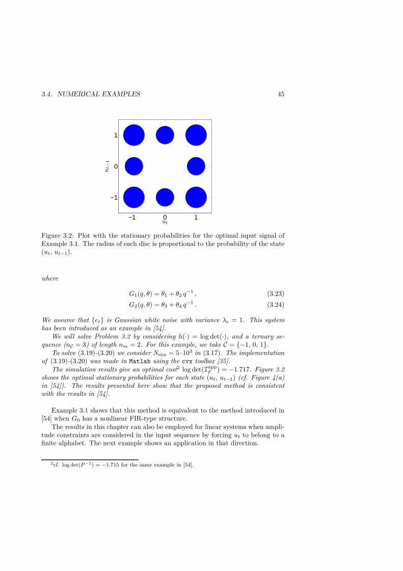
3.4. NUMERICAL EXAMPLES 45
−1 0 1
−1
0
1
ut
ut−
1
Figure 3.2: Plot with the stationary probabilities for the optimal input signal ofExample 3.1. The radius of each disc is proportional to the probability of the state(ut, ut−1).
where
G1(q, θ) = θ1 + θ2 q−1 , (3.23)
G2(q, θ) = θ3 + θ4 q−1 . (3.24)
We assume that et is Gaussian white noise with variance λe = 1. This systemhas been introduced as an example in [54].
We will solve Problem 3.2 by considering h(·) = log det(·), and a ternary se-quence (nC = 3) of length nm = 2. For this example, we take C = −1, 0, 1.
To solve (3.19)-(3.20) we consider Nsim = 5 ·103 in (3.17). The implementationof (3.19)-(3.20) was made in Matlab using the cvx toolbox [35].
The simulation results give an optimal cost2 log det(IappF ) = −1.717. Figure 3.2
shows the optimal stationary probabilities for each state (ut, ut−1) (cf. Figure 4(a)in [54]). The results presented here show that the proposed method is consistentwith the results in [54].
Example 3.1 shows that this method is equivalent to the method introduced in[54] when G0 has a nonlinear FIR-type structure.
The results in this chapter can also be employed for linear systems when ampli-tude constraints are considered in the input sequence by forcing ut to belong to afinite alphabet. The next example shows an application in that direction.
2cf. log det(P −1) = −1.715 for the same example in [54].

46 CHAPTER 3. INPUT DESIGN FOR NOE MODELS
Example 3.2 (Input design with amplitude constraints) In this example we con-sider the mass-spring-damper system introduced in [7]. The input, u, is the forceapplied to the mass and the output, y, is the mass position. The continuous-timesystem is described by the transfer function
G0(s) =1m
s2 + cm s+ k
m
, (3.25)
with m = 100 [Kg], k = 10 [N/m], and c = 6.3246 [Ns/m]. This choice results inthe natural frequency ωn = 0.3162 [rad/s] and damping ξ = 0.1. The noise etis white with zero mean and variance λe = 10−4. The system (3.25) is sampled byusing a zero-order-hold with sampling period Ts = 1 [s]. This gives the discrete-timesystem
G0(ut) =4.86 · 10−3 q−1 + 4.75 · 10−3q−2
1 − 1.84 q−1 + 0.94q−2ut . (3.26)
As a model, we define
G(ut; θ) =θ1 q
−1 + θ2q−2
1 + θ3 q−1 + θ4q−2ut , (3.27)
where
θ =[θ1 θ2 θ3 θ4
]⊤. (3.28)
We will solve Problem 3.2 for two cost functions: h(·) = − tr(·)−1 and h(·) =log det(·), subject to a binary sequence (nC = 2) of length nm = 2. In this example,we define C = −1, 1, and Nsim = 5 · 103.
The solution of Problem 3.2 for this example gives tr(IappF )−1 = 0.1108 and
log det(IappF ) = 28.22. Figure 3.3 and 3.4 present the stationary probabilities of
the optimal input signal for both cost functions. We can see that the stationaryprobabilities depend on the cost function h. However, both cost functions assignhigher stationary probabilities to the states (−1, −1) and (1, 1).
We can compare the performance of our approach with the method introducedin [7]. For this purpose, we generate an input sequence of length Nsim by runningthe Markov chain associated to the stationary distribution in Figure 3.3, and the4-states Markov chain presented in [7]. To guarantee that the input is a realizationof a stationary process, we discard the first 106 realizations of the Markov chain.The results for the sampled information matrix are trI−1
F = 1.8233 · 10−4 forthe 4-states Markov chain presented in [7], and trI−1
F = 1.6525 · 10−4 for ourmethod (we note that our results are consistent with those reported in [7], sincethe scaling factor Nsim is not considered here). Therefore, based on the variance ofthe parameter estimates, we conclude that the approach in this chapter gives betterresults for the example introduced in [7].
To have an idea of the computation time required for this example, the opti-mization was solved in a laptop Dell Latitude E6430, equipped with Intel Core i7

3.4. NUMERICAL EXAMPLES 47
−1 1
−1
1
ut
ut−
1
Figure 3.3: Plot with the stationary probabilities for the optimal input signal inExample 3.2 as in Figure 3.2. h(·) = − tr(·)−1.
−1 1
−1
1
ut
ut−
1
Figure 3.4: Plot with the stationary probabilities for the optimal input signal inExample 3.2 as in Figure 3.2. h(·) = log det(·).
2.6 [GHz] processor, and 8 [Gb] of RAM memory. The time required for the com-putation of elementary cycles to the computation of stationary probabilities is 1.9seconds.

48 CHAPTER 3. INPUT DESIGN FOR NOE MODELS
The results presented in the previous examples show that the method intro-duced in this chapter retrieves (or improves) the results in the literature. The nextexamples show an application of the input design method to a model structure notcovered by existing techniques.
Example 3.3 (Input design for nonlinear output-error models) Consider the blockdiagram depicted in Figure 3.1, where et is Gaussian white noise sequence withzero mean and variance λe = 1. The system is described by
G0(ut) =
xt+1 =1
θ01 + x2
t
+ ut ,
zt = θ02 x
2t ,
x1 = 0 ,
(3.29)
where θ0 =[θ0
1 θ02
]⊤=[0.8 2
]⊤. Notice that the system (3.29) cannot be de-
scribed as a Wiener-Hammerstein system, since the state equation is nonlinear inthe state xt.
To apply our method, we consider the model
G(ut; θ) =
xt+1 =1
θ1 + x2t
+ ut ,
zt = θ2 x2t ,
x1 = 0 ,
(3.30)
with θ =[θ1 θ2
]⊤= θ0.
We design an input of nseq = 104 samples as a realization of the pmf obtained bysolving Problem 3.2, with nm = 1, and C = −1, 0, 1. Problem 3.2 will be solvedfor h(·) = log det(·).
The stationary probabilities Pl obtained as the solution of Problem 3.2 arepresented in Figure 3.5. In this figure, we notice that the stationary probabilitiescannot be associated with samples obtained from a uniform distribution among thestates.
Given the stationary probabilities in Figure 3.5, we can use Algorithm 2.1 todesign a transition matrix to generate samples with the desired distribution. Theresulting transition matrix is given by
A =
0 0 00.47 0.47 0.470.53 0.53 0.53
, (3.31)

3.4. NUMERICAL EXAMPLES 49
(−1) (0) (1)0
0.2
0.4
0.6
Pl
Figure 3.5: Plot with the stationary probabilities for the optimal input signal inExample 3.3.
Table 3.1: Numerical results for the cost function in Example 3.3.
h(IF ) Graph Uniform Normal Binarylogdet(IF ) 3.67 2.77 3.12 3.47
where the rows and columns of A are indexed in the order (−1), (0), (1).
The second largest eigenvalue modulus (SLEM) for A defined in (3.31) is 0, andthe number of nonzero eigenvalues is 1, as expected by Theorem 2.3 in page 34.
Finally, we generate the input signal by running the Markov chain with tran-sition matrix (3.31) with random initial state in 0, 1, and recording the firstnseq = 104 samples. This is possible since the SLEM associated with the transitionprobability matrix (3.31) is zero, which implies that the chain will start in the sta-tionary distribution. To compare the result of the new method with those of standardinput signals, in Table 3.1 we present the results obtained for the cost function whenthe input is designed with the proposed method (logdet(IF ) = 3.67 in Graph),and when the input sequence is a realization of a sequence of independent and uni-formly distributed random variables with support [−1, 1] (logdet(IF ) = 2.77 inUniform). The results show that the proposed method for input design outperformsthe experiment result based on uniform samples. In addition, we can also compareour result with those obtained with the input being Gaussian distributed white noise,with zero mean and variance 1 (logdet(IF ) = 3.12 for Normal in Table 3.1), andwhen the input is a realization of a binary white noise process with values −1 and 1(logdet(IF ) = 3.47 for Binary in Table 3.1). In this case, the results obtained bythe Gaussian and the Binary distributed inputs are closer to the ones obtained bythe proposed input design method. However, our method still performs better thanthe input sequence based on random samples.
As an additional exercise, we can also compute the results obtained when theinput is designed for the following cases:
Case 1: nm = 2, C = −1, 0, 1 , (3.32)

50 CHAPTER 3. INPUT DESIGN FOR NOE MODELS
0.79 0.8 0.81
1.98
1.985
1.99
1.995
2
2.005
2.01
2.015
2.02
θ1
θ2
Figure 3.6: Plot with the 95 % confidence ellipsoids for input sequences of lengthnseq = 104, and the estimated parameters, Example 3.3. Blue, dashed line: Con-fidence ellipsoid for a binary input sequence (realizations marked with ∗). Red,continuous line: Confidence ellipsoid for the optimal input sequence, Case 2 (real-izations marked with circles).
Table 3.2: Numerical results for the cost function in Example 3.3, Cases 1-3.
h(IF ) Case 1 Case 2 Case 3logdet(IF ) 3.82 4.50 4.48
Case 2: nm = 1, C = −1, −1/3, 1/3, 1 , (3.33)
Case 3: nm = 1, C = −1, −0.5, 0, 0.5, 1 . (3.34)
Table 3.2 presents the results when the Markov chain associated with the Cases 1-3is employed to generate nseq = 104 samples. From these results we conclude thatwe can increase the information obtained from the input if we extend the memoryof the stationary process generating the input sequence. Moreover, the results aresignificantly better when we only extend the set C, which can be seen by comparingthe value of h of Case 1 with Cases 2 and 3 in Table 3.2. On the other hand, weobserve an interesting result in Table 3.2. In contrast to what we might expect,an increase of the magnitude of the elements in C does not necessarily imply anincrease of logdet(IF ). This phenomenon can be explained by the structure ofthe system (3.29), where we see that an increase in the amplitude of ut does notnecessarily imply that we obtain more information from the system. Since xt+1
depends on x−2t , then the future state will be small if the present state has a large

3.4. NUMERICAL EXAMPLES 51
value. Indeed, by comparing the value of h obtained in Case 2 and Case 3 inTable 3.2, we see that increasing the magnitude of the possible values for the inputdoes not imply an increase in the value of h.
To analyze the accuracy of the method, we present in Figure 3.6 the 95 % confi-dence ellipsoids for the input sequence generated from a random binary distribution,and from an optimal input obtained by solving Case 2. In addition, we also plot102 estimated parameters computed using the data set generated with both inputsequences. The results in the figure show that the proposed input design techniquedecreases the uncertainty region for the estimated parameters, compared to a randominput sequence of length nseq. This conclusion is also confirmed by the numericalestimates of θ0, which obey the distribution given by the theoretical bounds. There-fore, the proposed technique is an attractive alternative to increase the accuracy ofthe parameter estimates over the one obtained with random samples.
Example 3.4 (Input design for nonlinear output-error models revisited) Considerthe problem introduced in Example 3.3. As before, we will design an input of nseq =104 samples as a realization of the pmf obtained by solving Problem 3.2, for Case2 and Case 3 in Example 3.3. Problem 3.2 is solved for h(·) = − tr(·)−1.
Table 3.3: Numerical results for the cost function in Example 3.4.
h(IsF ) Case 2 Case 3 Unif. Normal Binary
− trIsF−1 −0.49 −0.45 −1.21 −0.96 −0.83
The results obtained by different input sequences of length nseq = 104 are pre-sented in Table 3.3, where Unif., Normal and Binary represent the results obtainedwith the random samples defined in Example 3.3. The results show that the pro-posed input design technique (Case 2 and Case 3 in Table 3.3) outperforms theinputs based on white noise samples.
To analyze the accuracy in this example, Figure 3.7 presents the 95 % confidenceellipsoids for the input sequence generated from a random binary distribution, andfrom an optimal input obtained by solving Case 3. In addition, we also plot 102
estimated parameters computed by using the data set generated with both inputsequences. In the same line as Figure 3.6, we see that the accuracy of the estimatedparameters is improved for the confidence sets, when we compare the optimal inputsequence with a white noise realization from a binary distribution. Therefore, themethod presented in this chapter is an effective approach to design input sequencesto identify the system (3.29).
Remark 3.5 The input design method presented in this chapter is close to thetechniques introduced in [18, 26]. In those approaches, the input is restricted to theset PC introduced in Chapter 2. However, the results in [18, 26] do not exploit the

52 CHAPTER 3. INPUT DESIGN FOR NOE MODELS
0.79 0.8 0.81
1.98
1.985
1.99
1.995
2
2.005
2.01
2.015
2.02
θ1
θ2
Figure 3.7: Plot with the 95 % confidence ellipsoids for input sequences of lengthnseq = 104, and the estimated parameters, Example 3.4. Blue, dashed line: Con-fidence ellipsoid for a binary input sequence (realizations marked with ∗). Red,continuous line: Confidence ellipsoid for the optimal input sequence, Case 2 (real-izations marked with circles).
connection between de Bruijn graphs and stationary processes, as it is presented inthis thesis, which allows to generate an input realization from an element in PC.
3.5 Conclusion
In this chapter, a new input design technique for identification of nonlinear output-error models has been described. The method considers the design of an inputsequence as a realization of a stationary process, which is obtained by maximizinga scalar cost function of the information matrix.
To obtain a computationally tractable problem, we parameterize the set of sta-tionary process in terms of convex combinations of the extreme points of the set.By assuming that the stationary process has finite memory and finite alphabet,the probability measures associated with the extreme points are computed as theset of prime cycles associated with the equivalent de Bruijn graph. Therefore, theinformation matrix associated with any element in the set of stationary processescan be computed as a convex combination of the information matrices obtained foreach extreme point. Due to the complexity of nonlinear model structures, the infor-mation matrices for each extreme point are obtained by numerical approximations.The main advantage of this approach is that the input design problem becomesconvex even for nonlinear model structures.

3.5. CONCLUSION 53
Finally, this chapter introduced numerical examples to illustrate the effective-ness of the proposed input design approach. The numerical examples show that theinput design method improves existing results in the literature. In addition, theproposed method can be employed to design input sequences to identify nonlinearmodel structures that are not covered by previous approaches.


Chapter 4
Optimal input design for nonlinear
state space models
In Chapter 3 a new method for input design for identification of nonlinear modelswas introduced. In that chapter, the discussion was restricted to nonlinear output-error models. The assumption on the model structure was introduced to simplifythe approximation of the Fisher information matrix, which is based on numericalapproximations. However, the method in Chapter 3 does not cover the case wherethe noise process also affects the internal states of the model. In these models, theapproximation of the Fisher information matrix given in Chapter 3 is no longervalid. Therefore, new approximation methods must be considered to extend theresults in Chapter 3 to more general nonlinear model structures.
In this chapter we provide an extension of the input design method introducedin Chapter 3 to nonlinear state space models. As in Chapter 3, we use a graphtheoretical approach to design an input sequence as a realization of a stationaryprocess, which maximizes a scalar cost function of the Fisher information matrix.To estimate the Fisher information matrices for the extreme points in the set ofstationary processes, we use particle methods to obtain the required estimations asthe sample covariance matrix of the score function. Then the optimization is solvedfor different realizations of the sample covariance matrix of the score function, andthe optimal pdf is obtained as the sample mean over the solutions obtained forthe different data realizations. Numerical examples show that the method is anattractive approach to design input sequences for identification of nonlinear statespace models.
55

56 CHAPTER 4. INPUT DESIGN FOR NONLINEAR SSM
4.1 Problem formulation
In this section1 we introduce an extension of the optimal input design formulationpresented in Chapter 3 to nonlinear state space models. The discussion in this partfollows the same lines as Section 3.1, with the difference that here we formulate theproblem to cover nonlinear state space models.
As in Chapter 3, the objective is to design an input signal u1:nseq = (u1, . . . , unseq),as a realization of a stationary process. This is done so that a state space model(SSM) can be identified with maximum accuracy as defined by a scalar function ofthe Fisher information matrix IF [59]. An SSM with states x0:T = (x0, . . . , xT ),inputs u1:T and measurements y1:T is given by
x0 ∼ µ(x0), (4.1a)
xt|xt−1 ∼ fθ(xt|xt−1, ut−1), (4.1b)
yt|xt ∼ gθ(yt|xt, ut). (4.1c)
Here, fθ(·) and gθ(·) denote known probability distributions parametrized by θ ∈Θ ⊂ Rnθ . In the sequel, we make the rather restrictive albeit standard assumptionthat there exists θ0 ∈ Θ such that the model (4.1) describes the system to beidentified when θ = θ0, i.e., there is no undermodeling. This assumption is necessaryin order to quantify the information retrieved from the experiment as a function ofthe Fisher information matrix.
We notice that we can write the joint distribution of states and measurementsfor (4.1) as
pθ(x1:T , y1:T |u1:T ) = µ(x0)
T∏
t=1
fθ(xt|xt−1, ut−1)gθ(yt|xt, ut). (4.2)
This quantity is used in the sequel for estimating IF by
IF = E
S(θ0)S⊤(θ0), (4.3a)
S(θ0) = ∇θ log pθ(y1:nseq)∣∣θ=θ0
, (4.3b)
where pθ(y1:nseq) and S(θ) denote the likelihood function and the score function,respectively. Note that the expected value in (4.3a) is with respect to the probabilitydistribution pθ(x0:T |y1:T ) and the realizations of u1:nseq .
We note that (4.3a) depends on the cumulative distribution function of u1:nseq ,Pu(u1:nseq). Therefore, the input design problem is to find a cdf P opt
u (u1:nseq)which maximizes a scalar function of (4.3a). We define this scalar function ash : Rnθ×nθ → R. To obtain the desired results, h must be a concave, nondecreas-ing, matrix function [5, pp. 108] (cf. Section 3.1). In this chapter we leave theselection of h to the user.
1Throughout this chapter we introduce a subindex in the cdfs and pdfs to emphasize therandom variables considered in the distribution.

4.2. A REVIEW ON SMC METHODS 57
Since P optu (u1:nseq) is assumed to describe a stationary Markov process with
memory nseq, the optimization must be constrained to the set
P = Pu : Rnseq → R|Pu(x) ≥ 0, ∀x ∈ Rnseq ;
Pu is monotone nondecreasing ;
limxi→∞
i=1, ..., nseqx=(x1, ..., xnseq )
Pu(x) = 1;
∫
v∈R
dPu ([v, z]) =
∫
v∈R
dPu ([z, v]) , ∀z ∈ Rnseq−1
. (4.4)
As in Chapter 3, here we restrict our problem to ut belonging to an alphabetwith finite cardinality nC . Thus, the set of pmfs associated with these processes is
PC = pu : Cnseq → R| pu(x) ≥ 0, ∀x ∈ Cnseq ;∑
x∈Cnseq
pu(x) = 1;
∑
v∈Cpu ([v, z]) =
∑
v∈Cpu ([z, v]) , ∀z ∈ C(nseq−1)
. (4.5)
Finally, the discussion in this section can be summarized as
Problem 4.1 Design an optimal input signal u1:nseq ∈ Cnseq as a realization frompoptu (u1:nseq), where
poptu := arg max
pu∈PC
h(IF (pu)) , (4.6)
with h : Rnθ×nθ → R a concave, nondecreasing, matrix function, and IF ∈ Rnθ×nθ
defined as in (4.3).
Before introducing the input design method, we review some material on sequentialMonte Carlo (SMC) methods.
4.2 A review on sequential Monte Carlo methods
SMC methods are a family of techniques that can be used, e.g., to estimate thefiltering and smoothing distributions in SSMs. Here we describe the idea behindSMC methods, and we introduce the required material to understand the estimationalgorithms employed in this chapter. The material in this section is based on[19, 22, 76].

58 CHAPTER 4. INPUT DESIGN FOR NONLINEAR SSM
SMC methods: main idea
The objective of SMC methods is to sample sequentially from target probabilitydensities p(x1:k)k≥1 of increasing dimension, where xk ∈ X , and each distributionp(x1:k) is defined on the product space X k. Writing
p(x1:k) =γk(x1:k)
Zk, (4.7)
it is only required that γk : X k → R+ is known pointwise; the normalizing constant
Zk =
∫
X k
γk(x1:k)dx1:k , (4.8)
might be unknown if γk is known pointwise. SMC provides an approximation ofp1(x1) and an estimate of Z1 at time 1, then an approximation of p2(x1:2), and anestimate of Z2 at time 2, and so on.
Monte Carlo methods
Consider initially approximating a generic probability distribution p(x1:T ) for some
fixed T . If we sample N independent random vectors x(i)1:T Ni=1 from p(x1:T ), then
the Monte Carlo method approximates functions of p(x1:T ) in the mean squaresense by using
p(x1:T ) =1
N
N∑
i=1
δ(x1:T − x
(i)1:T
), (4.9)
where δ(x) denoted the Dirac delta function located at x = 0. Based on thisapproximation, it is possible to approximate any marginal p(xk) by
p(xk) =1
N
N∑
i=1
δ(xk − x
(i)k
), (4.10)
and the expectation of any measurable function ϕT : X T → R, given by
E ϕT (x1:T ) =
∫
X T
ϕT (x1:T )p(x1:T ) dx1:T , (4.11)
is estimated as
EMC ϕT (x1:T ) :=
∫
X T
ϕT (x1:T )p(x1:T ) dx1:T =1
N
N∑
i=1
ϕT
(x
(i)1:T
). (4.12)
It is easy to check that (4.12) is an unbiased estimate of (4.11), and that its varianceis given by
Cov
EMC ϕT (x1:T )
=1
N
∫
X T
ϕ2T (x1:T )p(x1:T ) dx1:T − E ϕT (x1:T )
.
(4.13)

4.2. A REVIEW ON SMC METHODS 59
The main advantage of Monte Carlo methods over standard approximation tech-niques is that the variance of the approximation error decreases at a rate of O(1/N)regardless of the dimension of the space X T . However, there are at least two mainproblems with this idea:
(i) If p(x1:T ) is a complex high-dimensional probability distribution, then wecannot sample directly from it due to computational limitations.
(ii) Even if we knew how to sample exactly from p(x1:T ), the computational com-plexity of such a sampling scheme is typically at least linear in the number ofvariables T . Therefore, an algorithm sampling exactly from p(x1:T ), sequen-tially for each value of T , would have a computational complexity increasingat least linearly with T .
Importance sampling
In this part we address Problem (i) using the importance sampling (IS) method.IS relies on the introduction of an importance density pI(x1:T ) such that
p(x1:T ) > 0 ⇒ pI(x1:T ) > 0 ,
i.e., the distributions satisfy supp(pI) ⊆ supp(p). In this case, we have from (4.7)-(4.8) the following identities:
p(x1:T ) =wT (x1:T )pI(x1:T )
ZT, (4.14)
ZT =
∫
X T
wT (x1:T )pI(x1:T ) dx1:T , (4.15)
where wT (x1:T ) is the unnormalized weight function
wT (x1:T ) =γT (x1:T )
pI(x1:T ). (4.16)
In particular, we can select an importance density pI(x1:T ) from which it is easy todraw samples, e.g., the normal distribution, if this is consistent with the supportof p.
If we assume we draw N independent samples x(i)1:T Ni=1 from pI(x1:T ), then by
inserting the Monte Carlo approximation of pI(x1:T ) (the empirical distribution of
the samples x(i)1:T Ni=1) into (4.14)-(4.15), we have
p(x1:T ) =
N∑
i=1
w(i)T δ
(x1:T − x
(i)1:T
), (4.17)
ZT =1
N
N∑
i=1
wT
(x
(i)1:T
), (4.18)

60 CHAPTER 4. INPUT DESIGN FOR NONLINEAR SSM
where
w(i)T =
wT
(x
(i)1:T
)
∑Nj=1 wT
(x
(j)1:T
) , (4.19)
denotes the normalized weights.Based on the estimate (4.17), we can compute an estimate of (4.11) as
EIS ϕT (x1:T ) :=
∫
X T
ϕT (x1:T )p(x1:T ) dx1:T =
N∑
i=1
w(i)T ϕT
(x
(i)1:T
). (4.20)
Unlike the estimate EMC ϕT (x1:T ), the expression (4.20) is in general biased forfinite N . However, (4.20) is consistent in the number of samples N . The expressionfor the asymptotic bias is given by
limN→∞
N(
EIS ϕT (x1:T ) − E ϕT (x1:T ))
=
−∫
X T
p2(x1:T )
pI(x1:T )(ϕT (x1:T ) − E ϕT (x1:T )) d x1:T . (4.21)
Furthermore, EIS ϕT (x1:T ) satisfies
√N(
EIS ϕT (x1:T ) − E ϕT (x1:T ))
∈ As N (0, M) , (4.22)
where
M :=
∫
X T
p2(x1:T )
pI(x1:T )(ϕT (x1:T ) − E ϕT (x1:T ))
2d x1:T . (4.23)
As we can see from (4.21)-(4.23), both the bias and the variance for this methodare of order O(1/N).
The next sampling method addresses the issue related with the increasing com-putational complexity in the sample length T .
Sequential importance sampling
Sequential importance sampling (SIS) is a method that admits a fixed computa-tional complexity at each time step, and thus addresses Problem (ii). This methodconsiders an importance distribution which has the following structure:
pI(x1:T ) = pI(x1:T−1)pI(xT |x1:T−1)
= pI(x1)
T∏
t=2
pI(xt|x1:t−1) . (4.24)
From a practical perspective, Equation (4.24) means that to obtain particles x(i)1:T
distributed according to pI(x1:T ) at time T , we sample x(i)1 from pI(x1) at time 1,

4.2. A REVIEW ON SMC METHODS 61
then x(i)t is sampled from pI(xt|xi1:t−1) at time t, for t ∈ 2, . . . , T. The associated
unnormalized weights can be computed recursively using the decomposition
wT (x1:T ) =γT (x1:T )
pI(x1:T )
=γT−1(x1:T−1)
pI(x1:T−1)· γT (x1:T )
γT−1(x1:T−1)pI(xT |x1:T−1), (4.25)
which can be written in the form
wT (x1:T ) = wT−1(x1:T−1) · α(x1:T )
= w1(x1)T∏
k=2
α(x1:k) , (4.26)
where the incremental importance weight function α(x1:T ) is given by
α(x1:T ) :=γT (x1:T )
γT−1(x1:T−1)pI(xT |x1:T−1). (4.27)
The SIS method is summarized in Algorithm 4.1.Algorithm 4.1 provides the estimates p(x1:t) and Zt (equations (4.17)-(4.18)) of
p(x1:t) and Zt at any time t. In this framework, it seems that the only degree offreedom the user has at time t is the choice of pI(xt|x1:t−1) (the number of samplesN is also a degree of freedom, but it is fixed before executing the algorithm). Asensible strategy consists of selecting it so as to minimize the variance of wt(x1:t).This is achieved by selecting
poptI (xt|x1:t−1) = p(xt|x1:t−1) , (4.31)
as in this case the variance of wt(x1:t) conditional upon x1:t−1 is zero, and theassociated incremental weight is given by
αopt(x1:t) =γt(x1:t−1)
γt−1(x1:t−1)=
∫X γt(x1:t) dxt
γt−1(x1:t−1). (4.32)
We note that it is not always possible to sample from p(xt|x1:t−1), and nor isit always possible to compute αopt(x1:t). In these cases, we need to employ anapproximation of popt
I (xt|x1:t−1) for pI(xt|x1:t−1).In those scenarios in which the time required to sample from pI(xt|x1:t−1) and
to compute α(x1:t) is independent of t (which is the case if pI is chosen carefully andone is concerned with a problem such as filtering), it appears that SIS provides asolution for Problem (ii). However, the SIS method suffers from severe drawbacks.Even for standard IS, the variance of the resulting estimates increases exponentiallywith t [51]. A method to overcome this difficulty is presented in the next section.

62 CHAPTER 4. INPUT DESIGN FOR NONLINEAR SSM
Algorithm 4.1 Sequential importance sampling
Inputs: N (number of samples), pI(x1:T ) (importance distribution), and γT (x1:T ) (un-normalized pdf).
Output: x(i)1:T N
i=1 (realizations), and w(i)Ni=1 (normalized weights).
1: Sample x(i)1 from pI(x1) for i = 1 to N .
2: Compute the weights w1(x(i)1 ) = pI(x1), and
w(i)1 =
w1(x(i)1 )∑N
j=1w1(x
(i)1 )
, (4.28)
for i = 1 to N .3: for t = 2 to T do
4: Sample x(i)t from pI(xt|x
(i)1:t−1) for i = 1 to N .
5: Compute the weights
wt(x(i)1:t) = wt−1(x
(i)1:t−1) · α(x
(i)1:t) , (4.29)
where α given in (4.32), and
w(i)t =
wt(x(i)1:t)∑N
j=1wt(x
(i)1:t)
, (4.30)
for i = 1 to N .6: end for
Resampling
We have seen that IS (and therefore SIS) provides estimates whose variance in-creases with t. Resampling techniques are a key ingredient of SMC methods which(partially) solve this problem in some important scenarios.
Resampling is an intuitive idea with major practical and theoretical benefits.We consider first an IS approximation p(x1:T ) of the target distribution p(x1:T ).This approximation is based on weighted samples from pI(x1:T ), and does not pro-vide samples approximately distributed according to p(x1:T ). To obtain approxi-mate samples from p(x1:T ), we can simply draw samples from its IS approximation
p(x1:T ), where p(x1:T ) is defined in (4.17), with normalized weights w(i)T Ni=1. Then
we select x(i)1:T with probability w
(i)T . This operation is called resampling as it cor-
responds to sampling from an approximation p(x1:T ) which was itself obtained bysampling. If we are interested in obtaining N samples from p(x1:T ), then we canresample N times from p(x1:T ): This is equivalent to associating a number of off-
springs N(i)T with each sample x
(i)1:T in such a way that N
(1:N)T :=
(N
(1)T , . . . , N
(N)T
)
follow a multinomial distribution with parameter vector (N, w(1:N)T ), and associ-
ating a weight of 1/N with each offspring. Thus, we approximate p(x1:T ) by the

4.2. A REVIEW ON SMC METHODS 63
Algorithm 4.2 Systematic resampling
Inputs: x(i)1:T N
i=1 (realizations), and w(i)T N
i=1 (normalized weights).
Output: x(i)1:T N
i=1 (realizations), and N(i)T /NN
i=1 (resampled weights).
1: Sample U(1) from a uniform distribution defined on [0, 1/N ].2: Define U(i) := U(1) + (i − 1)/N for i ∈ 2, . . . , N.3: for i = 1 to N do
4: Set N(i)T =
∣∣∣
U(j) :∑i−1
k=1w
(k)T ≤ U(j) ≤
∑i
k=1w
(k)T
∣∣∣, where∑0
k=1µk := 0.
5: end for
resampled empirical measure
p(x1:T ) =N∑
i=1
N(i)T
Nδ(x1:T − x
(i)1:T
), (4.33)
where EN
(i)T
∣∣∣w(1:N)T
= Nw
(i)T . Hence p(x1:T ) is an unbiased approximation of
p(x1:T ).Many resampling schemes have been proposed in the literature [22]. One of
the most popular algorithms is systematic resampling, which is described in Algo-rithm 4.2. It can be shown that systematic resampling gives an unbiased estimateof the distribution p(x1:T ).
We clarify that resampling retrieves an estimate of E ϕT (x1:T ) with highervariance than the one obtained by using p(x1:T ). However, by resampling we removesamples with low weights with a high probability, which is useful when working withsequential techniques. If samples with low weights are preserved, then the approx-imation p(x1:T ) will lose accuracy as we increase the path length T . This problemis known as particle degeneracy, which is discussed in more detail in page 65.
Remark 4.1 The notion of offspring is not only important when talking aboutresampling, but it is also important for some of the particle methods discussed in
the next sections. For future reference, we introduce the ancestor index a(i)t . Given
a set of particles at time t, x(k)t Nk=1, we denote by a
(i)t the index of the particle
at time t − 1 from which x(i)t was generated. Figure 4.1 illustrates this idea. In
Figure 4.1, the directed edges between two nodes at different time instants expresswhich particles at time t− 1 generate which particles at time t.
Particle filterig
The name particle filter (PF) is a SMC method referring to the techniques em-ployed to obtain estimates of the sequence of target densities p(x1:t|y1:t)Tt=1 or itsmarginal p(xt|y1:t)Tt=1. Here we assume that the underlying process is describedfor all t ≥ 1 by equation (4.1).

64 CHAPTER 4. INPUT DESIGN FOR NONLINEAR SSM
.
.
.
xa
(2)t
t−1
xa
(1)t
t−1
xa
(N)t
t−1
x(N)t
x(2)t
x(1)t
.
.
.
Figure 4.1: Illustration of the ancestor index a(i)t .
The basic idea is to leverage SIS and resampling to propagate a collection of
N weighted random samples x(i)t , w
(i)t Ni=1 forward in time. These samples (com-
monly referred to as particles) constitute an empirical approximation that convergesasymptotically to the underlying target density p(xt|y1:t) as N → ∞.
The particle filter can be viewed as a framework to sequentially approximatethe filtering densities p(xt|y1:t)Tt=1. The resulting approximation is an empiricaldistribution of the form
p(xt|y1:t) =
N∑
i=1
w(i)t δ(xt − x
(i)t ) . (4.34)
Intuitively speaking, each particle x(i)t can be understood as a possible state of the
underlying system, where the corresponding weight w(i)t contains information about
how probable that particular state is.In this subsection we introduce the method that will prove to be useful for the
results presented in this chapter: the auxiliary particle filter (APF).
The auxiliary particle filter
The auxiliary particle filter (APF) [70] is a method which can be used to include theinformation available in the current observation yt not only for proposing the newstate xt (as it is done in the PF method2), but also when proposing the ancestorindex at (recall that at is the ancestor index of the particles at time t). Thus, weincrease the probability of resampling particles at time t − 1 that agree with thecurrent observation yt when compared with the PF approach.
2We refer to [22, 76] for more details of the particle filter algorithm.

4.2. A REVIEW ON SMC METHODS 65
To continue, we define a function ν : X × Y → R, such that for each particle i,i ∈ 1, . . . , N we compute the factors
ν(i)t−1 := ν(x
(i)t−1, yt) , (4.35)
referred to as adjustment multipliers. The adjustment multipliers are user definedfunctions, which are employed to adjust the empirical distributions to sample andpropagate the particles. We note that (4.35) depends only on the previous particlesand on the current observation, which are available in the resampling step at timet. The adjustment multipliers are then used to define a proposal distribution forthe ancestor index at according to
P
at = i
∣∣∣∣x
(j)t−1, w
(j)t−1
Nj=1
=
w(i)t−1ν
(i)t−1∑N
l=1 w(l)t−1ν
(l)t−1
. (4.36)
Once the ancestor indices are generated, we propagate the particles to time t by
simulating x(i)t ∼ pprop(xt|x(i)
t−1, yt) for i ∈ 1, . . . , N, where pprop(xt|xt−1, yt) is
the proposal distribution, and x(i)t−1 = x
(at)t−1 .
In addition to the elements introduced in this part, the APF needs the definition
of a weight function from which w(i)t are generated. For the APF, the weight
function w : X 2 × Y → R is defined as3
w(xt−1, xt, yt) =g(yt|xt) f(xt|xt−1)
ν(xt−1, yt) pprop(xt|xt−1, yt). (4.37)
Algorithm 4.3 summarizes the auxiliary particle filter method. We notice that, attime t, the APF performs three steps: (i) resampling of the particles at time t− 1,(ii) propagation of the particles from time t − 1 to time t, and (iii) normalizedweighting of the set of particles at time t. These steps are a common framework ofparticle filter methods [76].
Particle degeneracy
In principle, the SMC can be used to obtain an approximation of a sequence ofdensities p(x1:t|y1:t)t≥1 of growing dimension, where the approximations tends tothe true distributions asymptotically in the number of particles N , i.e., as N → ∞.However, the task of approximating p(x1:t|y1:t)t≥1 is inherently impossible tosolve using a finite number of particles N . To illustrate this, assume that weemploy a particle filter to target the joint smooth density p(x1:t|y1:t). At time
s we generate N unique4 particles x(i)s Ni=1 from the proposal density, and we
append these to the existing particle trajectories x(i)1:s−1Ni=1. Therefore, we have a
3We note that the PF is obtained from the APF when ν(xt−1, yt) = 1 [76].4By unique we mean that each particle x
(i)s is a different realization from the proposal density,
for i ∈ 1, . . . , N.

66 CHAPTER 4. INPUT DESIGN FOR NONLINEAR SSM
Algorithm 4.3 Auxiliary particle filter (APF)
1: Initialization (t = 1):
2: Sample x(i)1 ∼ pprop(x1|y1).
3: Compute the importance weights w(i)1 = g(y1|x(i)
1 )µ(x(i)1 )/pprop(x
(i)1 |y1), and
normalize w(i)1 = w
(i)1 /
∑Nj=1 w
(j)1 .
4: for t = 2 to T do5: Compute the adjustment multipliers ν
(i)t−1 = ν(x
(i)t−1, yt).
6: Resampling: Resample x(i)t−1Ni=1 with probabilities proportional to
w(i)t−1ν
(i)t−1Ni=1 to generate the equally weighted particle system x(i)
t−1, 1/NNi=1.
7: Propagation: Sample x(i)t ∼ pprop(xt|x(i)
t−1, yt).
8: Weighting: Compute w(i)t = w(x
(i)t−1, x
(i)t , yt) and normalize:
w(i)t =
w(i)t∑N
j=1 w(j)t
.
9: end for
weighted particle system x(i)1:s, w
(i)s Ni=1 approximating the joint smoothing density
at time s. If we assume that the particle trajectories are resampled, then we obtain
the particle system x(i)1:s, 1/NNi=1. We recall that the purpose of resampling is
to remove particles with small weights, and duplicate particles with large weights.Thus, the resampling step has the effect of reducing the number of unique particles.In consequence, over time each consecutive resampling of the particle trajectorieswill reduce the number of unique particles at time s. Eventually the particle systemat time s will collapse into a single trajectory. This problem is referred to as particledegeneracy. In other words, the resampling step inevitable results in that for anytime s there exists t > s such that the PF approximation p(x1:t|y1:t) consists of asingle particle at time s.
A relevant question is to consider if it is possible (at least partly) to “undo” theparticle degeneracy. One idea is to investigate if it is possible to initiate a backwardssweep starting from the particle filter representation of p(xt|y1:t), and reintroducediversity among the particles by some form of backwards computation. This ques-tion5 is addressed by a family of algorithms referred to as particle smoothers, whichare introduced in the next subsection.
5Other solutions to the particle degeneracy problem involves increasing the number of particlesN , or the fully-adapted PF [76].

4.3. NEW INPUT DESIGN METHOD 67
Particle smoothing
As previously mentioned, if we only use the particle filter to compute the sequenceof densities p(x1:t|y1:t)t≥1, then the approximations p(x1:t|y1:t)t≥1 will have theparticle degeneracy problem. To overcome this issue, we employ particle smoothersto compute the joint distribution. In this subsection, we introduce the fixed-lagsmoother.
The fixed-lag smoother
The fixed-lag (FL) smoother [50] is an algorithm employed to estimate the smooth-ing densities, which decreases the particle degeneracy problem experienced withthe particle filter. The fixed-lag smoother is used to approximate functionals inadditive form. This means that, provided F : X T → R is a functional dependent onx1:T , we can use the fixed-lag smoother to approximate expected values dependenton F if and only if F can be written as
F(x1:T ) =
T−1∑
t=1
st(xt:t+1) , (4.38)
where stt≥1 is a sequence of measurable functions (which may depend on theobserved data y1:T ) [68].
The key assumption in the fixed-lag smoother is that the pdf pθ(xt|y1:T ) canbe approximated by pθ(xt|y1:κt
), for κt = min(t + ∆, T ) with some fixed-lag ∆,0 ≤ ∆ ≤ T . Therefore, the fixed-lag smoother assumes that the mixing propertiesof the process (4.1) are such that all the measurements ykk>∆ have a negligibleeffect on the conditional pdf of xt given y1:T , denoted by p(xt|y1:T ).
The FL smoother employs the same algorithm as the APF (presented in Algo-rithm 4.3). However, the FL smoother approximates the two-step filtering distri-bution by
p (xt−1:t) =
T−1∑
t=1
N∑
i=1
w(i)κtδ
(xt−1:t − (x
a(i)κt,t
t−1 , xa
(i)κt,t−1
t )
), (4.39)
where a(i)κt,t denotes the particle at time t which is the ancestor of particle i at time
κt.It can be shown that, under some strict mixing assumptions, the variance and
the bias of the FL smoother are of order O(T logT /√N) and O(T logT /N)
respectively. We refer to [68] for more details.
4.3 New input design method
In this section we will introduce a new input design method for nonlinear statespace models.
68 CHAPTER 4. INPUT DESIGN FOR NONLINEAR SSM
Graph theoretical input design
Problem 4.1 will be solved using the graph theoretical approach presented in Chap-ter 3. To this end, we will consider u1:nseq as a realization of a Markov processwith memory nm, where nm < nseq. Thus, we obtain a tractable description of thepolytope PC in term of its extreme points. Following the notation introduced inChapter 2, we will refer to VPC
= v1, . . . , vnV as the set of the extreme points of
PC .To find all the elements in VPC
, we will make use of the results introduced inSection 2.2 in page 23. Indeed, we know that the set VPC
can be described in termsof the set of prime cycles in the equivalent de Bruijn graph GCnm (cf. Figure 2.1in page 23). Moreover, the set of prime cycles in GCnm can be computed fromthe set of elementary cycles in GCnm−1 (Lemma 2.2 in page 29). Finally, by usingTheorem 2.1 in page 28, we have that the probability measures associated with theelements in VPC
are known once the set of prime cycles in GCnm is obtained.Since we know the prime cycles in GCnm , it is possible to generate an input
sequence ujtTt=0 from vj , which will be referred to as the basis inputs. We referto Example 2.4 in page 30 for an illustration on how to obtain an input sequencefrom a given prime cycle.
Given ujtTt=0, we can use it to obtain the corresponding information matrix
for vj ∈ VPC, say I(j)
F . However, in general the matrix I(j)F cannot be computed
explicitly. To overcome this problem, we use SMC methods to approximate I(j)F ,
as discussed in the next subsection.
Estimation of the score function
Consider (4.3). If samples of the score function were available we could approximatethe Fisher information matrix (4.3) as the sample covariance matrix of the scorefunction. However, the samples of the score function are not available. Therefore,we need to compute estimates associated with the score function. To this end, wewill use SMC methods to estimate the score function, in particular we will use ideasfrom particle filter and fixed-lag particle smoothers.
As discussed in Section 4.2, the particle system is sequentially computed usingtwo steps: (i) sampling/propagation and (ii) weighting. The first step can be seenas sampling from a proposal kernel,
a(i)t , x
(i)t ∼ wat
t−1∑Nk=1 w
(k)t−1
Rθ,t(xt|xat
t−1, ut−1), (4.40)
where we append the sampled particle to the trajectory by x(i)1:t = x(i)
1:t−1, x(i)t .
Here, Rθ,t(·) denotes the propagation kernel6 and the ancestor index a(i)t denotes
6For the purpose of this subsection, the propagation kernel can be seen as the productν(xt−1, yt) pprop(xt|xt−1, yt) in equation (4.37).

4.3. NEW INPUT DESIGN METHOD 69
the index of the ancestor at time t − 1 of particle x(i)t . In the second step, we
calculate the (unnormalized) importance weights,
w(i)t ,
gθ(yt|x(i)t , ut)fθ(xt|x(i)
t−1, ut−1)
Rθ,t(xt|x(i)t−1, ut−1)
. (4.41)
We make use of Fisher’s identity7 [8, 25] to rewrite the score function (4.3b)into a form that can be used in combination with SMC methods. This results inthat we can write
∇θ log pθ(y1:T |u1:T ) = E
∇θ log pθ(x1:T , y1:T |u1:T )∣∣y1:T , u1:T
. (4.42)
By using (4.2) into (4.42), and writing out the expected value, we obtain
∇θ log pθ(y1:T |u1:T ) =
T∑
t=1
∫
X 2
ξθ(xt−1:t, ut)pθ(xt−1:t|y1:T ) dxt−1:t, (4.43)
with
ξθ(xt−1:t, ut) = ∇θ
[log fθ(xt|xt−1, ut−1) + log gθ(yt|xt, ut)
],
which depends on the two-step marginal smoothing densities. We notice that thesum in (4.43) appears since the logarithm function transforms the product (4.2)into a sum. The APF can be used to estimate these quantities but this leads topoor estimates with high variance, due to problems with particle degeneracy.
Instead, we use an FL-smoother to estimate the smoothing densities, whichreduces the variance of the score estimates [68]. We refer to [16] for more detailsabout the FL-smoother and its use for score estimation. Based on the estimatesfor the target distributions obtained from Algorithm 4.3, the estimate of the scorefunction is given by
S(θ) :=T∑
t=1
N∑
i=1
w(i)κtξθ
(xa
(i)κt,t
t , xa
(i)
κt,t−1
t−1 , ut
), (4.44)
where a(i)κt,t denotes the particle at time t which is the ancestor of particle i at time
κt.In the SMC literature, the Fisher information matrix is often estimated by
the use of Louis’ identity8 [8, 62]. However, this approach does not guaranteethat the information matrix estimate is positive semidefinite. Based on numericalexperience, this standard approach also leads to poor accuracy.
Instead, we make use of the fact that the information matrix can be expressedas (4.3), i.e., the covariance matrix of the score function. Hence, a straightforward
7We refer the reader to Appendix C for a derivation of the Fisher’s identity.8We refer the reader to Appendix C for a derivation of Louis’ identity.

70 CHAPTER 4. INPUT DESIGN FOR NONLINEAR SSM
method for estimating the information matrix is to use the Monte Carlo covariance
estimator over some realizations of the system, given by y(m)1:T Mm=1. If we denote
each Monte Carlo estimate of the score function by Sm(θ), the information matrixcan be estimated using
IF =1
M − 1
M∑
m=1
Sm(θ)S⊤m(θ), (4.45)
where M denotes the number of score estimates. Note that this is an estimate of theFisher information matrix as the Monte Carlo estimator averages over the systemrealizations. The estimate is positive semidefinite by construction but inherits somebias from the FL-smoother, see [68] for more information. This problem can behandled by using a more computationally costly particle smoother. In Section 4.4we present results indicating that this bias does not affect the resulting input signalto any large extent.
Solution to the optimization problem
As in Chapter 3, we associate I(j)F nV
j=1 with the elements in VPC, the set of extreme
points of PC. By defining α := α1, . . . , αnV ∈ RnV , we introduce Iapp
F (α) as theinformation matrix associated with one element in PC for a given α such thatαj ≥ 0, j ∈ 1, . . . , nV,
∑nV
j=1 αj = 1. Therefore, finding the optimal IappF (α) is
equivalent to determining the optimal weighting vector α.Hence, we can rewrite Problem 4.1 as
αopt = arg maxα∈R
nV
h(IappF (α)) , (4.46a)
s.t. IappF (α) =
nV∑
j=1
αj I(j)F , (4.46b)
nV∑
j=1
αj = 1 , (4.46c)
αj ≥ 0 , for all j ∈ 1, . . . , nV , (4.46d)
To solve the optimization problem (4.46), we need to estimate the informationmatrix for each basis input.
The information matrix estimate in (4.45) can be used to estimate the Fisherinformation matrix for each basis input. A simple solution is therefore to plug-in theestimates and solve the convex optimization problem (4.46) using some standardsolver. However, by doing this we neglect the stochastic nature of the estimatesand disregard the uncertainty. In practice, this leads to bad estimates of α.
Instead, we propose the use of a Monte Carlo method which involves two dif-ferent steps over K iterations. In step (a), we compute the information matrix

4.4. NUMERICAL EXAMPLES 71
Algorithm 4.4 Optimal input design using SMC methods
Inputs: Algorithm 4.3, K (no. MC runs) and M (size of each batch).Output: α⋆ (estimate of the optimal weighting of the basis inputs).
1: for k = 1 to K do
2: Generate M samples using Algorithm 4.3 for each basis input.3: Estimate the information matrix by (4.45) for each basis input.4: Solve the problem in (4.46).5: Set α(k) as the weighting factors obtained from the solver.6: end for
7: Compute the sample mean of α = α(1), . . . , α(K), denote it as α⋆.
estimates I(j)F for each input using (4.45). In step (b), we solve the optimization
problem in (4.46) using the estimates I(j)F nV
j=1 to obtain the optimal weights α(k)
at iteration k. The estimate of the optimal weighting vector α⋆ is computed as thesample mean of α = α(1), . . . , α(K), which can be complemented with a confidenceinterval. The outline of the complete procedure is presented in Algorithm 4.4.
Summary of the method
The proposed method for designing input signals in Cnm considers the approachpresented in Chapter 3, page 43, with the difference that the approximation ofthe Fisher information matrix in step 4 is performed using Algorithm 4.3, and theoptimization is solved using Algorithm 4.4.
4.4 Numerical examples
The following examples present some applications of the proposed input designmethod.
Example 4.1 Consider the linear Gaussian state space (LGSS) system with pa-
rameters θ =[θ1 θ2
]⊤,
xt+1 = θ1xt + ut + vt, vt ∼ N (0, θ22),
yt = xt + et, et ∼ N (0, 0.12),
where the true parameters are θ0 =[0.5 0.1
]⊤. We design experiments to iden-
tify θ with nseq = 5 · 103 time steps, memory length nm = 2, and an input as-suming values C = −1, 0, 1. The optimal experiments maximize h(Iapp
F (α)) =log det(Iapp
F (α)), and h(IappF (α)) = − tr
(IappF (α))−1
.
We generate ujtTt=0 for each vj ∈ VPC, j ∈ 1, . . . , 8 (T = 102) to compute the
approximation (4.45) for each I(j)F . Finally, the optimal input u1:nseq is computed
by running a Markov chain with poptu (u1:nm
) as stationary pmf, where we discard

72 CHAPTER 4. INPUT DESIGN FOR NONLINEAR SSM
Table 4.1: h(IF ), Example 4.1.
Input / h(IF ) log det(IF ) − tr
(IF )−1
Optimal (log det) 20.67(0.01) −1.51 · 10−4(5.18 · 10−7)Optimal (tr) 20.82(0.01) −1.32 · 10−4(4.45 · 10−7)
Binary 20.91(0.01) −1.21 · 10−4(4.51 · 10−7)Uniform 19.38(0.01) −5.32 · 10−4(2.12 · 10−6)
the first 2 · 106 samples and keep the last nseq = 5 · 103 ones. In addition, weconsider K = 100, M = 5 · 103 and N = 103. As a benchmark, we generate nseq
input samples from uniformly distributed white noise with support [−1, 1], and thesame amount of samples from binary white noise with values −1, 1. These inputsamples are employed to compute an approximation of IF via (4.45).
Table 4.1 condenses the results obtained for each input sequence, where Optimal(log det) and Optimal (tr) represent the results for the input sequences obtainedfrom optimizing log det(Iapp
F (α)), and − tr
(IappF (α))−1
, respectively. The 95%
confidence intervals are given as ± the value in the parentheses. From the datawe conclude that, for this particular example, the binary white noise seems to bethe best input sequence. Indeed, the proposed input design method tries to mimicthe binary white noise excitation, which is clear from the numbers in Table 4.1.In this example, the results obtained with the proposed input design technique aredegraded due to the variability in the optimization problem, which can be reducedby increasing the number of particles N in the estimation of the score function, byincreasing the number of realizations M for the score function, and by increasingthe number of iterations K.
Example 4.2 In this example we consider the system in [34, Section 6], given by
xt+1 = θ1xt +xt
θ2 + x2t
+ ut + vt, vt ∼ N (0, 0.12),
yt =1
2xt +
2
5x2t + et, et ∼ N (0, 0.12),
where θ =[θ1 θ2
]⊤denotes the parameters with true values θ0 =
[0.7 0.6
]⊤. We
design an experiment with the same settings as in Example 4.1 maximizing
h(IappF (α)) = log det(Iapp
F (α)) .
A typical input realization obtained from the proposed input design method is pre-sented in Figure 4.2.
Table 4.2 presents the results obtained for each input sequence, where Optimalrepresents the result for the input sequence obtained from optimizing log det(Iapp
F (α)).The 95% confidence intervals are given as ± the value in the parentheses. Fromthese data we conclude that the extended input design method improves the experi-ment results obtained for binary and uniformly distributed samples.

4.5. CONCLUSION 73
0 20 40 60 80 100−1.5
−1
−0.5
0
0.5
1
1.5
t
ut
Figure 4.2: Input realization, Example 4.2.
Table 4.2: h(IF ), Example 4.2.
Input / h(IF ) log det(IF )Optimal 25.34(0.01)Binary 24.75(0.01)
Uniform 24.38(0.01)
4.5 Conclusion
In this chapter we discussed an extension of the input design method considered inChapter 3. The extension considers a more general model structure in the form of anonlinear state space description. Based on the approach introduced in Chapter 3,we design the input sequence by maximizing a scalar cost function of the Fisherinformation matrix over the set of stationary processes with finite memory andfinite alphabet.
The main difficulty in this chapter is associated with the computation of theFisher information matrix for the set of basis inputs. Since we assume a moregeneral nonlinear model structure, the Monte Carlo approximation described inChapter 3 cannot be employed here. To overcome this issue, we use particle methodsto approximate the Fisher information matrices for the set of basis inputs. Sincethe method is based on numerical approximations, the resulting optimization isperformed several times over different realizations, and the final result is the samplemean over the different realizations. Numerical examples show that the proposedtechnique can be employed for designing input sequences to identify nonlinear statespace models.
As it might be expected, the computational complexity of this approach is notonly related to the computation of the basis inputs, but it is also connected withthe number of particles and the length of the input employed to estimate the scorefunction. Future work in this subject will be related with the reduction of thecomputational complexity associated with the estimation of the score function.


Part II
Applications
75


Chapter 5
Input design for systems with
quantized data
In this chapter, we present one application of the proposed input design method toidentify systems subject to quantized measurements. This problem is of relevancebecause of the many applications where quantized measurements are used. For ex-ample, quantized measurements are widely used in networked control and wirelesscommunications, due to the noise immunity of digital communication channels. Infact, due to constraints on the communication channels, such as noise and limitedbandwidth, it is impossible to transmit data with infinite precision. Thus, quan-tization is an effective way to reduce use of the transmission resource, and meetthe bandwidth constraint of a communication channel. However, quantization is alossy compression method, hence the validity or performance of parameter identi-fication may be affected by quantization. This could also result in the deterioratedperformance of adaptive control techniques.
In wireless communications, for example, quantized system identification is cru-cial for echo cancellation and blind communication channel estimation, see [31] andthe references therein. This means that quantized system identification is very im-portant as the use of wireless technologies is now extensive in many areas of society,and it is expected to increase.
A particular type of quantized system is where the quantizer can take only 2 pos-sible values (binary signals). This kind of configuration has attracted considerableattention [13, 48, 56]. In fact, binary-valued (or quantized) sensors are commonlyused in practical systems. They are exemplified by switching sensors for exhaustgas oxygen, photoelectric sensors for position, Hall-effect sensors for speed and ac-celeration, gas content sensors in the gas and oil industry, and distributed one-bitwireless sensors [63, 71, 99]. In particular, for any remotely controlled system, sig-nal quantization is mandatory. Compared to regular sensors, binary-valued sensorsare usually far more cost effective. However, they provide very limited informationon the process.
77

78 CHAPTER 5. INPUT DESIGN FOR QUANTIZED SYSTEMS
FIRxt Qut
wt
yt
Figure 5.1: FIR system with quantized output.
The problem of input design for quantized systems has been treated in previousworks [10, 11, 12, 98]. In [98] conditions under which consistent estimates can beobtained are presented. In particular, [98] recommends the use of periodic signals.Even though periodic inputs have shown to asymptotically achieve the Cramér-Raolower bound (CRLB), their use may be inadequate for tracking control applications,since the output will not follow the desired trajectory [65].
In [12], the input design problem is carried out within a worst case framework,based on the set membership paradigm of uncertainty representation. There, theauthors assume uncertainty in the parameters, and extend the previous work [11]from binary sensors to multilevel sensor thresholds.
The work [65] asserts that the input assuring strong consistency of the estimatesis a persistently exciting signal of certain order r, as long as the quantizer is optimalin the sense of minimizing the error between the measurement and the input to thequantizer. However, the design of this signal is not carried out.
To use the input design technique proposed in previous chapters for identifica-tion of model structures with quantized output, we need an estimate of the Fisherinformation matrix (FIM) obtained when using the set of basis inputs. In thischapter an estimate of the FIM is given, based on the so-called Fisher’s identity(cf. Subsection C.2 [66]). A numerical example shows that the proposed techniqueis suitable for solving the input design problem for identification of models withquantized outputs.
5.1 Input design problem
We focus on the problem of input design for quantized output systems. In partic-ular, we have a system as in Figure 5.1, where noise enters between the linear FIRsystem and the quantizer. The noise, wt, is assumed to be zero-mean Gaussianwith variance σ2. We also assume that σ2 is known.
Remark 5.1 Note that the assumption about the noise variance being known isonly necessary for the experiment design, and not for the estimation problem. Asshown in [31], the noise variance can also be estimated.
5.1. INPUT DESIGN PROBLEM 79
The system can be described by
xt = ϕ⊤t θ0 + wt, wt ∼ N (0, σ2)
yt = Q[xt],(5.1)
where xt is a scalar, the parameter vector θ0 is of dimension nθ, ϕt is a vector ofdimension nθ, and σ2 ∈ R is the noise variance. Q : R → V represents a quantizer,which is a map from R the set of a scalars to the finite set V = v1, v2, · · · , vM ofreal numbers, i.e.,
Q[x] =
v1, if x ∈ Ω1,...
vM , if x ∈ ΩM ,
(5.2)
where Ωi, i ∈ 1, . . . ,M conform a partition of R.Since the system is described by (5.3), we consider the model set
M =
xt = ϕ⊤
t θ + wt, wt ∼ N (0, σ2)
yt = Q[xt],
∣∣∣∣∣ θ ∈ Θ
. (5.3)
The problem of interest is to design the input u1:nseq = (u1, u2, . . . , unseq)such that the parameter θ0 is better estimated compared to any other input signal.From (5.1) we see that the output yt contains information about the parameter θ0.Moreover, the information available in yt depends on the vector ϕt, which dependson the input ut. Therefore, the input sequence u1:nseq can be designed to maximizethe information about θ0 available in yt.
To formulate the input design problem, consider the FIM (recall Lemma 1.1 inpage 9)
IeF = E
∂lθ(y1:nseq)
∂θ
∣∣∣∣θ=θ0
∂lθ(y1:nseq)
∂θ⊤
∣∣∣∣θ=θ0
∈ Rnθ×nθ , (5.4)
wherelθ(y1:nseq) = log pθ(y1:nseq) (5.5)
is the log-likelihood function, with pθ(y1:nseq) being the probability distribution ofthe data, y1:nseq , given the parameter θ. The FIM defines the maximal accuracythat an unbiased estimator of θ0 can achieve, due to the Cramér-Rao bound (cf.Lemma 1.1 in page 9):
Cov(θ) IeF −1, (5.6)
where θ denotes the estimator of θ0.Given a concave matrix non-decreasing function h : Snθ
+ → R, where Snθ
+ corre-sponds to the space of symmetric and positive-semidefinite matrices of dimensionnθ × nθ, an input design problem can be posed as

80 CHAPTER 5. INPUT DESIGN FOR QUANTIZED SYSTEMS
Problem 5.1 Design an input sequence uopt1:nseq
for the quantized system (5.1) suchthat
uopt1:nseq
= arg maxu1:nseq
h(IeF )
s. t. |ut| ≤ umax, for all t ∈ 1, . . . , nseq ,(5.7)
where umax > 0 is a prescribed upper bound on the input amplitude.
Problem 5.1 is difficult to solve. The main issue is that the optimization of h(IeF )as a function of u1:nseq is typically non-convex, which gives place to numerical diffi-culties (e.g., local optima and initialization). However, if we relax the requirementson u1:nseq to be a realization of a stochastic process with memory nm ≤ nseq andfinite alphabet C, then we can use the method described in Chapter 3 to solve asuboptimal approximation of Problem 5.1. By a suitable definition of C, the con-straint in the input design problem can be implicitly considered. However, to usethe results in Chapter 3, we need an expression for IF to compute by numericalsimulations the required matrices to set up the optimization. The next sections arefocused on providing such expression for IF when the system is described accordingto Equation (5.1).
5.2 Background on maximum likelihood estimation with
quantized output data
The maximum likelihood (ML) estimation problem can be posed as:
θnseq = arg maxθlθ(y1:nseq), (5.8)
where the log-likelihood function lθ(y1:nseq) is given by (5.5). For the problem ofinterest in this chapter, we can write (5.5) as
lθ(y1:nseq) =
nseq∑
t=1
lt(θ), lt(θ) = log pθ(yt|y1:t−1). (5.9)
Assumption 5.1 The input u1:nseq = utnseq
t=1 is an exogenous signal, and the FIRsystem is in open loop.
Remark 5.2 Notice that the system (of interest) is FIR, thus,
lt(θ) = log pθ(yt|y1:t−1) = log pθ(yt) .
Before introducing the next assumption, we need the following definitions [59]:

5.2. BACKGROUND ON ML ESTIMATION 81
Definition 5.1 (Uniformly stable filters) Consider the family of filters
H = Gβ(q) =∞∑
k=1
gβ, kq−k |β ∈ B . (5.10)
The family of filters H is uniformly stable if and only if
|gβ, k| ≤ gk, for all β ∈ B , (5.11)
where gk∞k=1 satisfies
∞∑
k=1
gk < ∞ . (5.12)
Definition 5.2 (Quasi-stationary signal) A signal st is said to be quasi-stationaryif and only if, for all integers t, r, and τ ,
Est = ms(t) , (5.13)
Est sr = Rs(t, r) , (5.14)
limnseq→∞
1
nseq
nseq∑
i=1
Rs(i, i− τ) = R′s(τ) , (5.15)
where the functions ms, Rs, satisfy |ms(t)| ≤ C, |Rs(t, r)| ≤ C, for some finiteC ≥ 0.
Definition 5.3 (Informative enough data sets) A quasi-stationary data set yt, utis informative enough with respect to the model set M if and only if, for twooptimal one-step ahead prediction filters W1(q) and W2(q), derived from any twomodels in the model set M, the expression
limnseq→∞
1
nseq
nseq∑
t=1
E[(W1(q) −W2(q)) zt]2 = 0 , (5.16)
implies that W1(eiω) = W2(eiω) for almost all ω, where zt :=[y⊤t u⊤
t
]⊤.
Assumption 5.2 The vector of parameters θ, the input ut and the noise wt satisfythe following regularity conditions [59, Theorem 8.3]:
• The data set yt, ut is such that for some filters d(i)t, k,
xt =
∞∑
k=1
d(1)t, kut−k +
∞∑
k=1
d(2)t, kwt−k,
yt = Q[xt].
(5.17)

82 CHAPTER 5. INPUT DESIGN FOR QUANTIZED SYSTEMS
• ut is a bounded, external input sequence.
• wt is a sequence of independent random variables with zero mean values,and bounded moments of order 4 + δ for some δ > 0.
• The family of filters d(i)t, k∞
k=1, i ∈ 1, 2, t ≥ 1 is uniformly stable.
• The signals yt, ut are jointly quasi-stationary.
• There exists a θ0, such that yt is described by (5.1) when θ = θ0 (no under-modeling).
• The data set yt, ut is informative enough with respect to the model structure(5.1).
The conditions presented in Assumption 5.2 guarantee that the solution θnseq of theoptimization problem in (5.8) converges (in probability or a.s.) to the true solutionθ0 as nseq → ∞ [58].
The maximum likelihood estimation (5.8) requires the computation of the log-likelihood function associated to a model in the set (5.3), which is difficult to handledue to the quantizer in (5.1). To overcome this issue, we use the expectation max-imization (EM) algorithm to solve maximum likelihood problem (5.8). Moreover,the intermediate results of the EM algorithm are used to compute the Fisher infor-mation matrix of the system (5.1), as it is shown in Section 5.3.
The EM algorithm [20, 66] is an iterative procedure that at the k-th step seeks
a value θnseq,k such that the likelihood is increased in that log pθnseq,k(y1:nseq) >
log pθnseq,k−1(y1:nseq).
The main idea of the EM algorithm is the postulation of a missing data setx1:nseq . In this chapter, the missing data x1:nseq will be understood as the statesequence xt in the model structure (5.1), but other choices are possible, and itcan be considered as a design variable. This approach assumes that maximizing thejoint log-likelihood log pθ(x1:nseq , y1:nseq) is easier than maximizing the marginal onelog pθ(y1:nseq). We refer to Appendix C for more details about the EM algorithm.
The EM algorithm consists of two steps: (i) the calculation of an auxiliaryfunction (E-step) and, (ii) the optimization of this auxiliary function (M-step).
The E-step is obtained by calculating the function Q(θ, θnseq,i):
Q(θ, θnseq,i) :=
∫
Rnseq
log[pθ(x1:nseq , y1:nseq)] pθnseq,i(x1:nseq |y1:nseq)dx1:nseq . (5.18)
The M-step is then given by
θnseq,i+1 = arg maxθ
Q(θ, θnseq,i). (5.19)
Before introducing one of the main results in this section, we need the followinglemma [31, Lemma 5]:

5.2. BACKGROUND ON ML ESTIMATION 83
Lemma 5.1 The joint log-likelihood log pθ(x1:nseq , y1:nseq), and the conditional pdf
pθnseq,i(x1:nseq |y1:nseq)
are given by
log pθ(x1:nseq , y1:nseq) =
∑nseq
t=1 log pθ(xt), xt ∈ Q−1[yt] ,
0, otherwise,(5.20)
pθnseq,i(x1:nseq |y1:nseq) =
nseq∏
t=1
pθnseq,i(xt|yt) , (5.21)
with pθnseq,i(xt|yt) given by
pθnseq,i(xt|yt) =
1√2πσ2
∫
St
exp
− 1
2σ2(xt − ϕ⊤
t θ)2
dxt . (5.22)
Also, the E-step in the EM algorithm is given by
Q(θ, θnseq,i) = −1
2
nseq∑
t=1
[log2πσ2 +
1
σ2
∫
St
(xt − ϕ⊤t θ)
2pθnseq,i(xt|yt)dxt
],
(5.23)where St = xt : Q[xt] = yt.
Proof The expression of the joint log-likelihood can be obtained as
pθ(x1:nseq , y1:nseq) =
nseq∏
t=1
pθ(xt, yt|x1:t−1, y1:t−1)
=
nseq∏
t=1
pθ(xt, yt) , (5.24)
with pθ(xt, yt) defined by
pθ(xt, yt) =
pθ(xt), xt ∈ Q−1[yt] ,
0, otherwise,(5.25)
and from [33, p. 210] we know that
xt ∼ N (ϕ⊤t θ, σ
2) . (5.26)
Hence,
log pθ(x1:nseq , y1:nseq) =
nseq∑
t=1
log pθ(xt, yt) , (5.27)

84 CHAPTER 5. INPUT DESIGN FOR QUANTIZED SYSTEMS
and (5.20) follows from (5.25). Also, from (5.24) and
pθ(y1:nseq) =
nseq∏
t=1
pθ(yt|y1:t−1) =
nseq∏
t=1
pθ(yt) , (5.28)
we have that
pθnseq,i(x1:nseq |y1:nseq) =
pθnseq,i(x1:nseq , y1:nseq)
pθnseq,i(y1:nseq)
=
nseq∏
t=1
pθnseq,i(xt, yt)
pθnseq,i(yt)
=
nseq∏
t=1
pθnseq,i(xt|yt) . (5.29)
In the view of (5.18), to compute the E-step we need the expressions for the joint log-likelihood log pθ(x1:nseq , y1:nseq), and the conditional pdf pθnseq,i
(xt|yt). Combining
(5.18) with (5.27) and (5.29) we have that
Q(θ, θnseq,i) =
∫
Rnseq
nseq∑
t=1
log[pθ(xt, yt)]
nseq∏
s=1
pθnseq,i(xs|ys)dx1:nseq (5.30)
=
nseq∑
t=1
∫
R
log[pθ(xt, yt)] pθnseq,i(xt|yt)dxt , (5.31)
and (5.23) follows from (5.26) and (5.25).
In [31], it was shown that under the stated assumptions, a parameter estimate
θnseq can be found using the EM algorithm. This algorithm is summarized in thefollowing theorem:
Theorem 5.1 Consider the system given in (5.1), Assumptions 5.1 and 5.2, andthe maximization problem stated in (5.19). Then the M-step of the EM algorithmis given by:
θnseq,i+1 =
[N∑
t=1
ϕtϕ⊤t
]−1 N∑
t=1
ϕtxt, (5.32)
where
xt = ϕ⊤t θnseq,i + σ
I(1)t
I(0)t
, (5.33)
with I(0)t ∈ R, I
(1)t ∈ R given by
I(0)t =
1√2π
∫
St
exp
−1
2x2t
dxt, (5.34)
I(1)t =
1√2π
∫
St
xt exp
−1
2x2t
dxt, (5.35)
and St = xt : Q[σxt + ϕ⊤t θnseq,i] = yt.

5.2. BACKGROUND ON ML ESTIMATION 85
Proof The maximization of (5.19) with respect to θ can be found by taking thederivative in (5.23) with respect to θ, and using the definition for St. Thus,
−2∂Q(θ, θnseq,i)
∂θ=
∂
∂θ
(nseq∑
t=1
[log2πσ2 +
1
σ2
∫
St
(xt − ϕ⊤t θ)
2pθnseq,i(xt|yt)dxt
])
=
nseq∑
t=1
[1
σ2
∫
St
∂
∂θ(xt − ϕ⊤
t θ)2pθnseq,i
(xt|yt)dxt]
=
nseq∑
t=1
[− 2
σ2
∫
St
ϕt(xt − ϕ⊤t θ)pθnseq,i
(xt|yt)dxt]. (5.36)
Setting (5.36) equal to zero we have that
θnseq,i+1 =
[nseq∑
t=1
ϕtϕ⊤t
]−1 nseq∑
t=1
ϕtxt , (5.37)
where
xt =
∫
St
xt pθnseq,i(xt|yt) dxt . (5.38)
From (5.38) we have
xt =
∫
R
xtpθnseq,i
(xt, yt)
pθnseq,i(yt)
dxt =1
pθnseq,i(yt)
∫
St
xtpθnseq,i(xt) dxt
=1
pθnseq,i(yt)
∫
St
xt√2πσ2
exp
− 1
2σ2(xt − ϕ⊤
t θnseq,i)2
dxt . (5.39)
Making the change of variables xt = σ−1(xt − ϕ⊤t θnseq,i), we have
xt =1
pθnseq,i(yt)
∫
St
(σxt + ϕ⊤t θnseq,i)√
2πσ2e− 1
2 x2t dxt
=1
pθnseq,i(yt)
[∫
St
σxt√2πσ2
e− 12 x
2t dxt + ϕ⊤
t θnseq,i
∫
St
1√2πσ2
e− 12 x
2t dxt
]
=1
pθnseq,i(yt)
[σI
(1)t + ϕ⊤
t θnseq,iI(0)t
]. (5.40)
Also,
pθnseq,i(yt) =
∫
R
pθnseq,i(xt, yt) dxt =
∫
St
pθnseq,i(xt) dxt
=
∫
St
1√2πσ2
exp
−1
2x2t
σ dxt

86 CHAPTER 5. INPUT DESIGN FOR QUANTIZED SYSTEMS
= I(0)t . (5.41)
Finally, the expression for xt follows from (5.40) and (5.41).
Developing further the expressions for the integrals I(0)t , I
(1)t , we can obtain:
I(0)t = 0.5 erf(St/
√2), I
(1)t = −e−x2/2
√2π
∣∣∣∣∣x∈St
, (5.42)
where f(x)|x∈Stdenotes the function f evaluated at the maximum and minimum
values of the interval St = xt : Q[σxt + ϕ⊤t θ] = yt, and
erf(A) :=2√π
∫
Ae−u2
du
is a modified error function, defined for sets.
5.3 Fisher information matrix for systems with quantized
output
To use the technique developed in this thesis, we need an expression for the Fisherinformation matrix IF . Before introducing the main result, we need the followinglemma [31]:
Lemma 5.2 The partial derivative of Q(θ, θi) with respect to θ can be expressedas
∂Q(θ, θi)
∂θ=
nseq∑
t=1
(1
σ2ϕtϕ
⊤t [θi − θ] +
1
σ
I(1)t
I(0)t
). (5.43)
Proof We start from (5.36) to write
∂Q(θ, θi)
∂θ=
nseq∑
t=1
[1
σ2
∫
St
ϕt(xt − ϕ⊤t θ)pθnseq,i
(xt|yt)dxt]
=
nseq∑
t=1
ϕtσ2
[xt − ϕ⊤
t θ
∫
St
pθi(xt|yt)dxt
], (5.44)
where xt is defined according to Theorem 5.1. Moreover, since pθi(xt|yt) is nonzero
only in St, we have ∫
St
pθi(xt|yt)dxt = 1 . (5.45)
Finally, using (5.33) and (5.45) into (5.44) we obtain (5.43).
The expression for IF for the system described in equation (5.1) is provided inthe following lemma:

5.3. INFORMATION MATRIX COMPUTATION 87
Lemma 5.3 (Fisher information matrix for models with quantized output) Forsystems with quantized output data of the form (5.1), the FIM is given a.s. by thefollowing expression:
IF = limNsim→∞
2
πσ2Nsim
Nsim∑
t=1
(e−x2/2|x∈St
erf(St/√
2)
)2
ϕtϕ⊤t , a.s. , (5.46)
where f(x)|x∈Stdenotes the function f evaluated at the maximum and minimum
values of the interval St = xt : Q[σxt + ϕ⊤t θ] = yt.
Proof We start by using the Fisher’s identity1 [66, p.80]
∂lθ(y1:nseq)
∂θ
∣∣∣∣θ=θ0
=∂Q(θ, θ0)
∂θ
∣∣∣∣θ=θ0
(5.47)
where Q(θ, θ0) is the auxiliary function arising from the EM algorithm.From Lemma 5.2 we have that
∂Q(θ, θ0)
∂θ
∣∣∣∣θ=θ0
=1
σ
nseq∑
t=1
ϕtI
(1)t
I(0)t
. (5.48)
For the SISO case, the quotient I(1)t /I
(0)t can be expressed as:
I(1)t
I(0)t
= −√
2√π
e−x2/2∣∣∣x∈St
erf(St/√
2). (5.49)
Thus, we can write the FIM as
IF = E
∂lθ(y1:nseq )
∂θ
∣∣∣∣θ=θ0
∂lθ(y1:nseq)
∂θ⊤
∣∣∣∣θ=θ0
=2
πσ2E
(e−x2/2|x∈St
erf(St/√
2)
)2
ϕtϕ⊤t
. (5.50)
Since xt and ϕt are asymptotically jointly stationary processes, asymptotically un-correlated (for sufficiently large lags), by the Birkhoff-Khinchin ergodic theorem [79,Lemma B.1], we can write (5.50) as:
IF = limNsim→∞
2
πσ2Nsim
Nsim∑
t=1
(e−x2/2|St
erf(x/√
2)|St
)2
ϕtϕ⊤t , a.s. (5.51)
which is the expression in (5.46).
1We refer to Appendix C, page 126 for the derivation of Fisher’s identity.

88 CHAPTER 5. INPUT DESIGN FOR QUANTIZED SYSTEMS
Remark 5.3 Notice that a more general case can be developed considering incom-plete data (e.g., the output yt is missed for some t). In particular, missing data isa common type of incomplete data, and to calculate the FIM we still can use theFisher’s identity, but we need to consider that the expectations in (5.18) are nowtaken with respect to a different set of observations. However, one important as-sumption to consider is that the missing data mechanism is somehow independentof the stochastic processes in the system, see e.g. [1].
Lemma 5.3 provides a numerical approximation of IF , which is based on theresults introduced in [31]. Therefore, Lemma 5.3 can be employed to approximatenumerically the Fisher information matrices associated with the set of extremepoints of stationary processes with memory nm and alphabet C, which are employedto solve Problem 5.1 in page 80. To this end, we use the steps for the input designmethod presented in page 43.
5.4 Numerical example
To illustrate the results in this chapter, we consider the following example:
Example 5.1 Consider a SISO FIR system, defined as
xt = ϕ⊤t θ0 + wt,
yt = Q[xt],(5.52)
where Q is a 2-bit quantizer, ϕt =[ut−1 ut−2
]⊤, θ0 =
[0.4 1
]⊤, and the noise
variance is σ2 = 1. The extreme values for Q are −7.5 and 7.5, with equally spacedoutput values on [−7.5, 7.5]. Thus, the quantizer is given by
Q[x] =
7.5, if x > 2.5,2.5, if x ∈ (0, 2.5],
−2.5, if x ∈ [−2.5, 0],−7.5, if x < −2.5.
(5.53)
We use the method presented in Section 3.2 in page 42 to design an experimentfor identifying θ0 in (5.52). For this purpose, we consider an input with maximumamplitude 5, and different scenarios, composed by memory length nm ∈ 2, 3, andnC ∈ 2, 4. We solve (3.19) for h(·) = −trW (·)−1, where
W =
[4 33 4
]. (5.54)
The approximation of each I(i)F in (3.20a) is obtained using an approximation of
(5.46) with Nsim = 5 · 105. The problem is solved in Matlab using the cvx toolbox[35].

5.4. NUMERICAL EXAMPLE 89
0 50 100 150−5
05
ut
0 50 100 150−5
05
t
ut
Figure 5.2: Input realizations for memory length nm = 2. Top: nC = 2. Bottom:nC = 4.
Table 5.1: h(IF ) for different values of nC and memory length (of the Markov chaininput).
memory length nC 2 42 −3.12 −1.583 −3.08 −1.58
Once the problem (3.19) is solved, we generate an input signal of length nseq =106 from the optimal pmf by running a Markov chain based on (2.27). Typicalinput realizations for memory length 2 are presented in Figure 5.2. To compare theresults, we compute h(IF ) for each optimal input signal using (5.46).
The results obtained for the different scenarios are presented in Table 5.1. Theresults show that the value of h is increased when we increase the number of possiblevalues for the input. However, there is no significant improvement when we increasethe memory length of the stationary process, which says that a memory length equalto nθ might be optimal for this example.
As a benchmark, we generate a binary white noise input of length nseq andamplitude 5, and we compute h(IF ) for this input using (5.46). The value weobtain is h(IF ) = −3.75, which is 16.8% worse than the worst result presented inTable 2.1. Therefore, for this example the proposed input design method outperformsthe result obtained with binary white noise.

90 CHAPTER 5. INPUT DESIGN FOR QUANTIZED SYSTEMS
5.5 Conclusion
In this chapter we introduce an application of the input design method presentedin previous chapters. The goal is to design an input sequence as a realization ofa stationary process, maximizing the information retrieved from the experimentresulting of applying the input sequence to a system with quantized output. Themain difficulty when using the proposed technique on these systems is that thecomputation of the Fisher information matrix becomes difficult since the outputmeasurements are quantized. To solve this issue, this chapter provides an estimateof the Fisher information matrix based on Fisher’s identity. The estimate is com-puted by numerical approximations, which are employed to estimate the Fisherinformation matrices associated with the probability measures describing the set ofstationary processes. The numerical example illustrates that the proposed methodcan be employed to design input sequences for systems with quantized output. Fu-ture work in the subject will consider more complex model structures, which impliesthat new expressions to approximate the Fisher information matrix will be needed.

Chapter 6
Application oriented closed-loop
input design
In previous chapters we have discussed the problem of input design for identificationof systems in open-loop operation. However, in many industrial applications thedata collected for identification comes from systems working in closed-loop [59, 89,92].
In practical applications, many systems can only work in closed-loop settingsdue to stability issues, production restrictions, economic considerations or inherentfeedback mechanisms. On the other hand, it is sometimes required to update theexisting control laws or design a new controller. Since most of the methods fordesigning controllers require the knowledge of the system to be controlled, closed-loop system identification is a building block in this process. The main burdenin closed-loop identification is the correlation between the measurement noise andinput signal, which is imposed on the experiment by the feedback loop. There existsquite a rich literature on closed-loop identification with three main approaches:direct methods (the model is identified as if the system were operating in open-loop),indirect methods (the model is obtained from the identified closed-loop structure),and joint input-output methods (an augmented model is identified, where the inputand output of the system are considered as the new outputs, and the reference andnoise as new inputs), see, e.g., [27, 59, 79, 91] and the references therein.
One crucial question that arises in any identification process is how to generatedata efficiently. This question is addressed by input design methods, where theobjective is to generate an input signal that maximizes the information retrievedfrom an experiment [3, 33]. In this area, application oriented input design is oneapproach to formulate the optimal input design problem. The main idea is toguarantee a certain control performance for the identified model with the leastpossible experimental effort. The same idea has been used in identification forcontrol and least costly identification, see, e.g., [3, 30, 39, 52, 53, 55].
For closed-loop models, the input design problem is often translated to the
91

92 CHAPTER 6. CLOSED-LOOP INPUT DESIGN
design of the spectrum of an additive external excitation. There exists a vast liter-ature on closed-loop experiment design, where the controller can also be designed(provided it is a design variable). In this line, [37] designs an identification exper-iment minimizing the uncertainty region for the identified model. The experimentdesign is performed in the frequency domain, where the input spectrum is designto minimize the uncertainty region for the identified model, while satisfying powercontraints. In [38] the design of an optimal experiment for parametric predictionerror system identification of linear time-invariant systems is considered, where thesystem is assumed to operate in closed loop. To this end, [38] parameterizes theset of admissible controller-external input pairs by a finite set of matrix valuedtrigonometric moments. In [41, 44] the problem of experiment design for closedloop system identification is analyzed. In this case, [41, 44] use a finite dimensionalparameterization of the input spectrum and the Youla-Kucera parameterization torecast the problem as a semidefinite program. However, the main limitation onthe existing methods is that they cannot be employed in closed-loop systems withnonlinear feedback. In addition, they cannot handle probabilistic constraints onthe input and output, which arise for safety or practical limitations.
In this chapter we present a new approach for application oriented experimentdesign for closed-loop systems. We consider a linear time-invariant system beingcontrolled by a known controller (either linear or nonlinear), where the main goal isreference tracking. Due to a performance degradation (e.g., a change in the processdynamics producing a degradation in the quality of reference tracking), we want toupdate the current controller or design another one, and thus a plant model needsto be identified. Since the controller is known we will employ indirect identification,where the model is identified by adding an external stationary input. The inputdesign is then formulated as an optimization problem, where we design the externalexcitation achieving minimum experimental effort, while we are also taking care ofthe tracking performance of the existing controller.
The designed input sequence must guarantee that the estimated parameterssatisfies a prescribed accuracy. Since the covariance matrix of the asymptotic dis-tribution of the parameter estimates depends on the Fisher information matrix,it is reasonable to impose a constraint as a function of this matrix to guaranteea prescribed accuracy in the estimated parameters. Thus, to guarantee that themodel parameters are estimated with the desired accuracy, we add a constraint onthe quality of the estimated model in terms of the Fisher information matrix [59],to obtain an input signal guaranteeing that the estimated model is in the set ofmodels that satisfy the desired control specifications, with a given probability.
In practice we also have bounds on the input and output signals, which shouldbe taken into account during the experiment design. However, the measured outputof the system is usually corrupted by an unknown disturbance, which is modeledas stochastic process. Moreover, since the system is operating in closed loop, theinput of the system will be also affected by the unknown disturbance. Therefore,any bounds on the input and output must be given in terms of probability measures.Consequently, the proposed optimization also considers probabilistic bounds for the

6.1. PRELIMINARIES 93
input and output of the system.The obtained optimization problem is nonconvex due to the constraints, and
thus it is difficult to handle. This issue is relaxed by extending the method intro-duced in this thesis and [87] to closed-loop and constrained system identification.By assuming that the external excitation is a realization from a stationary pro-cess with finite memory and finite alphabet, we can characterize the stationaryprocess describing the external excitation as a convex combination of the basis in-puts. Since the basis inputs are known, we can estimate the Fisher informationmatrix, the probabilities, and the cost function associated with each basis input byusing numerical methods. Therefore, the resulting optimization problem needs tofind the optimal convex combination of the basis inputs minimizing the cost func-tion, while satisfying the probabilistic and accuracy constraints. Consequently, theoptimization problem is convex in the decision variables, which makes it tractable.
6.1 Preliminaries
Consider the discrete time, linear, time-invariant system
xt+1 = A(θ0)xt +B(θ0)ut,
yt = C(θ0)xt + νt.(6.1)
where ut ∈ Rnu and yt ∈ Rny are the input and output vectors. νt ∈ Rne is acoloured noise sequence with νt = H(q; θ0)et, where H is a rational noise filterin terms of the time shift operator q, and et is white noise sequence with zeromean and covariance matrix Λe ∈ Rne×ne . In addition, we assume that H is stable,inversely stable, and satisfies limq→∞ H(q; θ) = I.
System identification
In system identification, we aim to find a model of the system (6.1). The model isparameterized by an unknown parameter vector θ ∈ Rnθ , that is,
xt+1 = A(θ)xt +B(θ)ut ,
yt = C(θ)xt + νt ,(6.2)
where νt = H(q; θ)et. The model coincides with (6.1) when θ = θ0 [59]. To obtainthe desired results, we assume the following:
Assumption 6.1 The model structure (6.2) is globally identifiable at θ0.
We employ the prediction error method (PEM) with quadratic cost to calculatean approximation of the unknown parameters θ ∈ Rnθ , based on N available sam-ples of input-output, i.e., data ut, yt, t = 1, . . . , N (cf. Chapter 1). An importantasymptotic (in the sample size N) property of PEM, is that
√N(θN − θ0) ∈ AsN (0, IeF −1), (6.3)

94 CHAPTER 6. CLOSED-LOOP INPUT DESIGN
where IeF quantifies the information regarding the unknown parameters in the ob-servations of the output signal (cf. Lemma 1.1 in page 9). Thus, for sufficientlylarge samples N , we get that with a certain probability α the estimated parametersbelong to an identification set (see [61]) defined as
ΘSI(α) =θ : (θ − θ0)
⊤ IeF (θ − θ0) ≤ χ2α(nθ)
, (6.4)
where χ2α(n) is the α-percentile of the χ2-distribution with n degrees of freedom,
which in turn implies that θN ∈ ΘSI(α) with probability α for sufficiently largesamples N .
Application oriented input design
In application oriented input design, the main focus is to design an input signal tobe used in an identification experiment such that an acceptable control performancecan be guaranteed when the estimated model is used in the control design. This re-quires that θN ∈ Θ(γ) with high probability, where Θ(γ), also known as applicationset, is the set of all acceptable parameters from a control’s point of view, and γ is auser-defined positive constant which imposes an upper bound on the performancedegradation. One way to ensure this is to require
ΘSI(α) ⊆ Θ(γ). (6.5)
Using (6.5), the input design problem can be formulated as a constrained opti-mization problem with (6.5) as the constraint. Thus, a natural objective in theinput design is to minimize an experimental cost, such as input power or energy,or experimental time, while (6.5) is fulfilled, i.e.,
mininput
Experimental Cost
s.t. ΘSI(α) ⊆ Θ(γ).(6.6)
In order to relate the control performance degradation to the plant-model mismatch,we use the concept of application cost function, where a scalar function of θ isconsidered as the application cost, denoted by Vapp(θ). We choose the cost functionsuch that its minimum value occurs at θ = θ0. In particular, if Vapp(θ) is twicedifferentiable in a neighbourhood of θ0, we assume without loss of generality:
Vapp(θ0) = 0, ∇θVapp(θ)|θ=θ0= 0 and ∇2
θVapp(θ)∣∣θ=θ0
0.
We notice that the previous properties are always possible. Indeed, if Vapp(θ0) 6= 0,then it is possible to define a new cost function V ′
app(θ) := Vapp(θ)−Vapp(θ0), whereV ′
app(θ) satisfies the expressions given above.There are many possible choices of application cost functions with these prop-
erties, see, e.g., [52]. The set of all acceptable parameters, namely the application

6.1. PRELIMINARIES 95
set, is defined as
Θ(γ) =
θ : Vapp(θ) ≤ 1
γ
. (6.7)
To proceed, we employ the following local approximation of Θ(γ) invoking theTaylor expansion of Vapp(θ) around θ0:
Vapp(θ) ≈ Vapp(θ0) + ∇θVapp(θ)|⊤θ=θ0[θ − θ0]
+ 0.5[θ − θ0]⊤ ∇2θVapp(θ)
∣∣θ=θ0
(θ0)[θ − θ0]
= 0 + 0 + 0.5[θ − θ0]⊤ ∇2θVapp(θ)
∣∣θ=θ0
[θ − θ0].
(6.8)
Thus we have the following ellipsoidal approximation of the application set (see [40]):
Θapp(γ) :=
θ : (θ − θ0)⊤ ∇2
θVapp(θ)∣∣θ=θ0
(θ − θ0) ≤ 2
γ
. (6.9)
Using (6.4) and (6.9), we have that ΘSI(α) ⊆ Θapp(γ) if and only if
1
χ2α(nθ)
(θ − θ0)⊤ IF (θ − θ0) ≤ γ
2(θ − θ0)⊤∇2
θVapp(θ0)(θ − θ0) , (6.10)
for all θ ∈ ΘSI(α). Indeed, assume first that ΘSI(α) ⊆ Θapp(γ) holds. Then for allθ ∈ ΘSI(α) we have that
1
χ2α(nθ)
(θ − θ0)⊤ IF (θ − θ0) ≤ 1 , (6.11)
γ
2(θ − θ0)⊤∇2
θVapp(θ0)(θ − θ0) ≤ 1 . (6.12)
Since ΘSI(α) ⊆ Θapp(γ), then the only option to satisfy simultaneously equa-tions (6.11) and (6.12) is to satisfy inequality (6.10) for all θ ∈ ΘSI(α). Conversely,if we assume that (6.10) holds for all θ ∈ ΘSI(α), and if we consider that (6.12)holds for all θ ∈ ΘSI(α), then (6.11) will also be satisfied for all θ ∈ ΘSI(α), whichimplies that ΘSI(α) ⊆ Θapp(γ).
Equation (6.10) implies that
1
χ2α(nθ)
IF γ
2∇2θVapp(θ)
∣∣θ=θ0
. (6.13)
Therefore, a relaxation of the optimal input design problem (6.6) can be written as
mininput
Experimental Cost
s.t.1
χ2α(nθ)
IF γ
2∇2θVapp(θ)
∣∣θ=θ0
.(6.14)
For more details on application oriented input design refer to [40].
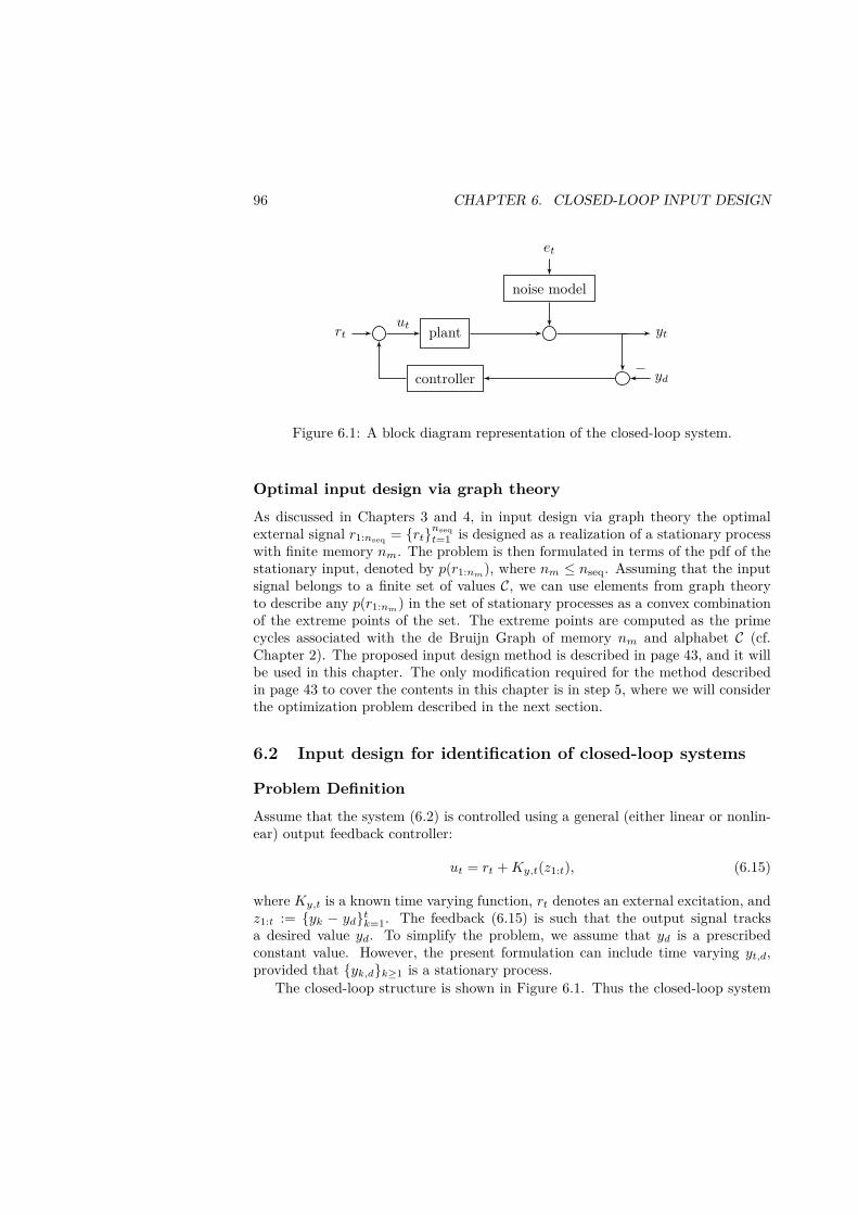
96 CHAPTER 6. CLOSED-LOOP INPUT DESIGN
et
noise model
rt plant yt
controller yd
ut
−
Figure 6.1: A block diagram representation of the closed-loop system.
Optimal input design via graph theory
As discussed in Chapters 3 and 4, in input design via graph theory the optimalexternal signal r1:nseq = rtnseq
t=1 is designed as a realization of a stationary processwith finite memory nm. The problem is then formulated in terms of the pdf of thestationary input, denoted by p(r1:nm
), where nm ≤ nseq. Assuming that the inputsignal belongs to a finite set of values C, we can use elements from graph theoryto describe any p(r1:nm
) in the set of stationary processes as a convex combinationof the extreme points of the set. The extreme points are computed as the primecycles associated with the de Bruijn Graph of memory nm and alphabet C (cf.Chapter 2). The proposed input design method is described in page 43, and it willbe used in this chapter. The only modification required for the method describedin page 43 to cover the contents in this chapter is in step 5, where we will considerthe optimization problem described in the next section.
6.2 Input design for identification of closed-loop systems
Problem Definition
Assume that the system (6.2) is controlled using a general (either linear or nonlin-ear) output feedback controller:
ut = rt +Ky,t(z1:t), (6.15)
where Ky,t is a known time varying function, rt denotes an external excitation, andz1:t := yk − ydtk=1. The feedback (6.15) is such that the output signal tracksa desired value yd. To simplify the problem, we assume that yd is a prescribedconstant value. However, the present formulation can include time varying yt,d,provided that yk,dk≥1 is a stationary process.
The closed-loop structure is shown in Figure 6.1. Thus the closed-loop system

6.2. INPUT DESIGN FOR FEEDBACK SYSTEMS 97
will be
xt+1 = Ft(θ, xt, z1:t) +B(θ)rt,
yt = C(θ)xt + νt,(6.16)
where νt = H(q; θ)et, and
Ft(θ, xt, z1:t) := A(θ)xt +B(θ)Ky,t(z1:t). (6.17)
We assume that the resulting closed-loop system (6.16) is asymptotically stable.
Remark 6.1 If (6.16) is asymptotically stable, and the feedback controller is lin-ear, then the information regarding closed-loop stability can be included in the prob-lem formulation by using the Youla parameterization. Since we know that the closed-loop is stable, then we can parameterize the model structure for the system in theset of linear time invariant models that can be stabilized by the given controller,which is performed by using the Youla parameter [90].
The objective is to design an experiment for the closed-loop system (6.16), thatgenerates nseq samples of the reference signal rt, to be used for identification of theunknown parameters θ in (6.2). To this end, we consider the experiment designproblem (6.14). Since the system is in closed-loop we need to keep the output ofthe plant yt close to yd during the identification experiment. Hence, we chooseto minimize the following experimental cost in the optimal input design problem(6.14)
J = E
nseq∑
t=1
‖yt − yd‖2Q + ‖∆ut‖2
R
, (6.18)
where∆ut := ut − ut−1, (6.19)
and Q and R are positive definite matrices. The first term in (6.18) penalizesthe deviations from the desired output, while the second term is responsible forminimizing the input energy. The expected value in equation (6.18) is with respectto rt and et.
In practical applications, it is common to have bounds on the maximal inputand output amplitudes allowed by the process. These constraints appear due tophysical limitations and/or to keep the system in a safe operating point. However,these bounds cannot be prescribed in a deterministic sense, since both the input andoutput of the system contains a stochastic process that cannot be measured by theuser. Therefore, it is necessary to quantify the input and output constraints by usinga probability measure. Thus, we consider the following probabilistic constraintsduring the identification process1:
P|yt − yd| ≤ ymax > 1 − ǫy, t = 1, . . . , nseq,
P|ut| ≤ umax > 1 − ǫx, t = 1, . . . , nseq,(6.20)
1In equation (6.20) we consider absolute value and the inequality as element-wise operations.
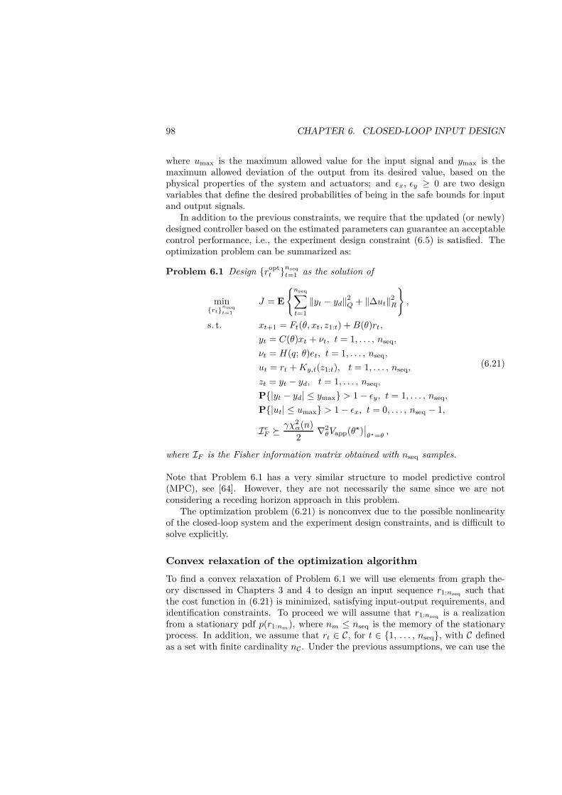
98 CHAPTER 6. CLOSED-LOOP INPUT DESIGN
where umax is the maximum allowed value for the input signal and ymax is themaximum allowed deviation of the output from its desired value, based on thephysical properties of the system and actuators; and ǫx, ǫy ≥ 0 are two designvariables that define the desired probabilities of being in the safe bounds for inputand output signals.
In addition to the previous constraints, we require that the updated (or newly)designed controller based on the estimated parameters can guarantee an acceptablecontrol performance, i.e., the experiment design constraint (6.5) is satisfied. Theoptimization problem can be summarized as:
Problem 6.1 Design roptt nseq
t=1 as the solution of
minrtnseq
t=1
J = E
nseq∑
t=1
‖yt − yd‖2Q + ‖∆ut‖2
R
,
s. t. xt+1 = Ft(θ, xt, z1:t) +B(θ)rt,
yt = C(θ)xt + νt, t = 1, . . . , nseq,
νt = H(q; θ)et, t = 1, . . . , nseq,
ut = rt +Ky,t(z1:t), t = 1, . . . , nseq,
zt = yt − yd, t = 1, . . . , nseq,
P|yt − yd| ≤ ymax > 1 − ǫy, t = 1, . . . , nseq,
P|ut| ≤ umax > 1 − ǫx, t = 0, . . . , nseq − 1,
IeF γχ2α(n)
2∇2θVapp(θ⋆)
∣∣θ⋆=θ
,
(6.21)
where IF is the Fisher information matrix obtained with nseq samples.
Note that Problem 6.1 has a very similar structure to model predictive control(MPC), see [64]. However, they are not necessarily the same since we are notconsidering a receding horizon approach in this problem.
The optimization problem (6.21) is nonconvex due to the possible nonlinearityof the closed-loop system and the experiment design constraints, and is difficult tosolve explicitly.
Convex relaxation of the optimization algorithm
To find a convex relaxation of Problem 6.1 we will use elements from graph the-ory discussed in Chapters 3 and 4 to design an input sequence r1:nseq such thatthe cost function in (6.21) is minimized, satisfying input-output requirements, andidentification constraints. To proceed we will assume that r1:nseq is a realizationfrom a stationary pdf p(r1:nm
), where nm ≤ nseq is the memory of the stationaryprocess. In addition, we assume that rt ∈ C, for t ∈ 1, . . . , nseq, with C definedas a set with finite cardinality nC . Under the previous assumptions, we can use the

6.2. INPUT DESIGN FOR FEEDBACK SYSTEMS 99
methods introduced in Chapters 3 and 4 to define the set of feasible pdfs p(r1:nm)
as a convex combination of its extreme points. The extreme points are computed asthe prime cycles associated with the de Bruijn graph of memory nm and alphabetC (cf. Theorem 2.1 in page 28).
If the set of probability mass functions associated with the extreme points isgiven by pjnv
j=1, then the optimization problem can be rewritten as
minβ1, ..., βnv
J =
nseq∑
t=1
nv∑
j=1
βjEet,r(j)t
∥∥∥y(j)t − yd
∥∥∥2
Q+∥∥∥∆u
(j)t
∥∥∥2
R
,
s.t. x(j)t+1 = Ft(θ, x
(j)t , z
(j)1:t ) +B(θ)r
(j)t ,
y(j)t = C(θ)x
(j)t + νt, t = 1, . . . , nseq,
νt = H(q; θ)et, t = 1, . . . , nseq,
u(j)t = r
(j)t −Ky,t(z
(j)1:t ), t = 1, . . . , nseq,
z(j)t = y
(j)t − yd, t = 1, . . . , nseq,
nv∑
j=1
βjPet,r(j)t
|u(j)t | ≤ umax > 1 − ǫx,
nv∑
j=1
βjPet,r(j)t
|y(j)t − yd| ≤ ymax > 1 − ǫy,
nv∑
j=1
βj I(j)F γχ2
α(n)
2nseq∇2θVapp(θ⋆)
∣∣θ⋆=θ
,
nv∑
j=1
βj = 1, βj ≥ 0, j = 1, . . . , nv. (6.22)
In the minimization problem (6.22), r(j)1:nseq
, u(j)1:nseq
, x(j)1:nseq
, y(j)1:nseq
, and z(j)1:nseq
denote
the signals obtained when r(j)1:nseq
is drawn from pj , j ∈ 1, . . . , nv. The objective of
the optimization problem (6.22) is to minimize the cost J by finding the normalizedweights βjnv
j=1 satisfying the probabilistic bounds in the input and output, and therequirement on the accuracy of the parameter estimates. The first five equationsin the constraints of (6.22) are the equations given by the closed loop system,
which are defined for the external excitations r(j)1:nseq
nv
j=1. The following equationsrepresent the probabilistic bounds for the input and the output, the constrainton the accuracy of the parameter estimates, and the requirement that βjnv
j=1
are nonnegative, normalized weights. We notice that the probabilistic bounds,and the requirement on the accuracy of the parameter estimates are expressed asconvex combination of the respective quantities achieved by the external excitations
r(j)1:nseq
nv
j=1.

100 CHAPTER 6. CLOSED-LOOP INPUT DESIGN
If we denote by βoptj nv
j=1 the set of weighting factors minimizing (6.22), thenthe optimal pdf is given by
popt :=
nv∑
j=1
βoptj pj . (6.23)
Since the set pjnv
j=1 is known (each pj is a uniform distribution over the nodes in
the j-th prime cycle, cf. Theorem 2.1 in page 28), we can sample r(j)t Nsim
t=1 fromeach pj (with Nsim sufficiently large), and numerically approximate the expectedvalues E
et,r(j)t
·, the probabilities Pet,r
(j)t
·, and the corresponding information
matrices I(j)F . This approach is based on Chapters 3 and 4, where numerical sim-
ulations are employed to compute the information matrices associated with each
measure in the set pjnv
j=1. Indeed, given r(j)t Nsim
t=1 and etNsimt=1 , we can generate
y(j)t Nsim
t=1 and u(j)t Nsim
t=1 using (6.16). Therefore, we can compute the expressionsin (6.22) for each j ∈ 1, . . . , nv as
Pet,r
(j)t
|y(j)t − yd| ≤ ymax ≈ 1
Nsim
Nsim∑
t=1
1|y(j)t
|≤ymax,
Pet,r
(j)t
|u(j)t | ≤ umax ≈ 1
Nsim
Nsim∑
t=1
1|u(j)t
|≤umax,
Eet,r
(j)t
∥∥∥y(j)t − yd
∥∥∥2
Q+∥∥∥∆u
(j)t
∥∥∥2
R
≈ 1
Nsim
Nsim∑
t=1
∥∥∥y(j)t − yd
∥∥∥2
Q+∥∥∥∆u
(j)t
∥∥∥2
R
,
where 1X = 1 if X is true, and 0 otherwise, and ∆u(j)t = u
(j)t − u
(j)t−1. The
computation of I(j)F is analyzed in the next subsection.
The key property of the proposed approach is that the input-output constraintsand the restriction on the Fisher information matrix are convex in βjnv
j=1. There-fore, the final optimization problem becomes convex in βjnv
j=1.
Computation of the Fisher information matrix
To integrate the experiment design constraint with the optimization problem (6.22),
we need to compute the Fisher information matrix I(j)F for each r(j)
t nseq
t=1 associatedwith the j-th extreme point of the set of stationary processes of memory nm andalphabet C.
We recall that the Fisher information matrix is given by (cf. Equation (4.3a) inChapter 4)
IF := E
∂ log pθ(y1:nseq)
∂θ
∣∣∣∣θ=θ0
∂ log pθ(y1:nseq)
∂θ⊤
∣∣∣∣θ=θ0
∈ Rnθ×nθ , (6.24)

6.2. INPUT DESIGN FOR FEEDBACK SYSTEMS 101
or equivalently,
IF = −E
∂2 log pθ(y1:nseq)
∂θ∂θ⊤
∣∣∣∣θ=θ0
∈ Rnθ×nθ . (6.25)
where y1:nseq = ytnseq
t=1 . In equations (6.24) and (6.25) the expected value is withrespect to rt and et.
Due to the randomness of et, (6.16) can be rewritten as
xt+1 ∼ fθ(xt+1|y1:t, xt, rt) ,
yt ∼ gθ(yt|xt) ,(6.26)
where fθ(xt+1|y1:t, xt, rt) and gθ(yt|xt) denotes the pdf of the state xt+1, and outputyt, conditioned on the knowledge of xt, rt and y1:t.
Using the model description (6.26), and the Markov property of the system(6.16), we can write the log-likelihood of the joint distribution of y1:nseq and x1:nseq
as (cf. Section 4.1)
log pθ(x1:nseq , y1:nseq) =
nseq−1∑
t=1
logfθ(xt+1|y1:t, xt, rt)
+
nseq∑
t=1
loggθ(yt|xt) + logpθ(x1) . (6.27)
To simplify the computations, we will assume that the distribution of the initialstate is independent of θ, i.e., pθ(x1) = p(x1).
Linear feedback
When Ky,t is a linear controller, expressions (6.24) and (6.25) can be computed
in the frequency domain [59, Section 9.4]. Since we know r(j)t for each j ∈
1, . . . , nv, it is possible to compute its corresponding spectrum, say Φ(j)r (ω). To
this end, we notice that r(j)t is a periodic sequence with period given by Tj . Using
[59, Example 2.3] we compute Φ(j)r (ω) as
Φ(j)r (ω) =
2π
Tj
Tj−1∑
k=0
Φ(j),pr (2πk/Tj)δ(ω − 2πk/Tj) , 0 ≤ ω < 2π , (6.28)
where
Φ(j), pr (ω) :=
Tj−1∑
τ=0
R(j)r (τ)eiωτ , (6.29)
R(j)r (τ) :=
1
Tj
Tj∑
t=1
r(j)t
(r
(j)t−τ
)⊤. (6.30)

102 CHAPTER 6. CLOSED-LOOP INPUT DESIGN
Nonlinear feedback
When Ky is a nonlinear function, equations (6.24) and (6.25) often result in complex(and almost intractable) expressions. Thus, we will approximate the Fisher infor-mation matrix using numerical methods. One solution is to use particle methodsto approximate (6.24) as the covariance matrix of the gradient of the log-likelihoodfunction, ∇θ log pθ(y1:nseq) (score function) (cf. Chapter 4, Subsection 4.3 [86]).In this case, the score function is estimated using the fixed-lag smoother, and theFisher information matrix is approximated as the sample covariance matrix overthe different realizations of ∇θ log pθ(y1:nseq). Another approach is based on thenumerical computation of (6.25) using small perturbation methods [82], where theHessian (6.25) is computed as an average of numerical approximations based on thescore function. The details of the small perturbation method are provided in thenext part.
Computing the information matrix using the small perturbationmethod
Consider the Fisher information matrix given by (6.25). Our goal is to obtainan estimate of (6.25) using the small perturbation method. We use the smallperturbation method since it is simple to implement, and that it can approximate(6.25) even if the gradient of the function is not available. In this section wedescribed the technique in [82] to approximate (6.25).
The main idea in [82] is to compute the Hessian (6.25) based on synthetic data,i.e., realizations of yt, and ut are obtained by simulation of the model (6.16)for small perturbations of θ0, using realizations of rt and et. We will denotethe i-th synthetic data as ZNsim
(i) = y(i), t, u(i), t, r(i), t, e(i), tNsimt=1 , i ∈ 1, . . . , N.
Before we continue, we define ∆(k, i) ∈ Rnθ as a zero mean random vector suchthat its entries are independent, identically distributed, symmetrically distributedrandom variables that are uniformly bounded and satisfy E∆−1
(k, i), l < ∞, with
∆(k, i), l denoting the l-th entry of ∆(k, i). We notice that the latter conditionexcludes uniform and Gaussian distributions. Furthermore, we assume that ∆(k, i), l
are bounded in magnitude. A valid choice is the Bernoulli distribution, defined on−1, 1, and with parameter η = 0.5.
On the other hand, for each realization ZNsim
(i) , we compute the k-th approxima-
tion of (6.25) (k ∈ 1, . . . , M) as
I(k, i)F := −1
2
δG(k, i)
2c
(∆−1
(k, i)
)⊤+ ∆−1
(k, i)
δG⊤(k, i)
2c
, (6.31)
where ,
δG(k, i) := ∇θ log pθ(y(i), 1:Nsim)∣∣θ=θ0+c∆(k, i)
− ∇θ log pθ(y(i), 1:Nsim)∣∣θ=θ0−c∆(k, i)
(6.32)

6.3. NUMERICAL EXAMPLE 103
∆−1(k, i) denotes the entry-wise inverse vector of ∆(k, i), y(i), 1:Nsim
= y(i), tNsimt=1 , and
c > 0 is a predefined constant. In [81] is shown that, under suitable assumptions,the bias of the Fisher information matrix estimate (6.31) is of order O(c2). Themain assumption in [81] is the smoothness of log pθ(y1:Nsim), which is reflectedin the assumption that ∇θ log pθ(y1:Nsim) is thrice continuously differentiable in aneighbourhood of θ0. However, the main limitation of (6.31) is that it is a low rank
approximation of the Fisher information matrix (I(k, i)F has at most rank two), and
it may not even be positive semi-definite.In [82] an improved estimate of the Fisher information matrix is provided as a
function of (6.31). To this end, we define D(k, i) ∈ Rnθ×nθ as
D(k, i) := ∆(k, i)
(∆−1
(k, i)
)⊤− I , (6.33)
and the function Ψ(k, i) : Rnθ×nθ → Rnθ×nθ as
Ψ(k, i)(H) :=1
2HD(k, i) +
1
2D⊤
(k, i)H . (6.34)
Based on (6.33) and (6.34), we can write the new Fisher information matrix estimatein recursive form (in i) as
I(M, i)
F =i− 1
iI(M, i−1)
F +1
iM
M∑
k=1
[I(k, i)F + Ψ(k, i)
(I(M, i−1)
F
)], (6.35)
where I(M, 0)
F = 0. In [82] is shown that the estimate (6.35) tends to IF + O(c2)as N → ∞ (for a fixed M) in mean square sense. The advantage of using theestimator (6.35) over (6.31) is that (6.35) guarantees that the estimate will be afull rank and positive-definite matrix.
6.3 Numerical example
To illustrate the previous discussion, we introduce the following example:
Example 6.1 Consider the open-loop, SISO state space system described by
xt+1 = θ02 xt + ut , (6.36a)
yt = θ01 xt + et , (6.36b)
with true parameters θ0 =[θ0
1 θ02
]⊤=[0.6 0.9
]⊤. The system is controlled in
closed-loop using the controller
ut = rt − ky yt , (6.37)

104 CHAPTER 6. CLOSED-LOOP INPUT DESIGN
0 20 40 60 80 100−0.5
0
0.5
rt
0 20 40 60 80 100−0.5
0
0.5
rt
0 20 40 60 80 100−0.5
0
0.5
t
rt
Figure 6.2: Part of the reference signal rt500t=1. Top: Optimal reference signal.
Middle: Optimal reference signal without probabilistic constraints. Bottom: Ran-dom binary signal.
where ky = 0.5 is a known constant. The objective is to identify the open-loop
parameters θ =[θ1 θ2
]⊤from the identified closed-loop ones θc =
[θc1 θc2
]⊤in
the model
xt+1 = θc2 xt + rt − ky et , (6.38a)
yt = θc1 xt + et , (6.38b)
using the transformation law
θ1 = θc1 , (6.39a)
θ2 = θc1 + ky θc1 . (6.39b)
To this end, we will design the reference signal rt500t=1 as a realization of a station-
ary process with memory nm = 2, and subject to rt ∈ C = −0.5, −0.25, 0, 0.25, 0.5,for all t ∈ 1, . . . , 500. Since the experiment will be performed in closed-loop, we

6.3. NUMERICAL EXAMPLE 105
0 20 40 60 80 100
−1
1
ut
0 20 40 60 80 100
−1
1
ut
0 20 40 60 80 100
−1
1
t
ut
Figure 6.3: Part of the input signal ut500t=1. Top: Input signal for the optimal
reference. Middle: Input signal for the optimal reference without probabilisticconstraints. Bottom: Input signal for a random binary reference.
define the following cost function to measure performance degradation:
Vapp(θ) =1
500
500∑
t=1
‖yt(θ0) − yt(θ)‖22 , (6.40)
where yt(θ) denotes the closed-loop output when θ is employed to describe the openloop model and a linear output feedback controller with constant gain ky has beenused. The cost function (6.40) is used to build the application set as in (6.9).Finally, we will solve the approximate problem (6.22), where yd = 0, for all t ∈1, . . . , 500, Q = 1, R = 0.02, εy = εx = 0.07, ymax = 2, umax = 1, γ = 102, andα = 0.98.
Figure 6.2 presents one realization of rt500t=1 obtained by solving (6.22), one
realization of rt500t=1 obtained by solving (6.22) without probabilistic constraints,
and from a random binary sequence with values −0.5, 0.5. From this figure wesee that the optimal sequence is zero most of the time, except for short pulses.This can be explained from the tight probabilistic bounds imposed for ut, which

106 CHAPTER 6. CLOSED-LOOP INPUT DESIGN
0 20 40 60 80 100
−2
0
2
yt
0 20 40 60 80 100
−2
0
2
yt
0 20 40 60 80 100
−2
0
2
t
yt
Figure 6.4: Part of the output yt500t=1. Top: Output signal for the optimal refer-
ence. Middle: Output signal for the optimal reference without probabilistic con-straints. Bottom: Output signal for a random binary reference.
restricts the excitation provided by rt. If we compare the previous signal with theone obtained by solving (6.22) without probabilistic bounds, we see that the referencesignal contains more oscillations when the probabilistic bounds are removed.
Figures 6.3 and 6.4 present one realization for the resulting input ut500t=1 and
output yt500t=1, respectively. From those realizations, we conclude that, for the
optimal reference, the input and output are inside the limiting regions 93.8%, and96% of the time, respectively, which satisfies the design requirements. On the otherhand, for the reference signal obtained by solving (6.22) without probabilistic bounds,we have that the input and output satisfies the constraints 86.6% and 93.4% of thetime, respectively. Therefore, in this example we need to incorporate the probabilisticbounds to guarantee that both the input and output of the system are inside thedesired region with the prescribed confidence level. With the previous modification,we restrict the set of optimal feasible solutions for the problem of minimum varianceto the subset of optimal solutions satisfying the probabilistic bounds. Finally, for therandom binary reference, we have that the input and output are inside the confidence

6.3. NUMERICAL EXAMPLE 107
0.4 0.6 0.8
0.7
0.8
0.9
1
1.1
θ1
θ2
0.4 0.6 0.8
0.7
0.8
0.9
1
1.1
θ1
θ2
Figure 6.5: Application ellipsoid (green, dot-dashed line) with the respective iden-tification ellipsoids. Blue, continuous line: Identification ellipsoid for the randombinary reference (realizations marked with ∗). Red, continuous line: Identificationellipsoid for the optimal reference with probabilistic bounds (realizations markedwith circles). Black, dashed line: Identification ellipsoid for the optimal referencewithout probabilistic bounds (realizations marked with triangles).
region 90.8%, and 79.6% of the time, which does not satisfy the confidence boundsfor the system.
To analyze the identification performance, Figure 6.5 presents the applicationellipsoid for the parameter θ, together with the resulting identification ellipsoidsand 50 identified parameters obtained with the optimal reference with probabilis-tic bounds, the optimal reference without probabilistic bounds, and for the randombinary reference. From this figure we conclude that the 98% confidence level setfor the identified parameters lies completely inside the application ellipsoid for allthe reference signals. As expected, the confidence level set for the random binaryreference is smaller than the ones obtained with the proposed technique, since thevariance of this signal is greater than the one obtained with the optimal references.Hence, the random binary reference excites the system more than required, whichmakes the cost function in optimization problem (6.21) greater than the cost ob-tained with the proposed method. Indeed, the cost functions are Jopt = 541.6 forthe optimal experiment with probabilistic bounds, and Jbinary = 695.8 for a randombinary reference, which is in line with the size of the uncertainty ellipsoids in Fig-ure 6.5. On the other hand, we see that the confidence ellipsoids for the estimatedparameters are almost the same when a reference signal is designed by including orexcluding the probabilistic bounds on the input and output.

108 CHAPTER 6. CLOSED-LOOP INPUT DESIGN
6.4 Conclusion
In this chapter a method to design input sequences for closed-loop experimentshas been proposed. The method considers the input sequence as a realization of astationary process minimizing the experimental cost, and subject to performanceconstraints. Using the graph-theoretical approach presented in Chapters 2-4, wecan express both experimental cost and constraints as a convex combination ofthe values associated with the extreme measures in the set of stationary processeswith finite alphabet and memory, which are computed using numerical methods.An interesting feature of this approach is that probabilistic constraints becomeconvex in the decision variables. The numerical example shows that this approachis an attractive method for the design of input sequences to identify models in aclosed-loop setting.

Chapter 7
Conclusions
In this thesis we have introduced a new approach to input design for system identifi-cation. The results presented in this thesis can be seen as an extension of the resultsin [54] and [6, 7]. The main difference with [6, 7] is that we optimize over the sta-tionary probability mass function (pmf) associated with the Markov chain, insteadof directly optimizing over the transition probabilities, which results in a convexproblem. On the other hand, this thesis covers the optimal input design problemfor identification of nonlinear output error and nonlinear state space models, whichextends the nonlinear FIR model structure considered in [54].
The proposed technique considers the optimization of an input sequence as arealization of a stationary process with finite memory and finite alphabet, whichmaximizes a scalar cost function of the Fisher information matrix. By using notionsof graph theory, it is possible to characterize the set of stationary probability massfunctions (pmfs) through its extreme points. It has been proved that the extremepoints of the set of stationary processes are in one to one correspondence with theprime cycles in the equivalent de Bruijn graph.
Once the prime cycles are computed, the probability measures associated withthe extreme points of the set of stationary processes are known. Furthermore,an input sequence can be drawn from each prime cycle, which can be employedto compute a numerical approximation of the Fisher information matrix for eachextreme point in the set. Therefore, the Fisher information matrix can be computedwith a prescribed accuracy even if closed form expressions are not available, whichmakes the proposed input design method suitable for nonlinear model structures.The Fisher information matrices computed for the extreme points are then used tosolve the input design problem by finding the optimal convex combination of thegiven matrices. Thus, the input design problem becomes convex even for nonlinearmodel structures.
The solution of the input design problem delivers the optimal stationary pmfassociated with the optimal cost function, from which an input sequence must besampled. The problem of obtaining a sample from a prescribed stationary pmf
109

110 CHAPTER 7. CONCLUSIONS
can be solved by using Markov chains, where the input samples are obtained asthe states of the chain. Provided that the Markov chain is ergodic, the inputsamples will tend to be distributed according to the stationary distribution of theMarkov chain. The existing results on the design of Markov chains with a prescribedstationary distribution lie on the properties of the associated graph and/or thestationary pmf (e.g., undirected graphs, or reversible Markov chains), which arenot applicable to the present work. Therefore, this thesis also introduces a methodfor designing Markov chains for de Bruijn graphs with a prescribed stationary pmf.
As a first approach to input design, we analyze the proposed method for thecase of nonlinear output-error model structures. For this case, it is shown thatthe computation of the Fisher information matrix can be carried out by numeri-cal approximation, where the accuracy of the approximation is controlled directlythrough the number of samples taken from the associated prime cycle. The nu-merical examples show that the method retrieves existing results on input designfor nonlinear FIR model structures, and that it can also be employed for designinginput sequences for identification of more general nonlinear output-error models,which are not covered by previous results in the area.
The major difficulty associated with extending the input design method onChapter 3 to more general nonlinear models is the approximation of the Fisherinformation matrices. As a solution to this issue, Chapter 4 introduced an extensionof the input design method to nonlinear state space models. The extension relieson particle methods, where an approximation of the observed information matrixis computed as the sample covariance matrix of the score function. In this case,the accuracy of the approximation is a trade-off between the number of particles(which increases the accuracy for a fixed data length) and the data length (whichdecreases the accuracy for a fixed number of particles). In order to deal with theuncertainty associated with the approximation method, we consider the solution tothe optimization problem as the sample mean of the different solutions obtainedfor different approximations of the Fisher information matrix.
As applications of the proposed method, this thesis discusses two different prob-lems. The first problem concerns the design of input sequence for model estima-tion in channels with quantized output. Since a numerical approximation for theFisher information matrix associated with the model is available, the problem canbe solved by using the presented method. A simulation example shows that themethod can be employed to obtain more informative experiments compared to theresults obtained by using a realization from a white noise process.
The second application of the method is found on application oriented closed-loop input design. In this case the objective is the design of an external inputsequence to improve the parameters employed for the model of a plant operatingin closed-loop, while guaranteeing limits on the performance degradation duringthe experiment (e.g., probabilistic constraints on the input and output, and confi-dence ellipsoids for the identified parameters). By using the proposed input designmethod, the problem can be solved by using convex optimization tools, where boththe constraints and the cost function are optimized as a convex combination of the

111
extreme points characterizing the set of stationary pmfs.The discussion in this thesis shows that the proposed input design method is
an attractive alternative to design input sequences for identification of nonlinearmodel structures, where the method guarantees a convex optimization problem,which allows to employ powerful tools for solving the optimal input design problem.
Future work
This thesis can be seen as a first approach to input design for identification ofnonlinear models. However, there is plenty of space to improve the results in thisarea. Some ideas for future work in the subject are:
Reduction of computational effort The main limitation of the input designmethod introduced in this thesis is the computational effort needed to obtainthe solution. As discussed in Chapter 2, the computational effort is mostlyrelated with the prime cycles. An approach to overcome this issue is an openquestion and topic of future research.
Irreducibility of the designed Markov chains The generation of an input re-alization from a given stationary pmf relies on the fact that the resultingMarkov chain is irreducible, i.e., there is only one class of states in the chain.The results presented in this thesis do not guarantee that the optimal pmf willbe associated with an irreducible Markov chain, which is important since aninput realization distributed according to the desired pmf is needed in orderto perform the experiment. A possibility to overcome this issue is to forcein the optimization problem the requirement of irreducibility of the Markovchain. Another option for this issue is to reduce the memory of the Markovchain until an irreducible chain is obtained. These options will be analyzedin future research.
Stationary pdfs with continuous support The thesis has focused on the de-sign of input sequences with finite alphabet. An approach to input designwhen the alphabet lies on a continuous support is an open problem and pos-sible research topic.
Robust optimal input design As with most optimal input design methods, theone presented in this thesis considers the existence of prior knowledge aboutthe model parameters. An alternative to overcome this issue is to implementa robust design scheme on top of it, or through an adaptive input designprocedure, where the signal is redesigned as more information is collectedfrom the system.
Application oriented closed-loop experiment design The results obtained inChapter 6 consider a linear model structure for the plant, under a known non-linear feedback. An extension of the method to include implicit feedback laws(e.g., as in model predictive control) is a future research direction in the topic.


Appendices
113


Appendix A
Algorithms for computation of
elementary cycles
In this appendix we present the algorithms implemented in the input design meth-ods of Chapters 2-4.
A.1 Preliminaries
Before introducing the algorithms required in Chapters 2-4, we need the followingdefinitions [84]:
Definition A.1 (Undirected graph) Let G = (V , E) be a graph. Then G is calledan undirected graph if and only if
E = v, w| v, w ∈ V , (A.1)
where v, w is an unordered pair of vertices.
Definition A.2 (Tail and head of an edge) Let G = (V , E) be a directed graph.Given an edge (v, w) ∈ E, v is defined as the tail of the edge (v, w), and w isdefined as the head of the edge (v, w).
Definition A.3 (Undirected version of a directed graph) Let G = (V , E) be a di-rected graph. The undirected version of a directed graph G is defined as the graphformed by converting each edge in E into an undirected edge, and removing duplicateedges.
Definition A.4 (Connected undirected graph) Let G = (V , E) be a undirected graph.Then G is said to be connected if there is a path between every pair of vertices.
Definition A.5 (Tree) A tree T is a directed graph whose undirected version isconnected. In addition, a tree T has one vertex which is the head of no edges (called
115

116 APPENDIX A. ALGORITHMS FOR ELEMENTARY CYCLES
the root), and such that all vertices except the root are head of exactly one edge. If(v, w) is an edge of T , then v is an ancestor of w, and w is a descendant of v.
Definition A.6 (Subtree) Let T be a tree, and v a node in T . Then Tv is thesubtree of T with respect to v if and only if Tv has as vertices all the descendantsof v in T .
Definition A.7 (Spanning tree) Let G = (V , E) be a directed graph. A tree T is aspanning tree of G if T is a subgraph of G, and T contains all the vertices of G.
Definition A.8 (Palm tree) Let G be a directed graph, consisting of two disjointsets of edges, denoted by E1 and E2, respectively. Suppose G satisfies the followingproperties:
(i) The subgraph T containing the edges E1 is a spanning tree of G.
(ii) Each edge which is not in the spanning tree T of P connects a vertex withone of its ancestors in T .
Then G is called a palm tree. The edges E2 are called the fronds of G.
Definition A.9 (Cross-link) Let T be a tree, and assume there are subtrees Tv,Tw in T . Then, the edge (tv, tw) is called a cross-link if and only if tv is in Tv andtw is in Tw.
A.2 Strong connected components of a graph
A term required in the discussion of the algorithms in this thesis is the concept ofstrongly connected graphs, whose definition is given below [84, Definition 4]:
Definition A.10 (Strongly connected graph) Let G = (V , E) be a directed graph.Suppose that for each pair of vertices v, w ∈ G, there exist paths p1 = (v, . . . , w)and p2 = (w, . . . , v). Then G is said to be strongly connected.
Based on Definition A.10, we have the following result [84, Lemma 9]:
Lemma A.1 (Strongly connected components) Let G = (V , E) be a directed graph.We may define an equivalence relation on the set of vertices as follows: two verticesv and w are equivalent if there is a cycle p = (v, . . . , v) which contains w. Let thedistinct equivalence classes under this relation be Vi, i ∈ 1, . . . , n. Let G =(Vi, Ei), where Ei := (u, w) ∈ E : v, w ∈ Vi. Then:
(i) Each Gi is strongly connected.
(ii) No Gi is a proper subgraph of a strongly connected subgraph of G.
Then the subgraphs Gini=1 are called the strongly connected components of G.

A.3. ELEMENTARY CYCLES OF A GRAPH 117
It is shown in [84] that the problem of finding the strongly connected componentsof a graph G can be reduced to the problem of finding the roots of the stronglyconnected components. In this appendix we define LOWLINK(v) as the smallestvertex (according to a user defined indexing for the vertices in G) which is in thesame component as v and is reachable by traversing zero or more tree arcs followedby at most one frond or cross-link. We refer to [84, p. 156] for more details aboutthe definition of this function.
Algorithm A.1 in page 118 presents a pseudo-code for computing the set ofstrongly connected components in a given graph G [84, p. 157]. It is shown in [84]that Algorithm A.1 requires O(V , E) space and time, where
O(V , E) ≤ k1 #V + k2 #E + k3 , (A.2)
for some positive constants k1, k2, and k3.The pseudo-code for determining the set of strongly connected components in
a graph G will be employed in the computation of elementary cycles in G, which isdiscussed in the next section.
A.3 Elementary cycles of a graph
As it is mentioned in Chapter 2, the computation of prime cycles in a graph GCnm
can be performed by finding all the elementary cycles in GCnm−1 . In this sectionwe provide an algorithm to find the set of elementary cycles in a directed graph G.The algorithm is based on the one introduced in [46, pp. 79–80]. The pseudo-codeassociated with this algorithm is presented in Algorithm A.2-A.3.
We describe Algorithm A.2-A.3 based on the discussion provided in [46, p.79]. The algorithm proceeds by building elementary paths from s. The verticesof the current elementary path are kept on a stack. A vertex is appended to anelementary path by a call to the procedure CIRCUIT and is deleted upon returnfrom this call. When a vertex v is appended to a path it is blocked by settingBLOCKED(v) = true, so that v cannot be used twice on the same path. However,when we return from the call which blocks v, v is not necessarily unblocked. Theidea is that we unblock a node with a sufficient delay such that any two unblockingsof v are separated by either an output of a new circuit or a return to the mainprocedure.

118 APPENDIX A. ALGORITHMS FOR ELEMENTARY CYCLES
Algorithm A.1 Computation of strongly connected components in a graph
Inputs: A directed graph G = (V, E).Output: The set of strongly connected components in G.
1: Begin
2: Integer i;3: Procedure STRONGCONNECT(v);4: Begin
5: i := i + 1;6: NUMBER(v) := i;7: LOWLINK(v) := NUMBER(v);8: put v on stack of points;9: For w in the set of descendants Dv do
10: Begin
11: If w is not yet numbered then
12: Begin comment (v, w) is a tree arc;13: STRONGCONNECT(w);14: LOWLINK(v) := minLOWLINK(v), NUMBER(w);15: end
16: Else If NUMBER(w) < NUMBER(v) do
17: Begin comment (v, w) is a frond or cross-link;18: If w is on stack of points then
19: Begin
20: LOWLINK(v) := minLOWLINK(v), NUMBER(w);21: end
22: end
23: end
24: If LOWLINK(v) = NUMBER(v) then
25: Begin comment v is the root of a component;26: start new strongly connected component;27: While w on top of point stack satisfies NUMBER(w) ≥ NUMBER(v) do
28: Begin
29: delete w from point stack and put w in current component;30: end
31: end
32: end
33: i := 0;34: empty stack of points;35: For w a vertex do
36: Begin
37: If w is not yet numbered then
38: Begin
39: STRONGCONNECT(w);40: end
41: end
42: end

A.3. ELEMENTARY CYCLES OF A GRAPH 119
Algorithm A.2 Computation of elementary cycles in a graph (Part I)
Inputs: A directed graph G = (V, E).Output: The set of elementary cycles in G.
1: Begin
2: Integer list array AK(n), B(n);3: Logical array BLOCKED(N);4: Integer s;5: Logical Procedure CIRCUIT(v);6: Begin Logical f ;7: Procedure UNBLOCK(u);8: Begin
9: BLOCKED(u) := false;10: For w ∈ B(u) do
11: Begin
12: delete w from B(u);13: If BLOCKED(w) then
14: Begin
15: UNBLOCK(w);16: end
17: end
18: end
19: f := false;20: stack v;21: BLOCKED(v) := true;22: For w ∈ AK(v) do
23: Begin
24: If w = s then
25: Begin
26: output circuit composed of stack followed by s;27: f := true;28: end
29: Else If BLOCKED(w) = false then
30: Begin
31: If CIRCUIT(w) = true then
32: Begin
33: f := true;34: end
35: end
36: end
37: If f = true then
38: Begin
39: UNBLOCK(v);40: end
41: Else For w ∈ AK(v) do
42: Begin
43: If v /∈ B(w) then
44: Begin
45: put v on B(w);46: end
47: end
48: unstack v;49: CIRCUIT := f ;50: end

120 APPENDIX A. ALGORITHMS FOR ELEMENTARY CYCLES
Algorithm A.3 Computation of elementary cycles in a graph (Part II)
Inputs: A directed graph G = (V, E).Output: The set of elementary cycles in G.
51: empty stack;52: s := 1;53: while s < n do
54: Begin
55: AK := adjacency matrix of strong component K with least vertex in subgraph56: of G induced by s, s + 1, . . . , n;57: If AK 6= ∅ then
58: Begin
59: s := least vertex in VK ;60: For i ∈ VK do
61: Begin
62: BLOCKED(i) := false;63: B(i) := ∅;64: end
65: dummy := CIRCUIT(s);66: s := s + 1;67: end
68: Else
69: Begin
70: s := n;71: end
72: end
73: end

Appendix B
Convergence of the approximation
of IF
In this appendix we prove that the approximation (3.17) in page 42 converges to
I(i)F as Nsim → ∞:
Theorem B.1 If ut has period T satisfying |ut| ≤ K for some K ≥ 0, andψθ0t (ut)ψ
θ0t (ut)
⊤ is exponentially stable, then
limNsim→∞
1
Nsim
Nsim∑
t=1
ψθ0t (ut)ψ
θ0t (ut)
⊤
=1
T
T∑
t=1
ψθ0t (ut)ψ
θ0t (ut)
⊤
=
∫ψθ0t (ut,−∞)ψθ0
t (ut,−∞)⊤ dP (ut,−∞) ,
(B.1)
where ut is equal to ut for t > 0 but ut = 0 for t ≤ 0, ut,−∞ := uktk=−∞,ut,−∞ := uktk=−∞, and P is the probability measure of a Markov chain generatingut (a uniform probability distribution on the set of possible values of u1:T ).
Proof Given ε > 0, take S as a multiple of T such that CδSψ < ε. Then, for everyt > S, ∣∣∣ψθ0
t (ut)ψθ0t (ut)
⊤ − ψθ0t (ut−St )ψθ0
t (ut−St )⊤∣∣∣ < CδSψ < ε . (B.2)
On the other hand, since ut is periodic of period T , ut−St,−∞ takes only a finitenumber of values for t > S (at most S), we have that for Nsim = mS + n (with m,n positive integers |n| ≤ S):
1
Nsim
Nsim∑
t=1
ψθ0t (ut)ψ
θ0t (ut)
⊤ =mS
Nsim
1
mS
[mS∑
t=1
ψθ0t (ut)ψ
θ0t (ut)
⊤
121

122 APPENDIX B. CONVERGENCE OF THE APPROXIMATION OF IF
+
Nsim∑
t=mS+1
ψθ0t (ut)ψ
θ0t (ut)
⊤]
=mS
Nsim
1
mS
mS∑
t=1
[ψθ0t (ut−St )ψθ0
t (ut−St )⊤ + ηt
]+
1
Nsim
Nsim∑
t=mS+1
ψθ0t (ut)ψ
θ0t (ut)
⊤
=mS
Nsim
1
T
T∑
t=1
ψθ0t (ut−St )ψθ0
t (ut−St )⊤ +1
Nsim
mS∑
t=1
[µt + ηt]
+1
Nsim
Nsim∑
t=mS+1
ψθ0t (ut)ψ
θ0t (ut)
⊤ , (B.3)
where µt, ηt ∈ [−ε, ε]. Thus, the second term in (B.3) is bounded by 2ε. Moreover,the third term in (B.3) tends to 0 as Nsim → ∞ (since it consists of a sum of amost S terms). Therefore,
∣∣∣∣∣ limNsim→∞
1
Nsim
Nsim∑
t=1
ψθ0t (ut)ψ
θ0t (ut)
⊤ − 1
T
T∑
t=1
ψθ0t (ut−St )ψθ0
t (ut−St )⊤
∣∣∣∣∣ ≤ 2ε , (B.4)
and since ε was arbitrary, we conclude that
limNsim→∞
1
Nsim
Nsim∑
t=1
ψθ0t (ut)ψ
θ0t (ut)
⊤ =1
T
T∑
t=1
ψθ0t (ut−St )ψθ0
t (ut−St )⊤ . (B.5)
The last equality in (B.1) follows since P assigns equal probability to T differentsequences (corresponding to the possible sequences obtained by shifting ut).

Appendix C
The expectation-maximization
algorithm
In this appendix we present the expectation-maximization algorithm, and usefulidentities for the methods discussed in Chapter 4. The material in this appendix isbased on [8, 76, 77].
C.1 The expectation-maximization algorithm
The expectation-maximization (EM) algorithm [20, 66] is an iterative procedurethat at the k-th step seeks a value θk such that the likelihood is increased in thesense that log pθk
(y1:T ) > log pθk−1(y1:T ).
The main idea of the EM algorithm is the postulation of a missing data setx1:T . In this thesis, the missing data x1:T will be understood as the state se-quence in the model structure (1.3) in page 3, but other choices are possible, andit can be considered as a design variable. Thus, we consider the joint log-likelihoodfunction log pθ(x1:T , y1:T ) with respect to both the observed data y1:T and themissing data x1:T . This approach assumes that maximizing the joint log-likelihoodlog pθ(x1:T , y1:T ) is easier than maximizing the marginal one log pθ(y1:T ).
The EM algorithm then copes with x1:T being unavailable by forming an ap-proximation Q(θ, θk) of log pθ(x1:T , y1:T ). The approximation used is the minimumvariance estimate of log pθ(x1:T , y1:T ) given the observed data y1:T , and an assump-tion θk of the true parameter value. This minimum variance estimate is given bythe conditional expectation [2]:
Q(θ, θk) := E log pθ(x1:T , y1:T )| y1:T
=
∫
X1:T
log pθ(x1:T , y1:T )pθk(x1:T |y1:T ) dx1:T . (C.1)
The utility of this approach depends on the relationship between log pθ(y1:T ), andthe approximation Q(θ, θk) of log pθ(x1:T , y1:T ). This can be examined by using
123

124 APPENDIX C. THE EM ALGORITHM
the definition of conditional probability to write
log pθ(x1:T , y1:T ) = log pθ(x1:T |y1:T ) + log pθ(y1:T ) . (C.2)
Taking the conditional expectation E·|y1:T on both sides of equation (C.2) weobtain
Q(θ, θk) = log pθ(y1:T ) +
∫
X1:T
log pθ(x1:T |y1:T )pθk(x1:T |y1:T ) dx1:T . (C.3)
Therefore,
log pθ(y1:T ) − log pθk(y1:T ) = Q(θ, θk) − Q(θk, θk)
+
∫
X1:T
logpθk
(x1:T |y1:T )
pθ(x1:T |y1:T )pθk
(x1:T |y1:T ) dx1:T . (C.4)
The integral in the right hand side of the equality in (C.4) is known as the Kullback-Leibler divergence metric, which is non-negative. Indeed, for x > 0 we have− log x ≥ 1 − x, which implies
−∫
X1:T
logpθ(x1:T |y1:T )
pθk(x1:T |y1:T )
pθk(x1:T |y1:T ) dx1:T
≥∫
X1:T
(1 − pθ(x1:T |y1:T )
pθk(x1:T |y1:T )
)pθk
(x1:T |y1:T ) dx1:T = 0 , (C.5)
where the equality to zero is due to the fact that pθ(x1:T |y1:T ) is of unit area forany value of θ. As a consequence of (C.5) we have that
log pθ(y1:T ) − log pθk(y1:T ) ≥ Q(θ, θk) − Q(θk, θk) . (C.6)
Equation (C.6) is the key of the EM algorithm. Namely, choosing θ so thatQ(θ, θk) > Q(θk, θk) implies that the log-likelihood is also increased in that
log pθ(y1:T ) > log pθk(y1:T ).
The EM algorithm exploits this to deliver a sequence of values θk designed tobe increasingly good approximations of the maximum likelihood estimate (1.5) inpage 5. Algorithm C.1 summarizes the steps in the EM method.
Remark C.1 For reference in the next sections, we define
H(θ, θ′) := −∫
X1:T
log pθ(x1:T |y1:T )pθ′(x1:T |y1:T ) dx1:T . (C.8)

C.2. EM ALGORITHM: USEFUL IDENTITIES 125
Algorithm C.1 EM algorithm
Inputs: y1:T (observations), and log pθ(x1:T , y1:T ) (joint log-likelihood function).Output: θT (parameter estimate).
1: Set k = 0 and initialize θk such that log pθ(y1:T ) is finite.2: (Expectation (E) step): Compute Q(θ, θk).3: (Maximization (M) step): Compute
θk+1 = arg maxθ∈Θ
Q(θ, θk) . (C.7)
4: If not converged, update k = k + 1 and return to line 2. Otherwise, set θT = θk+1,and stop the algorithm.
C.2 EM algorithm: useful identities
In this section we introduce useful results that can be derived from the intermedi-ate expressions for the EM algorithm. In particular, we present the Fisher’s andLouis’ identities, which are employed to estimate the Fisher information matrix inChapter 4. To this end, we need the following assumption [8]:
Assumption C.1 Assume that the following conditions hold:
(i) The parameter Θ is an open subset of Rnθ (for some integer nθ).
(ii) For any θ ∈ Θ, pθ(y1:T ) is positive and finite.
(iii) For any (θ, θ′) ∈ Θ × Θ,
∫
X1:T
|log pθ(x1:T |y1:T )| pθ′(x1:T |y1:T ) dx1:T ,
is finite.
(iv) pθ(y1:T ) is twice continuously differentiable on Θ.
(v) For any θ′ ∈ Θ, θ → H(θ, θ′) is twice continuously differentiable on Θ. Inaddition, ∫
X1:T
∣∣∇kθ log pθ(x1:T |y1:T )
∣∣ pθ′(x1:T |y1:T ) dx1:T ,
is finite for k = 1, 2 and any (θ, θ′) ∈ Θ × Θ, and
∇kθ
∫
X1:T
log pθ(x1:T |y1:T )pθ′(x1:T |y1:T ) dx1:T
=
∫
X1:T
∇kθ log pθ(x1:T |y1:T )pθ′(x1:T |y1:T ) dx1:T .

126 APPENDIX C. THE EM ALGORITHM
Fisher’s identity
A result derived from the EM algorithm is known as the Fisher’s identity [8, 25]:
Theorem C.1 Consider that Assumption C.1 holds. then:
∇θ log pθ(y1:T )|θ=θ′ =
∫
X1:T
∇θ log pθ(x1:T , y1:T )|θ=θ′ pθ′(x1:T |y1:T ) dx1:T , (C.9)
and
− ∇2θ log pθ(y1:T )
∣∣θ=θ′ =
−∫
X1:T
∇2θ log pθ(x1:T , y1:T )
∣∣θ=θ′ pθ′(x1:T |y1:T ) dx1:T
+
∫
X1:T
∇2θ log pθ(x1:T |y1:T )
∣∣θ=θ′ pθ′(x1:T |y1:T ) dx1:T . (C.10)
Proof Expression (C.9) is (C.1) differentiated once under the integral sign (using(C.3)), and expression (C.10) is (C.3) differentiated twice under the integral sign.
Remark C.2 Expression (C.9) is known as Fisher’s identity, and equation (C.10)is normally referred to as the missing information principle [62].
Louis’ identity
The second result useful in this thesis is known as Louis’ identity [8, 62]:
Theorem C.2 (Louis’ identity) Consider that Assumption C.1 holds. Then:
∇2θ log pθ(y1:T )
∣∣θ=θ′ + ∇θ log pθ(y1:T )|θ=θ′ ∇θ log pθ(y1:T )|θ=θ′⊤
=∫
X1:T
[∇2θ log pθ(x1:T , y1:T )
∣∣θ=θ′
+ ∇θ log pθ(x1:T , y1:T )|θ=θ′ ∇θ log pθ(x1:T , y1:T )|θ=θ′⊤]pθ′(x1:T |y1:T ) dx1:T .
(C.11)
Proof To prove (C.11), we start from (C.10) and note that the second term onthe right-hand side of the equality is the negative of an information matrix for theparameter θ associated with the probability density function pθ(·|y1:T ) evaluated atθ = θ′. Therefore, we can use the information matrix identity
∫
X1:T
∇2θ log pθ(x1:T |y1:T )
∣∣θ=θ′ pθ′(x1:T |y1:T ) dx1:T =

C.2. EM ALGORITHM: USEFUL IDENTITIES 127
−∫
X1:T
∇θ log pθ(x1:T |y1:T )|θ=θ′
∇θ log pθ(x1:T |y1:T )|θ=θ′⊤pθ′(x1:T |y1:T ) dx1:T . (C.12)
This is a consequence of Assumption C.1, point (v), and the fact that pθ(·|y1:T ) isa probability density function for all values of θ, implying that
∫
X1:T
∇θ log pθ(x1:T |y1:T )|θ=θ′ pθ′(x1:T |y1:T ) dx1:T = 0 . (C.13)
Using the identity (C.2), and (C.9) we conclude that
∫
X1:T
∇θ log pθ(x1:T |y1:T )|θ=θ′
∇θ log pθ(x1:T |y1:T )|θ=θ′⊤pθ′(x1:T |y1:T ) dx1:T =
∫
X1:T
∇θ log pθ(x1:T , y1:T )|θ=θ′
∇θ log pθ(x1:T , y1:T )|θ=θ′⊤pθ′(x1:T |y1:T ) dx1:T
+ ∇θ log pθ(y1:T )|θ=θ′ ∇θ log pθ(y1:T )|θ=θ′⊤ , (C.14)
which completes the proof.


Bibliography
[1] J.C. Agüero, W. Tang, J.I. Yuz, R. Delgado, and G.C. Goodwin. Dual time-frequency domain system identification. Automatica, 48(12):3031–3041, 2012.
[2] B.D.O. Anderson and J.B. Moore. Optimal filtering. Prentice Hall, EnglewoodCliffs, N.J., 1979.
[3] X. Bombois, G. Scorletti, M. Gevers, P.M.J. Van den Hof, and R. Hildebrand.Least costly identification experiment for control. Automatica, 42(10):1651–1662, October 2006.
[4] S. Boyd, P. Diaconis, and L. Xiao. Fastest mixing Markov chain on a graph.SIAM Review, 46(4):667–689, October 2004.
[5] S. Boyd and L. Vandenberghe. Convex Optimization. Cambridge UniversityPress, 2004.
[6] C. Brighenti. On input design for system identification: input design usingMarkov chains, M.Sc. Thesis, KTH Royal Institute of Technology, Stockholm,Sweden, 2009.
[7] C. Brighenti, B. Wahlberg, and C.R. Rojas. Input design using Markov chainsfor system identification. In Joint 48th Conference on Decision and Controland 28th Chinese Conference, pages 1557–1562, Shangai, P.R. China, 2009.
[8] O. Cappé, E. Moulines, and T. Rydén. Inference in Hidden Markov Models.Springer, 2005.
[9] G. Casella and R.L. Berger. Statistical inference. Duxbury Pacific Grove,CA, 2002.
[10] M. Casini, A. Garulli, and A. Vicino. Input design for worst-case system iden-tification with uniformly quantized measurements. In 15th IFAC Symposiumon System Identification (SYSID), Saint-Malo, France, 2009.
[11] M. Casini, A. Garulli, and A. Vicino. Input design in worst-case systemidentification using binary sensors. IEEE Transactions on Automatic Control,56(5):1186–1191, 2011.
129

130 BIBLIOGRAPHY
[12] M. Casini, A. Garulli, and A. Vicino. Input design in worst-case systemidentification with quantized measurements. Automatica, 48(5):2297–3007,2012.
[13] B. Chen and P.K. Willett. Channel optimized binary quantizers for dis-tributed sensor networks. In Proceedings of the IEEE International Confer-ence on Acoustics, Speech, and Signal Processing (ICASSP), volume 3, pages(iii) 845–848. IEEE, 2004.
[14] D.R. Cox. Planning of experiments. New York: Wiley, 1958.
[15] H. Cramér. Mathematical methods of statistics. Princeton University Press,Princeton, 1946.
[16] J. Dahlin, F. Lindsten, and T.B. Schön. Second-order particle MCMCfor Bayesian parameter inference. In Proceedings of the 19th IFAC WorldCongress, Cape Town, South Africa, August 2014.
[17] N.G. de Bruijn and P. Erdos. A combinatorial problem. Koninklijke Neder-landse Akademie v. Wetenschappen, 49:758–764, 1946.
[18] A. De Cock, M. Gevers, and J. Schoukens. A preliminary study on optimalinput design for nonlinear systems. In Proceedings of the IEEE Conferenceon Decision and Control (CDC), Florence, Italy, 2013.
[19] P. Del Moral, A. Doucet, and A. Jasra. Sequential Monte Carlo samplers.Journal of the Royal Statistical Society: Series B, 68(3):411–436, 2006.
[20] A.P. Dempster, N.M. Laird, and D.B. Rubin. Maximum likelihood from in-complete data via the EM algorithm. Journal of the Royal Statistical Society:Series B, 39(1).
[21] J.L. Doob. Stochastic processes. New York Wiley, 1953.
[22] A. Doucet and A. Johansen. A tutorial on particle filtering and smooth-ing: Fifteen years later. In D. Crisan and B. Rozovsky, editors, The OxfordHandbook of Nonlinear Filtering. Oxford University Press, 2011.
[23] V.V. Fedorov. Theory of optimal experiments. New York: Academic Press,1972.
[24] R.A. Fisher. On an absolute criterion for fitting frequency curves. Messengerof Mathematics, 41(8):155–160, 1912.
[25] R.A. Fisher. Theory of statistical estimation. Mathematical Proceedings ofthe Cambridge Philosophical Society, 22(5):700–725, 1925.

BIBLIOGRAPHY 131
[26] M. Forgione, X. Bombois, P.M.J. Van den Hof, and H. Hjalmarsson. Exper-iment design for parameter estimation in nonlinear systems based on multi-level excitation. In Proceedings of the European Control Conference (ECC),Strasbourg, France, 2014.
[27] U. Forssell and L. Ljung. Closed-loop identification revisited. Automatica,35(7):1215–1241, 1999.
[28] K.F. Gauss. Theoria motus corporum celestium, English translation: Theoryof the Motion of the Heavenly Bodies. Dover, New York, 1963.
[29] L. Gerencsér, H. Hjalmarsson, and J. Mårtensson. Identification of ARXsystems with non−stationary inputs: asymptotic analysis with application toadaptive input design. Automatica, 45(3):623–633, 2009.
[30] M. Gevers and L. Ljung. Optimal experiment designs with respect to theintended model application. Automatica, 22(5):543–554, 1986.
[31] B.I. Godoy, G.C. Goodwin, J.C. Agüero, D. Marelli, and T. Wigren. Onidentification of FIR systems having quantized output data. Automatica,46(9):1905–1915, 2011.
[32] G.C. Goodwin, J.C. Murdoch, and R.L. Payne. Optimal test signal design forlinear SISO system identification. International Journal of Control, 17(1):45–55, 1973.
[33] G.C. Goodwin and R.L. Payne. Dynamic System Identification: ExperimentDesign and Data Analysis. Academic Press, New York, 1977.
[34] R.B. Gopaluni, T.B. Schön, and A.G. Wills. Input design for nonlinearstochastic dynamic systems - A particle filter approach. In 18th IFAC WorldCongress, Milano, Italy, 2011.
[35] M.C. Grant and S.P. Boyd. The CVX users’ guide. CVX Research, Inc., 2nd.edition, January 2013.
[36] W.K. Hastings. Monte Carlo sampling methods using Markov chains andtheir applications. Biometrika, 57(1):97–109, 1970.
[37] R. Hildebrand and M. Gevers. Identification for control: optimal input designwith respect to a worst-case ν-gap cost function. SIAM Journal on Controland Optimization, 41(5):1586–1608, March 2003.
[38] R. Hildebrand and G. Solari. Closed-loop optimal input design: The partialcorrelation approach. In 15th IFAC Symposium on System Identification,Saint-Malo, France, July 2009.
[39] H. Hjalmarsson. System identification of complex and structured systems.European Journal of Control, 15(3):275–310, 2009.

132 BIBLIOGRAPHY
[40] H. Hjalmarsson. System identification of complex and structured systems. InProceedings of the European Control Conference, Budapest, Hungary, 2009.
[41] H. Hjalmarsson and H. Jansson. Closed loop experiment design for linear timeinvariant dynamical systems via LMIs. Automatica, 44(3):623–636, 2008.
[42] H. Hjalmarsson and J. Mårtensson. Optimal input design for identificationof non-linear systems: Learning from the linear case. In American ControlConference, pages 1572–1576, New York, United States, 2007.
[43] R. Horn and C. Johnson. Matrix Analysis. Cambridge University Press (9threprint), 1999.
[44] H. Jansson. Experiment design with applications in identification for control.Ph.D. thesis, KTH Royal Institute of Technology, December 2004.
[45] H. Jansson and H. Hjalmarsson. Input design via LMIs admitting frequency-wise model specifications in confidence regions. IEEE Transactions on Auto-matic Control, 50(10):1534–1549, October 2005.
[46] D.B. Johnson. Finding all the elementary circuits of a directed graph. SIAMJournal on Computing, 4(1):77–84, March 1975.
[47] R.E. Kalman. A new approach to linear filtering and prediction problems.Journal of Basic Engineering, 82(1):35–45, 1960.
[48] S. Kar, H. Chen, and P.K. Varshney. Optimal identical binary quantizerdesign for distributed estimation. IEEE Transactions on Signal Processing,60(7):3896–3901, 2012.
[49] J. Kiefer. General equivalence theory for optimum designs (approximate the-ory). The Annals of Statistics, 2(5):849–879, 1974.
[50] G. Kitagawa and S. Sato. Monte Carlo smoothing and self-organising state-space model. In A. Doucet, N. de Fretias, and N. Gordon, editors, SequentialMonte Carlo methods in practice, pages 177–195. Springer, 2001.
[51] A. Kong, J.S. Liu, and W.H. Wong. Sequential imputations and Bayesianmissing data problems. Journal of the American Statistical Association,89(425):278–288, 1994.
[52] C. Larsson, M. Annergren, and H. Hjalmarsson. On optimal input design insystem identification for model predictive control. In IEEE Conference onDecision and Control and European Control Conference (CDC-ECC), pages805–810, Orlando, USA, 2011.

BIBLIOGRAPHY 133
[53] C. Larsson, M. Annergren, H. Hjalmarsson, C.R. Rojas, X. Bombois, A. Mes-bah, and P.E. Modén. Model predictive control with integrated experimentdesign for output error systems. In Proceedings of the European Control Con-ference (ECC), Zurich, Switzerland, 2013.
[54] C. Larsson, H. Hjalmarsson, and C.R. Rojas. On optimal input design fornonlinear FIR-type systems. In 49th IEEE Conference on Decision and Con-trol, pages 7220–7225, Atlanta, USA, 2010.
[55] C. Larsson, C.R. Rojas, and H. Hjalmarsson. MPC oriented experimentdesign. In Proceedings of the 18th IFAC World Congress, Milano, Italy, 2011.
[56] Y. Lin, B. Chen, and B. Suter. Robust binary quantizers for distributeddetection. IEEE Transactions on Wireless Communications, 6(6):2172–2181,2007.
[57] K. Lindqvist and H. Hjalmarsson. Optimal input design using linear matrixinequalities. In IFAC Symposium on System Identification, Santa Barbara,California, USA, July 2000.
[58] L. Ljung. Convergence analysis of parametric identification methods. IEEETransactions on Automatic Control, 23(5):770–783, 1978.
[59] L. Ljung. System Identification. Theory for the User, 2nd ed. Upper SaddleRiver, NJ: Prentice-Hall, 1999.
[60] L. Ljung. Prediction error estimation methods. Technical report, LinköpingUniversity, Department of Electrical Engineering, October 2001.
[61] L. Ljung and B. Wahlberg. Asymptotic properties of the least-squares methodfor estimating transfer functions and disturbance spectra. Advances in AppliedProbability, 24(2):412–440, 1992.
[62] T.A. Louis. Finding the observed information matrix when using the EMalgorithm. Journal of the Royal Statistical Society: Series B, 44(2):226–233,1982.
[63] X. Lv and P. Luo. A design of autonomous tracing in intelligent vehicle basedon photoelectric sensor. Yadian yu Shengguang, 33(6):939–942, 2011.
[64] J.M. Maciejowski. Predictive Control with Constraints. Edinburgh Gate,Harlow, Essex, England: Prentice Hall, 2002.
[65] D. Marelli, K. You, and M. Fu. Identification of ARMA models using in-termittent and quantized output observations. Automatica, 49(2):360–369,2013.
[66] G. McLachlan and T. Krishnan. The EM algorithm and extensions. JohnWiley & Sons, 2008.

134 BIBLIOGRAPHY
[67] E.A. Nadaraya. On estimating regression. Theory of Probability & its Appli-cations, 9(1):141–142, 1964.
[68] J. Olsson, O. Cappé, R. Douc, and E. Moulines. Sequential Monte Carlosmoothing with application to parameter estimation in nonlinear state spacemodels. Bernoulli, 14(1):155–179, 2008.
[69] A. Papoulis. Probability, random variables, and stochastic processes.McGraw-Hill, 1984.
[70] M.K. Pitt and N. Shephard. Filtering via simulation: Auxiliary particle filters.Journal of the American Statistical Association, 94(446):590–599, 1999.
[71] E. Ramsden. Hall-effect sensors: theory and application. Newnes, 2011.
[72] R.T. Rockafellar. Convex Analysis. Princeton University Press, 1970.
[73] C.R. Rojas, H. Hjalmarsson, L. Gerencsér, and J. Mårtensson. An adaptivemethod for consistent estimation of real-valued non-minimum phase zeros instable LTI systems. Automatica, 47(7):1388–1398, 2011.
[74] C.R. Rojas, J.S. Welsh, G.C. Goodwin, and A. Feuer. Robust optimal ex-periment design for system identification. Automatica, 43(6):993–1008, June2007.
[75] B. Sanchez, C.R. Rojas, G. Vandersteen, R. Bragos, and J. Schoukens. Onthe calculation of the Data-optimal multisine excitation power spectrum forbroadband impedance spectroscopy measurements. Measurement Science andTechnology, 23(8):1–15, 2012.
[76] T.B. Schön and F. Lindsten. Learning of dynamical systems – Particle filtersand Markov chain methods. 2014.
[77] T.B. Schön, A. Wills, and B. Ninness. System identification of nonlinearstate-space models. Automatica, 47(1):39–49, 2011.
[78] T. Söderström and P. Stoica. Instrumental variable methods for system iden-tification, volume 161. Springer-Verlag, Berlin, 1983.
[79] T Söderström and P Stoica. System Identification. Prentice Hall, New York,1989.
[80] A.J. Sörensen, S.I. Sagatun, and T.I. Fossen. Design of a dynamic positioningsystem using model-based control. Control Engineering Practice, 4(3):359–368, 1996.
[81] J.C. Spall. Adaptive stochastic approximation by the simultaneous perturba-tion method. IEEE Transactions on Automatic Control, 45(10):1839–1853,2000.

BIBLIOGRAPHY 135
[82] J.C. Spall. Improved methods for Monte Carlo estimation of the Fisher In-formation Matrix. In IEEE American Control Conference, pages 2395–2400,2008.
[83] H. Suzuki and T. Sugie. On input design for system identification in timedomain. In Proceedings of the European Control Conference, Kos, Greece,July 2007.
[84] R. Tarjan. Depth-First Search and Linear Graph Algorithms. SIAM Journalon Computing, 1(2):146–160, June 1972.
[85] S.J. Taylor. Asset price dynamics, volatility, and prediction. Princeton uni-versity press, 2011.
[86] P.E. Valenzuela, J. Dahlin, C.R. Rojas, and T.B. Schön. A graph/particle-based method for experiment design in nonlinear systems. In the 19th IFACWorld Congress, Cape Town, South Africa, March 2014.
[87] P.E. Valenzuela, C.R. Rojas, and H. Hjalmarsson. Optimal input designfor non-linear dynamic systems: a graph theory approach. In 52th IEEEConference on Decision and Control (CDC), Florence, Italy, December 2013.
[88] J.J. Van de Beek, O. Edfors, M. Sandell, S.K. Wilson, and P. Ola Borjesson.On channel estimation in OFDM systems. In 45th IEEE Vehicular TechnologyConference, volume 2, pages 815–819, 1995.
[89] P.M.J. Van den Hof. Closed-loop issues in system identification. AnnualReviews in Control, 22:173–186, 1998.
[90] P.M.J. Van den Hof and R.A. de Callafon. Multivariable closed-loop identi-fication: from indirect identification to dual-Youla parametrization. In Pro-ceedings of the 35th IEEE Conference on Decision and Control, Kobe, Japan,1996.
[91] P.M.J. Van den Hof and R.J.P. Schrama. An indirect method for transferfunction estimation from closed loop data. Automatica, 29(6):1523 – 1527,1993.
[92] P.M.J. Van den Hof and R.J.P. Schrama. Identification and control: closed-loop issues. Automatica, 31(12):1751–1770, 1995.
[93] P. Van Overschee and B. De Moor. Subspace identification for linear systems:theory, implementation, applications. Kluwer academic publishers, 1996.
[94] T.L. Vincent, C. Novara, K. Hsu, and K. Poola. Input design for structurednonlinear system identification. In 15th IFAC Symposium on System Identi-fication, pages 174–179, Saint-Malo, France, 2009.
136 BIBLIOGRAPHY
[95] T.L. Vincent, C. Novara, K. Hsu, and K. Poolla. Input design for structurednonlinear system identification. Automatica, 46(6):990–998, 2010.
[96] B. Wahlberg, H. Hjalmarsson, and P. Stoica. On optimal input signal de-sign for frequency response estimation. In 49th Conference on Decision andControl, pages 302–307, Atlanta, USA, 2010.
[97] A. Wald. Note on the consistency of the maximum likelihood estimate. TheAnnals of Mathematical Statistics, 20(4):595–601, 1949.
[98] L.Y. Wang, G.G. Yin, J-F. Zhang, and Y. Zhao. System Identification withQuantized Observations. Birkhäuser, 2010.
[99] T. Wu and Q. Cheng. One-bit quantizer design for distributed estimationunder the minimax criterion. In IEEE 71st Vehicular Technology Conference(VTC), pages 1–5. IEEE, 2010.
[100] A. Zaman. Stationarity on finite strings and shift register sequences. TheAnnals of Probability, 11(3):678–684, August 1983.
[101] Q. Zhang and A. Benveniste. Wavelet networks. IEEE Transactions onNeural Networks, 3(6):889–898, 1992.