POLITECNICO DI MILANO

Master of Science in Electronics Engineering Department of Electronics, Information and Bioengineering

Optimal Implementation of a

Recursive Least Squares Algorithm:

TDC case study

Supervisor:

Prof. Angelo GERACI

Master Thesis of:

Cumhur ERDİN

Number: 835526

Academic Year 2015-2016

ii

FOREWORD

I would like to thank my supervisor professor Angelo Geraci for his

guidance and understanding. I would also like to thank Nicola Lusardi,

Digital Electronics Lab family and my friends for their contributions.

Finally, my parents deserve special thanks for their continuous support.

iii

TABLE OF CONTENTS

Page

FOREWORD ii

TABLE OF CONTENTS iii

ABBREVIATIONS v

SUMMARY vii

SOMMARIO ix

ÖZET xi

1. INTRODUCTION 1

2. PROGRAMMABLE LOGIC DEVICES

2.1. History of Programmable Logic 3

2.2. FPGA Architecture 5

2.3. Configuration 6

2.3.1. Languages 6

2.3.1.1. Verilog 6

2.3.1.2. VHDL 7

2.3.1.3. High Level Synthesis 8

2.4. Today’s FPGA 9

3. ALGORITHM OVERVIEW

3.1. Background for Least Squares Method 11

3.2. Least Squares Method 12

3.3. Recursive Least Squares Method 18

3.3.1. Linear Estimation 22

3.3.2. Second Order Polynomial Estimation 24

3.3.3. Gaussian Estimation 26

3.4. Creation of Histogram 31

iv

3.5. RLS Algorithm Implementation 32

3.5.1. 1st Method 34

3.5.2. 2nd Method 35

3.5.3. 3rd Method 37

3.6. Histogram Values 38

3.7. C Interface 43

3.8. Applications of Algorithms 50

4. FPGA IMPLEMENTATION

4.1. Panda Tool 51

4.1.1. C Code Optimization for Bambu 52

4.1.1.1. Finite Precision Effects 52

4.1.1.1.1. Scale Factor Adjustment 53

4.1.1.1.2. Algorithm Modification with Scale Factor 53

4.1.1.2. Optimization of Matrices 56

5. EXPERIMENTAL VALIDATION

5.1. Time to Digital Converter (TDC) 58

5.1.1. Measurement 58

5.1.2. Characteristics of the Data 61

5.1.3. Gaussian Estimation of the Data 64

6. RESULTS 69

7. CONCLUSION AND FUTURE STUDIES 71

REFERENCES 73

INDEX OF FIGURES 75

v

ABBREVIATIONS

1-D : One Directional

2-D : Two Directional

ASIC : Application-specific Integrated Circuit

CLB : Configurable Logic Block

CLK : Clock

CPLD : Complex Programmable Logic Device

DSP : Digital Signal Processing

FA : Full Adder

FF : Flip-flop

FPGA : Field Programmable Gate Array

FSM : Finite State Machine

HDL : Hardware Description Languages

HLS : High-level Synthesis

HW : Hardware

IC : Integrated Circuit

LS : Least Squares

LSE : Least Squares Estimate

LUT : Look-up-table

PAL : Programmable Associative Logic

PLA : Programmable Logic Array

RLS : Recursive Least Squares

RTL : Register Transfer Level

vi

SW : Software

TDC : Time to Digital Converter

TDL : Tapped Delay Line

TI : Time Interval

TIM : Time Interval Meter

VHDL : Very High Speed Integrated Circuit Hardware Description Language

vii

SUMMARY

owadays, data analysis has a wide range usage all around the world

due to its necessity and this usage is increasing day by day. Typically,

different algorithms are used to analyse data and they are becoming more

crucial with the daily increasing new data sources. Data analysis helps to

discover useful information, suggesting conclusions, and supporting decision-

making. Data analysis can be done by various ways as according to the

conditions and demands of different fields such as science, business, social

science dissertation etc. In general, data analysis supports the researcher to

reach a conclusion after the collection of data.

Modelling the data and estimating the model parameters provides a simple

and useful conclusion instead of an enormous number of data set. For the

modelling, priori information can be used to estimate the more accurate

model. On the other hand, if the estimated model is known before, it is not

necessary to use priori information. Estimated model is directly applied to

input data and according to it, unknown parameters can be obtainable.

In this thesis, general-purpose estimation interface is designed to use for any

kind of data and it includes various estimation options. User can easily choose

one or more of the options depending on the application. This choice finds the

unknown parameters of the chosen model and it provides the user with the

graphical interface. It is possible to analyse the final equation and to visualise

the data set and estimation according to the user’s choice.

For the estimation, different algorithms are designed in C to choose from:

o Least Squares Method (LS)

o Recursive Least Squares Method (RLS)

Linear Estimation

Second Order Polynomial Estimation

Gaussian Estimation

N

viii

As a case study, Time to Digital Converter (TDC) is chosen and the

measurement of the TDC is processed as a collection of data. This data set is

processed in designed C code. Working in the real time plays a crucial role, so

the recursive method has been chosen. Firstly, a histogram is obtained to create

the graph data set that will be processed in coded RLS algorithm in C.

According to the obtained graph, Gaussian model is found as a fitting curve.

Gaussian RLS method is used to obtain the unknown parameters of the

Gaussian equation. Same data are processed in MATLAB and the results are

compared with those of the C code. This comparison verified the correctness

of the results obtained in C.

Bambu that is provided by Politecnico di Milano in Linux is used to implement

the designed algorithm in FPGA. Bambu generates HDL description from the

C code. C code has been optimized to make it convertible to Verilog by using

Bambu and functional Verilog code has been obtained.

ix

SOMMARIO

l giorno d’oggi l’analisi dei dati ha un vasto utilizzo in tutto il mondo a

causa della sua necessità e il suo uso incrementa di giorno in giorno.

Tipicamente, vengono impiegati diversi algoritmi per analizzare i dati, ed essi

stanno acquisendo maggiore importanza con l’aumentare quotidiano di nuove

sorgenti di dati. L’analisi dei dati è uno strumento utile per scoprire

informazioni utili, suggerire conclusioni e prendere decisioni; essa può essere

eseguita in diversi modi, a seconda delle condizioni e delle richieste dei vari

campi di ricerca, per esempio scienza, business, scienze umane. In generale,

l’analisi dei dati aiuta il ricercatore a raggiungere una conclusione dopo la

raccolta dei dati.

Costruire un modello dei dati e stimare i parametri del modello fornisce una

conclusione semplice ed efficace invece di un enorme numero di dati. Nella

costruzione del modello, le informazioni a priori possono essere usate per

stimare il modello più accurato. D’altra parte, se il modello stimato è già

conosciuto, l’utilizzo di informazioni a priori non è necessario. Il modello

stimato viene applicato direttamente ai dati inseriti e i parametri sconosciuti

possono essere ottenuti sulla base di esso.

In questa tesi viene progettata un’interfaccia di stima generica applicabile a

ogni tipo di dati, che include diverse opzioni di stima. L’utilizzatore può

facilmente scegliere una o più opzioni, a seconda del campo di applicazioni.

Questa scelta permette di trovare i parametri sconosciuti del modello prescelto

e fornisce l’interfaccia grafica all’utilizzatore. È possibile analizzare

l’equazione finale e visualizzare i dati e la stima a seconda della scelta

dell’utilizzatore.

Per eseguire la stima, è possibile scegliere tra diversi algoritmi progettati in C:

o Metodo dei minimi quadrati

o Metodo dei minimi quadrati ricorsivi

A

x

Stima Lineare

Stima dei Polinomi di Secondo Grado

Stima Gaussiana

Come caso studio è stato scelto un Time to Digital Converter (TDC) e la

misurazione del TDC è stata processata come raccolta di dati. Questo set di

dati è stato processato nel codice C progettato. L’elaborazione in tempo reale

gioca un ruolo fondamentale, cosi è stato scelto il metodo ricorsivo. In primo

luogo, è stato ottenuto un istogramma per creare il grafico dei dati che saranno

processati nell’algoritmo minimi quadrati ricorsivi in C. Sulla base del grafico

ottenuto, è stato identificato un modello Gaussiano come fitting curve. Il

metodo Gaussiano dei minimi quadrati ricorsivi è stato usato per ottenere i

parametri sconosciuti dell’equazione Gaussiana. Gli stessi dati sono stati

processati in MATLAB e i risultati sono stati paragonati a quelli del codice C.

Questa comparazione ha verificato la correttezza dei risultati ottenuti in C.

Per eseguire l'algoritmo progettato in FPGA è stato usato Bambu per Linux

fornito dal Politecnico di Milano. Bambu genera una descrizione HDL dal

codice C. Il codice C è stato ottimizzato per renderlo convertibile in Verilog

utilizzando Bambu ed è stato ottenuto un codice funzionale Verilog.

xi

ÖZET

ünümüzde data analizi gerekliliği nedeniyle dünya genelince geniş bir

kullanıma sahiptir ve bu kullanım gün geçtikçe artmaktadır. Genellikle,

verileri analiz etmek için farklı algoritmalar kullanılmaktadır ve gün geçtikçe

artan veri kaynakları sayesinde algoritmaların kullanımı daha da önem

kazanmaktadır. Veri analizi, faydalı bilgilere ulaşmaya, sonuç çıkarmaya ve

karar vermeye yardımcı olur. Veri analizi farklı koşullarda ve durumlarda

kullanılabilmektedir. Bunlara örnek olarak bilim, ticaret ve sosyal bilimler

gösterilebilir. Genel olarak veri analizi, verilerin elde edilmesinden sonra

araştırmacı kişinin bu verileri doğru kullanarak sonuca ulaşmasını sağlar.

Çok sayıda veri kullanmak yerine verilerin modellenmesi ve model

parametrelerinin elde edilmesi basit bir şekilde faydalı sonuçlara ulaşılmasını

sağlar. Daha doğru modelleme için önceden elde edilen bilgiler kullanılabilir.

Bunun yanı sıra, model önceden biliniyorsa önceden elde edilen bilgileri

kullanmaya gerek yoktur. Tahmin edilen model elde edilen veriler üzerine

uygulandığında bilinmeyen model katsayıları elde edilebilir.

Bu tezde, farklı veri tipleri için kullanılabilir model parametrelerini tespit eden

bir yazılım tasarlanmıştır ve bu yazılım farklı model tipleri içermektedir.

Kullanıcı kendi uygulamasına bağlı olarak kolayca model tiplerinden birini

seçebilir ve model katsayıları elde edebilir. Bu seçim sonucunda bulunan

katsayılar ile birlikte elde edilen model denklemini görmek mümkündür.

Ayrıca elde edilen modeli programlanan kütüphane sayesinde görsel olarak

grafik arayüz ile analiz etmekte mümkündür.

G

xii

Analiz için aşağıda belirtilen farklı algoritmalar C de programlanmıştır.

Kullanıcı ihtiyaca göre seçeneklerden birini seçebilir.

o En küçük kareler yöntemi

o Ardışık en küçük kareler yöntemi

Doğrusal (1. Dereceden) Denklem Tahmini

2. Dereceden Denklem Tahmini

Gauss fonksiyonu Tahmini

Yazılan algoritmanın doğrulanması için Time to Digital Converter (TDC)

projesi seçildi. TDC’den elde edilen veriler tasarlanan C kodunda işlendi. İlk

olarak TDC’den elde edilen veriler ile histogram oluşturuldu. Programın

gerçek zamanda çalışması önemli bir rol oynadığı için ardışık yöntem

algoritma olarak seçildi. Histogram verileri C’de yazılan ardışık en küçük

kareler yöntemi algoritması ile işlendi. Histogram grafiği temel alınarak

verilerin Gauss fonksiyonu oluşturduğu tespit edildi. Model olarak Gauss

fonksiyonu seçildi ve algoritma ile Gauss fonksiyonunun bilinmeyen

katsayıları elde edildi. Aynı veri MATLAB kullanarak analiz edildi ve

sonuçlar C de yazılan algoritma sonuçları ile karşılaştırıldı. Bu karşılaştırma

sonucunda elde edilen verilerin doğruluğu kanıtlandı.

Tasarlanan algoritma Politecnico di Milano tarafından sağlanan Linux

üzerinde kullanılan Bambu kullanılarak FPGA üzerinde gerçeklendi. Bambu

C kodunu kullanarak donanım tanımlama dili(HDL) oluşturmakta kullanıldı.

Tasarlanan C kodu Bambu kullanarak Verilog’a dönüştürülebilir hale

getirmek için optimize edilmiş ve fonksiyonel Verilog kodu elde edilmiştir.

1

1. INTRODUCTION

oday’s one of the popular and crucial topics is data analysis. Here, the

data are analysed on their own terms, necessarily without additional

assumptions [1]. The main reason is the organization and summarization of

the data in ways that bring out their main features and clarify their underlying

structure. Data analysis helps to discover useful information, suggesting

conclusions, and supporting decision-making. Data analysis has multiple

aspects and approaches, including various techniques under a variety of

names, in different business, science and social science domains. Data analysis

is sometimes used as a synonym for data modelling.

Mathematical modelling problems are typically explained as a black box

model or white box models, according to how much a priori information on

the system is available. The black box models do not include any priori

information, instead white box models include all the necessary information.

Therefore, all the systems can be described somewhere between the black box

and white box models.

For the modelling, priori information can be used to estimate the more

accurate model. On the other hand, if the estimated model is known before, it

is not necessary to use priori information. Estimated model is directly applied

to input data and according to the model, unknown parameters can be

obtainable.

After describing the modelling, the next necessary step is estimating the model

parameters. The basic problem is called a parameter identification problem.

Parameter identification plays a crucial role in accurately describing the

system behaviour through mathematical models. It is also noticeable from the

name that the main principle is to identify a best estimate of the values of one

or more parameters in a regression. Different techniques and estimation

T

2

models can be used to solve and describe this problem. In this thesis, some of

the proper methods are discussed and the results of used algorithms are

demonstrated.

In the first part of the thesis, general information and necessary background

information about the programmable logic devices are presented. The second

part includes the explanation of the algorithms. It provides the theoretical

proofs of the algorithms and it explains conceptual terms to better understand

the algorithms and further process. Furthermore, it covers the implementation

of algorithms with some examples. In the part 3.5, different methods are

discussed and in the part 3.6, crucial design choices are explained in detail to

obtain proper histogram. In the last two chapter of part 3, the new C interface

is introduced and it is explained with examples. Then, the applications of

algorithms are presented. In the fourth part, for the Field Programmable Gate

Array (FPGA) implementation, PandA software is introduced. In this chapter,

C code optimization is discussed to create a code that is possible to generate

the HDL description for FPGA implementation. In the last part, experimental

validation is done with the TDC data and the results are compared with

MATLAB.

3

2. PROGRAMMABLE LOGIC DEVICES

2.1 History of Programmable Logic

irst basic programmable logic structures come up late 1960s, Motorola

presented the XC157 that is a mask programmed gate array with 12 gates

and 30 uncommitted input/ output pins in 1969. [2][3]. One year later, Texas

Instruments introduced a mask programmable IC based on the IBM read-only

associative memory. This device has 17 inputs and 18 outputs with 8 JK flip

flop for memory and it is programmed by changing the metal layer during the

production of the IC. After other developments in technology first

‘Programmable Associative Logic Array’ developed by Monolithic Memories

Inc. (MMI) in 1976. GE design environment where Boolean equations would

be converted to mask patterns for configuring the device is supported that

developed device. After PAL structure, another similar device the

programmable logic array (PLA) has introduced. PAL has some advantages

compare to PLA structure such as simple to manufacturers, less expensive and

better performance however it is not flexible as compared PLA, because OR

plane is fixed.

F

4

As it can be understandable from the name that Complex Programmable Logic

Device (CPLDs) are introduced to implement sophisticated type of chip. In this

structure, a CPLD consist of multiple circuit blocks on a single chip and it

includes internal wiring resources to connect the circuit blocks. These blocks

are similar to a PLA or a PAL.

Nowadays, Field Programmable Gate Array (FPGA) are commonly use. These

devices contain an array of programmable logic blocks, gate array like

structure with a hierarchical interconnect arrangement. Compare the other

structures, FPGA includes Look-up-table (LUT) that works like function

generator, it implements a truth table. FPGA is created by logic cells and a

simple logic block commonly includes 4-input LUT, a Full Adder (FA) and a

D-type flip-flop.

Figure 2.1: PLA structure. [4]

5

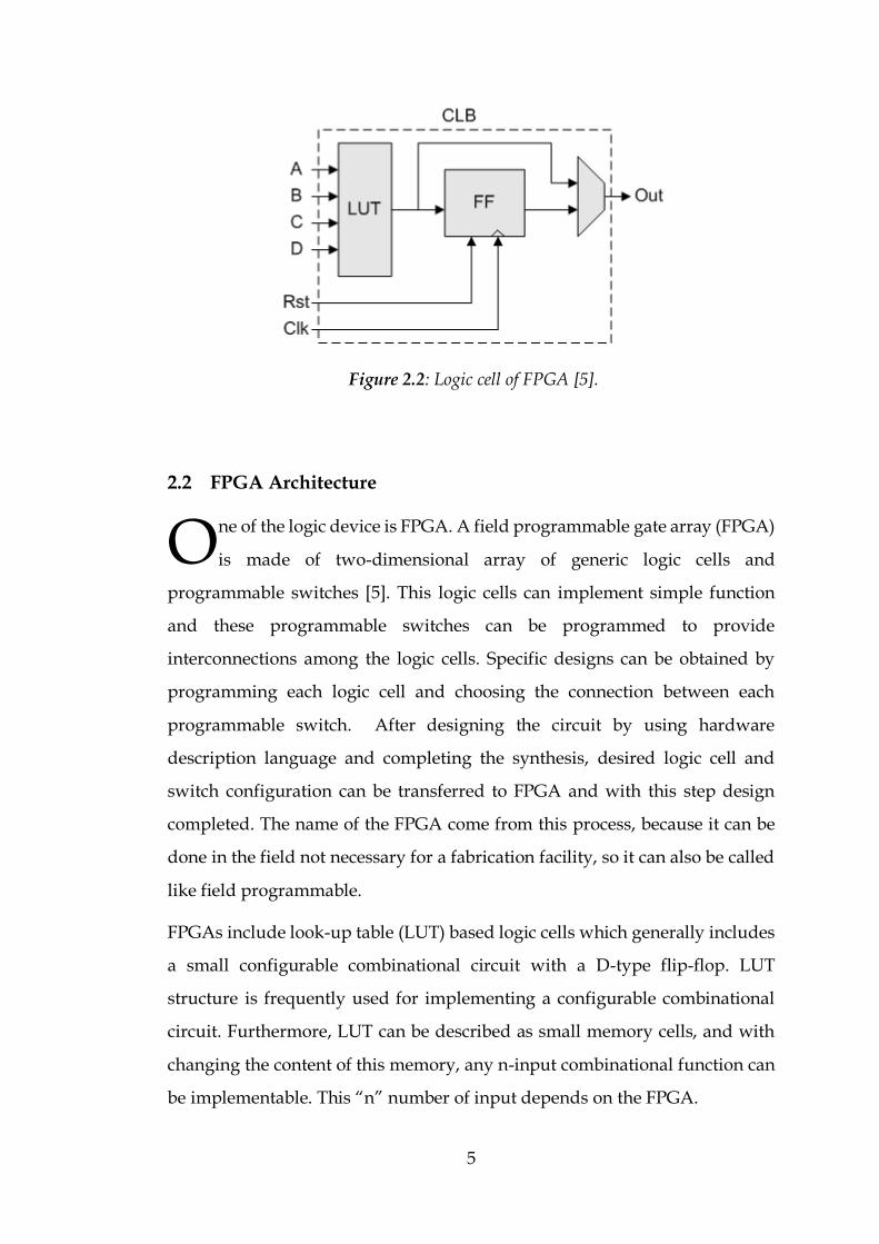
2.2 FPGA Architecture

ne of the logic device is FPGA. A field programmable gate array (FPGA)

is made of two-dimensional array of generic logic cells and

programmable switches [5]. This logic cells can implement simple function

and these programmable switches can be programmed to provide

interconnections among the logic cells. Specific designs can be obtained by

programming each logic cell and choosing the connection between each

programmable switch. After designing the circuit by using hardware

description language and completing the synthesis, desired logic cell and

switch configuration can be transferred to FPGA and with this step design

completed. The name of the FPGA come from this process, because it can be

done in the field not necessary for a fabrication facility, so it can also be called

like field programmable.

FPGAs include look-up table (LUT) based logic cells which generally includes

a small configurable combinational circuit with a D-type flip-flop. LUT

structure is frequently used for implementing a configurable combinational

circuit. Furthermore, LUT can be described as small memory cells, and with

changing the content of this memory, any n-input combinational function can

be implementable. This “n” number of input depends on the FPGA.

O

Figure 2.2: Logic cell of FPGA [5].

6

The other most embedded blocks on FPGA’s are macro cells. These macro cells

include clock management circuits, memory blocks, I/O interface circuits and

combinational multipliers.

2.3 Configuration

2.3.1 Languages

2.3.1.1 Verilog

erilog is one of the hardware language that used to describe a digital

system [6]. It is invented between 1983 and 1984 by Phil Moorby and

Prabhu Goel [7]. After 1985, it is changed as a hardware modelling language.

The first Verilog simulator was started to use in 1985 and it evolved with time.

Structure of Verilog is similar to C language because of this reason digital

system designers started to use this language frequently. Verilog language has

a case sensitive property like C language and some of its control flow

keywords shows same functionality. On the other hand, it includes some

different properties, in contrast the traditional programming languages,

V

Figure 2.3: FPGA Internal Structure [5].

7

Verilog does not execute the blocks sequentially, so Verilog is called as a

dataflow language. A Verilog design can be created by using hierarchy of

modules, which can communicate with each other through a set of alleged

input, output, and bidirectional ports. However, Verilog designer has to

consider that the blocks themselves are executed concurrently. If the designed

Verilog code includes synthesizable statements, Verilog source code can be

convertible to logically equivalent hardware components with the connections

between them.

2.3.1.2 VHDL

ery High Speed Integrated Circuit Hardware Description Language

(VHDL) is the other hardware description language to design and test

digital circuits. VHDL arose out by the United States Department of Defence

to describe the function and the structure of integrated circuits. This

programming language was started to use 1980’s and with development of

language, it involved in IEEE standards. VHDL is basically one of the parallel

programming language. Like Verilog, VHDL includes hierarchy of modules.

When VHDL used for systems design, it allows designers to observe the

behaviour of the designed system, and it can be described (modelled) and

verified (simulated) before synthesis tools translate the design into real

hardware (gates and wires).

V

8

2.3.1.3 High Level Synthesis

t first, until the 1960s, ICs were designed, optimized, and laid out by

hand in the hardware domain [8][9]. In the early 1970s, it was started to

use simulation at the gate level. By 1979, cycle-based simulation became

available. Later on place-and-route, schematic circuit capture, formal

verification, and static analysis introduced. After 1980s, Hardware Description

Languages (HDLs), such as Verilog and VHDL started to use widely. First

generation high-level synthesis (HLS) tools introduced during the 1990s.

High-level synthesis connects hardware and software domains; moreover, it

improves the productivity for hardware designers who can work at a higher

level of abstraction while creating high-performance hardware [11]. On the

other hand, software designers can accelerate the computationally intensive

parts of their algorithms on the FPGA. High-level synthesis design provides

A

Figure 2.4: High-level synthesis (HLS) design steps [10].

9

to develop algorithms and verify at the C-level. It also allows controlling the

C synthesis process through optimization directives.

High-level synthesis consists of scheduling, binding and control logic

extraction. These terms can be explained as:

Scheduling determines which operations occur during each clock cycle based

on: length of the clock cycle or clock frequency, time it takes for the operation

to complete, as defined by the target device and user-specified optimization

directives.

The speed of FPGA decides the number of operations complete in one clock

cycle. If the FPGA is faster more operations completed in one clock cycle, on

the other hand if the FPGA is slower, it will take more clock cycles to complete

the operation therefore multicycle resources are needed to be use.

Binding determines which hardware resource implements each scheduled

operation. High-level synthesis uses information about the target device to

implement the optimal solution.

Control logic extraction extracts the control logic to create a finite state

machine (FSM) that sequences the operations in the RTL design.

Nowadays, there are many vendors in use, and one of them is Bambu compiler

that is academic licensed by PoliMi (Politecnico di Milano). This compiler uses

C as an input and creates Verilog as an output.

2.4 Today’s FPGA

owadays, FPGAs mostly used for implementing parallel design

methodologies, because this kind of implementation is not possible in

dedicated DSP designs. Some ASIC design methods, which allows designer to

implement designs at gate level can be used for FPGA design. On the other

hand, designers frequently use hardware languages like Verilog or VHDL. The

reason of this usage is that hardware languages show similar properties to

software design therefore it is more convenient.

N

10

In the past, FPGAs are mostly used for lower speed, lower complexity and

lower volume designs, however today’s FPGAs easily push the 500MHz

performance barrier [12]. With the time, logic density of FPGAs have increased

and it gives rise to improve the features of embedded processors, DSP blocks,

clocking, and high-speed serial at ever lower price points.

11

3. ALGORITHM OVERVIEW

3.1 Background for Least Squares Method

efore starting discussion of different methods, it is useful to aware of

some conceptual terms to better understand the algorithms and further

processes. The basic problem is described as a parameter identification

problem. It is noticeable from the name that the main principle is to identify a

best estimate of the values of one or more parameters in a regression. Different

techniques and estimation models can be used to solve and describe this

problem. In this thesis, some of the proper methods are discussed and the

results of used algorithms are demonstrated.

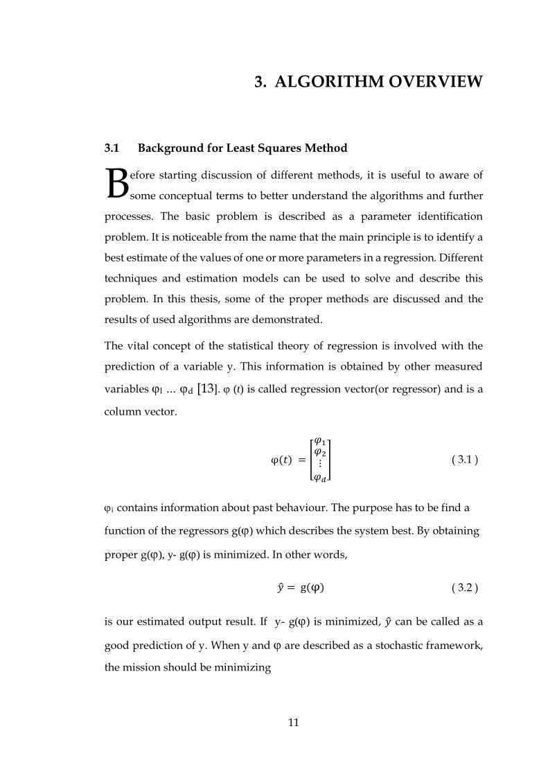
The vital concept of the statistical theory of regression is involved with the

prediction of a variable y. This information is obtained by other measured

variables d [13]. (t) is called regression vector(or regressor) and is a

column vector.

φ(𝑡) = [

𝜑1𝜑2

⋮𝜑𝑑

] ( 3.1 )

i contains information about past behaviour. The purpose has to be find a

function of the regressors g() which describes the system best. By obtaining

proper g(), y- g() is minimized. In other words,

�̂� = g(φ) ( 3.2 )

is our estimated output result. If y- g() is minimized, �̂� can be called as a

good prediction of y. When y and are described as a stochastic framework,

the mission should be minimizing

B

12

𝐸 [𝑦 − 𝑔(𝜑)]2 ( 3.3 )

By using g() and known d , the equation g() is obtained and also it can

be described as

g(𝜑) = 𝐸 [𝑦|𝜑)] ( 3.4 )

This is also known as the regression function or the regression of y on 𝜑.

3.2 Least Squares Method

he method of least squares is aim to minimize the squared differences

between observed data and their expected values [14]. By using this

technique, it estimates parameters. It is mainly parameter estimation of

estimated function by using input and output signals of the system. The block

diagram is shown in the figure. Input signal is defined as u(t), instead of (t),

just as a notation difference.

Generally, a definite priori information about the relationship between y(t)

and (t) is not given. Alternately, we have historic data which are related

values of y and y and can be expressed as a function of time or just the

T

Figure 3.1: Estimation of parameters of a mathematical model from time-series of the input variable and the output variable [14].

13

number, like a samples. With increasing number of measurement, we can

increase also the number of error calculation to make better estimation.

The definition of this method can be described as, sums of squares of

differences between the dependent variables of data points and (the most

suitable) curve should be minimum.

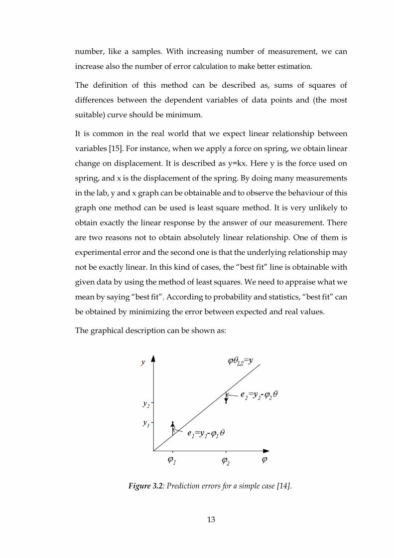
It is common in the real world that we expect linear relationship between

variables [15]. For instance, when we apply a force on spring, we obtain linear

change on displacement. It is described as y=kx. Here y is the force used on

spring, and x is the displacement of the spring. By doing many measurements

in the lab, y and x graph can be obtainable and to observe the behaviour of this

graph one method can be used is least square method. It is very unlikely to

obtain exactly the linear response by the answer of our measurement. There

are two reasons not to obtain absolutely linear relationship. One of them is

experimental error and the second one is that the underlying relationship may

not be exactly linear. In this kind of cases, the “best fit” line is obtainable with

given data by using the method of least squares. We need to appraise what we

mean by saying “best fit”. According to probability and statistics, “best fit” can

be obtained by minimizing the error between expected and real values.

The graphical description can be shown as:

Figure 3.2: Prediction errors for a simple case [14].

14

It will better describe with formulations.

With the historic data, we could replace the variance by the sample variance

as it is described before as a mission of algorithm.

1

𝑁∑[𝑦(𝑡) − 𝑔(φ(𝑡))]2𝑁

𝑡=1

( 3.5 )

By using linear regression

𝑔(φ) = 𝜃1φ1 + 𝜃2φ2 + ⋯+ 𝜃𝑑φ𝑑 ( 3.6 )

𝜃 is the parameters matrix which is built by the constant value of the expected

function.

𝜃 = [

𝜃1

𝜃2

⋮𝜃𝑑

] ( 3.7 )

Then it can be written as

𝑔(φ) = φ𝑇𝜃 ( 3.8 )

So when we combine linear regression formulas and the minimization formula

𝑉𝑁(𝜃) =

1

𝑁∑[𝑦(𝑡) − φ𝑇(𝑡)𝜃]2𝑁

𝑡=1

( 3.9 ) (3.9)

We need to obtain suitable 𝜃 to minimize 𝑉𝑁(𝜃) . And also, it can describe as

𝜃𝑁 = 𝑎𝑟𝑔𝑚𝑖𝑛 𝑉𝑁(𝜃) ( 3.10 )

φ𝑇𝜃𝑁 is used as predictor function and this method is called the least squares

estimate (LSE). When applied to historic data to algorithm, 𝜃𝑁 is mainly the

value that gives the best performing predictor. Minimization function is

quadratic function of 𝜃, therefore it can be minimized analytically.

15

[1

𝑁∑φ(𝑡)φ𝑇(𝑡)

𝑁

𝑡=1

] 𝜃𝑁 =1

𝑁∑φ(𝑡)𝑦(𝑡)

𝑁

𝑡=1

( 3.11 )

This set of equations is known as the normal equations. If the left side of

equation (∑ φ(𝑡)φ𝑇(𝑡)𝑁𝑡=1 ) is not singular which means invertible, we can

obtain LSE formula.

𝜃𝑁 = [1

𝑁∑φ(𝑡)φ𝑇(𝑡)

𝑁

𝑡=1

]

−1

1

𝑁∑φ(𝑡)𝑦(𝑡)

𝑁

𝑡=1

( 3.12 )

In general, the linear function can be described as y=ax+b, when we apply

linear estimation to least square estimate method

𝑆 = ∑[𝑦(𝑡) − (ax(t) + b)]2

𝑁

𝑡=1

( 3.13 )

The parameter matrix described as

𝜃 = [𝑎𝑏] ( 3.14 )

The regression matrix described as

φ(𝑡) = [𝑥(𝑡)1

] ( 3.15 )

To minimize S, derivative applied to find values of a and b. So

𝑑𝑠

𝑑𝑎= 0

𝑑𝑠

𝑑𝑏= 0 ( 3.16 )

𝑆 = ∑[𝑦(𝑡) − (ax(t) + b)]2

𝑁

𝑡=1

= ∑[(ax(t) + b) − 𝑦(𝑡)]2𝑁

𝑡=1

( 3.17 )

Partial derivative for a

16

𝑑𝑠

𝑑𝑎= 2∑[(ax(t) + b) − 𝑦(𝑡)]

𝑁

𝑡=1

x(t) = 0 ( 3.18 )

𝑑𝑠

𝑑𝑎= 𝑎 ∑[x(t)]2

𝑁

𝑡=1

+ 𝑏 ∑[x(t)]

𝑁

𝑡=1

− ∑[x(t)𝑦(𝑡)]

𝑁

𝑡=1

= 0 ( 3.19 )

Partial derivative for b

𝑑𝑠

𝑑𝑏= 2∑[(ax(t) + b) − 𝑦(𝑡)]

𝑁

𝑡=1

= 0 ( 3.20 )

𝑑𝑠

𝑑𝑏= 𝑎 ∑[x(t)]

𝑁

𝑡=1

+ 𝑏 ∑1

𝑁

𝑡=1

− ∑[𝑦(𝑡)]

𝑁

𝑡=1

= 0 ( 3.21 )

Describing these two equations in a matrix form

[ ∑[x(t)]2𝑁

𝑡=1

∑[x(t)]

𝑁

𝑡=1

∑[x(t)]

𝑁

𝑡=1

𝑁]

[𝑎𝑏] =

[ ∑[x(t)𝑦(𝑡)]

𝑁

𝑡=1

∑[𝑦(𝑡)]

𝑁

𝑡=1 ]

( 3.22 )

The Cramer Rule is applied to solve the matrix.

𝑎 =

|∑ [x(t)𝑦(𝑡)]𝑁

𝑡=1 ∑ [x(t)]𝑁𝑡=1

∑ [𝑦(𝑡)]𝑁𝑡=1 𝑁

|

|∑ [x(t)]2𝑁

𝑡=1 ∑ [x(t)]𝑁𝑡=1

∑ [x(t)]𝑁𝑡=1 𝑁

|

( 3.23 )

𝑎 =

𝑁 ∑ [x(t)𝑦(𝑡)] − ∑ [x(t)]∑ [𝑦(𝑡)]𝑁𝑡=1

𝑁𝑡=1

𝑁𝑡=1

𝑁 ∑ [x(t)]2𝑁𝑡=1 − ∑ [x(t)]𝑁

𝑡=1 ∑ [x(t)]𝑁𝑡=1

( 3.24 )

𝑏 =

|∑ [x(t)]2𝑁

𝑡=1 ∑ [x(t)𝑦(𝑡)]𝑁𝑡=1

∑ [x(t)]𝑁𝑡=1 ∑ [𝑦(𝑡)]𝑁

𝑡=1

|

|∑ [x(t)]2𝑁

𝑡=1 ∑ [x(t)]𝑁𝑡=1

∑ [x(t)]𝑁𝑡=1 𝑁

|

( 3.25 )

17

𝑏 =

∑ [x(t)]2𝑁𝑡=1 ∑ [𝑦(𝑡)]𝑁

𝑡=1 − ∑ [x(t)𝑦(𝑡)] ∑ [x(t)]𝑁𝑡=1

𝑁𝑡=1

𝑁 ∑ [x(t)]2𝑁𝑡=1 − ∑ [x(t)]𝑁

𝑡=1 ∑ [x(t)]𝑁𝑡=1

( 3.26 )

According to prediction function, estimated values of constants 𝜃 = [𝑎𝑏] can be

found by formulas which written above for linear least squares method.

To test our formulation, we can just consider 2 point and apply our algorithm.

Assuming our points are (x1,y1), (x2,y2). Calculation of slope(a) has to be:

𝑎 =

2((x1y1) + (x2y2)) − (x1 + x2)(y1 + y2)

2(x12 + x2

2) − (x1 + x2)2 ( 3.27 )

𝑎 =

2(x1y1) + 2(x2y2) − x1y1 − x1y2 − x2y1 − x2y2

2x12 + 2x2

2 − x12 − 2x1x2 − x2

2 ( 3.28 )

𝑎 =

(x1y1) + (x2y2) − x1y2 − x2y1

x12 + x2

2 − 2x1x2=

x1(y1 − y2) − x2(y1 − y2)

(x1 − x2)2 ( 3.29 )

𝑎 =

(x1 − x2)(y1 − y2)

(x1 − x2)2=

(y1 − y2)

(x1 − x2) ( 3.30 )

It can be seen above that algorithm gives the correct calculation of slope in

case of two points.

Least squares method is programmed by using C language. With given

samples, linear equation ( 3.31 ) is obtained by using LSE algorithm.

𝑦 = 15.569663 𝑥 + 59.487280 ( 3.31 )

By using MATLAB, obtained result is drawn on given samples. The result is

shown in Figure 3.3.

18

3.3 Recursive Least Squares Method

n many of today’s applications, we need a model that can work with online

data while the system is in operation.[3] The model includes the previous

information and with obtained new information, it changes its model

parameters to reduce the error between the real data and the estimated data.

There is need for this kind of systems, if the required result is obtained in real

time or it is required in order to take some decision about time with new

observed data. Methods that tries to solve this kind of problems or try to adjust

the system with an arrival of sequential data are usually called adaptive

systems.

I

Figure 3.3: Linear estimation of samples.

19

The method that used to compute modelling with online data is called

recursive identification methods, because the data are processed recursively

(sequentially) as they obtained. The other names to call this technique are real-

time identification or on-line identification.

We have already calculated the least squares estimator formula in equation

( 3.12 ). By using the equation in 3.12, recursive least square equation is

derivable. When we start from this equation

𝜃𝑁 = [1

𝑁∑φ(𝑡)φ𝑇(𝑡)

𝑁

𝑡=1

]

−1

1

𝑁∑φ(𝑡)𝑦(𝑡)

𝑁

𝑡=1

( 3.32 )

With new arriving data we can extend our first algorithm. The new data set

includes ⟨x𝑁+1, y𝑁+1⟩ and it is added to the training set.

Training set of N samples as:

𝜃𝑁 = [𝜑𝑁𝑇𝜑𝑁]−1𝜑𝑁

𝑇 𝑌𝑁 ( 3.33 )

Where the subscript (N) is added to denote the number of samples used for

the estimation. By using recursive least square method, the last value is added

to algorithm and the estimated model is obtainable. By using this method, we

do not need to use all N+1 available data to derive the equation.

SYSTEM

DECISION

MODEL

Figure 3.4: Adaptive methods.

20

By adding new data, the parameters are updated with the formula of ( 3.33 ).

New estimated matrix can be written as:

𝜃𝑁+1 = ([

𝜑𝑁

x𝑁+1]𝑇

[𝜑𝑁

x𝑁+1])

−1

[𝜑𝑁

x𝑁+1]𝑇

[𝑌𝑁

y𝑁+1] ( 3.34 )

By defining a new 𝑆𝑁matrix

𝑆𝑁+1 = (𝜑𝑁+1𝑇 𝜑𝑁+1) = [𝜑𝑁

𝑇 x𝑁+1𝑇 ] [

𝜑𝑁

x𝑁+1] ( 3.35 )

𝑆𝑁+1 = (𝜑𝑁𝑇 𝜑𝑁 + x𝑁+1

𝑇 x𝑁+1) = 𝑆𝑁 + x𝑁+1𝑇 x𝑁+1 ( 3.36 )

Since

[

𝜑𝑁

x𝑁+1]𝑇

[𝑌𝑁

y𝑁+1] = 𝜑𝑁

𝑇 . 𝑌𝑁 + x𝑁+1𝑇 y𝑁+1 ( 3.37 )

and

𝑆𝑁𝜃𝑁 = (𝜑𝑁𝑇 𝜑𝑁)[(𝜑𝑁

𝑇𝜑𝑁)−1𝜑𝑁𝑇 𝑌𝑁] = 𝜑𝑁

𝑇 𝑌𝑁 ( 3.38 )

We obtain

𝑆𝑁+1𝜃𝑁+1 = [

𝜑𝑁

x𝑁+1]𝑇

[𝑌𝑁

y𝑁+1] = 𝑆𝑁𝜃𝑁 + x𝑁+1

𝑇 y𝑁+1 ( 3.39 )

From the equation ( 3.39 ) 𝑆𝑁 is changed as:

𝑆𝑁+1𝜃𝑁+1 = (𝑆𝑁+1 − x𝑁+1𝑇 x𝑁+1)𝜃𝑁 + x𝑁+1

𝑇 y𝑁+1 ( 3.40 )

𝑆𝑁+1𝜃𝑁+1 = 𝑆𝑁+1𝜃𝑁 − x𝑁+1𝑇 x𝑁+1𝜃𝑁 + x𝑁+1

𝑇 y𝑁+1 ( 3.41 )

Or equivalently

𝜃𝑁+1 = 𝜃𝑁 + 𝑆𝑁+1−1 x𝑁+1

𝑇 (y𝑁+1 − x𝑁+1𝜃𝑁) ( 3.42 )

From the equations ( 3.36 ) and ( 3.42 ) the recursive formulation obtained as:

21

𝑆𝑁+1 = 𝑆𝑁 + x𝑁+1𝑇 x𝑁+1 ( 3.43 )

γ𝑁+1 = 𝑆𝑁+1−1 x𝑁+1

𝑇 ( 3.44 )

𝑒 = y𝑁+1 − x𝑁+1𝜃𝑁 ( 3.45 )

𝜃𝑁+1 = 𝜃𝑁 + γ𝑁+1𝑒 ( 3.46 )

In the calculation of 𝜃𝑁+1, the old value of the same constant 𝜃𝑁 has used and

also it depends on the γ𝑁+1 which includes 𝑆𝑁+1−1 . This operation is

computationaly costly so the matrix inversion lemma is used to reduce the cost

of this function.

Matrix inversion lemma:

F, H, G, K are matrices with suitable orders. F, H and (F+GHK) are invertible.

(F + GHK)−1 = F−1 − F−1𝐺(H−1 + 𝐾F−1𝐺)−1𝐾F−1 ( 3.47 )

Apply to

𝑆𝑁+1 = 𝑆𝑁 + x𝑁+1𝑇 x𝑁+1 ( 3.48 )

We have

(𝑆𝑁+1)−1 = (𝑆𝑁 + x𝑁+1

𝑇 x𝑁+1)−1 ( 3.49 )

Once defined

𝑉𝑁 = 𝑆(𝑁)−1 = (𝜑𝑁

𝑇𝜑𝑁)−1 ( 3.50 )

When the matrix inversion lemma is applied

VN+1 = VN − VNx𝑁+1𝑇 (I + x𝑁+1VNx𝑁+1

𝑇 )−1xN+1 VN ( 3.51 )

VN+1 = VN −

(VNx𝑁+1𝑇 xN+1 VN)

(I + x𝑁+1VNx𝑁+1𝑇 )

( 3.52 )

22

By using matrix inversion lemma, the inversion is eliminated from the final

equations and second recursive formulation is

VN+1 = VN −

(VNx𝑁+1𝑇 xN+1 VN)

(I + x𝑁+1VNx𝑁+1𝑇 )

( 3.53 )

γ𝑁+1 = VN+1x𝑁+1𝑇 ( 3.54 )

𝑒 = y𝑁+1 − x𝑁+1𝜃𝑁 ( 3.55 )

𝜃𝑁+1 = 𝜃𝑁 + γ𝑁+1𝑒 ( 3.56 )

In the implementation of algorithm in the c code, formula ( 3.57 ) and formula

( 3.58 ) is used.

𝑉𝑁 = 𝑉𝑁−1 −

𝑉𝑁−1. 𝜑𝑁 . 𝜑𝑁𝑇 . 𝑉𝑁−1

1 + 𝜑𝑁𝑇 . 𝑉𝑁−1 . 𝜑𝑁

( 3.57 )

𝜃𝑁 = 𝜃𝑁−1 + 𝑉𝑁 . 𝜑𝑁 [𝑦𝑁 − 𝜑𝑁𝑇 . 𝜃𝑁−1] ( 3.58 )

Formula ( 3.58 ) updates the estimates at each step based on the error between

the model output and the predicted output.

3.3.1 Linear Estimation

he linear estimation is the basic and the principal estimation in the

statistics. Before proceeding with a more complicated estimation, linear

estimation method is implemented. The linear function can be described as

y=ax+b, the aim is to obtain the parameter matrix described as

𝜃 = [𝑎𝑏] ( 3.59 )

The regression matrix described as

T

23

φ(𝑡) = [𝑥(𝑡)1

] ( 3.60 )

After we can use our recursive, least squares estimation algorithm

𝑉𝑁 = 𝑉𝑁−1 −

𝑉𝑁−1. 𝜑𝑁 . 𝜑𝑁𝑇 . 𝑉𝑁−1

1 + 𝜑𝑁𝑇 . 𝑉𝑁−1 . 𝜑𝑁

( 3.61 )

𝜃𝑁 = 𝜃𝑁−1 + 𝑉𝑁 . 𝜑𝑁 [𝑦𝑁 − 𝜑𝑁𝑇 . 𝜃𝑁−1] ( 3.62 )

For linear estimation, the matrix 𝑉0 has to be 2x2 and it is defined as

𝑉0 = [1 00 1

] ( 3.63 )

By reading example samples from the file “a” and “b” constants are obtained.

The graph is obtained by using 350 sample. Estimated linear function is

obtained and it is drawn on the samples.

24

3.3.2 Second Order Polynomial Estimation

here are other cases that linear estimation is not enough to describe the

behaviour of the system. In this kind of cases, higher order estimation

techniques are required to use to obtain the function that is better characterize

the function of our samples.

The second order polynomial estimation function can be described as:

𝑦 = 𝑎𝑥2 + bx + c , in this case, the equation has three unknown constants. This

matrix can be described as:

𝜃 = [

𝑎𝑏𝑐] ( 3.64 )

The regression matrix described as

φ(𝑡) = [

𝑥2(𝑡)

𝑥(𝑡)1

] ( 3.65 )

It can be also seen that the multiplication of these two vectors will give us our

function.

y = φ𝑇(𝑡)𝜃 ( 3.66 )

T

Figure 3.5: Linear estimation of samples by using RLS.

25

Now the recursive least squares estimation algorithm which is explained

before can be used.

Least squares estimation algorithm:

𝑉𝑁 = 𝑉𝑁−1 −

𝑉𝑁−1. 𝜑𝑁 . 𝜑𝑁𝑇 . 𝑉𝑁−1

1 + 𝜑𝑁𝑇 . 𝑉𝑁−1 . 𝜑𝑁

( 3.67 )

𝜃𝑁 = 𝜃𝑁−1 + 𝑉𝑁 . 𝜑𝑁 [𝑦𝑁 − 𝜑𝑁𝑇 . 𝜃𝑁−1] ( 3.68 )

For second order polynomial estimation, the matrix 𝑉0 has to be 3x3 and it is

defined as

𝑉0 = [

1 0 00 1 00 0 1

] ( 3.69 )

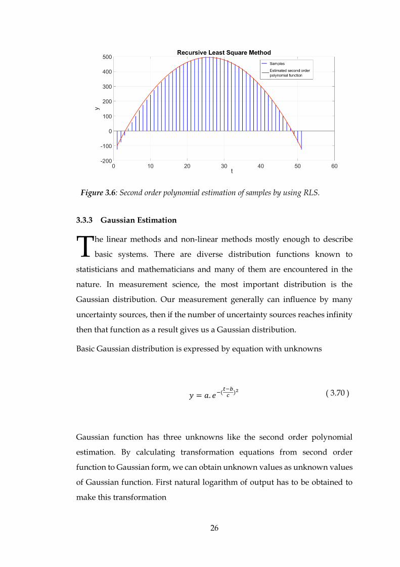
When the second order polynomial function is applied to recursive least

square method, the 𝜃 matrix can be obtained. Giving the samples in the

algorithm the second order function is obtained. The created samples and

estimated second order polynomial function on the samples are drawn in the

same graph. For each sample algorithm calculate new matrix of 𝜃. In the graph

shown, it can be seen all the samples and the last equation that is created by

the algorithm. The obtained equations show a graph determined, because all

the given samples are created by a determined function that does not fluctuate

at all.

The one has to be careful that with initial values and very limited input values,

it is possible not to reach deterministic value.

26

3.3.3 Gaussian Estimation

he linear methods and non-linear methods mostly enough to describe

basic systems. There are diverse distribution functions known to

statisticians and mathematicians and many of them are encountered in the

nature. In measurement science, the most important distribution is the

Gaussian distribution. Our measurement generally can influence by many

uncertainty sources, then if the number of uncertainty sources reaches infinity

then that function as a result gives us a Gaussian distribution.

Basic Gaussian distribution is expressed by equation with unknowns

𝑦 = 𝑎. 𝑒−(

𝑡−𝑏𝑐

)2 ( 3.70 )

Gaussian function has three unknowns like the second order polynomial

estimation. By calculating transformation equations from second order

function to Gaussian form, we can obtain unknown values as unknown values

of Gaussian function. First natural logarithm of output has to be obtained to

make this transformation

T

Figure 3.6: Second order polynomial estimation of samples by using RLS.

27

ln(𝑦) = ln(𝑎) − (

(𝑡 − 𝑏)

𝑐)

2

( 3.71 )

ln(𝑦) = −

𝑡2

𝑐2+

2 ∗ 𝑏 ∗ 𝑡

𝑐2−

𝑏2

𝑐2+ ln(𝑎) ( 3.72 )

Previously obtained equation is considered as:

ln(𝑦) = 𝛼 ∗ 𝑡2 + 𝛽 ∗ 𝑡 + 𝛾 ( 3.73 )

When we make them equal the previously obtained equation and the new

created equation by using Gaussian function.

𝛼 = −

1

𝑐2 ( 3.74 )

𝑐 = √−1

𝛼 ( 3.75 )

𝛽 =

2 ∗ 𝑏

𝑐2 ( 3.76 )

𝑏 =

𝑐2 ∗ 𝛽

2= −

1

𝛼∗

𝛽

2= −

𝛽

2 ∗ 𝛼 ( 3.77 )

𝛾 = −

𝑏2

𝑐2+ ln(𝑎) ( 3.78 )

28

ln(𝑎) = 𝛾 +

𝑏2

𝑐2 ( 3.79 )

𝑎 = 𝑒𝛾−

𝛽2

4∗𝛼 ( 3.80 )

We can obtain the transformation equations from second order function to

Gaussian function as:

[

𝛼𝛽𝛾] => [

𝑎𝑏𝑐] =

[ 𝑒𝛾−

𝛽2

4∗𝛼

−𝛽

2 ∗ 𝛼

√−1

𝛼 ]

( 3.81 )

To prove transformation equations by using example, the proper data set

(samples) is created. After using second order estimation and taking the

natural logarithm of “y” which is the value of histogram in this case, the

constant value of function obtained as:

[

𝛼𝛽𝛾] = [

−0.0304630.6040120.739675

] ( 3.82 )

When we use transformation equations to find “a”, “b” and “c” which are the

constants of Gaussian function. The constants obtained as:

[𝑎𝑏𝑐] = [

41.8333699.9137845.729439

] ( 3.83 )

The Gaussian function is obtained as:

𝑦 = 𝑎. 𝑒−(

𝑡−𝑏𝑐

)2 ( 3.84 )

29

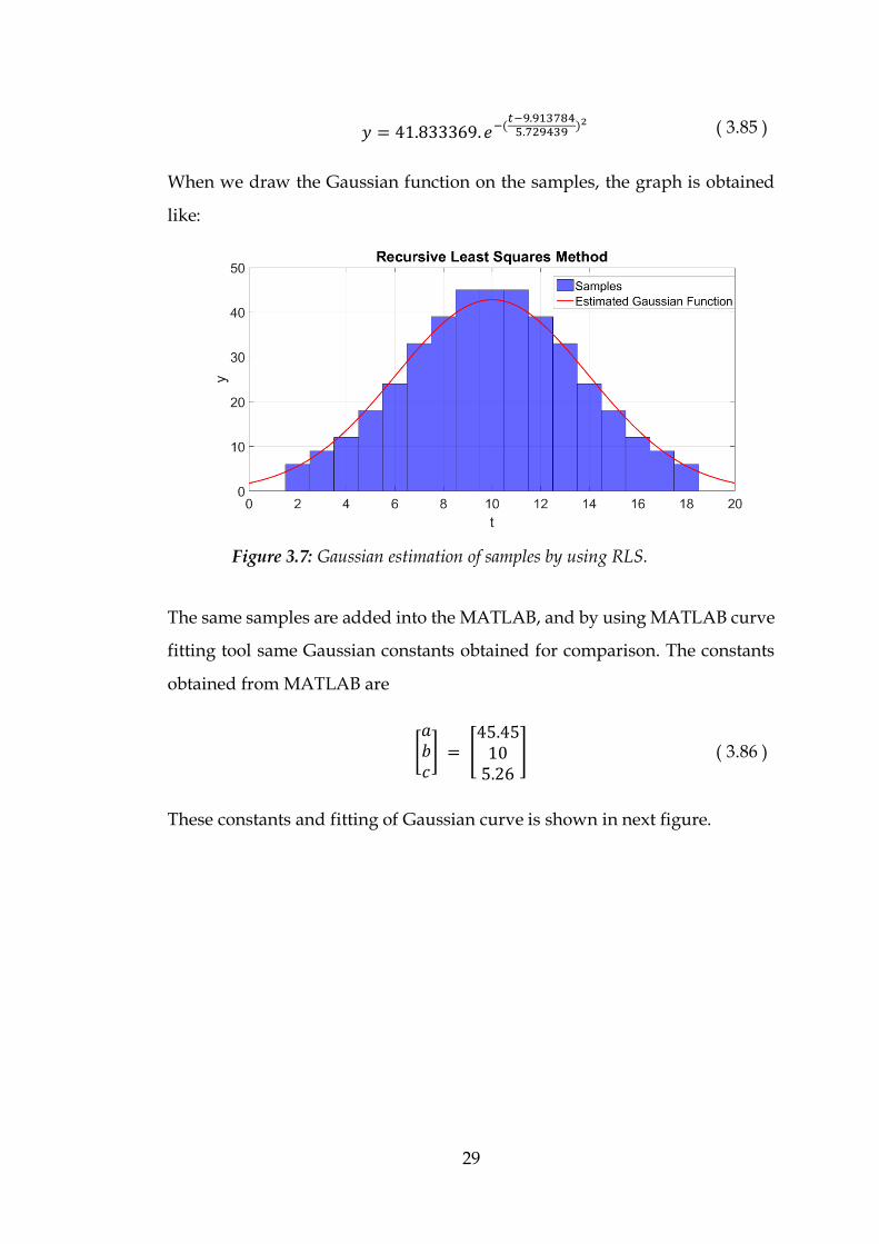
𝑦 = 41.833369. 𝑒−(𝑡−9.9137845.729439

)2 ( 3.85 )

When we draw the Gaussian function on the samples, the graph is obtained

like:

The same samples are added into the MATLAB, and by using MATLAB curve

fitting tool same Gaussian constants obtained for comparison. The constants

obtained from MATLAB are

[𝑎𝑏𝑐] = [

45.4510

5.26

] ( 3.86 )

These constants and fitting of Gaussian curve is shown in next figure.

Figure 3.7: Gaussian estimation of samples by using RLS.

30

There are some reasons to observe different fitting results. One of the main

contribution is initial value of RLS Gaussian fitting algorithm. With proper

chosen initial values, it is possible to reduce the error between fitting and the

real Gaussian function representation of the samples. The other one is, by

using recursive least squares algorithm actually the data is provided

sequentially to the algorithm, which means all the data set is not inserted

directly into the algorithm. Therefore, in contrast to MATLAB Gaussian fitting

computation, RLS Gaussian fitting cannot calculate and apply mean value of

data set and variance of data set.

Figure 3.8: MATLAB Gaussian Fitting.

Figure 3.9: Comparison of MATLAB Gaussian Fitting and RLS Gaussian Fitting.

31

3.4 Creation of Histogram

o use the data that created from the application that used in this thesis,

we need a conversion method. The measurement obtained from our

system can be collected in a specific windowing and by choosing the number

of measurement we obtain; we can create a histogram that shows the

characteristic of our measurement.

When we consider our real measurement, the data is the time measurement

and according to how many times we obtained this data, we will get a graph

that is predicted as a Gaussian behaviour.

To obtain this behaviour for observed time interval, we need to make time

division to obtain delta time that also can be considered as a resolution. For

next step, we need to count number of samples that are observed in this

specific delta time intervals. After enough amount of samples, the Gaussian

behaviour can be observable.

One example can be seen below:

T

Figure 3.10: Histogram creation example.

32

The time interval divided by 100 and 1000 samples observed. Gaussian

behaviour obtained from measurement as expected.

The crucial point here is that, by using recursive least squares algorithm, we

would like to obtain an equation that tries to best fit to obtained histogram and

when the number of sample increase as a conclusion all the values in N axis

will increase so we cannot obtain constant Gaussian profile. For instance, if we

think about second order polynomial this polynomial will show steeper

behaviour with increasing N values. It is shown arbitrarily in the next figure.

To obtain consistent graph, the solution is that we need to fix the number of

samples that used to create histogram. By using constant number of sample in

histogram, the estimated function’s constant parameters will obtained

decisively.

3.5 RLS Algorithm Implementation

o explain three different method, we can start with considering our

model is second order polynomial equation, for the Gaussian estimation

it is just the mathematical conversion of constant parameters. In this case 𝜃𝑁 is

a 3x1 matrix and it includes alpha, beta and gamma values.

T

Figure 3.11: Change of histogram.

N

t

33

θ̂N = [

αβγ] ( 3.87 )

To predicting our model as:

αt2 + βt + γ = y ( 3.88 )

Constants that we need to obtain:

α = alpha

β = beta

γ = gamma

Regression vector:

φ(𝑛) = [

𝑡2

𝑡1

] ( 3.89 )

“t” is the time measured by our system. Figure 3.12 shows the basic block

diagram of the algorithm.

34

3.5.1 1st Method

here are different ways to use recursive least squares algorithm. 1st

method is dividing data set in windows and create histogram from each

windows. By using these created histograms values, estimated functions

parameters are obtained. In this method, we do not need to keep the

information of previous histogram, because with coming new N sample, new

histogram is created. On the other hand, to obtain the new results it is

necessary to wait coming new N sample. Moreover, the obtained constants of

the equation are going to be independent from the one that calculated

previously.

T

Figure 3.12: Basic block diagram of the algorithm

35

The important notice to use this method is that N sample, which chosen to

create histogram and the division of the histogram plays important role to

reach a deterministic value. With wrong chosen N sample and histogram

division, it is possible to reach a result that is not the final regime. The other

coming samples will be used to create the other histogram and it will not affect

the first result ,so if the N sample and the histogram division are chosen the

same as previous ones and if it is not enough the reach a regime, the algorithm

cannot provide the final correct function. To solve this problem and to create

a system that can use the previous obtained constants, the 3rd method has to

be used.

3.5.2 2nd Method

he second method introduce new concept regarding to first method. By

using second method, it is not necessary to wait second N sample to

calculate the second result of recursive least square algorithm. After obtaining

T

Figure 3.13: Basic diagram of 1st method

36

first result with N sample, new coming sample is directly used and added into

the previous histogram. With addition of new coming value the number of

sample that used to create histogram will increase, therefore the first sample

that introduced to create the first histogram has to be eliminated from the

histogram. With addition of the new value and subtraction of the first value,

the new histogram is obtained. Now, this histogram can be used to obtain the

constant values of estimated function. This steps are shown in figure 3.14. Each

new sample is used to create new histogram. With new samples, steps are

repeating and these steps are described with different colours in the figure.

The advantage of this method compare the first one is that the system does not

need to stand by until reaching the new N sample to obtain the new result. It

is enough to get one more sample that means system will work consequently

with coming samples. On the other hand, the problem introduced in the first

method still not solved. Still, the obtained constants of the equation are going

Figure 3.14: Basic diagram of 2nd method

37

to be independent from the one that calculated previously, so it is important

to check used N sample and histogram division is enough to obtain expected

regime. Moreover, with this method, the array of N sample is introduced,

therefore it will consume space in memory in contrast the first method.

3.5.3 3rd Method

ddition to other methods, the previous 𝜃 matrix can be used to create

new 𝜃 which includes the constant values of the function. In this

method, N number of sample is decided to create histogram, the coming new

sample has to added to this histogram but the one has to be careful that this

new sample will increase the value in the histogram. If the other coming

samples are added like the previous one, the problem discussed in creation of

histogram will occur. Therefore, we need to fix N sample that is used to create

histogram. With coming new sample, the first element of the N sample array

has to be cancelled and the new histogram has to be created with a new coming

sample. With the cancelation of first element of the array, the other elements

has to shift and the second element has to take place of the first element,

therefore with a constant size of array, the algorithm can be implementable.

The size of array also an important factor because when we implement this

code on programmable gate array, it will locate in memory. It is preferred to

consume as less space as possible. This method is shown in the figure and the

difference between second method and this one is that there is a direct

connection between previous calculation and the new calculation. The new

constants that obtained from calculation are connect to the previous ones.

A

38

The main advantage of this method is that with each coming sample, RLS

algorithm used with an initial values of 𝜃 which is obtained previously. The

system shows progressive characteristic and it is not discrete calculation

anymore. The obtained constants of the equation are going to be dependent

from the one that calculated previously. If all the samples describe stable

function with chosen value of N sample for creation of histogram and proper

histogram division, with increasing number of sample inserted in algorithm,

the obtained function as a result will get close to steady regime.

3.6 Histogram Values

he creation of histogram plays an important role to observe the behaviour

of our measurement. There are some parameters to create the histogram.

These parameters are division of histogram, number of sample that used to

create histogram, minimum value and maximum value of created histogram.

T

Figure 3.15: Basic diagram of 3rd method

39

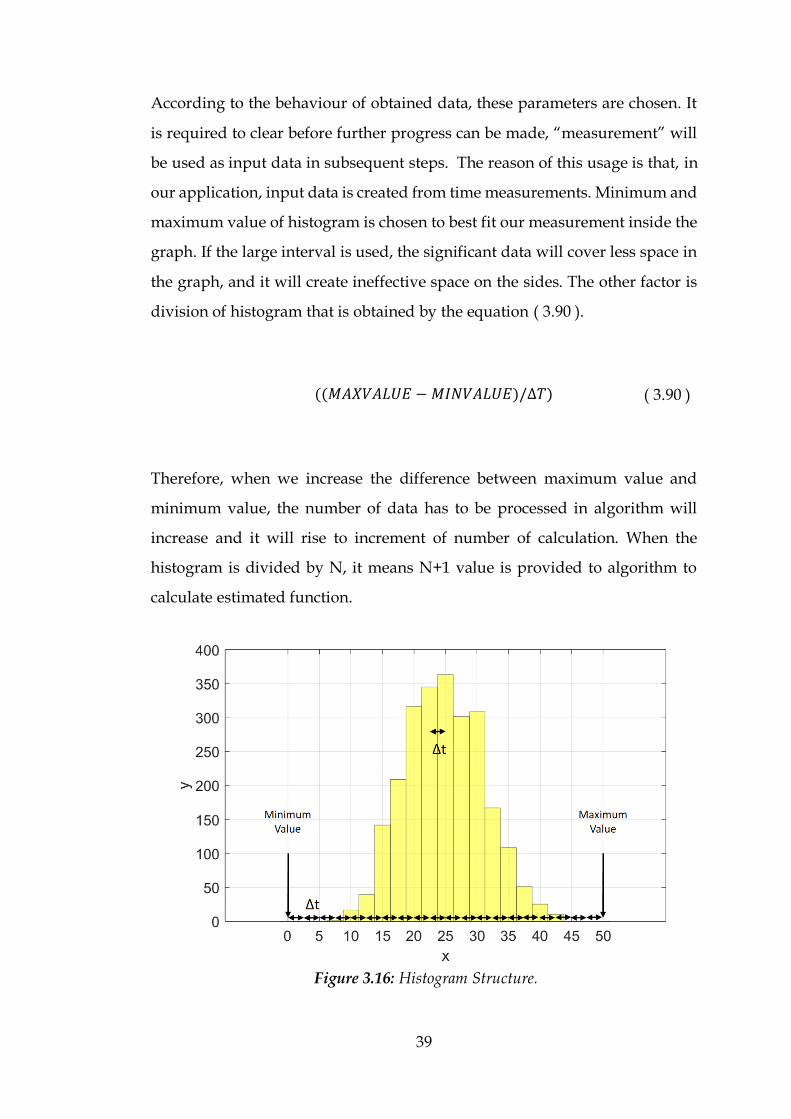
According to the behaviour of obtained data, these parameters are chosen. It

is required to clear before further progress can be made, “measurement” will

be used as input data in subsequent steps. The reason of this usage is that, in

our application, input data is created from time measurements. Minimum and

maximum value of histogram is chosen to best fit our measurement inside the

graph. If the large interval is used, the significant data will cover less space in

the graph, and it will create ineffective space on the sides. The other factor is

division of histogram that is obtained by the equation ( 3.90 ).

((𝑀𝐴𝑋𝑉𝐴𝐿𝑈𝐸 − 𝑀𝐼𝑁𝑉𝐴𝐿𝑈𝐸)/∆𝑇) ( 3.90 )

Therefore, when we increase the difference between maximum value and

minimum value, the number of data has to be processed in algorithm will

increase and it will rise to increment of number of calculation. When the

histogram is divided by N, it means N+1 value is provided to algorithm to

calculate estimated function.

Figure 3.16: Histogram Structure.

40

Figure 3.16 also shows the general structure of histogram. The figure has a

minimum limit of measurement 0, maximum limit of measurement 50. The

histogram is divided by 20, so it means that there are 20 intervals and we are

providing 20+1=21 value to algorithm including minimum and maximum

value.

Division of histogram, according to maximum and minimum value of

histogram, is used to choose delta time (∆𝑇). This parameter decides the

resolution of our histogram. It can be better seen in graphs that used different

number of division. In Figure 3.17, Figure 3.17, Figure 3.19 and Figure 3.20.

minimum value of graph is chosen 0 and maximum value of graph chosen 50.

Minimum and maximum values are fixed to show only the significance of

changing division.

The number of data that used the create algorithm will shape mainly the

amplitude of the histogram; however it has to be considered that less number

of measurement can provide unstable or insignificant results.

Figure 3.17: Histogram Divide by 10.

41

There is a specific number of measurement that is chosen and inserted in the

histogram. This technique also can be considered as windowing technique.

The measurement is obtained in the real time or the measurement is a set of

data and that number has to be chosen by considering limits of algorithm,

limits of equation and limits of precision. On the other hand, if there is a set of

data and putting this data in histogram then obtaining the prediction of graph

is not precise enough, the data set can be divided in the windows that is

mentioned as N sample. As indicated previously in chapter 3.5, different

methods can be used to obtain results that are more precise.

Figure 3.19: Histogram Divide by 50.

Figure 3.18: Histogram Divide by 100.

42

Increasing the number of sample is not an only criterion as outlined above.

Figure 3.20 shows clearly that decreasing Δ time can result crucial errors. If the

resolution of our measurement is lower than the chosen Δ time, it can provide

undesirable zero values.

All these parameters play an essential role and they have to be chosen

according to properties of measurement and properties of histogram that is

desired.

Figure 3.21 shows different division factors in one graph to create general idea

about histogram divisions.

Figure 3.20: Histogram Divide by 200.

43

3.7 C Interface

y using different techniques, algorithms and estimation methods, the

desired estimation can be obtained. As it mentioned above, at this point

choosing histogram and observing the obtaining results play a crucial role. To

bypass the MATLAB part and to observe the result in order to control the

accuracy of the result, C interface has been coded. By using this method, it is

now unnecessary to carry all the information to MATLAB and make analysis

on this data, furthermore we do not need to print the results and copy this

results to MATLAB and compare it with the carried information. Interface

includes all the algorithms that presented and it provides an estimation by

using them. In addition to this, another library is written to create visualization

to algorithms.

Draw library provides different type of visualisation techniques. Some of them

includes some pattern differences like the visualisation of first value. By using

this library, it is possible to print any kind of data: input data, linear equation,

second order equation and Gaussian equation. In addition, it is possible to

choose the number of x data as a variable.

B

Figure 3.21: Histogram with Different Divisions.

44

Provide a readable and convenient graphical representation, the

normalization of graph property is added. If the value is bigger than 100-1000-

10000… it will normalize to a value which is smaller than 100 and the factor is

going to be seen on the graph as a normalization factor. By using this

technique, visualisation of graph will not be problem and any kind of data can

be used.

The menu of interface includes all the functions and user can easily choose

proper function.

Figure 3.22: Menu of the interface.

45

Entering the number of the function will provide us the desired function. As

it can be seen in the figure, in any step it is possible to return the main menu

just entering the number zero “0”.

Firstly, demonstration of the interface will be done by using half Gaussian

because by using full Gaussian it is not totally possible to see the functionality

of linear estimations.

In the next step, function “2” which is linear estimation by using Least Squares

(LS) algorithm has chosen.

The linear estimation that best fits the given data has obtained. Function “3” is

chosen to draw the obtained equation.

In the next figure, the same data is processed and obtained the second linear

equation that best fits the given data but this time by using Recursive Least

Square Method (RLS).

Figure 3.23: Processed data.

46

Figure 3.24: Linear estimation (LS) and graph.

Figure 3.25: Linear estimation (RLS) and graph.

47

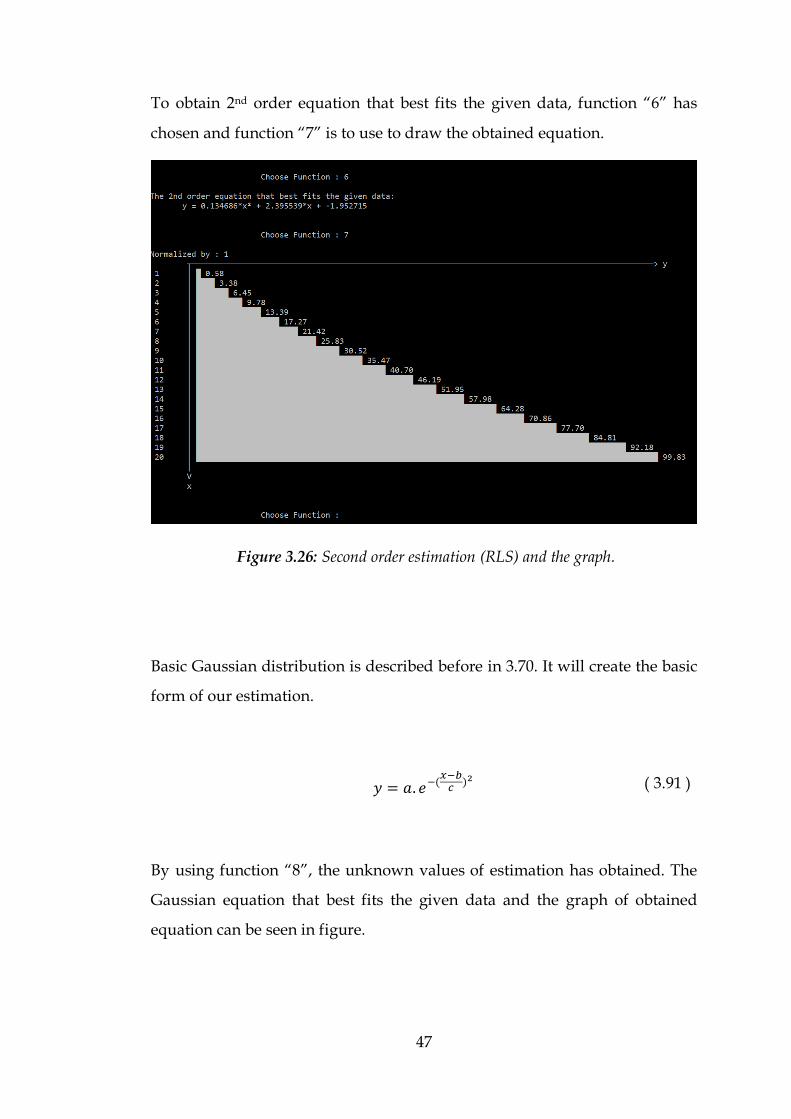
To obtain 2nd order equation that best fits the given data, function “6” has

chosen and function “7” is to use to draw the obtained equation.

Basic Gaussian distribution is described before in 3.70. It will create the basic

form of our estimation.

𝑦 = 𝑎. 𝑒−(

𝑥−𝑏𝑐

)2 ( 3.91 )

By using function “8”, the unknown values of estimation has obtained. The

Gaussian equation that best fits the given data and the graph of obtained

equation can be seen in figure.

Figure 3.26: Second order estimation (RLS) and the graph.

48

To show the Gaussian fitting truly, the full Gaussian data has added to the

program to investigate the estimated function. In the first graph, the used

Gaussian data has printed. The y value of the graph is exceeding the 100 so the

graph automatically normalized by 10 and normalization factor and

normalized values can be seen in the figure.

The estimated Gaussian function and the graph has obtained and shown in the

graph.

The program can be used in any kind of data and it provides the proper

estimation functions with their graph.

Figure 3.27: Gaussian estimation and the graph.

49

Figure 3.28: Graph of Gaussian data.

Figure 3.29: Estimation of Gaussian data and the graph.

50

3.8 Applications of Algorithms

he programme is designed general purpose which means by using

created algorithm, we can choose a model and we can find the unknown

parameters of the model. At the end, we will have estimated function with

known parameters. In addition, it is possible to draw the input data and the

final estimated model. Furthermore, we can compare the results visually. For

the input data, it is possible to use huge data sets. Also, it is possible to use big

values for the input data. In the system the number of precision can be

adjustable and default chosen precision is used up to 224. It is possible to

increase more and more but one need to be careful about the overflow of the

algorithm.

By using programmed algorithms, it is possible to calculate

Least Squares Method (LS)

o Linear Estimation

Recursive Least Squares Method (RLS)

o Linear Estimation

o Second Order Polynomial Estimation

o Gaussian Estimation

for the calculated histograms.

T

51

4. FPGA IMPLEMENTATION

4.1 PandA Project

andA project is aimed to develop an applicable framework that provides

HW-SW Co-Design field [16]. It includes methodologies supporting the

research on different areas. Such as: high level synthesis of hardware

accelerators, metrics for performance estimation of embedded software

applications, dynamic reconfigurable devices and hardware/software

partitioning and mapping.

PandA is a free software that developed at Politecnico di Milano. It is possible

to reach the latest version online as a downloadable content.

Bambu is a free framework that is used for the high level synthesis of complex

applications. It supports almost all the C constructs (e.g., function calls and

sharing of the modules, pointer arithmetic and dynamic resolution of memory

accesses, accesses to array and structs, parameter passing either by reference

or copy, …). Bambu is codded in C++ and it is developed for Linux systems.

It is available free under GPL license.

Bambu has a simple working principle. It receives as input a behavioral

description of the specification, written in C language, and generates the HDL

description of the corresponding RTL implementation as output. It is also

suitable with commercial RTL synthesis tools, along with a test bench for the

simulation and validation of the behaviour.

High level synthesis flow of Bambu quite similar to a software compilation

flow. It starts from a high level specification and creates low level code after a

sequence of analysis and optimization steps.

P

52

4.1.1 C Code Optimization for Bambu

he algorithm that will be used in the system has been chosen and

implemented in C. This algorithm has been tested on the created data set

and the estimated data set. After obtaining expected result, the same C code

has to be coded in an optimized way because it has to be considered that we

do not have infinite memory or infinite number of gates that can be used to

implement our C code. Designed C code has to be optimized as possible to

implement and occupy less space in the FGPA. In the subheadings, these

factors are explained.

4.1.1.1 Finite Precision Effects

ambu receives as input a behavioral description of the specification,

written in C language, and generates the HDL description of the

corresponding RTL implementation as output. Therefore, we need to consider

some properties of C that is not easy to implement HDL by using Bambu.

Scientific algorithm are generally developed in high level languages such as

MATLAB or C. Single or double precision floating point data structures are

used to support wide dynamic range while maintaining data precision.

Indeed, issues of truncation, rounding and overflows would seem frivolous at

a time where the validity of the algorithm is the absolute concern. On the other

hand, one can concern about the implementation in FPGA or ASIC, full

floating-point mathematics are often unsuitable. Floating-point operators

typically have dramatically increased logic utilization and power

consumption, combined with lower clock speed, longer pipelines, and

reduced throughput capabilities when compared to integer or fixed point.

Therefore, it is more logical to converting all or some of the algorithm to fixed

point, instead of just throwing more or larger logic devices at the problem. In

this point, it is important to understand the requirement and limitations. There

are two crucial argument, we need to consider algorithm adherence to

functional requirements and hardware adherence to design constraints.

T

B

53

4.1.1.1.1 Scale Factor Adjustment

he algorithm and the framework has been discussed and also considering

the information as it mentioned in previous section, floating point to

fixed point conversion (FFC) is completed. For the fixed-point conversion,

instead of power of ten, power of two is used to reduce the complication of the

system. By using fixing point, the algorithm implemented and expected results

are obtained. In the new code, all the variables are assigned to integer, in case

of requirement of big number of bit that cannot be handled in integer (16 bit),

long long integer, which is 64 bit is used.

4.1.1.1.2 Algorithm Modification with Scale Factor

mportance of scale factor plays important role in algorithm due to the usage

of fixed point. We need to consider our algorithm to use scaling factor. As

it mentioned before, two equation creates the concept of the algorithm.

𝑉𝑁 = 𝑉𝑁−1 −

𝑉𝑁−1. 𝜑𝑁 . 𝜑𝑁𝑇 . 𝑉𝑁−1

1 + 𝜑𝑁𝑇 . 𝑉𝑁−1 . 𝜑𝑁

( 4.1 )

𝜃𝑁 = 𝜃𝑁−1 + 𝑉𝑁 . 𝜑𝑁 [𝑦𝑁 − 𝜑𝑁𝑇 . 𝜃𝑁−1] ( 4.2 )

When we apply scaling to obtain fixed point, it will change as 4.3 and 4.4.

𝑉0 = [

1. 𝑃𝑟𝑒𝑐1 0 00 1. 𝑃𝑟𝑒𝑐1 00 0 1. 𝑃𝑟𝑒𝑐1

] ( 4.3 )

𝜃 = [

𝑎. 𝑃𝑟𝑒𝑐2𝑏. 𝑃𝑟𝑒𝑐2𝑐. 𝑃𝑟𝑒𝑐2

] ( 4.4 )

𝑉𝑁 = 𝑉𝑁−1 −

𝑉𝑁−1. 𝜑𝑁. 𝜑𝑁𝑇 . 𝑉𝑁−1

1 ∗ 𝑃𝑟𝑒𝑐1 + 𝜑𝑁𝑇 . 𝑉𝑁−1 . 𝜑𝑁

( 4.5 )

T

I

54

𝜃𝑁 = 𝜃𝑁−1 +𝑉𝑁 . 𝜑𝑁.

𝑃𝑟𝑒𝑐3𝑃𝑟𝑒𝑐1 [𝑦𝑁 . 𝑃𝑟𝑒𝑐2 − 𝜑𝑁

𝑇 . 𝜃𝑁−1]

𝑃𝑟𝑒𝑐3 ( 4.6 )

Scaling factors are chosen according to the values and importance of the

parameter. In most of the cases V matrix plays an crucial role. When the

algorithm runs V matrix elements takes the smallest value, therefore we need

to use high Prec1 value to avoid data loss.

Second function (4.6) includes additional factor, again this will compensate the

data loss. In addition to data loss, overflow factor has to be taken in account

when we use PrecX scaling factor. If it is possible to get overflow in one of the

calculation, it can cause irreparable error.

When the comparison is done between the precision usage and the float usage,

the difference arise because of the rounding. In the calculations the least

important bit will round in the float calculations. In case of precision, it case of

division it will directly cut that bit that does not depend on the following

value.

55

In the figure 4.1 the comparison between float and fixed point is shown. The

first value without parenthesis is the integer value multiplied with the

precision. Second value in the parenthesis is the same value divided by the

precision to see the real value and the compare with the float. The third line

Figure 4.1: Float and fixed point comparison.

56

with brackets is calculated by using float in the algorithm. There are small

differences between the obtained values but the crucial point is that usage of

data type must not affect the calculation of algorithm. If it creates overflow, it

can cause irreparable problems.

4.1.1.2 Optimization of Matrices

n coding process, the other critical factor is usage of memory. It has to be

considered that matrix calculations and memory management of matrices

are more complicated than one directional arrays or integer. The C code is

rewritten again to change 2-D arrays to 1-D (one directional) arrays. Instead of

using common matrix multiplication:

for (i = 0; i < 3; i++){

for (j = 0; j < 3; j++){

for (k = 0; k < 3; k++) {

mult[i][j] += multt[i][k] * V[k][j];

}

}

}

In the C code it is possible to see 3x3 matrix calculation as:

mult_1_1 = multt_1_1 * V[0] + multt_1_2 * V[3] + multt_1_3 * V[6];

mult_1_2 = multt_1_1 * V[1] + multt_1_2 * V[4] + multt_1_3 * V[7];

mult_1_3 = multt_1_1 * V[2] + multt_1_2 * V[5] + multt_1_3 * V[8];

mult_2_1 = multt_2_1 * V[0] + multt_2_2 * V[3] + multt_2_3 * V[6];

mult_2_2 = multt_2_1 * V[1] + multt_2_2 * V[4] + multt_2_3 * V[7];

mult_2_3 = multt_2_1 * V[2] + multt_2_2 * V[5] + multt_2_3 * V[8];

mult_3_1 = multt_3_1 * V[0] + multt_3_2 * V[3] + multt_3_3 * V[6];

I

57

mult_3_2 = multt_3_1 * V[1] + multt_3_2 * V[4] + multt_3_3 * V[7];

mult_3_3 = multt_3_1 * V[2] + multt_3_2 * V[5] + multt_3_3 * V[8];

This code seems ancient, however the tool can synthesis and optimize the C

code in an easier and more optimized way.

58

5. EXPERIMENTAL VALIDATION

5.1 Time to Digital Converter (TDC)

n many cases in science and industry accurate measurements of time

intervals (TIs) between two or more physical events are commonly needed

[17]. The basic example is that there are two electrical pulses that are obtained

or created by the source and these pulses are given to the device that can detect

the time difference between the leading edges of these pulses. Figure 5.1 shows

the basic principle. The time measurement is the difference between the

signals that entered START and STOP ports. TIM in the figure is time-interval

meter that measures the time interval between START and STOP. When the

TIM reads the time interval, it converts time into a digital (binary) word;

therefore, a TIM is also called a time-to-digital converter (TDC). Frequently

this name used for a short measuring range, usually shorter than 100ns to

200ns.

5.1.1 Measurement

he main property of multi-channel TDC is based on the use of a single

tapped-delay-line for all channels [18]. A tapped delay line (TDL) is a

delay line with taps. It can be seen in Figure 5.2 that there is a tap output that

I

T

Figure 5.1: Principle of TI measurement [18].

59

extracts a signal from somewhere within the delay line. In our measurement

technique, buffers are used for creating delay and between each buffer; there

is a tap to extract the signal.

As it mentioned before a time to digital converter with a tapped delay line

measures short time intervals. The resolution of this measurement is equal to

the delay of propagation between adjacent taps of the delay line. A nbit counter

clocked with period TCLK equal to the full-scale of the TDC is inserted to extend

the full-scale of measurable intervals. On this wise, a coarse estimation

(TCOARSE) that is performed by the counter and a fine contribution (TFINE) from

the TDC constitute the measurement.

Time measurement process is shown in Figure 5.3. The measurement of the

time interval shown with Tij and this measurement obtained by the formula of

( 5.1 ).

𝑇𝑖𝑗 = 𝑇𝑖𝑗𝐶𝑂𝐴𝑅𝑆𝐸 + 𝑇𝑖𝑗

𝐹𝐼𝑁𝐸 ( 5.1 )

Figure 5.2: Schematic representation of a TDL- TDC [18].

60

Clock signal is not synchronous with neither start event nor stop event,

therefore after calculating the 𝑇𝑖𝑗𝐶𝑂𝐴𝑅𝑆𝐸 , 𝑇𝑖𝑗

𝐹𝐼𝑁𝐸 is added to obtain correct

measurement. 𝑇𝑖𝑗𝐹𝐼𝑁𝐸 is the difference between 𝑇𝑖

𝐹𝐼𝑁𝐸 and 𝑇𝑗𝐹𝐼𝑁𝐸 as shown in (

5.2 ).

𝑇𝑖𝑗𝐹𝐼𝑁𝐸 = (𝑇𝑖

𝐹𝐼𝑁𝐸 − 𝑇𝑗𝐹𝐼𝑁𝐸) ( 5.2 )

Coarse measurement is created by number of clock period multiplied by the

clock period. On the other hand, this measurement obtained between the next

rising edge after the event[i] signal arrives and the next rising edge after the

event[j] arrives.

𝑇𝑖𝑗𝐶𝑂𝐴𝑅𝑆𝐸 = 𝑇𝐶𝐿𝐾 ∙ 𝑁𝑖𝑗

𝐶𝑂𝐴𝑅𝑆𝐸 ( 5.3 )

𝑁𝑖𝑗𝐶𝑂𝐴𝑅𝑆𝐸 = {

𝑁𝐽 − 𝑁𝑖 𝑁𝑗 ≥ 𝑁𝑖

2𝑛𝑏𝑖𝑡 + 𝑁𝐽 − 𝑁𝑖 𝑁𝑗 < 𝑁𝑖 ( 5.4 )

Figure 5.3: Time diagram of the measurement process [19].

61

When we combine the formulas, the final formula is obtained as a formula

( 5.5 ).

𝑇𝑖𝑗 = 𝑇𝐶𝐿𝐾 ∙ 𝑁𝑖𝑗𝐶𝑂𝐴𝑅𝑆𝐸 + (𝑇𝑖

𝐹𝐼𝑁𝐸 − 𝑇𝑗𝐹𝐼𝑁𝐸)

( 5.5 )

Time-to-digital converters (TDC) are very appropriate to be implemented into

FPGA devices. The advantageous are less production costs, minimum time-to-

market and great design flexibility.

The output measurement is obtained as Gaussian distribution due to the noise

contribution.

5.1.2 Characteristics of the Data

s it mentioned in previous chapters, observing characteristics and

choosing histogram division , minimum and maximum values are

playing a crucial role because these values will create the data set that the

algorithm work on. In the chapter 3.7, the new designed C interface that can

calculate the estimation and draw any kind of estimated function is

introduced. On the other hand, to choose proper values for minimum,

maximum or histogram division, we need an analysis of data that can be

obtained by MATLAB. The graphical interface is coded and explained, in

addition to the graphical interface to bypass again the MATLAB part, another

C interface is written. This interface can take minimum, maximum and

histogram division as an input and it can create the same results that MATLAB

creates. By using this new C design, we do not need to move our input data to

A

62

MATLAB and start investigating the graphs. It has a user friendly and clear

interface that can be seen in figure 5.4.

User interface asks in order of minimum value, maximum value and

histogram division. After entering proper parameters, we will obtain the same

result as MATLAB provides. The results of histogram creator is shown in

figure 5.5.

Figure 5.4: Histogram Creator Interface.

63

After adding the same data set to the MATLAB, the same histogram can be

obtained in the MATLAB by using:

histogram(VarName1,20,'BinLimits',[1400,1700]);

comment line.

Figure 5.6: MATLAB Histogram results.

Figure 5.5: Histogram Creator results.

64

It can be seen in the figures that the result of C code and the result of the

MATLAB is identical. Normalized factor can be seen as 1000 in the C interface.

In case of different demands on visualization of histogram, it is easy to change

visualization parameters. For instance, instead of two number in the fractional

part, it can change as the user want. Furthermore, it is possible to add

suggestion of minimum and maximum values, if the user knows the sigma

and the distribution of the Gaussian model. By adding average algorithm and

using the sigma, it is possible to estimate the minimum and maximum values

and suggest to user in the same interface.

5.1.3 Gaussian Estimation of the Data

he data is processed, minimum and maximum points are chosen and

histogram is divided to 20. RLS algorithm is applied and 4500 is chosen

as the number of data to create the histogram. 4500 is not a crucial number it

can be chosen as it is described in previous chapters. For very wide range of

data set the algorithm works without problem. 3rd method is chosen for the

calculation. The main advantage of this method is that with each coming

sample, RLS algorithm used with an initial values of 𝜃 which is obtained

previously. The system shows progressive characteristic and it is not discrete

calculation anymore. The obtained constants of the equation are going to be

dependent from the one that calculated previously. Information that is more

detailed can be found in chapter 3.5.3.

T

65

The algorithm is run for 100000 data and it most of the time remains in with

95% confidence bounds of MATLAB. This interval indicates that you have a

95% chance that the new observation is actually contained within the lower

and upper prediction bounds. Even though it goes out of 95% confidence

bounds, it does not diverge and return inside of confidence bounds. These

values are obtained from curve fitting tool of MATLAB. The values can be seen

in figure 5.7.

The values of C code can be seen in figure 5.8.

Figure 5.7: Curve Fitting Tool results.

66

In every step, one more data is taken from the data set and used to create a

new histogram. After obtaining new histogram, RLS algorithm obtains the

best fitting Gaussian equation.

MATLAB Code:

x = linspace(0,20,200);

%C Code Estimation

y = 584.381714.*exp(-((x-8.862715)/4.164752).*((x-8.862715)/4.164752));

hold on

plot(x,y,'b')

Figure 5.8: C code results.

67

%MATLAB Estimation

y = 605.5.*exp(-((x-8.804)/4.219).*((x-8.804)/4.219));

hold on

plot(x,y,'r')

bar(x21,VarName3,'FaceColor','y','FaceAlpha',.3,'EdgeAlpha',.3)

Graphs and calculations on C:

Figure 5.9: MATLAB Histogram results.

Figure 5.10: Data Set graph.

68

Figure 5.11: Estimated Gaussian Graph.

69

6. RESULTS

ith the time, the number of data that have been processed and created

from different applications show a massive increment. Considering

this growth, it became essential to create algorithms to analyse the obtained

data and to use estimation methods to predict the form of the data.

A key challenge in computational modelling is the determination of model

parameters. Generally, only a fraction of the parameters is experimentally

measured, the others have to be fitted according to the suggested model,

which uses fixed number of data. On the other hand, in many of today’s

applications, we need a model that can work with online data while the system

is in operation [3]. The model includes the previous information and it changes

its model parameters with obtained new information to reduce the error

between the real data and the estimated data. There is need for this kind of

systems, if the required result is obtained in real time and also if it is needed

to take some decision with new observed data.

Under consideration of above mentioned facts, different kind of algorithms

coded by using C language. These algorithms are tested on the ideal and the

real data sets. Furthermore, general-purpose estimation interface is designed

to use for any kind of data and it includes various estimation options. The user

can easily choose one or more of the option depending on the application. As

a case study, Time to Digital Converter has been chosen. The measured data

from time to digital converter are processed in designed C code and they are

used to create a histogram. The histogram is obtained to create the graph data

set that will be processed in coded RLS algorithm in C. According to the

obtained graph, Gaussian model is found as a fitting curve. Gaussian recursive

least square method has been used to obtain the unknown parameters of the

Gaussian equation. Same data processed in MATLAB and same histogram

W

70

data are given to the curve fitting tool of MATLAB. Gaussian form has been

chosen as a model and the model parameters are obtained. MATLAB results

and the results obtained from Gaussian recursive least square method

designed in C are compared. This comparison verified the correctness of the

results obtained in C.

Compared to Least Squares (LS) algorithms, recursive least squares (RLS)

algorithms have a faster convergence speed. However, RLS algorithms

involve more complicated mathematical operations and require more

computational resources than LS algorithms.

71

7. CONCLUSION AND FUTURE STUDIES

eneral-purpose estimation interface is designed to use for any kind of

data and it includes various estimation options. User can easily choose

one or more of the options depending on the application.

Different algorithms are designed in C

o Least Squares Method (LS)

o Recursive Least Squares Method (RLS)

Linear Estimation

Second Order Polynomial Estimation

Gaussian Estimation

RLS algorithm is used to create continuous parameters estimation

Various models are designed to create general purpose interface

Histogram Creator is designed to easily analyse different histograms

General purpose C library is coded to draw the graphs

User friendly interface is programmed

Results are compared and verified with MATLAB

The C code is also converted to Verilog code by using Bambu tool that is

provided by Politecnico di Milano in Linux. For the future study, a

communication interface can be provided between the output of the TDC and

the created Verilog algorithm. To achieve this, firstly, the obtained

measurement can be recorded to a block memory. While running algorithm

on this memory, new coming data can be recorded on the other memory. The

process will change when the process on one block memory is completed. In

addition, it is possible to understand the speed of the measurement and to

compare it with the working algorithm. Using some limitations, these

calculations can be synchronized. Another way is to stop or to over process

G

72

the fast running one, regardless, the measurement will come in a Gaussian

form. Missing some samples will not affect the running algorithm. At the end

the algorithm will provide the proper parameters of the estimated model.

73

8. References

[1] Lehmann, E.L., Casella, G., 1998. Theory of Point Estimation (New York:

Springer) pp 1–590

[2] Bhatia, A., Behl, A., Puri, A., 2015. “PLD Architecture and Application,”

International Journal of Innovative Research in Technology, volume 1, issue

12

[3] Andres, K., 1970. A Texas Instruments Application Report: MOS

programmable logic arrays. Texas Instruments. Bulletin CA-158. Report

introduces the TMS2000 and TMS2200 series of mask programmable PLAs.

[4] Petrone, J.G., Foo, S.Y., 2004. Adaptive Filter Architectures for FPGA

Implementation, The Florida State University College of Engineering.

[5] Chu, Pong P., 2008. FPGA Prototyping by VHDL Examples. Wiley-

Interscience, New Jersey.

[6] Tala, D.K., Verilog tutorial. http://www.asic-world.com, accessed on:

2016.06.28.

[7] Erdin, C., Ors, S.B., 2014. Design and Implementation of a Secure RFID

Systems and Tests.

[8] Knapp, D.W., 1996 Behavioral Synthesis: Digital System Design Using the

Synopsys Behavioral Compiler, Prentice Hall.

[9] Elliot, J.P., 1999. Understanding Behavioral Synthesis: A Practical Guide to

High-Level Design, Kluwer Academic Publishers.

[10] Coussy,P., Gajski, D.D.,Meredith, M., Takach, A., 2009. "An Introduction

to High-Level Synthesis," in IEEE Design & Test of Computers, vol. 26, no. 4, pp.

8-17.

[11] Xilinx, 2014. Vivado Design Suite User Guide.

74

[12] Xilinx, FPGA vs. ASIC. http://www.xilinx.com/fpga/asic.htm, accessed

on: 2016.06.15.

[13] Ljung, L., 1999. System Identification: Theory for the user, Prentice Hall

PTR, New Jersey, second edition.

[14] Haugen, F., 2010. Advanced Dynamics and Control, TechTeach.

[15] Miller, J.S., 2006. The Method of Least Squares, Brown University

[16] Panda about. http://panda.dei.polimi.it/, accessed on: 2016.10.15.

[17] Kalisz, J., 2004, "Review of methods for time interval measurements with

picosecond resolution", Metrologia (Instutute of Physics Publishing) 41 (1): 17–

32

[18] Lusardi, N., Geraci, A., 2015. Implementazione di un’architettura TDC

single-chain multicanale in dispositivi FPGA.

[19] Lusardi, N., Geraci, A., 2015. "8-Channels high-resolution TDC in

FPGA," 2015 IEEE Nuclear Science Symposium and Medical Imaging Conference

(NSS/MIC), San Diego, CA, pp. 1-2.

75

INDEX OF FIGURES

FIGURE 2.1: PLA STRUCTURE. [4] ............................................................................................................. 4

FIGURE 2.2: LOGIC CELL OF FPGA [5]. ....................................................................................................... 5

FİGURE 2.3: FPGA INTERNAL STRUCTURE [5]. ............................................................................................. 6

FIGURE 2.4: HIGH-LEVEL SYNTHESIS (HLS) DESIGN STEPS [10]. ........................................................................ 8

FİGURE 3.1: ESTİMATİON OF PARAMETERS OF A MATHEMATİCAL MODEL FROM TİME-SERİES OF THE İNPUT VARİABLE AND

THE OUTPUT VARİABLE [14]. ......................................................................................................... 12

FİGURE 3.2: PREDICTION ERRORS FOR A SIMPLE CASE [14]. ........................................................................... 13

FİGURE 3.3: LİNEAR ESTİMATİON OF SAMPLES. ........................................................................................... 18

FİGURE 3.4: ADAPTİVE METHODS............................................................................................................ 19

FİGURE 3.5: LINEAR ESTIMATION OF SAMPLES BY USING RLS. ........................................................................ 24

FİGURE 3.6: SECOND ORDER POLYNOMIAL ESTIMATION OF SAMPLES BY USING RLS. ............................................ 26

FİGURE 3.7: GAUSSIAN ESTIMATION OF SAMPLES BY USING RLS. .................................................................... 29

FİGURE 3.8: MATLAB GAUSSIAN FITTING. ............................................................................................... 30

FİGURE 3.9: COMPARISON OF MATLAB GAUSSIAN FITTING AND RLS GAUSSIAN FITTING. ................................... 30

FİGURE 3.10: HISTOGRAM CREATION EXAMPLE. ......................................................................................... 31

FİGURE 3.11: CHANGE OF HISTOGRAM. .................................................................................................... 32

FİGURE 3.12: BASIC BLOCK DIAGRAM OF THE ALGORITHM ............................................................................. 34

FİGURE 3.13: BASIC DIAGRAM OF 1ST METHOD ........................................................................................... 35

FİGURE 3.14: BASIC DIAGRAM OF 2ND METHOD .......................................................................................... 36

FİGURE 3.15: BASIC DIAGRAM OF 3RD METHOD .......................................................................................... 38

FİGURE 3.16: HISTOGRAM STRUCTURE. ................................................................................................... 39

FİGURE 3.17: HISTOGRAM DIVIDE BY 10. ................................................................................................. 40

FİGURE 3.19: HISTOGRAM DIVIDE BY 100. ............................................................................................... 41

FİGURE 3.18: HISTOGRAM DIVIDE BY 50. ................................................................................................. 41

FİGURE 3.20: HISTOGRAM DIVIDE BY 200. ............................................................................................... 42

FİGURE 3.21: HISTOGRAM WITH DIFFERENT DIVISIONS. ............................................................................... 43

FİGURE 3.22: MENU OF THE INTERFACE. .................................................................................................. 44

FİGURE 3.23: PROCESSED DATA. ............................................................................................................ 45

FİGURE 3.24: LINEAR ESTIMATION (LS) AND GRAPH. ................................................................................... 46

FİGURE 3.25: LINEAR ESTIMATION (RLS) AND GRAPH. ................................................................................. 46

FİGURE 3.26: SECOND ORDER ESTIMATION (RLS) AND THE GRAPH. ................................................................. 47

FİGURE 3.27: GAUSSIAN ESTIMATION AND THE GRAPH. ................................................................................ 48

FİGURE 3.28: GRAPH OF GAUSSIAN DATA. ................................................................................................ 49

FİGURE 3.29: ESTIMATION OF GAUSSIAN DATA AND THE GRAPH. .................................................................... 49

76

FIGURE 4.1: FLOAT AND FIXED POINT COMPARISON. .................................................................................... 55

FIGURE 5.1: PRINCIPLE OF TI MEASUREMENT [18]. ..................................................................................... 58

FIGURE 5.2: SCHEMATIC REPRESENTATION OF A TDL- TDC [18]. ................................................................... 59

FIGURE 5.3: TIME DIAGRAM OF THE MEASUREMENT PROCESS [19]. ................................................................ 60

FIGURE 5.4: HISTOGRAM CREATOR INTERFACE. .......................................................................................... 62

FIGURE 5.5: HISTOGRAM CREATOR RESULTS. ............................................................................................. 63

FIGURE 5.6: MATLAB HISTOGRAM RESULTS. ............................................................................................ 63

FIGURE 5.7: CURVE FITTING TOOL RESULTS. .............................................................................................. 65

FIGURE 5.8: C CODE RESULTS. ................................................................................................................ 66

FIGURE 5.9: MATLAB HISTOGRAM RESULTS. ............................................................................................ 67

FIGURE 5.10: DATA SET GRAPH. ............................................................................................................. 67

FIGURE 5.11: ESTIMATED GAUSSIAN GRAPH. ............................................................................................ 68

77