Optimal Design of Bridges for High-Speed Trains - DiVA …430650/FULLTEXT01.pdf · Optimal Design...
108
Optimal Design of Bridges for High-Speed Trains Single and double-span bridges CARINE MELLIER Master of Science Thesis Stockholm, Sweden 2010
Transcript of Optimal Design of Bridges for High-Speed Trains - DiVA …430650/FULLTEXT01.pdf · Optimal Design...

i
Optimal Design of Bridges for High-Speed Trains
Single and double-span bridges
CARINE MELLIER
Master of Science Thesis Stockholm, Sweden 2010


Optimal Design of Bridges for High-Speed trains
Single and double-span bridges
Carine Mellier
June 2010 TRITA-BKN. Master Thesis 301, 2010 ISSN 1103-4297 ISRN KTH/BKN/EX-301-SE

© Carine Mellier, 2010 Royal Institute of Technology (KTH) Department of Civil and Architectural Engineering Division of Structural Design and Bridges Stockholm, Sweden, 2010

i
Preface
This master thesis was carried out at the division of Structural Design and Bridges, at the Royal Institute of Technology (KTH) in Stockholm. The work was conducted under the supervision of Prof. Raid Karoumi to whom I want to thank for his advice, guidance, and for always having taken the time to discuss with me when I needed it. I also wish to thank Christoffer Johansson who arrived at the right moment to re-give me faith in the utility of my work, but also for his help, his advice, for reviewing this report and for the thousands of ideas he has in a day. I would like to thank Martin Mikus and Joakim Wallin who helped me to get familiar with ABAQUS, and also Mahir Ülker Kaustell who always found time to help me, to answer my questions and discuss with me. Finally, I would like to thank Ilkka Mansikkamäki for his support and his great help with MATLAB.
Stockholm, June 2010
Carine Mellier


iii
Abstract
To deal with an increasing demand in transportation, trains are made longer and faster. Higher speeds imply higher impacts on bridges. Therefore, structures have to be designed to resist these new constraints. The Eurocode (2002) introduced additional checks for the design of high-speed railway bridges. Among them, the maximum vertical deck acceleration criterion often determines alone the design of the structure. Tests on shake table brought to the conclusion that vertical bridge deck acceleration should never exceed 3.5 m/s2 for ballasted tracks.
This master thesis investigates the optimization of cross section parameters of single-track simply supported and double-span bridges based on the limit of the maximum vertical deck acceleration criterion. The first natural frequency is considered as a proof of the feasibility of the structure. The optimization is carried out through MATLAB for both types of bridges. The deck acceleration of simply supported bridges is analytically calculated using the Train Signature (ERRI D214 1999) in MATLAB. The dynamic calculations of double-span bridges are implemented through the finite element software ABAQUS. The implemented programs have been verified by comparison to values of simple cases found in the literature. Structures are tested under the influence of the ten HSLM-A trains of the Eurocode running at speeds between 150 km/h and 350 km/h.
Optimization algorithms are presented and compared in this study but their applicability in such context is questioned. Indeed, as the problem contains several suitable minima, the algorithms, which end in one solution, are not adapted. To overtake this difficulty, a scanning of the interesting zone is advised. However, the latter is very time consuming, even more if the finite element analysis is used. Suggestions to decrease analysis time are presented in this report. Single span composite bridges with a span longer than 20 m appeared to be impossible to optimize within the objectives defined in this work (i.e. considering limits of deck acceleration and first natural frequency), which draws doubts about their suitability for high-speed railways. Nevertheless, simply supported bridges made of concrete seem more adapted for high-speed railways and their optimized parameters are presented in this work. Optimized parameters for double-span concrete bridges are also presented.
Keywords: Optimization, Vertical deck acceleration, Railway bridges, High-speed trains, Train Signature, Finite element analysis.


v
Nomenclature
amax Maximum vertical deck acceleration (m/s2)
A Cross section area (m2)
f0 First natural frequency (Hz)
E Young modulus (N/m2)
ERRI European Rail Research Institute
HSLM High-Speed Load Model
I Second moment of inertia (m4)
K* Equivalent stiffness (N.m2)
L Span length (m)
λ Regular axle distance/Wave length of excitation (m)
M Cross section mass (kg/m)
Objval Objective function value
p0 Starting updating vector
pfinal Updating vector found by the optimization algorithm
Pk Axle load of kth axle (kN)
ρ Cross section density (kg/m3)
v Speed (m/s)
Xi Distance of the ith axle from the first axle (m)
xk Distance of the kth axle from the first axle (m)
ζ Critical damping (%)


vii
Contents
Preface ..................................................................................................................... i
Abstract ................................................................................................................. iii
Nomenclature .......................................................................................................... v
Chapter 1 Introduction ........................................................................................ 1
1.1 Background ................................................................................................. 1
1.2 Aim and scope ............................................................................................. 4
1.2.1 Aim ................................................................................................. 4
1.2.2 Scope ............................................................................................... 4
1.3 Literature review ......................................................................................... 5
1.3.1 Bridge dynamic behaviour ............................................................... 5
1.3.2 Optimization ................................................................................... 8
Chapter 2 Method of analysis ............................................................................. 11
2.1 Parameters influencing bridge dynamic behaviour ..................................... 11
2.1.1 Bridge damping ............................................................................. 12
2.1.2 Bridge stiffness .............................................................................. 13
2.1.3 Bridge mass ................................................................................... 14
2.1.4 Summary ....................................................................................... 15
2.2 Train signature .......................................................................................... 15
2.2.1 Analysis with all trains at all speeds .............................................. 15
2.2.2 Signature ....................................................................................... 16
2.3 ABAQUS modelling .................................................................................. 17
2.3.1 Creation of the model .................................................................... 17
2.3.2 Convergence study ........................................................................ 21
2.3.3 Time saving ................................................................................... 25
2.4 Optimization ............................................................................................. 28
2.4.1 General description of the optimization loop .................................. 28
2.4.2 Optimization process ..................................................................... 29

viii
2.4.3 Optimization in MATLAB ............................................................ 30
2.4.4 Realistic constraints ...................................................................... 31
2.4.5 Importance of starting values and comparison of fmincon and optimize..................................................................................................... 32
2.4.6 Bridge design optimization procedure ............................................ 35
Chapter 3 Analysis and results ........................................................................... 37
3.1 Simply supported composite bridge ........................................................... 37
3.1.1 Optimization tests with fminsearch, fmincon and optimize ............ 38
3.1.2 Observation of many local minima ................................................. 39
3.1.3 Optimized results for L=20 to 35 m ............................................... 41
3.1.4 Optimization of the cross section ................................................... 41
3.1.5 Optimization of the height of the steel beam .................................. 46
3.2 Optimization of a prestressed concrete bridge section ................................ 48
3.3 Concrete U-section simply supported bridge .............................................. 51
3.3.1 Prestressed concrete ballasted bridge ............................................. 52
3.3.2 Ordinary concrete ballasted bridge ................................................ 53
3.3.3 Ordinary concrete ballastless bridge .............................................. 54
3.3.4 Comparison between ballasted and ballastless track ...................... 56
3.3.5 Sensibility of the results ................................................................. 56
3.4 Double-span bridge ................................................................................... 58
3.4.1 Bridge reference ............................................................................. 58
3.4.2 Convergence analysis ..................................................................... 59
3.4.3 Optimization ................................................................................. 59
3.4.4 Optimization of a concrete 60 m double span bridge ...................... 62
Chapter 4 Conclusions and suggestions for future work ........................................ 65
4.1 Analysis method ........................................................................................ 65
4.2 Results ...................................................................................................... 66
4.3 Limits ........................................................................................................ 66
4.4 Further research ........................................................................................ 67
Bibliography ........................................................................................................... 69
Appendix A The optimization loop of a double-span bridge ................................. 73
A.1 Optimization.m ......................................................................................... 74
A.2 BridgeTesting.m ........................................................................................ 75
A.3 Inputparameters.m .................................................................................... 76
ix
A.4 CreateAbaqusBridge.m ............................................................................. 76
A.5 CreateLoad.m............................................................................................ 78
A.6 HSLMA.m (adapted from Prof. Raid Karoumi´s) ..................................... 79
A.7 CreateAbaqusLoad.m ................................................................................ 80
A.8 CreateInputFile.m ..................................................................................... 82
A.9 RunAbaqus.m ........................................................................................... 82
A.10 Read_acceleration.m ............................................................................ 82
A.11 KeepAmax.m ........................................................................................ 83
A.12 constraint.m ......................................................................................... 83
A.13 Read_naturalfrequencies.m .................................................................. 84
Appendix B Program to scan the area, from Ph.D. Johan Wiberg ........................ 85
Appendix C I and M optimized of a 42 m composite bridge ................................. 87
Appendix D MATLAB program to create composite section input parameters ..... 89
Appendix E MATLAB program to create open section input parameters of a ballasted ordinary concrete bridge. .......................................................................... 91


1.1 Background
1
Chapter 1 Introduction
1.1 Background
Over the last decades, speeds of trains have been increasing steadily (Figure 1.1), bringing up new challenges in bridge conception. Under high speeds, bridges are subjected to great impact resulting from the combination of three main behaviours (Bucknall 2003). Firstly, the brutal entry of the train on the bridge creates a free vibration resulting from the inertia of the span that cannot instantly accelerate to the deflection corresponding to the position of the force (ERRI D214 1999). Secondly, at high speeds, the regularly spaced axles might build an excitation frequency matching the natural frequency of the bridge; this leads to resonance effect, implying high and dangerous vibrations of the bridge. Thirdly, track irregularities create additional dynamic effects. Thus, a static study is not sufficient anymore to represent the behaviour of the structure under passing trains. A dynamic study has to be carried out for all bridges susceptible to support trains running at or over 200 km/h, as specified in the Eurocode (2002).
To design a railway bridge for high-speed trains, the Eurocode advices the following additional checks (Heiden et al. 2003):
Verification of maximum peak deck acceleration under the rail track at the Serviceability Limit State.
Stresses according to dynamic loading must not exceed given stress limits.
Check for fatigue failure.
Verification of maximum acceleration in the coach.
Reduction of other permitted deformation criteria. It has been found from previous studies that, most of the time, the maximum vertical deck acceleration criterion determines the design of the structure (ERRI D214 1999).
Understanding the cause of bridge vibrations is a main concern in bridge design as safety and bridge life are closely related to it. Deformations of the structure provoke reverse/non-reverse, short-term/long-term consequences depending on their amplitude. High vibrations cause ballast instability and can lead to a reduction of contact between wheels and rails resulting in a risk of derailment (Eurocode 2004). Added to that, comfort of passengers is altered. On the long term, important vibrations damage the

CHAPTER 1 INTRODUCTION
2
structure and can lead to a shorter life of the bridge. Consequently, knowing the importance to check the risk of high vibrations, the principal limiting factor in bridge design is the maximum vertical deck acceleration.
Figure 1.1 Train speed evolution over the years and records, and planned speeds in the future, from Wiberg (2009).
The Eurocode stipulates that the maximum vertical acceleration should not exceed 3.5 m/s2 for ballasted tracks. This value has been set up by field and laboratory tests presented in the report RP9 ERRI D214 (1999). SNCF carried out field experiments with special test trains running at resonance speeds. Results were gathered by observation and accelerometers. In the laboratory, a shake table (Figure 1.2) was used to investigate the behaviour of a part of a ballasted track rigged up on it. Accelerometers were positioned in different places on the track and on the table. The table was shaken with a vibrogyre machine for frequencies going from 25 to 50 Hz and for acceleration from 0 to 1.0 g. Both series of tests showed that adverse dynamic phenomena started to occur with deck acceleration of the order of 0.7 to 0.8 g. Applying a safety factor of two, the maximum vertical deck acceleration has been set to 3.5 m/s2.

1.1 Background
3
Figure 1.2 Shake table test, from Norris, Wilkins and Bucknall (2003).
Further tests led to Figure 1.3, representing the variation of the amplification factor, which is the ballast acceleration at sleeper ends divided by the bridge deck acceleration without a ballast mat. It is visible that the ballast/track behaviour becomes non-linear from an acceleration of 0.8 g, corresponding to a change in integrity of ballast.
Figure 1.3 Variation in amplification factor of ballast acceleration at sleeper ends compared with acceleration at bridge deck, from Bucknall (2003).
However, further studies have been carried out in Norris et al. (2003), estimating that an adjusted maximum vertical acceleration criterion was needed. Indeed, a too high maximum deck acceleration limit is dangerous and leads to a fast deterioration of the bridge and track. On the other hand, an unnecessary low maximum acceleration limit is safe but not economically clever. Series of tests have been performed on a shake table as described previously in order to set up adjusted criteria regarding different types of bridges. Nevertheless, the Eurocode advocates 3.5 m/s2 for all types of ballasted bridges.

CHAPTER 1 INTRODUCTION
4
Designing a bridge that fulfils exactly the maximum acceleration criterion is challenging but economically interesting. Building a bridge which has a maximum vertical acceleration lower than 3.5 m/s2 is onerous, but one greater is dangerous. Consequently, bridges have to be optimized for them to fulfil exactly the maximum acceleration criterion. Optimization is usually used in dynamic analysis to update FE model of existing bridges. However, as Wiberg (2009) suggested, optimization could be used in an early stage of the design of bridges to find the best suitable dimensions. Thus, time and money could be saved designing bridges that precisely fit the Eurocode criterion of 3.5 m/s2.
In the present report, a method to find suitable cross sections for high-speed railway bridges is presented. The optimization of the cross section is based on the respect of the maximum vertical deck acceleration criterion. Dynamic calculations are carried out using alternatively the FE software ABAQUS and the analytical Train Signature. The optimization is done through MATLAB.
1.2 Aim and scope
1.2.1 Aim
Menn (1991) describes the work of designers in two parts. On one hand the detailed design phase, which consists in checking the criteria of safety and serviceability, that is to say fitting in the standards. On the other hand, the conceptual phase, which consists in finding a compromise between economy and elegance, it requires creativity from the designer and constitutes the challenging and interesting part of his job. “The art of the structural engineer consists of balancing economy and elegance against each other on a case by case basis, to achieve the desired design objectives.” (Menn, 1991:112).
In order to save money, optimizing bridges is necessary. In order to save time, defining an efficient methodology to find the optimized combination of design parameters is indispensable. Going further, having tables available, which for a certain span length and a certain material give the optimal bridge parameters, would save a considerable amount of time. Thus, the detailed design phase is reduced and the designer can devote more time in creating talented solutions. This master thesis aims at presenting a methodology to find efficiently optimized parameters for a bridge to satisfy the maximum vertical deck acceleration criterion. Optimized dimensions are presented for few simple cases.
1.2.2 Scope
The study focuses on optimizing bridge cross section parameters. They are defined as general parameters: cross section area A, moment of inertia I, and density ρ; or as cross section dimensions. Investigations are carried out for bridge lengths of 10 to 45 m, for concrete and composite single-track bridges. The damping values used are those specified in the Eurocode.

1.3 Literature review
5
The bridges are regarded as two-dimension beams. Two types of structures are studied: simply supported bridges and double-span bridges.
The only loads applied on the bridges are the moving trains. Wind, temperature, shrinkage, etc, are disregarded. Trains are modelled regarding the HSLM-A specification described in the Eurocode. The structures are tested for the 10 trains contained in the HSLM-A, for speeds between 150 km/h and 350 km/h.
The single limiting criterion taken into account is the maximum vertical deck acceleration 3.5 m/s2. A tolerance of 0.2 m/s2 is chosen. Maximum vertical deck accelerations between 3.3 m/s2 and 3.7 m/s2 are considered as acceptable. Based on Fryba’s work (1996), the first natural frequency is considered as a proof of the feasibility of the structure.
The optimization is conducted in MATLAB for both types of bridges. The deck acceleration of simply supported bridges is analytically calculated using the Train Signature (ERRI D214 1999) in MATLAB. The dynamic calculations of double-span bridges are implemented through the finite element software ABAQUS that computes the maximum vertical acceleration using the mode superposition method. Only vibration modes having frequencies up to 30 Hz are taken into account.
1.3 Literature review
In the following section, important contributions to the subject are presented. Dynamic behaviour of high-speed railway bridges has been a source of many studies. Key parameters on dynamic behaviour, modelling characteristics, regulations, theoretical analysis, etc, have been widely investigated through field and laboratory tests. Major works are presented below. Optimization has been used mainly in bridge design to update finite element model, few works are listed in this section. An interesting work about optimal topologies of continuum structures to minimize cost and weight is also briefly described.
1.3.1 Bridge dynamic behaviour
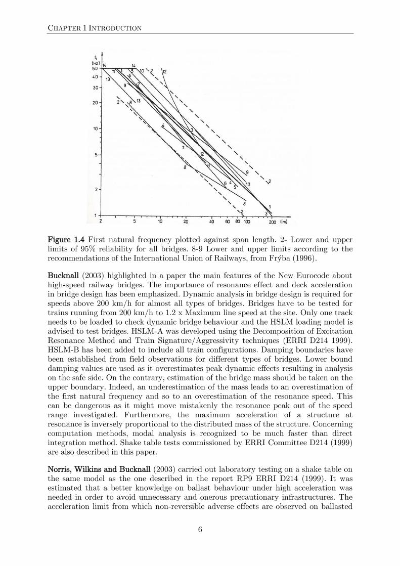
Frýba (1996) thoroughly investigated the dynamic of railway bridges, theoretically and experimentally. He wrote a state-of-the-art report of the existing theory about the behaviour of railway bridges under passing trains and pointed out the importance of first natural frequencies in bridge dynamic response. The influence of bridge parameters on bridge dynamic behaviour was outlined. Field experiments have been carried out on 113 railways distributed into five categories: steel truss bridge, steel plate girder with ballast, steel plate girder without ballast, concrete bridge with ballast and concrete bridge without ballast. Stiffness and first natural frequency were monitored and plotted against the span length. Boundaries for each category of bridge were drawn and expressed using regression functions. Natural frequency boundaries for each category of bridges are gathered in Figure 1.4. It points out that the first natural frequency of a bridge is always situated in a fixed interval for a given span length.
CHAPTER 1 INTRODUCTION
6
Figure 1.4 First natural frequency plotted against span length. 2- Lower and upper limits of 95% reliability for all bridges. 8-9 Lower and upper limits according to the recommendations of the International Union of Railways, from Frýba (1996).
Bucknall (2003) highlighted in a paper the main features of the New Eurocode about high-speed railway bridges. The importance of resonance effect and deck acceleration in bridge design has been emphasized. Dynamic analysis in bridge design is required for speeds above 200 km/h for almost all types of bridges. Bridges have to be tested for trains running from 200 km/h to 1.2 x Maximum line speed at the site. Only one track needs to be loaded to check dynamic bridge behaviour and the HSLM loading model is advised to test bridges. HSLM-A was developed using the Decomposition of Excitation Resonance Method and Train Signature/Aggressivity techniques (ERRI D214 1999). HSLM-B has been added to include all train configurations. Damping boundaries have been established from field observations for different types of bridges. Lower bound damping values are used as it overestimates peak dynamic effects resulting in analysis on the safe side. On the contrary, estimation of the bridge mass should be taken on the upper boundary. Indeed, an underestimation of the mass leads to an overestimation of the first natural frequency and so to an overestimation of the resonance speed. This can be dangerous as it might move mistakenly the resonance peak out of the speed range investigated. Furthermore, the maximum acceleration of a structure at resonance is inversely proportional to the distributed mass of the structure. Concerning computation methods, modal analysis is recognized to be much faster than direct integration method. Shake table tests commissioned by ERRI Committee D214 (1999) are also described in this paper.
Norris, Wilkins and Bucknall (2003) carried out laboratory testing on a shake table on the same model as the one described in the report RP9 ERRI D214 (1999). It was estimated that a better knowledge on ballast behaviour under high acceleration was needed in order to avoid unnecessary and onerous precautionary infrastructures. The acceleration limit from which non-reversible adverse effects are observed on ballasted

1.3 Literature review
7
tracks tallied with the one stipulated in the ERRI D214 (1999). After further studies, the authors suggest to increase the deck acceleration limit and to adapt it to the different types of existing bridges: 0.5 g for most susceptible ballasted bridges, 0.6 g for less susceptible ballasted tracks and 1,0 g for fully confined ballasted bridge. Experiments also highlighted that at the resonance frequency, the acceleration amplification factor is around three. Furthermore, the energy of the vibrations of frequencies higher than 50 Hz are negligible compared to lower frequencies. Consequently, the authors concluded that the maximum frequency that needs to be considered in an analysis is the maximum of 30 Hz or 1.5 times the third fundamental frequency but not more than 50 Hz.
Akiyama, Fukada and Kajikawa (2007) studied the influence of different structural systems on pedestrian and road single span bridge vibrations. They investigated four types of structural models: conventional, extended deck, semi-integral and integral bridges. Static, dynamic and ground vibrations have been studied. They found out that the integral bridge is the best solution regarding vibration problems. Their study pointed out the importance of structural models and ground vibration in bridge design.
Goicolea (2007) carried out a study following upon several collapses of bridges during their construction or utilisation. The signature, analytical method described in the report RP9 ERRI D214 (1999), was used to study the influence of bridge parameters on the first natural frequency, resonance speed and maximum vertical deck acceleration. Investigations were illustrated by examples on real bridges, relating design choices with maximum vertical acceleration.
Majka and Hartnett (2008) carried out an analysis to establish the key variables influencing the dynamic response of railway bridges. The speed of the train, train-to-bridge frequency, mass and span ratios, as well as bridge damping were identified as significant variables. Vehicle damping was found to have negligible influence on bridge response. Particularly strong dynamic amplification was found for train with shortly and regularly spaced axles travelling at the critical speeds. The dynamic behaviour of bridges under passing trains has been investigated by many other researchers during the last decade. Some important contributions are listed in Table 1.1.
Table 1.1 Other important contributions on bridge dynamic behaviour under moving load.
Authors Bridge Type Vehicle Model Description of the work
Xia et al. (2003) simply supported Thalys train experimental study
Björklund (2005) double-span HSLM-A train model finite element study
Xia et al. (2005) simply supported China-star train experimental study
Xia & Zhang (2005) simply supported China-star train theoretical and experimental study
Zhu & Law (2005) continuous Moving loads theoretical study
Liu et al. (2009) simply supported Moving loads and trains theoretical study
CHAPTER 1 INTRODUCTION
8
1.3.2 Optimization
Liang and Steven (2002) proposed an extension of a performance-based optimization method to produce optimal topologies of continuum structures. The performance-based optimization consists in designing “a structure or structural components that can perform physical functions in a specified manner throughout its design service life at minimum cost or weight.” The authors looked for minimizing the structure weight while satisfying the stiffness required. It has been noticed that under applied load, some regions of a structure are carrying more than others. From this observation, a loop was created to remove underutilized regions. Elements with the lowest strain energy densities were gradually eliminated. Taking into account the continuity and the symmetry of the structure, and studying the convergence of the performance index, an optimal design of the structure is found. Several examples of the method application are presented in the paper.
Jaishi and Ren (2006) updated a finite element model of the Hongtang Bridge, located at Fuzhou city in China. The influence of the objective function on the optimization algorithm behaviour and on the results is pointed out. Multi-objective optimisation was used in this analysis in order to overcome weighing difficulties in finite element updating. Besides, care should be taken in the physical significance of the result. All other finite element difficulties such as uncertainty, noise measurement, etc, are described in the paper. The function fmincon, gradient-based optimization method available in MATLAB, was used in this study.
Jonsson and Johnson (2007) worked on a finite element updated model of the New Svinesund Bridge. In order to improve the hand-updated model, different types of optimization function were considered. The Gradient-based method presents numerical difficulties in iterations and ill conditioning for the Jacobian and Hessian matrices. The Nelder-Mead Simplex algorithm appears to be the best option as it is more likely to escape local minima. Nevertheless, in a space containing many local minima, results of the optimization are highly dependent on the starting values. The optimization has to be run several times for different starting guesses to test for convergence.
Schlune, Plos and Gylltoft (2009) presented a state of the art of the finite element model updating of the Svinesund Bridge. The optimization process is accurately described, detailing the three main components: the updating parameters, the objective function, and the optimization algorithm. A risk of non-unique solutions problem in case of many updated parameters for few experimental data is pointed out. The different types of objective functions are listed. Besides, the optimization algorithms are described (Figure 1.5) and compared: the Nelder-Mead simplex algorithm is chosen as it is robust and does not requires the computation of any derivative contrary to gradient-based methods. Nevertheless, the Nelder-Mead algorithm is not able to find the global minimum in a problem with too many local minima. The genetic algorithm available in the MATLAB Global Optimization Toolbox has been used in order to find the global minimum.

1.3 Literature review
9
Figure 1.5 Classification of optimization methods, from Schlune et al. (2009).
Wiberg (2009) worked on a finite element updated model of the New Årsta Railway Bridge in Stockholm. The different parts of the optimization procedure and its implementation on MATLAB were described. The Nelder-Mead simplex algorithm was used, using the function fminsearch on MATLAB. In order to test and visualize the optimization process, a benchmark test with simple parameters was carried out. It highlighted the presence of local minima and showed the path the program takes to find the global minimum.


2.1 Parameters influencing bridge dynamic behaviour
11
Chapter 2 Method of analysis
The tools used to carry out the optimization study are presented in this chapter. First, the Train Signature used to calculate the maximum vertical deck acceleration of simply supported bridges is described. It is followed by the finite element modelling on ABAQUS used to compute the dynamic behaviour of double-span bridges. Finally, the optimization process is detailed.
2.1 Parameters influencing bridge dynamic behaviour
Bridge response under the action of a force depends on the characteristics of the bridge and the load applied. The key bridge parameters are the mass of the bridge, the length of the span, the first natural frequency of the bridge and the damping (ERRI D214 1999). Björklund (2005) carried out a study about the influence of the damping, the stiffness and the mass on the bridge dynamic behaviour. Tests have been done on a 45 m (2×22.5) double-span bridge under the influence of HSLM-A1 train. The results are presented in the following section (Figure 2.1 to Figure 2.6).
The first resonance speeds of a bridge due to axel repetition can be easily found with the equation:
v=f0×λ (2.1)
v is the critical speed in m/s; f0 is the first natural frequency of the bridge in Hz; λ is the regular axle distance in m.
The first natural frequency of the bridge studied by Björklund (2005) is around 4.3 Hz. The tests are carried out with the HSLM-A1 train, consequently the axle distance is 18 m (Figure 2.10): v=4.3×18=77.4 m/s=280 km/h
The first resonance speed of the bridge is around 280 km/h. The figures presented below confirm it.
CHAPTER 2 METHOD OF ANALYSIS
12
2.1.1 Bridge damping
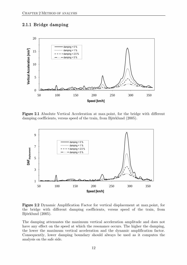
Figure 2.1 Absolute Vertical Acceleration at max.point, for the bridge with different damping coefficients, versus speed of the train, from Björklund (2005).
Figure 2.2 Dynamic Amplification Factor for vertical displacement at max.point, for the bridge with different damping coefficients, versus speed of the train, from Björklund (2005).
The damping attenuates the maximum vertical acceleration amplitude and does not have any effect on the speed at which the resonance occurs. The higher the damping, the lower the maximum vertical acceleration and the dynamic amplification factor. Consequently, lower damping boundary should always be used as it computes the analysis on the safe side.
0
5
10
15
20
50 100 150 200 250 300 350
Ver
tica
l Acc
eler
atio
n [
m/s
2 ]
Speed [km/h]
damping = 0 %
damping = 1 %
damping = 2.5 %
damping = 5 %
1
3
5
7
9
50 100 150 200 250 300 350
DA
Fd
isp
lace
men
t
Speed [km/h]
damping = 0 %
damping = 1 %
damping = 2.5 %
damping = 5 %

2.1 Parameters influencing bridge dynamic behaviour
13
2.1.2 Bridge stiffness
Figure 2.3 Absolute Vertical Acceleration at max.point, for the bridge with different stiffness, versus speed of the train, from Björklund (2005).
Figure 2.4 Dynamic Amplification Factor for vertical displacement at max.point, for the bridge with different stiffness, versus velocity of the train, from Björklund (2005).
Higher stiffness increases the first natural frequency and moves the resonance peak to higher speeds. Nevertheless, it does not have any effect on the amplitudes of the maximum vertical acceleration and the dynamic amplification factor. Thus, a lower bound value of the stiffness should be used in order to obtain a lower bound estimate of resonance speeds (Bucknall 2003).
0
2
4
6
8
10
50 100 150 200 250 300 350
Ver
tica
l Acc
eler
atio
n [m
/s2 ]
Speed [km/h]
E = 30 MPa
E = 35 MPa
E = 40 MPa
E = 45 MPa
1
2
3
4
5
6
50 100 150 200 250 300 350
DA
Fd
isp
lace
men
t
Speed [km/h]
E = 30 MPa
E = 35 MPa
E = 40 MPa
E = 45 MPa
CHAPTER 2 METHOD OF ANALYSIS
14
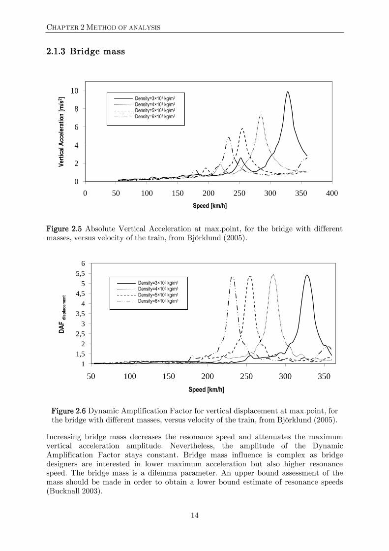
2.1.3 Bridge mass
Figure 2.5 Absolute Vertical Acceleration at max.point, for the bridge with different masses, versus velocity of the train, from Björklund (2005).
Figure 2.6 Dynamic Amplification Factor for vertical displacement at max.point, for the bridge with different masses, versus velocity of the train, from Björklund (2005).
Increasing bridge mass decreases the resonance speed and attenuates the maximum vertical acceleration amplitude. Nevertheless, the amplitude of the Dynamic Amplification Factor stays constant. Bridge mass influence is complex as bridge designers are interested in lower maximum acceleration but also higher resonance speed. The bridge mass is a dilemma parameter. An upper bound assessment of the mass should be made in order to obtain a lower bound estimate of resonance speeds (Bucknall 2003).
0
2
4
6
8
10
0 50 100 150 200 250 300 350 400
Ver
tica
l Acc
eler
atio
n [
m/s
2 ]
Speed [km/h]
1
1,5
2
2,5
3
3,5
4
4,5
5
5,5
6
50 100 150 200 250 300 350
DA
F d
isp
lace
men
t
Speed [km/h]
Density=3×10³ kg/m3
Density=4×10³ kg/m3
Density=5×10³ kg/m3
Density=6×10³ kg/m3
Density=3×10³ kg/m3
Density=4×10³ kg/m3
Density=5×10³ kg/m3
Density=6×10³ kg/m3
2.2 Train signature
15
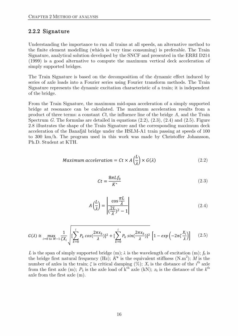
2.1.4 Summary
Bridge parameters influence on dynamic behaviour is summarised in Table 2.1.
Table 2.1 Influence of bridge characteristics on bridge dynamic behaviour.
Bridge parameters f0/resonance
speed max
acceleration
↗ Damping ξ no effect ↘
↗ Mass m ↘ with √m ↘
↗ Stiffness k ↗ with √k no effect
↗ Mass × Stiffness no effect ↘
2.2 Train signature
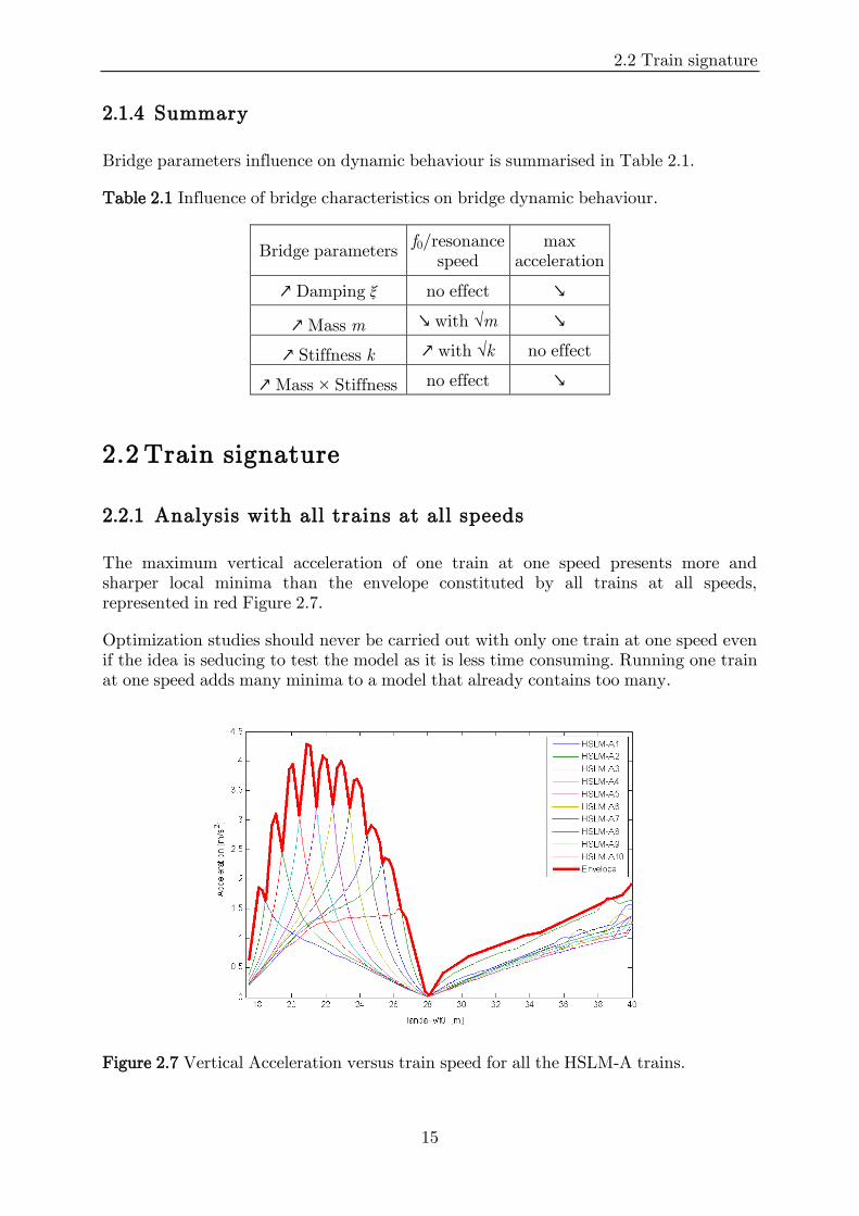
2.2.1 Analysis with all trains at all speeds
The maximum vertical acceleration of one train at one speed presents more and sharper local minima than the envelope constituted by all trains at all speeds, represented in red Figure 2.7.
Optimization studies should never be carried out with only one train at one speed even if the idea is seducing to test the model as it is less time consuming. Running one train at one speed adds many minima to a model that already contains too many.
Figure 2.7 Vertical Acceleration versus train speed for all the HSLM-A trains.
CHAPTER 2 METHOD OF ANALYSIS
16
2.2.2 Signature
Understanding the importance to run all trains at all speeds, an alternative method to the finite element modelling (which is very time consuming) is preferable. The Train Signature, analytical solution developed by the SNCF and presented in the ERRI D214 (1999) is a good alternative to compute the maximum vertical deck acceleration of simply supported bridges.
The Train Signature is based on the decomposition of the dynamic effect induced by series of axle loads into a Fourier series using Fourier transform methods. The Train Signature represents the dynamic excitation characteristic of a train; it is independent of the bridge.
From the Train Signature, the maximum mid-span acceleration of a simply supported bridge at resonance can be calculated. The maximum acceleration results from a product of three terms: a constant Ct, the influence line of the bridge A, and the Train Spectrum G. The formulas are detailed in equations (2.2), (2.3), (2.4) and (2.5). Figure 2.8 illustrates the shape of the Train Signature and the corresponding maximum deck acceleration of the Banafjäl bridge under the HSLM-A1 train passing at speeds of 100 to 300 km/h. The program used in this work was made by Christoffer Johansson, Ph.D. Student at KTH.
𝑀𝑎𝑥𝑖𝑚𝑢𝑚 𝑎𝑐𝑐𝑒𝑙𝑒𝑟𝑎𝑡𝑖𝑜𝑛 = 𝐶𝑡 × 𝐴 𝐿
𝜆 × 𝐺 𝜆 (2.2)
𝐶𝑡 =8𝜋𝐿𝑓0
𝐾∗ (2.3)
𝐴 𝐿
𝜆 =
cos𝜋𝐿𝜆
(2𝐿𝜆
)2 − 1 (2.4)
𝐺 𝜆 ≅ max𝑖=0 𝑡𝑜 𝑀−1
1
𝜁𝑋𝑖
[ 𝑃𝑘 𝑐𝑜𝑠(2𝜋𝑥𝑘
𝜆
𝑖
𝑘=0
)]2 + [ 𝑃𝑘 𝑠𝑖𝑛(2𝜋𝑥𝑘
𝜆
𝑖
𝑘=0
)]2 1 − 𝑒𝑥𝑝 −2𝜋𝜁𝑋𝑖
𝜆 (2.5)
L is the span of simply supported bridge (m); λ is the wavelength of excitation (m); f0 is the bridge first natural frequency (Hz); K* is the equivalent stiffness (N.m2); M is the number of axles in the train; ζ is critical damping (%); Xi is the distance of the ith axle from the first axle (m); Pk is the axle load of kth axle (kN); xk is the distance of the kth axle from the first axle (m).

2.3 ABAQUS modelling
17
Figure 2.8 HSLM-A1 Train Signature and deck acceleration of the Banafjäl bridge for speeds of 100 to 300 km/h.
2.3 ABAQUS modelling
2.3.1 Creation of the model
Bridge modelling
The bridges investigated are 2-D beams with simple boundary conditions; consequently, the ABAQUS modelling is rather simple. The bridge is constituted of beam elements and a generalized profile is used. The reader is invited to refer to Friswell and Mottershead, Chapter 2 (1995) if interested about the theory of finite element modelling.
Check of the bridge modelling: simple example of a 34 m span bridge
To check the program and the capacity of MATLAB to create a bridge on ABAQUS, a simple case is studied. The bridge example is taken from Karoumi (1998) where all the parameters and the natural frequency were available. The bridge is presented Figure 2.9.
10 15 20 25 30 350
2000
4000
6000
8000HSLM-A1 Train Signature
S0 (
kN
)
=v/f0 (m)
10 15 20 25 30 350
1
2
3
4Deck acceleration of the Banafjäl bridge
Deck a
ccele
ration (
m/s
2)
=v/f0 (m)

CHAPTER 2 METHOD OF ANALYSIS
18
Figure 2.9 Simply supported bridge subjected to a constant moving force, from Karoumi (1998).
The natural frequencies are calculated by two different manners. First with a model directly created on ABAQUS (using CAE interface), and then with a model created on MATLAB. The natural frequencies have been found exactly similar to the ones of Karoumi with the two methods. The program and the path between MATLAB and ABAQUS are therefore verified to work satisfactorily.
Modelling a train
Type of train
The HSLM-A trains presented in Figure 2.10 are used. The trains are represented as sets of concentrated loads. Point loads are considered sufficient to study dynamic behaviour of bridges as vehicle suspension system and damping have a negligible influence on the bridge response (Majka and Hartnett 2008).
A MATLAB code created by Raid Karoumi, Professor at KTH, is used to generate the 10 train models. For a given train type, it gives two vectors: one containing the amplitude of the point loads and one containing the position of the loads.
Speed of trains
The Eurocode advices to check bridges from 200 km/h to 1.2 x Maximum line speed at the site. As trains nowadays run up to 300 km/h, 350 km/h is chosen as upper speed limit. Thus, the bridges are checked for speeds from 150 km/h to 350 km/h.

2.3 ABAQUS modelling
19
Figure 2.10 High Speed Load Model HSLM-A description, from Eurocode (2002).
Creating a moving train
To model a train in ABAQUS, an amplitude function has to be defined. Each point load is considered to create a triangular amplitude. This one is defined between the node where the point load is applied and its two contiguous nodes, as shown in Figure 2.11. The full train is defined as a succession of moving triangular loads.
Figure 2.11 Triangular amplitude function for modelling a moving point load.
To make the train move, a corresponding time vector is built. The train moves forward by step equal to the size of the elements. Thus, an amplitude function depending on time is elaborated and written to an input file sent to ABAQUS.
Linear Dynamic analysis
Computation is carried out using the mode superposition technique. It is a time efficient method that is found to be accurate enough in previous studies, see for example Karoumi (1998).

CHAPTER 2 METHOD OF ANALYSIS
20
Frequencies considered
High-frequency vibrations are not believed to present any risk for ballast instability. Consequently, only lower modes need to be considered in dynamic analysis. Eurocode advices to check deck acceleration for frequencies up to the greater of 30 Hz or 1.5 times the frequency of the first mode of vibration of the element being considered. Frequencies up to 30 Hz have been considered in this study.
Check of bridge-train modelling: Brustjärnsbäcken bridge
In order to check the MATLAB program, the Brustjärnsbäcken bridge (Figure 2.12 and Table 2.2), presented in Karoumi & Wiberg (2006), has been investigated. A similar study as the one presented in their report has been carried out. The vertical deck acceleration is plotted as a function of the speed for each HSLM-A train. Calculations are made by mode analysis, including only 3 modes and the speeds are going from 50 to 300 km/h. The bridge is made of 70 beam elements and the time step is 0.0019 s.
Figure 2.12 The Brustjärnsbäcken bridge on the Bothnia Line, from Karoumi and Wiberg (2006).
Table 2.2 Brustjärnsbäcken parameters.
Input data
L 35 m
A 6.39 m2
I 2.62 m4
ρ 3924 kg/m3
E 32 GPa
material prestressed concrete
In Figure 2.13, Karoumi and Wiberg results are plotted next to the present results. The curves are very close. The few differences are probably due to differences in the software such as element definitions. Thus, the train and bridge modelling is found to work accurately and satisfactorily.

2.3 ABAQUS modelling
21
Figure 2.13 Vertical acceleration as a function of the train speed, for the HSLM-A trains, including only 3 modes. Karoumi & Wiberg curves are in full lines, Mellier curves in dashed lines.
2.3.2 Convergence study
A convergence study on mesh size and sampling frequency has to be carried out for each span length. As an example, the analysis for the 42 m long Banafjäl bridge, situated on the Bothnia line, is presented below. The convergence studies have been made with the train and at the speed that give the maximum vertical acceleration on the Banafjäl bridge (train HSLM-A3 at 170 km/h gives the vertical acceleration 6.26 m/s2).
The Banafjäl Bridge
The Banafjäl bridge is a 42 m long composite simply supported bridge situated on the Bothnia line. Its dynamic behaviour has been thoroughly studied in Karoumi and Wiberg (2006). Its characteristics are presented in Table 2.3.
Table 2.3 Banafjäl bridge parameters.
Input data
L 42 m
A 0.57 m2
I 0.62 m4
ρ 31825 kg/m3
E 210 GPa
material composite
50 100 150 200 250 3000
2
4
6
8
10
12
Vert
ical a
ccele
ratio
n (
m/s
2)
Train speed (km/h)
HSLM-A1 Karoumi & Wiberg
HSLM-A2 Karoumi & Wiberg
HSLM-A3 Karoumi & Wiberg
HSLM-A4 Karoumi & Wiberg
HSLM-A5 Karoumi & Wiberg
HSLM-A6 Karoumi & Wiberg
HSLM-A7 Karoumi & Wiberg
HSLM-A8 Karoumi & Wiberg
HSLM-A9 Karoumi & Wiberg
HSLM-A10 Karoumi & Wiberg
HSLM-A1 Mellier
HSLM-A2 Mellier
HSLM-A3 Mellier
HSLM-A4 Mellier
HSLM-A5 Mellier
HSLM-A6 Mellier
HSLM-A7 Mellier
HSLM-A8 Mellier
HSLM-A9 Mellier
HSLM-A10 Mellier

CHAPTER 2 METHOD OF ANALYSIS
22
Mesh size
In order to know how fine the mesh has to be, the natural frequencies are plotted as a function of the number of elements for the different frequencies taken into account in the study (that is to say up to 30 Hz). The results are presented in Figure 2.14.
Figure 2.14 Natural frequencies as a function of the number of elements.
It appears that the natural frequencies are stable from around 15 elements. Nevertheless, the mesh size is also closely related to the time step convergence. Therefore, further studies are required.
Time Step
The time step has a great influence on the time of the analysis. Multiplying the time step by 2 divides approximately the analysis time by 2. Therefore, the time step has to be chosen from a compromise between accuracy of the results and analysis time.
The maximum vertical acceleration is plotted as a function of the time step for different numbers of elements (Figure 2.15). The time step and the mesh size do not influence much the calculations of the maximum vertical acceleration. From this plot, 6 ms seems to be a suitable time step.
5 10 15 20 25 30 35 40 45 502
4
6
8
10
12
14
16
18
20
22
Number of elements
Na
tura
l fr
eq
ue
ncy (
Hz)
f2
f1
f4
f3

2.3 ABAQUS modelling
23
Figure 2.15 Time Step Convergence Analysis for B21 elements. Absolute maximum vertical acceleration against time step.
A time step convergence analysis has also been carried out for B23 elements (see also next section). The result is more sensitive to time step than with B21 elements. Consequently, a smaller time step would be needed for a study with Euler-Bernouilli elements (B23), involving longer analysis.
Figure 2.16 Time Step Convergence Analysis for B23 elements. Maximum vertical acceleration against time step.
Element type
To model 2-D beams, ABAQUS offers two types of elements: the Euler-Bernoulli beams, called B23 element, and the Timoshenko beams, called B21 element. The main difference between these elements is that the Euler-Bernoulli element does not take into account shear deformation, whereas the Timoshenko element does. Therefore, the latter is used for high beams and the first for normal beams where shear deformations
1 2 3 4 5 6 7 8 9 10
x 10-3
6.275
6.28
6.285
6.29
6.295
6.3
6.305
6.31
Time step (s)
Maxim
um
vert
ical accele
ration (
m/s
2)
71 Nodes
151 Nodes
301 Nodes
1 2 3 4 5 6 7 8 9 10
x 10-3
6.04
6.05
6.06
6.07
6.08
6.09
6.1
6.11
6.12
6.13
6.14
Time step (s)
Maxim
um
vert
ical accele
ration (
m/s
2)
71 Nodes
151 Nodes

CHAPTER 2 METHOD OF ANALYSIS
24
are less important. However, the Timoshenko element usually requires more analysis time and as testing the ten trains for all the speeds is time-consuming, reducing analysis time is an important issue. Thus, a quick study has been made on analysis times. The time has been regarded as a function of the time step frequency for the two types of elements (Figure 2.17).
Figure 2.17 Time of the analysis as a function of time step.
For a time step larger than 0.003 s, the analysis time does not depend on the type of element. The Timoshenko element seems to be more interesting as it includes shear effects. This type of element is also used by Schlune et al. (2009).
Analysis parameters
The mesh size study showed that the frequencies are not influenced by the number of elements if the latter is superior to 15.
The time step study showed that 70 elements and a time step of 6 ms give a satisfactory accuracy, which is better with Timoshenko elements than with Euler-Bernoulli elements.
The element type study showed that both types of elements take the same analysis time.
Timoshenko elements are more appropriate for the study as they save time and include shear deformation (and so they are valid for all types of beams.) Consequently, the bridge is modelled by 70 Timoshenko beam elements and sampled with a time step of 6 ms.
2 2.5 3 3.5 4 4.5 5 5.5 6
x 10-3
20
30
40
50
60
70
80
90
100
110
Time step (s)
Analy
sis
tim
e (
s)
B21
B23
2.3 ABAQUS modelling
25
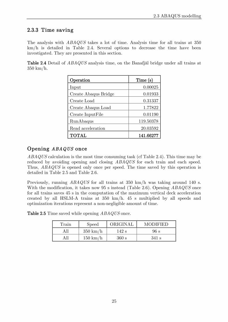
2.3.3 Time saving
The analysis with ABAQUS takes a lot of time. Analysis time for all trains at 350 km/h is detailed in Table 2.4. Several options to decrease the time have been investigated. They are presented in this section.
Table 2.4 Detail of ABAQUS analysis time, on the Banafjäl bridge under all trains at 350 km/h.
Operation Time (s)
Input 0.00025
Create Abaqus Bridge 0.01933
Create Load 0.31337
Create Abaqus Load 1.77822
Create InputFile 0.01190
RunAbaqus 119.50378
Read acceleration 20.03592
TOTAL 141.66277
Opening ABAQUS once
ABAQUS calculation is the most time consuming task (cf Table 2.4). This time may be reduced by avoiding opening and closing ABAQUS for each train and each speed. Thus, ABAQUS is opened only once per speed. The time saved by this operation is detailed in Table 2.5 and Table 2.6.
Previously, running ABAQUS for all trains at 350 km/h was taking around 140 s. With the modification, it takes now 95 s instead (Table 2.6). Opening ABAQUS once for all trains saves 45 s in the computation of the maximum vertical deck acceleration created by all HSLM-A trains at 350 km/h. 45 s multiplied by all speeds and optimization iterations represent a non-negligible amount of time.
Table 2.5 Time saved while opening ABAQUS once.
Train Speed ORIGINAL MODIFIED
All 350 km/h 142 s 96 s
All 150 km/h 360 s 341 s
CHAPTER 2 METHOD OF ANALYSIS
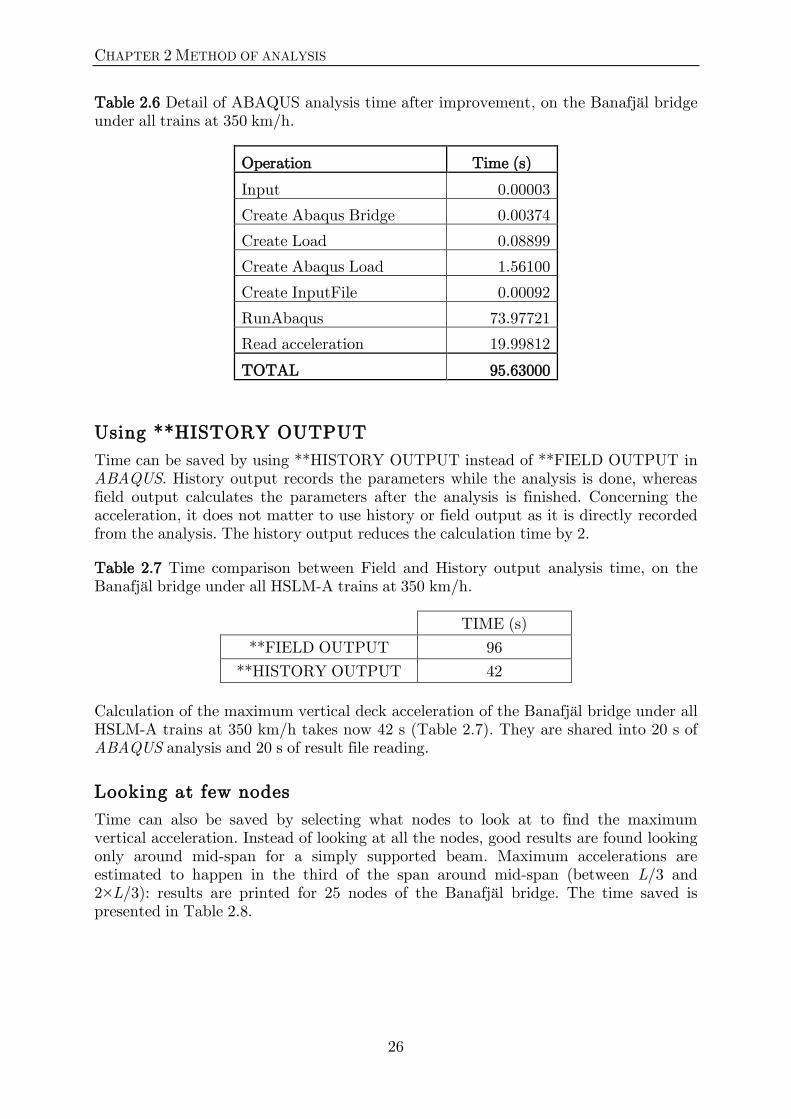
26
Table 2.6 Detail of ABAQUS analysis time after improvement, on the Banafjäl bridge under all trains at 350 km/h.
Operation Time (s)
Input 0.00003
Create Abaqus Bridge 0.00374
Create Load 0.08899
Create Abaqus Load 1.56100
Create InputFile 0.00092
RunAbaqus 73.97721
Read acceleration 19.99812
TOTAL 95.63000
Using **HISTORY OUTPUT
Time can be saved by using **HISTORY OUTPUT instead of **FIELD OUTPUT in ABAQUS. History output records the parameters while the analysis is done, whereas field output calculates the parameters after the analysis is finished. Concerning the acceleration, it does not matter to use history or field output as it is directly recorded from the analysis. The history output reduces the calculation time by 2.
Table 2.7 Time comparison between Field and History output analysis time, on the Banafjäl bridge under all HSLM-A trains at 350 km/h.
TIME (s)
**FIELD OUTPUT 96
**HISTORY OUTPUT 42
Calculation of the maximum vertical deck acceleration of the Banafjäl bridge under all HSLM-A trains at 350 km/h takes now 42 s (Table 2.7). They are shared into 20 s of ABAQUS analysis and 20 s of result file reading.
Looking at few nodes
Time can also be saved by selecting what nodes to look at to find the maximum vertical acceleration. Instead of looking at all the nodes, good results are found looking only around mid-span for a simply supported beam. Maximum accelerations are estimated to happen in the third of the span around mid-span (between L/3 and 2×L/3): results are printed for 25 nodes of the Banafjäl bridge. The time saved is presented in Table 2.8.

2.3 ABAQUS modelling
27
Table 2.8 Comparison of analysis time for checking the acceleration at all nodes and at only 25 nodes.
Nodes TIME (s) amax
All (71) 42 1.996
25 25 1.996
Analysis with all nodes takes 42 s shared into 20 s of ABAQUS analysis and 20 s of result file reading, whereas analysis with 25 nodes takes 25 s shared into 14 s of ABAQUS analysis and 9 s of result file reading. By selecting nodes, time is most of all saved on file reading.
To check the conformity of the values calculated with 25 nodes to those calculated with all nodes, the absolute maximum acceleration per speed for all 10 trains have been computed. Results are plotted in Figure 2.18. Slight differences occur between the two analyses at low acceleration. At resonance speeds, the maximum vertical acceleration at 25 nodes complies with the study at all nodes. As the study focuses on the maximum vertical acceleration of all speeds, the interesting results are those around resonance. Consequently, checking acceleration at the 25 nodes around bridge mid-point are enough to give satisfying and accurate results for this bridge.
Figure 2.18 Absolute maximum vertical acceleration of all HSLM-A trains against speed.
Total Analysis Time
Analysis for all trains at all speeds takes now around 22 min, against 134 min before any attempt to optimize the time (Table 2.9).
Table 2.9 Summary of analysis time reduction.
Original 134 min
Opening ABAQUS once + History output 40 min
Opening ABAQUS once + History output + Only 25 Nodes 22 min
150 200 250 300 3501
2
3
4
5
6
7
Speed (km/h)
Absolu
te m
axim
um
vert
ical accele
ration (
m/s
2)
all nodes
25 nodes

CHAPTER 2 METHOD OF ANALYSIS
28
Further ideas not investigated
These two ideas are believed to save a large amount of time. They have not been investigated because they are time consuming to implement and this master thesis focuses on optimization of bridges parameters and not of ABAQUS analysis time.
Testing only speeds around resonance speed
As the study aims at determining the absolute maximum vertical deck acceleration there is no need to compute every value for each train each speed. Speeds around resonance are enough to find the maximum acceleration for each type of train. The resonance speed can be easily estimated with v=f0×λ (presented at the beginning of this chapter). Thus, instead of calculating the maximum acceleration for all trains at all speeds, only speeds around resonance are checked for each train.
Creating a result file .fil instead of .dat
A very efficient way to save time in an ABAQUS study is to use a .fil instead of a .dat as a results file. A .fil is a binary file and data have to be extracted with a subroutine, which makes its use more complicated than a .dat file. An example of data extraction from .fil can be found in Appendix C.5 of Flemming, Hasselberg and Gillesén (2000).
2.4 Optimization
2.4.1 General description of the optimization loop
The loop to optimize cross sections of double-span bridges is presented Figure 2.19 and those of simply supported bridges in Figure 2.20. In Figure 2.19, optimization, creation of input file and reading of result file are carried out in MATLAB; calculation of the vertical acceleration are implemented in the finite element software ABAQUS. The MATLAB files corresponding to this loop are presented in Appendix A. In Figure 2.20, the train signature is used to calculate acceleration of simply supported bridges, all the analysis is carried out in MATLAB.
Figure 2.19 Optimization loop for double-span bridges, inspired from Flemming et al. (2000).
Initial design: Cross section parameters are introduced as a starting point of the optimization process. The initial design is taken close to an existing bridge.
Input file: From the initial parameters, MATLAB makes an input file to create the corresponding bridge FE model and the load vectors.

2.4 Optimization
29
FE Analysis: ABAQUS creates the model, runs the analysis and produces a result file.
Maximum acceleration: MATLAB reads the result file and extract the maximum and minimum vertical acceleration at each sampling time. Then, MATLAB sends the absolute maximum vertical acceleration to the optimization routine.
New design: The optimization routine on MATLAB evaluates the result, compares it to 3,5 m/s2, checks the constraints if any, and chooses new design parameters that are sent to MATLAB for a new input file to be created, etc.
The loop with the Train Signature is based on the same model. The only difference is the direct computation in MATLAB of the maximum vertical deck acceleration.
Figure 2.20 Optimization loop for simply supported bridges, inspired from Flemming et al. (2000).
2.4.2 Optimization process
Non-linear optimization contains three main components: the updating parameters, the objective function, and the optimization algorithm.
The updating parameters are the bridge parameters that are optimized. Several parameters influence dynamic behaviour of the structure under passing train. Those are listed in the Eurocode:
- Vehicle parameters: speed, axle spacing, axle load, suspension characteristics, vehicle imperfections...
- Bridge parameters: span length L, the mass of the structure m, the damping of the structure, the modulus of elasticity E and the second moment of inertia I.
- Track parameters: vertical irregularities, dynamic characteristics, presence of regularly spaced supports...
The aim of this work is to find the optimized bridge parameters. Consequently, track parameters are neglected and vehicles parameters do not need to be investigated as the HSLM-A trains are used to test the structures.
Each study is done for given span length and material, and the damping is taken according to the Eurocode. In this report, the updating parameters are either the area, the stiffness and the mass of the cross section, or the dimensions. The updating parameters vector has to be unit-less so that the choice of units and different scales of parameters do not influence the optimization (Schlune et al. 2009).

CHAPTER 2 METHOD OF ANALYSIS
30
The objective function represents the evaluation of the error between the finite element analysis result and the target, that is to say between the maximum vertical acceleration calculated by ABAQUS or the Train Signature and the Eurocode limit (3.5 m/s2). There exist numerous objective functions that are widely described in Schlune et al (2009). Since there is only one parameter in this study, the maximum vertical deck acceleration, the different objective functions can be reduced to one unique:
𝑂𝑏𝑗𝑒𝑐𝑡𝑖𝑣𝑒 𝑓𝑢𝑛𝑐𝑡𝑖𝑜𝑛 = 3.5 − 𝑎 𝑝
3.5 (2.6)
The optimization algorithm is the method used to optimize the updating parameters from the objective function values. It influences the speed, the efficiency and the results of the analysis. Its choice is crucial in the optimization process. Schlune et al. (2009) pointed out that the Gauss-Newton is probably the most often used algorithm for FE model updating but that Rosenbrock’s methods and global optimization algorithms have also been applied for that purpose. The Nelder-Mead simplex algorithm is also popular for FE model updating; it has been used by Jonsson and Johnson (2007), Schlune et al. (2009) and Wiberg (2009).
2.4.3 Optimization in MATLAB
MATLAB contains eleven minimization functions in the Optimization Toolbox. The choice of the function is made regarding the presence or not of constraints, the type of the objective function and the linearity of the problem.
Fminsearch is an unconstrained non-linear optimization tool using the Nelder-Mead simplex algorithm. It is a robust algorithm that is likely to escape local minima. It has been used in finite element model updating by Jonsson and Johnson (2007), Schlune et al. (2009), and Wiberg (2009).
Fmincon is a constrained non-linear optimization tool using the Sequential Quadratic Programming (SQP), a gradient-based method. It gives the possibility to put constraints to the updating parameters but requires the computation of derivatives, which is time consuming. It presents numerical difficulties in iterations and ill conditioning for the Jacobian and Hessian matrices (Jonsson and Johnson, 2007). It has been used by Jaishi and Ren (2006) for finite element model updating.
Optimize, available on MATLAB Central (created by Mr Rody Oldenhuis. http://www.mathworks.com/matlabcentral/fileexchange/24298-optimize), is a function that optimizes general constrained problems using Nelder-Mead algorithm. It is a non-gradient based method and consequently is faster than fmincon (which requires the computation of derivatives and so several evaluations per iteration). It is more stable and constraints can be put on updating parameters.

2.4 Optimization
31
However, whatever the choice of the algorithm, in a space containing many local minima, results of the optimization are highly dependent on the starting values. The optimization has to be run several times for different starting guesses to test for convergence.
Genetic algorithm, available in the MATLAB Global Optimization Toolbox, is based on the principles of biological evolution. It is “repeatedly modifying a population of individual points using rules modelled on gene combinations in biological reproduction.” (Mathworks website. Description of the Genetic algorithm). Due to its random nature, the chances to find the global minimum are increased. Nevertheless, this algorithm is time consuming and included in an expensive toolbox of MATLAB. It has been used by Schlune et al. (Schlune 2010).
Godlike available on MATLAB Central, combines four global optimizers. It increases robustness but not efficiency. As it runs four algorithms at a time, it is very time-consuming. When tried, for only one train, one speed, the optimization took more than 24 hours (and has been stopped before it ended). This algorithm requires powerful computers.
2.4.4 Realistic constraints
From extensive field tests, Frýba concluded that “The most important dynamic characteristics of railway bridges are their natural frequencies which actually characterize the extent to which the bridge is sensitive to dynamic loads” (1996:66). Figure 2.21 presents the first natural frequency of bridges as a function of the span length. This graph is part of the tools presented in the Eurocode to help to determine if a dynamic analysis of a bridge is needed or not.
It can be noticed that these boundaries coincides with Frýba’s graph (Figure 1.4) that shows the repartition of first natural frequency against span length for existing bridges. Consequently, in this master thesis, the grey zone was considered as a proof of the feasibility of the bridge. Indeed, optimization can give parameters combinations with no physical meaning. In order to create only realistic bridges, constraints needed to be added. Bridges were considered realistic if their first natural frequency was fitting in the boundaries presented Figure 2.21.

CHAPTER 2 METHOD OF ANALYSIS
32
Figure 2.21 First natural frequency boundaries, from Eurocode (2002).
2.4.5 Importance of starting values and comparison of fmincon and optimize
Fmincon and optimize are both optimization functions that let the user introduce constraints on parameters. As said earlier, fmincon uses Sequential Quadratic Programming (SQP) method while optimize uses Nelder-Mead simplex algorithm. Their efficiency is studied below on a 25 m prestressed concrete simply supported bridge. The second moment of inertia I and the cross section mass M are optimized in order to fit the maximum vertical acceleration criterion 3.5 m/s2. I can vary between 1 m4 and 4 m4 and M between 2721 kg/m and 72561 kg/m. The updating parameters are normalised in the vector p. p=[I/I0 M/M0] with I0=0.62 m4; M0=18140.25 kg/m. Besides, parameters are constrained for the first natural frequency to stay in the boundaries defined in the Eurocode (Figure 2.21) for a 25 m long bridge. The characteristics of the bridge are presented in Table 2.10.
Table 2.10 Input data of the 25 m concrete simply supported bridge.
Input data
L 25 m
E 35 GPa
I 1 < I < 4 m4
M 2721 < M < 72561 kg/m
f0 3.51 < f0 < 8.53 Hz
material prestressed concrete

2.4 Optimization
33
Previously to the optimization analysis, the maximum vertical acceleration has been computed for each combination of I and M contained in the boundaries (on the updating parameters and first natural frequency). For that purpose, the program created by Johan Wiberg, Ph.D. at KTH, to carry out his benchmark test has been used. The program is available in Appendix B. p(I)1 varies between 1.6 and 6.45 and p(M) between 0.15 and 4. Both are incremented by steps of 0.05. Bridge parameters with first natural frequency out of boundaries have been deleted. Figure 2.22, the objective function values are plotted as a function of the updating parameters. The thin lines represent the levels of objective function values. The bluer part represents the values of the objective function the closer to 0. The acceleration corresponding to the levels shown in Figure 2.22 are presented in Table 2.12. The suitable minima (objective function value below 0.06) are hatched.
Several optimization tests have been carried out for different starting values. The results are shown in Table 2.11 and paths taken by the algorithms are shown in Figure 2.22.
First, the optimization is launched from a starting vector p0=[5.5 1.5]. As the starting values are close to the suitable minima, both algorithms end to a correct solution. Nevertheless, starting with the vector p0=[5 1], the Nelder-Mead simplex algorithm finds a satisfying solution while the SQP method does not, the latter stops at the boundary of the study. This reflects the better capacity of the non-gradient based method to overcome local minima, as pointed out by Jonsson and Johnson (2007). It is confirmed by the fact that, for the starting value p0=[4 1.5], the Nelder-Mead simplex algorithm (thick red line in Figure 2.22) crosses several up-and-downs while the SQP method (thick green line in Figure 2.22) gets stuck just next to the starting point. The zooms show that both algorithms end at the bottom of a wall.
When the starting values are too far from the global minima, both algorithms are stuck in local minima. It has to be kept in mind that the algorithm stops when the convergence criterion is satisfied even if the value of the acceleration is far from the target value. This shows the importance of the starting values, which determine in what basin the algorithm is going to stay stuck.
Table 2.11 Results of the optimization with fmincon and optimize.
Optimize Fmincon
p0 pfinal acc Objval f0 pfinal acc Objval f0
[5.5 1.5] [5.5651 1.5053] 3.5000 3.48E-06 5.29 [5.4965 1.5056] 3.4999 2.31E-05 5.25
[5 1] [5.3998 1.4964] 3.4999 2.47E-05 5.22 [6.4500 1.2875] 4.0543 1.58E-01 6.15
[6 1] [6.3649 1.4997] 3.4999 2.16E-05 5.66 [6.1695 0.6423] 3.5006 1.65E-04 8.52
[4 1.5] [6.3431 2.6244] 6.5668 8.76E-01 4.27 [3.9997 1.6548] 9.3549 1.67E+00 4.27
[2 3] [6.4500 3.3659] 6.3254 8.07E-01 3.81 [6.4499 3.3659] 6.6791 9.08E-01 3.81
1 p(I)=p(1)=I/I0 and p(M)=p(2)=M/M0.

CHAPTER 2 METHOD OF ANALYSIS
34
Table 2.12 Equivalence between levels and acceleration ranges.
Level Acceleration range
0.015 between 3.45 and 3.55 m/s2
0.060 between 3.3 and 3.7 m/s2
0.200 between 2.8 and 4.2 m/s2
0.400 between 2.1 and 4.9 m/s2
Figure 2.22 Objective function value plotted as a function of I/I0 and M/M0. The bluer part represents the values of the objective function the closer to 0. Optimization algorithms paths in thick lines: optimize in red and fmincon in green.
0.0150.015
0.06
0.06
0.2
0.2 0.2
0.4
0.4
0.4 0.4
0.4
0.6
0.6
0.6
0.6 0.6
0.6
0.6 0.6
1
1
1
1
1
1
1
1
1
111
1.5
1.5
1.5
1.5
1.5
1.5
1.5
2
2
2
2
2
Normalised second moment of inertia I/I0
No
rma
lise
d c
ross s
ectio
n m
ass M
/M0
3.5 4 4.5 5 5.5 6
0.5
1
1.5
2
2.5
3
Suitable minima
Optimize final value
Optimize final value
Fmincon final value
Starting value [5 1]
Fmincon final value
Starting value [4 1.5]
0.688960.68896
0.71664
0.71664
0.71664
0.71664
0.74432
0.74432
0.74432
0.74432
0.74432
0.74432
0.74432
0.7720.772
0.772
0.772
0.772
0.772
0.772
0.772
0.79967
0.79967
0.79967
0.79967
0.79967
0.79967
0.82735
0.82735
0.82735
0.82735
0.85503
0.85503
0.85503
0.85
503
0.88271
0.88271
0.88271
0.88271
0.88271
0.88271
0.91039
0.9
10
39
0.91039
0.91039
0.9
38
07
0.93807
Normalised second moment of inertia I/I0
Norm
alis
ed c
ross s
ection m
ass M
/M0
6.1 6.15 6.2 6.25 6.3 6.35 6.4 6.452.45
2.5
2.55
2.6
2.65
2.7
2.75
1.6692 1.6692
1.66921.6692
1.7098
1.7098
1.7098 1.70981.7098
1.7098
1.70981.7098
1.7503
1.7503
1.7503
1.7503
1.75031.7503
1.7503
1.7503
1.7503
1.75031.7503 1.7503
1.7909
1.7909
1.7909
1.7909
1.79091.7909
1.7909
1.7909
1.7909
1.7909
1.7909 1.7909 1.7909
1.83141.8314
1.8314
1.8314
1.8314
1.8314
1.83141.8314
1.8314
1.8314
1.8719
1.8719
1.8719
1.8719
1.8719
1.9125
1.9125
1.9125
1.9531.953
1.953
1.953
1.953
1.953
1.99361.9936
1.9936
1.9936
2.0341
2.0341
Normalised second moment of inertia I/I0
Norm
alis
ed c
ross s
ection m
ass M
/M0
3.9 3.92 3.94 3.96 3.98 4 4.02 4.04 4.06 4.08
1.45
1.5
1.55
1.6
1.65
1.7
1.75
2.4 Optimization
35
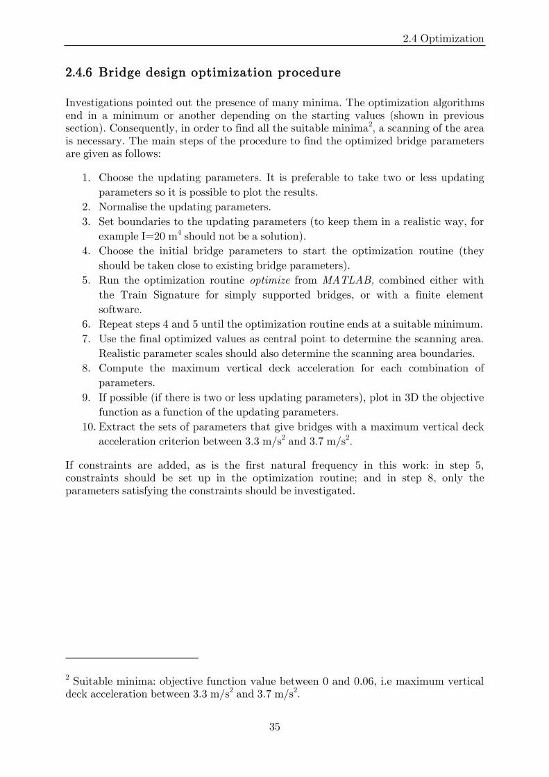
2.4.6 Bridge design optimization procedure
Investigations pointed out the presence of many minima. The optimization algorithms end in a minimum or another depending on the starting values (shown in previous section). Consequently, in order to find all the suitable minima2, a scanning of the area is necessary. The main steps of the procedure to find the optimized bridge parameters are given as follows:
1. Choose the updating parameters. It is preferable to take two or less updating
parameters so it is possible to plot the results.
2. Normalise the updating parameters.
3. Set boundaries to the updating parameters (to keep them in a realistic way, for
example I=20 m4 should not be a solution).
4. Choose the initial bridge parameters to start the optimization routine (they
should be taken close to existing bridge parameters).
5. Run the optimization routine optimize from MATLAB, combined either with
the Train Signature for simply supported bridges, or with a finite element
software.
6. Repeat steps 4 and 5 until the optimization routine ends at a suitable minimum.
7. Use the final optimized values as central point to determine the scanning area.
Realistic parameter scales should also determine the scanning area boundaries.
8. Compute the maximum vertical deck acceleration for each combination of
parameters.
9. If possible (if there is two or less updating parameters), plot in 3D the objective
function as a function of the updating parameters.
10. Extract the sets of parameters that give bridges with a maximum vertical deck
acceleration criterion between 3.3 m/s2 and 3.7 m/s2.
If constraints are added, as is the first natural frequency in this work: in step 5, constraints should be set up in the optimization routine; and in step 8, only the parameters satisfying the constraints should be investigated.
2 Suitable minima: objective function value between 0 and 0.06, i.e maximum vertical deck acceleration between 3.3 m/s2 and 3.7 m/s2.


3.1 Simply supported composite bridge
37
Chapter 3 Analysis and results
The investigations and results from optimizing the cross section of typical bridge types are presented in this chapter. The structures studied are single-track simply supported bridges: composite, ordinary and prestressed concrete; and double-span ordinary concrete bridges. The dynamic behaviour of simply supported bridges has been computed with the Train Signature whereas the behaviour of double-span bridges has been modelled in ABAQUS.
3.1 Simply supported composite bridge
The optimization of a composite bridge section is the subject of the first investigations. The Banafjäl bridge (simply supported 42 m span composite bridge) is the starting point of these tests. Its characteristics are taken as reference values. The updating parameters are normalised with its parameters (Table 3.1). The ballast weight is included in the mass of the bridge.
Table 3.1 Banafjäl bridge parameters.
Input data
L 42 m
A 0.57 m2
I 0.62 m4
ρ 31825 kg/m3
M 18140.25 kg/m
E 210 GPa
material composite

CHAPTER 3 ANALYSIS AND RESULTS
38
3.1.1 Optimization tests with fminsearch, fmincon and optimize
Several algorithms, updating parameters and starting values have been tried to optimize the Banafjäl bridge cross section regarding the maximum vertical deck acceleration criterion. The tests are presented below.
The MATLAB function fminsearch has first been tried as it is commonly used in updating model optimization. Nevertheless, as this function does not allow the set up of any boundaries, the solutions present too low first natural frequencies compared to Eurocode’s values. They are therefore considered as unrealistic. Table 3.2 shows the results.
Table 3.2 Results of the optimization with fminsearch.
p0 pfinal Objval f0
[A/A0 I/I0 ρ/ρ0] [1 1 1] [1.1770 0.6757 1.1576] 2.24E-05 1.68
[0.6 0.6 0.6] [1.1936 0.2886 1.4209] 5.85E-05 0.98
The only non-linear constrained optimization function available in the MATLAB Optimization Toolbox is fmincon. Constraints are put on the first natural frequency, which should lie between 2.58 Hz and 5.79 Hz for a 42 m span bridge (Figure 2.21). Results with fmincon are presented in Table 3.3. The function finds many solutions highly dependent on the starting values. These solutions are realistic regarding the first natural frequency of the structure but not regarding the values of the parameters. The stiffness is too big. In a second time, the number of updating parameters has been decreased but the problem keeps presenting many minima.
Table 3.3 Results of the optimization with fmincon.
Parameters boundaries
p0 pfinal Objval f0
[A/A0 I/I0 ρ/ρ0] 0.01<p<8 [1 1 1] [1.4103 6.6340 1.4089] 1.74E-05 4.36
[0.6 0.6 0.6] [1.3249 4.2649 1.5001] 2.94E-05 3.50
[0.8 0.8 0.8] [1.4031 2.3442 1.4048] 7.37E-05 2.60
[0.9 0.9 0.9] [1.4014 3.0364 1.4014] 5.47E-05 2.97
0.01<p<2 [0.9 0.9 0.9] [1.3078 2.000 1.3078] 0.1622 2.58
[0.6 0.6 0.6] [1.3078 2.000 1.3078] 0.1622 2.58
0.01<p<2.5 [0.6 0.6 0.6] [1.3812 2.500 1.3778] 0.0299 2.73
[I/I0 M/M0] 0.01<p<8 [0.6 0.6] [3.3049 1.9880] 1.29E-05 3.08
[1 1] [7.1298 1.8623] 1.11E-06 4.67
[0.4 0.4] [4.0851 0.7529] 2.84E-05 5.56
[0.1 0.1] [4.1889 1.9770] 3.57E-04 3.47
I/I0 0.01<p<8 1 4.8594 0.0791 5.26
0.5 3.1513 0.9596 4.24
0.1 5.6059 0.2342 5.65
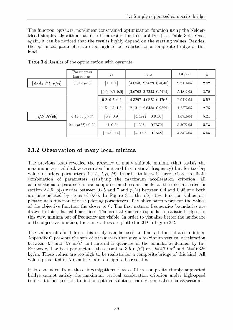
3.1 Simply supported composite bridge
39
The function optimize, non-linear constrained optimization function using the Nelder-Mead simplex algorithm, has also been tested for this problem (see Table 3.4). Once again, it can be noticed that the results highly depend on the starting values. Besides, the optimized parameters are too high to be realistic for a composite bridge of this kind.
Table 3.4 Results of the optimization with optimize.
Parameters boundaries
p0 pfinal Objval f0
[A/A0 I/I0 ρ/ρ0] 0.01<p<8 [1 1 1] [4.0848 2.7529 0.4840] 9.21E-05 2.82
[0.6 0.6 0.6] [3.6702 2.7233 0.5415] 5.48E-05 2.79
[0.2 0.2 0.2] [4.3297 4.0828 0.1762] 2.01E-04 5.52
[1.5 1.5 1.5] [2.1311 2.6488 0.9329] 1.23E-05 2.75
[I/I0 M/M0] 0.45<p(I)<7 [0.9 0.9] [4.4927 0.9431] 1.07E-04 5.21
0.4<p(M)<0.95 [4 0.7] [4.2534 0.7370] 5.50E-05 5.73
[0.45 0.4] [4.0905 0.7548] 4.84E-05 5.55
3.1.2 Observation of many local minima
The previous tests revealed the presence of many suitable minima (that satisfy the maximum vertical deck acceleration limit and first natural frequency) but for too big values of bridge parameters (i.e A, I, ρ, M). In order to know if there exists a realistic combination of parameters satisfying the maximum acceleration criterion, all combinations of parameters are computed on the same model as the one presented in section 2.4.5. p(I) varies between 0.45 and 7 and p(M) between 0.4 and 0.95 and both are incremented by steps of 0.05. In Figure 3.1, the objective function values are plotted as a function of the updating parameters. The bluer parts represent the values of the objective function the closer to 0. The first natural frequencies boundaries are drawn in thick dashed black lines. The central zone corresponds to realistic bridges. In this way, minima out of frequency are visible. In order to visualize better the landscape of the objective function, the same values are plotted in 3D in Figure 3.2.
The values obtained from this study can be used to find all the suitable minima. Appendix C presents the sets of parameters that give a maximum vertical acceleration between 3.3 and 3.7 m/s2 and natural frequencies in the boundaries defined by the Eurocode. The best parameters (the closest to 3.5 m/s2) are I=2.79 m4 and M=16326 kg/m. These values are too high to be realistic for a composite bridge of this kind. All values presented in Appendix C are too high to be realistic.
It is concluded from these investigations that a 42 m composite simply supported bridge cannot satisfy the maximum vertical acceleration criterion under high-speed trains. It is not possible to find an optimal solution leading to a realistic cross section.

CHAPTER 3 ANALYSIS AND RESULTS
40
Figure 3.1 Objective function |3.5−𝑎 𝑝 |
3.5 plotted as a function of I and M. The thick
dashed black lines represent f0 boundaries defined in the Eurocode. The thick continuous black lines represent the suitable minima.
Figure 3.2 Objective function plotted as a function of I and M.
0.0
15
0.06
0.0
6
0.06
0.06
0.0
6
0.06
0.0
60.
06 0.06
0.0
6
0.0
60.
06 0.0
6
0.0
6
0.06
0.06
0.0
6
0.060.
2
0.2
0.2
0.2
0.2 0.
20.2 0.2
0.20.2
0.2
0.2
0.2
0.20
.2
0.3
0.3
0.3
0.3
0.30.3
0.4
0.40.4
0.4
0.5
0.5
0.5
0.5
0.5
0.6
0.6
0.6
0.6
0.6
0.8
0.8
0.8
0.8
0.8
1
1
1
1
1.5
1.5
1.5
1.5
2
2
2
3.5
Second moment of inertia, I (m4)
Cro
ss s
ection m
ass,
M (
kg/m
)
0.5 1 1.5 2 2.5 3 3.5 4
0.8
0.9
1
1.1
1.2
1.3
1.4
1.5
1.6
1.7
x 104
0 0.5 1 1.5 2 2.5 3 3.5 4 4.5
0.5
1
1.5
2
x 104
0
0.5
1
1.5
2
2.5
3
3.5
4
Second moment of inertia, I (m4)
Cross section mass, M (kg/m)
Obje
ctive f
unction=
|3,5
-a|/3,5

3.1 Simply supported composite bridge
41
3.1.3 Optimized results for L=20 to 35 m
Regarding the useless high parameters values found for a 42 m span, more clever boundaries have been set up to study the optimized parameters of smaller spans composite bridges. Boundaries of the second moment of inertia are extrapolated from values of existing bridges available in the appendix of the report RP3 ERRI D214 (1999). Boundaries of the cross section mass are deduced from the second moment of inertia and the first natural frequency boundaries. I and M values are normalised into p=[I/I0 M/M0], as before. All the input values and results are shown in Table 3.5.
Table 3.5 Results of the optimization with optimize for a simply supported composite bridge from 20 m to 35 m long.
L Imin Imax Mmin Mmax p(I)min p(I)max p(M)min p(M)max
35 0.3 0.7 2355 29267 0.48 1.13 0.13 1.61
30 0.2 0.5 2310 32268 0.32 0.81 0.13 1.78
25 0.1 0.3 1823 32351 0.16 0.48 0.10 1.78
20 0.05 0.15 1594 30361 0.08 0.24 0.09 1.67
INTERVAL RESULTS. "MINIMUM"
L p(I) p(M) p(I) p(M) Objval "best" a I M
35 0.48:0.02:1.14 0.1:0.02:1.64 1.14 1.62 -0.5577 5.45 0.71 29387
30 0.32:0.02:0.82 0.10:0.02:1.8 0.82 0.96 -0.8946 6.63 0.51 17415
25 0.16:0.02:0.50 0.08:0.02:1.8 0.50 0.84 -1.5255 8.84 0.31 15238
20 0.08:0.02:0.24 0.08:0.02:1.7 0.24 0.82 -1.7773 9.72 0.15 14875
In every case, the algorithm stops because there is no optimal answer. The possible answer is out of boundaries, for stiffness higher than Imax. Composite bridges require very high stiffness and mass to be able to respect the maximum vertical deck acceleration. The required values for such bridges are rather unrealistic. Composite bridges which already exist never satisfy the maximum vertical deck acceleration criterion or/and the first natural frequency boundaries. Composite bridges do not seem to be suitable for high-speed railways.
3.1.4 Optimization of the cross section
The dimensions of the composite cross section are now tried to be optimized. The fixed parameters are the slab width, the upper flange and the web thicknesses. The updating parameters are: the concrete slab thickness, the upper flange width, the lower flange thickness and width, and the total steel beam height. The values and boundaries of all the parameters are shown in Figure 3.3, in meters. The updating parameters are normalised to be used in the optimization: p=[tc/tc0 wu/wu0 tl/tl0 wl/wl0 h/h0] with tc0=0.25 m; wu0=0.5 m; tl0=0.04 m; wl0=0.6 m; h0=2 m (chosen arbitrarily).

CHAPTER 3 ANALYSIS AND RESULTS
42
Figure 3.3 Composite section.
The program to create the input parameters of the composite section is presented in Appendix D. The stiffness of the composite section is computed by calculation of the equivalent steel section.
Bridge with span length of 42 m
Initial boundaries
The function optimize is used to solve the optimization problem presented Figure 3.3. Constraints are put on the first natural frequency regarding the Eurocode (Figure 2.21): the first natural frequency has to lie between 2.58 Hz and 5.79 Hz. Results are presented in Table 3.6.
Table 3.6 Results of the optimization test with realistic boundaries. lb is the lower parameters boundaries vector. ub is the upper parameters boundaries vector.
Parameters boundaries p0 pfinal amax f0 STOP
lb=[0.8 0.8 0.75 0.6 0.75] 1 1 1 1 1 1.400 1.006 0.999 1.190 0.956 5.509 1.71 no of iterations
exceeded
ub=[1.4 1.2 1.25 1.3 1.5] 0. 8 ... 0.8 1.400 0.881 0.788 0.718 1.123 5.563 1.71 Converged to
incorrect value
The problem does not have any solution. The boundaries constrain too much the model to be able to match realistic frequencies and correct vertical acceleration.
As the previous boundaries constrained too much the model, other investigations are carried out with widened parameters boundaries. For example, the total steel beam height can vary up to 5 m, the width of the lower flange up to 1.5 m and the first natural frequency boundary is lowered to 1.5 Hz. Nevertheless, no optimal solution is found, the boundaries are still too constraining.
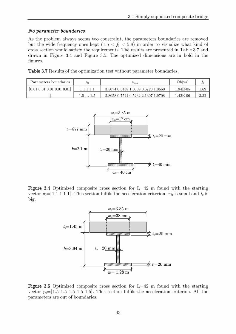
3.1 Simply supported composite bridge
43
No parameter boundaries
As the problem always seems too constraint, the parameters boundaries are removed but the wide frequency ones kept (1.5 < f0 < 5.8) in order to visualize what kind of cross section would satisfy the requirements. The results are presented in Table 3.7 and drawn in Figure 3.4 and Figure 3.5. The optimized dimensions are in bold in the figures.
Table 3.7 Results of the optimization test without parameter boundaries.
Parameters boundaries p0 pfinal Objval f0
[0.01 0.01 0.01 0.01 0.01] 1 1 1 1 1 3.5074 0.3438 1.0009 0.6723 1.0660 1.94E-05 1.69
[] 1.5 … 1.5 5.8058 0.7524 0.5232 2.1307 1.9708 1.42E-06 3.32
Figure 3.4 Optimized composite cross section for L=42 m found with the starting vector p0=[1 1 1 1 1]. This section fulfils the acceleration criterion. wu is small and tc is big.
Figure 3.5 Optimized composite cross section for L=42 m found with the starting vector p0=[1.5 1.5 1.5 1.5 1.5]. This section fulfils the acceleration criterion. All the parameters are out of boundaries.

CHAPTER 3 ANALYSIS AND RESULTS
44
Bridge with span length of 25 m
Initial boundaries
The same analysis is started again with a 25 m span, keeping the same updating parameters boundaries as the one used for the 42 m span. As a smaller bridge requires smaller stiffness, cross section area and mass, it may find a feasible solution. The first natural frequency boundaries are taken in the Eurocode: 3.51 < f0 < 8.53 Hz. Result of the optimization is presented in Table 3.8.
Table 3.8 Results of the optimization test with realistic boundaries. lb is the lower parameters boundaries vector. ub is the upper parameters boundaries vector.
Parameters boundaries p0 pfinal amax f0 STOP
lb=[0.8 0.8 0.75 0.6 0.75] 1 1 1 1 1 1.4000 1.0070 1.0038 1.0051 0.9852 18.3745 4.78
Converged to incorrect value ub=[1.4 1.2 1.25 1.3 1.5]
Once again, the problem does not have any solution. The boundaries constrain too much the model to be able to match realistic frequencies and correct vertical acceleration.
No parameters boundaries
The parameters boundaries are removed but the natural frequency boundaries are kept identical. The results are presented in Table 3.9 and drawn in Figure 3.6, Figure 3.7 and Figure 3.8. The optimized dimensions are in bold in the figures.
Table 3.9 Results of the optimization test without parameter boundaries.
Boundaries p0 pfinal Objval f0
[] 1 1 1 1 1 1.7425 0.7241 0.4530 1.0152 1.9211 9.70E-07 8.51
[] 1.5 1.5 1.5 1.5 1.5 1.6419 1.5430 1.3884 1.4781 1.4764 1.87E-06 8.52
[0.01 … 0.01] 0.6 0.6 0.6 0.6 0.6 1.7647 0.0106 0.6564 0.6405 1.9428 2.00E-05 8.52
[]

3.1 Simply supported composite bridge
45
Figure 3.6 Optimized composite cross section for L=25 m found with the starting vector p0=[1 1 1 1 1]. This section fulfils the acceleration criterion.
Figure 3.7 Optimized composite cross section for L=25 m found with the starting vector p0=[1.5 1.5 1.5 1.5 1.5]. This section fulfils the acceleration criterion.
Figure 3.8 Optimized composite cross section for L=25 m found with the starting vector p0=[0.6 0.6 0.6 0.6 0.6]. This section fulfils the acceleration criterion.

CHAPTER 3 ANALYSIS AND RESULTS
46
3.1.5 Optimization of the height of the steel beam
As varying all parameters of the cross section do not give usable results, in this section, only the height of the steel beam is optimized. The thickness of all flanges are fixed to 20 mm and their width to 40 cm. The dimensions are presented in Figure 3.9.
Figure 3.9 Composite cross section (half).
In Figure 3.10, the maximum vertical deck acceleration is plotted as a function of the steel beam height for several span lengths. In Figure 3.11, the beam height is plotted against the span length for bridges that satisfy the maximum vertical deck acceleration criterion. The maximum vertical acceleration is more or less sensitive to the height of the steel beam, depending on the span length. When the acceleration is sensitive, the corresponding height of the beam is represented by a circle in Figure 3.11. When it is not and a range of heights gives satisfying maximum vertical deck acceleration, the heights are represented by vertical lines. The higher values of the height per span length are linked together to give a curve of the beam height against span length for solutions which satisfy the acceleration criterion (on the safe side). In Figure 3.11, points in grey represent bridges that satisfy the maximum vertical deck acceleration criterion but with a first natural frequency out of the boundaries presented in the Eurocode.

3.1 Simply supported composite bridge
47
Figure 3.10 Absolute vertical acceleration as a function of the steel beam height h, for span length from 10 to 45 m. For a composite simply supported bridge.
Figure 3.11 Steel beam height against the span length for the bridges that satisfy the maximum acceleration criterion. For a composite simply supported bridge. The grey points/lines correspond to bridges out of the frequency zone defined in the Eurocode.
1 2 3 4 5 6 70
0.5
1
1.5
2
2.5
3
3.5
4
4.5
5
h (m)
Maxim
um
vert
ical accele
ration (
m/s
^2)
.
L=10 m
L=15 m
L=20 m
L=25 m
L=30 m
L=35 m
L=40 m
L=45 m
3,5 m/s2
5 10 15 20 25 30 35 40 45 500
1
2
3
4
5
6
7
L, Span length (m)
h,
Beam
heig
ht
(m)

CHAPTER 3 ANALYSIS AND RESULTS
48
The steel beam height varies up to 7 m, which is very high as the beam height usually does not exceed 3.5 m. For span length between 20 and 30 m, the maximum vertical acceleration is very sensitive to the steel beam height. Besides, in this range, the only height for which 3.5 m/s2 is satisfied corresponds to a bridge with a high first natural frequency (higher than the boundaries defined in the Eurocode). Only the values for 10 and 15 m span seem to be reasonable. This confirms what was pointed out previously: composite bridges between 20 and 45 m are not suitable for high-speed lines if it is admitted that the first natural frequency has to be situated in the boundaries defined by the Eurocode. However, reasonable dimensions might be possible to find for bridges up to 25 m long, by increasing the flange dimensions, etc.
3.2 Optimization of a prestressed concrete bridge section
Many combinations of I and M can give satisfactory results regarding the maximum vertical acceleration and the first natural frequency for a prestressed concrete simply supported bridge. Consequently, optimization functions cannot be used as it finds only one of the solutions. All combinations of parameters have to be calculated to identify the zone where the adequate combinations are. A 29 m existing bridge situated in Norrmjöleån is taken as reference to determine the frame values of the updating parameters. I is decided to be varied between 1 and 4 m4. M is deduced from I and f0.
Table 3.10 Input data used for the study.
Input data
L 29 m
E 35 GPa
I 1 < I < 4 m4
M 2275 < M < 51391 kg/m
material prestressed concrete
The values of the objective function are calculated as in the section 2.4.5. Acceleration between 3.3 and 3.7 m/s2 are accepted. The satisfying combinations are shown in Table 3.11. The minimum is found for I=3.91 m4 and M=23582.33 kg/m. Nevertheless, if lower values of I and M are wished, I=3.41 m4 and M=19047 kg/m are found to be suitable parameter combination as well. In Figure 3.12, the whole scanned area is plotted and the suitable minima, corresponding to the values presented in Table 3.11, are hatched. The same procedure can be used for any span length of concrete bridges in order to find the optimized parameters.

3.2 Optimization of a prestressed concrete bridge section
49
Figure 3.12 Objective function value as a function of I and M.
Table 3.11 Suitable parameter combinations for a 29 m prestressed concrete simply supported bridge. Values corresponding to the hatched zone in Figure 3.12.
I M Objval f0
3.41 19047 -5.42E-02 4.68
3.44 19047 -2.59E-02 4.70
3.47 19047 -4.66E-02 4.72
3.57 19047 -5.59E-02 4.78
3.60 19047 -3.20E-02 4.80
3.63 19047 -3.91E-02 4.82
3.75 19047 -4.62E-02 4.90
3.78 19047 -1.79E-02 4.92
3.81 19047 -4.97E-02 4.94
3.94 19047 -4.41E-02 5.02
3.97 19047 -1.87E-02 5.04
4.00 19047 -4.85E-02 5.06
3.50 19954 -1.62E-02 4.63
3.53 19954 -2.02E-02 4.65
3.57 19954 -9.63E-03 4.67
3.60 19954 1.15E-02 4.69
(cont. on next page)
0.015
0.015
0.015
0.015
0.0150.015
0.015
0.06
0.06
0.06
0.06
0.060.06
0.06
0.06
0.060.2
0.2
0.2
0.2
0.20.2
0.2
0.2
0.2
0.2 0.20.4
0.4
0.4
0.4
0.4
0.40.4
0.4
0.4
0.4 0.4
0.6
0.6
0.6
0.6
0.6
0.6
0.6
0.6
0.6
0.6 0.60.6
1
1
1
1
1
1
111
1
1
1
11
2
2
2
22
2 2
2
2
3
3
3
33
3
5
5
5
6
6
Second moment of inertia I (m4)
Cro
ss s
ection m
ass M
(kg/m
)
2 2.5 3 3.5 4 4.5 5 5.5 6
0.5
1
1.5
2
2.5

CHAPTER 3 ANALYSIS AND RESULTS
50
I M Objval f0
3.63 19954 1.10E-02 4.71
3.66 19954 -1.34E-02 4.73
3.69 19954 -2.10E-02 4.75
3.72 19954 -1.25E-02 4.77
3.75 19954 1.37E-03 4.79
3.78 19954 2.74E-02 4.81
3.81 19954 -3.08E-03 4.83
3.84 19954 -1.86E-02 4.85
3.88 19954 -1.97E-02 4.87
3.91 19954 -1.01E-02 4.89
3.94 19954 6.57E-03 4.91
3.97 19954 2.18E-02 4.93
4.00 19954 -4.99E-03 4.95
3.69 20861 2.35E-02 4.65
3.72 20861 3.22E-02 4.67
3.75 20861 4.75E-02 4.69
3.81 20861 3.69E-02 4.72
3.84 20861 2.44E-02 4.74
3.88 20861 2.62E-02 4.76
3.91 20861 3.65E-02 4.78
3.94 20861 5.64E-02 4.80
3.97 20861 5.53E-02 4.82
4.00 20861 3.30E-02 4.84
3.75 22675 -4.00E-02 4.49
3.78 22675 -4.88E-02 4.51
3.81 22675 -5.39E-02 4.53
3.84 22675 -5.47E-02 4.55
3.88 22675 -5.13E-02 4.57
3.91 22675 -4.39E-02 4.59
3.94 22675 -3.28E-02 4.60
3.97 22675 -2.13E-02 4.62
3.91 23582 -8.97E-04 4.50
3.94 23582 -9.24E-03 4.51
3.97 23582 -1.36E-02 4.53
4.00 23582 -1.41E-02 4.55

3.3 Concrete U-section simply supported bridge
51
3.3 Concrete U-section simply supported bridge
In this section, a concrete open section simply supported bridge has been investigated. The height of the edge beam is the only updating parameter. Dimensions of the bridge are presented in Figure 3.13. The bridge is 7 m wide, the edge beams are 1.2 m wide and the slab 0.5 m thick. The ballast is 0.6 m thick. The program to create the input parameters of the open section is presented in Appendix E.
Figure 3.13 Open section of a simply supported concrete bridge.
The height of the edge beam is varied between 1.1 and 6.0 m. The maximum vertical acceleration is calculated as a function of the beam height for span lengths of 10 to 40 m. The maximum vertical acceleration is more or less sensitive to the height of the beam, depending on the span length. Results are presented from Figure 3.14 to Figure 3.20. When the acceleration is sensitive to the height of the beam, the corresponding height is represented by a circle. When it is not and a range of heights gives satisfying maximum vertical deck acceleration, the heights are represented by vertical lines. The higher values of the height per span length are linked together to give a curve of the beam height against span length for solution which satisfy the acceleration criterion (on the safe side). Points in grey represent bridge having a first natural frequency out of the boundaries presented in the Eurocode. Accelerations are considered as acceptable between 3.3 m/s2 and 3.7 m/s2.
The prestressed bridge alternative differs from the ordinary concrete bridge regarding the damping ratio and the E-modulus. Cracking of ordinary concrete is considered in this structure by reduction of E.
Results for a prestressed concrete bridge are presented in Figure 3.14 and Figure 3.15. Results for an ordinary concrete bridge are presented in Figure 3.16 and Figure 3.17. Results for an ordinary concrete ballastless bridge are presented in Figure 3.18 and Figure 3.19.

CHAPTER 3 ANALYSIS AND RESULTS
52
3.3.1 Prestressed concrete ballasted bridge
Figure 3.14 Absolute vertical acceleration as a function of the beam height h, for span length from 10 to 40 m. For a prestressed concrete simply supported bridge.
Figure 3.15 Beam height against the span length for the bridges that satisfy the maximum acceleration criterion. For a prestressed concrete simply supported bridge.
1 1.5 2 2.5 3 3.5 4 4.5 5 5.50
0.5
1
1.5
2
2.5
3
3.5
4
4.5
5
h (m)
Maxim
um
vert
ical accele
ration (
m/s
2)
L=10 m
L=15 m
L=20 m
L=25 m
L=30 m
L=35 m
L=40 m
3,5 m/s2
5 10 15 20 25 30 35 40 450
0.5
1
1.5
2
2.5
3
3.5
4
L, Span length (m)
h,
Beam
heig
ht
(m)
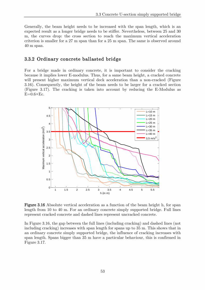
3.3 Concrete U-section simply supported bridge
53
Generally, the beam height needs to be increased with the span length, which is an expected result as a longer bridge needs to be stiffer. Nevertheless, between 25 and 30 m, the curves drop: the cross section to reach the maximum vertical acceleration criterion is smaller for a 27 m span than for a 25 m span. The same is observed around 40 m span.
3.3.2 Ordinary concrete ballasted bridge
For a bridge made in ordinary concrete, it is important to consider the cracking because it implies lower E-modulus. Thus, for a same beam height, a cracked concrete will present higher maximum vertical deck acceleration than a non-cracked (Figure 3.16). Consequently, the height of the beam needs to be larger for a cracked section (Figure 3.17). The cracking is taken into account by reducing the E-Modulus as E=0.6×Ec.
Figure 3.16 Absolute vertical acceleration as a function of the beam height h, for span length from 10 to 40 m. For an ordinary concrete simply supported bridge. Full lines represent cracked concrete and dashed lines represent uncracked concrete.
In Figure 3.16, the gap between the full lines (including cracking) and dashed lines (not including cracking) increases with span length for spans up to 35 m. This shows that in an ordinary concrete simply supported bridge, the influence of cracking increases with span length. Spans bigger than 35 m have a particular behaviour, this is confirmed in Figure 3.17.
1 1.5 2 2.5 3 3.5 4 4.5 5 5.50
0.5
1
1.5
2
2.5
3
3.5
4
4.5
5
h (in m)
Maxim
um
vert
ical accele
ration (
m/s
2)
L=10 m
L=15 m
L=20 m
L=25 m
L=30 m
L=35 m
L=40 m
3,5 m/s2
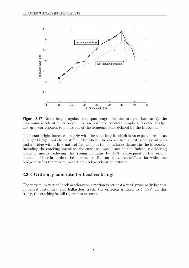
CHAPTER 3 ANALYSIS AND RESULTS
54
Figure 3.17 Beam height against the span length for the bridges that satisfy the maximum acceleration criterion. For an ordinary concrete simply supported bridge. The grey corresponds to points out of the frequency zone defined by the Eurocode.
The beam height increases linearly with the span length, which is an expected result as a longer bridge needs to be stiffer. After 35 m, the curves drop and it is not possible to find a bridge with a first natural frequency in the boundaries defined in the Eurocode. Including the cracking translates the curve to upper beam height. Indeed, considering cracking means reducing the Young modulus by 40%, consequently, the second moment of inertia needs to be increased to find an equivalent stiffness for which the bridge satisfies the maximum vertical deck acceleration criterion.
3.3.3 Ordinary concrete ballastless bridge
The maximum vertical deck acceleration criterion is set at 3.5 m/s2 principally because of ballast instability. For ballastless track, the criterion is fixed to 5 m/s2. In this study, the cracking is still taken into account.
5 10 15 20 25 30 35 40 450
0.5
1
1.5
2
2.5
3
3.5
L, Span length (m)
h,
Beam
heig
ht
(m)
Not including cracking
Including cracking

3.3 Concrete U-section simply supported bridge
55
Figure 3.18 Absolute vertical acceleration as a function of the beam height h, for span length from 10 to 40 m. For an ordinary concrete ballastless simply supported bridge, considering cracking.
Figure 3.19 Beam height against the span length for the bridges that satisfy the maximum acceleration criterion. For an ordinary concrete ballastless simply supported bridge, considering cracking. The grey corresponds to points out of the frequency zone defined by the Eurocode.
1 1.5 2 2.5 3 3.5 4 4.5 5 5.50
1
2
3
4
5
6
h (m)
Maxim
um
vert
ical accele
ration (
m/s
2)
L=10 m
L=15 m
L=20 m
L=25 m
L=30 m
L=35 m
L=40 m
5 m/s2
5 10 15 20 25 30 35 40 450
0.5
1
1.5
2
2.5
3
3.5
L, Span length (m)
h,
Beam
heig
ht
(m)

CHAPTER 3 ANALYSIS AND RESULTS
56
The same conclusion as before can be drawn: the beam height increases linearly with the span length, which is an expected result as a longer bridge needs to be stiffer. After 35 m, the curves drop and it is not possible to find a bridge with a first natural frequency in the boundaries defined in the Eurocode.
3.3.4 Comparison between ballasted and ballastless track
Ballasted tracks require higher beam height than ballastless ones. Indeed, ballasted tracks need to be stiffer and to vibrate less to avoid problem of ballast instability. It can be noticed that the two curves representing the absolute vertical acceleration against the beam height (Figure 3.16 and Figure 3.18) are the same. The ballastless plot is a translation of the ballasted one to higher values (from 3.5 m/s2 to 5 m/s2). This is confirmed by the Figure 3.20, the required beam height for a ballasted track is a translation of the ballastless one.
Figure 3.20 Beam height h against span length L. Comparison of ballasted and ballastless track.
3.3.5 Sensibility of the results
The figures presenting the height of the beam against the span length have to be used with precaution. Circles (Figure 3.15, Figure 3.17 and Figure 3.19) represent values extremely sensitive to a small variation of the beam height.
As an example, an ordinary concrete 10 m span open section with ballast is taken, without including the cracking. The vertical acceleration criterion is satisfied for h=0.96 m. For that value, the maximum vertical acceleration is 2.9079 m/s2, which
5 10 15 20 25 30 35 40 450
0.5
1
1.5
2
2.5
3
3.5
L, Span length (m)
h,
Beam
heig
ht
(m) ballastless
ballasted

3.3 Concrete U-section simply supported bridge
57
occurs at 150 km/h under the HLSM-A2 train. If, instead, h=0.95 m, the maximum vertical acceleration is 4.4180 m/s2, which occurs at 350 km/h under the HSLM-A7 train. Both maximum accelerations occur at the node 36 (the beam is divided into 70 elements), that is to say at mid-span. The bridge response as a function of time is plotted for these two cases in Figure 3.21. In Figure 3.22, the acceleration as function of the speed is plotted for the two bridges studied. It is found that increasing the beam height shifts the acceleration peak out of the investigated speeds.
It should be noted that λ (=v/f0) is the analysis step in the signature analysis. Consequently, it depends on the bridge first natural frequency. Besides, it can be seen in Figure 3.22 that both bridges (h=0.95 m and h=0.96 m) exceeds 3.5 m/s2 before 350 km/h, but the acceleration is calculated just before 350 km/h for the bridge h=0.95 m whereas it is calculated just after for the bridge h=0.96 m. The accelerations for both bridges should have been computed at 350 km/h. The study should have been carried out for a fixed sampling speed, similar for all bridges, which is not the case in this work. As a result, an error is introduced around 350 km/h. Consequently, the work presented before is only valid for speeds up to 340 km/h.
Figure 3.21 Vertical acceleration against time at mid-span (node 36). Top: h=0.95 m, HSLM-A7 running at 350 km/h. Botton: h=0.96m, HSLM-A2 running at 150 km/h.
0 0.5 1 1.5 2 2.5 3 3.5 4-6
-4
-2
0
2
4
6
Time (s)
Vert
ical accele
ration (
m/s
2)
h=0.95 m. HSLMA-7. 350 km/h
0 1 2 3 4 5 6 7 8 9-6
-4
-2
0
2
4
6
Time (s)
Vert
ical accele
ration (
m/s
2)
h=0.96 m. HSLMA-2. 150 km/h
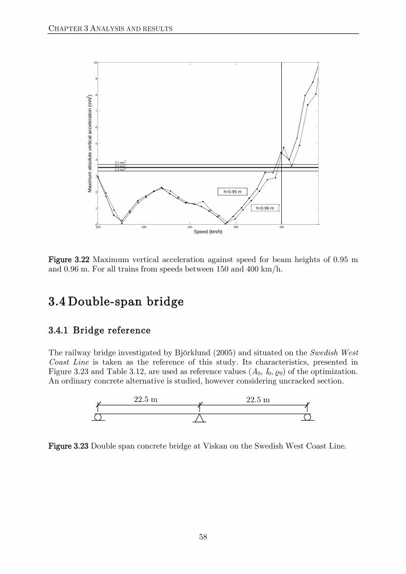
CHAPTER 3 ANALYSIS AND RESULTS
58
Figure 3.22 Maximum vertical acceleration against speed for beam heights of 0.95 m and 0.96 m. For all trains from speeds between 150 and 400 km/h.
3.4 Double-span bridge
3.4.1 Bridge reference
The railway bridge investigated by Björklund (2005) and situated on the Swedish West Coast Line is taken as the reference of this study. Its characteristics, presented in Figure 3.23 and Table 3.12, are used as reference values (A0, I0, ρ0) of the optimization. An ordinary concrete alternative is studied, however considering uncracked section.
Figure 3.23 Double span concrete bridge at Viskan on the Swedish West Coast Line.
150 200 250 300 3500
1
2
3
4
5
6
7
8
9
10
Speed (km/h)
Maxim
um
absolu
te v
ert
ical accele
ration (
m/s
2)
3.5 m/s23.7 m/s2
h=0.96 m
h=0.95 m
3.3 m/s2
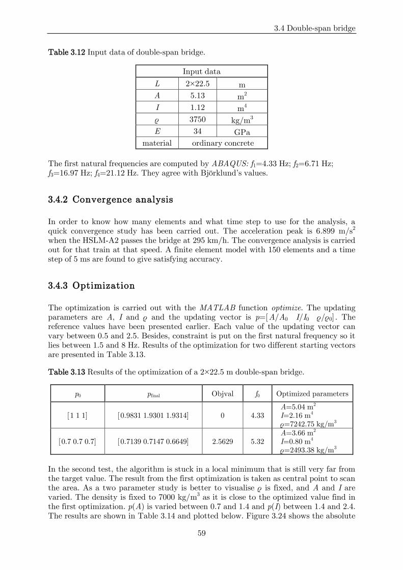
3.4 Double-span bridge
59
Table 3.12 Input data of double-span bridge.
Input data
L 2×22.5 m
A 5.13 m2
I 1.12 m4
ρ 3750 kg/m3
E 34 GPa
material ordinary concrete
The first natural frequencies are computed by ABAQUS: f1=4.33 Hz; f2=6.71 Hz; f3=16.97 Hz; f4=21.12 Hz. They agree with Björklund’s values.
3.4.2 Convergence analysis
In order to know how many elements and what time step to use for the analysis, a quick convergence study has been carried out. The acceleration peak is 6.899 m/s2 when the HSLM-A2 passes the bridge at 295 km/h. The convergence analysis is carried out for that train at that speed. A finite element model with 150 elements and a time step of 5 ms are found to give satisfying accuracy.
3.4.3 Optimization
The optimization is carried out with the MATLAB function optimize. The updating parameters are A, I and ρ and the updating vector is p=[A/A0 I/I0 ρ/ρ0]. The reference values have been presented earlier. Each value of the updating vector can vary between 0.5 and 2.5. Besides, constraint is put on the first natural frequency so it lies between 1.5 and 8 Hz. Results of the optimization for two different starting vectors are presented in Table 3.13.
Table 3.13 Results of the optimization of a 2×22.5 m double-span bridge.
p0 pfinal Objval f0 Optimized parameters
[1 1 1] [0.9831 1.9301 1.9314] 0 4.33 A=5.04 m2 I=2.16 m4 ρ=7242.75 kg/m3
[0.7 0.7 0.7] [0.7139 0.7147 0.6649] 2.5629 5.32 A=3.66 m2 I=0.80 m4 ρ=2493.38 kg/m3
In the second test, the algorithm is stuck in a local minimum that is still very far from the target value. The result from the first optimization is taken as central point to scan the area. As a two parameter study is better to visualise ρ is fixed, and A and I are varied. The density is fixed to 7000 kg/m3 as it is close to the optimized value find in the first optimization. p(A) is varied between 0.7 and 1.4 and p(I) between 1.4 and 2.4. The results are shown in Table 3.14 and plotted below. Figure 3.24 shows the absolute

CHAPTER 3 ANALYSIS AND RESULTS
60
maximum vertical acceleration as a function of A and I (values in Table 3.14). Figure 3.25 and Figure 3.26 present the objective function values as a function of the area and the second moment of inertia. The first natural frequency has been quickly checked but has not been considered as a limiting factor in this study.
Table 3.14 Absolute vertical acceleration as a function of A and I.
amax p(A)=0.7 p(A)=0.8 p(A)=0.9 p(A)=1.0 p(A)=1.1 p(A)=1.2 p(A)=1.3 p(A)=1.4
A=3.591 A=4.104 A=4.617 A=5.130 A=5.643 A=6.156 A=6.669 A=7.182
p(I)=1.4 I=1.568 5.047 4.492 4.118 5.587 6.219 5.694 5.423 4.959
p(I)=1.6 I=1.792 4.989 4.416 4.040 3.558 4.374 5.395 5.373 5.030
p(I)=1.8 I=2.016 5.009 4.571 3.926 3.704 3.186 3.156 4.292 4.964
p(I)=2.0 I=2.240 4.896 4.624 4.155 3.533 3.390 3.086 2.817 3.798
p(I)=2.2 I=2.464 3.549 4.251 3.892 3.704 3.212 3.070 2.870 2.663
p(I)=2.4 I=2.688 2.595 4.417 4.152 3.642 3.314 2.944 2.753 2.589
p(I)=2.6 I=2.912 2.569 2.346 3.548 3.490 3.402 2.983 2.718 2.516
Figure 3.24 Absolute vertical deck acceleration as a function of the cross section area and the second moment of inertia.
Figure 3.24 shows that the maximum vertical deck acceleration does not decrease steadily while increasing the cross section area or/and the second moment of inertia. For example, if I is kept equal to 1.792 m4, first the acceleration decreases when the area increases from 3.591 to 5.130 m2, but after that point the acceleration increases with A.
3
4
5
6
7
8
1.5
2
2.5
3
2
3
4
5
6
7
Cross section area A (m2)Second moment of inertia I (m4)
Absolu
te v
ert
ical accele
ration (
m/s
2)

3.4 Double-span bridge
61
Figure 3.25 Objective function value as a function of the cross section area and the second moment of inertia.
Figure 3.26 Objective function value as a function of the cross section area and the second moment of inertia. The grey thick lines correspond to the objective function value equal or below 0.015 (i.e maximum acceleration between 3.45 m/s2 and 3.55 m/s2). The black thick lines correspond to the objective function value equal or below 0.06 (i.e maximum acceleration between 3.3 m/s2 and 3.7 m/s2).
3.54
4.55
5.56
6.57
7.5
1.5
2
2.5
3
0
0.2
0.4
0.6
0.8
Cross section area A (m2)
Second moment of inertia I (m4)
Obje
ctive f
unction
Cross section area A (m2)
Second m
om
ent
of
inert
ia I
(m
4)
0.06
0.0
6
0.0
6
0.06
0.06
0.0
6
0.015
4 4.5 5 5.5 6 6.5 7
1.6
1.8
2
2.2
2.4
2.6
2.8
CHAPTER 3 ANALYSIS AND RESULTS
62
The global minimum (thick grey line) is situated around A=5.3 m2 and I=2.25 m4, which corresponds to the parameters found by the first optimization test (starting values [1 1 1]).
To build a concrete double-span 2×22.5 m bridge that has a maximum vertical deck acceleration between 3.3 and 3.7 m/s2, possible parameter combinations can be read inside the thick black line in Figure 3.26. Nevertheless, the scanned area should be widened to the left as the thick black line around [3.6 2.5] suggests the presence of other suitable minima.
3.4.4 Optimization of a concrete 60 m double span bridge
The same study is carried out on a 2×30 m double-span bridge. It is assumed that 151 elements and a time step of 5 ms can be applied here as well. A quick convergence study has been carried out and confirmed the hypothesis. All the reference parameters are kept the same and the study parameters as well.
In the optimization process, the upper boundaries are widened to 3 (previously 2.5). The result of the optimization is presented Table 3.15.
Table 3.15 Results of the optimization of a 2×30 m double-span bridge.
p0 pfinal Objval f0 Optimized parameters
[1.5 1.5 1.5] [1.9784 2.0869 1.5707] 0 2.00 A=10.15 m2 I=2.34 m4 ρ=5890.13 kg/m3
As previously, the result of the optimization is taken as central point to scan the area acceleration. A and I are varied and ρ kept fixed at 7000 kg/m3.
To build a concrete double-span 2×30 m bridge that has a maximum vertical deck acceleration between 3.3 and 3.7 m/s2, possible parameter combinations can be read inside the thick black line in Figure 3.27.

3.4 Double-span bridge
63
Figure 3.27 Objective function value as a function of the cross section area and the second moment of inertia. The grey thick lines correspond to the objective function value equal or below 0.015 (i.e maximum acceleration between 3.45 m/s2 and 3.55 m/s2). The black thick lines correspond to the objective function value equal or below 0.06 (i.e maximum acceleration between 3.3 m/s2 and 3.7 m/s2).
Cross section area A (m2)
Second m
om
ent
of
inert
ia I
(m
4)
0.06
0.06
0.0
6
0.060.06
0.06
0.0
15
0.0
15
7.5 8 8.5 9 9.5 10 10.5 11
1.5
2
2.5
3
3.5


4.1 Analysis method
65
Chapter 4 Conclusions and suggestions for future work
Finding bridge parameters that satisfy the maximum vertical acceleration criterion defined in the Eurocode for railway bridges is the daily challenge of designers. Optimizing the research of the optimized parameters is a new subject this master thesis started to investigate. Conclusions about the method to use for this purpose and about the results are presented below. Hints for further researches are also given.
4.1 Analysis method
(i) Investigations showed that there exists not just one set of optimized parameters satisfying the maximum vertical deck acceleration criterion but several. However, MATLAB optimization algorithm finds one of them and stops. If all the combinations of suitable parameters want to be found, the optimization algorithm should not be used. Instead, parameters should be varied in a well-defined range and the maximum acceleration computed for each parameter combination. Only upon scanning this area can the suitable parameters be picked up. Nevertheless, the optimization algorithms can be used to determine in what area(s) the minima are situated. In that case, the algorithm has to be run from several starting values. The procedure to find optimized bridge parameters is detailed in section 2.4.6.
(ii) On the contrary, when no minimum is found, before questioning the program and re-doing all the analysis in a different way, which is very time consuming, a test should be made on an existing bridge that actually satisfies the criteria defined in the optimization. It has to be considered that the optimization problem might not have any solution (as it is the case for a 42 m composite bridge studied herein).
(iii) Whatever the results are, every analysis takes a lot of time. On one hand, the optimization algorithm makes many iterations before converging and ending. On the other hand, depending on the computation method, determining the maximum vertical deck acceleration can be very time consuming. Therefore, it is important to think about clever starting

CHAPTER 4 CONCLUSIONS AND SUGGESTIONS FOR FUTURE WORK
66
parameters in order to find a suitable minimum as fast as possible. Besides, minimizing ABAQUS analysis time is a serious topic.
(iv) If possible, it is preferable to run one-parameter or two-parameter studies as this is easier to visualize and understand. A study with more parameters is hard to present in a convenient way (on a graph).
4.2 Results
The study is made on single-track railway bridges and the following conclusion can be drawn:
(i) Simply supported composite bridges with span larger than 20 m are not suitable for high-speed railways when considering the maximum vertical deck acceleration criterion and the first frequency boundaries defined in the Eurocode.
(ii) The optimized parameters of a 29 m prestressed concrete simply supported bridge are presented in Table 3.11.
(iii) Optimal height of an open section of concrete simply supported bridges from 10 to 40 m was found and presented in Figure 3.15, Figure 3.17 and Figure 3.19.
(iv) Open section concrete simply supported bridges without ballast need a smaller beam height than ballasted ones (Figure 3.20).
(v) For spans over 35 m, ordinary concrete simply supported bridges cannot respect both the dynamic criterion and the first natural frequency boundaries defined in the Eurocode.
(vi) The optimized parameters of reinforced concrete double-span bridges 2×22.5 m and 2×30 m are respectively presented in Figure 3.26 and Figure 3.27.
4.3 Limits
In this work, bridges have been tested from 150 km/h to 350 km/h. Nevertheless, it might sometimes be necessary to check a wider speed interval. Indeed, it has been shown that the first resonance speed can be calculated with v=f0×λ. The smallest axle distance of HSLM-A trains is 18 m and the lowest first natural frequency considered in this work is 1.5 Hz. Consequently, the lowest possible resonance speed is at v=1.5×18=27 m/s =97.2 km/h. When the first natural frequency boundaries were widened to 1.5 Hz, the speed interval investigated should have been widened as well.
However, in most cases, the first natural frequency has been limited to the boundaries defined in the Eurocode (see Figure 2.21) and the longest bridge investigated here was 45 m. In Figure 2.21, the lowest frequency of a 45 m span bridge is 2.48 Hz. For this

4.4 Further research
67
frequency, which is the lowest for a bridge considered realistic in this study, the resonance speed is v=2.48×18=44.64 m/s=160.7 km/h. Consequently, as long as the first natural frequencies are taken as the boundaries defined by the Eurocode, the checked speed interval (150 to 350 km/h) is sufficient.
4.4 Further research
(i) The investigations presented in this master thesis for single-track simply supported and double-span bridges should be extended to other types of bridges (frame bridges, three-span bridges, etc).
(ii) This master thesis has considered the first natural frequency boundaries defined in the Eurocode as a reference regarding the feasibility of the bridge. This constraint should be removed. Instead, a static analysis should be first carried out in order to determine the minimum values of the cross section parameters for the bridge to satisfy the static criteria. The latter values should be then taken as low boundaries in the optimization process. Thus, all parameter combinations tried in the optimization would correspond to realistic bridges.
(iii) Another criterion should be added to the optimization process in order to limit the number of minima. Thus, tables of optimized parameters could be created: for example, one table presenting the optimized parameters of a given type of bridge if the dynamic criterion and the cost of the structure are considered, another table considering the dynamic criterion and the Life Cycle Cost, etc. Besides, the tolerance on the maximum vertical deck acceleration and the parameters boundaries should be well defined from the beginning and kept fixed all along the study.
(iv) ABAQUS analysis time needs to be optimized; the suggestions in the concerned section should be investigated. The optimization loop should also be optimized. For example by creating a shortcut in the speed loop: as soon as an acceleration higher than 3.5 m/s2 is found, the loop should exit instead of trying all the following train speeds.
(v) It has to be noted that the study has been carried out for constant sections. An alternative to find composite bridges satisfying the criteria is to vary the section parameters along the beam, which is usually the case.
(vi) The performance-based optimization method described by Liang and Steven (2002) should be tested for optimizing bridges regarding the maximum vertical deck acceleration criterion.


BIBLIOGRAPHY
69
Bibliography
ABAQUS Online Documentation: Version 6.8 (2008). http://abqdoc.byv.kth.se:2080/v6.8/
Akiyama, H., Fukada, S., & Kajikawa, Y. (2007). Numerical Study on the Vibrational Serviceability of Flexible Single Span Bridges with different Structural Systems under Traffic Load. Structural Engineering International, 3, 256-263.
Bucknall, I. (2003). New Eurocode Requirements for the Design of High Speed Railway Bridges. In Structures for High-Speed Railway Transportation, IABSE Symposium, Antwerp, Belgium, August, Volume 87.
Björklund, L. (2005). Dynamic Analysis of a Railway Bridge. (Master Thesis, Royal Institute of Technology (KTH)).
Coleman, T.F. & Zhang, Y. (2009). Opimization Toolbox TM4 User’s Guide. The MathWorks, Inc.
ERRI D214 (1999). Rail bridges for speeds > 200 km/h. European Rail Research Institute (ERRI). D214/RP9 & RP3, Final report.
Eurocode (2002). Eurocode 1: actions on structures - Part 2: Traffic loads on bridges. (prEN 1991-2). European Committee for Standardization, Brussels.
Eurocode (2004). Eurocode-Basis of structural design. (EN 1990:2002 prA1). European Committee for Standardization, Brussels.
Flemming, L., Hasselberg, P., & Gillesén, C. (2000). Integration of CAD, FEM and optimization in practice. (Master thesis, Chalmers).
Friswell, M.I., & Mottershead, J.E. (1995). Finite Element Model Updating in Structural Dynamics. Dordrecht, the Netherlands: Kluwer Academic Publishers.
Frýba, L. (1996). Dynamics of Railway Bridges. London, UK: Thomas Telford.
Goicolea, J. M. (2007). Railway bridges for High Speed Lines: Dynamic Behaviour and Risk. (Master Thesis, Technical University of Madrid).
Heiden, M., Bokan, H., Simões da Silva, L., Greiner, R., Pircher, M., & Pircher, H. (2003). Dynamic effects of railway bridges for high speed usage: application example steel-composite truss bridge. Fourth congress of steel and composite construction, Lisbon.

BIBLIOGRAPHY
70
Jaishi, B., & Ren, W. (2007). Finite element model updating based on eigenvalue and strain energy residuals multiobjective optimisation technique. Mechanical Systems and Signal Processing, 21, 2295-2317.
Jonsson, F., & Johnson, D. (2007). Finite Element Model Updating of the New Svinesund Bridge. Manual Model Refinement with Non-Linera Optimization. (Master thesis, Chalmers).
Karoumi, R., & Wiberg, J. (2006). Kontrol av dynamiska effekter av passerande tåg på Botniabanans broar – Sammanfattning, (Technical Report 97). Stockholm: Royal Institute of Technology (KTH),Structural Design and Bridges.
Karoumi, R. (1998). Response of Cable-Stayed and Suspension Bridges to Moving Vehicles. Analysis methods and practical modelling techniques. (Doctoral Thesis, Royal Institute of Technology(KTH)).
Liang, Q.Q., & Steven, G.P. (2002). A performance-based optimization method for topology design of continuum structures with mean compliance constraints. Computer Methods in Applied Mechanics and Engineering, 191, 1471–1489.
Liu, K., De Roeck, G., & Lombaert, G. (2009). The effect of dynamic train-bridge interaction on the bridge response during a train passage. Journal of Sound and Vibration, 325, 240-251.
MATLAB Central-File Exchange. Gathering of helps and programs by MATLAB users. http://www.mathworks.com/matlabcentral/fileexchange/
Mathworks. Description of MATLAB products. http://www.mathworks.com/products/
Majka, M., & Hartnett, M. (2008). Effects of speed, load and damping on the dynamic response of railway bridges and vehicles. Computers and Structures, 86, 556–572.
Menn, C. (1991). An approach to bridge design. Engineering Structures, 13, 106-112.
Norris, P., Wilkins, T., & Bucknall I. (2003). Permissible Deck Accelerations For Rail Bridge Dynamic Assessments. IABSE Report, 87.
Schlune, H. (2010). Phone interview, March.
Schlune, H., Plos, M., & Gylltoft, K. (2009). Improved bridge evaluation through finite element model updating using static and dynamic measurements. Engineering Structures, 31, 1477–1485.
Schlune, H., & Plos, M. (2008). Bridge Assessment and Maintenance based on Finite Element Structural Models and Field Measurements. (Technical Report 2008:5) Göteborg: Chalmers University of Technology, Division of Structural Engineering Concrete Structures.
Wiberg, J. (2009). Railway bridge response to passing trains. Measurements and FE model updating. (Doctoral Thesis, Royal Institute of Technology (KTH)).

BIBLIOGRAPHY
71
Xia, H., De Roeck, G., Zhang, N., & Maeck, J. (2003). Experimental analysis of a high-speed railway bridge under Thalys trains. Journal of Sound and Vibration, 268, 103-113.
Xia, H., & Zhang, N. (2005). Dynamic analysis of railway bridge under high-speed trains. Computers and Structures, 83, 1891-1901.
Xia, H., Zhang, N., & Gao, R. (2005). Experimental analysis of railway bridge under high-speed trains. Journal of Sound and Vibration, 282, 517-528.
Zhu, X. Q., & Law, S. S. (2006). Moving load identification on multi-span continuous bridges with elastic bearings. Mechanical Systems and Signal Processing, 20, 1759–1782.


APPENDIX A
73
Appendix A The optimization loop of a double-span bridge
The programs to run the optimization of double-span bridges parameters are presented in this appendix. The description of the loop is presented in the figure below. The main program is Optimization.m. The left part of the flowchart calculates the maximum vertical deck acceleration and the right part of the flowchart checks the constraints on the first natural frequency.

APPENDIX A
74
Optimization.m: The main program. Calls the optimization routine optimize. Optimize calls first the objective function (so BridgeTesting.m) and then the constraints (constraint.m). The options (number of increment, tolerance, etc) of the optimization are set here. BridgeTesting.m: Directs the creation of the model, the FE analysis and the extraction of the data. It takes as input the bridge parameters and gives back to the optimization the maximum vertical deck acceleration. Inputparameters.m: Creates bridge data (A, E, I,…) from the normalized vector produced by the optimization. CreateAbaqusBridge.m: Produces the input file to create the bridge on ABAQUS. CreateLoad.m: Creates for a certain speed a cell containing time and amplitude load vectors for each train of the HSLM-A. CreateAbaqusLoad.m: Produces the input file to create the load on ABAQUS. CreatInputFile.m: Gathers input files created by CreateAbaqusBridge.m and CreateAbaqusLoad.m to make an only input file ready to be sent to ABAQUS. RunAbaqus.m: Generates the model on ABAQUS and puts the results in a .dat file. Read_acceleration.m: Reads the .dat file and extracts all maximum and minimum acceleration at each sampling time. Then, it keeps the absolute maximum vertical acceleration. KeepAmax.m: Compares maximum acceleration from one speed to another. It keeps the maximum acceleration of all speeds. constraint.m: Calls the extraction of the first natural frequency and compares it with the boundaries. If f0 is out of boundaries, a penalty factor is sent back to the optimization. Read_naturalfrequencies.m: Extracts the first natural frequency from the result file.
A.1 Optimization.m
clc; clear all; fclose('all'); tic;
% Calls ABAQUS to execute FE analysis from vector "p" amax=@(p)BridgeTesting(p);
% Aim value of acceleration: an=3.5;
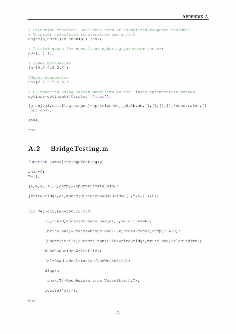
APPENDIX A
75
% Objective function: Euclidean norm of normalized response residual % Compares calculated acceleration and an=3.5 obj=@(p)norm((an-amax(p))./an);
% Initial guess for normalised updating parameter vector: p0=[1 1 1];
% Lower boundaries lb=[0.5 0.5 0.5];
%Upper boundaries ub=[2.5 2.5 2.5];
% FE updating using Nelder-Mead simplex non-linear optimization method options=optimset('Display','iter');
[p,objval,exitflag,output]=optimize(obj,p0,lb,ub,[],[],[],[],@constraint,[]
,options);
save;
toc
A.2 BridgeTesting.m
function [amax]=BridgeTesting(p)
amax=0; T=[];
[L,m,A,I11,E,damp]=Inputparameters(p);
[WriteBridge,el,modes]=CreateAbaqusBridge(L,m,A,I11,E);
for Velocitykmh=150:10:350
[v,TRAIN,Nodes]=CreateLoad(el,L,Velocitykmh);
[WriteLoad]=CreateAbaqusLoad(L,v,Nodes,modes,damp,TRAIN);
[UseWriteFile]=CreateInputFile(WriteBridge,WriteLoad,Velocitykmh);
RunAbaqus(UseWriteFile);
[a]=Read_acceleration(UseWriteFile);
disp(a)
[amax,T]=KeepAmax(a,amax,Velocitykmh,T);
fclose('all');
end
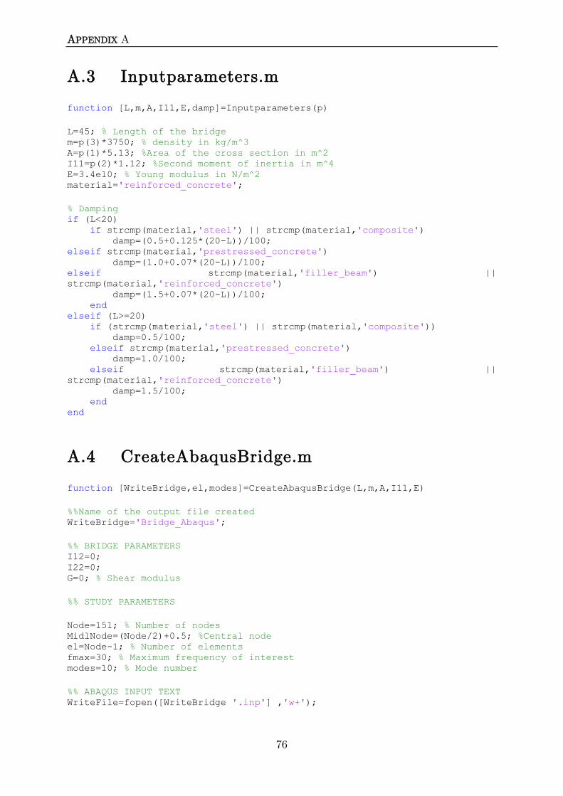
APPENDIX A
76
A.3 Inputparameters.m
function [L,m,A,I11,E,damp]=Inputparameters(p)
L=45; % Length of the bridge m=p(3)*3750; % density in kg/m^3 A=p(1)*5.13; %Area of the cross section in m^2 I11=p(2)*1.12; %Second moment of inertia in m^4 E=3.4e10; % Young modulus in N/m^2 material='reinforced_concrete';
% Damping if (L<20) if strcmp(material,'steel') || strcmp(material,'composite') damp=(0.5+0.125*(20-L))/100; elseif strcmp(material,'prestressed_concrete') damp=(1.0+0.07*(20-L))/100; elseif strcmp(material,'filler_beam') ||
strcmp(material,'reinforced_concrete')
damp=(1.5+0.07*(20-L))/100; end elseif (L>=20) if (strcmp(material,'steel') || strcmp(material,'composite')) damp=0.5/100; elseif strcmp(material,'prestressed_concrete') damp=1.0/100; elseif strcmp(material,'filler_beam') ||
strcmp(material,'reinforced_concrete') damp=1.5/100; end end
A.4 CreateAbaqusBridge.m
function [WriteBridge,el,modes]=CreateAbaqusBridge(L,m,A,I11,E)
%%Name of the output file created WriteBridge='Bridge_Abaqus';
%% BRIDGE PARAMETERS I12=0; I22=0; G=0; % Shear modulus
%% STUDY PARAMETERS
Node=151; % Number of nodes MidlNode=(Node/2)+0.5; %Central node el=Node-1; % Number of elements fmax=30; % Maximum frequency of interest modes=10; % Mode number
%% ABAQUS INPUT TEXT WriteFile=fopen([WriteBridge '.inp'] ,'w+');

APPENDIX A
77
Text=['*HEADING\n' ... '** Generated by: Abaqus/CAE Version 6.8-1\n' ... ]; fprintf(WriteFile,Text);
% Creation of the nodes Text=['*NODE\n'... '1, 0, 0\n'... num2str(Node) ',' num2str(L) ',0\n'... '*NGEN, NSET=BridgeNodes\n'... '1,' num2str(Node) ', 1\n'... ];
fprintf(WriteFile,Text);
% Creation of the elements
Text=['*ELEMENT, TYPE=B21\n'... '1, 1, 2\n'... '*ELGEN, ELSET=BEAM\n'... '1,' num2str(el) '\n'... ];
fprintf(WriteFile,Text);
% SECTION. Creation of the section Text=['*BEAM GENERAL SECTION, DENSITY=' num2str(m) ', ELSET=BEAM,
SECTION=GENERAL\n'... num2str(A) ',' num2str(I11) ',' num2str(I12) ',' num2str(I22) ', 0,
0, 0\n'... '0, 0, -1\n'... num2str(E) ',' num2str(G) '\n'... '** \n'... ];
fprintf(WriteFile,Text);
% BOUNDARY CONDITIONS Text=['*BOUNDARY\n'... '1, 2\n'... num2str(MidlNode) ', PINNED\n'... num2str(Node) ', 2\n'... '**\n'... ];
fprintf(WriteFile,Text);
% EIGENVALUE CALCULATION Text=['*STEP\n'... '*FREQUENCY\n'... num2str(modes) ', ,' num2str(fmax) '\n'... '*EL PRINT, FREQUENCY=0\n'... '*NODE PRINT, FREQUENCY=0 \n'... '*RESTART, WRITE\n'... '*END STEP\n'... ];
fprintf(WriteFile,Text);

APPENDIX A
78
A.5 CreateLoad.m
function [v,TRAIN,Nodes]=CreateLoad(el,L,Velocitykmh)
TRAIN=cell(10,1); %Cell created to store the 10 trains at once
for traintype=1:10
%% LOAD %Train speed v=Velocitykmh/3.6; % in m/s
%Call HSLMA.m [TRAINLOAD,TRAINDIST]=HSLMA(traintype);
%% NODES %Nodes vector Nodes=[]; Nodes=[0:L/el:L];
%% TIME VECTOR
% Distance between two nodes Mesh=abs(Nodes(2)-Nodes(1));
% Time before train enters bridge tbefore=-Mesh/v;
% Time when load reaches node i TIME=[]; TIME=[tbefore]; for i=1:length(Nodes)+1 ti=tbefore+i*Mesh/v; TIME=[TIME ti]; end
% Time vector for one load (one row=one moment) AMPtime=[]; for i = 2:length(TIME)-1 AMPtime = [AMPtime ; TIME(i-1) TIME(i) TIME(i+1)]; end
%Amplitude time function FOR THE WHOLE TRAIN %Creating train time vector from the distance vector "TRAINDIST" TRAINTIME=TRAINDIST/v;
AMPTIME=[]; for i=1:length(TRAINTIME) AMPTIME=[AMPTIME AMPtime+TRAINTIME(i)]; end
%% AMPLITUDE LOAD FUNCTION
%Amplitude load functions for one unit load AMPload = [zeros(size(AMPtime,1),1) ones(size(AMPtime,1),1) ...

APPENDIX A
79
zeros(size(AMPtime,1),1)];
%Amplitude load function FOR THE WHOLE TRAIN AMPLOAD=[]; for i=1:length(TRAINTIME) AMPLOAD= [AMPLOAD AMPload*TRAINLOAD(i)]; end
%% COMBINING TIME AND LOAD FUNCTION
AMP = []; for i = 1:size(AMPTIME,2)
AMP = [AMP AMPTIME(1:end,i)]; AMP = [AMP AMPLOAD(1:end,i)];
end
s = struct('AMP', AMP , 'TRAINTIME', TRAINTIME, 'AMPLOAD', AMPLOAD);
TRAIN{traintype,1}=s;
end
A.6 HSLMA.m (adapted from Prof. Raid Karoumi´s)
% ******************************************** % * HSLM-A Trains * % * type 1-10 * % * prEN 1991-2:2002 final draft (p.83) * % * Raid Karoumi 2003-12-14 * % ********************************************
function [TRAINLOAD,TRAINDIST]=HSLMA(type)
N=[18 17 16 15 14 13 13 12 11 11]; % number of intermediate coaches D=[18 19 20 21 22 23 24 25 26 27]; % coach length (m) d=[2 3.5 2 3 2 2 2 2.5 2 2]; % bogi-axle spacing (m) P=[170 200 180 190 170 180 190 190 210 210]; % point force (KN) N=N(type);D=D(type);d=d(type);P=P(type); da=D-d;
% ---> Power car, end coach and intermediate coach <--- l1=0; % total length of car (m) ax=[P]; % axle data vector. in kg TRAINLOAD=ones(7+N*2+7,1)*ax; % all axles of the train, in kN
% calculate and store the TRAINDIST of each axels (m) TRAINDIST=[];TRAINDIST2=[]; TRAINDIST3=[]; %Two first and two lasts vagons TRAINDIST1=[0; 3; 14; 17; 20.525; 20.525+d; 20.525+D-d/2-3.525/2;];

APPENDIX A
80
for vagn=1:N if vagn==1 a=TRAINDIST1(7); else a=TRAINDIST2(size(TRAINDIST2,1)); end TRAINDIST22=[a+d; a+d+da;]; TRAINDIST2=[TRAINDIST2; TRAINDIST22]; end
a=TRAINDIST2(size(TRAINDIST2,1)); TRAINDIST3=[a+d; a+d+D-d/2-d-3.525/2; a+d+D-d/2-d-3.525/2+d;]; a=TRAINDIST3(size(TRAINDIST3,1)); TRAINDIST3=[TRAINDIST3; a+3.525; a+3.525+3; a+3.525+3+11; a+3.525+3+11+3;]; TRAINDIST=[TRAINDIST1; TRAINDIST2; TRAINDIST3];
% All cars are placed before the bridge left support TRAINDIST=TRAINDIST.*(1);
A.7 CreateAbaqusLoad.m
function [WriteLoad]=CreateAbaqusLoad(L,v,Nodes,modes,damp,TRAIN)
%% Name of the output file created WriteLoad='Load_Abaqus';
WriteFile2=fopen([WriteLoad '.inp'] ,'w+');
%% ABAQUS INPUT TEXT
% Node sets for Track for i = 1:length(Nodes) Text = ['*Nset, nset=RailNode' int2str(i) '\n' ... int2str(i) ',\n']; fprintf(WriteFile2,Text); end
Text = ['*Nset, nset=OutputNodes \n'... '1 \n'];
fprintf(WriteFile2,Text);
fclose('all');
for traintype=1:10
WriteFile2=fopen([WriteLoad '.inp'] ,'a+');
TRAINTIME=TRAIN{traintype,1}.TRAINTIME; AMPLOAD=TRAIN{traintype,1}.AMPLOAD; AMP=TRAIN{traintype,1}.AMP;
ConIncrement=0.005; Timeperiod=(L/v)+max(TRAINTIME); StepSizeStop=[ConIncrement Timeperiod]; %[Time increment Time period of
the step]

APPENDIX A
81
%% FORMAT FUNCTION % Every 8 rows, change the row because it is the maximum number of % elements we can have on ABAQUS AmpFormat=['']; for j=1:size(AMPLOAD,2)*2 if j==size(AMPLOAD,2)*2 && any(8:8:length(AmpFormat)==j)~=1 AmpFormat=[AmpFormat '%.7f ']; elseif any(8:8:length(AmpFormat)==j)==1 AmpFormat=[AmpFormat '%.7f\n']; else AmpFormat=[AmpFormat '%.7f, ']; end end
% Create the step Text=[ '** \n' ... '** STEP: TimeDynamic\n' ... '** \n' ... '*STEP, NAME=TimeDynamic' int2str(traintype) ',PERTURBATION\n' ... '*MODAL DYNAMIC, CONTINUE=NO\n'... num2str(StepSizeStop(1), '%.7f') ',' ... num2str(StepSizeStop(2), '%.7f') ',\n' ... '*SELECT EIGENMODES, DEFINITION=MODE NUMBERS, GENERATE\n'... '1,' int2str(modes) ',1 \n'... '*MODAL DAMPING, DEFINITION=MODE NUMBERS \n'... '1,' int2str(modes) ',' num2str(damp) '\n'... '** \n' ... '** LOADS\n' ... '**\n']; fprintf(WriteFile2,Text);
% Define the amplitude function for i=1:size(AMP,1) Text= ['*Amplitude, NAME=AmpLoad' int2str(traintype) int2str(i) '\n' ... num2str(AMP(i,:), AmpFormat) '\n']; fprintf(WriteFile2, Text); end
% Create the concentrated load for i=1:length(Nodes) Text= ['** Name: AmpLoad' int2str(traintype) int2str(i) ... ' Type: Concentrated force\n'... '*CLOAD, AMPLITUDE=AmpLoad' int2str(traintype) int2str(i) '\n'... 'RailNode' int2str(i) ', 2, -1000 \n']; fprintf(WriteFile2,Text); end
%% OUTPUT REQUEST.
Text=[ '** \n' ... '** OUTPUT REQUESTS\n' ... '** \n' ... '** HISTORY OUTPUT: H-Output\n' ... '** \n' ... '*Output, history\n'... '*NODE OUTPUT, nset=OutputNodes\n'... ' A\n'... ]; fprintf(WriteFile2,Text);

APPENDIX A
82
Text=['*NODE PRINT\n' ... 'A \n' ... ]; fprintf(WriteFile2,Text);
Text=['*End step\n'... '\n'... ]; fprintf(WriteFile2,Text);
end
A.8 CreateInputFile.m
function [UseWriteFile]=CreateInputFile(WriteBridge,WriteLoad,Velocitykmh)
UseWriteFile=['Moving_Load' num2str(Velocitykmh)];
WriteFile=fopen([UseWriteFile '.inp'] ,'w+');
Text=['*INCLUDE, INPUT=' WriteBridge '.inp\n' ... '*INCLUDE, INPUT=' WriteLoad '.inp\n' ... ];
fprintf(WriteFile,Text);
A.9 RunAbaqus.m
function RunAbaqus(UseWriteFile)
ABAQUS_SUCCESS=dos(['abaqus job=' UseWriteFile '.inp interactive
scratch=H:\Thesis\Doublespan\DoublespanabaqusL=45\scratch']);
fclose('all');
A.10 Read_acceleration.m
function[amax]=Read_acceleration(UseWriteFile)
%% READ THE .DAT FILE
%UseWriteFile='2010-02-16_Moving_load';
fid=fopen([UseWriteFile '.dat'], 'r');
AMAXValues=[]; LineText=fgetl(fid);

APPENDIX A
83
while strcmp(LineText, ' THE ANALYSIS HAS BEEN COMPLETED')~=1 LineText=fgetl(fid); if (length(LineText))>8 if strcmp(LineText(1:8),' MAXIMUM')==1 %disp('Saving acceleration maximum'); AMAXValues=[AMAXValues; sscanf(LineText, '%*s %*f %f %*f')];
elseif strcmp(LineText(1:8),' MINIMUM')==1 %disp('Saving acceleration maximum'); AMAXValues=[AMAXValues; sscanf(LineText, '%*s %*f %f %*f')]; end end end
AMAXabs=abs(AMAXValues); amax=max(AMAXabs); fclose('all');
A.11 KeepAmax.m
function [amax,T]=KeepAmax(a,amax,Velocitykmh,T)
if a>amax amax=a; T=Velocitykmh; end
A.12 constraint.m
function [c, ceq]=constraint(p)
[L,m,A,I11,E,damp]=Inputparameters(p);
[WriteBridge,el,modes]=CreateAbaqusBridge(L,m,A,I11,E);
RunAbaqus(WriteBridge);
[N]=Read_naturalfrequencies(WriteBridge);
%% BOUNDARIES
c1=N(1)-8; %Upper f0 boundary
c2=-N(1)+1.5; %Lower f0 boundary
c=[c1; c2];
ceq=[];

APPENDIX A
84
A.13 Read_naturalfrequencies.m
function [N]=Read_naturalfrequencies(UseWriteFile)
fid = fopen([UseWriteFile '.dat'], 'r');
EIGENV=[]; LineText=fgetl(fid);
while strcmp(LineText, ' THE ANALYSIS HAS BEEN COMPLETED')~=1 LineText=fgetl(fid); if strcmp(LineText,' E I G E N V A L U E
O U T P U T ')==1 LineText=fgetl(fid); LineText=fgetl(fid); LineText=fgetl(fid); LineText=fgetl(fid); LineText=fgetl(fid); LineText=fgetl(fid);
while strcmp(LineText, '')~=1 EIGENV=[EIGENV; sscanf(LineText, '%*d %*f %*f %f %*f %*f')]; LineText=fgetl(fid); end end
end N=EIGENV; fclose('all');

APPENDIX B
85
Appendix B Program to scan the area, from Ph.D. Johan Wiberg
[X,Y] = meshgrid(1.6:.05:6.45,0.15:.05:4); amax=@(p)Main(p); % Measured reponse an=3.5; Z=zeros(size(X)); Frequ=zeros(size(X)); counter=0; for i=1:size(X,1) for j=1:size(X,2) p=[X(i,j) Y(i,j)]; [L,M,I,E,damp]=Inputparameters(p); f0 = (pi/(2*L^2))*sqrt(E*I/(M*10^3)); if 23.58*L^(-0.592)<=f0 && f0<=94.76*L^(-0.748) Z(i,j)=norm((an-amax(p))./an); Frequ(i,j)=f0; end counter=counter+1; save end end save benchmark_plot
% TO PLOT [c,h]=contourf(X,Y,Z,[0.06,0.2,0.4,0.6,1,1.5],'Linewidth',2); clabel(c,h) axis([3.5 6.5 0 4]) xlabel('Normalised second moment of inertia I/I0') ylabel('Normalised cross section mass M/M0')


APPENDIX C
87
Appendix C I and M optimized of a 42 m composite bridge
Table C.1 Parameters of 42 m composite simply supported bridges that have a maximum vertical deck acceleration between 3.3 m/s2 and 3.7 m/s2 and their first natural frequency lying in the boundaries defined in the Eurocode.
I (m4) M (kg/m) Objval
I (m4) M (kg/m) Objval
2.26 12698 5.59E-02
2.76 14512 4.82E-02
2.39 12698 5.69E-02
2.79 14512 4.38E-02
2.51 12698 4.52E-02
2.82 14512 4.88E-02
2.42 13605 2.52E-03
2.91 14512 4.83E-02
2.45 13605 1.30E-02
2.67 15419 6.82E-03
2.48 13605 1.97E-02
2.7 15419 4.04E-02
2.51 13605 1.23E-02
2.67 16326 2.24E-02
2.54 13605 1.75E-02
2.7 16326 2.18E-02
2.57 13605 4.76E-03
2.73 16326 2.15E-02
2.6 13605 2.10E-02
2.76 16326 9.25E-03
2.64 13605 1.70E-02
2.79 16326 2.10E-04
2.67 13605 1.48E-03
2.82 16326 4.69E-02
2.7 13605 1.71E-02
2.79 17233 3.88E-02
2.73 13605 1.29E-02
2.82 17233 4.02E-02
2.54 14512 1.27E-02
2.85 17233 3.12E-02
2.57 14512 5.11E-02
2.88 17233 3.30E-02
2.6 14512 5.66E-02
2.91 17233 4.48E-02
2.64 14512 4.28E-02
2.95 17233 5.28E-02
2.67 14512 4.69E-02

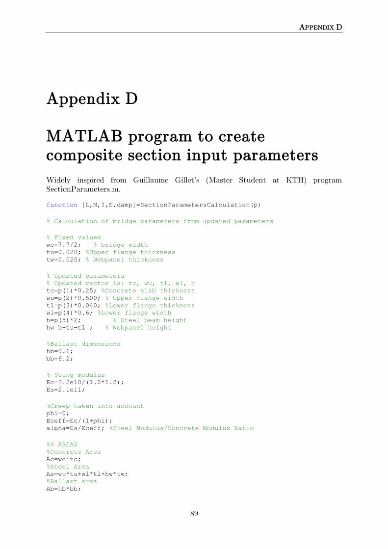
APPENDIX D
89
Appendix D MATLAB program to create composite section input parameters
Widely inspired from Guillaume Gillet’s (Master Student at KTH) program SectionParameters.m.
function [L,M,I,E,damp]=SectionParametersCalculation(p)
% Calculation of bridge parameters from updated parameters
% Fixed values wc=7.7/2; % bridge width tu=0.020; %Upper flange thickness tw=0.020; % Webpanel thickness
% Updated parameters % Updated vector is: tc, wu, tl, wl, h tc=p(1)*0.25; %Concrete slab thickness wu=p(2)*0.500; % Upper flange width tl=p(3)*0.040; %Lower flange thickness wl=p(4)*0.6; %Lower flange width h=p(5)*2; % Steel beam height hw=h-tu-tl ; % Webpanel height
%Ballast dimensions hb=0.6; bb=6.2;
% Young modulus Ec=3.2e10/(1.2*1.2); Es=2.1e11;
%Creep taken into account phi=0; Eceff=Ec/(1+phi); alpha=Es/Eceff; %Steel Modulus/Concrete Modulus Ratio
%% AREAS %Concrete Area Ac=wc*tc; %Steel Area As=wu*tu+wl*tl+hw*tw; %Ballast area Ab=hb*bb;

APPENDIX D
90
%% DENSITY %Density of concrete. Standard value= 2400 kg/m^3 mc=2400; %Density of steel. Density of steel varies between 7750 and 8050 kg/m3. % %density of mild steel: 7850; ms=7850; %Density of ballast. 2000 kg/m^3 mb=2000;
%Mass of the cross section of the bridge in kg/m Mass=mc*2*Ac+ms*2*As+mb*Ab;
%% STIFFNESS %Concrete slab Gravity Center from the bottom yc=tl+hw+tu+tc/2; %Steel Beam Gravity Center from the bottom ys=(tl/2*wl*tl+(tl+hw/2)*hw*tw+(tl+hw+tu/2)*wu*tu)/As; %Center of Gravity of the composite section from the bottom ycomp=(As*ys+yc*Ac/alpha)/Acomp; ac=yc-ycomp; as=ycomp-ys;
%Moment of Inertia of the concrete slab Ic=wc*tc^3/12; %Moment of Inertia of the steel beam Is=wl*tl^3/12+wu*tu^3/12+tw*hw^3/12+wl*tl*(ys-tl/2)^2+tw*hw*(ys-
(tl+hw/2))^2+wu*tu*(ys-(tl+hw+tu/2))^2; %1 steel beams
%Moment of inertia of the composite section Icomp=Is+As*as^2+Ic/alpha+Ac*ac^2/alpha; I=Icomp*2; %To have whole bridge, 2 parts
%% OTHER PARAMETERS L=42; E=2.1e11; material='composite'; M=Mass/1000; %[ton/m]
% Damping if (L<20) if strcmp(material,'steel') || strcmp(material,'composite') damp=(0.5+0.125*(20-L))/100; elseif strcmp(material,'prestressed_concrete') damp=(1.0+0.07*(20-L))/100; elseif strcmp(material,'filler_beam') ||
strcmp(material,'reinforced_concrete') damp=(1.5+0.07*(20-L))/100; end elseif (L>=20) if (strcmp(material,'steel') || strcmp(material,'composite')) damp=0.5/100; elseif strcmp(material,'prestressed_concrete') damp=1.0/100; elseif strcmp(material,'filler_beam') ||
strcmp(material,'reinforced_concrete') damp=1.5/100; end end

APPENDIX E
91
Appendix E MATLAB program to create open section input parameters of a ballasted ordinary concrete bridge.
function [L,M,I,E,damp]=Usection(p)
%Parameters a=7; b=p*2.7; c=1.2;
%Ballast dimensions hb=0.6; bb=a-2*c;
Ac=a*0.5+2*c*(b-0.5); %Concrete area Ab=hb*bb; %Ballast area
%Density of concrete. Standard value= 2400 kg/m^3 mc=2400; %Density of ballast. 2000 kg/m^3 mb=2000;
%Mass of the cross section in kg/m Ma=Ac*mc+Ab*mb; %Mass of the cross section in tons/m M=Ma/1000;
%Centre of gravity y=(0.5*a*0.25+c*(b-0.5)*(0.25+b/2)*2)/Ac; % Second moment of inertia I=a*0.5^3/12+a*0.5*(y-0.25)^2+2*(c*(b-0.5)^3/12+c*(b-0.5)*(y-
(0.25+b/2))^2);
L=10; % Length of the bridge Ec=3.5e10; % Young modulus in N/m^2 E=0.6*Ec; % Cracking material='reinforced_concrete';
% Damping if (L<20) if strcmp(material,'steel') || strcmp(material,'composite') damp=(0.5+0.125*(20-L))/100;

APPENDIX E
92
elseif strcmp(material,'prestressed_concrete') damp=(1.0+0.07*(20-L))/100; elseif strcmp(material,'filler_beam') ||
strcmp(material,'reinforced_concrete') damp=(1.5+0.07*(20-L))/100; end elseif (L>=20) if (strcmp(material,'steel') || strcmp(material,'composite')) damp=0.5/100; elseif strcmp(material,'prestressed_concrete') damp=1.0/100; elseif strcmp(material,'filler_beam') ||
strcmp(material,'reinforced_concrete') damp=1.5/100; end end


TRITA-BKN. Master Thesis 301,
Structural Design and Bridges 2010
ISSN 1103-4297
ISRN KTH/BKN/EX-301-SE
www.kth.se