Optimal Dam Construction under Climate Change...

Optimal Dam Construction under Climate Change Uncertainty

and Anticipated Learning

by

Patricia Jane Cameron-Loyd

A dissertation submitted in partial satisfaction of the

requirements for the degree of

Doctor of Philosophy

in

Agricultural and Resource Economics

in the

Graduate Division

of the

University of California, Berkeley

Committee in charge:

Professor Larry Karp, Chair Professor David Sunding

Associate Professor Catherine Wolfram

Spring 2012



Copyright 2012

by


Abstract



by


Doctor of Philosophy in Agricultural and Resource Economics

University of California, Berkeley

Professor Larry Karp, Chair

Public capital-investment projects are typically evaluated using standard net-present-value

(NPV) analysis. Projects with large, up-front investments, such as dams or energy plants, often

are irreversible and have uncertain future benefits. If we expect to reduce uncertainty about

these future flows over time, introducing the option to delay the project may increase project

value and lead to different decisions. This dissertation evaluates a pending California water

storage and conveyance project that would increase the capacity of an existing dam, the value of

which depends upon the future climate state. The research uses a dynamic optimization program

with two stochastic state variables to analyze decision making. One state variable is the belief

about the future climate state, and the other is the level of green-house-gas (GHG) stocks, both of

which change in a random manner. The analysis allows for the possibility of learning more about

the true state of the future climate as time goes on. The results differ substantially from those of

the policy makers involved in the empirical project.

1

To my wonderful children, Gemma, Phil and Casey, who took care of themselves when I was too

busy to make them a good dinner or to take them on a nice day trip, and who were always there

to give me hugs, kisses and encouragement.

i

Table of Contents

1 Introduction ........................................................................................................................1

2 A Model of Dam Construction Decision Making under Climate Change and

Anticipated Learning .....................................................................................................................4

2.1 Empirical Application and Data...............................................................................6

2.1.1 Parameters and variables..............................................................................7

2.1.2 Expected prices and quantities .....................................................................8

2.1.3 Possible future climate distributions ............................................................9

2.1.4 Expected learning time ..............................................................................11

2.2 Initial Problem Solution .........................................................................................14

2.3 Variable Growth of Green House Gas Levels .......................................................17

2.3.1 Deterministic GHG growth ........................................................................18

2.3.2 Stochastic GHG growth .............................................................................23

2.4 Discussion ..............................................................................................................25

3 Sensitivity Analysis ..........................................................................................................26

3.1 Restatement of Problem and Base Case.................................................................27

3.2 Parameters to be Varied and Sensitivity Analysis .................................................28

3.2.1 Change in discount rate ..............................................................................29

3.2.2 Price increase rate change ..........................................................................31

3.2.3 Change in project capital cost ....................................................................33

3.2.4 Change in benefit lifetime ..........................................................................33

3.2.5 Deterministic GHG level growth rate ........................................................35

3.3 Stochasticity in GHG-level Growth .......................................................................36

3.4 Discussion ..............................................................................................................38

4 Cost-benefit Analysis and Decision Making ..................................................................38

4.1 Cost-benefit Analysis .............................................................................................41

4.1.1 Brief history ...............................................................................................42

4.1.2 Steps to analysis .........................................................................................42

4.1.3 Problem areas using CBA ..........................................................................47

4.2 Environmental Impact Analysis .............................................................................52

4.3 Discussion ..............................................................................................................53

References .....................................................................................................................................55

ii

Acknowledgements

I first want to thank my advisor, Larry Karp. Professor Karp introduced me to an area of study

that I knew little about, and guided me carefully throughout my research. Under his tutelage I

have learned more than I could have imagined.

The faculty and staff at the University of California, Berkeley, Agricultural and Resource

Economics Department have been extremely supportive. David Sunding and Jeffrey Perloff

taught me how to teach. David Sunding and David Zilberman have consistently given me insight

into water economics in California and beyond. Brian Wright and Ethan Ligon supported me

through some tough times. Peter Berke, Sofia Villa-Boas, Catherine Wolfram, Gail Vawter and

Diana Lazo were helpful in more ways than I can write.

My classmates in the program were generous with their time and their insights, and I am amazed

that I can be counted among such a talented group. My buddies, Thomas Sproul and Sarah

Dobson, inspired me to keep going when times got tough.

Thanks also to the Giannini Foundation for financially supporting my research.

iii

1 Introduction

This research uses a speci�c Northern California dam expansion project to examinehow the anticipation of future information about climate change should be used whenevaluating large infrastructure projects. The Los Vaqueros Dam Expansion Projectwould increase the storage and conveyance capacity of an existing dam. The Bureauof Reclamation evaluated this project using a standard cost-bene�t analysis, in whichthey compare the net present value (NPV) of the future net bene�t streams with thecurrent value of the investment. (Bureau of Reclamation (BOR), 2006). The valueof the future bene�t stream depends (among other things) on the future distributionof precipitation in California. The BOR analysis assumes that historical distributionof precipitation will continue into the future.

There is extensive evidence that human-in�uenced climate change is occurring.The 2007 Fourth International Panel on Climate Change Assessment (IPCC, 2007, pg2) �nds that �Warming of the climate system is unequivocal, as is now evident fromobservations of increases in global average air and ocean temperatures, widespreadmelting of snow and ice, and rising global average sea level.� The magnitude offuture climate change is thought to be primarily dependent upon the path of annualemissions, and resultant atmospheric stock, of greenhouse gases (GHGs). The IPCCAssessment cites multiple models for the future paths of GHG emissions and stocks.The e¤ect of climate change on the precipitation distributions in California, and

hence the value of dam projects, is uncertain in terms of both timing and direction,even at known GHG levels. Di¤erent prominent models predict either dryer orwetter futures for California with increasing GHGs. In this research, I use twowidely accepted general circulation models (GCMs) to predict future precipitationdistributions. Mymaintained hypothesis is that the future climate is either becomingincreasingly wet or increasingly dry, and can be accurately predicted by one of thesetwo GCMs. I model future climate as a distribution of precipitation. There aremany other aspects of climate that could be considered in this kind of research, suchas timing of precipitation and the e¤ect of rising temperature on precipitation inthe form of snow and on annual snowpack levels, but I choose annual precipitationdistribution in order to calibrate exactly with the BOR analysis. In this way I canisolate the e¤ects of climate change and anticipated learning on decision making.The planner does not know which of these two possible precipitation futures is

true, but has a belief about it that I model as the planner�s subjective probabilitythat the true future climate is wetter. As the planner observes precipitation realiza-tions each period, he updates his belief about the true climate state using Bayesianlearning. Because the planner anticipates the ability to learn about the true nature

1

of the future climate, he can anticipate learning more about the true value of thedam.Dam projects are typically evaluated using current information to compare the

net present bene�t of constructing the dam now or of never constructing it. Thereal choice, however, is whether we construct the dam now or wait until the nextperiod, at which time we will again be faced with the choice of construction or furtherdelay. The ability to begin construction in the future, if we delay construction today,is worth something. The value of this possibility is known as the �option value�.Studies that fail to take into account this option value understate the bene�t ofdelaying construction and are therefore biased in favor of early construction. Theoption value arises because we anticipate obtaining better information in the futureabout the value of the dam.I develop a dynamic programming model of decision making, where the decision

is either to build this year or wait one year and decide again to either build or delay.The model depends on two stochastic state variables. One is the subjective belief thatthe true climate is wet. Because the precipitation (the learning signal about the trueclimate scenario) is random, this state variable is updated in a stochastic manner.The second state variable is the GHG stock level, which grows stochastically due toexogenous variability.I �nd the optimal decision given the two state variables. That is, given that we

know the current GHG level and we have a subjective belief about the true climatefuture, I determine whether we should decide to build today or not. The BORanalysis determines that the optimal decision is to build the dam. My researchconcludes that given certain parameters there is value to delaying the project unlessour belief that the future climate is the wetter one is low. Unless the policy makershave a high level of con�dence in a dryer future, they should delay building untilthey learn more about the true climate, contrary to the BOR recommendation.The World Commission on Dams (WCD) (2000) reports that the decision-making

framework on dams has traditionally been a simple cost-bene�t analysis and excludesconsideration of uncertainty with regard to future bene�ts of the dam. A dam, oncebuilt, is an irreversible investment, as it cannot be repurposed. Arrow and Fisher(1974) show that when we make an irreversible decision to develop an environmentand the bene�t is uncertain, assuming risk-neutrality, simply replacing known valueswith expectations does not capture the loss of the bene�ts in perpetuity of thea¤ected environment. Hence, the bene�ts of such an investment are overstated. Inorder to preserve these potential bene�ts, less development should occur than impliedthrough traditional cost-bene�t analysis. They combine the notion of irreversibilitywith the assumption that a realization in one period will a¤ect the expectations

2

in the next. Their model allows for the reduction of uncertainty in the secondperiod, allowing for a revision of decision-making (compressing all future periodsinto the single second period.) Irreversibility under these circumstances acts uponinvestment decisions in a manner similar to risk aversion. The key to their modelis that development is irreversible, while preservation (or the potential for futuredevelopment) is not. Their quasi-option value measures the value of informationthat is gained by learning during delay and the ability to react to that information.Dixit and Pindyck (1994) develop the concept of real option theory and use

dynamic optimization over multiple periods to improve decision making under irre-versibility, uncertainty and learning. There is an extensive literature in economicson real options in a general setting. A smaller literature (Kolstad (1996), Ulph andUlph (1997), Gollier et.al. (2000) and Karp and Zhang (2006)) studies the e¤ectof anticipated learning in the context of climate change. Several of these papers�nd that the anticipation of future learning about climate change tends to decreasecurrent e¤orts to reduce carbon emissions.When uncertainty and learning are involved in decision-making, the expected

speed of learning can a¤ect the analysis. Kelly and Kolstad (1999) apply Bayesianlearning to estimate the amount of time required to resolve uncertainties about cli-mate change e¤ects. They �nd that learning can take far longer than might beexpected intuitively, arriving too late to a¤ect decisions. Their analysis involvesactive learning, where the decision makers may in�uence the change that is learnedabout. Their theory also applies in cases of passive (exogenous) learning, as in thispaper.

As part of my analysis I examine how the rate of expected learning depends onthe initial subjective belief about the future of climate change, and how that rateof learning changes as the rate of information delivery changes. When the GHGstock changes at a faster rate, the stochastic weather realizations change at a fasterrate, delivering more useful information sooner. In some cases, the anticipation ofmore rapid learning has a positive e¤ect on the option to delay. I also examinehow learning, and thus the option value, is a¤ected when GHG stock changes arestochastic.Forsyth (2000) and Conrad and Kotani (2005) evaluate decision-making in a

forest, and in the Alaska National Wildlife Refuge, respectively. In both cases,the key state variable is the random price, which a¤ects the value of the project.Michailidis and Mattas (2005) apply real option theory in valuing a dam investment.They demonstrate that adding the management �exibility to delay, later expand orabandon a dam project improves analysis of project pro�tability when compared toa traditional NPV approach. Their underlying future asset value, based on price,

3

follows a random distribution over discrete periods.My research di¤ers from these studies in that one of my state variables is the

subjective belief about how a particular system will evolve in the future. Thus, thekey learning is not simply about the realization of a random variable. Instead theplanner understands that he will learn about a dynamic process over time, in thiscase about the evolving distribution of precipitation or climate state.The practical result of this work is to demonstrate the application of better

decision-making tools than those currently employed, using information and beliefsabout climate change, leading to the possibility of better decisions concerning majorhydrological projects. The techniques employed are applicable to assessing othertypes of long-term capital projects using beliefs about climate change or other fun-damental types of change.In the next chapter I develop the model of decision-making and make recom-

mendations on whether to build a dam today or to delay, depending on the decisionmaker�s belief about the climate future. In chapter three I perform sensitivity analy-ses, varying several key parameters to determine the degree to which small changesin these parameters a¤ect those recommendations. In the �nal chapter I discuss thestrengths and weaknesses of cost-bene�t analysis methods when deciding to build amajor dam project.

2 AModel of Dam Construction Decision Makingunder Climate Change Uncertainty and Antici-pated Learning

The policy maker needs to decide whether to build a dam today or to delay for oneperiod and decide again as he learns more about the true value of the dam, which isdependent upon the distribution of precipitation. I assume that the actual weatherpattern will follow one of two possible climate scenarios: i = 1; 2; where i = 1describes an increasingly wet climate scenario, and i = 2 describes an increasinglydry scenario. The policy maker does not know which of these two scenarios isthe true future climate, but has a belief about the true climate future. The policymaker�s belief is his subjective probability that the true climate is the increasinglywet one, p.The two possible future climate states are both modeled as a weather distribution

j which describes �ve types of precipitation levels (driest, very dry, below normal,above normal and wet) such that when j = 1 a driest type precipitation occurs(under 16 annual inches) and when j = 5 a wettest type year occurs (over 23 annual

4

inches.) The likelihood of a type j precipitation year occurring in a given year yassuming that the true climate state is i = 1; 2 is designated by fijy. Thus, as yincreases, and if i = 1 (the wetter scenario) the probability of a driest weather typej = 1 occurring will decline.I want to decide whether to add storage that is expected to produce annual

bene�ts dependent on the annual precipitation type and, because of price increases,is dependent on the year z(j; t). The bene�t will occur for T years, after which therewill be no bene�t. The bene�ts are in real dollars and are expected to change withtime as this analysis assumes annual real price increases of variable water bene�t ata constant rate of r. The decision to build the dam is irreversible due to political andpractical constraints. Construction will be completed in � years from the point ofdecision, year y, and will cost k: (Construction is expected to be delayed � years fromthe decision point due to the need to acquire congressional approval and funding,and for project design.) The capital investment k is incurred at the beginning of the"base" year, y+ � , and the stream of annual bene�ts begins to be accrued at the endof that year. The future bene�ts are discounted using an annual discount factor of�. All costs and �xed bene�ts are calculated using real price levels correspondingto the earliest possible decision year, y = 1, while prices associated with variablebene�ts increase annually at a rate r: The expected value of the project at base yeary + � if decided upon in year y when the true climate future is i is:

wiy =

T+y+��1Xt=y+�

�t��JXj=1

fijtz(j; t)

!� �y�1k: (1)

The subjective probability that the wetter climate future is the true e¤ect ofclimate change (i = 1) is p. De�ne the expected present value of the future bene�tsof the additional storage given the current beliefs about climate change as:

v(p; y) = pw1y + (1� p)w2y: (2)

If our only choice is to decide at the earliest possible decision point (y = 1), theproblem is a simple NPV calculation (where the superscript N stands for the "naive"solution):

JN(p; 1) = maxfv(p; 1); 0g (3)

We have the option to wait until some period in the future to build the dam. Astime goes on, we observe j; the precipitation that occurs at each annual observation.Using Bayes�model of learning we update our belief about the true climate state.

5

For example, if we observe a sequence of very wet years, our belief that the trueclimate is wet, p, will increase over time. Thus, the realization of j a¤ects how thebelief about the true climate is updated.The choice today is to either decide to build the dam or to wait one period and

decide again. To determine the optimal action, where j is observed in year y, Icalculate the expected value of the project by solving the dynamic programmingequation

J(p; y) = maxEp�jpfv(p; y); J(p0; y0)g (4)

subject to p�(j; p; y) =pf1jy

pf1jy + (1� p)f2jy(5)

subject to y0 = y + 1: (6)

The subjective probability that i = 1 is represented by p, and p0 denotes the valueof p in the next period, such that p0 = p0(j; p; y) as shown in Equation 5, and j, thetype of precipitation year, is an exogenous variable that will occur with probabilityfijy. Thus, the subjective probability distribution of p0 is

Pr

�p�=

pf1jypf1jy + (1� p)f2jy

�= Fpjy (7)

where Fpjy = pf1jy + (1� p)f2jy (8)

for j 2 f1; 2; :::;_j):

2.1 Empirical Application and Data

The empirical evaluation is based on the proposed addition of storage and deliverycapacity to the Los Vaqueros reservoir system in Northern California (BOR, 2006)operated by the Contra Costa Water District (CCWD). It is an o¤stream reservoir,with an intake and pumping station on the Delta. Currently the reservoir�s primarypurpose is to store water when Delta water quality is good, return water to the Deltawhen quality is bad, and to provide storage for emergencies, including drought ormajor �re.The primary purpose of the proposed new storage and conveyance system is to

transfer water from the wetter, lower-demand north to the low-volume, high-demandsouth. The value of the project is in two parts: �xed bene�ts (b) and variable

6

bene�ts (�(j)(1+ r)y � q(j)), from which annual �xed costs (c) are deducted. Thus,

z(j; y) = �(j)(1 + r)y � q(j) + b� ��:5c: (9)

2.1.1 Parameters and variables

Table 1 summarizes all of the key variables and parameters, except for prices andquantities, which are covered in the next section, and, where applicable, show thevalues used in the Bureau of Reclamation (BOR, 2006) analysis. Because my analysisonly considers the e¤ects of climate change and anticipated learning on decisionmaking, I calibrate my model to the BOR analysis, and use all of their parametervalues.

Label De�nition Valuei Possible future climate distributions. 1=wet, 2=dryj Precipitation year types from driest to wettest. 1 to 5y Index of years. 1 = 2006fijy Prob. of weather type j occurring in y if true climate is i:T Years for which the project has a positive annual bene�t. 100z(j; y) Expected annual bene�t in year y with weather-type j:� Annual discount rate applied to annual bene�ts 1=1:05125

at year�s end and to costs mid-year.� Years between dam building decision and completion. 10k Present value of one-time project capital cost at y + � : $596; 889; 000wiy Exp. NPV of project decided in year y if climate is i.p Subjective probability that i = 1:v(p; y) Expected present value of project given climate belief.q(j) Additional acre feet used in weather type year j: See Table 2�(j) Acre foot water price dependent on weather j in year y. See Table 2b Fixed annual bene�ts from increased water and �shery $12; 240:000

quality, and emergency water supplies from project.c Fixed annual operating costs. $3; 546; 100r Annual expected price increase for variable bene�ts 0.1%

Table 1: Variables list with values taken directly from Bureau of Reclamation analy-sis.

All costs and bene�ts are in real 2006 dollars; variable bene�t prices increase atan annual rate of r. In order to calibrate to the BOR analysis, nominal price and

7

cost changes due to in�ation are assumed to a¤ect all other categories equally, andare excluded from the analysis.

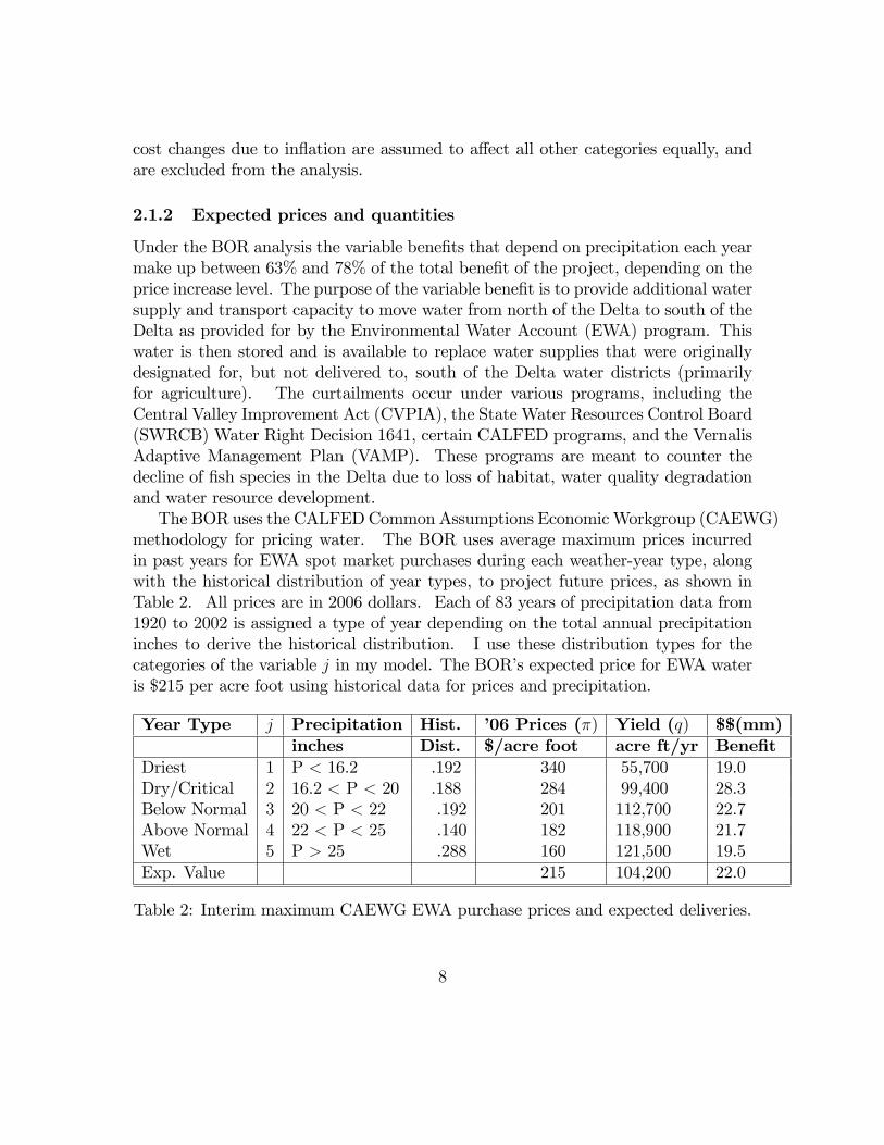
2.1.2 Expected prices and quantities

Under the BOR analysis the variable bene�ts that depend on precipitation each yearmake up between 63% and 78% of the total bene�t of the project, depending on theprice increase level. The purpose of the variable bene�t is to provide additional watersupply and transport capacity to move water from north of the Delta to south of theDelta as provided for by the Environmental Water Account (EWA) program. Thiswater is then stored and is available to replace water supplies that were originallydesignated for, but not delivered to, south of the Delta water districts (primarilyfor agriculture). The curtailments occur under various programs, including theCentral Valley Improvement Act (CVPIA), the State Water Resources Control Board(SWRCB) Water Right Decision 1641, certain CALFED programs, and the VernalisAdaptive Management Plan (VAMP). These programs are meant to counter thedecline of �sh species in the Delta due to loss of habitat, water quality degradationand water resource development.The BOR uses the CALFEDCommon Assumptions EconomicWorkgroup (CAEWG)

methodology for pricing water. The BOR uses average maximum prices incurredin past years for EWA spot market purchases during each weather-year type, alongwith the historical distribution of year types, to project future prices, as shown inTable 2. All prices are in 2006 dollars. Each of 83 years of precipitation data from1920 to 2002 is assigned a type of year depending on the total annual precipitationinches to derive the historical distribution. I use these distribution types for thecategories of the variable j in my model. The BOR�s expected price for EWA wateris $215 per acre foot using historical data for prices and precipitation.

Year Type j Precipitation Hist. �06 Prices (�) Yield (q) $$(mm)inches Dist. $/acre foot acre ft/yr Bene�t

Driest 1 P < 16.2 .192 340 55,700 19.0Dry/Critical 2 16.2 < P < 20 .188 284 99,400 28.3Below Normal 3 20 < P < 22 .192 201 112,700 22.7Above Normal 4 22 < P < 25 .140 182 118,900 21.7Wet 5 P > 25 .288 160 121,500 19.5Exp. Value 215 104,200 22.0

Table 2: Interim maximum CAEWG EWA purchase prices and expected deliveries.

8

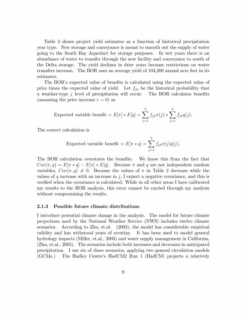
Table 2 shows project yield estimates as a function of historical precipitationyear type. New storage and conveyance is meant to smooth out the supply of watergoing to the South Bay Aqueduct for storage purposes. In wet years there is anabundance of water to transfer through the new facility and conveyance to south ofthe Delta storage. The yield declines in drier years because restrictions on watertransfers increase. The BOR uses an average yield of 104,200 annual acre feet in itsestimates.The BOR�s expected value of bene�ts is calculated using the expected value of

price times the expected value of yield. Let fjh be the historical probability thata weather-type j level of precipitation will occur. The BOR calculates bene�ts(assuming the price increase r = 0) as

Expected variable bene�t = E[�] � E[q] =5Xj=1

fjh�(j) �5Xj=1

fjhq(j):

The correct calculation is

Expected variable bene�t = E[� � q] =5Xj=1

fjh�(j)q(j):

The BOR calculation overstates the bene�ts. We know this from the fact thatCov(�; q) = E[� � q] � E[�] � E[q]. Because � and q are not independent randomvariables, Cov(�; q) 6= 0. Because the values of � in Table 2 decrease while thevalues of q increase with an increase in j, I expect a negative covariance, and this isveri�ed when the covariance is calculated. While in all other areas I have calibratedmy results to the BOR analysis, this error cannot be carried through my analysiswithout compromising the results.

2.1.3 Possible future climate distributions

I introduce potential climate change in the analysis. The model for future climateprojections used by the National Weather Service (NWS) includes twelve climatescenarios. According to Zhu, et.al. (2003), the model has considerable empiricalvalidity and has withstood years of scrutiny. It has been used to model generalhydrology impacts (Miller, et.al., 2003) and water supply management in California,(Zhu, et.al., 2005). The scenarios include both increases and decreases in anticipatedprecipitation. I use six of these scenarios, applying two general circulation models(GCMs.) The Hadley Centre�s HadCM2 Run 1 (HadCM) projects a relatively

9

warmer, wetter California, while the National Center for Atmospheric Research�sParallel Climate Model Run B06.06 (PCM) projects a relatively dryer and coolerscenario. Both models assume a 1% annual increase in GHG emissions and projectfor three future periods: 2010-2039, 2050-2079 and 2080-2099, as shown in Table 3 :

Model Period Temperature PrecipitationChange (Mean) PercentageDegrees Celsius Change (Mean)

HadCM 2010-�39 1.4 26HadCM 2050-�79 2.4 32HadCM 2080-�99 3.3 62PCM 2010-�39 0.4 - 2PCM 2050-�79 1.5 -12PCM 2080-�99 2.3 -26

Table 3: Projected 100-year changes in precipitation and in temperature under theHadley Climate Model and the Parallel Climate Model.

I apply these projected changes by changing the 83 historical observations ofyearly California precipitation inches by the appropriate percentage and categorizingthe results into the �ve weather-year types used by the BOR, resulting in two di¤erentfuture precipitation patterns. For example, over the historical 83 years, there were16 years for which the annual precipitation was fewer than16 inches, ranging from 9.2inches to 15.8, qualifying as a driest type year. Since 16 is 19.2% of the 83 years, thehistorical likelihood of a driest type year occurring is 19.2%. I apply the expected26% mean increase under the HadCM model that will occur in the period 2010-�39 toeach of these 16 precipitation amounts, and come up with an adjusted range of 11.6inches to 19.9 inches, of which only two observations are less than 16 inches. Twoobservations out of 83 imply that in the 2010-2039 period, the mean percentage ofyears that will be driest occur with a likelihood of 2.4%. Table 4 gives the resultingconditional probabilities that describe the likelihood that a given year�s precipitationwill be at a particular level given that the true future climate is accurately predictedby the HadCM or the PCM model. (The headings 2025, 2065 and 2090 refer to themean year of the projection, for example the header "2025" represents the period2010-�39.)

10

Climate Model Historical HadCM PCMi = 0 i = 1 i = 2

Period All 2025 2065 2090 2025 2065 2090

Driest .192 .024 .024 .012 .313 .361 .506Dry/Critical .188 .048 .012 .012 .229 .181 .181Below Normal .192 .254 .254 .012 .181 .229 .169Above Normal .140 .096 .108 .072 .108 .084 .084Wet .288 .578 .602 .892 .169 .145 .060

Table 4: Conditional precipitation distribution under possible future climate models

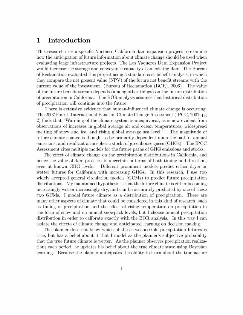
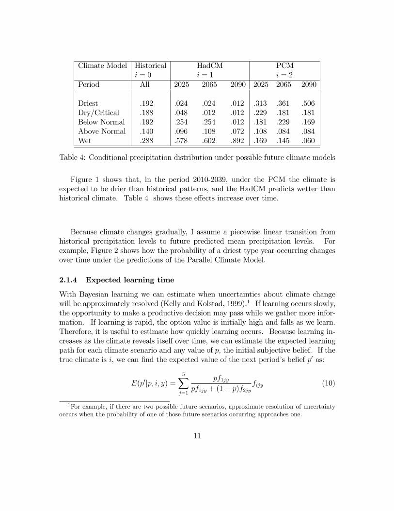
Figure 1 shows that, in the period 2010-2039, under the PCM the climate isexpected to be drier than historical patterns, and the HadCM predicts wetter thanhistorical climate. Table 4 shows these e¤ects increase over time.

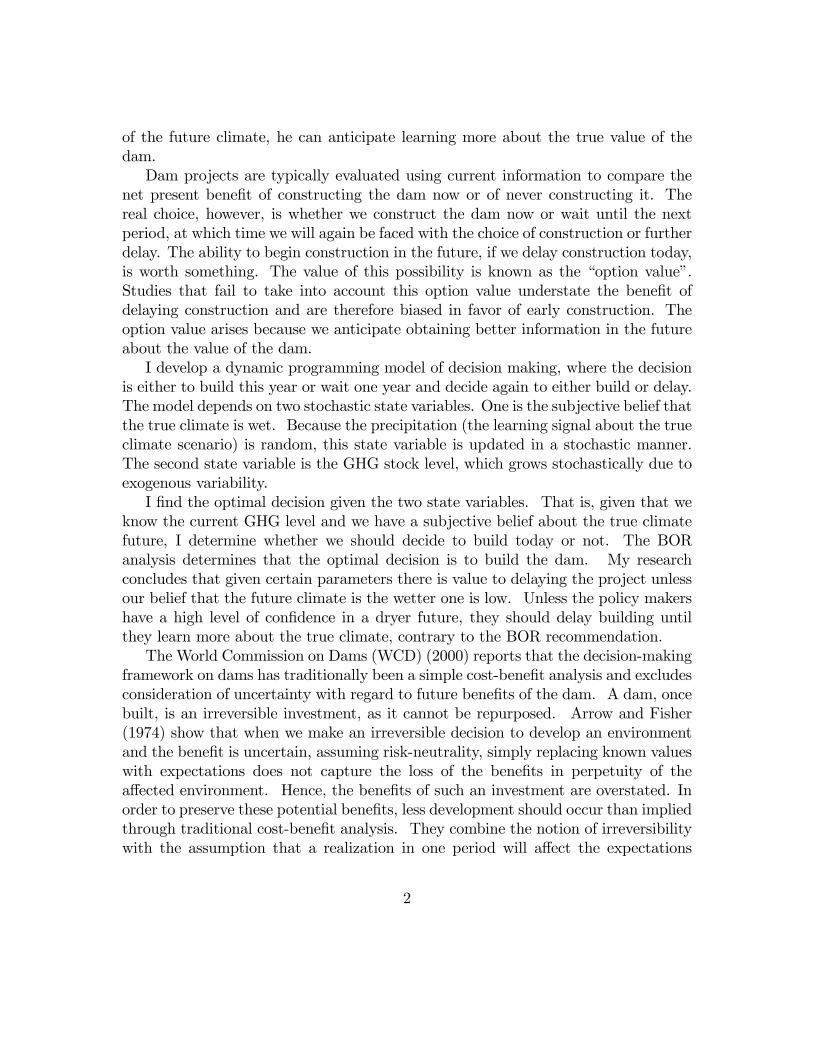
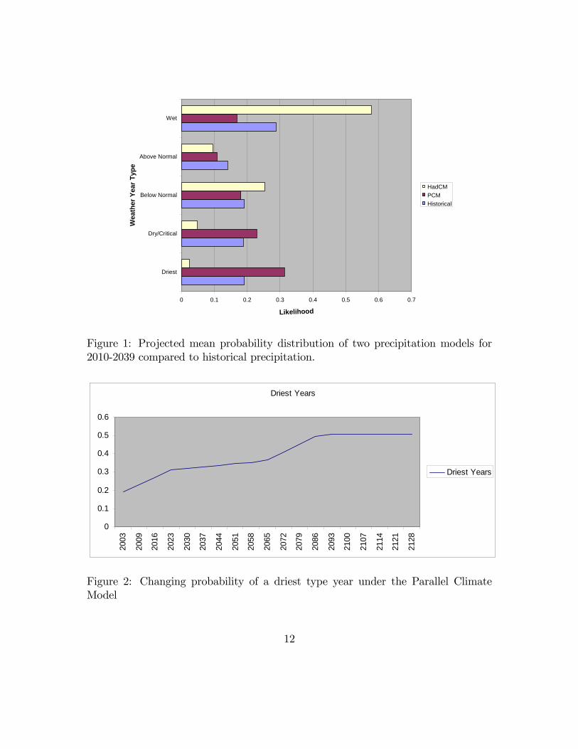
Because climate changes gradually, I assume a piecewise linear transition fromhistorical precipitation levels to future predicted mean precipitation levels. Forexample, Figure 2 shows how the probability of a driest type year occurring changesover time under the predictions of the Parallel Climate Model.

2.1.4 Expected learning time

With Bayesian learning we can estimate when uncertainties about climate changewill be approximately resolved (Kelly and Kolstad, 1999).1 If learning occurs slowly,the opportunity to make a productive decision may pass while we gather more infor-mation. If learning is rapid, the option value is initially high and falls as we learn.Therefore, it is useful to estimate how quickly learning occurs. Because learning in-creases as the climate reveals itself over time, we can estimate the expected learningpath for each climate scenario and any value of p, the initial subjective belief. If thetrue climate is i, we can �nd the expected value of the next period�s belief p0 as:

E(p0jp; i; y) =5Xj=1


fijy (10)

1For example, if there are two possible future scenarios, approximate resolution of uncertaintyoccurs when the probability of one of those future scenarios occurring approaches one.

11

0 0.1 0.2 0.3 0.4 0.5 0.6 0.7

Driest

Dry/Critical

Below Normal

Above Normal

Wet

Wea

ther

Yea

r Typ

e

Likelihood

HadCMPCMHistorical

Figure 1: Projected mean probability distribution of two precipitation models for2010-2039 compared to historical precipitation.

Driest Years

0

0.1

0.2

0.3

0.4

0.5

0.6

2003

2009

2016

2023

2030

2037

2044

2051

2058

2065

2072

2079

2086

2093

2100

2107

2114

2121

2128

Driest Years

Figure 2: Changing probability of a driest type year under the Parallel ClimateModel

12

0 10 20 30 400.2

0.3

0.4

0.5

0.6

0.7

0.8

0.9

1

Years (y=1=2006)

Subj.

Pro

b. T

hat H

adCM

Tru

e" M

odel

HadCM True Climate

0 10 20 30 400

0.1

0.2

0.3

0.4

0.5

0.6

0.7

0.8

Years (y=1=2006)

Subj.

Pro

b. T

hat H

adCM

is "T

rue"

Mod

el

PCM True Climate

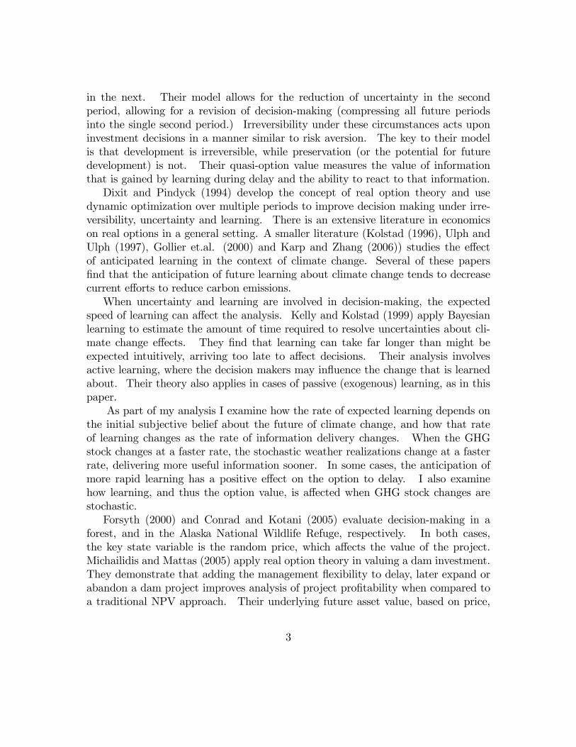
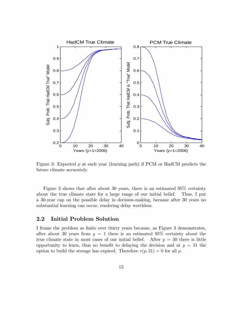
Figure 3: Expected p at each year (learning path) if PCM or HadCM predicts thefuture climate accurately.

Figure 3 shows that after about 30 years, there is an estimated 95% certaintyabout the true climate state for a large range of our initial belief. Thus, I puta 30-year cap on the possible delay in decision-making, because after 30 years nosubstantial learning can occur, rendering delay worthless.

2.2 Initial Problem Solution

I frame the problem as �nite over thirty years because, as Figure 3 demonstrates,after about 30 years from y = 1 there is an estimated 95% certainty about thetrue climate state in most cases of our initial belief. After y = 30 there is littleopportunity to learn, thus no bene�t to delaying the decision and at y = 31 theoption to build the storage has expired. Therefore v(p; 31) = 0 for all p.

13

If the delay were limited to only one or two years, a closed-form solution is easilyfound. However, expanding the problem over a full thirty years of possible delaybecomes intractable because the number of possible paths that p can take is 530.Therefore, I use interpolation estimation to approximate a solution to the problem.The general solution method is derived from Miranda and Fackler (2002.)I use numerical interpolation methods to estimate the bi-variate function2:

J(p; y) = maxfv(p; y); Ep0jp�J(p0; y0)g (11)

subject to p�(j; p; y) =pf1jy

pf1jy + (1� p)f2jy(12)

y0 = y + 1: (13)

where

Pr

�p�=


�= Fpjy (14)

To estimate the function v(p; y), I �rst de�ne a set of interpolation nodes:p 2 (0; 1) over n1 = 30 unevenly spaced breakpoints. For derivation of break-

points, see Miranda and Fackler 2002, page 129.

y = 1; 2; :::;_

Y ; where for the initial problem�Y = 30 = n2:

Given these two state variables, there are a total of N = �2i=1ni = 900 nodes.Next, I de�ne an N = 900-degree function basis using cubic splines as basis

functions. I develop an N by N interpolation matrix using the function basis andnodes and derive �(p; y), a tensor product of the univariate interpolation matrices forthe set of N known linearly independent basis functions. For a detailed descriptionof the derivation of �(p; y), see Miranda and Fackler (2002), especially page 131.I �rst evaluate v(p; y) at the N selected interpolation nodes, and then derive a

curve-�tting estimation function by approximating the solution to the value functionv(p; y):

^v(p; y) = C�(p; y) (15)

where C = basis coe¢ cients which are to be determined. To �nd basis coe¢ cients,C, I solve the linear equation:

C�(p; y) = V (p; y):

C = V=�;

2See Equation 8 for de�nition of Fpjy:

14

where V (p; y) is a solution matrix of explicit function values over the 900 interpolationnodes. Once I solve for C, I can estimate the value function for any p; y usingEquation 15.The �nite Bellman Equation 11 is solved using backward induction. The solution

to v(p; 31) = 0 for all nodes; because the option to delay building the dam expires inyear 30 when no more learning can occur. I estimate the solution for v(p; 30):

^v(p; 30) = C�(p; 30): (16)

I now estimate the expected solution to the dynamic programming equation as-suming the decision is made in year 29:

J(p; 29) = max[v(p; 29); Ep0jpf^v(p0; 30) = C�(p0; 30)g] (17)

Once I have an estimated solution for Equation 17, I solve Bellman Equation forthe prior year:

J(p; 28) = max[v(p; 28); Ep0jpJ(p0; 29)g]:

I continue the backward induction process until I estimate J(p; 1); which maxi-mizes the problem for all nodes when year y = 1. The option value is the estimatedvalue of the ability to delay

OptionV alue = J(p; 1)� v(p; 1):

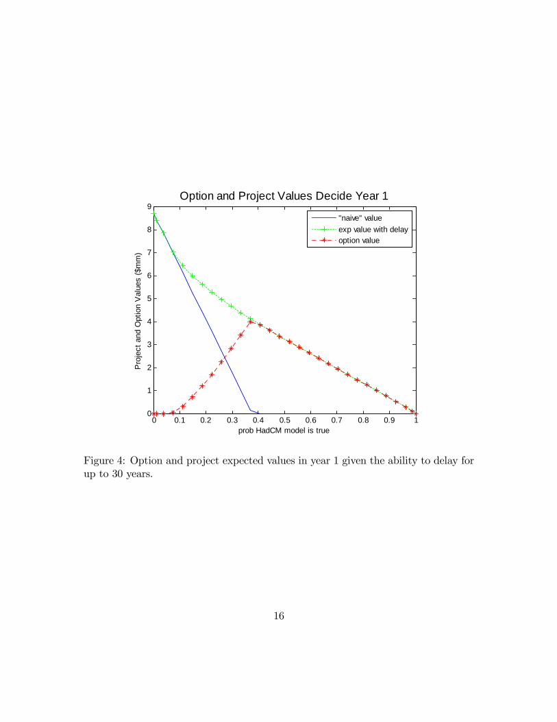
Figure 4 shows the solution for decision-making in Year 1.We are better o¤ proceeding with the project without delay only if we believe

with a probability of under .08 that the true climate will follow the wet climate model�thus it is valuable to wait to learn more about the climate before proceeding overmost of the belief space.

2.3 Variable Growth of Greenhouse Gas Levels

The HadCM and the PCM both assume that greenhouse gas stocks are increasingat a steady 1.3% rate every year, as have I so far in this paper. The solution to thisproblem might di¤er if GHG growth is at a di¤erent rate or is random. To evaluatethese cases, I assume that there is a direct relationship between the GHG level andthe precipitation distribution under a wet or dry climate type.Let

15

0 0.1 0.2 0.3 0.4 0.5 0.6 0.7 0.8 0.9 10

1

2

3

4

5

6

7

8

9

prob HadCM model is true

Pro

ject

and

Opt

ion

Val

ues

($m

m)

Option and Project Values Decide Year 1

"naive" valueexp value with delayoption value

Figure 4: Option and project expected values in year 1 given the ability to delay forup to 30 years.

16

g be the annual percentage growth rate of GHG, andG be the GHG level, such thatGjy; g is the GHG level in year y given a GHG growth rate of g.As a normalization, I set G = 1 as of the beginning of year 2003 in order to

calibrate with the HadCM and PCM scenarios. I previously assigned the valuey = 1 to the �rst possible decision year of 2006. Thus, Gjy=1;g=:013 = 1:0133: Thedistribution of weather types under either the wet (HadCM) or dry (PCM) climatemodels for the year 2006 can be associated with a GHG level of 1.0395. Similarly, thedistribution of weather types for the year 2009 can be associated with a Gjy=4;g=:013 =1.0136, or G = 1:0806. Assuming g = :013, simplify the notation to Gy = 1:013y+2:Recall that fijy is the conditional probability of observing signal j (precipitation

type) in the year y given the true climate state is i. If the climate pattern dependson the GHG level regardless of the year in which it occurs, we can replace theformer relationship between climate distributions and time with climate distributionsconditional upon GHG levels �that is map fijy to fijG.

The inverse of the relationship G = 1:013y+2 is

y + 2 = log1:013G

y = log1:013G� 2

y =lnG

ln 1:013� 2 (18)

With this transformation I map fijy to fijG. Restating the weather distributionfrom fijy to fijG allows for analysis when deterministic GHG growth is at a rateother than 1.3%.I �rst explore how the results change when the deterministic growth rate varies

from 1.3% annually. Secondly I consider what happens when GHG levels grow sto-chastically. In that case we might expect more uncertainty to increase the optionvalue of waiting.

2.3.1 Deterministic GHG growth

Suppose that GHG levels are increasing at a steady and predictable rate, g perperiod (year). There is an option to make a decision in year 2006 when y = 1, andGjy; g = (1 + g)y+2 = (1 + g)3: I restate the problem as a function of the GHGlevel G by replacing the time variable y with the transformation y = lnG

ln 1:013� 2:

As before, the capital investment k is incurred at the beginning of the base year, �years after the decision when G�+y = (1 + g)�+y+2: The bene�ts begin at the endof the base year and accrue over time at the end of each year. The future bene�ts

17

are discounted using an annual discount factor of �. All costs and bene�ts arecalculated using real price levels corresponding to the earliest possible decision year,when Gy=1;g = (1 + g)3, except for the variable bene�ts which are increased at anannual rate of r. The expected value of the project at base GHG level Gjy + � ; g ifdecided upon when GHG levels = Gjy; g and the true climate future is i is:

wiG =

0@T+ lnGln 1:013

+��3Xt= lnG

ln 1:013�2+�

JXj=1

�t��fijG(t)z(j; t)

1A� � lnGln 1:013

�3k (19)

where G(t) = (1 + g)t+2 (20)

Let p be the subjective probability that i = 1 (the wetter HadCM re�ects thetrue climate state). De�ne the expected present value of the future bene�ts of theadditional storage given the current belief about climate change, GHG level andexpected growth in GHG level g, as:

v(p;G) = pw1G + (1� p)w2G: (21)

Restate the value function as a function of our belief in the probability of a wetclimate state being true, p, and of greenhouse gas levels G, where GHG levels growat a rate g.

J(p;G) = max[Ep�jpfv(p;G); J(p0; G0)g] (22)

subject to p0(p; j; G) =pf1jG

pf1jG + (1� p)f2jG

subject to G0 = G � (1 + g)where

Pr

�p�=

pf1jGpf1jG + (1� p)f2jG

�= FpjG:

Expected learning time with variable growth rate. When we assumed thatg=.013, we found that after approximately 30 years there would be a high certaintyabout the true climate state, such that the option value after 30 years approaches 0.If GHG levels grow at a faster rate learning should occur more quickly. For example,if the true climate is dry, and GHG levels grow faster, we are likely to observe moredry years sooner �thus we will update our belief more quickly to re�ect the truestate of nature. To illustrate, I restate Equation 10 to be a function of the GHG level

18

0 5 10 15 20 25 30 35 40 45 500.2

0.3

0.4

0.5

0.6

0.7

0.8

0.9

1

Years (y=1=2006)

Sub

j. P

rob.

Tha

t Had

CM

is "

True

" M

odel

Trajectory of Expected "p"|HadCM True Climate

ghg growth rate .017ghg growth rate .006

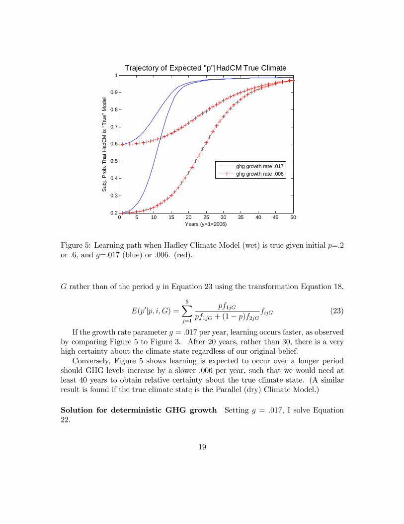
Figure 5: Learning path when Hadley Climate Model (wet) is true given initial p=.2or .6, and g=.017 (blue) or .006. (red).

G rather than of the period y in Equation 23 using the transformation Equation 18.

E(p0jp; i; G) =5Xj=1


fijG (23)

If the growth rate parameter g = .017 per year, learning occurs faster, as observedby comparing Figure 5 to Figure 3. After 20 years, rather than 30, there is a veryhigh certainty about the climate state regardless of our original belief.Conversely, Figure 5 shows learning is expected to occur over a longer period

should GHG levels increase by a slower .006 per year, such that we would need atleast 40 years to obtain relative certainty about the true climate state. (A similarresult is found if the true climate state is the Parallel (dry) Climate Model.)

Solution for deterministic GHG growth Setting g = :017, I solve Equation22.

19

0 0.1 0.2 0.3 0.4 0.5 0.6 0.7 0.8 0.9 10

1

2

3

4

5

6

7

8


Pro

ject

and

Opt

ion

Val

ues

($m

m)

Option and Project Values g=.017


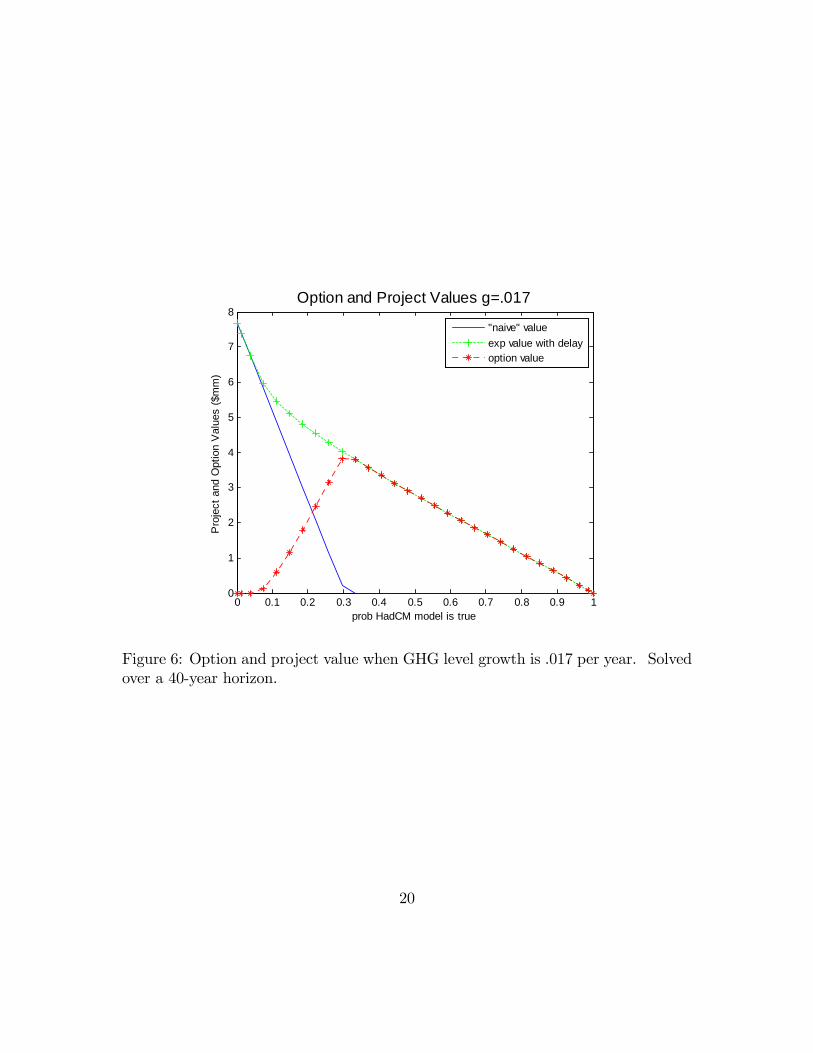
Figure 6: Option and project value when GHG level growth is .017 per year. Solvedover a 40-year horizon.

20

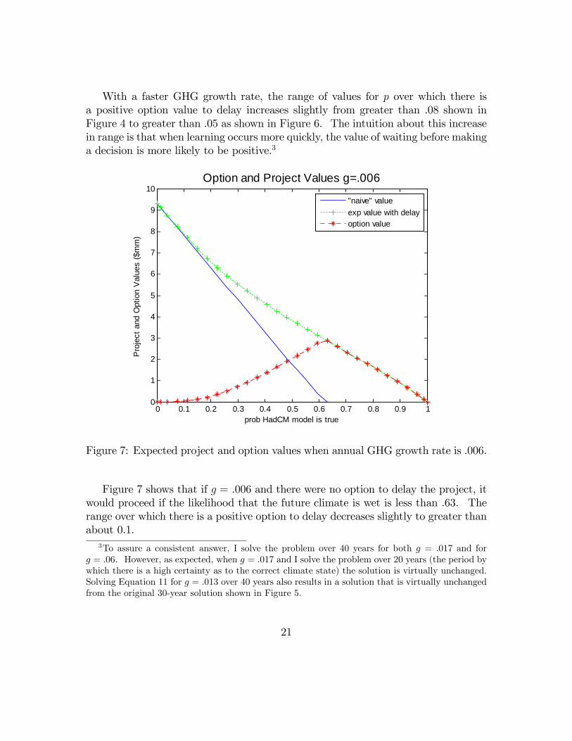
With a faster GHG growth rate, the range of values for p over which there isa positive option value to delay increases slightly from greater than .08 shown inFigure 4 to greater than .05 as shown in Figure 6. The intuition about this increasein range is that when learning occurs more quickly, the value of waiting before makinga decision is more likely to be positive.3

0 0.1 0.2 0.3 0.4 0.5 0.6 0.7 0.8 0.9 10

1

2

3

4

5

6

7

8

9

10


Pro

ject

and

Opt

ion

Val

ues

($m

m)

Option and Project Values g=.006


Figure 7: Expected project and option values when annual GHG growth rate is .006.

Figure 7 shows that if g = .006 and there were no option to delay the project, itwould proceed if the likelihood that the future climate is wet is less than .63. Therange over which there is a positive option to delay decreases slightly to greater thanabout 0.1.

3To assure a consistent answer, I solve the problem over 40 years for both g = :017 and forg = :06. However, as expected, when g = :017 and I solve the problem over 20 years (the period bywhich there is a high certainty as to the correct climate state) the solution is virtually unchanged.Solving Equation 11 for g = :013 over 40 years also results in a solution that is virtually unchangedfrom the original 30-year solution shown in Figure 5.

21

0 0.1 0.2 0.3 0.4 0.5 0.6 0.7 0.8 0.9 10

0.5

1

1.5

2

2.5

3

3.5

4


Pro

ject

and

Opt

ion

Val

ues

($m

m)

Option Value with Varied GHG Growth

option value, g=.013option value g=.006option value g=.017

Figure 8: Option values dependent on constant GHG-level growth rate.

22

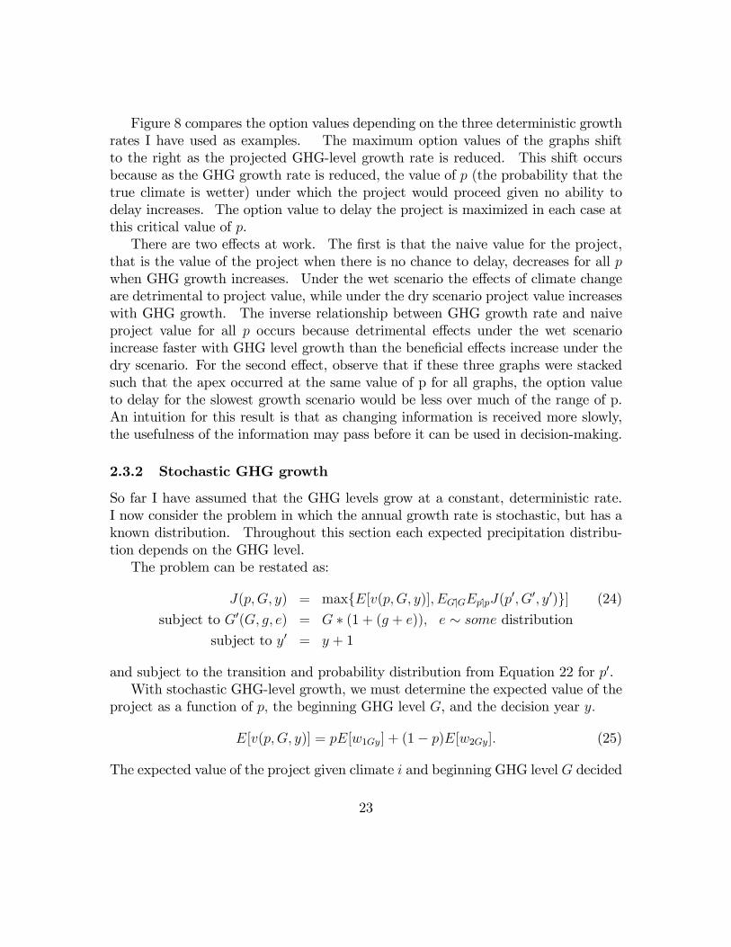
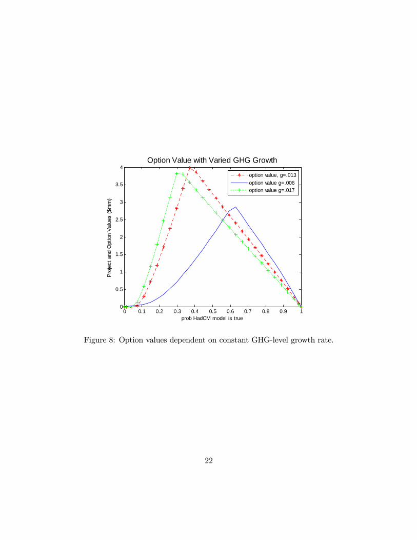
Figure 8 compares the option values depending on the three deterministic growthrates I have used as examples. The maximum option values of the graphs shiftto the right as the projected GHG-level growth rate is reduced. This shift occursbecause as the GHG growth rate is reduced, the value of p (the probability that thetrue climate is wetter) under which the project would proceed given no ability todelay increases. The option value to delay the project is maximized in each case atthis critical value of p.There are two e¤ects at work. The �rst is that the naive value for the project,

that is the value of the project when there is no chance to delay, decreases for all pwhen GHG growth increases. Under the wet scenario the e¤ects of climate changeare detrimental to project value, while under the dry scenario project value increaseswith GHG growth. The inverse relationship between GHG growth rate and naiveproject value for all p occurs because detrimental e¤ects under the wet scenarioincrease faster with GHG level growth than the bene�cial e¤ects increase under thedry scenario. For the second e¤ect, observe that if these three graphs were stackedsuch that the apex occurred at the same value of p for all graphs, the option valueto delay for the slowest growth scenario would be less over much of the range of p.An intuition for this result is that as changing information is received more slowly,the usefulness of the information may pass before it can be used in decision-making.

2.3.2 Stochastic GHG growth

So far I have assumed that the GHG levels grow at a constant, deterministic rate.I now consider the problem in which the annual growth rate is stochastic, but has aknown distribution. Throughout this section each expected precipitation distribu-tion depends on the GHG level.The problem can be restated as:

J(p;G; y) = maxfE[v(p;G; y)]; EG�jGEp�jpJ(p0; G0; y0)g] (24)

subject to G0(G; g; e) = G � (1 + (g + e)); e � some distributionsubject to y0 = y + 1

and subject to the transition and probability distribution from Equation 22 for p0.With stochastic GHG-level growth, we must determine the expected value of the

project as a function of p; the beginning GHG level G, and the decision year y:

E[v(p;G; y)] = pE[w1Gy] + (1� p)E[w2Gy]: (25)

The expected value of the project given climate i and beginning GHG level G decided

23

upon in year y can be written using a Bellman Equation

E[wiGy] = E[Vi(G; y)]� �y�1kwhere

E[Vi(G; y)] =JXj=1

fijG � z(j; y + �) + EG0jG[Vi(G0; y0)]

subject to G0(G; g; e) = G � (1 + (g + e)); e � some distributionsubject to y0 = y + 1:

Figure 9: Option values when GHG stock changes are stochastic, with normal dis-tributions and variances of .04 and .16.

Figure 9 shows the solution to Equation 24 when e follows a normal distributionwith mean = 0, and the variance in GHG growth is either .04 or .16, as comparedto the results when the variance = 0. The mean growth rate over time in all casesremains g = :013: In the case of the smaller variance, the option value is reduced overmuch of the range of p. This result may appear counterintuitive, as most modelshave found that greater stochasticity leads to higher option values. Why does theaddition of stochastic GHG growth reduce the value with delay in some cases? Theintuition for this result is that the stochasticity in the GHG level slows our learning.

24

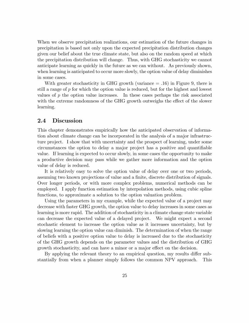
When we observe precipitation realizations, our estimation of the future changes inprecipitation is based not only upon the expected precipitation distribution changesgiven our belief about the true climate state, but also on the random speed at whichthe precipitation distribution will change. Thus, with GHG stochasticity we cannotanticipate learning as quickly in the future as we can without. As previously shown,when learning is anticipated to occur more slowly, the option value of delay diminishesin some cases.With greater stochasticity in GHG growth (variance = .16) in Figure 9, there is

still a range of p for which the option value is reduced, but for the highest and lowestvalues of p the option value increases. In these cases perhaps the risk associatedwith the extreme randomness of the GHG growth outweighs the e¤ect of the slowerlearning.

2.4 Discussion

This chapter demonstrates empirically how the anticipated observation of informa-tion about climate change can be incorporated in the analysis of a major infrastruc-ture project. I show that with uncertainty and the prospect of learning, under somecircumstances the option to delay a major project has a positive and quanti�ablevalue. If learning is expected to occur slowly, in some cases the opportunity to makea productive decision may pass while we gather more information and the optionvalue of delay is reduced.It is relatively easy to solve the option value of delay over one or two periods,

assuming two known projections of value and a �nite, discrete distribution of signals.Over longer periods, or with more complex problems, numerical methods can beemployed. I apply function estimation by interpolation methods, using cubic splinefunctions, to approximate a solution to the option valuation problem.Using the parameters in my example, while the expected value of a project may

decrease with faster GHG growth, the option value to delay increases in some cases aslearning is more rapid. The addition of stochasticity in a climate change state variablecan decrease the expected value of a delayed project. We might expect a secondstochastic element to increase the option value as it increases uncertainty, but byslowing learning the option value can diminish. The determination of when the rangeof beliefs with a positive option value to delay is increased due to the stochasticityof the GHG growth depends on the parameter values and the distribution of GHGgrowth stochasticity, and can have a minor or a major e¤ect on the decision.By applying the relevant theory to an empirical question, my results di¤er sub-

stantially from when a planner simply follows the common NPV approach. This

25

analysis suggests questions a planner should ask and, where possible, incorporate inthe analysis, for example:1) What uncertainties exist with respect to the potential value of the project?2) Under which of these scenarios does the value of the project change more

rapidly, and is that change positive or negative?3) Is there a way to quantify a possible distribution of values and probabilities

resulting from these uncertainties?4) Will there be measurable information forthcoming that will allow us to learn

and update our belief about these distributions?5) Will this information come quickly enough for the option to delay to have a

positive value?This chapter demonstrates empirically how an analysis taking into account these

questions can be done, and if enough information about parameter values is available,methods to improve decision-making with the objective of improving expected resultsof major capital projects.Future theoretical work could explore the general circumstances under which op-

tion values increase or decrease when stochasticity a¤ects the transition of more thanone state variable, particularly when the transition of one stochastic variable (learn-ing) is dependent upon the other stochastic variable. It may address the questionas to how to determine when increased uncertainty outweighs slower learning. Inaddition, more practical empirical studies could be performed to improve the method-ology of valuing projects that possess the option to delay and for which there existssome likely distributions of positive and negative outcomes that are scienti�callyjusti�ed.

3 Sensitivity Analysis

In Chapter 2, I analyze a speci�c water storage project, the Los Vaqueros DamExpansion Project, and conclude that given the anticipation of learning about thee¤ects of climate change there is a positive option value to delay the project undersome circumstances. I also �nd that the option value is reduced in some cases whengreenhouse gas (GHG) level growth stochasticity is added to the problem. I assumespeci�c parameters in reaching these conclusions, most of which are provided fromthe original Bureau of Reclamation (2006) analysis. In this chapter I vary some ofthe key parameters and analyze the e¤ect on the conclusions from Chapter 2.In conducting a project evaluation it is important to consider possible changes

to parameter values, as there are uncertainties associated with future bene�t andcost �ows, especially for long-term projects. Sensitivity analysis allows the decision

26

maker to understand the e¤ect if an uncertain parameter changes from its expectedvalue. If a small change in a parameter value leads to a large change in projectvalue, e¤orts to manage the parameter value should be implemented. If a parametervalue can vary widely resulting in potential project value change, the e¤ect of thisvariation must be considered.In this chapter I analyze changes in the discount rate, projected prices, capital

investment, project bene�t lifespan and rate of GHG-level growth. For each variableI answer the following three questions: 1) Above or below what parameter valuedoes the project have a zero (or negative) value? 2) What is the range of parametervalues for which the project would be done if there were no option to delay? 3)What is the range of parameter values for which there is a positive option to delay?I assume in each of these cases that GHG-growth is deterministic, but conclude thischapter by reviewing how varying GHG growth stochasticity a¤ects my base caseresults.

3.1 Restatement of Problem and Base Case

Recall that the problem I solve is:

J(p;G) = max[Ep�jpfv(p;G); J(p0; G0)g] (26)

subject to p0(p; j; G) =pf1jG

pf1jG + (1� p)f2jG

subject to G0(G; g; e) = G � (1 + (g + e)); e � some distribution (27)

where the probability distribution of p0 is

Pr

�p�=


�= FpjG

andv(p;G) = pw1G + (1� p)w2G (28)

27

given that

wiG =

0@T+ lnGln 1:013

+��3Xt= lnG

ln 1:013�2+�

JXj=1

�t��fijG(t)z(j; t)

1A� � lnGln 1:013

�3k (29)

where G(t) = (1 + (g + e))t+2; e � some distribution. (30)

Equation 26 is the Bellman equation that solves for the value of the project giventhe optimal decision on when to build the dam. Equation 28 is the value of theproject given a beginning GHG level, G, and a belief that the likelihood that a wetclimate future will occur is p. Equation 29 is the expected pro�t for a project givena beginning GHG level G and a known climate future i, where i = 1 represents awet climate future (the Hadley Centre Model, HadCM) and i = 2 represents a dryclimate future (the Parallel Climate Model, PCM.) The option value of delaying theproject is calculated as

OptionV alue = J(p;G)� v(p;G)

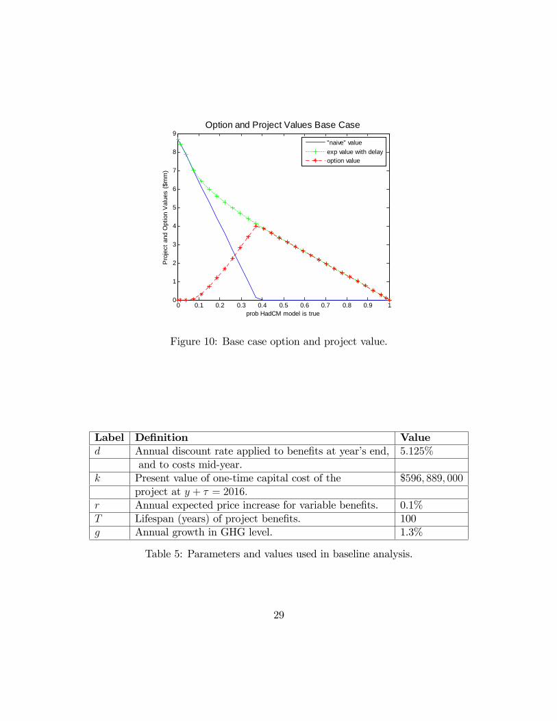
where v(p;G) is the expected value of the project when the decision is made at GHGlevel G, and there is no possibility of delay, what I call the naive project value. Forthe base case I assume G is the GHG level in the year 2006. For a full description ofthe problem and de�nitions of the parameters and values used, refer to Chapter 2.Figure 10 shows the project and option values under the base case scenario. Under

the naive solution, the project has a positive value when p < :38, and would not bepursued otherwise. With the option to delay, the project has a positive expectedvalue for all p, and a positive option value if p > :08, with a peak option value ofabout $4 million if p = :38.

3.2 Parameters to be Varied and Sensitivity Analysis

Table 5 describes the parameters that will be varied in this sensitivity analysis andtheir values under the base case. For each variable, I calculate the range over whichthe project would never be done, the range over which the project would be done ifthere were no option to delay (the naive solution) and the range over which there isa positive value to delay. These calculations vary depending on our belief that thetrue climate is wet as expressed by the probability p: I note the corner solutions atp = 1 because when we are certain the future climate is wet, the relevant projectand option values are more likely to be zero than for other values of p.

28

0 0.1 0.2 0.3 0.4 0.5 0.6 0.7 0.8 0.9 10

1

2

3

4

5

6

7

8

9


Pro

ject

and

Opt

ion

Val

ues

($m

m)

Option and Project Values Base Case


Figure 10: Base case option and project value.

Label De�nition Valued Annual discount rate applied to bene�ts at year�s end, 5:125%

and to costs mid-year.k Present value of one-time capital cost of the $596; 889; 000

project at y + � = 2016:r Annual expected price increase for variable bene�ts. 0.1%T Lifespan (years) of project bene�ts. 100g Annual growth in GHG level. 1.3%

Table 5: Parameters and values used in baseline analysis.

29

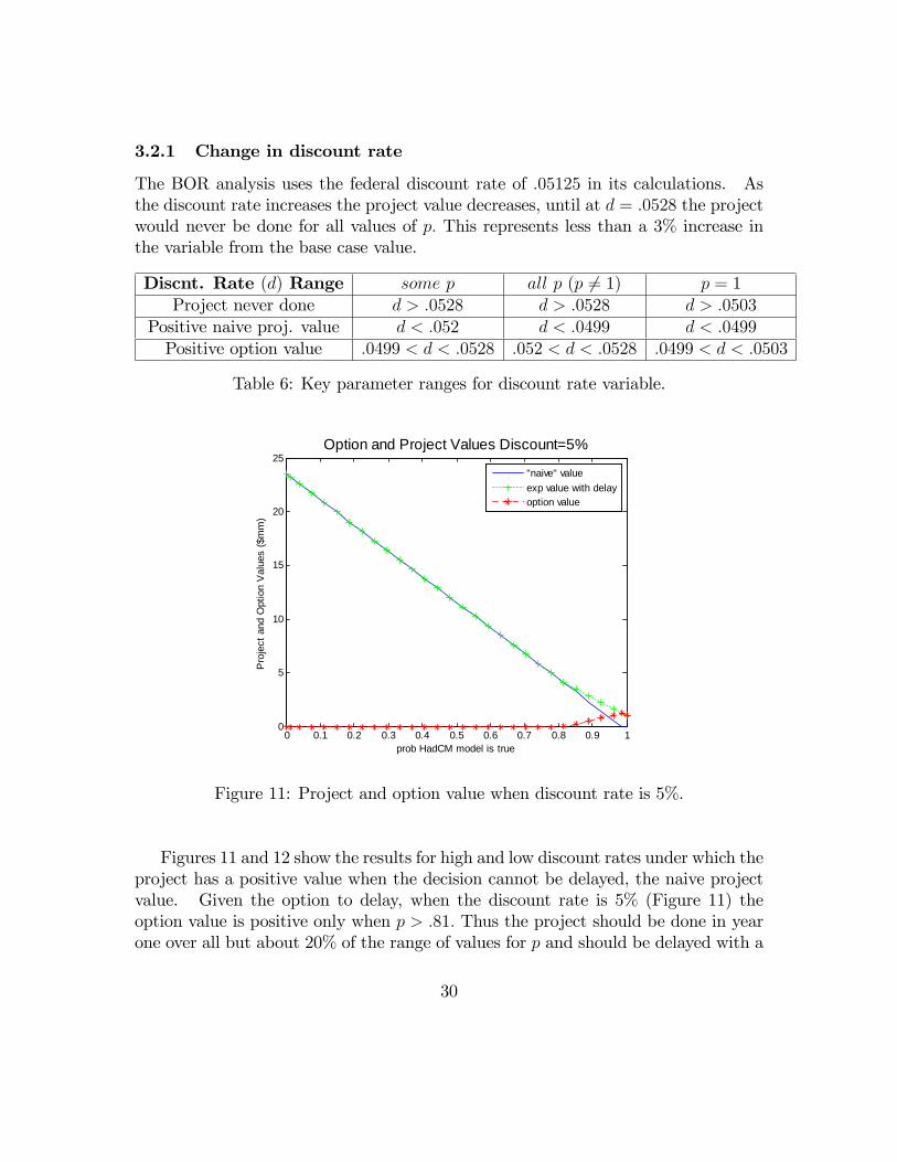
3.2.1 Change in discount rate

The BOR analysis uses the federal discount rate of :05125 in its calculations. Asthe discount rate increases the project value decreases, until at d = :0528 the projectwould never be done for all values of p: This represents less than a 3% increase inthe variable from the base case value.

Discnt. Rate (d) Range some p all p (p 6= 1) p = 1Project never done d > :0528 d > :0528 d > :0503

Positive naive proj. value d < :052 d < :0499 d < :0499Positive option value :0499 < d < :0528 :052 < d < :0528 :0499 < d < :0503

Table 6: Key parameter ranges for discount rate variable.

0 0.1 0.2 0.3 0.4 0.5 0.6 0.7 0.8 0.9 10

5

10

15

20

25


Pro

ject

and

Opt

ion

Val

ues

($m

m)

Option and Project Values Discount=5%


Figure 11: Project and option value when discount rate is 5%.

Figures 11 and 12 show the results for high and low discount rates under which theproject has a positive value when the decision cannot be delayed, the naive projectvalue. Given the option to delay, when the discount rate is 5% (Figure 11) theoption value is positive only when p > :81: Thus the project should be done in yearone over all but about 20% of the range of values for p and should be delayed with a

30

0 0.1 0.2 0.3 0.4 0.5 0.6 0.7 0.8 0.9 10

0.5

1

1.5

2

2.5


Pro

ject

and

Opt

ion

Val

ues

($m

m)

Option and Project Values Discount=5.2%


Figure 12: Option and project value with a 5.2% discount rate.

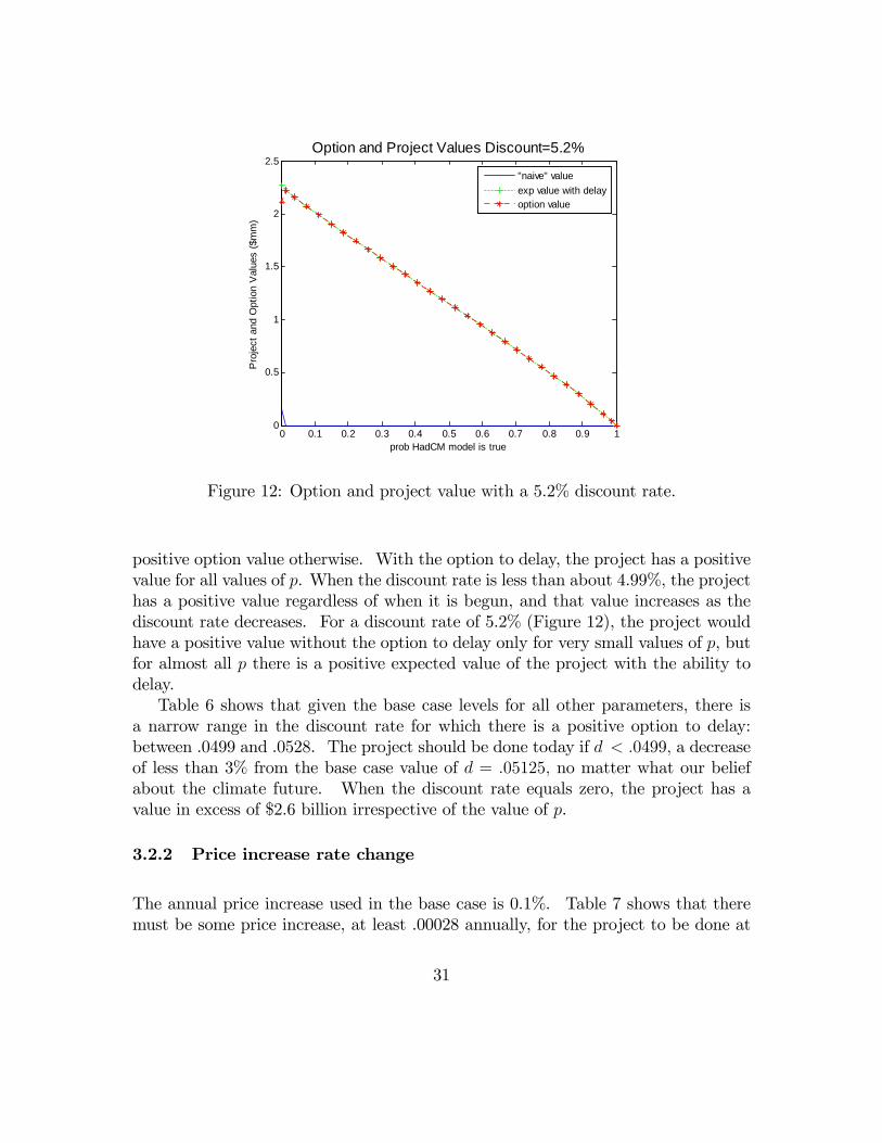
positive option value otherwise. With the option to delay, the project has a positivevalue for all values of p. When the discount rate is less than about 4.99%, the projecthas a positive value regardless of when it is begun, and that value increases as thediscount rate decreases. For a discount rate of 5.2% (Figure 12), the project wouldhave a positive value without the option to delay only for very small values of p, butfor almost all p there is a positive expected value of the project with the ability todelay.Table 6 shows that given the base case levels for all other parameters, there is

a narrow range in the discount rate for which there is a positive option to delay:between .0499 and .0528. The project should be done today if d < :0499; a decreaseof less than 3% from the base case value of d = :05125; no matter what our beliefabout the climate future. When the discount rate equals zero, the project has avalue in excess of $2.6 billion irrespective of the value of p.

3.2.2 Price increase rate change

The annual price increase used in the base case is 0.1%. Table 7 shows that theremust be some price increase, at least .00028 annually, for the project to be done at

31

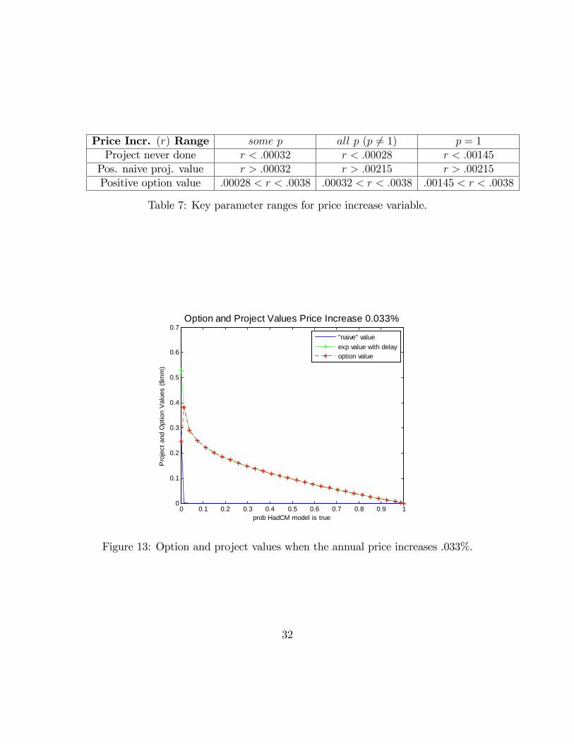
Price Incr. (r) Range some p all p (p 6= 1) p = 1Project never done r < :00032 r < :00028 r < :00145Pos. naive proj. value r > :00032 r > :00215 r > :00215Positive option value :00028 < r < :0038 :00032 < r < :0038 :00145 < r < :0038

Table 7: Key parameter ranges for price increase variable.

0 0.1 0.2 0.3 0.4 0.5 0.6 0.7 0.8 0.9 10

0.1

0.2

0.3

0.4

0.5

0.6

0.7


Pro

ject

and

Opt

ion

Val

ues

($m

m)

Option and Project Values Price Increase 0.033%


Figure 13: Option and project values when the annual price increases .033%.

32

0 0.1 0.2 0.3 0.4 0.5 0.6 0.7 0.8 0.9 10

5

10

15

20

25


Pro

ject

and

Opt

ion

Val

ues

($m

m)

Option and Project Values Price Increase 0.215%


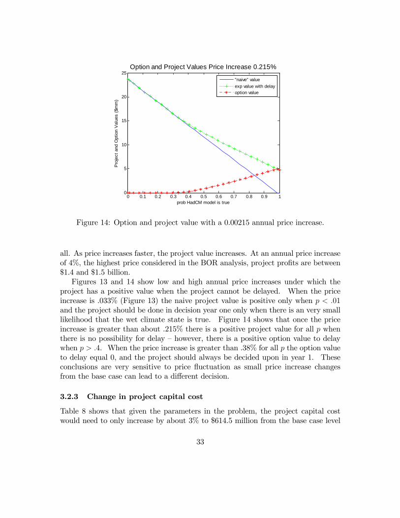
Figure 14: Option and project value with a 0.00215 annual price increase.

all. As price increases faster, the project value increases. At an annual price increaseof 4%, the highest price considered in the BOR analysis, project pro�ts are between$1.4 and $1.5 billion.Figures 13 and 14 show low and high annual price increases under which the

project has a positive value when the project cannot be delayed. When the priceincrease is .033% (Figure 13) the naive project value is positive only when p < :01and the project should be done in decision year one only when there is an very smalllikelihood that the wet climate state is true. Figure 14 shows that once the priceincrease is greater than about .215% there is a positive project value for all p whenthere is no possibility for delay �however, there is a positive option value to delaywhen p > :4. When the price increase is greater than .38% for all p the option valueto delay equal 0, and the project should always be decided upon in year 1. Theseconclusions are very sensitive to price �uctuation as small price increase changesfrom the base case can lead to a di¤erent decision.

3.2.3 Change in project capital cost

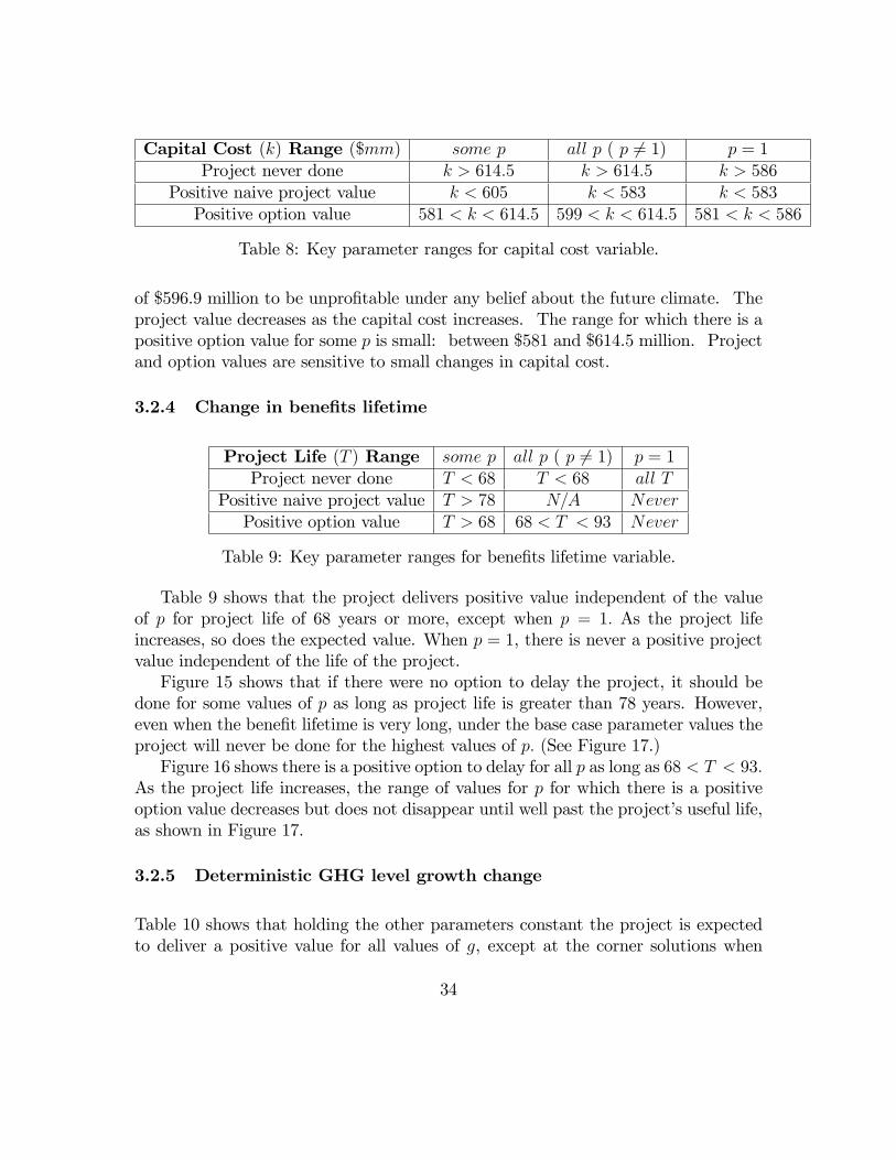
Table 8 shows that given the parameters in the problem, the project capital costwould need to only increase by about 3% to $614.5 million from the base case level

33

Capital Cost (k) Range ($mm) some p all p ( p 6= 1) p = 1Project never done k > 614:5 k > 614:5 k > 586

Positive naive project value k < 605 k < 583 k < 583Positive option value 581 < k < 614:5 599 < k < 614:5 581 < k < 586

Table 8: Key parameter ranges for capital cost variable.

of $596.9 million to be unpro�table under any belief about the future climate. Theproject value decreases as the capital cost increases. The range for which there is apositive option value for some p is small: between $581 and $614.5 million. Projectand option values are sensitive to small changes in capital cost.

3.2.4 Change in bene�ts lifetime

Project Life (T ) Range some p all p ( p 6= 1) p = 1Project never done T < 68 T < 68 all T

Positive naive project value T > 78 N=A NeverPositive option value T > 68 68 < T < 93 Never

Table 9: Key parameter ranges for bene�ts lifetime variable.

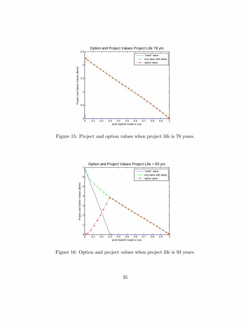
Table 9 shows that the project delivers positive value independent of the valueof p for project life of 68 years or more, except when p = 1: As the project lifeincreases, so does the expected value. When p = 1, there is never a positive projectvalue independent of the life of the project.Figure 15 shows that if there were no option to delay the project, it should be

done for some values of p as long as project life is greater than 78 years. However,even when the bene�t lifetime is very long, under the base case parameter values theproject will never be done for the highest values of p: (See Figure 17.)Figure 16 shows there is a positive option to delay for all p as long as 68 < T < 93:

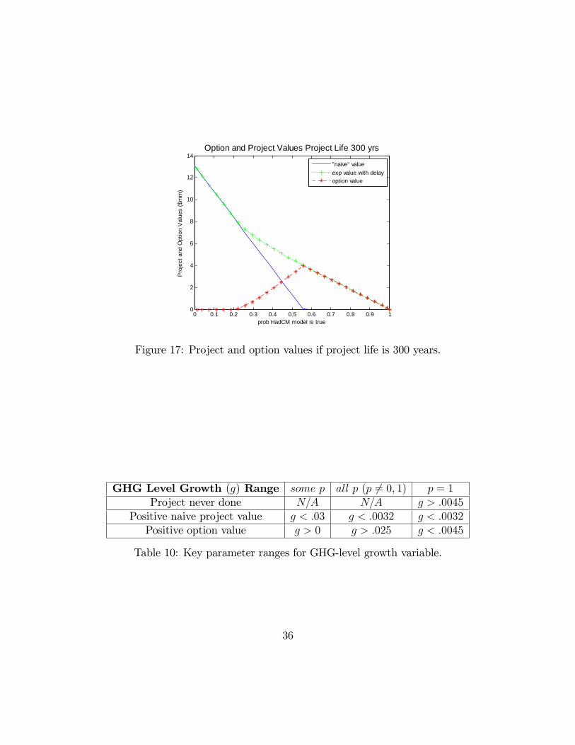
As the project life increases, the range of values for p for which there is a positiveoption value decreases but does not disappear until well past the project�s useful life,as shown in Figure 17.

3.2.5 Deterministic GHG level growth change

Table 10 shows that holding the other parameters constant the project is expectedto deliver a positive value for all values of g, except at the corner solutions when

34

0 0.1 0.2 0.3 0.4 0.5 0.6 0.7 0.8 0.9 10

0.5

1

1.5

2

2.5


Pro

ject

and

Opt

ion

Val

ues

($m

m)

Option and Project Values Project Life 78 yrs


Figure 15: Project and option values when project life is 78 years.

0 0.1 0.2 0.3 0.4 0.5 0.6 0.7 0.8 0.9 10

1

2

3

4

5

6

7


Pro

ject

and

Opt

ion

Val

ues

($m

m)

Option and Project Values Project Life = 93 yrs


Figure 16: Option and project values when project life is 93 years.

35

0 0.1 0.2 0.3 0.4 0.5 0.6 0.7 0.8 0.9 10

2

4

6

8

10

12

14


Pro

ject

and

Opt

ion

Val

ues

($m

m)

Option and Project Values Project Life 300 yrs


Figure 17: Project and option values if project life is 300 years.

GHG Level Growth (g) Range some p all p (p 6= 0; 1) p = 1Project never done N=A N=A g > :0045

Positive naive project value g < :03 g < :0032 g < :0032Positive option value g > 0 g > :025 g < :0045

Table 10: Key parameter ranges for GHG-level growth variable.

36

0 0.1 0.2 0.3 0.4 0.5 0.6 0.7 0.8 0.9 10

1

2

3

4

5

6

7

8

9


Pro

ject

and

Opt

ion

Val

ues

($m

m)

Option and Project Values GHG level growth = .0032


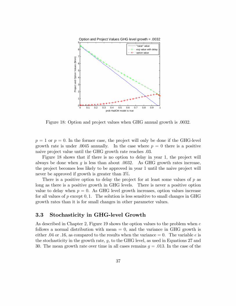
Figure 18: Option and project values when GHG annual growth is .0032.

p = 1 or p = 0: In the former case, the project will only be done if the GHG-levelgrowth rate is under .0045 annually. In the case where p = 0 there is a positivenaive project value until the GHG growth rate reaches .03.Figure 18 shows that if there is no option to delay in year 1, the project will

always be done when g is less than about :0032. As GHG growth rates increase,the project becomes less likely to be approved in year 1 until the naive project willnever be approved if growth is greater than 3%.There is a positive option to delay the project for at least some values of p as

long as there is a positive growth in GHG levels. There is never a positive optionvalue to delay when p = 0. As GHG level growth increases, option values increasefor all values of p except 0; 1. The solution is less sensitive to small changes in GHGgrowth rates than it is for small changes in other parameter values.

3.3 Stochasticity in GHG-level Growth

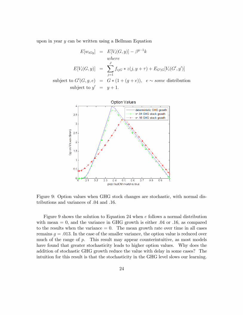
As described in Chapter 2, Figure 19 shows the option values to the problem when efollows a normal distribution with mean = 0, and the variance in GHG growth iseither .04 or .16, as compared to the results when the variance = 0. The variable e isthe stochasticity in the growth rate, g, to the GHG level, as used in Equations 27 and30. The mean growth rate over time in all cases remains g = :013: In the case of the

37

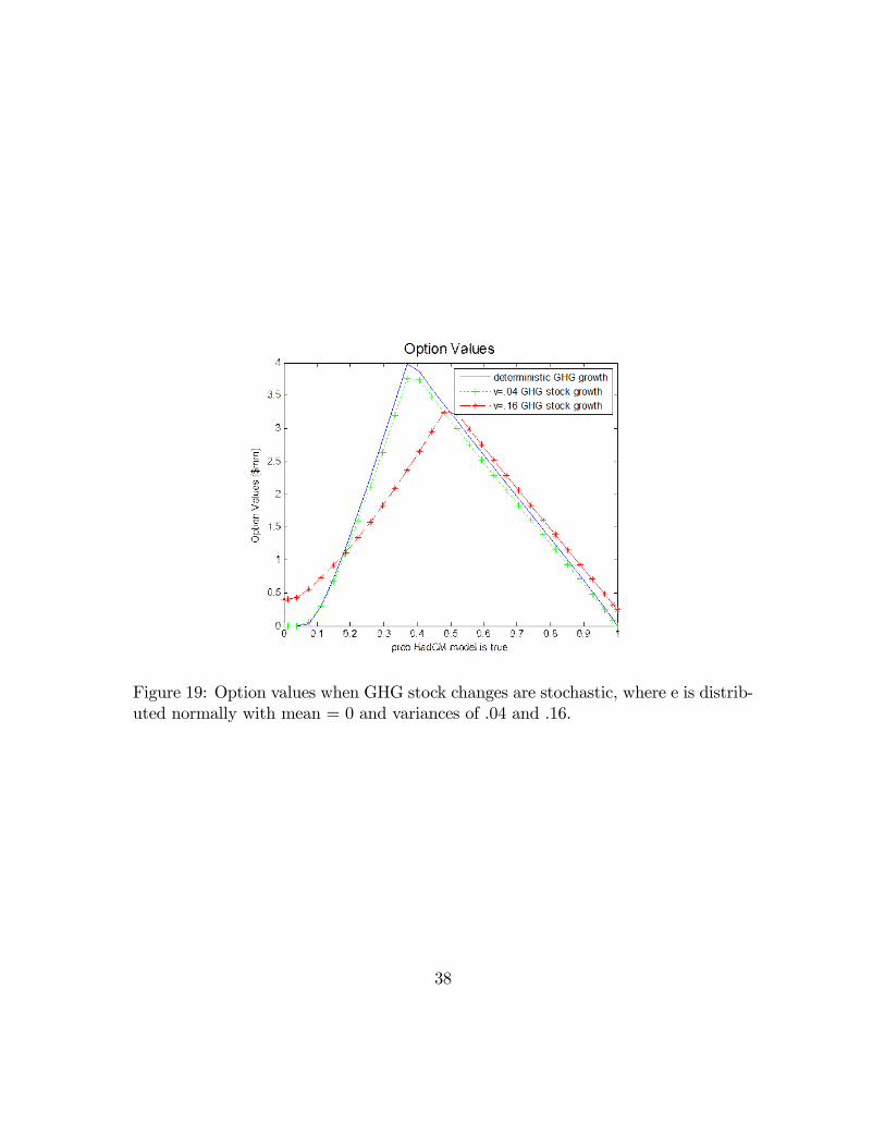
Figure 19: Option values when GHG stock changes are stochastic, where e is distrib-uted normally with mean = 0 and variances of .04 and .16.

38

smaller variance, the option value is reduced over much of the range of p. As stated inChapter 2, this result may appear counterintuitive, as most models have found thatgreater stochasticity leads to higher option values. The intuition for this result is thatthe stochasticity in the GHG level slows our learning. When we observe precipitationrealizations, our estimation of the future changes in precipitation is based not onlyupon the expected precipitation distribution changes given our belief about the trueclimate state, but also on the random speed at which the precipitation distributionwill change. Thus, with GHG stochasticity we cannot anticipate learning as quicklyin the future as we can without. As previously shown, when learning is anticipatedto occur more slowly, the option value of delay diminishes in some cases.With greater stochasticity in GHG growth in Figure 19, (when the variance =

.16) there is still a range of p for which the option value is reduced, but for thehighest and lowest values of p the option value increases. In these cases perhapsthe risk associated with the extreme randomness of the GHG growth outweighs thee¤ect of the slower learning.As a percentage of the base-case value of g = :013, the smaller of these two

variances, :04; is more than 300% or the original parameter value. This large varianceresults in a relatively small change in option value for all p, as shown in Figure 19,suggesting that the problem results are relatively insensitive to GHG stochasticity.

3.4 Discussion

This chapter examines the sensitivity of the conclusions from Chapter 2 to changes inseveral key parameters. I �nd that in the case of discount rates and capital costs, theproject values are very sensitive to small upward parameter value changes. Projectvalues are also sensitive to a small decrease in expected price increases. The projectvalue is less sensitive to changes in the total life of the project, to GHG-level growthand to stochasticity in that growth. Future work might consider how sensitive theproject is to stopping the project once it has begun, for example due to budget cutsor input shortage. The results may vary depending on the probability of such astoppage occurring.

4 Cost-Bene�t Analysis and Decision Making

Dam building dates to antiquity, with the earliest recorded dam dating from 2900BC, a 15 meter masonry structure across the Nile River in Egypt. The oldestdam still in existence is a rock�ll dam built in modern Syria in 1300 BC. Damsbene�tted the ancients in providing �ood control and reservoirs for consistent human

39

and animal water consumption and for irrigation. During the Industrial Revolutionthe construction of dams increased to ful�ll the need for water power. (EncyclopediaBritannica, 1994). From the 20th century dams provided energy in the form ofelectricity. Today there are more than 800,000 dams worldwide, of which over 45,000are taller than a �ve-story building. (World Commission on Dams (WCD), 2000).Leading analysts foresee growing competition for water demand in agriculture,

industry and for drinking water. Each of these uses drain water from natural systems.Populations in water-stressed countries continue to grow, such that by 2025 there areprojected to be a total of 3.5 billion people living in water-stressed areas. Electricitydemand continues to rise, while in 2000 one-third of the earth�s population lackedelectricity. Water for nature is an essential consideration, as freshwater species areincreasingly threatened and wetlands continue to be lost, reducing goods and servicesproduced by aquatic ecosystems upon which many societies depend.The contributions of dams to human development are important and signi�cant,

and dams produce considerable bene�ts for humankind. However, the costs, partic-ularly in environmental and social terms, often have been excessive and unnecessary.Displacement of populations, downstream sacri�ces, environmental destruction andexcessive taxpayer contribution have sometimes outweighed the dam bene�ts. Tak-ing into account all such costs, even when the net bene�ts are positive, distributionof bene�ts and costs are often inequitable, especially when compared to viable alter-natives. Bringing together all a¤ected stakeholders may improve equity and resultin positive resolution of competing interests and con�ict. In addition, it may allowfor the early dismissal of unfavorable projects so that evaluation can focus on themost desirable projects.(WCD, 2000)In analyzing whether to build a dam, there are several questions that must be

answered:1) Is it economically viable? That is, does the economic bene�t outweigh the

economic cost? Economic bene�ts and costs must not only include the actual pricesof the marketable bene�ts and inputs used in construction and management of thedam, but also the values of nonmarket bene�ts and costs and externalities (generallycosts) created by the dam production.2) Are there alternatives that o¤er the same level of net bene�t, but minimize

social and environmental costs? Are there better economic investments availablefor public funds and resources?3) Is it socially equitable? Who will su¤er due to resettlement, loss of livelihood,

loss of local communities and cultures and the transfer of water rights. If the damis not socially equitable, how and to what extent will the losers be compensated bythe winners?

40

4) Is it environmentally sustainable? How will environmental resources be de-pleted, degraded or improved due to the dam? What is the environmental trendover the life of the dam? For example will increased silting cause reduced bene�tsor increased costs over time?We can categorize the bene�ts of a dam into �ve categories: �ood control, on-

demand irrigation, human water consumption, recreation and energy generation.However, assessing the value of any of these bene�ts is not simple. (Hanley andSplash, 1993).Quantifying the costs associated with dams is also complex. There are easily

quanti�able costs, such as that of construction, annual maintenance and operations.There are less easily quanti�able costs, both to human and ecological systems. Hu-mans may be impacted by forced relocation, resulting in cultural harm, or evenannihilation of some cultural systems. Ecosystems may be impacted by the �oodingof areas, resulting in species habitat and other bene�ts of biodiversity destroyed for-ever. Otherwise abundant rivers can be choked, leading to less productive �sheries,degradation of riparian wildlife, changes in temperature of the rivers and growth ofweeds. Anadromous �sh species once supported by rivers that are diverted to thepoint that they no longer reach the ocean are endangered or decimated.As with many capital projects, a dam reallocates the bene�ts from one set of

constituents to another. As stated by the World Commission on Dams (2000):

Dams fundamentally alter rivers and the use of a natural resource, fre-quently entailing a reallocation of bene�ts from local riparian users tonew groups of bene�ciaries at a regional or national level. At the heartof the dams debate are issues of equity, governance, justice and power �issues that underlie the many intractable problems faced by humanity

A most comprehensive and useful method for dam-building evaluation would beto calculate the overall bene�ts to society, calculate the overall costs and �nallyallocate the net bene�ts and costs across winners and losers in society. It wouldconsider how to reallocate some of the net bene�ts of winners to the losers. Sincebene�ts and costs will occur over a long term, often a century or more, a completeanalysis should take into account the uncertainty associated with future pay-o¤ andcost streams �issues like changing future real prices for operations; changing demandfor usage of the energy, recreation or water bene�ts; variances in weather patternsthat result in stochastic annual value; and changes in long-term climate that maya¤ect the value proposition of the project. It would recognize that decision makersvalue the present di¤erently than the future. and thus apply an appropriate discountrate to future expected bene�ts and costs. Finally, the analysis should consider the

41

risk associated with catastrophic events such as earthquakes or �ooding which "tops"the dam.Cost-bene�t analysis (CBA) and it�s close cousin, Cost-e¤ectiveness analysis

(CEA) are two well-recognized economic analysis methods. Yet, there are disagree-ments over the correct approaches for implementing these methods. Two extremeviews of CBA follow, the �rst from Hall (1964, pg 173):

We have begun to grope our way towards a practical concept of economicplanning which may prove in a few year�s time to be as revolutionaryin its policy implications as was the Keynesian revolution in economicsthirty years ago. It also originated, many years ago, with a Cambridgeeconomist: Keynes�contemporary Pigou. It is the concept that we canactually add up the social costs and bene�ts, in money terms, by askingwhat value people would themselves put on them. We can then expressthem as a rate of return on capital, as an ordinary capitalist would, andso determine our investment rationally, from the point of view of thecommunity as a whole, just as the capitalist can now do from his privatepoint of view.

But the practical implementation of such an evaluation system is fraught withproblems. An alternate view expressed by Smithies (1955, pp 344-5) is:

The foregoing discussion leads to two major conclusions: First judgmentplays such an important role in the estimation of bene�t-cost ratios thatlittle signi�cance can be attached to the precise numerical results ob-tained...Second, competition is likely to drive the agencies towards in-creasingly optimistic estimates; and far from resolving the organisationaldi¢ culties, computation of bene�t-cost ratios may in fact make themworse.

These two perspectives show that a CBA can either be considered as the ideal,infallible method of assessing the value of a project or an unreliable waste of timeand e¤ort. (Prest and Turvey, 1965)Other methods to assess the impact of policies include Environmental Impact

Assessments (EIAs), scenario analysis, and risk-e¤ectiveness analysis. These threemethods tend to focus more on the physical information about environmental impactsthan on the pure �nancial costs and rewards. (Hanley and Splash, 1993).In the next section I will focus on CBA and discuss its usefulness and weaknesses.

I will give a history of the method, describe its implementation, and elaborate on

42

areas of controversy. In the following section I will brie�y discuss EnvironmentalImpact Assessments (EIAs) and how they add to the analysis of dam projects. Iwill conclude by discussing recommendations to improve dam analysis.

4.1 Cost-Bene�t Analysis

Cost-bene�t analysis describes the basic �nancial structure used to compare thebene�ts and costs of any large project. I use this section to describe how a CBAis developed for a dam project, largely drawn from Hanley and Splash (1993). Aswill be explained, there are several aspects of CBA that are di¢ cult to quantify. Ienumerate some of them in the last part of this section, and discuss some approachesthat can be taken to address these issues.

4.1.1 Brief history

In 1808, Robert Gallatin, the U.S. Secretary of the Treasury, recommended thatwater-related projects be evaluated by comparing bene�ts to their costs. The Bu-reau of Land Management, created in 1902, was charged with performing economicanalysis of irrigation projects. The Flood Control Act of 1936 provided that bene�tsfor �ood control projects must exceed costs. Continuing improvements to evaluationtechniques occurred, with primary focus on supply-side e¢ ciency in providing a pri-vate good from public projects. Quality management and optimal computer-aidedoperations were incorporated in project analysis, as discussed in Kneese (1964). Theaddition of recreation bene�ts began to be considered, with the early developmentof the travel cost method (Clawson and Knetsch, 1966) to measure the bene�ts ofenvironmental improvement in relation to outdoor recreation. Beginning with theearly 1970s, the e¤ect of projects on public goods such as wildlife, air quality, humanhealth and aesthetics gained consideration, and newer methods to measure these in-tangible bene�ts in addition to the travel cost method, such as contingent valuationand hedonics, began to be considered. In the 1970s and �80s, the importance ofnonuse values, that is value of ecosystems or wildlife that does not directly a¤ecthuman well-being, gained recognition, as examined by Krutilla (1967.) In 1981,Presidential Order 12291 enforced the need for assessment of environmental bene�tsof proposed legislation. In recent years it has become apparent that implementationof CBA is particularly challenging with relation to long-term e¤ects including irre-versibilities, risk and uncertainty. While research continues to consider how thesee¤ects might be incorporated in CBA, practical application of such research is slow.(Hanley and Splash,1993).

43

4.1.2 Steps to analysis

These steps are drawn largely from Hanley and Splash (1993).

De�nition of project This step delineates the reallocation of resources and thepopulation of gainers and losers to be considered. For a dam, water resources aretypically contained in a reservoir, preventing the water from proceeding downstream.Typical gainers when a dam is built are recreational users of lakes, energy producers,agriculture, household users who want to increase the quality or reliability of wateravailability, and communities that are negatively a¤ected by downstream �ooding.The reservoir may create a new lake that can be used for increased recreation. Thewater from the dammay be diverted to be used for irrigation and household use. Thedam may prevent damaging �oods from occurring. The dam may house an energyplant that will create electricity. The losers could be those who must relocate tomake room for a newly �ooded area, riparian users of a river with newly restricted�ows, riparian ecosystems and �sheries. The new reservoir may �ood land that hasother uses, including residential property or sensitive ecosystems. In some caseslarge communities or ecosystems are completely submerged under new reservoirs.Depending on how much the downstream �ow is curtailed, riparian water users maylose access to a water and/or energy sources. Downstream wildlife and ecosystemswill be a¤ected by changes in �ow timing and amount of release, resulting in changesin water temperature, the ability of anadromous �sh to procreate, and the ability ofriver systems to absorb toxins.

Identi�cation of project impacts This step delineates a list of resource, em-ployment, price, tra¢ c, property value, and other impacts that will result from theproject. It should consider additionality and displacement. Additional impacts arenet of other positive impacts that might have occurred without the project. Forexample, without a dam, riparian irrigation may be available. With the dam, theriparian farmers may receive similar irrigation water allocations from the new dam,but this water cannot be considered additional because it was available to the ripar-ian farmer before the dam construction. Displacement refers to other economicallyviable enterprises that will be replaced by the project. For example, a new waterstorage facility may replace land that could be used for agriculture. Or if a reservoiris built that creates a recreational opportunity for �shing and other water sports,the additional value must be calculated to take into consideration the loss of sportand �shery associated with the river that has been curtailed. Also, the reservoirmay lead to lakeside developments that are valuable for developers and taxpayers,

44

but the value of property owned by communities in the �ooded area that is lost mustbe subtracted.

Determination of economically relevant impacts As stated by Hanley andSplash (1993, pg 9) :

The aim of CBA is to select projects which add to the total of socialutility, by increasing the value of consumables and nice views by morethan any associated depletion in the levels of other utility-generatinggoods.

What counts is the maximization of the social welfare function that is derivedby the utility over goods that vary from theater tickets to bananas, nice views andclean air. That is, the bene�ts are a combination of marketable and nonmarketablegoods. CBA is concerned with determining the most e¢ cient projects from a listof alternatives which maximize social welfare. Positive impacts, or bene�ts, areincreases in the quantity or quality of goods that generate positive utility, or decreasesin their prices. Costs are counted as decreases in quantity or quality of such goods,or increases in price. The shadow cost of a non-renewable resource must also beconsidered � that is the cost of preserving a resource for potential use in the future.Quanti�able bene�ts include increasing quantity and quality of consumable goods

that have a market price. Quanti�able costs include the costs of production forsuch goods. Transfer payments should be excluded from such an analysis. Thereare bene�ts and costs that are di¢ cult to quantify using market price, but stillgenerate positive utility, such as clean air or water, unobstructed views and wildlifepreservation, and the shadow cost of non-renewable resources. These may be highlyeconomically relevant to a CBA, but require methods of nonmarket valuation inorder to be adequately accounted for �discussed later in this paper.

Physical quanti�cation of relevant impacts We examine the physical �ows ofthe costs and bene�ts, including timing. For a dam, we might �rst consider howlong the dam will last. With regard to bene�ts, we consider timing and quantities.Bene�ts might include irrigation �ows, residential water �ows, recreational bene�tsand the timing and amount of energy the dam is expected to produce. Costs includethe inputs to building and maintaining the dam, including the amount of resourcessuch as labor and materials. In addition, costs might include the reduction of�sh populations. The estimation of environmental impacts generally necessitatean environmental impact report (EIR.) Calculations of cost and bene�t quantities

45

must take into account uncertainties. While the amount of labor and materials maybe relatively easy to predict, the e¤ect on �sheries may be very di¢ cult to predict.Whenever possible, planners can attach probability distributions to uncertain eventsto arrive at an expected value of a quantity.

Monetary valuation of relevant e¤ects In order to express costs and bene�ts incommon units, the CBA uses money as a convenient device for common valuation.Prices of materials and labor are generated by markets to re�ect relative values,and also their current relative scarcity. To complete the CBA, it is necessary to i)predict future prices for value �ows, ii) correct market prices where necessary andiii) calculate prices for nonmarket valued goods. The prices used in the CBA shouldbe real prices, but should re�ect the relative changes in resource price, such as howrelative prices for cement versus steel may vary in the future. Under scenarios ii) andiii), market prices may not re�ect the true value of a good (that is marginal cost maynot equal price) due to imperfect competition, government intervention in a market,or the absence of a market. In the case of imperfect competition (monopoly oroligopoly), the producer�s marginal cost at the current production quantity re�ectsthe true cost to society of an additional unit, not market price. Where there isgovernment intervention, such as farm subsidies or import taxes, market prices donot re�ect the true cost or bene�t to society of an additional unit. In the case offarm output, producer subsidy equivalents can be calculated and used as the priceestimate of the good.If no market exists for a good, such as for clean air, clean water or biodiversity,

techniques such as contingent valuation, the travel cost method, hedonic pricing,avoided cost and dose-response approaches can be used to estimate marginal socialcost or marginal social bene�t. The valuation of nonmarket goods is a hotly con-tested �eld, and is covered in more detail later in this paper. However, it is generallyagreed that modern CBAmust take environmental costs into account to be thorough.From Randall (1986, pg 193)

No longer can it be claimed that there are overwhelming economic argu-ments for the development option, while the bene�ts of the preservationoption are con�ned to sentiments and emotions existing only in the woollyhead of environmentalists.

Discounting of cost and bene�t �ows The value of a good consumed todaymay di¤er from the value of that good consumed in the future; for example one mayprefer to consume a hamburger today than wait until the following week to consume

46

that same hamburger, even though the price of that hamburger doesn�t change overtime. I may prefer to pay a debt of $100 one year from now rather than today. Inorder to account for this time preference, monetary �ows over time are converted toa measure of their present value by applying a discount rate to future �ows. Thehigher the discount rate, the more the investor prefers the present to the future. Thechoice of discount rate can be controversial. One approach is to use a discount ratethat re�ects the return on investment one would expect to receive should one investin a project with similar risk. However, with respect to natural resources such asclean air and clean water, one can argue that the future value, that is the value ofclean air to our descendants, should not be discounted. By applying a discount rateof only 3% per year, the value of clean air in ten years would be worth only 75% ofits value today. Some would argue that this does not re�ect the true value today ofthe future bene�t. The discount rate is addressed again later in this paper.

Applying the net present value test This test asks whether the net presentvalue gains exceed the net present value costs. If so, the project can be said torepresent an e¢ cient shift in resource allocation that improves social welfare. Thecalculation of the NPV can be expressed as:

NPV =TXt=0

Bt(1 + i)�t +

TXt=0

Ct(1 + i)�t

where Bt represents the bene�t in time period t, i is the discount rate, Ct is the costincurred in time period t, and T is the life of the project. This simple analysis doesnot take into account uncertainty. In order to do so, a probability distribution canbe applied to uncertain bene�ts and costs in order to calculate an expected NPVfor the project. However, in the case of irreversibility and expected learning, thismethod may not result in the optimum decision. This is discussed further later inthis paper.While the expected NPV test may provide a reasonable estimation of overall

social welfare change with the project when there is no anticipation of learning aboutuncertainties over time, it does not give any indication of the allocation of bene�tsand costs between winners and losers. One option to address this failing is to weightimpacts according to income, thereby taking into account the fact that willingness topay (WTP) will di¤er depending on the wealth of those a¤ected. For example, if theimpact a¤ecting a low-income group is -$1 million, and a high-income group wouldreceive a $2 million impact, the net impact to society is $1 million and the projectwould be acceptable. But perhaps the low-income group would starve if they paid

47

$1 million, but the high-income group could easily borrow $2 million at low interestrates. To remedy this issue, the low-income group�s loss could be weighted higher,say at 75%, leading to a net impact of -$.25 million, and the project would not bedone. Re-weighting the impacts according to income or some other factor is rarelypracticed at the public agency level. This kind of inequity demonstrates why CBAis rarely the sole input to decisions a¤ecting di¤erent groups.

Sensitivity analysis This test explores how the NPV of a project changes shoulda single input in the calculations change. This kind of analysis is helpful as a wayto address the fact that some future �ows of bene�ts or costs are uncertain. Forexample, with respect to a dam, future weather patterns are unknown and may a¤ectthe water available for storage, irrigation and electricity generation. The real priceof bene�t �ows or the costs may change. A small increase in the discount rate maycause the project value to be negative. The true life span of the project may bemore or less than that used in the base NPV analysis, and if too short the projectNPV may no longer be positive. The key parameters to be analyzed should be thosequantities and qualities that are uncertain and that could either vary considerablyor could have a large a¤ect on the project given a small variance.

4.1.3 Problem areas using CBA

In this section I address several di¢ culties in deriving an accurate net present valueanalysis using CBA, most of which have already been mentioned.1) The valuation of nonmarket goods such as habitat, clean air, views or ecosys-

tems.2) Ecosystem complexity. Can society predict the full cost of destruction of

a rain forest, including lost species, lost plant life that could have been used formedicinal purposes, value of plant carbon capture, e¤ect on neighboring ecosystems,etc.?3) The choice of discount rate. How should we value what is permanently lost

to future generations, and would they approve our placing less value on their bene�tsthan on ours?4) Industrial capture. Since CBA is often performed by institutions that will

bene�t from the projects that they are analyzing, can we rely on their objectiveassessments of bene�ts, costs and risks?5) Uncertainty and irreversibility with anticipated learning. How will these be

accounted for in a CBA?6) Allocation issues. Will the gainers compensate the losers?

48

Nonmarket valuation Market prices do not always re�ect the value of goods. Ifone were on a desert island and could choose between a day�s worth of fresh water ora large amount of gold, one would choose the good that has a market value close to$0. While not traded in a marketplace, air, water and land quality and availabilityfor use have value. Our health and our ability to enjoy our environment, throughhaving clear views or enjoying recreation, are also amenities that are not readilyevaluated through markets. The quality of each of these goods can change due tochoices made by society, but cannot be decided upon unilaterally by individuals.Nonmarket costs or bene�ts can a¤ect humans in a variety of ways. Focusing

on pollution costs, in some cases pollutants to water, air and land may a¤ect humanhealth or wealth directly and equally. For example, all of the residents of Los Angelescounty experience the negative e¤ects of air pollution. In other cases, di¤erent usersof a given nonmarket good may not experience the same level of such good. Forexample, people who live close to trash dumps incur more costs in terms of healthrisks and a negative environment than those who live further away. Other instancesof pollution may a¤ect far away ecosystems that may indirectly a¤ect humans (themelting of the arctic ice sheets that leads to rising sea levels) or may never directlya¤ect humans (the garbage left in space from orbiters and satellites.)Economists attempt to maximize a social welfare function that describes the

aggregate well-being of individuals. Individual preferences are described by theirwillingness to pay for gains or accept payment for losses of goods, including nonmar-ket goods. The compensating surplus for an environmental good is the maximumamount a person would pay to not give up an improvement to that good �or willing-ness to pay (WTP). For example, if there is a creek that is polluted, how much willeach person who lives along that creek pay in order to clean it up? The equivalentsurplus is the minimum sum of money a person needs in order to forego the improve-ment, or willingness to accept (WTA). For example, if the government has alreadyplanned to improve the creek water quality, WTA measures how much money eachresident would be willing to accept in order forego such improvement. Each mea-sure assumes that an environmental good could be substituted for by some amountof money. The decision about which measurement to use depends on the type ofproblem.Whether economists are measuring WTP or WTA, they need some way other

than market prices to assess values for nonmarket goods. There are two types ofmethods used to estimate such values: stated preferences and revealed preferences.Revealed preference methods rely on how actual purchases of market valued goodsre�ect the value of nonmarket goods. Stated preference methods rely primarily onsurvey data in which responders place monetary values on nonmarket goods.

49

Revealed preference methods allow researchers to infer values of nonmarket goodsthrough the prices paid for market goods that include nonmarket amenities. Revealedpreference methods draw statistical inferences on values from actual choices peoplemake within markets. Although we do not explicitly purchase nonmarket goods,we do purchase other goods for which demand is related to nonmarket goods. Forexample, we may choose to recreate where there is clear air, clean water, forests, �shand other environmental amenities. Or, we may choose to buy a home that hasaccess to park areas, lakes or attractive views. Prices of homes or recreational areasmay be higher when such amenities are available compared to when they are not.There are four commonly used revealed preference methods: travel cost, hedonics,defensive behavior and damage costs. Travel costs are used to estimate values forrecreational usage changes when environmental quality changes. Hedonic modelsanalyze how home or other property prices change when they are close or far fromenvironmental amenities. Defensive behavior models analyze what people are willingto pay to reduce risk of exposure to disamenities such as pollution. The damage costmethod measures the costs associated with environmental contamination. (Boyle,2003)Stated preference methods use carefully worded surveys to rank preferences mon-

etarily or ordinally. Some skepticism exists for stated preference methods becauseof a concern that people will not or cannot answer valuation questions truthfully.Stated preference methods can be used where there is no linkage between marketand nonmarket goods, an advantage over revealed preference methods. This ad-vantage is particularly useful in the case of nonuse amenities, such as wildernessor species preservation. There are three methods for stated preference valuation:attribute-based methods, paired comparison and contingent valuation. The con-tingent valuation method was designed to measure monetary value, generally of asingle good. Survey takers may be asked "How much would you be willing to pay toremove the sludge from the creek near your property?" The criticism is that surveytakers may not actually pay that amount if required to do so. The other two meth-ods were originally designed for ordered preferences, but have since been adapted formonetary valuation. The paired comparison method asks survey takers to comparevalues of numerous goods, and by including money as one good results in monetaryvaluation. The attribute-based method compares the value of similar goods thatdi¤er in the level of certain assets to be valued. Once again, by including monetarycost of an attribute, monetary valuation can be achieved. (Brown, 2003)

Ecosystem complexity CBA of a project that reduces or enhances ecosystemcomplexity must attempt to quantify the value of ecosystem services that bene�t

50

humans. Ecosystem complexity provides a challenge in bene�t evaluation. Fisher,et.al. (2008) suggest three criteria to be used to evaluate the human bene�t forecosystem services. 1) The marginal bene�t of increasing or decreasing a protectedecosystem area or species should be quanti�ed and considered in a CBA. For example,the pollination services provided by a small forest next to a co¤ee plantation from thebirds and insects should be weighed against the increased production from arable landthat would result from the forest�s destruction. If the contribution of the pollinatorsis reduced along with the forest, the marginal bene�t could be negative. 2) The safeminimum standard of ecosystem or structure is that below which the ecosystem willchange nonlinearly and perhaps irrecoverably. There is a high level of uncertaintyabout where the minimum quantity of ecosystem structure and process (includingdiversity, populations, interactions, etc.) exists. For example, the otter populationdecline in the Aleutians led to an increase in the sea urchin biomass, resulting in acollapse of the otherwise healthy kelp system. 3) There is a demand for ecosystemservices that is not re�ected in market prices. See the above discussion on nonmarketvaluation. Fisher et.al. (2008) conduct a thorough review of literature addressingthe economic bene�t of environmental services. They point to many studies thatnote that the market under-provides ecosystem services. Ecosystem attributes thatonly indirectly bene�t humans may have value as a nonuse good, but their bene�tsmay be di¢ cult to quantify.

Discount rate Howarth and Norgaard (1993) investigate the relationship betweenintergenerational asset transfers and the choice of the discount rate for use in cost-bene�t analysis in a model of a competitive overlapping generations economy con-strained by a socially managed exhaustible resource. They �nd that if the discountrate is set equal to the market rate of interest, and there are no distortions in cap-ital markets and that all agents hold perfect foresight, cost-bene�t techniques willresult in a Pareto e¢ cient resource allocation. But since the path of the interestrate depends on the level of intergenerational transfers, cost-bene�t techniques donot ensure a socially desirable distribution of welfare between generations; a socialoptimum will result only if intergenerational transfers are properly chosen and en-forced. In general, there will be an under distribution of assets from the current tofuture generations. Their conclusion is that CBA is at best a partial criterion topolicy formulation that should be used only in conjunction with ethical principlesthat de�ne the proper distribution of welfare between present and future generations.Ackerman (2009) comments on the conclusion of The Stern Review, released in

2006 by a team headed by Sir Nicolas Stern who reviewed the economics of climatechange at the request of the British government. Ackerman points out there are

51

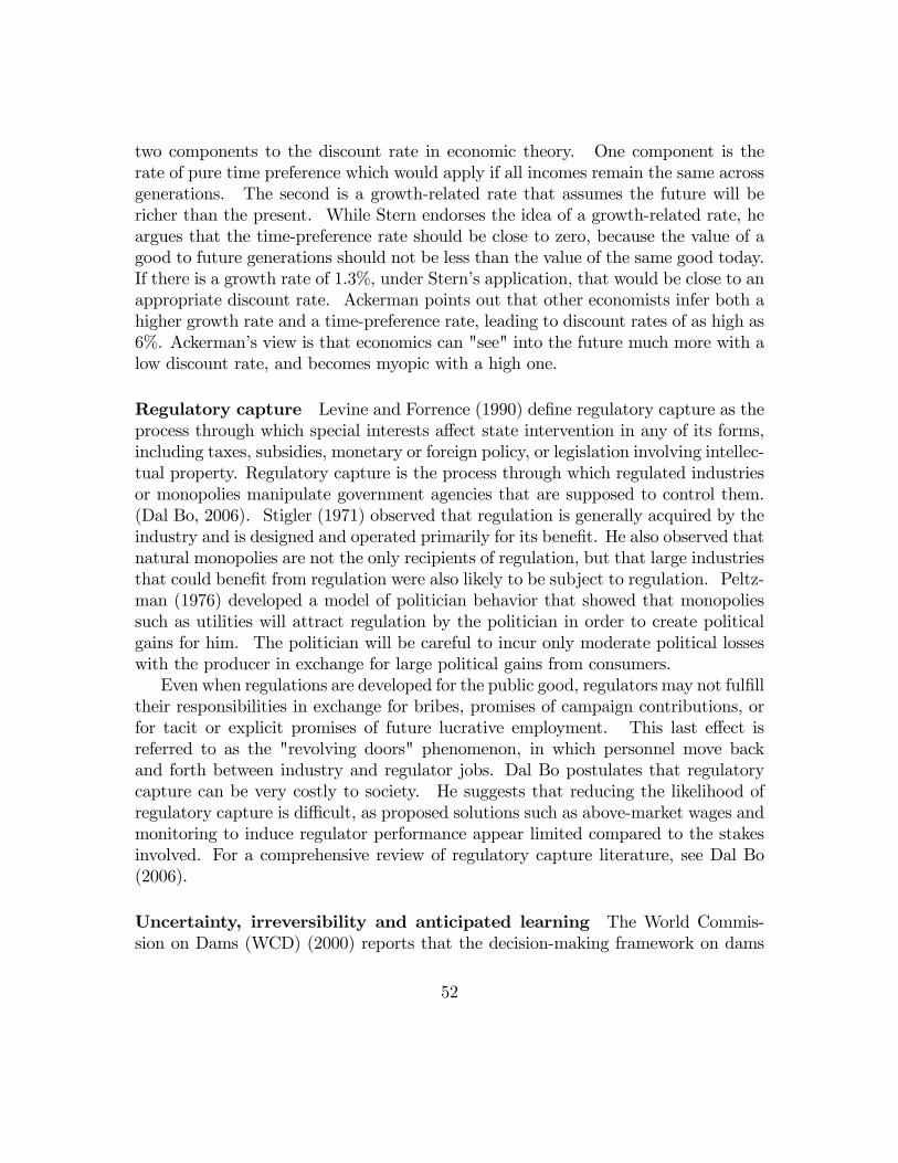
two components to the discount rate in economic theory. One component is therate of pure time preference which would apply if all incomes remain the same acrossgenerations. The second is a growth-related rate that assumes the future will bericher than the present. While Stern endorses the idea of a growth-related rate, heargues that the time-preference rate should be close to zero, because the value of agood to future generations should not be less than the value of the same good today.If there is a growth rate of 1.3%, under Stern�s application, that would be close to anappropriate discount rate. Ackerman points out that other economists infer both ahigher growth rate and a time-preference rate, leading to discount rates of as high as6%. Ackerman�s view is that economics can "see" into the future much more with alow discount rate, and becomes myopic with a high one.

Regulatory capture Levine and Forrence (1990) de�ne regulatory capture as theprocess through which special interests a¤ect state intervention in any of its forms,including taxes, subsidies, monetary or foreign policy, or legislation involving intellec-tual property. Regulatory capture is the process through which regulated industriesor monopolies manipulate government agencies that are supposed to control them.(Dal Bo, 2006). Stigler (1971) observed that regulation is generally acquired by theindustry and is designed and operated primarily for its bene�t. He also observed thatnatural monopolies are not the only recipients of regulation, but that large industriesthat could bene�t from regulation were also likely to be subject to regulation. Peltz-man (1976) developed a model of politician behavior that showed that monopoliessuch as utilities will attract regulation by the politician in order to create politicalgains for him. The politician will be careful to incur only moderate political losseswith the producer in exchange for large political gains from consumers.Even when regulations are developed for the public good, regulators may not ful�ll

their responsibilities in exchange for bribes, promises of campaign contributions, orfor tacit or explicit promises of future lucrative employment. This last e¤ect isreferred to as the "revolving doors" phenomenon, in which personnel move backand forth between industry and regulator jobs. Dal Bo postulates that regulatorycapture can be very costly to society. He suggests that reducing the likelihood ofregulatory capture is di¢ cult, as proposed solutions such as above-market wages andmonitoring to induce regulator performance appear limited compared to the stakesinvolved. For a comprehensive review of regulatory capture literature, see Dal Bo(2006).

Uncertainty, irreversibility and anticipated learning The World Commis-sion on Dams (WCD) (2000) reports that the decision-making framework on dams

52

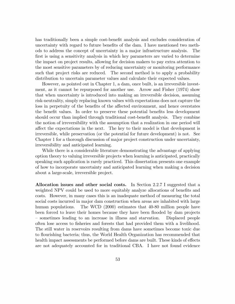
has traditionally been a simple cost-bene�t analysis and excludes consideration ofuncertainty with regard to future bene�ts of the dam. I have mentioned two meth-ods to address the concept of uncertainty in a major infrastructure analysis. The�rst is using a sensitivity analysis in which key parameters are varied to determinethe impact on project results, allowing for decision makers to pay extra attention tothe most sensitive parameters by of reducing uncertainty or monitoring performancesuch that project risks are reduced. The second method is to apply a probabilitydistribution to uncertain parameter values and calculate their expected values.However, as pointed out in Chapter 1, a dam, once built, is an irreversible invest-

ment, as it cannot be repurposed for another use. Arrow and Fisher (1974) showthat when uncertainty is introduced into making an irreversible decision, assumingrisk-neutrality, simply replacing known values with expectations does not capture theloss in perpetuity of the bene�ts of the a¤ected environment, and hence overstatesthe bene�t values. In order to preserve these potential bene�ts less developmentshould occur than implied through traditional cost-bene�t analysis. They combinethe notion of irreversibility with the assumption that a realization in one period willa¤ect the expectations in the next. The key to their model is that development isirreversible, while preservation (or the potential for future development) is not. SeeChapter 1 for a thorough discussion of major project construction under uncertainty,irreversibility and anticipated learning.While there is a considerable literature demonstrating the advantage of applying

option theory to valuing irreversible projects when learning is anticipated, practicallyspeaking such application is rarely practiced. This dissertation presents one exampleof how to incorporate uncertainty and anticipated learning when making a decisionabout a large-scale, irreversible project.

Allocation issues and other social costs. In Section 2.2.7 I suggested that aweighted NPV could be used to more equitably analyze allocations of bene�ts andcosts. However, in many cases this is an inadequate method of measuring the totalsocial costs incurred in major dam construction when areas are inhabited with largehuman populations. The WCD (2000) estimates that 40-80 million people havebeen forced to leave their homes because they have been �ooded by dam projects� sometimes leading to an increase in illness and starvation. Displaced peopleoften lose access to �sheries and forests that had provided them with a livelihood.The still water in reservoirs resulting from dams have sometimes become toxic dueto �ourishing bacteria; thus, the World Health Organization has recommended thathealth impact assessments be performed before dams are built. These kinds of e¤ectsare not adequately accounted for in traditional CBA. I have not found evidence

53

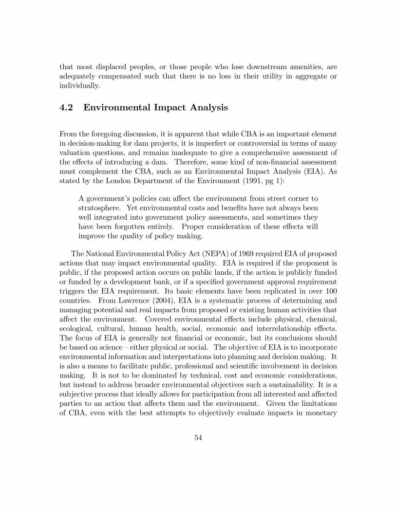
that most displaced peoples, or those people who lose downstream amenities, areadequately compensated such that there is no loss in their utility in aggregate orindividually.

4.2 Environmental Impact Analysis

From the foregoing discussion, it is apparent that while CBA is an important elementin decision-making for dam projects, it is imperfect or controversial in terms of manyvaluation questions, and remains inadequate to give a comprehensive assessment ofthe e¤ects of introducing a dam. Therefore, some kind of non-�nancial assessmentmust complement the CBA, such as an Environmental Impact Analysis (EIA). Asstated by the London Department of the Environment (1991, pg 1):

A government�s policies can a¤ect the environment from street corner tostratosphere. Yet environmental costs and bene�ts have not always beenwell integrated into government policy assessments, and sometimes theyhave been forgotten entirely. Proper consideration of these e¤ects willimprove the quality of policy making.

The National Environmental Policy Act (NEPA) of 1969 required EIA of proposedactions that may impact environmental quality. EIA is required if the proponent ispublic, if the proposed action occurs on public lands, if the action is publicly fundedor funded by a development bank, or if a speci�ed government approval requirementtriggers the EIA requirement. Its basic elements have been replicated in over 100countries. From Lawrence (2004), EIA is a systematic process of determining andmanaging potential and real impacts from proposed or existing human activities thata¤ect the environment. Covered environmental e¤ects include physical, chemical,ecological, cultural, human health, social, economic and interrelationship e¤ects.The focus of EIA is generally not �nancial or economic, but its conclusions shouldbe based on science �either physical or social. The objective of EIA is to incorporateenvironmental information and interpretations into planning and decision making. Itis also a means to facilitate public, professional and scienti�c involvement in decisionmaking. It is not to be dominated by technical, cost and economic considerations,but instead to address broader environmental objectives such a sustainability. It is asubjective process that ideally allows for participation from all interested and a¤ectedparties to an action that a¤ects them and the environment. Given the limitationsof CBA, even with the best attempts to objectively evaluate impacts in monetary

54

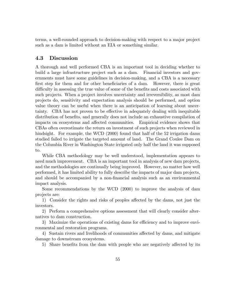
terms, a well-rounded approach to decision-making with respect to a major projectsuch as a dam is limited without an EIA or something similar.

4.3 Discussion

A thorough and well performed CBA is an important tool in deciding whether tobuild a large infrastructure project such as a dam. Financial investors and gov-ernments must have some guidelines in decision-making, and a CBA is a necessary�rst step for them and for other bene�ciaries of a dam. However, there is greatdi¢ culty in assessing the true value of some of the bene�ts and costs associated withsuch projects. When a project involves uncertainty and irreversibility, as most damprojects do, sensitivity and expectation analysis should be performed, and optionvalue theory can be useful when there is an anticipation of learning about uncer-tainty. CBA has not proven to be e¤ective in adequately dealing with inequitabledistribution of bene�ts, and generally does not include an exhaustive compilation ofimpacts on ecosystems and a¤ected communities. Empirical evidence shows thatCBAs often overestimate the return on investment of such projects when reviewed inhindsight. For example, the WCD (2000) found that half of the 52 irrigation damsstudied failed to irrigate the targeted amount of land. The Grand Coulee Dam onthe Columbia River in Washington State irrigated only half the land it was supposedto.While CBA methodology may be well understood, implementation appears to

need much improvement. CBA is an important tool in analysis of new dam projects,and the methodologies are continually being improved. However, no matter how wellperformed, it has limited ability to fully describe the impacts of major dam projects,and should be accompanied by a non-�nancial analysis such as an environmentalimpact analysis.Some recommendations by the WCD (2000) to improve the analysis of dam

projects are:1) Consider the rights and risks of peoples a¤ected by the dams, not just the

investors.2) Perform a comprehensive options assessment that will clearly consider alter-

natives to dam construction.3) Maximize the operations of existing dams for e¢ ciency and to improve envi-

ronmental and restoration programs.4) Sustain rivers and livelihoods of communities a¤ected by dams, and mitigate

damage to downstream ecosystems.5) Share bene�ts from the dam with people who are negatively a¤ected by its

55

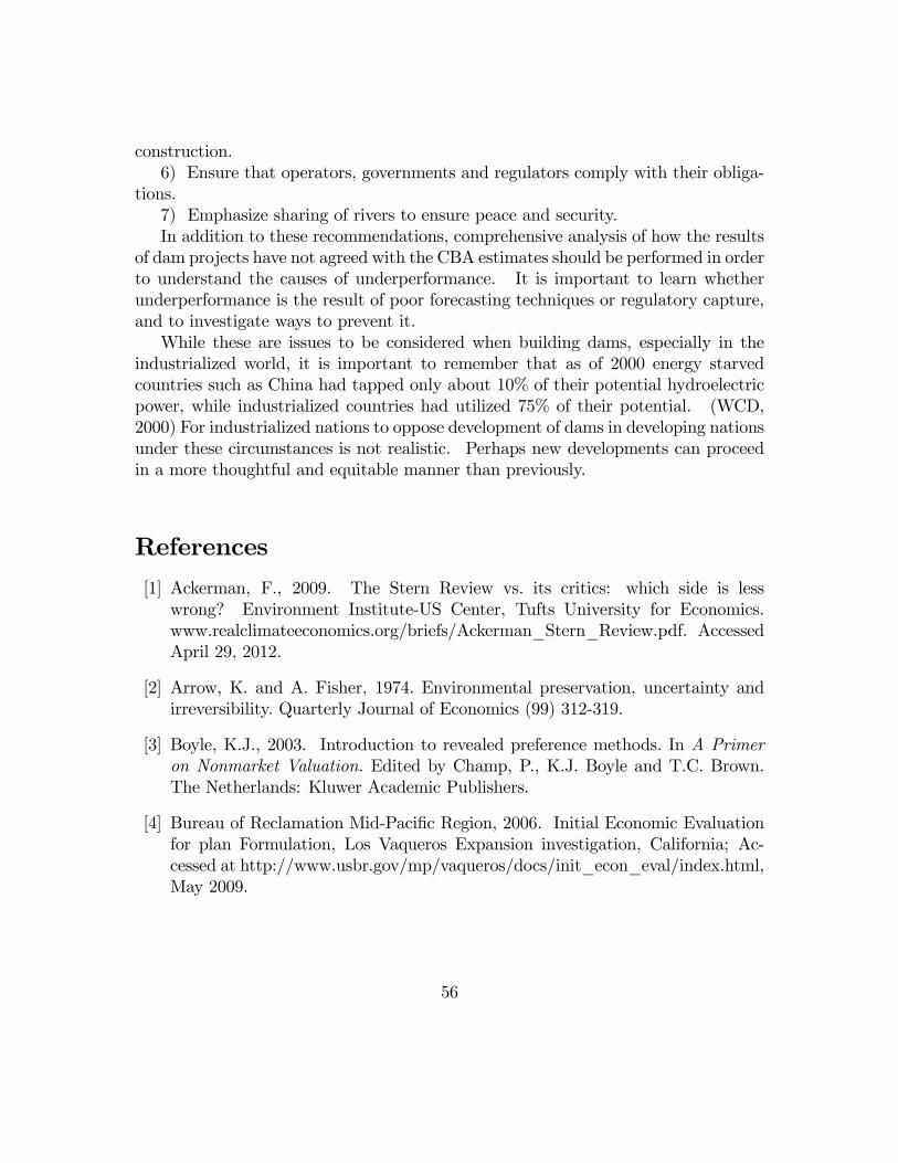
construction.6) Ensure that operators, governments and regulators comply with their obliga-

tions.7) Emphasize sharing of rivers to ensure peace and security.In addition to these recommendations, comprehensive analysis of how the results

of dam projects have not agreed with the CBA estimates should be performed in orderto understand the causes of underperformance. It is important to learn whetherunderperformance is the result of poor forecasting techniques or regulatory capture,and to investigate ways to prevent it.While these are issues to be considered when building dams, especially in the

industrialized world, it is important to remember that as of 2000 energy starvedcountries such as China had tapped only about 10% of their potential hydroelectricpower, while industrialized countries had utilized 75% of their potential. (WCD,2000) For industrialized nations to oppose development of dams in developing nationsunder these circumstances is not realistic. Perhaps new developments can proceedin a more thoughtful and equitable manner than previously.

References

[1] Ackerman, F., 2009. The Stern Review vs. its critics: which side is lesswrong? Environment Institute-US Center, Tufts University for Economics.www.realclimateeconomics.org/briefs/Ackerman_Stern_Review.pdf. AccessedApril 29, 2012.

[2] Arrow, K. and A. Fisher, 1974. Environmental preservation, uncertainty andirreversibility. Quarterly Journal of Economics (99) 312-319.

[3] Boyle, K.J., 2003. Introduction to revealed preference methods. In A Primeron Nonmarket Valuation. Edited by Champ, P., K.J. Boyle and T.C. Brown.The Netherlands: Kluwer Academic Publishers.

[4] Bureau of Reclamation Mid-Paci�c Region, 2006. Initial Economic Evaluationfor plan Formulation, Los Vaqueros Expansion investigation, California; Ac-cessed at http://www.usbr.gov/mp/vaqueros/docs/init_econ_eval/index.html,May 2009.

56

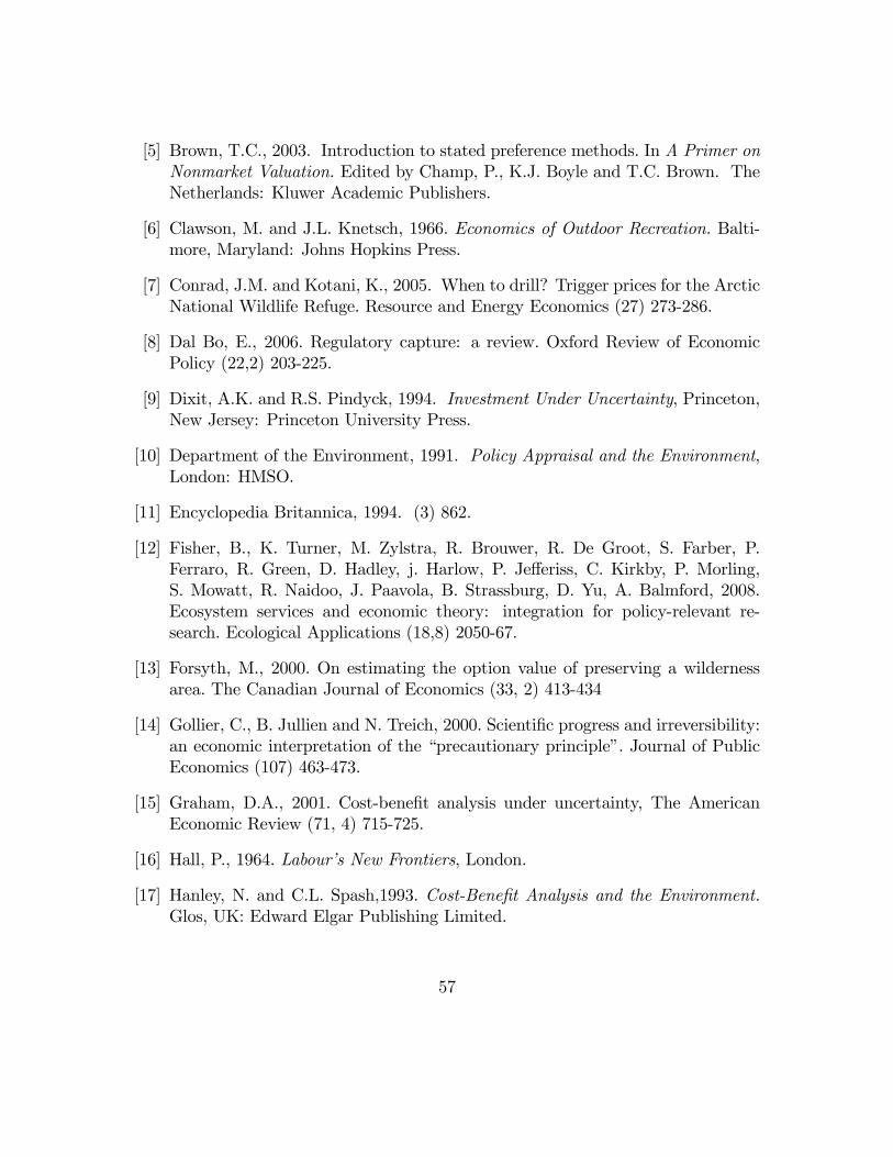
[5] Brown, T.C., 2003. Introduction to stated preference methods. In A Primer onNonmarket Valuation. Edited by Champ, P., K.J. Boyle and T.C. Brown. TheNetherlands: Kluwer Academic Publishers.

[6] Clawson, M. and J.L. Knetsch, 1966. Economics of Outdoor Recreation. Balti-more, Maryland: Johns Hopkins Press.

[7] Conrad, J.M. and Kotani, K., 2005. When to drill? Trigger prices for the ArcticNational Wildlife Refuge. Resource and Energy Economics (27) 273-286.

[8] Dal Bo, E., 2006. Regulatory capture: a review. Oxford Review of EconomicPolicy (22,2) 203-225.

[9] Dixit, A.K. and R.S. Pindyck, 1994. Investment Under Uncertainty, Princeton,New Jersey: Princeton University Press.

[10] Department of the Environment, 1991. Policy Appraisal and the Environment,London: HMSO.

[11] Encyclopedia Britannica, 1994. (3) 862.

[12] Fisher, B., K. Turner, M. Zylstra, R. Brouwer, R. De Groot, S. Farber, P.Ferraro, R. Green, D. Hadley, j. Harlow, P. Je¤eriss, C. Kirkby, P. Morling,S. Mowatt, R. Naidoo, J. Paavola, B. Strassburg, D. Yu, A. Balmford, 2008.Ecosystem services and economic theory: integration for policy-relevant re-search. Ecological Applications (18,8) 2050-67.

[13] Forsyth, M., 2000. On estimating the option value of preserving a wildernessarea. The Canadian Journal of Economics (33, 2) 413-434

[14] Gollier, C., B. Jullien and N. Treich, 2000. Scienti�c progress and irreversibility:an economic interpretation of the �precautionary principle�. Journal of PublicEconomics (107) 463-473.

[15] Graham, D.A., 2001. Cost-bene�t analysis under uncertainty, The AmericanEconomic Review (71, 4) 715-725.

[16] Hall, P., 1964. Labour�s New Frontiers, London.

[17] Hanley, N. and C.L. Spash,1993. Cost-Bene�t Analysis and the Environment.Glos, UK: Edward Elgar Publishing Limited.

57

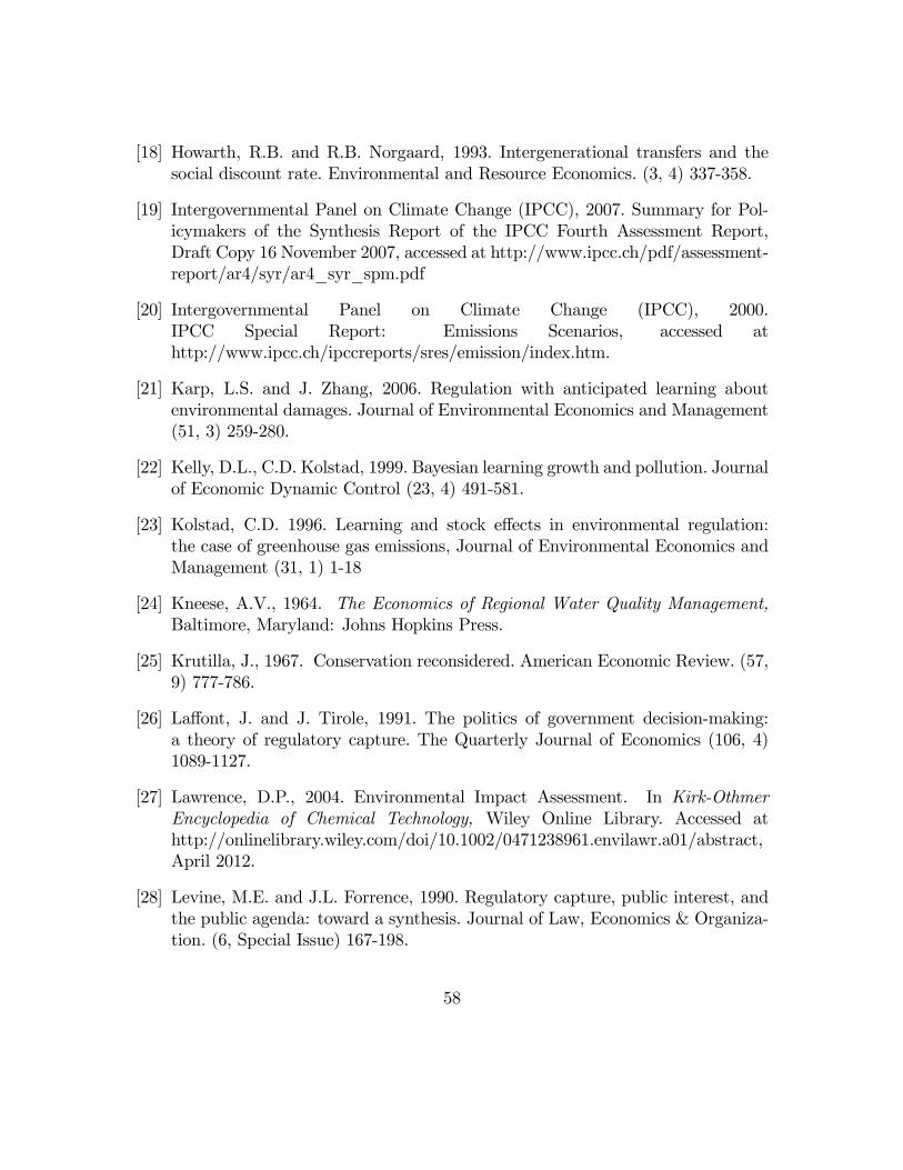
[18] Howarth, R.B. and R.B. Norgaard, 1993. Intergenerational transfers and thesocial discount rate. Environmental and Resource Economics. (3, 4) 337-358.

[19] Intergovernmental Panel on Climate Change (IPCC), 2007. Summary for Pol-icymakers of the Synthesis Report of the IPCC Fourth Assessment Report,Draft Copy 16 November 2007, accessed at http://www.ipcc.ch/pdf/assessment-report/ar4/syr/ar4_syr_spm.pdf

[20] Intergovernmental Panel on Climate Change (IPCC), 2000.IPCC Special Report: Emissions Scenarios, accessed athttp://www.ipcc.ch/ipccreports/sres/emission/index.htm.

[21] Karp, L.S. and J. Zhang, 2006. Regulation with anticipated learning aboutenvironmental damages. Journal of Environmental Economics and Management(51, 3) 259-280.

[22] Kelly, D.L., C.D. Kolstad, 1999. Bayesian learning growth and pollution. Journalof Economic Dynamic Control (23, 4) 491-581.

[23] Kolstad, C.D. 1996. Learning and stock e¤ects in environmental regulation:the case of greenhouse gas emissions, Journal of Environmental Economics andManagement (31, 1) 1-18

[24] Kneese, A.V., 1964. The Economics of Regional Water Quality Management,Baltimore, Maryland: Johns Hopkins Press.

[25] Krutilla, J., 1967. Conservation reconsidered. American Economic Review. (57,9) 777-786.

[26] La¤ont, J. and J. Tirole, 1991. The politics of government decision-making:a theory of regulatory capture. The Quarterly Journal of Economics (106, 4)1089-1127.

[27] Lawrence, D.P., 2004. Environmental Impact Assessment. In Kirk-OthmerEncyclopedia of Chemical Technology, Wiley Online Library. Accessed athttp://onlinelibrary.wiley.com/doi/10.1002/0471238961.envilawr.a01/abstract,April 2012.

[28] Levine, M.E. and J.L. Forrence, 1990. Regulatory capture, public interest, andthe public agenda: toward a synthesis. Journal of Law, Economics & Organiza-tion. (6, Special Issue) 167-198.

58

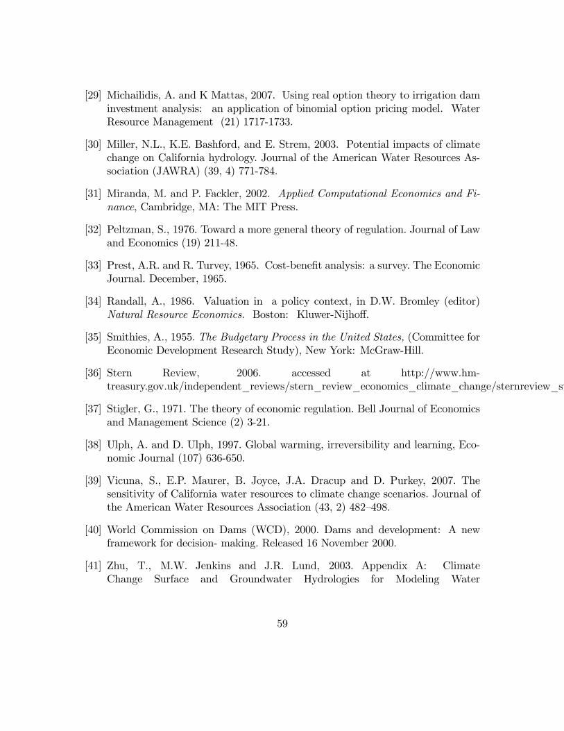
[29] Michailidis, A. and K Mattas, 2007. Using real option theory to irrigation daminvestment analysis: an application of binomial option pricing model. WaterResource Management (21) 1717-1733.

[30] Miller, N.L., K.E. Bashford, and E. Strem, 2003. Potential impacts of climatechange on California hydrology. Journal of the American Water Resources As-sociation (JAWRA) (39, 4) 771-784.

[31] Miranda, M. and P. Fackler, 2002. Applied Computational Economics and Fi-nance, Cambridge, MA: The MIT Press.

[32] Peltzman, S., 1976. Toward a more general theory of regulation. Journal of Lawand Economics (19) 211-48.

[33] Prest, A.R. and R. Turvey, 1965. Cost-bene�t analysis: a survey. The EconomicJournal. December, 1965.

[34] Randall, A., 1986. Valuation in a policy context, in D.W. Bromley (editor)Natural Resource Economics. Boston: Kluwer-Nijho¤.

[35] Smithies, A., 1955. The Budgetary Process in the United States, (Committee forEconomic Development Research Study), New York: McGraw-Hill.

[36] Stern Review, 2006. accessed at http://www.hm-treasury.gov.uk/independent_reviews/stern_review_economics_climate_change/sternreview_summary.cfm

[37] Stigler, G., 1971. The theory of economic regulation. Bell Journal of Economicsand Management Science (2) 3-21.

[38] Ulph, A. and D. Ulph, 1997. Global warming, irreversibility and learning, Eco-nomic Journal (107) 636-650.

[39] Vicuna, S., E.P. Maurer, B. Joyce, J.A. Dracup and D. Purkey, 2007. Thesensitivity of California water resources to climate change scenarios. Journal ofthe American Water Resources Association (43, 2) 482�498.

[40] World Commission on Dams (WCD), 2000. Dams and development: A newframework for decision- making. Released 16 November 2000.

[41] Zhu, T., M.W. Jenkins and J.R. Lund, 2003. Appendix A: ClimateChange Surface and Groundwater Hydrologies for Modeling Water

59

Supply Management. Department of Civil and Environmental Engi-neering, University of California-Davis, Davis, California. Available athttp://cee.engr.ucdavis.edu/faculty/lund/CALVIN/ReportCEC/AppendixA.pdf.Accessed March 2009.

[42] Zhu, T., M.W. Jenkins and J.R. Lund, 2005. Estimated impacts of climatewarming on California water availability under twelve future climate scenarios.Journal of the American Water Resources Association (41,5) 1027�1038.

60

Optimal Dam Construction under Climate Change...

Documents

Transcript of Optimal Dam Construction under Climate Change...