Optimal Commodity Promotion in Imperfectly Competitive Markets

Mingxia Zhang

Richard J. Sexton

Department of Agricultural and Resource Economics

University of California, Davis

Abstract: We investigate the optimal collection and expenditure of funds for agricultural commodity promotion in markets where the processing and distribution sectors may exhibit oligopoly and/or oligopsony power. The conditions that characterize optimal advertising intensity under perfect competition for funds generated from either per-unit or lump-sum taxes do not, in general, hold when marketing is imperfectly competitive. Simulation analyses show that imperfect competition always reduces farmers’ optimal advertising expenditure and that an imperfectly competitive marketing sector may capture half or more of the benefits from the funds that are expended. Senior authorship is shared. The authors are grateful to Julian Alston, Philippe Bontems, and John Crespi for helpful comments. Funding support from NICPRE is gratefully acknowledged. Selected Paper for the 2000 American Agricultural Economics Association Annual Meeting

1

Optimal Commodity Promotion in Imperfectly Competitive Markets

Expenditures for advertising and promotion are important in agricultural product markets in

several countries. Money to fund commodity promotion programs is generally raised from per-

unit assessments or check-offs on farmers and/or processor-handlers and expended by industry

marketing boards. These programs, due to the magnitude of money expended on them and their

potential for raising producer incomes, have received considerable attention from economists

interested in agriculture.

Research has emphasized two main themes. One focus has been the effectiveness of

existing programs and the measurement of demand impacts of promotion expenditures and rates

of return to producers. Forker and Ward and Ferrero et al. summarize this work, and Davis

provides a recent critique. Most recently, this work has focused on the distribution of benefits

and costs of commodity advertising, including papers by Alston, Chalfant, and Piggot, Kinnucan

and Miao, Alston, Freebairn, and James, and Chung and Kaiser (2000a, 2000b). Distribution of

advertising benefits has assumed particular importance in the U.S. because litigation in

opposition to mandatory promotion programs has been based on claims that the programs have

disparate impacts across producer groups.1

A second area of research has been on decisions as to the magnitude of funds to collect

and expend on promotion, in particular the derivation of conditions for optimal advertising

intensity. The genesis of research into optimal advertising expenditures is Dorfman and

Steiner’s (DS) seminal analysis. DS showed that, at the joint optimum of price and advertising

expenditure, a monopolist sets the ratio of advertising-to-sales equal the ratio of the advertising

elasticity of demand to the absolute price elasticity of demand.

1 This litigation led eventually to a decision by the U.S. Supreme Court [Glickman v. Wileman Bros. And Elliot, Inc., 521 U.S. 457] upholding the legality of such programs.

2

Some years later Nerlove and Waugh (NW) analyzed advertising by an agricultural

industry board that had no direct control over price and output of the commodity but was able to

influence demand by collecting and expending money for advertising. Importantly, advertising

monies were generated in a lump-sum fashion by NW’s commodity board. Under these

conditions, optimal advertising is characterized by the condition of equality between the ratio of

advertising-to-sales and the ratio of the advertising elasticity of demand to the sum of the

absolute price elasticity of demand and the price elasticity of supply of the farm commodity.

Denoting market price and output by P and Q, respectively, advertising expenditure by A,

absolute price elasticity and advertising elasticity of demand by 0P and 0A, respectively, and

price elasticity of farm supply by ,, we can express the DS and NW conditions in equation form

as follows:

A

P

A= DS,

PQ

ηη

A

P

A= NW.

PQ +

ηη ε

The NW formulation indicates a lower optimal advertising-to-sales (A/S) ratio than does the DS

condition because the supply response from competitive producers vitiates partially the value of

the demand expansion generated by advertising. The more elastic the supply curve, the less the

farm price increase generated by a given demand shift.

Several other studies have built upon these foundational works to generate conditions for

optimal commodity advertising under a variety of market conditions. Chang and Kinnucan noted

that when advertising is funded by a check-off program, part of the cost will be shifted forward

to consumers, leading to a greater incentive to advertise than when the cost is borne solely by

producers, as assumed by NW. Goddard and McCutcheon and Kinnucan analyzed optimal

3

commodity advertising in a supply-managed industry, each considering cases when funds are

raised from a per-unit tax or a lump-sum levy. Alston, Carman, and Chalfant (ACC) derived the

conditions for optimal commodity advertising when the funds were raised by a per-unit tax or

check-off. ACC found that the original DS condition for optimal advertising is restored when

funding is from a check-off program, as is typically the case. Intuitively, an elastic supply

response, which vitiates the effectiveness of advertising from a lump-sum tax, permits a larger

portion of a per-unit tax to be shifted forward to consumers. At the margin these effects offset,

causing the DS condition to be restored when advertising funds are generated from a check-off

program.

The entire body of work that has examined extension of the DS conditions to advertising

by commodity boards in agricultural markets has assumed a perfectly competitive market

structure except for possible distortions caused by government intervention, e.g., Goddard and

McCutcheon and Kinnucan.2 This assumption, however, has increasingly been called into

question in agricultural markets. The food industries in most countries have been characterized

by rapid consolidation in both the processing and retailing sectors. Concerns about possible

market power abuses have led to a number of empirical studies to test for the exercise of

oligopoly and/or oligopsony power and to the commissioning of governmental investigations

into possible market power abuses in agriculture (e.g., U.S. Department of Agriculture (1996a,

1996b)).

2 Suzuki et al. and Cranfield and Goddard, respectively, have incorporated imperfect competition into studies of generic milk advertising in Japan and beef advertising in Canada. However, these studies’ goals were to evaluate the effectiveness of existing advertising programs; they do not address the question of the optimal rate of advertising.

4

Although empirical evidence to date on the extent of actual market power in the food

industries is mixed,3 several studies have shown that even modest departures from competition

can have important behavioral and distributional impacts. Examples include work by Alston,

Sexton, and Zhang and Hamilton and Sunding on the magnitude and distribution of benefits from

research and Lanclos and Hertel, McCorriston and Sheldon, and Paarlberg and Lee on the

impacts of trade barriers.

In light of these results, we consider the impact of imperfect competition in the marketing

of an agricultural product on the optimal advertising intensity for the product and also address

the effect of imperfect competition on the incidence of benefits and costs from advertising

expenditures. We extend a flexible oligopoly-oligopsony model of an agricultural industry due

to Huang and Sexton and Alston, Sexton, and Zhang to allow for commodity advertising

conducted by an industry board. Apart from enacting levies to support its program, the board has

no influence over the behavior of producers or marketers and takes their behavior as given when

enacting its policies.4

Contributions to the literature are twofold. First, we derive the conditions for the optimal

intensity of advertising from funds generated by either a per-unit or a lump-sum tax for markets

that may be imperfectly competitive. Because perfect competition is a special case in our model,

the results generalize the conditions for optimal advertising intensity to accommodate any setting

of oligopoly and/or oligopsony competition. The conditions characterizing the optimum differ

3 See Sexton and Lavoie for a general review and Azzam and Anderson for a review of studies of competition specific to the meat packing industries. 4 This basic structure conforms with the manner in which commodity advertising is conducted in most countries. Examples include programs conducted under the auspices of U.S. marketing orders, Australian marketing boards, Canadian provincial boards and Canada’s Bill C-54 (Cranfield and Goddard), and dairy advertising in France through Maison du Lait.

5

from the DS and NW formulations in ways that reflect the importance of departures from

competition in the market.

Second, we investigate the impacts of departures from competition on the magnitude of

commodity promotion and the distribution of its benefits for plausible industry scenarios. To

accomplish this goal, we first formulate a linear version of the imperfect competition model and

use a simulation framework to investigate optimal advertising by a commodity board under a

variety of market scenarios. Then we apply the model to commodity advertising in the U.S. beef

and dairy industries. This analysis indicates that oligopoly or oligopsony power in the marketing

sector may enable the sector to capture a large share of the benefits from commodity advertising.

However, imperfectly competitive marketers also bear some of the incidence of an assessment,

whereas perfectly competitive marketers do not (under the assumption of a constant returns

technology).

Processor/retailer market power reduces a commodity board’s optimal advertising

expenditure relative to the perfectly competitive optimum. A somewhat surprising result is that

oligopsony power has a more adverse impact on producers’ incentives to undertake advertising

than does comparable oligopoly power. Depending on the market configuration, imperfect

competition may reduce the optimal rate of advertising from the competitive level by nearly half

and dissipate the farmer benefits from the expenditures by an even greater percentage.

The Model

We consider a model where an integrated processing/retailing sector, which may be imperfectly

competitive, procures a primary agricultural product from farmers, performs processing

functions, and then sells the product to consumers at retail. For simplicity, we usually refer to

6

this sector as “processors,” but it should be understood that the analysis applies to oligopoly

and/or oligopsony power at any stage in the market beyond the farm gate.

The agricultural industry operates under the auspices of a marketing board, which has

authority to conduct a generic advertising campaign and collect funds from farm producers for

that purpose. The analysis focuses mainly on funds generated via a tax or check off, t, per-unit,

but we also develop the condition to characterize optimal advertising from funds generated via a

lump-sum tax. Some marketing boards are also authorized to levy assessments on processors or

handlers. Given this study’s assumption of a constant returns processing technology, the results

of the analysis are unaffected as to whether the tax is levied on producers, processors, or in some

combination on both.

The board has no direct control of farmers’ and processors’ production and pricing

decisions, but it can rationally anticipate their behavior. Accordingly, the analysis unfolds in two

sequential stages. Stage 2 is the production and pricing stage, where total production and sales,

farm price, and retail price are determined, given farm supply, retail demand, processor costs,

and extent, if any, of oligopoly and oligopsony power exercised by processors. Advertising

funded by a producer check-off program will affect farm supply and, if successful, also retail

demand. In stage 1, the marketing board determines its check-off rate and advertising

expenditure to maximize producer welfare, given the behavior that will ensue in stage 2.

Stage 2 Solution

The retail demand function for the finished product is represented by

(1) Qr = D(P, A | X) = D(P, tQf | X ),

where Qr is the market quantity of processed product, P is the market price, A = tQf is the

advertising expenditure funded by a per-unit tax, t, on producers, Qf is the market volume of raw

7

product, and X denotes unspecified demand shifters. The tax rate is determined in stage 1 and,

thus, is fixed in stage 2. The inverse retail demand function is

(1’) P(Qr,Qf,t | X) = D-1(Qr, Qf, t | X).

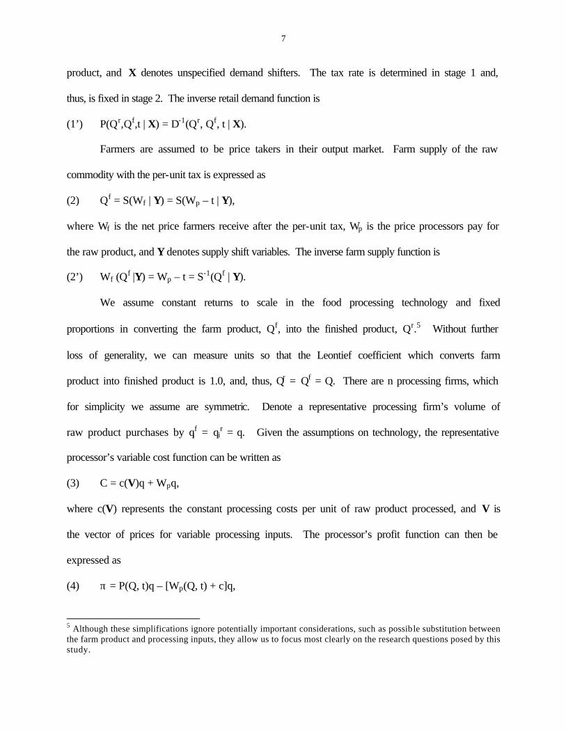
Farmers are assumed to be price takers in their output market. Farm supply of the raw

commodity with the per-unit tax is expressed as

(2) Qf = S(Wf | Y) = S(Wp – t | Y),

where Wf is the net price farmers receive after the per-unit tax, Wp is the price processors pay for

the raw product, and Y denotes supply shift variables. The inverse farm supply function is

(2’) Wf (Qf |Y) = Wp – t = S-1(Qf | Y).

We assume constant returns to scale in the food processing technology and fixed

proportions in converting the farm product, Qf, into the finished product, Qr.5 Without further

loss of generality, we can measure units so that the Leontief coefficient which converts farm

product into finished product is 1.0, and, thus, Qr = Qf = Q. There are n processing firms, which

for simplicity we assume are symmetric. Denote a representative processing firm’s volume of

raw product purchases by qif = qi

r = q. Given the assumptions on technology, the representative

processor’s variable cost function can be written as

(3) C = c(V)q + Wpq,

where c(V) represents the constant processing costs per unit of raw product processed, and V is

the vector of prices for variable processing inputs. The processor’s profit function can then be

expressed as

(4) π = P(Q, t)q – [Wp(Q, t) + c]q,

5 Although these simplifications ignore potentially important considerations, such as possible substitution between the farm product and processing inputs, they allow us to focus most clearly on the research questions posed by this study.

8

where Q = nq. The notation for the exogenous variables X, Y, and V is henceforth suppressed.

The first order condition to maximize (4) with respect to output choice, q, can be expressed as

r f

ff

d dP(Q,t) Q dW (Q) QP(Q,t) q [W (Q) t c] q 0

dq dQ q dQ q

π ∂ ∂= + − + + − =∂ ∂

.

This equation can be rewritten as

(5) ctdQ

)Q(dWQ)Q(W

dQ

)t,Q(dPQ)t,Q(P f

f ++θ+=ξ+ ,

or in elasticity form as:

(5’) fP(Q,t) 1 W (Q) 1 t c(Q,t) (Q)

ξ θ− = + + + Η ε ,

where dQ P

(Q,t)dP Q

Η = − is the absolute value of the total price elasticity of retail demand and is

a function of Q and t, and f

f

dQ W(Q)

dW Qε = is the price elasticity of farm supply and is a function

of Q. The parameters f f

f f

Q q

q Q

∂θ =∂

and r r

r r

Q q

q Q

∂ξ =∂

are the so-called conjectural elasticities. 2 ,

[0,1] depicts the degree of competition among processors in procuring the farm product, with 2 =

0 denoting perfect competition, 2 = 1 denoting pure monopsony (e.g., either a single buyer or

collusion among multiple buyers), and intermediate values of 2 denoting various magnitudes of

oligopsony power. In general, larger values of 2 denote greater departures from competition in

the procurement of the farm product. > , [0,1] measures departures from competition in the sale

of the finished product, with > = 0 denoting perfect competition, > = 1 denoting monopoly or

perfect collusion, and intermediate values of > representing various degrees of oligopoly power.

From (5’), the effect of imperfect competition on market behavior is determined jointly by the

market power index and the elasticity of supply or demand in the relevant market. For example,

9

the impact of a given level, >, of oligopoly power is greater the more inelastic the market

demand.

Equation (5’) involves the total price elasticity of demand because a change in market

quantity due to a change in price will induce a change in advertising expenditures, given a

constant check-off rate t. Based on the market demand function (1), this change in advertising

will induce a further change in demand. Imperfectly competitive firms who perceive that their

actions affect the market must take account of both the direct and indirect effect of price on

quantity (or, equivalently, quantity on price). Totally differentiating the demand function (1)

with respect to P yields

dP

dQ

A

Dt

P

D

dP

dQ

Q

A

A

D

P

D

dP

dQ

∂∂+

∂∂=

∂∂

∂∂+

∂∂= .

Note that A = tQ and, therefore, that ∂A/∂Q = t. Thus we have

ADt1

PD

dP

dQ

∂∂−

∂∂

= ,

or in elasticity form:

(6) p

A

dQ P

dP Q 1

ηΗ = =

− η,

where Q

P

P

DP ∂

∂−=η is the partial price elasticity of demand expressed in absolute value, and

Q

A

A

DA ∂

∂=η is the elasticity of demand with respect to advertising expenditure. Equation (6)

reveals that the total elasticity is greater in absolute value than the partial elasticity due to the

effect of quantity on advertising. For example, an increase in price reduces sales both due to

movement along the ceteris paribus demand curve and to a leftward shift in the demand curve

caused by lower advertising expenditures from the check-off program.

10

Given homogeneity among processors, equation (5’) represents an industry equilibrium

condition. It can be solved in conjunction with the consumer demand and farm supply functions

in (1’) and (2’), respectively, to obtain equilibrium values for Qf = Qr = Q, Wf = Wp – t, and P.

Equilibrium values are denoted by an asterisk and are functions of θ, ξ, t, c, the parameters

defining the supply and demand equations, and the exogenous variables X, Y, and V.

Any impacts on market prices and quantities from an exogenous shock can be examined

by totally differentiating (1), (2), and (5’) with respect to that factor. Thus, the following system

of equations describes the effect of a small change in the per-unit tax rate t:

(7) * * * * *

*dQ D dP D dA D dP D dQQ t

dt P dt A dt P dt A dt

∂ ∂ ∂ ∂= + = + + ∂ ∂ ∂ ∂

,

(8) * *

f

f

dQ S dW

dt W dt

∂=∂

,

(9) * * * *

f f2 2

dP P d dW W d1 1 1

dt dt dt dt

ξ ξ Η θ θ ε − + = + − + Η Η ε ε .

The system of equations can be rewritten in matrix form as follows:

(10)

*

*

*

f * ** ff H,t ,t

dQD D1 t 0 D

QdtA PA

S dP1 0 0

W dtP W

dW 1 E E0 1 (1 ) tH t

dtHε

∂ ∂ − − ∂ ∂ ∂ ∂ ∂ − = ∂ ξ θ − − ξ θ − − + ε ε

,

where H,t

d tE

dt

Η=Η

measures the percentage change in / due to a one percent increase in the

per-unit tax, and E,, t =d t

dt

εε

is the percentage change in , due to a one percent increase in t. Thus

the effect of a small change in t on market prices and quantity can be determined from equation

(10) as follows:

11

(10’)

* *** f

,t ,tf

* * ** f

,t ,t *f

* * *f * f

,t ,t

S D P W DdQ [(1 )Q (1 E ]E )W A t t Pdt

dP 1 D P W D S(1 )Q (1 E E )(1 t )

dt A t t A W

dW D P W D(1 )Q (1 E E )

dt A t t P

Η ε

Η ε

Η ε

∂ ξ ∂ ξ θ ∂ − + − − ∂ Η ∂ Η ε ∂ θ ∂ ξ θ ∂ ∂ = + + − − − λ ε ∂ Η ε ∂ ∂ ξ ∂ ξ θ ∂ − − − − Η ∂ Η ε ∂

,

where f

D S D(1 )(1 t ) (1 )

A W P

ξ ∂ ∂ θ ∂λ = − − − +Η ∂ ∂ ε ∂

.

Stage 1 Solution:

In stage 1, the marketing board selects the per-unit tax rate t and corresponding advertising

expenditure to maximize producers’ surplus (PS):

(11)

* *f

f

W (Q ( t ) )

f fW ( 0 )

max PS S(W )dW ,

t

= ∫

where Wf(0) is the supply curve intercept. The first-order condition to maximize equation (11) is

(12) 0t

Q

Q

W))t(W(S

t

)t(W))t(W(S

t

PS *

*

*f*

f

*f*

f =∂

∂∂∂

⋅=∂

∂⋅=

∂∂

.

From equation (12) we obtain

(13) 0t

Q*

=∂

∂,

as the condition characterizing the optimal tax rate. Equation (13) indicates that the optimal per-

unit tax rate is reached when the supply-reducing effect of a higher tax rate is just balanced by

the demand-expanding effect of the advertising expenditures funded by the tax, so that a change

in the tax rate has no effect on equilibrium quantity. This same condition was derived by ACC

in their study of check-off-funded advertising under perfect competition.

12

Substituting this optimality condition into the comparative statics matrix (10’) in place of

dQ/dt, we obtain

(14) *

*H,t

D P D1 Q (1 E )

A t P

ξ ∂ ξ ∂ − = − Η ∂ Η ∂ .

Rearranging (14) and writing it in elasticity form yields

(15) *

A** *

P,t

A (1 /H)PP Q

(1 E )t Η

η − ξ=ξη −Η

.

Finally, using the fact that P

t

PQ

tQ

PQ

A == , equation (15) can be rewritten as

(15’)

*A A A

,t ,t* *P P P

A1 E E

P Q Η Η

η ξ ξ η ξ η = − + = + − η Η Η η Η η .

All elasticities are evaluated at the imperfectly competitive equilibrium.

Equation (15’) indicates that the optimal ratio of check-off-funded advertising

expenditures to total sales revenue is equal to the ratio of the partial elasticities of demand with

respect to advertising and to price, i.e., the condition from Dorfman and Steiner and ACC, and an

additional term. This term consists of the oligopoly distortion term, >//, times the difference

between H,tE and 0A/0P. H,tE measures how the total price elasticity of demand changes in

response to a small increase in t.

Using (6), we can express d//dt as follows:

(16) P A P A2

A

dH (d /dt)(1 ) (d /dt)

dt (1 )

η −η + η η=− η

.

In general, (16) cannot be signed. However, under plausible conditions d//dt > 0, so that

increasing t and, correspondingly, A makes demand more elastic in total, thereby reducing the

oligopoly distortion and providing an additional benefit to farmers from check-off funded

advertising. Two effects are at work in determining d0P/dt. First, the supply shift induced by )t

13

> 0 causes a movement upward along the existing demand curve. For most functional forms,

demand is more elastic at higher prices. Second, successful advertising shifts demand. For

example, if advertising induces a parallel shift in demand, as is often assumed in empirical

studies, this effect also makes demand more elastic. The benefit to reducing the oligopoly

distortion is proportional to the magnitude of the distortion as (15’) indicates. However, an oft-

cited rationale for advertising is to make demand for the advertised product less elastic, in which

case producer-sponsored advertising has the perverse effect of increasing the oligopoly distortion

ceteris paribus and creating a disincentive for producer advertising.

If d//dt = 0, then the condition for optimal advertising intensity collapses to

* *A

* * *P

A t1 ,

P Q P

η ξ = = − η Η

i.e., the 0A/0P ratio characterizing optimal advertising intensity in the DS and ACC formulations

is reduced by a factor determined by the oligopoly distortion. An oligopoly processing sector

will always capture some of the benefits from an advertising-induced demand shift, whereas a

competitive processing sector captures none, given a constant returns processing technology.

However, the oligopoly processors also bear some of the incidence of the tax, whereas

competitive processors bear none of it. Although it is possible that the optimal tax rate is higher

in the presence of oligopoly power in the marketing sector, (15’) shows that the advertising

intensity for a farm commodity board is always less unless the advertising represents a way to

reduce the oligopoly distortion.

Importantly, oligopsony power per se has no effect on the optimal A/S ratio. Because the

supply elasticity itself has no effect on the optimal A/S ratio, as revealed by ACC’s extension of

the DS condition to check-off funded advertising, neither does the exploitation of the supply

curve by an oligopsonist. However, this result simply means that optimal check-off funded

14

advertising in a market with only oligopsony power is characterized by the same DS condition as

applies in a perfectly competitive industry. It does not mean that the actual optimal advertising

intensities are the same. In particular, oligopsony power causes lower sales and higher prices

relative to competition, meaning that 0P is evaluated at a point on the demand curve to the left of

the competitive equilibrium. Most demand functions are relatively more elastic at an imperfect

competition equilibrium, causing the optimal advertising intensity to be less, ceteris paribus,

than under perfect competition.

Comparison to Optimal Advertising Financed by a Lump-Sum Tax

Our greatest interest is in advertising generated from a check-off program because of its

application in the real world. However, it is also instructive to analyze the optimality conditions

under imperfect competition for commodity advertising that is generated from a lump-sum tax,

i.e., the case analyzed by NW for perfect competition. The optimality condition is set forth

below, with its derivation relegated to the appendix:

(17) P,A

*A P

* * *P p P

EA 1 ( / )

P Q / f 1 ( / ) (1 ( / ))P (1 ( / ))Wηξη − ξ η

= +η + ε + θ ε − ξ η ε + + θ ε η

.

Where f* = W*/P* is the farm revenue share in equilibrium, P

P,A

P

d AE

dAη

η=η

, and all other terms

are as defined previously.

When the market is competitive (i.e., θ = ξ = 0) and the constant marginal processing cost

is zero (i.e., f* = 1 and P* = W*), the expression in (17) reduces to the NW condition.6

6 Nerlove and Waugh’s formulation does not incorporate a marketing sector, so marketing costs are implicitly zero. Incorporating a constant cost competitive marketing sector into NW’s model and assuming fixed proportions between the farm product and retail product, results in the following relationship between elasticity of supply at retail, ,r and elasticity of farm supply, ,: ,r = ,/f. Thus, the NW formulation generalizes immediately to accommodate this type of marketing sector simply by interpreting their supply elasticity as the retail supply elasticity.

15

Comparing (15’) and (17), we see that both the oligopoly and oligopsony power distortions (>/0P

and 2/,, respectively) reduce the optimal advertising-to-sales ratio when advertising funds are

generated by a lump-sum tax. Under a lump-sum tax on producers, processors with oligopoly

and/or oligopsony power capture some of the advertising benefits without bearing any of the

costs.

The second term in (17) reflects that advertising might affect the elasticity of demand

and, therefore, influence the oligopoly distortion. As in the case of a per-unit tax, if advertising

makes demand more elastic, the opportunity to reduce the oligopoly distortion represents an

additional incentive for producers to undertake advertising. The opposite is true if advertising

acts to make demand less elastic.7

Linear Model Formulation

We turn now to a linear formulation of the model developed in the preceding section. The linear

model is used to conduct simulation analyses of the impact of processor market power on the

magnitude of optimal advertising and the distribution of advertising benefits and to analyze the

possible impact of market power on optimal commodity advertising in the U.S. beef and dairy

industries.

The total market demand is:

(18) Q = a – αP,

And the inverse farm product supply is

(19) Wf = b + βQ.

7 Note that for the lump -sum tax, use of the partial demand elasticity is correct because there is no direct feedback between output and the advertising expenditure.

16

To facilitate the subsequent simulation analysis, we solve first for the competitive market

equilibrium (superscript c) in the absence of any advertising (subscript o). Through choice of

units of measurement, the competitive equilibrium price and output are normalized to

be c co o(P ,Q ) (1,1)= . All subsequent solutions can then be evaluated relative to the competitive

equilibrium without advertising.

(20) c c c0 0 f 0

a b c a (b c)P 1, Q 1, and W 1 c

1 1

β + + −α += = = = = −βα+ β α +

,

where c is the per-unit processing cost. The relations among the parameters are thus: a = 1 + α,

b = 1 – c – β = fc – β , where fc = 1 – c denotes the farm share of total industry revenue under

perfect competition. In addition, the demand and supply slope parameters, " and $, can be

expressed in terms of the retail price elasticity of demand and farm price elasticity of supply,

both evaluated at the competitive equilibrium:8

c c cc co oP c c c

o o

P WQ Q 1 f, (1 c) .

P Q W Q

∂ ∂η = = α ε = = − ⇒ β =∂ ∂ β ε

Employing these normalizations and following the same approach as set forth in the general

model, the equilibrium in the absence of advertising (subscript 0) in the oligopoly-oligopsony

model is denoted by an asterisk and is characterized as follows:

(21) *c c c

* * * *0P0 0 f 0 0c

P

a Q1 (f / )Q , P , W b Q

−+ η ε= = = + βΩ η

,

8 In the linear model, the values of both 0P and , depend in general upon the point of evaluation. However, their values at any one point, say the competitive equilibrium, will condition their values at all other points. Thus, we express both 0P and , in terms of their values at the competitive equilibrium.

17

where Ω = (1 + ξ) + (1 + θ)αβ = (1 + ξ) + (1 + θ)fc cPη /εc. S measures the cumulative distortion

due to oligopoly and oligopsony power in the linear model. If 2 = > = 0, the equilibria in (20)

and (21) are identical.

Now consider the introduction of commodity advertising funded by a per-unit tax, t, on

producers. Advertising is assumed to induce a parallel shift in retail demand as follows:9

(18’) Q = a + z(A) – αP,

where A = tQ. To facilitate obtaining an interior optimum for A in the simulation modeling, we

need to establish a specific functional relationship for z(A) that insures a positive and concave

demand response to advertising, i.e., zN(A) > 0, zNN(A) < 0 . The square root formulation,

z(A) A tQ= γ = γ ,

was chosen both because of its simplicity and its ability to fit the data well in several empirical

studies of demand response to advertising (e.g., Alston et al. (1997, 1998) and Gasmi, Laffont,

and Vuong). The parameter ( represents the effectiveness of advertising in shifting demand,

given the square root formulation.

It is straightforward to apply the framework of the general model to the linear version set

forth in this section and solve for the stage 2 equilibrium.10 Consider the equilibrium condition

in (5). Differentiate the demand function in (18’) and supply function in (19) to obtain:

β=

−γ

α=

dQ

dWand1

Q2

t1dQdP f .

Substitute these expressions into (5), convert to elasticities, and solve for Q to obtain:

9 This assumption is consistent with most empirical research on advertising impacts and also simplifies the simulation modeling. However, it does entail a cost in generality because an advertising-induced parallel demand shift in the linear model insures that demand is more elastic at the new equilibrium. 10 There is no need to solve separately for the competitive equilibrium with commodity advertising because the imperfect competition model nests the competitive outcome as a special case, namely when both 2 and > are zero.

18

(22)

22 2 c c c c

P P* (2 ) t (2 ) t 16 (1 f / t)Q

4

+ ξ γ + + ξ γ + Ω + η ε − η =

Ω ,

Solutions for P* and Wf* follow immediately. Recall that the optimal per-unit tax rate, t*, is

characterized by the condition dQ*/dt = 0. Thus, differentiating (22) with respect to t and setting

the expression to zero, we obtain

(23) c c c 2 2

* Pc c 2 2P P

(1 f / )(2 )t

[16 (2 ) ]

+ η ε + ξ γ=η Ωη − + ξ γ

.

The optimal advertising expenditure, A* = t*Q* is obtained by combining (22) and (23).

The optimal tax rate in the linear model is characterized by six parameters: the farm share

(fc), the price elasticity of supply of the farm product (,c), the price elasticity of demand at retail

( cPη ) (all evaluated at the competitive equilibrium without advertising), the degree of oligopoly

power (>), the degree of oligopsony power (2), and the effectiveness of advertising (γ). Key

comparative static results for the linear model are as follows:

* * * * * * *

c cP

t A t t t A t(24) 0, 0, 0, 0, 0, 0, and 0

∂ ∂ ∂ ∂ ∂ ∂ ∂> >=< < >=< < < >∂ξ ∂ξ ∂η ∂ε ∂θ ∂θ ∂γ

.

Increases in oligopsony power cause a decrease in the optimal tax rate and the industry output.

Since A* = t*Q*, both effects contribute to reducing the optimal amount of advertising

expenditures. An increase in the degree of oligopoly power, however, causes producers’ optimal

tax rate to increase because in the linear model both the tax rate and the advertising expenditure

it generates work to make demand more elastic. However, because the output base to which the

tax rate is applied decreases as a function of >, the net effect of > on A* is ambiguous.

Among the other market parameters, * cPt /∂ ∂η < 0, reflecting that it is unambiguously

better to shift via advertising a demand curve that is inelastic rather than elastic, and this basic

result is unaffected by the degree of competition in the market. However, the sign of Mt*/M,c is

19

ambiguous. Under perfect competition, Mt*/M,c < 0 because an elastic supply response converts

an advertising-induced demand shift primarily into an output increase rather than a price

increase. However, as noted, oligopsony power reduces the optimal tax rate, and the effect of

oligopsony power is exacerbated by an inelastic producer supply, thus offsetting the

aforementioned tendency for inelastic supply to induce a higher tax rate. Finally, t* and A* are

both increasing as a function of the advertising effectiveness parameter, (.

Producers’ benefit from advertising is measured by the change in their producer surplus

in the equilibrium with advertising relative to the equilibrium without advertising:

(25) c

* 2 * 21 0c

fPS [(Q ) (Q ) ]

2∆ = −

ε.

Similarly, processors’ benefit may be measured by the change in their profits across the two

scenarios: * *1 0 .∆ π = π − π

Simulation Model Simulations can enhance our understanding of the impact of imperfect competition on the level

of commodity advertising and the distribution of benefits and costs from advertising for

alternative sets of plausible values for the market parameters. After normalization, the linear

model is characterized by six parameters (f, ,, 0P, 2, >, and (). The key parameters for purposes

of the simulation are those characterizing the extent of oligopoly and oligopsony power in the

market, > and 2, respectively. Thus, we wish to examine optimal commodity advertising for

alternative values of > and 2, given a set of plausible base values for the other parameters. In all

cases, the farm share under perfect competition was fixed at one half: fc = 0.5.11 For the base

11 This value is roughly in line with farm share for meats, eggs, and dairy products.

20

simulation, we also set c cp 1.0η = ε = , i.e., the price elasticities of demand and supply are unitary

at the competitive equilibrium.12

The advertising effectiveness parameter, (, was fixed based upon its relation to ηA, the

advertising elasticity of demand. Given the retail demand function in (18’) and the square-root

formulation for demand response to advertising, 0A, evaluated at the competitive market

optimum for A and equilibrium for Q, can be expressed as follows:

(27)c cc c

1A c c c

1 1 1

t QA t.

2Q 2Q 2 Q

γγ γη = = =

c1Q and tc can be expressed using (22) and (23), respectively, and the entire expression in (27)

can be solved to yield P A( , , , f )γ = γ η η ε , i.e., ( can be expressed in terms of the other market

parameters and 0A, the advertising elasticity of retail demand. Estimates of 0A are available for

various commodities from previous empirical studies.13 Based on a review of these studies, we

chose 0A = 0.05 as a representative value for the base simulation.

Simulation results

Figure 1 illustrates the impact of imperfect competition on the optimal level of taxation, t*, for

the base simulation. The optimal tax is $0.052 under perfect competition (5.2% given Pc = 1).

12 We also experimented with other choices of parameterizations for c

Pη and ,c. From the comparative statics

expressions in (24), we know that increasing cPη ceteris paribus reduces the optimal investment in advertising. For

example, given 2 = > = 0.5, an increase in the demand elasticity (evaluated at the competitive equilibrium) from 0.6 to 2.0 causes the optimal advertising expenditure to fall by 80%. Although, in general, the effect of ,c on t* and A* is ambiguous, in this simulation increasing ,c on the interval [1, 3.0] caused the optimal expenditure on advertising to increase, ceteris paribus, when 2 = > = 0.5. Even though the increase in the producer price generated by a given demand shift is decreasing in ,, a more elastic supply reduces the extent of oligopsony exploitation for a given level of 2, and this latter effect is dominant when oligopsony power is important, as is true when 2 = 0.5. 13 See Forker and Ward and Ferrero et al. for summaries of this work.

21

Consistent with the comparative statics results, t* decreases as a function of the oligopsony

power exercised in the market, falling ultimately to $0.038 for the case of pure monopsony. The

tax is increasing in the level of oligopoly power, rising from $0.052 to $0.071 as > increases from

0 to 1. Joint oligopoly-oligopsony power, thus, induces offsetting effects on t*. Oligopoly, in

general, is more important than oligopsony because the latter affects only the farm product

segment of the input market (fc = 0.5), and, thus, t* is increasing as a function of the degree of

joint oligopoly/oligopsony power.

Although oligopoly and joint oligopoly/oligopsony generate a higher level of per-unit

taxation than does perfect competition, the amount of advertising funds expended, A* = t*Q*, is

decreasing as a function of the magnitude of market power for all equilibria in the simulation, as

Figure 2 illustrates. The decrease in Q* due to market power dominates the increase, if any, in t*.

Figure 3 lends further perspective by depicting the optimal A/S ratio as a function of processor

market power. The optimal A/S ratio declines as a function of the degree of oligopsony power

and joint oligopoly/oligopsony power. However, oligopoly power has little effect on the A/S =

t/P ratio. Both t* and P* are higher due to oligopoly power, and their effects roughly offset.

Referring again to the general condition in (15’) governing the optimal A/S ratio, EH,t is

necessarily positive in the linear model with a parallel demand shift and also greater than the

ratio 0A/0P. Thus, advertising makes demand more elastic, reducing the oligopoly distortion and

providing an additional incentive for producers to advertise in oligopolistic markets.

The impact of market power on the magnitude and distribution of benefits is more

pronounced than its effect on advertising expenditures. We examine benefits accruing to

producers and to processor/retailers only. Although consumers clearly bear a portion of the

burden of an advertising tax in the form of higher prices, it is much less clear whether and how

22

they benefit from advertising.14 Total benefits accruing jointly to producers and processors from

the optimal expenditure on advertising (the sum of the change in producer surplus and processor

profits) for alternative market power configurations are depicted in Figure 4. The percentage of

the total benefits going to producers is provided in Figure 5.

Although processor oligopsony power reduces the optimal advertising expenditure

relative to perfect competition, the total benefits generated from the amount that is spent increase

over a range of values for 2. Although producers’ benefits are strictly decreasing as a function

of 2, processors’ benefits are increasing in 2. Oligopsony power enables processors to convert a

given advertising-induced demand shift into a relatively greater impact on price than would

occur under perfect competition, thereby causing total benefits to rise over a range of values for

2. For the highest levels of oligopsony power (2 $ 0.81), the reduction in advertising

expenditure caused by market power dominates the enhanced ability to extract profits from the

amount that is spent, and total benefits to producers and processors decline.

The output restriction that is beneficial to processors is harmful to producers. Producers’

benefits from advertising decline monotonically as a function of 2. For example, for 2 = 0.2,

producer benefits are 18% less than at the competitive optimum and 38% less for 2 = 0.5. From

Figure 5, processors capture 50% of the total benefits when 2 = 0.5 and over half of the benefits

for all 2 > 0.5.

Under oligopoly power, total benefits to producers and processors from advertising are

always less in the base simulation than under perfect competition.15 This result may seem

14 For example, is it appropriate to attribute benefits to consumers from an advertising-induced shift in consumer demand? These issues are well beyond the scope of this paper. See Alston, Chalfant, and Piggot for a recent discussion of this issue. 15 This result does not hold in general because plausible base values for c

P candη ε can be found wherein total

benefits are increasing over a range of values for >.

23

paradoxical because advertising expenditures for a given value of > are always greater than for a

comparable value of 2. The reason is the effect of advertising on the elasticity of demand.

Given the linear model formulation, both the supply shift induced by t* > 0 and the parallel

demand shift induced by A* > 0 cause demand to be more elastic at the equilibrium, ceteris

paribus. As a result, processors’ ability to exploit a given level of oligopoly power is

diminished. This effect applies not just to the incremental demand created by the advertising but

to the demand in total. Both farmers and consumers benefit from this reduction in the oligopoly

distortion. As Figure 5 shows, processors’ percentage of the advertising benefits under oligopoly

(i.e., 100% minus producers’ percentage) is always less than their share under comparable

oligopsony and is only 37% (100% minus farmers’ 63% share) at its maximum when > = 1 (i.e.,

pure monopoly).

When both oligopoly and oligopsony power are present in a market, the effect on

producers’ benefits from commodity advertising can be extreme. For example, even modest

market power as manifest by > = 2 = 0.2 reduces producers’ advertising benefits by 30% relative

to competition. More extreme market power as represented by > = 2 = 0.5 reduces producers

benefits by 54%.

As a final comparison, we show how imperfect competition distorts the impact from a

given advertising expenditure. Specifically, we took the optimal level of advertising expenditure

from each of the imperfectly competitive scenarios under consideration and asked how the

magnitude and distribution of impacts would have differed had that same amount been generated

and expended under conditions of perfect competition. There are two major impacts. First,

because imperfect competition reduces total production and sales, a given advertising

expenditure is generated with a lower tax rate when the market is competitive. Second,

24

imperfectly competitive processors incur a share of the tax burden and receive a share of the

advertising benefits.

Figure 6a reports the percentage reduction in producer benefits from expending the

amounts of advertising money shown in Figure 2 under conditions of imperfect competition

rather than perfect competition. Producer benefits from an advertising expenditure are always

lower if the marketing sector is imperfectly competitive. The reduction in producer benefits

ranges from 9% when (>, 2) = (0.1, 0) to 70% for the extreme case when (>, 2) = (1, 1).

However, the benefit accruing jointly to producers and marketers from a given advertising

expenditure can be higher under imperfect competition, as Figure 6b illustrates. For the market

parameters studied in our simulation, a given expenditure always results in greater total benefits

under oligopsony power than perfect competition because oligopsony power converts the

demand shift proportionately more into a price effect than an output effect. However, oligopoly

power always reduces the joint producer-marketer benefits relative to competition in the base

simulation. Although oligopoly power also enables a demand shift to be converted into a higher

consumer price than is attainable under perfect competition, this effect is more than offset by the

reduction in the oligopoly distortion caused by the increase in the elasticity of demand. Joint

oligopoly/oligopsony power thus provides an intermediate case, with greater total benefits than

perfect competition for modest levels of market power and less total benefits for more extreme

levels of oligopoly/oligopsony.

Application to U.S. Beef and Dairy Advertising

Here we present illustrative applications to U.S. industries that feature generic advertising

programs. Beef and Dairy were chosen because of their importance in the realm of commodity

25

advertising and because estimates of the necessary parameters are available from previous

studies. For beef, we utilized the following parameters: 2 = 0.178, > = 0.223, 0P = 0.527, , =

1.689, fc = 0.57, and 0A = 0.012.16 Based on the linear simulation model and the indicated

parameters, the optimal A/S ratio in the imperfectly competitive market structure is 0.017

compared to 0.023 if the market were competitive. Optimal advertising is reduced 16.5% by

imperfect competition in the processing sector. Producers’ benefits from advertising are reduced

by 31% from their magnitude under a hypothetical regime of perfect competition, and packers

capture 55% of the benefits generated from the optimal advertising expenditure.

The dairy application relied on the following parameters: 2 = 0.0, > = 0.18 (Liu, Sun, and

Kaiser), 0P = 0.16 (Suzuki and Kaiser), , = 0.14, fc = 0.45, and 0A = 0.035 (Kaiser et al.).17 For

these parameters, the optimal A/S ratio under a hypothetical competitive regime is 0.017. Under

imperfect competition, it is 0.011. However, total advertising expenditure is only about 5%

lower due to imperfect competition, and producer benefits are reduced by only 15%. Suppose,

however, that > = 2 = 0.18 and all other parameters are as before (see footnote 17). Then the

optimal A/S ratio is only 0.009, roughly half its value under competition, optimal advertising

expenditures are 15% lower than under competition, and producers’ benefits from advertising are

reduced by 28%.

16 The market power parameters for the beef industry, 2 and >, are from Azzam and Pagoulatos, the demand and supply elasticities are from Azzam and Schroeter, and the advertising elasticity of demand is derived from Ward and Lambert. There is controversy regarding both the extent and importance of market power in the U.S. beef sector and the effectiveness of generic beef advertising, so the estimates utilized here should be considered as illustrative and not definitive. See Sexton and Lavoie regarding the market power controversy and Coulibaly and Brorsen on disagreements over the effectiveness of beef promotions. 17 The oligopsony power parameter was set at zero to reflect that considerable dairy processing capacity is in the hands of producer-owned cooperatives. Oligopsony power could, however, be a concern if it existed at other stages of the marketing chain, e.g., retailing.

26

Conclusions

Much has been written about the rapid increases in concentration worldwide in food marketing.

The consequences of this consolidation for the exercise of market power continue to be debated.

This paper joins the growing list of studies that examine the implications of departures from

competition for various aspects of industry behavior. Prior work has emphasized the impacts

upon an industry of exogenous forces, such as research-induced supply shifts (Alston, Sexton,

and Zhang and Hamilton and Sundig) or various trade policy instruments (McCorriston and

Sheldon and Paarlberg and Lee). A unique feature of this study is to examine the impact of

imperfect competition on an endogenous industry policy instrument—the level of monies to

collect and expend on a commodity advertising program.

Results demonstrate that in the presence of imperfect competition, the optimal

advertising-to-sales (A/S) ratio for funds generated from a per-unit tax is not, in general,

characterized by the ubiquitous Dorfman-Steiner condition, shown to hold for the competitive

case by Alston, Carman, and Chalfant. Neither does the well-known Nerlove-Waugh

formulation for lump-sum funding hold under conditions of imperfect competition.

An imperfectly competitive marketing sector will capture a portion of the benefits from

commodity advertising, but it will also bear a share of the costs under funding by a per-unit tax

or check off. A possibly important benefit of generic advertising in the presence of

processor/retailer oligopoly power is that advertising may make demand more elastic, thereby

reducing the distortion from oligopoly power and increasing producer welfare—a benefit that is

not present under conditions of perfect competition.

Results from simulations based on a linear version of the general model showed that the

optimal check-off rate from producers’ perspective is actually increasing as a function of the

27

degree of oligopoly power in the market. In contrast the optimal tax rate is always lower under

oligopsony power or joint oligopoly/oligopsony power. In all cases evaluated in the simulation

model, producers’ benefits from advertising were lower, in some cases by half or more, in the

presence of processor market power than if the market were competitive.

Although the intent expressed in the various legislation that enables industries to conduct

generic advertising is that farm producers are to be the primary beneficiaries of the programs, our

analysis shows that an imperfectly competitive marketing sector may capture half or more of the

net benefits generated by the programs. Oligopsony power tends to have a larger, negative

impact on farmers’ benefits from advertising than oligopoly power because advertising may

reduce the oligopoly distortion through its effect on the demand elasticity. One implication of

this result is that in markets suspected of being oligopolistic, empirical studies of advertising

benefits should attempt to test not only whether advertising is shifting demand but also whether

it has made demand more or less elastic.

28

Appendix: Optimal Commodity advertising From a Lump-Sum Tax

Here we derive the condition characterizing optimal commodity taxation under imperfect

competition in the food-processing sector when the advertising funds are generated from a lump-

sum tax. The retail demand function for the finished product is represented by

(A1) Qr = D(P,A | X),

or in inverse form by

(A1’) P = D-1(Qr, A | X).

The inverse farm supply function is

(A2) W(Qf) = S-1(Qf | Y).

A representative processing firm’s volume of raw product purchases is denoted by qf. Given our

previous assumptions on the processing technology, the processor’s variable cost function can be

written as:

(A3) C = c(V)qf + Wqf,

and the processor’s profit function can then be expressed as

(A4) π = D-1(Qr, A)qr – [W(Qf,) + c]qf

where qr is the quantity of processed product produced. As before we let qf = qr = q, and

r f r fQ Q Q nq nq .= = = = The notation for the exogenous variables X, Y, and V is henceforth

suppressed. Maximizing profit with respect to q results in the following first-order condition:

(A5) ∂π/∂q = P + P’(Qr, A)(∂Qr/∂q)q – (W + c) – W’(Qf)(∂Qf/∂q)q = 0.

Equation (A5) can be written in elasticity form as

(A6) P

P(Q,A) 1 W(Q) 1 c ξ θ − = + + η ε

.

All notation is the same as in the main body of the paper.

29

From equations (A1), (A2) and (A6), we can solve for the equilibrium values of Qf = Qr,

P, and W as functions of θ, ξ, A, c, the parameters defining the supply and demand equations,

and the exogenous variables X, Y, and V. As in the main text, equilibrium values are indicated

by an asterisk. With a lump-sum tax, there is no feedback effect from quantity to advertising

expenditure, and, thus, the total price elasticity of demand is simply the partial elasticity, 0P.

However, it should be recognized that in general 0P is a function of both Q and A, and , is a

function of Q.

The effect of an exogenous change in A can be adduced by differentiating (A1), (A2),

and (A6) with respect to A:

(A7) dQ D dP D

dA P dA A

∂ ∂= +∂ ∂

,

(A8) dQ S dW

dA W dA

∂=∂

,

(A9) P2 2

P P f

dP P d dW W d1 1

dA dA dA dA

ξ ξ η θ θ ε− + = + + η η ε ε

.

The system of equations can be rewritten in matrix form:

(A10)

P ,A ,A

PP f

D dQ1 0 D

P dAA

S dP1 0 0

W dAP W

dW E E0 1 (1 ) A A

dAη ε

∂ − ∂ ∂ ∂ ∂ − = ∂ ξ θ ξ θ − − − − + η ε η ε

,

where P,A

P

P

d AE

dAη

η=η

, and ,A

d AE

dAε

ε=ε

are, respectively, the percentage change in the price

elasticity of demand and price elasticity of supply due to a 1 percent increase in A. Thus the

effect of a small change in A on market prices and quantity can be determined by simultaneously

solving the equation system (A10):

30

(A10’)

P

P

P

*

,A ,A

P P

*

,A ,A

f P*

,A ,AP P

S D P W DdQ [(1 )( E E )W A A A PdA

dP 1 D P W S(1 ) E E

dA A A A WdW D P W D

(1 ) ( E E )dA A A A P

η ε

η ε

η ε

∂ ξ ∂ ξ θ ∂ − − − ∂ η ∂ η ε ∂ θ ∂ ξ θ ∂ = + − + ψ ε ∂ η ε ∂ ξ ∂ ξ θ ∂− + + η ∂ η ε ∂

,

where T f

S D(1 ) (1 )

W P

ξ ∂ θ ∂ψ = − − +η ∂ ε ∂

.

Stage 1 Solution

In stage 1, the marketing board chooses A to maximize producers’ net surplus:

(A11) ∫ −=− ))A(Q(W)0(W

**AdW)W(SAPS ,

where W(0) is the supply curve intercept. The first-order condition for maximizing equation

(A11) is

(A12) 01A

Q

Q

WQ1

A

)A(W))A(W(S

A

)APS( **

** =−

∂∂

∂∂=−

∂∂

⋅=∂

−∂.

Producers bear the entire burden of a lump-sum tax. Thus, equation (A12) is simply a condition

that the marginal revenue to producers from a marginal increase in advertising expenditure just

equal the marginal cost of the expenditure. From equation (A12) we obtain

(A13)* *

*

Q

A W

∂ ε=∂

.

Imposing this optimality condition for dQ*/dA in (A10’), we obtain

(A14) P,A

*

* *P P

D P D1 E

A A P Qη

ξ ∂ ξ ∂ ψ− − = η ∂ η ∂

.

Rearranging (A14) equation and writing it in elasticity form results in the following expression

for the optimal advertising-to-sales ratio when advertising is funded by a lump-sum tax:

P,A

*A P

* * *P p P

EA 1 ( / )

P Q / f 1 ( / ) (1 ( / ))P (1 ( / ))Wηξη − ξ η

= +η + ε + θ ε − ξ η ε + + θ ε η

.

31

Figure 1: The Impact of Imperfect Competition on the Optimal Advertising Tax Rate

Figure 2: The Impact of Imperfect Competition on the Optimal Advertising Expenditure

Figure 3: Optimal Advertising-to-Sales Ratio under Imperfect Competition

0 . 0 0 . 1 0 . 2 0 . 3 0 . 4 0 . 5 0 . 6 0 . 7 0 . 8 0 . 9 1 . 0

m a r k e t p o w e r i n d e x

0 . 0 4

0 . 0 4 5

0 . 0 5

0 . 0 5 5

0 . 0 6

0 . 0 6 5

0 . 0 7

t*

o l i g o p s o n y o l i g o p o l y b o t h

0 . 0 0 . 1 0 . 2 0 . 3 0 . 4 0 . 5 0 . 6 0 . 7 0 . 8 0 . 9 1 . 0

m a r k e t p o w e r i n d e x

0 . 0 3

0 . 0 3 5

0 . 0 4

0 . 0 4 5

0 . 0 5

0 . 0 5 5

A *

o l i g o p s o n y o l i g o p o l y b o t h

0 . 0 0 . 1 0 . 2 0 . 3 0 . 4 0 . 5 0 . 6 0 . 7 0 . 8 0 . 9 1 . 0

m a r k e t p o w e r i n d e x

0 . 0 3

0 . 0 3 5

0 . 0 4

0 . 0 4 5

0 . 0 5

A * /S *

o l i g o p s o n y o l i g o p o l y b o t h

32

Figure 4: Total Benefit to Producers and Processors from Advertising

∆PS+∆Π

Figure 5: Producers’ Shares of the Total Advertising Benefit under Imperfect Competition

0 . 0 0 . 1 0 . 2 0 . 3 0 . 4 0 . 5 0 . 6 0 . 7 0 . 8 0 . 9 1 . 0

m a r k e t p o w e r i n d e x

0 . 0 1 2

0 . 0 1 4

0 . 0 1 6

0 . 0 1 8

0 . 0 2

0 . 0 2 2

0 . 0 2 4

o l i g o p s o n y o l i g o p o l y b o t h

0.0 0.1 0.2 0.3 0.4 0.5 0.6 0.7 0.8 0.9 1.0

m a r k e t p o w e r i n d e x

3 0

4 0

5 0

6 0

7 0

8 0

9 0

1 0 0

%

o l i g o p s o n y oligopoly b o t h

33

Figure 6a: Change in Producer Benefits from Advertising Due to Imperfect Competition

Figure 6b: Change in Total Benefits from Advertising Due to Imperfect Competition

0 . 0 0 . 1 0 . 2 0 . 3 0 . 4 0 . 5 0 . 6 0 . 7 0 . 8 0 . 9 1 . 0

m a r k e t p o w e r i n d e x

- 7 0

- 6 0

- 5 0

- 4 0

- 3 0

- 2 0

- 1 0

0

%

o l i g o p s o n y o l i g o p o l y b o t h

0 . 0 0 . 1 0 . 2 0 . 3 0 . 4 0 . 5 0 . 6 0 . 7 0 . 8 0 . 9 1 . 0

m a r k e t p o w e r i n d e x

- 2 0

- 1 0

0

1 0

2 0

3 0

4 0

%

o l i g o p s o n y o l i g o p o l y b o t h

34

References

Alston, J.M., H. F. Carman, and J.A. Chalfant. “Evaluating Primary Product Promotion: The

Returns to Generic Advertising by a Producer Cooperative in a Small, Open Economy.” In E.W. Goddard and D.S. Taylor eds., Promotion in the Marketing Mix: What Works, Where, and Why, Toronto, University of Guelph.

Alston, J.M., J.A. Chalfant, and N.E. Piggot. “The Incidence of the Costs and Benefits of

Generic Advertising.” American Journal of Agricultural Economics 82(2000): in press. Alston, J.M., J.W. Freebairn, and J.S. James. “Beggar-thy-Neighbor Advertising: Theory and

Application to Generic Commodity Promotion Programs,” Working Paper, University of California, Davis, 2000.

Alston, J.M., R.J. Sexton, and M. Zhang. “The Effects of Imperfect Competition on the Size and

Distribution of Research Benefits.” American Journal of Agricultural Economics 79(1997): 1252-1265.

Alston, J.M., J.A. Chalfant, J.E. Christian, E. Meng, and N.E. Piggot. “The California Table

Grape Commission’s Promotion Program: An Evaluation.” Giannini Foundation Monograph No. 43, University of California, Division of Agriculture and Natural Resources, 1997.

Alston, J.M., H.F. Carman, J.A. Chalfant, J.M. Crespi, R.J. Sexton, and R.J. Venner. “The

California Prune Board’s Promotion Program: An Evaluation.” Giannini Foundation Research Report No. 344, University of California, Division of Agriculture and Natural Resources, 1998.

Azzam, A. and D. Anderson. “Assessing Competition in Meatpacking: Economic History,

Theory, and Evidence,” U.S. Department of Agriculture, Grain Inspection, Packers and Stockyards Administration, GIPSA-RR 96-6, 1996.

Azzam, A. and E. Pagoulatos. “Testing Oligopolistic and Oligopsonistic Behavior.” Journal of

Agricultural Economics 41(1990): 362-70 Azzam, A. and J.S. Schroeter. “Implications of Regional Concentration and Oligopsonistic

Coordination in the U.S. Beef Packing Industry.” Western Journal of Agricultural Economics 16(1991): 374-81.

Chang, H-S. and H.W. Kinnucan. “Economic Effects of an Advertising Excise Tax.”

Agribusiness 7(1991): 165-173. Chung, C. and H.M. Kaiser. “Do Farmers Get an Equal Bang for Their Buck from Generic

Advertising Programs?” Journal of Agricultural and Resource Economics 25(2000a):147-158.

35

Chung, C. and H.M. Kaiser. “Distribution of Generic Advertising Benefits Across Participating Firms.” American Journal of Agricultural Economics 82(2000b): in press.

Cranfield, J.A.L. and E.W. Goddard. “Open Economy and Processor Oligopoly Power Effects of

Beef Advertising in Canada.” Canadian Journal of Agricultural Economics 47(1999): 1-19. Coulibaly, N. and B.W. Brorsen. “Explaining the Differences Between two Previous Meat

Generic Advertising Studies.” Agribusiness 15(1999): 501-515. Davis, G.C. “The Science and Art of Promotion Evaluation.” Agribusiness 15(1999): 465-483. Dorfman, R. and P.O. Steiner. “Optimal Advertising and Optimal Quality.” American Economic

Review 44(1954): 826-836. Ferrero, J., L. Boon, H.M. Kaiser, and O.D. Forker. “Annotated Bibliography of Generic

Commodity Promotion Research (Revised).” NICPRE Research Bulletin 96-03, Ithaca, NY: Cornell University.

Forker, O.D. and R.W. Ward. Commodity Advertising: The Economics and Measurement of

Generic Programs, New York: Lexington Books, 1993. Gasmi, F., J-J. Laffont, and Q. Vuong. “Econometric Analysis of Collusive Behavior in a Soft-

Drink Market. Journal of Economics and Management Strategy 1(1992): 277-311. Goddard, E.W. and M.L. McCutcheon. “Optimal Producer Investment in Generic Advertising:

The Case of Fluid Milk in Ontario and Quebec.” Canadian Journal of Agricultural Economics 41(1993): 329-347.

Hamilton, S.F. and D.L. Sunding. “Returns to Product Innovation in Agriculture with Imperfect

Downstream Competition.” American Journal of Agricultural Economics 80(1998): 830-838. Huang, S-Y. and R.J. Sexton. “Returns to an Innovation in an Imperfectly Competitive Market:

Application to Mechanical Harvesting of Processing Tomatoes in Taiwan.” American Journal of Agricultural Economics 78(1996): 558-571.

Kaiser, H.M. “Impacts of National Generic Dairy Advertising on Dairy Markets, 1984-95.”

Journal of Agricultural and Applied Economics 29(1997): 303-13. Kaiser, H.M., O.D. Forker, J. Lenz, and C-H. Sun. “Evaluating Generic Dairy Advertising

Impacts on Retail, Wholesale, and Farm Milk Markets.” Journal of Agricultural Economics Research 44(1992): 3-17.

Kinnucan, H.W. “Optimal Generic Advertising Decisions in Supply-managed Industries:

Clarification and Some Further Results.” Canadian Journal of Agricultural Economics 47(1999): 57-66.

36

Kinnucan, H.W. and Y Miao. “Distributional Impacts of Generic Advertising on Related Commodity Markets.” American Journal of Agricultural Economics 82(2000): in press.

Lanclos, D.K. and T.W. Hertel. “Endogenous Product Differentiation and Trade Policy:

Implications for the U.S. Food Industry.” American Journal of Agricultural Economics 77(1995): 591-601.

Liu, D.J., C.H. Sun and H.M. Kaiser. “Estimating Market Conduct under Government Price

Intervention: The Case of the U.S. Dairy Industry.” Journal of Agricultural and Resource Economics 20(1995): 301-315.

McCorriston, S. and I.M. Sheldon. “Incorporating Industrial Organization into Agricultural

Trade Modelling,” in D. Martimort ed., Agricultural Markets: Mechanisms, Failure, and Regulation, Amsterdam: North Holland, 1996.

Nerlove, M. and F.V. Waugh. “Advertising Without Supply Control: Some Implications of a

Study of the Advertising of Oranges.” Journal of Farm Economics 43(1961): 471-488. Paarlberg, P.L. and J.G. Lee. “U.S. Trade Policy on Lamb Meat: Who Gets Fleeced?” American

Journal of Agricultural Economics 83(2001): in press. Sexton, R.J. and N. Lavoie. “Food Processing and Distribution: An Industrial Organization

Approach,” in B. Gardner and G. Rausser eds., Handbook of Agricultural Economics Amsterdam: North Holland, 2000, in press.

Suzuki, N., H.M. Kaiser, J.E. Lenz, K. Kobayashi, and O.D. Forker. “Evaluating Generic Milk

Promotion Effectiveness with an Imperfect Competition Model.” American Journal of Agricultural Economics 76(1994): 296-302.

U.S. Department of Agriculture. “Concentration in the Red Meat Packing Industry,” Grain

Inspection, Packers and Stockyards Administration, 1996a. U.S. Department of Agriculture. “Concentration in Agriculture: A Report to the USDA Advisory

Committee on Agricultural Concentration,” Agricultural Marketing Service, 1996b. Ward , R.W. and C. Lambert. “Generic Promotion of Beef: Measuring the Impact of the U.S.

Beef Checkoff. Journal of Agricultural Economics 44(1993): 456-65.