Optimal Choice for Appointment Scheduling Windowunder Patient No-show Behavior

Nan Liu

Department of Health Policy and Management, Mailman School of Public Health, ColumbiaUniversity, New York, New York 10032, USA

Email: nl2320@columbia.edu; Tel: 212-304-5591; Fax: 212-305-3405

May 5, 2015

Abstract

Observing that patients with longer appointment delays tend to have higher no-show rates,

many providers place a limit on how far into the future that an appointment can be scheduled.

This paper studies how the choice of appointment scheduling window affects a provider’s op-

erational efficiency. We use a single server queue to model the registered appointments in

a provider’s work schedule, and the capacity of the queue serves as a proxy of the size of

the appointment window. The provider chooses a common appointment window for all pa-

tients in order to maximize her long-run average net reward, which depends on the rewards

collected from patients served and the “penalty” paid for those who cannot be scheduled.

Using a stylized M/M/1/K queueing model, we provide an analytical characterization for

the optimal appointment queue capacity K, and study how it should be adjusted in re-

sponse to changes in other model parameters. In particular, we find that simply increasing

appointment window could be counterproductive when patients become more likely to show

up. Patient sensitivity to incremental delays, rather than the magnitudes of no-show prob-

abilities, plays a more important role in determining the optimal appointment window. Via

extensive numerical experiments, we confirm that our analytical results obtained under the

M/M/1/K model continue to hold in more realistic settings. Our numerical study also re-

veals substantial efficiency gains resulted from adopting an optimal appointment scheduling

window when the provider has no other operational levers available to deal with patient

no-shows. However, when the provider can adjust panel size and overbooking level, limit-

ing the appointment window serves more as a substitute strategy, rather than a complement.

Key words: service operations; healthcare management; appointment scheduling; patient

behavior; queueing theory

1

1 Introduction

Appointment scheduling systems are widely used by healthcare providers to regulate their

service capacity and patient demand. Providing patients with pre-scheduled appointments

reduces the variability in demand, and allows providers to better plan their daily operations.

However, not every patient will show up for their scheduled services, creating the commonly

known patient “no-show” problem. Many health service providers report high no-show rates

which can range from 23% to 34% (Geraghty et al. 2007, Dreiher et al. 2008). No-shows

leave appointment slots wasted, and can result in significant financial loss (Moore et al. 2001,

Atun et al. 2005). No-shows also break continuity of care, and may lead to poor patient

health outcomes (Schectman et al. 2008, Nguyen et al. 2011).

To mitigate the impact of no-shows, healthcare providers can try directly improving

patient attendance via sending reminders, providing transportation assistance or charging

no-show fees, but these interventions cannot completely eliminate no-shows (Macharia et al.

1992, Guy et al. 2012). Some clinics still faced 20% or higher patient no-show rates even after

implementing appointment reminder systems (Hashim et al. 2001, Geraghty et al. 2007).

Facing high patient no-show rates, providers can also consider adjusting their operations.

One commonly adopted strategy is to overbook, i.e., to schedule multiple patients in one ap-

pointment slot to hedge against the risk that some of them do not show up. The overbooking

strategy has been studied extensively in the Operations Management (OM) literature; see,

e.g., LaGanga and Lawrence (2007), Muthuraman and Lawley (2008) and Zeng et al. (2010).

The second operational lever often used by practitioners is to control the panel size, i.e., the

number of patients a practitioner considers as her “own” patients (Green and Savin 2008,

Liu and Ziya 2014). This operational lever is motivated by observing that patients tend to

have higher no-show probabilities when their appointment delays are longer (Gallucci et al.

2005, Dreiher et al. 2008, Liu et al. 2010). The appointment delay is the scheduling interval,

i.e., the time between the day when a patient requests for an appointment and the actual

appointment date given to her. By limiting the panel size, a provider can ensure that her

patients will not wait too long for appointments and thus will be more likely to show up.

Though panel size selection and overbooking are widely-used operational levers to cope

with patient no-shows, they may not be implementable in a large number of practices.

For instance, 1128 community health centers in the U.S. are Federally Qualified Health

Centers (FQHCs) as of 2011, and they receive government grants under the Public Health

2

Service Act (U.S. Department of Health and Human Services 2014, Shin et al. 2013). In

return for these grants, FQHCs have to serve all patients regardless of their ability to pay

(Rural Assistance Center 2013). Consequently, providers in these centers cannot “dismiss”

patients from or “reject” new patients to join their panels like their counterparts in private

practices. In addition, providers in community health centers are often salaried, meaning

that their incomes do not depend on the volume of patients they see and there is little

financial incentive for them to work overtime. Overbooking, which often causes overtime

work, is therefore unwelcome from these providers’ perspectives and can be difficult, if not

impossible, to implement.

Without the options of overbooking or controlling panel size, one important and practical

operational lever left to deal with appointment delay-dependent patient no-shows is to limit

the appointment scheduling window. That is, patients are not allowed to make appointments

beyond a certain day from the day when they make appointments. When there are no

appointments slots available within the appointment window, providers usually have two

ways to handle additional patient requests if any. One option is to simply advise patients

to seek care elsewhere, e.g., urgent care centers nearby. This option avoids overtime for

providers. The other option is to accommodate these patients via working beyond the regular

appointment hours. Though this option cannot circumvent overtime, it is still considered

more acceptable by physicians than directly asking them to overbook. The reasons are

mostly psychological. First, shortening the appointment scheduling window can be naturally

phrased as a means to reduce delays and improve access to care, which are aligned well with

healthcare providers’ professional pursuit. Second, overtime that may result from shortening

the appointment window is not directly“built” into the system, and thus is less “repelling.”

In our discussion with health care professionals, we learned that controlling the appoint-

ment window is a commonly-used operational lever in community health centers. Some

centers have the same rule for all patients, while others may set different rules depending on

patients’ no-show behaviors. For example, one community health center in New York City

faces 30-40% patient no-show rates; it prohibits “frequent no-show offenders” (defined as

patients missing appointments more than five times in the past year) from making appoint-

ments one day ahead, but it is committed to serving these patients on an as-needed basis

(Rosenthal 2011). Similarly, Wingra Family Medical Center, a large urban residency teach-

ing clinic of the University of Wisconsin Family Medicine Residence Program, only permits

patients who had demonstrated high appointment adherence in the past to schedule ap-

3

pointments in advance (DuMontier et al. 2013). However, there seems to be no consensus on

when and how to use such an operational lever, and practices largely rely on trial-and-error

approaches, often resulting in inefficiency and suboptimal management. It is the operational

challenge faced by these practices that motivates our research.

Limiting the appointment scheduling window reduces appointment delays and thus no-

shows, leading to more efficient use of appointment slots. However, an overly restrictive

scheduling window may leave too many patients unable to schedule their appointments.

These patients may either seek care elsewhere or arrive at the clinic requiring service during

overtime, resulting in some form of penalty to the provider either as loss of revenues, loss

of goodwill from patients or unplanned overtime work for staff. Intuition seems to suggest

that using a shorter appointment window for patients with higher no-show rates would

increase efficiency, but is this intuition correct? More generally, how does the choice of

appointment scheduling window affect a provider’s operational efficiency? Furthermore, how

much efficiency gain can be achieved by adopting an optimal appointment window, when

practices may (or may not) have the options to select panel size and overbooking level? This

study seeks to answer these important questions unaddressed in the previous OM literature.

In this paper, we develop stylized models as a simplified version of reality, which allow

us to draw high-level managerial insights. This serves as a first step to tackle the challenges

faced by those providers in using the appointment scheduling window as an operational

lever to deal with patient no-shows. Using a single server queue model motivated by the

work of Green and Savin (2008) and Liu and Ziya (2014), we are able to fully characterize

the optimal appointment window and show how this optimal appointment window should

be adjusted in response to changes in other model parameters. These results inform the

conditions under which a longer appointment window may benefit practices more (or less).

In addition, we carry out extensive numerical studies, which are based on carefully chosen

model parameters, to strengthen our analytical findings. In particular, we investigate the

efficiency gain of adopting an optimal scheduling window when a practice has (or does

not have) the options of selecting panel size or overbooking levels. Finally, we extend our

analytical model to consider a patient population with heterogeneous no-show behaviors.

Our work is particularly related to appointment scheduling literature that develops op-

erational strategies to deal with patient no-shows. Depending on the planning horizon, this

literature can be grouped into the work on intra-day scheduling and the work on inter-day

scheduling; see Cayirli and Veral (2003) and Gupta and Denton (2008) for an in-depth review.

4

Intra-day scheduling concerns the best timing and sequence of appointments within a

given day in order to optimize the tradeoff between patient in-clinic waiting and provider

utilization (taking patient no-shows into account); see, e.g., Hassin and Mendel (2008) and

Robinson and Chen (2010). Inter-day scheduling literature considers patient scheduling in

a multi-day planning horizon. The decision maker determines how to allocate appointment

requests arising on the current day into future days; see, e.g., Patrick et al. (2008) and

Liu et al. (2010). Our work departs from the previous literature in that we consider a

fundamentally different decision problem and focus on a more strategic level of decision

making. We determine the size of the appointment window, i.e., we consider how long in

advance an appointment should be allowed to be scheduled, when patients exhibit delay-

dependent no-shows.

The two papers most relevant to ours are Green and Savin (2008) and Liu and Ziya (2014).

Similar to ours, both articles use a single server queue to model an appointment system

where patient no-show probabilities increase with appointment delays. However, there are

a number of crucial differences distinguishing our work and theirs. The objective of Green

and Savin (2008) is to identify a panel size sustainable for a practice to use Open Access,

but our motivation is to find a proper appointment window that maximizes the efficiency.

Accordingly, the decision variable in Green and Savin (2008) is the patient demand rate,

while ours is the capacity of the appointment queue. In terms of the analysis, Green and

Savin (2008) develop approximate methods to evaluate system performance; we focus on

deriving structural results and obtain insights on what affect the optimal decisions and the

system performance. The models in Liu and Ziya (2014) have an objective that shares a

similar flavor as ours. However, they seek to jointly determine the optimal panel size and

overbooking level which maximize the system efficiency. They do not impose a limit on the

appointment window. In contrast, we study completely different operational strategies to

deal with no-shows by controlling the appointment window. In addition, Liu and Ziya (2014)

only consider a homogeneous patient population, whereas we also study a model in which

patients are heterogeneous in their no-show behavior. These distinctions lead to different

models and analyses, and bestow new managerial insights.

The rest of the paper is organized as follows. Section 2 describes our model and the

analytical results. Section 3 presents our numerical study. Section 4 discusses the model

extension with heterogeneous patients. Section 5 provides the concluding remarks. The

proofs of all the analytical results can be found in the Online Appendix.

5

2 Model

We consider a single provider service system where the provider can control the appointment

scheduling window. Our objective is to investigate how the size of the scheduling window

affects system performance. Following the earlier work in Green and Savin (2008) and Liu

and Ziya (2014), we use a single server queue as a stylized model to represent the appointment

schedule of a provider. In the rest of the paper, we use the words patient(s) and customer(s)

interchangeably.

Suppose that the provider has an established panel of patients. Appointment requests

from any patient in this panel arise according to a Poisson process, independent from those

of others. Thus the overall demand to the provider also follows a Poisson process. We

assume that the overall demand rate is λ > 0. We further assume that patients have strong

preferences on speedy access to care, and thus they will be (offered and) scheduled to the

earliest appointment slot available. Patients may have other preferences for appointments

(e.g., time of day), but our model is likely to be a reasonable approximation for reality if

most patients strongly desire shorter appointment delays. Although academic literature on

patient preferences for appointment scheduling is relatively scant, one study by Murray and

Tantau (2000) suggests that only 25% of patients who are offered same-day appointments

opt to see a physician at a later time, supporting our assumption.

We keep track of the appointment backlog of the provider, and refer to it as the “queue.”

This queue is in fact a virtual waitlist of scheduled patients yet to be seen by the provider.

We assume that patients will not cancel their appointments, and thus the new appointment

requests always join the queue from the very end. This assumption usually works well

for community health centers, which motivate our research. As Medicaid does not allow

patients to be billed for missed appointments, these practices do not charge patients for

failing to cancel scheduled appointments early enough. As a result, patients often“forget”

about making cancellations.

To better interpret how our model approximates reality, imagine for now that each ap-

pointment slot is deterministic with length 1/µ day. The actual service time may have some

variability, but it suffices to assume that the provider can serve each patient within one ap-

pointment slot. Or equivalently, we can imagine that the provider has exactly µ appointment

slots in a day, and she will not overbook.

Consider the following sequence of events in an appointment scheduling system. During

6

the day, patients make requests for appointments. Because the length of each appointment

slot is deterministic, the provider knows exactly when the next available appointment is,

and she will schedule the incoming patient to that slot. As time passes, the provider serves

the patients on the schedule and makes the queue shorter. When the provider is off duty,

no patients call in to join the queue and no patients are served or leave the queue either;

the queue remains unchanged. Observing this, we can “drop” the non-office hours of the

provider and “coalesce” the office hours together to consider a continuous queueing process.

When patient appointment times come, they arrive on time if they show up, but they may

not show up for their appointments. We assume that if there are j patients in the system

when a new patient makes the appointment request, this new patient will be scheduled as

the (j + 1)th patient in the system and show up with probability pj ∈ [0, 1]. Motivated by

empirical studies which find that longer appointment delays are positively correlated with

high no-show probabilities (see, e.g., Kopach et al. (2007), Norris et al. (2014)), we assume

that pj ≥ pj+1 for j ∈ {0, 1, 2, . . . }. Let p∞ = limj→∞ pj. To avoid a trivial scenario, we

assume that there exists 0 ≤ j < k such that pj > pk, which also implies that p0 > 0.

When the appointment queue length is j upon one patient’s arrival, then this patient’s

appointment delay is bj/µc days, where bxc represents the floor of a real number x. Thus

our queue length-based no-show probability model can be easily adapted to capture the

appointment delay-dependent no-shows.

Each scheduled patient who shows up brings in one nominal unit of revenue. If a patient

does not show up, the provider can not serve the next patient right away because every

patient is scheduled and they will not come until their scheduled time slots. This can also

be thought of as that the provider is “serving” the appointment slot of this no-show patient

before moving to the next one. Without loss of generality, we assume that if a patient

does not show up or there are no patients scheduled in the current slot, the provider is

able to fill in the slot by completing one ancillary task. Examples of these ancillary tasks

include follow-up service coordination for a patient, checking lab results, consulting with

a patient’s other providers and responding to a patient’s email or phone call. These tasks

may be billable to some (but not all) payers and typically with a lower reimbursement rate

compared to that of direct patient care service (Merrell and Berenson 2010). To capture

this, we assume that a revenue of ξ ∈ [0, 1) is generated for each of these tasks (we call ξ

the ancillary task revenue rate). We further assume that patient arrivals preempt ancillary

tasks. That is, when an actual patient arrives, physician stop doing ancillary tasks if any and

7

turn to serving the arriving patient. This assumption is certainly reasonable when ancillary

tasks are interruptible as many are, such as replying to patients’ emails. We also make this

assumption to keep our models tractable.

The service provider has control over the appointment scheduling window, i.e., how far

into the future a new appointment can be scheduled. Since the length of each appointment

slot is deterministic, this is equivalent to controlling the queue capacity, which we denote

by K. If the current length of the appointment queue is less than K, the provider will

schedule new patients when they arrive. However, if there are already K patients in the

queue (including the one in service), the provider will not schedule the incoming patient.

This action incurs a penalty cost of θ ≥ 0 per patient. This is to capture the fact that

this “rejected” patient may choose to seek care elsewhere resulting in loss of revenues to the

provider or she may have to be accommodated using overtime work at additional cost (more

on this below). The goal of the service provider is to maximize the long-run average net

reward, i.e., revenue less cost, by choosing a proper queue capacity K. Put into the original

operational context, setting a queue capacity K is equivalent to choosing an appointment

scheduling window to be K/µ days.

Let T (K) denote the long-run average net reward collected by the system. Define Πj(K)

to be the steady-state probability that upon the arrival of a new appointment request, there

are j appointments in the system (including the ongoing service). To simplify notations, we

denote the expected revenue for an appointment scheduled with j appointments ahead by

qj = pj + (1− pj)ξ = ξ + (1− ξ)pj. (1)

Thus, 0 ≤ qj+1 = ξ + (1 − ξ)pj+1 ≤ ξ + (1 − ξ)pj = qj ≤ 1. It follows that the limit of

qj as j → ∞ exists and we use q∞ to denote this limit. Then, noting that the arrival of

appointment requests follows a Poisson process, we can write

T (K) = λK−1∑j=0

Πj(K)qj + µξΠ0(K)− λθΠK(K). (2)

The first term on the right side of (2) is the revenue obtained from patients who showed up

for their scheduled appointments and ancillary tasks completed in place of no-show patients.

The second term is the revenue obtained from ancillary tasks when there are no scheduled

patients in the queue. To be specific, we note that the steady-state probability that the

server has no scheduled customers waiting is Π0(K). That is, in the long run, Π0(K)µ

8

slots per day have no scheduled customers in them. Since each of these slots will generate

a revenue of ξ from ancillary tasks, the long-run average reward rate accrued from these

slots is µξΠ0(K). The third term is the penalty charge for arriving patients who see K

patients in the queue and get “rejected.” It may also be used to model overtime cost. To see

that, consider a practice that will always accommodate patients who cannot be scheduled in

normal hours by seeing them during overtime hours. In the long run, λΠK(K) patients per

day will be scheduled for overtime work. In this case, θ can be regarded as the overtime cost

per patient, and the last term in (2) represents the long-run average daily overtime cost.

The service provider’s problem can be stated as the following optimization problem.

maxK∈Z+

T (K), (P1)

in which Z+ = {1, 2, 3, . . . }. When the length of an appointment slot is deterministic, the

number of scheduled appointments (including the one in service which may be a no-show)

in the process described above can be modeled as an M/D/1/K queue.

Though we can numerically calculate Πj(K)’s in an M/D/1/K queue, we do not have

closed-form expressions, and the problem is difficult to study analytically. To make the

problem more tractable and to derive structural insights, we assume that the service times

of appointment slots form a sequence of independent and identically distributed (i.i.d.) ex-

ponential random variables with mean 1/µ. In this case, the appointment queue becomes an

M/M/1/K queue, which has a closed-form expression for Πj(K) as follows (Kulkarni 1995):

Πj(K) =ρj∑Ki=0 ρ

i, ∀j = 1, 2, . . . , K, (3)

where ρ = λ/µ. Using (1) and (3), we can express (2) as

T (K) = λ

K−1∑j=0

ρj∑Ki=0 ρ

iqj + µξ

1∑Ki=0 ρ

i− λθ ρK∑K

i=0 ρi

= λ

∑K−1j=0 ρjrj∑Ki=0 ρ

i+ µξ − λθ, (4)

where rj = θ+ (1− ξ)pj for j = 0, 1, . . . , K − 1 (more on the practical meaning of rj below).

Later we will numerically test whether the M/M/1/K queue is a reliable approximation for

the M/D/1/K queue for our study purpose.

2.1 Optimal capacity for the appointment queue

In this section we derive the optimal capacity for the appointment queue. For ease of

discussion, we let

f(K) =

∑K−1j=0 ρjrj∑Ki=0 ρ

i, K ∈ Z+, (5)

9

and define f(0) = 0. Then the net reward function T (K) can be rewritten as

T (K) = λf(K) + µξ − λθ. (6)

We can show the following results.

Proposition 1 For any fixed λ, µ > 0, net reward T (K) is a quasi-concave function of K

over K ∈ Z+. Furthermore, the largest maximizer K∗ is given by

K∗ = sup{K : K ∈ S} (7)

where

S = {K :λf(K − 1)

µ≤ rK−1, K ∈ Z+}.

Our intuition suggests that there exists a tradeoff between choosing a larger K versus a

smaller K. When the appointment queue capacity is larger, fewer patients are “rejected”

but patient delay is longer leading to more no-shows and diminishing efficiency. When K

is smaller, patients scheduled are more likely to attend their appointments but the provider

leaves a larger proportion of patients unscheduled, resulting in lower revenues and more

non-scheduling penalties. Proposition 1 confirms our intuition above and establishes that

the net reward is a weakly unimodal function of the appointment queue capacity K. To

give an intuitive explanation, recall from (1) that the expected revenue from scheduling a

patient with j appointments ahead is pj + (1 − pj)ξ. However, if this patient is “rejected”,

the revenue collected during the slot time which could have been scheduled for this patient

is ξ − θ. As rj’s used in (4) and Proposition 1 can be rewritten as

rj = θ + (1− ξ)pj = [pj + (1− pj)ξ]− (ξ − θ),

rj can be interpreted as the additional expected revenue of scheduling a patient with j

appointments ahead upon her arrival rather than “rejecting” her. Proposition 1 suggests

that K∗ depends on such revenue margins. More specifically, the daily net reward T (K) can

be decomposed into two parts, the constant part being the revenue of just doing ancillary

tasks and not accepting any patients (i.e., µξ−λθ), and the variable part being the “top-up”

revenue if accepting at most K patients in the system (i.e., λf(K)). Then Proposition 1 says

that if rK−1, the marginal revenue of accepting the Kth patient (who sees K − 1 patients

ahead) into the system, is larger than the long-run average top-up revenue per appointment

10

slot of allowing at most K − 1 patients in the system, then the Kth patient should be

accepted.

As a direct result from Proposition 1, we obtain the following Corollary, which identifies

a necessary condition for K∗ when it is finite.

Corollary 1 If K = K∗ <∞, then rK < rK−1.

Corollary 1 implies that the optimal appointment queue capacity occurs at some integer K

where the value of rK has a strict drop from rK−1. This result is quite useful in devising

simple algorithms to find K∗. In particular, to search for K∗ one only needs to check

the integers at which the value of rK has a strict decrease. In addition, if patient no-show

probabilities depends on appointment delays (in days), i.e., pj changes only if bj/µc changes,

then K∗ would be multiples of the daily service capacity µ, automatically making the optimal

appointment window K∗/µ an integer number (see more discussions in Section 3).

2.2 Sensitivity results

The last section investigates the property of the net reward function and how to find the

optimal appointment queue capacity K∗. In this section, we study how K∗ changes with

respect to changes in other model parameters, such as show-up probabilities {pj} and ap-

pointment demand rate λ. These sensitivity results are useful for managers to adjust an

appointment system if the practice environment changes.

We first investigate how the adoption of a new intervention (e.g., use of a reminder

system) that is expected to change no-show probabilities affects the optimal appointment

queue capacity. We use {pj}∞j=0 to denote the current show-up probabilities and {pj}∞j=0 to

denote the show-up probabilities post intervention. We also let K∗ denote the optimal queue

capacity for the new system. We are interested in the following question: if show-up rates

increase under the intervention, i.e., pj ≥ pj for j = 0, 1, 2, ..., does it mean that K∗ should

be larger than K∗?

Intuition might suggest that if patients have higher show-up probabilities, then the system

can use a longer appointment queue to optimize the system performance because patients

are more “reliable.” The argument is that, since patients are more likely to attend the

appointment given the same appointment delay, the clinic can have a longer appointment

queue to keep scheduled patients. It is true that keeping a longer appointment queue in

a system with higher patient show-up probabilities might still achieve an equal or even

11

better net reward compared to a system with lower patient show-up probabilities, because

scheduled patients are more likely to come and the non-scheduling penalty is smaller with

a longer appointment window. However, the objective here is not to maintain or simply

beat the same reward level as a system with low patient show-up probabilities, but rather

to optimize the reward rate under high patient show-up rates. Thus, the intuition above is

flawed, as demonstrated by the following example.

Example 1 Suppose that the average daily capacity of the clinic is 20, i.e., µ = 20 and

appointment arrival rate λ = 17. Let pj = (0.9)j+1 for j ∈ Z, p0 = 1, p1 = 0.9, and

pj = (0.9)j+1 for j ∈ {2, 3, . . . }. Thus, pj ≥ pj for all j ∈ Z. For simplicity, we assume

that ξ = θ = 0. Then, one can show that K∗ = 5 while K∗ = 4, meaning that the optimal

appointment queue capacity is smaller even when patients are more likely to show up.

Example 1 implies that following one’s intuition to adjust appointment queue capacity

can be counterproductive. Then, one question arises naturally: what conditions, if any,

would ensure that K∗ ≥ K∗? A closer examination of Proposition 1 reveals that the key

determinant for K∗ is when rK−1, the additional expected revenue of scheduling a patient

rather than “rejecting” her, stops being larger than f(K − 1) (see equation (5)). Note also

that f(K − 1) can be regarded as a “weighted” average of rj’s for j = 0, 1, . . . , K − 2. Thus,

one may contend that K∗ should depend more on how rj’s (or equivalently pj’s) change in

j, rather than the magnitudes of pj’s. The ensuing discussion will quantify this contention.

Consider the following condition. We define p−1 = p−1 = 0 for notational convenience.

Condition 1 pj−1 − pj ≤ pj−1 − pj for j = 0, 1, 2, . . . .

Condition 1 requires that after the intervention, the decrease in show-up probability with

additional appointment delays is smaller compared to that under the original system. That

is, patients are less “sensitive” to additional delays in the new system. Condition 1 also

implies that pj ≥ pj, j = 0, 1, 2, . . . . With Condition 1, we can show the following results.

Proposition 2 If condition 1 holds and other model parameters are fixed, then K∗ ≥ K∗.

It is interesting to note that when θ = 0, i.e., when the non-scheduling penalty is zero,

the following condition, slightly weaker than condition 1, guarantees Proposition 2 to hold.

Condition 2 pj−1pj ≥ pj−1pj for j = 0, 1, 2, . . . .

12

Condition 2 requires thatpjpj−1

≥ pjpj−1

when pj−1, pj−1 > 0. This can be thought of as

another form to rank patient sensitivity to delays. Patients with pj’s are less sensitive to

those with pj’s because the percentage drop in show-up probabilities for pj’s with additional

appointment delays is smaller than that of pj’s. These conditions will be useful in the

discussion of our numerical results in Section 3.

We now study how the provider should adjust the capacity of appointment queue in

response to changes in other model parameters, including the demand level λ, service rate

µ, non-scheduling penalty rate θ and ancillary task revenue rate ξ. We are able to establish

the following monotonic relationships.

Proposition 3 Other model parameters being fixed, the optimal capacity for the appointment

queue, K∗, is

(a) decreasing in the demand rate λ;

(b) increasing in the service rate µ;

(c) increasing in the non-scheduling penalty rate θ;

(d) increasing in the ancillary task revenue rate ξ.

In this paper, we use the terms “increasing” and “decreasing” to mean “non-decreasing”

and “non-increasing,” respectively. Proposition 3 states that as the appointment demand

increases, the service provider should be stricter and allow fewer outstanding appointments.

This might sound counterintuitive at first. In response to a surge in demand, one might

be tempted to allow more appointments to benefit from the increase. However, in fact,

the increase in demand is all the more reason to limit the size of the appointment queue.

Higher demand means less need to accumulate customers in the queue since the service

provider has less trouble filling the empty appointment slots. For a fixed appointment

queue capacity, higher demand means longer customer wait time and thus higher no-show

rates. Reducing appointment queue capacity in this case leads to shorter appointment delays

and thus reduces no-shows. The revenue gains outweigh the cost of having more patients

unscheduled due to reducing the appointment window. In short, this result suggests that

for efficiency-maximizing service providers who experience high demand, there may be fewer

incentives to offer appointments far into the future.

The other three monotonic relationships seem to follow our intuition well. As the provider

improves her service rate, she can tolerate longer appointment queues because customers will

wait less and thus have lower no-show rates. When the non-scheduling penalty rate increases,

13

there are more incentives to accommodate customer requests and thus the provider inclines

to have a larger appointment queue capacity. When the reimbursement for value-added tasks

increases, the impact of no-shows on system efficiency decreases and a longer appointment

queue appears more preferable to the provider.

3 Numerical Study

In this section, we present our numerical study and results. The most important parameters

in our numerical study are patient no-show probabilities, and we start by discussing how we

chose these parameters for our study in Section 3.1.

Our numerical study has two main purposes. First, we will check if the M/M/1/K model

is a reliable approximation for the M/D/1/K model in Section 3.2. As discussed earlier, the

M/D/1/K model appears more realistic in representing an appointment system compared to

the M/M/1/K model, and our structural results in Section 2 are all developed based on the

M/M/1/K model. Thus, we will first examine whether Propositions 2 and 3 would continue

to hold under the more realistic M/D/1/K model. In addition, we will investigate how

“close” the M/M/1/K model approximates the M/D/1/K model in suggesting the optimal

appointment window, the key decision variable of interest to us.

The second purpose of our numerical study is to answer an important question set forth

earlier: how much efficiency gain can be realized by adopting an optimal appointment window

when a practice may or may not have other operational levers (e.g., panel size selection and

overbooking) available to deal with patient no-shows? Insights to this question can inform

practitioners the conditions, if any, under which it is worth considering putting a limit on

the appointment scheduling window. We discuss these insights in Sections 3.3 and 3.4.

3.1 Patient no-show probabilities

We envision our model can be helpful for any appointment-based ambulatory care services

that consider adjusting appointment scheduling windows as a means to improve their oper-

ational efficiency. To this end, we plan to test our model on a representative set of patient

no-show probabilities in ambulatory care settings, rather than on a single organization’s data.

To obtain realistic and representative parameters for patient no-show rates, we surveyed re-

cent healthcare OM as well as medical literature that explicitly reports the relationship

between patient no-show probabilities and patient appointment delays in ambulatory care

14

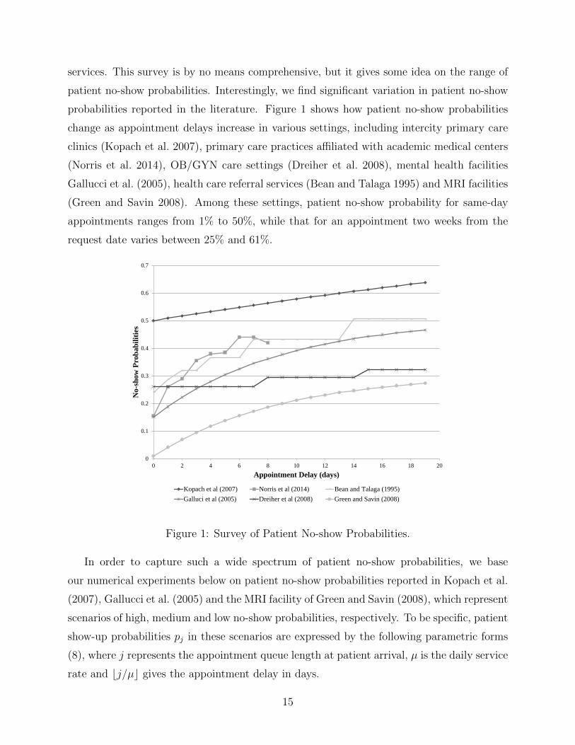
services. This survey is by no means comprehensive, but it gives some idea on the range of

patient no-show probabilities. Interestingly, we find significant variation in patient no-show

probabilities reported in the literature. Figure 1 shows how patient no-show probabilities

change as appointment delays increase in various settings, including intercity primary care

clinics (Kopach et al. 2007), primary care practices affiliated with academic medical centers

(Norris et al. 2014), OB/GYN care settings (Dreiher et al. 2008), mental health facilities

Gallucci et al. (2005), health care referral services (Bean and Talaga 1995) and MRI facilities

(Green and Savin 2008). Among these settings, patient no-show probability for same-day

appointments ranges from 1% to 50%, while that for an appointment two weeks from the

request date varies between 25% and 61%.

0

0.1

0.2

0.3

0.4

0.5

0.6

0.7

0 2 4 6 8 10 12 14 16 18 20

No-s

how

Pro

ba

bil

itie

s

Appointment Delay (days)

Kopach et al (2007) Norris et al (2014) Bean and Talaga (1995)

Galluci et al (2005) Dreiher et al (2008) Green and Savin (2008)

Figure 1: Survey of Patient No-show Probabilities.

In order to capture such a wide spectrum of patient no-show probabilities, we base

our numerical experiments below on patient no-show probabilities reported in Kopach et al.

(2007), Gallucci et al. (2005) and the MRI facility of Green and Savin (2008), which represent

scenarios of high, medium and low no-show probabilities, respectively. To be specific, patient

show-up probabilities pj in these scenarios are expressed by the following parametric forms

(8), where j represents the appointment queue length at patient arrival, µ is the daily service

rate and bj/µc gives the appointment delay in days.

15

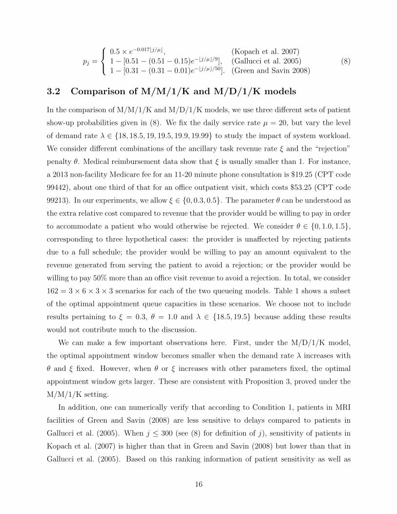
pj =

0.5× e−0.017bj/µc, (Kopach et al. 2007)1− [0.51− (0.51− 0.15)e−bj/µc/9], (Gallucci et al. 2005)1− [0.31− (0.31− 0.01)e−bj/µc/50]. (Green and Savin 2008)

(8)

3.2 Comparison of M/M/1/K and M/D/1/K models

In the comparison of M/M/1/K and M/D/1/K models, we use three different sets of patient

show-up probabilities given in (8). We fix the daily service rate µ = 20, but vary the level

of demand rate λ ∈ {18, 18.5, 19, 19.5, 19.9, 19.99} to study the impact of system workload.

We consider different combinations of the ancillary task revenue rate ξ and the “rejection”

penalty θ. Medical reimbursement data show that ξ is usually smaller than 1. For instance,

a 2013 non-facility Medicare fee for an 11-20 minute phone consultation is $19.25 (CPT code

99442), about one third of that for an office outpatient visit, which costs $53.25 (CPT code

99213). In our experiments, we allow ξ ∈ {0, 0.3, 0.5}. The parameter θ can be understood as

the extra relative cost compared to revenue that the provider would be willing to pay in order

to accommodate a patient who would otherwise be rejected. We consider θ ∈ {0, 1.0, 1.5},corresponding to three hypothetical cases: the provider is unaffected by rejecting patients

due to a full schedule; the provider would be willing to pay an amount equivalent to the

revenue generated from serving the patient to avoid a rejection; or the provider would be

willing to pay 50% more than an office visit revenue to avoid a rejection. In total, we consider

162 = 3× 6× 3× 3 scenarios for each of the two queueing models. Table 1 shows a subset

of the optimal appointment queue capacities in these scenarios. We choose not to include

results pertaining to ξ = 0.3, θ = 1.0 and λ ∈ {18.5, 19.5} because adding these results

would not contribute much to the discussion.

We can make a few important observations here. First, under the M/D/1/K model,

the optimal appointment window becomes smaller when the demand rate λ increases with

θ and ξ fixed. However, when θ or ξ increases with other parameters fixed, the optimal

appointment window gets larger. These are consistent with Proposition 3, proved under the

M/M/1/K setting.

In addition, one can numerically verify that according to Condition 1, patients in MRI

facilities of Green and Savin (2008) are less sensitive to delays compared to patients in

Gallucci et al. (2005). When j ≤ 300 (see (8) for definition of j), sensitivity of patients in

Kopach et al. (2007) is higher than that in Green and Savin (2008) but lower than that in

Gallucci et al. (2005). Based on this ranking information of patient sensitivity as well as

16

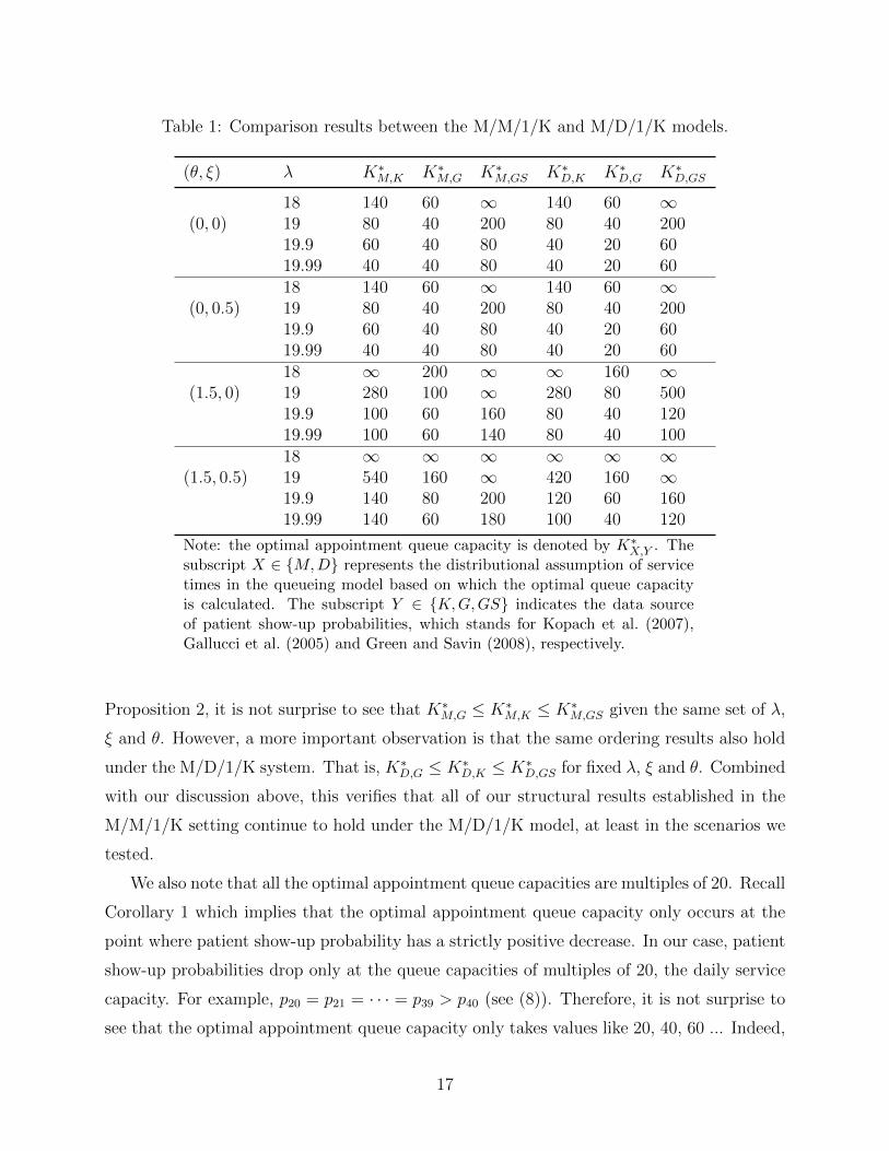
Table 1: Comparison results between the M/M/1/K and M/D/1/K models.

(θ, ξ) λ K∗M,K K∗M,G K∗M,GS K∗D,K K∗D,G K∗D,GS

(0, 0)18 140 60 ∞ 140 60 ∞19 80 40 200 80 40 20019.9 60 40 80 40 20 6019.99 40 40 80 40 20 60

(0, 0.5)18 140 60 ∞ 140 60 ∞19 80 40 200 80 40 20019.9 60 40 80 40 20 6019.99 40 40 80 40 20 60

(1.5, 0)18 ∞ 200 ∞ ∞ 160 ∞19 280 100 ∞ 280 80 50019.9 100 60 160 80 40 12019.99 100 60 140 80 40 100

(1.5, 0.5)18 ∞ ∞ ∞ ∞ ∞ ∞19 540 160 ∞ 420 160 ∞19.9 140 80 200 120 60 16019.99 140 60 180 100 40 120

Note: the optimal appointment queue capacity is denoted by K∗X,Y . Thesubscript X ∈ {M,D} represents the distributional assumption of servicetimes in the queueing model based on which the optimal queue capacityis calculated. The subscript Y ∈ {K,G,GS} indicates the data sourceof patient show-up probabilities, which stands for Kopach et al. (2007),Gallucci et al. (2005) and Green and Savin (2008), respectively.

Proposition 2, it is not surprise to see that K∗M,G ≤ K∗M,K ≤ K∗M,GS given the same set of λ,

ξ and θ. However, a more important observation is that the same ordering results also hold

under the M/D/1/K system. That is, K∗D,G ≤ K∗D,K ≤ K∗D,GS for fixed λ, ξ and θ. Combined

with our discussion above, this verifies that all of our structural results established in the

M/M/1/K setting continue to hold under the M/D/1/K model, at least in the scenarios we

tested.

We also note that all the optimal appointment queue capacities are multiples of 20. Recall

Corollary 1 which implies that the optimal appointment queue capacity only occurs at the

point where patient show-up probability has a strictly positive decrease. In our case, patient

show-up probabilities drop only at the queue capacities of multiples of 20, the daily service

capacity. For example, p20 = p21 = · · · = p39 > p40 (see (8)). Therefore, it is not surprise to

see that the optimal appointment queue capacity only takes values like 20, 40, 60 ... Indeed,

17

this is a convenient feature for converting the optimal appointment queue capacity into the

optimal appointment scheduling window (in days). To do so, one only needs to divide the

optimal appointment queue capacity by the daily service capacity, which is 20 in this case,

and always gets an integer number of days for the appointment scheduling window.

To examine how “close” an M/M/1/K model approximates an M/D/1/K system in mak-

ing suggestions for the optimal appointment scheduling window, we note that the M/M/1/K

model is able to make exactly the same suggestion as the M/D/1/K model in 28 out of the 72

scenarios we studied. For the rest of 44 cases, we evaluate the efficiency loss in the M/D/1/K

model due to using the optimal appointment window suggested by the M/M/1/K model.

Specifically, the efficiency loss is evaluated as 100%× [T (K∗D)−T (K∗M)]/T (K∗D), where T (·)is the reward function defined in (2) for M/D/1/K systems, and K∗M and K∗D respectively

represent the optimal appointment queue capacities calculated based on the M/M/1/K and

M/D/1/K settings. The average efficiency loss in these 44 scenarios is only 0.14% and the

maximum efficiency loss is 0.97%, suggesting that using the optimal appointment window

suggested by the M/M/1/K model in the M/D/1/K model only leads to negligible efficiency

loss. Thus the M/M/1/K model is a fairly accurate approximation for the more realistic

M/D/1/K system in terms of suggesting the optimal appointment scheduling window.

3.3 Efficiency gains resulted from adopting K∗

In this section, we study how much efficiency gain can be achieved by adopting an optimal

appointment scheduling window when practices may or may not use other operational levers.

3.3.1 Cases when practice cannot adjust panel size or overbooking level

This section deals with the case in which a practice cannot adjust its panel size or over-

booking level. Our numerical experiments use similar parameter settings as in Section 3.2.

Specifically, we use three different sets of patient no-show probabilities defined in (8). We

fix µ = 20 and vary λ ∈ {18, 19, 19.9, 19.99}, ξ ∈ {0, 0.3, 0.5} and θ ∈ {0, 1.0, 1.5}. Different

arrival rates λ represent different levels of workload ranging from lightly utilized to extremely

congested. We evaluate the efficiency gains based on both M/M/1/K and M/D/1/K models.

For a given queueing model and a fixed set of parameters, we assess the long-run average

net reward obtained by the system when patients can be scheduled any time into the future,

i.e., we calculate T (K) defined in (2) for K =∞. Then, we evaluate the long-run average net

reward when an optimal appointment window is used. That is, we calculate T (K∗) in which

18

K∗ is a maximizer to T (K). The efficiency gain is defined as the percentage improvement in

long-run average net reward obtained due to optimizing the appointment scheduling window,

i.e., 100%×[T (K∗)−T (∞)]/T (∞). A subset of the representative results are shown in Table

2 (please refer to Table 4 in the online Appendix for all numerical results).

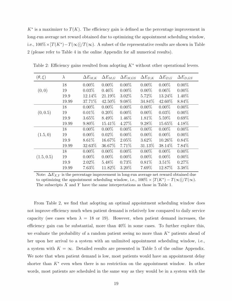
Table 2: Efficiency gains resulted from adopting K∗ without other operational levers.

(θ, ξ) λ ∆EM,K ∆EM,G ∆EM,GS ∆ED,K ∆ED,G ∆ED,GS

(0, 0)18 0.00% 0.00% 0.00% 0.00% 0.00% 0.00%19 0.03% 0.46% 0.00% 0.00% 0.06% 0.00%19.9 12.14% 21.19% 3.02% 5.72% 13.24% 1.40%19.99 37.71% 42.50% 9.08% 34.84% 42.60% 8.84%

(0, 0.5)18 0.00% 0.00% 0.00% 0.00% 0.00% 0.00%19 0.01% 0.20% 0.00% 0.00% 0.03% 0.00%19.9 3.65% 8.49% 1.46% 1.81% 5.59% 0.69%19.99 9.80% 15.41% 4.27% 9.28% 15.65% 4.18%

(1.5, 0)18 0.00% 0.00% 0.00% 0.00% 0.00% 0.00%19 0.00% 0.02% 0.00% 0.00% 0.00% 0.00%19.9 8.61% 16.67% 2.05% 3.62% 10.26% 0.84%19.99 32.63% 36.67% 7.71% 31.13% 38.14% 7.84%

(1.5, 0.5)18 0.00% 0.00% 0.00% 0.00% 0.00% 0.00%19 0.00% 0.00% 0.00% 0.00% 0.00% 0.00%19.9 2.02% 5.48% 0.73% 0.81% 3.51% 0.27%19.99 7.63% 11.82% 3.20% 7.69% 12.87% 3.38%

Note: ∆EX,Y is the percentage improvement in long-run average net reward obtained dueto optimizing the appointment scheduling window, i.e., 100% × [T (K∗) − T (∞)]/T (∞).The subscripts X and Y have the same interpretations as those in Table 1.

From Table 2, we find that adopting an optimal appointment scheduling window does

not improve efficiency much when patient demand is relatively low compared to daily service

capacity (see cases when λ = 18 or 19). However, when patient demand increases, the

efficiency gain can be substantial, more than 40% in some cases. To further explore this,

we evaluate the probability of a random patient seeing no more than K∗ patients ahead of

her upon her arrival to a system with an unlimited appointment scheduling window, i.e.,

a system with K = ∞. Detailed results are presented in Table 5 of the online Appendix.

We note that when patient demand is low, most patients would have an appointment delay

shorter than K∗ even when there is no restriction on the appointment window. In other

words, most patients are scheduled in the same way as they would be in a system with the

19

optimal appointment window in place. Consequently, restricting the appointment window

to be K∗ has limited impact on system efficiency. On the contrary, when patient demand

is high, only a small percentage of patients have an appointment delay shorter than K∗ in

a system with an unlimited appointment window. As it turns out, adopting an optimal

appointment window in this case can effectively reduce appointment delay, control no-show

rates and significantly improve efficiency.

We also note that the efficiency gains become smaller when the “rejection” penalty θ

or the ancillary task revenue rate ξ is larger. These observations are in line with what

Proposition 3 suggests. As θ or ξ increases, K∗ would also increase and therefore T (K∗)

gets closer to T (∞) resulting in a smaller efficiency gain. More importantly, we observe

that efficiency gains are more sensitive to the changes in ξ than in θ within the range of

parameter values we tested. This is likely due to the fact that revenue differentials between

patients scheduled in different times are highly sensitive to the value of ξ, and such revenue

differentials are the key driver for the optimal choice of appointment scheduling window (see

discussions in Section 2.2). As ξ increases, these revenue differentials drop quickly, making

it less effective to limit the appointment scheduling window.

3.3.2 Cases when practices may adjust panel size and overbooking level

In this section, we consider cases in which practices can adjust their panel size and over-

booking level freely. We adopt the same three sets of patient no-show probabilities as above,

and vary θ ∈ {0, 1.0, 1.5} and ξ ∈ (0, 0.3, 0.5) in our experiments. We consider both the

M/M/1/K and M/D/1/K queueing models. Given a queueing model and a fixed parameter

setup, we assume that the practice first optimizes its panel size and overbooking level fol-

lowing the model of Liu and Ziya (2014), which we briefly recapitulate below. In particular,

the practice solves the following optimization problem first.

maxλ,µ>0

λ∞∑j=0

Πj(λ, µ)qj + µ(1− ρ)ξ − ω(µ), (9)

where λ and µ are decision variables representing the demand rate (panel size) and service

rate (overbooking level) in the system, respectively. The variable ρ = λ/µ is the traffic

intensity, and Πj(λ, µ) represents the steady state probability that an incoming patient sees

j patients ahead upon her arrival for a given pair of λ and µ. Note that the objective

function above is essentially a special case of (2) with K = ∞ minus the last term ω(µ),

20

which represents the cost of providing the service. We adopt the form ω(µ) = a×[(µ−M)+]2

from Liu and Ziya (2014) in our experiments, and set the regular daily capacity M = 20

patients per day and the overtime cost parameter a ∈ {0.2, 2}. Thus if the practice chooses

µ to be larger than 20, it overbooks µ− 20 patients and incurs overtime cost ω(µ) per day.

After the practice solves the optimization problem (9) above and obtains the optimal

patient demand rate λ∗ and daily service capacity µ∗, it seeks the optimal appointment

window K∗ given (λ∗, µ∗). We evaluate the percentage efficiency gains resulted from further

adopting an optimal scheduling window in systems with the already optimized panel size and

overbooking level. As it turns out, when the overtime cost parameter a = 2, the practice

never overbooks, i.e., it always set µ∗ = M = 20. In this case, we can think of the practice

does not have an overbooking option (due to its high overtime cost) but can freely adjust

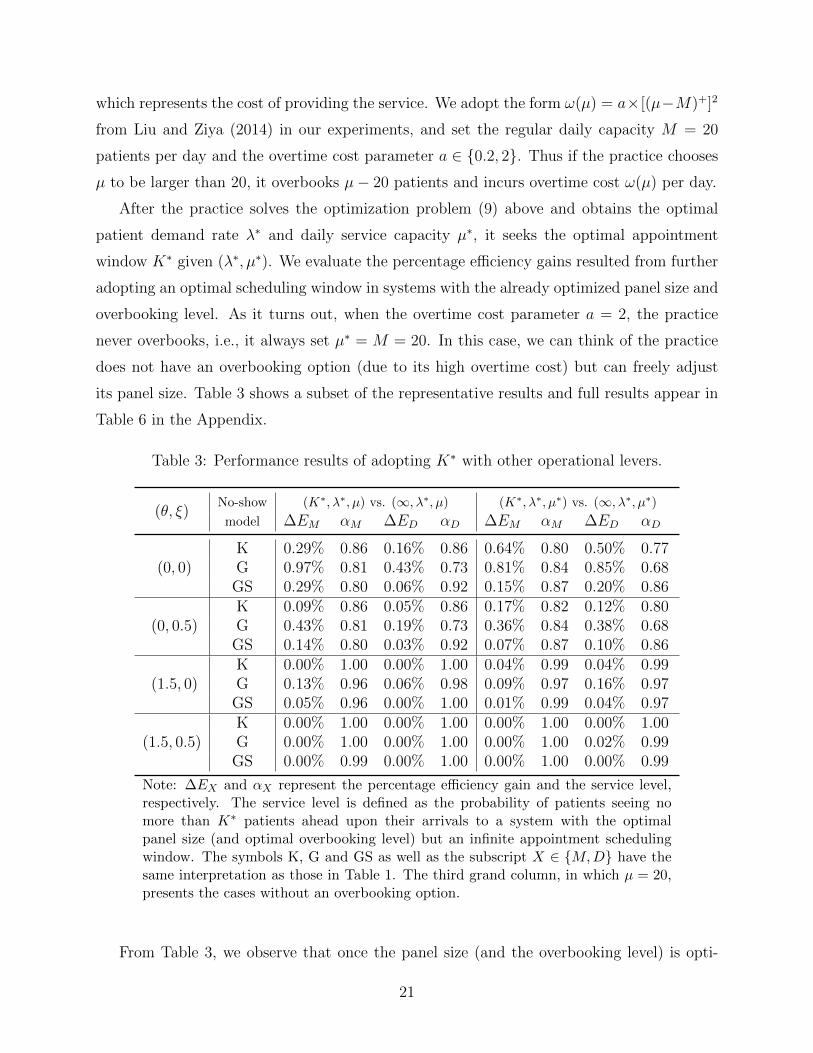
its panel size. Table 3 shows a subset of the representative results and full results appear in

Table 6 in the Appendix.

Table 3: Performance results of adopting K∗ with other operational levers.

(θ, ξ)No-show (K∗, λ∗, µ) vs. (∞, λ∗, µ) (K∗, λ∗, µ∗) vs. (∞, λ∗, µ∗)

model ∆EM αM ∆ED αD ∆EM αM ∆ED αD

(0, 0)K 0.29% 0.86 0.16% 0.86 0.64% 0.80 0.50% 0.77G 0.97% 0.81 0.43% 0.73 0.81% 0.84 0.85% 0.68

GS 0.29% 0.80 0.06% 0.92 0.15% 0.87 0.20% 0.86

(0, 0.5)K 0.09% 0.86 0.05% 0.86 0.17% 0.82 0.12% 0.80G 0.43% 0.81 0.19% 0.73 0.36% 0.84 0.38% 0.68

GS 0.14% 0.80 0.03% 0.92 0.07% 0.87 0.10% 0.86

(1.5, 0)K 0.00% 1.00 0.00% 1.00 0.04% 0.99 0.04% 0.99G 0.13% 0.96 0.06% 0.98 0.09% 0.97 0.16% 0.97

GS 0.05% 0.96 0.00% 1.00 0.01% 0.99 0.04% 0.97

(1.5, 0.5)K 0.00% 1.00 0.00% 1.00 0.00% 1.00 0.00% 1.00G 0.00% 1.00 0.00% 1.00 0.00% 1.00 0.02% 0.99

GS 0.00% 0.99 0.00% 1.00 0.00% 1.00 0.00% 0.99

Note: ∆EX and αX represent the percentage efficiency gain and the service level,respectively. The service level is defined as the probability of patients seeing nomore than K∗ patients ahead upon their arrivals to a system with the optimalpanel size (and optimal overbooking level) but an infinite appointment schedulingwindow. The symbols K, G and GS as well as the subscript X ∈ {M,D} have thesame interpretation as those in Table 1. The third grand column, in which µ = 20,presents the cases without an overbooking option.

From Table 3, we observe that once the panel size (and the overbooking level) is opti-

21

mized, the efficiency gains by further adopting an optimal appointment scheduling window

are limited (less than 1% in all scenarios). To explain this, we evaluate based on both

queueing models, the service level defined as the probability of patients seeing no more than

K∗ patients ahead upon their arrivals to a system with the optimal panel size (and opti-

mal overbooking level) but an infinite appointment scheduling window. K∗ is the optimal

appointment scheduling window that could be set given that the optimal panel size (and

overbooking level) is already in place. As we see in Table 3, these service levels are at least

68%, suggesting that optimizing the panel size (and the overbooking level) can already con-

trol patient appointment delay (and patient no-show rates) quite well. Further setting a

limit on the appointment window seeks to achieve a similar goal of influencing appointment

delays experienced by patients, and thus can only exert a limited impact.

3.4 Efficiency gains due to jointly optimizing all operational levers

To further explore the efficiency gain by controlling the appointment scheduling window,

we consider cases when practices can jointly optimize all operational levers: panel size,

overbooking level and appointment scheduling window. Specifically, the practice solves the

following optimization problem.

maxλ,µ>0,K∈Z+

λK−1∑j=0

Πj(λ, µ,K)qj + µξΠ0(λ, µ,K)− λθΠK(λ, µ,K)− ω(µ), (10)

in which Πj(λ, µ,K) represent the steady-state queue length for a given triplet of (λ, µ,K).

We adopt the same three sets of patient no-show probabilities as above, and vary θ ∈{0, 1.0, 1.5}, ξ ∈ (0, 0.3, 0.5) and a ∈ {0.2, 2} in our experiments. For convenience, we let

(K∗∗, λ∗∗, µ∗∗) represent the jointly optimal scheduling window, panel size and overbook-

ing level to (10). We evaluate the percentage efficiency gains due to using (K∗∗, λ∗∗, µ∗∗)

compared to using (K∗, λ∗, µ∗) obtained in Section (3.3.2) (see detailed results in Table 7

of the online Appendix). Except for the cases when θ = 0, the efficiency gains due to joint

optimization are almost zero. When θ = 0, i.e., when providers are not affected by “re-

jecting” patients due to a full schedule, the jointly optimal strategy appears to be using

a very large panel (ideally containing an infinite number of patients) and adopting a very

small appointment window (ideally one day), so that there are always patients in the system

whose appointment delay is minimal yielding the maximal possible revenues. Even with such

an unrealistic strategy, the M/D/1/K model estimates that the largest efficiency gain is no

22

more than 5% in all cases we tested. Therefore, taking together with our previous numerical

results, we may conclude that optimizing the appointment scheduling window serves more

as a substitute, rather than a complement, to optimizing the panel size (and overbooking

level).

4 Extension to Heterogeneous Customers

The previous sections deal with models with homogeneous customers. However, customers

with different personal characteristics may differ in their no-show probabilities. For instance,

patients who had missed their prior appointments tend to have a higher chance of break-

ing their future appointments (Norris et al. 2014). Observing this phenomenon, providers

may use different appointment windows for patients depending on their no-show behaviors

(Rosenthal 2011, DuMontier et al. 2013). In this section, we consider a simple stylized model

with heterogeneous customers to study such decision making. In particular, we assume that

there are two types of patients who differ in their arrival rates and show-up probabilities.

Type i patients join the queue according to a Poisson process with rate λi for i = 1, 2.

The probability that a type i patient will show up given j patients ahead of her upon her

appointment request is pij. Similar to our previous models, we assume that these show-up

probabilities decrease as patient appointment delay increases, i.e., pij ≥ pi,j+1 for i = 1, 2

and j = 0, 1, 2, . . . . We also assume that the provider knows exactly the patient type when

a patient arrives, and she may use patient type-specific appointment windows. That is, the

provider will not schedule type i patients if there are already Ki patients (regardless of their

types) in the system, where K1 can be different from K2.

Except for the differences above, these two types of customers are the same in other

aspects and model assumptions are also similar to those of the M/M/1/K model with ho-

mogeneous customers considered in Section 2. The service times of each customer are i.i.d.

exponential random variables with mean 1/µ. If the scheduled customer does not show up

for an appointment slot or there is no customer scheduled for that slot, the provider is able

to fill it by an ancillary task which yields a reward ξ ∈ [0, 1). Each patient served brings in

one nominal unit of reward and each unscheduled patient incurs a cost θ to the system. The

provider’s objective is to maximize the long-run average net reward by choosing K1 and K2

appropriately.

One can show that for this stylized model, the long-run average net reward given (K1, K2),

23

denoted as T (K1, K2), has a closed-form expression. To be specific, let ρ = (λ1 + λ2)/µ,

ρi = λi/µ, wi = λi/(λ1 + λ2), and rij = θ + (1 − ξ)pij for i = 1, 2, and j = 0, 1, 2, . . . . We

need to consider two cases separately: K2 ≥ K1 and K1 > K2. We use T (K1, K2|K2 ≥ K1)

to represent the long-run average net reward collected by the system given that K2 ≥ K1,

i.e., when the service provider allows a longer appointment scheduling window for type 2

customers. For convenience, we write T (K1, K2) = T (K1, K2|K2 ≥ K1). Similarly, we write

T (K1, K2|K1 ≥ K2) as T (K1, K2). Then, by modeling the number of scheduled appointments

in the system as a Continuous Time Markov Chain for each of the two cases, we can obtain

the following expressions for T (K1, K2) and T (K1, K2), respectively. Detailed derivations

are presented in the online Appendix.

T (K1, K2) =(λ1 + λ2)

∑K1−1j=0 ρj(w1r1,j + w2r2,j) + λ2ρ

K1∑K2−1

j=K1ρj−K1

2 r2,j∑K1

j=0 ρj + ρK1

∑K2−K1

j=1 ρj2+ µξ − (λ1 + λ2)θ,

and

T (K1, K2) =(λ1 + λ2)

∑K2−1j=0 ρj(w1r1,j + w2r2,j) + λ1ρ

K2∑K1−1

j=K2ρj−K2

1 r1,j∑K2

j=0 ρj + ρK2

∑K1−K2

j=1 ρj1+ µξ − (λ1 + λ2)θ.

Now we can evaluate the long-run average net reward T (K1, K2) for any (K1, K2) using

T (K1, K2) =

{T (K1, K2) if K1 > K2,

T (K1, K2) if K2 ≥ K1.

And the service provider’s problem can be formulated as

maxK1,K2∈Z+

T (K1, K2). (P2)

As discussed earlier, the service provider may either use the same appointment window for

them, or differentiate the appointment windows based on patient type. Below we consider

these two cases separately.

4.1 Case that requires K1 = K2

When the service provider choose to use the same appointment window, she simply sets K1 =

K2 as a constraint in problem (P2). The arrivals of both types of patients follow independent

Poisson processes with rates λ1 and λ2, respectively. Thus the joint arrival process is also a

Poisson process, with rate λ1 + λ2. The probability that an arriving patient belongs to type

i is wi (see Theorem 5.6 in Kulkarni (1995)). Therefore, for a random arrival who sees j

24

patients ahead of her, her expected show-up probability is pj = w1p1j+w2p2j, j = 0, 1, 2, . . . .

When K1 = K2, the number of patients registered in the system becomes an M/M/1/K1

queue. In this case, the model with heterogeneous customers simply reduces to a model

with homogeneous customers where λ and pj are replaced by λ1 + λ2 and pj, respectively.

Therefore, all results derived in Section 2 apply to this case.

4.2 Case that allows K1 6= K2

When the provider can freely choose appointment windows, intuition suggests that the

provider would be better off by offering a longer appointment scheduling window for cus-

tomers who have higher show-up probabilities, because these “better behaved” customers

can be held longer in the system while still having the same or higher show-up probabilities.

Indeed, such a scheduling paradigm is widely adopted in practice to deal with frequent no-

show offenders by offering them very short appointment windows (see Rosenthal (2011) and

DuMontier et al. (2013)). However, we have seen that the intuition above fails when cus-

tomers are homogeneous (or equivalently, when the provider does not know the patient type

information but can only treat every patient as a random draw from a patient population

with a common no-show probability distribution). In that case, solely improving customer

show-up rates does not guarantee a larger appointment scheduling window to be optimal

(see Example 1). Customer sensitivity to delays plays a more important role there. Could

customer sensitivity to delay play a similar role when customers are heterogeneous in their

no-show behavior and the provider knows exactly their type?

The following proposition provides some answer to the question above. It actually points

to a different result to the homogeneous case. When patients are heterogenous and the

provider knows exactly their type, it would be optimal for the provider to set a longer

appointment window for patients with higher show-up probabilities, irrespective of their

sensitivity to delays.

Proposition 4 If p1j ≤ p2j for j = 0, 1, 2, . . . , then there exists an optimal pair of the

appointment queue capacities (K∗1 , K∗2) such that K∗1 ≤ K∗2 .

To give an intuitive explanation for Proposition 4, imagine that the provider sets an

appointment window K1 for type 1 patients who have lower show-up probabilities. Suppose

that at this moment, the queue length is shorter than K1. If a type 1 patient arrives, the

provider would accept this patient to the system. If instead a type 2 patient comes at this

25

moment, the provider seems to have no reason to “reject” this patient as this patient has a

higher show-up probability than type 1 patients. Following this logic, the provider should

set K2 at least the same as K1.

In the proposition above, p1j ≤ p2j is the only required condition for this ordering result

to hold. It actually holds independently of all other model parameters, such as customer

arrival rates λ1 and λ2 and provider service rate µ. Put into the context of health care

management, Proposition 4 gives a robust ordering result that does not depend on patient

mix or practice size, indicating that as long as one group of patients have higher show-up

rates, allowing a longer appointment window for them can lead to better system performance.

5 Conclusion

Patients’ no-show behavior presents a significant problem faced by many health care providers.

Since patient no-show rates usually increase with their appointment delays, one commonly-

adopted operational strategy by providers is to control the length of the appointment window.

By limiting patients from making appointments too far away into the future, the provider re-

duces patient appointment delays and thus no-show rates. Although there is a growing body

of literature on various operational strategies to deal with patient no-shows, little is known

about the impact of varying appointment scheduling windows on a provider’s operational

efficiency. This paper is directed to fill this knowledge gap.

The key tradeoff here is between the efficiency loss due to high no-show rates follow-

ing from allowing a longer appointment window and the “penalty” resulted from an overly

restrictive appointment window driving too many patients unable to schedule their appoint-

ments. We capture this tradeoff by using a single server queue to model the appointments

registered in a provider’s work schedule. The capacity of the queue serves as a proxy of

the length of the appointment window. The provider wants to set a common appointment

window for all patients, who have higher no-show probabilities when their appointment de-

lays are longer, to maximize her long-run average net reward. Using a stylized M/M/1/K

queueing model, we provide analytical characterizations for the optimal appointment queue

capacity, and study how the optimal scheduling window should be adjusted in response to

changes in other model parameters. Via extensive numerical experiments, we confirm that

our analytical results continue to hold in more realistic settings. In addition, one particu-

larly useful message from our numerical study to practitioners is that adopting an optimal

26

appointment scheduling window can lead to substantial efficiency gains if the provider has no

other operational levers at hand to deal with patient no-shows. However, when the provider

can adjust panel size and overbooking level, limiting the appointment scheduling window

serves more as a substitute strategy, rather than a complement.

Our work points to several directions for future research. First, our model extension

studies a single server queue with two types of patients differing in their no-show probabilities.

The provider knows the type of each incoming patient, and may set different appointment

windows depending on patient type. These patient type-specific appointment windows,

however, are static over time and independent of the system state. A dynamic admission

policy which depends on the current patient composition in the queue or a policy that sets

a limit on the number of each type of patients in the system holds the promise of further

improving system efficiency. However, these variations would lead to completely different and

likely more challenging optimization problems, which we leave for future research. Second,

in our model with heterogeneous patients, we assume that providers can perfectly segment

patients based on their no-show probabilities. However, misclassification errors may occur in

reality and it is important to study how such errors can affect our analysis and results. Third,

our model is stylized in nature mainly for deriving managerial insights and more research is

needed to develop decision support tools for practical use. For example, patients may have

stronger preferences for convenient times of day rather than shorter appointment delays,

and thus they may not accept the earliest available appointment. In addition to no-shows,

patients may cancel in advance or reschedule their appointments. These patient behaviors

can leave “holes” in the appointment queue. In this case, a first-come-first-served queue may

not be an accurate representation. Thus, one avenue for future research is to examine the

connection between the appointment window size and the operational efficiency in a more

realistic setting. Analytical study based on stylized queueing models may be difficult, but

simulation experiments are likely to yield useful results.

Acknowledgments

The author is grateful to the departmental editor, the senior editor and the anonymous

referees, whose comments and suggestions have helped improve this work. The author also

thanks the audience at the workshop on Data-Driven Decisions in Healthcare organized

by the Statistical and Applied Mathematical Sciences Institute (SAMSI) in 2013 for their

27

useful feedback. This work was partially supported by the Calderone Junior Faculty Research

Award, Mailman School of Public Health, Columbia University.

References

Atun, R.A., S.R. Sittampalam, A. Mohan. 2005. Uses and benefits of SMS in healthcare

delivery. Working paper, Tanaka Business Sschool, Imperial College.

Bean, A. G., J. Talaga. 1995. Predicting appointment breaking. Journal of Health Care

Marketing 15(1) 29–34.

Cayirli, T., E. Veral. 2003. Outpatient scheduling in health care: A review of literature.

Production and Operations Management 12(4) 519–549.

Dreiher, J., M. Froimovici, Y. Bibi, D.A. Vardy, A. Cicurel, A.D. Cohen. 2008. Nonatten-

dance in obstetrics and gynecology patients. Gynecologic and Obstetric Investigation

66(1) 40–43.

DuMontier, C., K. Rindfleisch, J. Pruszynski, J. J. Frey III. 2013. A multi-method interven-

tion to reduce no-shows in an urban residency clinic. Family medicine 45(9) 634–41.

Gallucci, G., W. Swartz, F. Hackerman. 2005. Brief reports: Impact of the wait for an initial

appointment on the rate of kept appointments at a mental health center. Psychiatric

Services 56(3) 344–346.

Geraghty, M., F. Glynn, M. Amin, J. Kinsella. 2007. Patient mobile telephone text reminder:

a novel way to reduce non-attendance at the ENT out-patient clinic. The Journal of

Laryngology and Otology 122(3) 296–298.

Green, L. V., S. Savin. 2008. Reducing delays for medical appointments: A queueing ap-

proach. Operations Research 56(6) 1526–1538.

Gupta, D., B. Denton. 2008. Appointment scheduling in health care: Challenges and oppor-

tunities. IIE Transactions 40(9) 800–819.

Guy, R., J. Hocking, H. Wand, S. Stott, H. Ali, J. Kaldor. 2012. How effective are short mes-

sage service reminders at increasing clinic attendance? a meta-analysis and systematic

review. Health Services Research 47(2) 614–632.

Hashim, M. J. P. Franks, K. Fiscella. 2001. Effectiveness of telephone reminders in improving

rate of appointments kept at an outpatient clinic: a randomized controlled trial. The

Journal of the American Board of Family Practice 14(3) 193–196.

28

Hassin, R., S. Mendel. 2008. Scheduling arrivals to queues: A single-server model with

no-shows. Management Science 54(3) 565–572.

Kopach, R., P. C. DeLaurentis, M. Lawley, K. Muthuraman, L. Ozsen, R. Rardin, H. Wan,

P. Intrevado, X. Qu, D. Willis. 2007. Effects of clinical characteristics on successful open

access scheduling. Health Care Management Science 10(2) 111–124.

Kulkarni, V. G. 1995. Modeling and Analysis of Stochastic Systems . Chapman & Hall/CRC,

Boca Raton, FL.

LaGanga, L. R., S. R. Lawrence. 2007. Clinic overbooking to improve patient access and

increase provider productivity. Decision Sciences 38(2) 251–276.

Liu, N., S. Ziya. 2014. Panel size and overbooking decisions for appointment-based services

under patient no-shows. Production and Operations Management 23(12) 2209–2223.

Liu, N., S. Ziya, V. G. Kulkarni. 2010. Dynamic scheduling of outpatient appointments under

patient no-shows and cancellations. Manufacturing & Service Operations Management

12(2) 347–364.

Macharia, W. M., G. Leon, B. H. Rowe, B. J. Stephenson, R. B. Haynes. 1992. An overview

of interventions to improve compliance with appointment keeping for medical services.

The Journal of the American Medical Association 267(13) 1813–1817.

Merrell, Katie, Robert A Berenson. 2010. Structuring payment for medical homes. Health

Affairs 29(5) 852–858.

Moore, C. G., P. Wilson-Witherspoon, J. C. Probst. 2001. Time and money: Effects of

no-showsat a family practice residency clinic. Family Medicine 33(7) 522–527.

Murray, M., C. Tantau. 2000. Same-day appointments: Exploding the access paradigm.

Family Practice Management . September, 2000.

Muthuraman, K., M. Lawley. 2008. A stochastic overbooking model for outpatient clinical

scheduling with no-shows. IIE Transactions 40(9) 820–837.

Nguyen, D.L., R.S. DeJesus, M.L. Wieland. 2011. Missed appointments in resident continuity

clinic: Patient characteristics and health care outcomes. Journal of Graduate Medical

Education 3(3) 350–355.

Norris, J. B., C. Kumar, S. Chand, H. Moskowitz, S. A. Shade, D. R. Willis. 2014. An empir-

ical investigation into factors affecting patient cancellations and no-shows at outpatient

clinics. Decision Support Systems 57 428–443.

29

Patrick, J., M. L. Puterman, M. Queyranne. 2008. Dynamic multi-priority patient scheduling

for a diagnostic resource. Operations Research 56(6) 1507–1525.

Robinson, L. W., R. R. Chen. 2010. A comparison of traditional and open-access policies

for appointment scheduling. Manufacturing & Service Operations Management 12(2)

330–346.

Rosenthal, D. 2011. Director of Behavioral Science of Center for Family and Community

Medicine at Columbia University. Personal communication. March 16, 2011.

Rural Assistance Center. 2013. Federally Qualified Health Centers frequently asked

questions. Http://www.raconline.org/topics/federally-qualified-health-centers/faqs.

Accessed: August 9, 2014.

Schectman, J.M., J.B. Schorling, J.D. Voss. 2008. Appointment adherence and disparities in

outcomes among patients with diabetes. Journal of General Internal Medicine 23(10)

1685–1687.

Shin, P., J. Sharac, C. Alvarez, S. Rosenbaum. 2013. Community health centers in an era

of health reform: An overview and key challenges to health center growth executive

summary. The Kaiser Commission on Medicaid and the Uninsured March 2013.

U.S. Department of Health and Human Services. 2014. What

are Federally qualified health centers (FQHCs)? URL:

http://www.hrsa.gov/healthit/toolbox/RuralHealthITtoolbox/Introduction/qualified.html.

Accessed: August 9, 2014.

Zeng, B., A. Turkcan, J. Lin, M. Lawley. 2010. Clinic scheduling models with overbooking

for patients with heterogeneous no-show probabilities. Annals of Operations Research

178(1) 121–144.

30

Online Supplement for “Optimal Choice forAppointment Scheduling Window under Patient

No-show Behavior”

Nan Liu

Department of Health Policy and Management, Mailman School of Public Health, Columbia

University, New York, New York 10032, USA

nl2320@columbia.edu

A Proofs of the Results

Lemma 1 Let a, c ≥ 0 and b, d > 0. If a/b ≥ (>)c/d, then

c

d≤ (<)

a+ c

b+ d≤ (<)

a

b.

Proof of Lemma 1: We prove the first inequality. The proof for the second one is very

similar.

a

b≥ (>)

c

d⇔ bc ≤ (<)ad⇔ bc+ dc ≤ (<)ad+ dc⇔ c

d≤ (<)

a+ c

b+ d. �.

Lemma 2 Let a, c1, c2 ≥ 0 and b, d1, d2 > 0. If c2/d2 ≥ c1/d1 ≥ a/b, c2 ≥ c1 and d2 ≥ d1,

thena+ c2

b+ d2

≥ a+ c1

b+ d1

.

Proof of Lemma 2: It suffices to show that

(a+ c2)(b+ d1) ≥ (a+ c1)(b+ d2),

which is equivalent to

ab+ c2b+ d1a+ c2d1 ≥ ab+ c1b+ d2a+ c1d2.

It is clear that c2d1 ≥ c1d2 by the given assumption. Now it is left to show that

c2b+ d1a ≥ c1b+ d2a,

which is equivalent to

c2 − c1 ≥a

b(d2 − d1).

1

Let α = c1/d1. Then it follows that c2 ≥ d2α and α ≥ a/b. Therefore

c2 − c1 ≥ α(d2 − d1) ≥ a

b(d2 − d1),

completing the proof. �.

Proof of Proposition 1: Equation (6) implies that showing T (K) is unimodal in K is

equivalent to showing f(K) is unimodal in K. Similarly, showing that the largest maximizer

of T (K) is given by (7) is equivalent to showing that the largest maximizer of f(K) is given

by (7).

First, the set S is nonempty because 1 ∈ S for any ρ since f(0) = 0 < r0 = θ+ (1− ξ)p0.

Also note that f(1) = r0/(1 + ρ) ≥ f(0). Now, suppose that for some K ≥ 2, K ∈ S. That

is, f(K − 1) ≤ rK−1/ρ, or equivalently

f(K − 1) =

∑K−2j=0 ρjrj∑K−1i=0 ρi

≤ rK−1

ρ=ρK−1rK−1

ρK. (11)

Then, we have

f(K) =

∑K−2j=0 ρjrj + ρK−1rK−1∑K−1

i=0 ρi + ρK≥

∑K−2j=0 ρjrj∑K−1i=0 ρi

= f(K − 1), (12)

which follows from Lemma 1 and (11). These show that ∀K ∈ S, f(K) ≥ f(K − 1).

Now, suppose that supS < ∞, then we let K∗ = supS and show below that f(K)

strictly decreases in K if K > K∗. Using a symmetric argument to (11), (12) and Lemma 1

and noting that f(K∗) > rK∗/ρ by definition of S, we can show rK∗/ρ < f(K∗+1) < f(K∗).

Notice that rK∗+1 ≤ rK∗ since pj is decreasing in j. We conclude that rK∗+1/ρ < f(K∗+ 1),

which implies that f(K∗ + 2) < f(K∗ + 1). Continuing this argument, one can show that

f(K) strictly decreases in K if K > K∗. Thus S only contains consecutive integer numbers,

i.e., S = {1, 2, . . . , K∗}. It follows that f(K) increases up to K∗ and then strictly decreases

afterwards. Finally, if supS = ∞, then we can see that the optimal queueing capacity K∗

is infinity. The proof is complete. �

Proof of Corollary 1: Proof by constructing a contradiction. Suppose that at K = K∗,

rK = rK−1. Since K ∈ S, we know

rK−1

ρ=ρK−1rK−1

ρK≥ f(K − 1) =

∑K−2j=0 ρjrj∑K−1i=0 ρi

.

Using Lemma 1, we can show that

rKρ

=rK−1

ρ≥

∑K−2j=0 ρjpj + ρK−1rK−1∑K−1

i=0 ρi + ρK= f(K).

2

Thus K + 1 ∈ S and K∗ = supS ≥ K + 1 > K, leading to a contradiction and completing

the proof. �.

Proof of Proposition 2: Let rj = θ + pj(1− ξ). Define S as follows.

S = {K :

∑K−2j=0 ρj rj∑K−1i=0 ρi

≤ rK−1

ρ,K ∈ Z+}.

From (5) and Proposition 1, it is sufficient to show that S ⊇ S. Now, pick any K ∈ S,

which implies that rK−1 > 0. Condition 1 suggests that rK−1 ≥ rK−1 and hence rK−1 > 0.

We make the following claim, which will be proved at the end.

rjrK−1

≥ rjrK−1

, ,∀j = 0, 1, . . . , K − 1. (13)

It follows that ∑K−2j=0 ρj

rjrK−1∑K−1

i=0 ρi≤

∑K−2j=0 ρj

rjrK−1∑K−1

i=0 ρi≤ 1

ρ,

which immediately implies that K ∈ S and hence S ⊇ S.

Now, we prove the claim (13). It is sufficient to show that

rj rj+1 ≥ rj rj+1 for j = 0, 1, . . . , K − 1. (14)

Consider

rj rj+1 − rj rj+1 = [θ + (1− ξ)pj][θ + (1− ξ)pj+1]− [θ + (1− ξ)pj][θ + (1− ξ)pj+1]

= θ(1− ξ)[(pj+1 − pj)− (pj+1 − pj)] + (1− ξ)2(pj pj+1 − pjpj+1),

where the first term is nonnegative due to Condition 1. The second term can be rewritten

as

(1− ξ)2(pj pj+1 − pjpj+1) = (1− ξ)2(pj pj+1 − pj+1pj+1 + pj+1pj+1 − pjpj+1)

= (1− ξ)2[pj+1(pj − pj+1)− pj+1(pj − pj+1)] ≥ 0,

since pj+1 ≥ pj+1 ≥ 0 and pj − pj+1 ≥ pj − pj+1 ≥ 0 (by Condition 1). This completes the

proof. �.

Proof of Proposition 3:

Part (a): With a slight abuse of notation, we rewrite (5) for 1 ≤ K < ∞ as fK(ρ).

Accordingly, we rewrite the net reward function (6) as

TK(ρ) = λ(fK(ρ) +1

ρξ − θ). (15)

3

In (15), only the term fK(ρ) involves with K and thus other terms can be dropped when

we optimize it for K∗. We use K∗(λ) to represent K∗ for a fixed λ. With other parameters

being fixed, K∗(λ) decreases with λ if and only if K∗(ρ) decreases with ρ where K∗(ρ) is the

largest optimal choice of K for fK(ρ) defined in (15). Consider

fK+1(ρ)− fK(ρ) =ρK∑K

i=0 ρi∑K+1

j=0 ρjgK(ρ)

where

gK(ρ) = rK

K∑j=0

ρj − ρK−1∑j=0

ρjrj. (16)

Recall that rj = θ + (1 − ξ)pj for j ≥ 0. Since there exists 0 ≤ i < j such that pi > pj,

there also exists 0 ≤ i < j such that ri > rj. Let K = min{k : rk−1 > rk}. Corollary 1

implies that K∗(ρ) ≥ K for all ρ > 0. Also note that K∗(ρ) ≤ K = inf{j : rj = 0}. It is

clear that K ≥ K. We assume that K > K for otherwise K∗(ρ) = K for all ρ > 0 and the

result trivially holds.

Now, for any K ≤ K ≤ K − 1, taking the derivative of gK(ρ) with respect to ρ, we find

g′K(ρ) =K∑j=1

(rK − rj−1) j ρj−1 < 0,

as rK < rK−1. Therefore, gK(ρ) is a continuous and strictly decreasing function. Noting

that gK(0) = rK = θ + (1 − ξ)pK > 0 and limρ→∞ gK(ρ) = −∞, we can conclude that

gK(ρ) = 0 has exactly one real root on (0,∞), which we denote by ρK . It also follows that

TK+1(ρ) > TK(ρ) for any ρ < ρK and TK+1(ρ) < TK(ρ) for any ρ > ρK .

We consider two cases below. First, suppose that K + 1 = K. Then, K∗(ρ) = K if

ρ ≤ ρK−1 and K∗(ρ) = K otherwise. Thus, K∗(ρ) decreases in ρ.

Then, we consider the case K + 1 < K. Suppose that ρK+1 ≤ ρK for any K ≥ K. This

would imply that for any fixed ρ, K∗(ρ) = K + 1 if and only if ρK+1 < ρ ≤ ρK . Therefore,

as ρ increases K∗(ρ) can only get smaller and the desired results should follow. Hence, it

remains to show that ρK+1 ≤ ρK for any K ≤ K ≤ K − 1.

Using the fact that gK(ρK) = 0 and gK+1(ρK+1) = 0, we have

ρKr0 + ρ2Kr1 + . . . ρKKrK−1

rK + ρKrK + . . . ρKKrK= 1,

andρK+1r0 + ρ2

K+1r1 + . . . ρKK+1rK−1 + ρK+1K+1rK

rK+1 + ρK+1rK+1 + . . . ρKK+1rK+1 + ρK+1K+1rK+1

= 1. (17)

4

Suppose for contradiction that ρK+1 > ρK . Then, we must have gK(ρK+1) < 0, i.e.,

ρK+1r0 + ρ2K+1r1 + . . . ρKK+1rK−1

rK + ρK+1rK + . . . ρKK+1rK> 1.

Multiplying both sides by rK/rK+1, we get

ρK+1r0 + ρ2K+1r1 + . . . ρKK+1rK−1

rK+1 + ρK+1rK+1 + . . . ρKK+1rK+1

>rKrK+1

≥ 1.

Then, usingρK+1K+1rK

ρK+1K+1rK+1

=rKrK+1

≥ 1

together with Lemma 1, we find

ρK+1r0 + ρ2K+1r1 + . . . ρKK+1rK−1 + ρK+1

K+1rK

rK+1 + ρK+1rK+1 + . . . ρKK+1rK+1 + ρK+1K+1rK+1

> 1,

which is a contradiction to (17). This completes the proof of (a).

Part (b): Let K∗(µ) represent K∗ for a fixed µ. Note that with other parameters being

fixed, K∗(µ) increases with µ if and only if K∗(ρ) decreases with ρ where K∗(ρ) is the largest

optimal choice of K for fK(ρ) defined in (15). Then the result directly follows from (a).

Part (c): Let K∗(θ) represent K∗ for a fixed θ. Consider arbitrary θ ≥ θ ≥ 0. We

want to show that K∗(θ) ≥ K∗(θ). From (15), we see that changes in θ influences K∗ only

through fK(ρ). In fK(ρ), θ only affects rj’s. Let rj be defined as rj with θ replaced by θ.

Following the similar idea in the proof of Proposition 2, it suffices to show that

rj rj+1 ≥ rj rj+1 for j = 0, 1, 2, . . . .

Note that the definition of rj differs from that in the proof of Proposition 2. Consider

rj rj+1 − rj rj+1 = [θ + (1− ξ)pj][θ + (1− ξ)pj+1]− [θ + (1− ξ)pj][θ + (1− ξ)pj+1]

= (1− ξ)(θ − θ)(pj − pj+1) ≥ 0,

completing the proof of (c).

Part (d): The proof is similar to that of (c). Let K∗(ξ) represent K∗ for a fixed ξ.

Consider arbitrary ξ ≥ ξ ≥ 0. We want to show that K∗(ξ) ≥ K∗(ξ). With a slight abuse

of the notation, we let rj be defined as rj with ξ replaced by ξ. It suffices to show that

rj rj+1 ≥ rj rj+1 for j = 0, 1, 2, . . . .

5

Note that the definition of rj differs from that in the proofs of Part (c) and Proposition 2.

Consider

rj rj+1 − rj rj+1 = [θ + (1− ξ)pj][θ + (1− ξ)pj+1]− [θ + (1− ξ)pj][θ + (1− ξ)pj+1]

= θ[(1− ξ)− (1− ξ)](pj − pj+1) ≥ 0,

completing the proof. �.

Proof of Proposition 4: It is equivalent to show the following result: if p2j ≤ p1j for

j = 0, 1, 2, . . . , then there exists a pair of the optimal appointment queue capacities (K∗1 , K∗2)

such that K∗2 ≤ K∗1 . We choose to prove this result because we will be working with

T (K1, K2) = T (K1, K2) whereK2 ≥ K1 in this proof. This is consistent with the presentation

and proof of other results.

Now, suppose that p2j ≤ p1j and there exists one pair of the optimal capacities satisfying

K∗2 > K∗1 . Pick an arbitrary K ∈ {K∗1 , K∗ + 1, . . . , K∗2 − 1}. We will show that

T (K,K∗2) ≤ T (K + 1, K∗2), (18)

from which it would follow that T (K∗1 , K∗2) ≤ T (K∗2 , K

∗2) and thus (K∗2 , K

∗2) must also be

optimal, proving the desired result. To show (18), first let rj = w1r1j+w2r2j and λ = λ1+λ2.

Observe that

T (K,K∗2) =λ∑K−1

j=0 ρj rj + λ2ρK∑K∗

2−1j=K ρj−K2 r2,j∑K

j=0 ρj + ρK

∑K∗2−K

j=1 ρj2+ µξ − (λ1 + λ2)θ

=λ∑K−1

j=0 ρj rj + λ2ρKr2,K + λ2ρ

K∑K∗

2−1j=K+1 ρ

j−K2 r2,j∑K

j=0 ρj + ρKρ2 + ρK

∑K∗2−K

j=2 ρj2+ µξ − (λ1 + λ2)θ,(19)

and

T (K + 1, K∗2) =λ∑K−1

j=0 ρj rj + λρK rK + λ2ρK+1

∑K∗2−1

j=K+1 ρj−K−12 r2,j∑K

j=0 ρj + ρK+1 + ρK+1

∑K∗2−K−1

j=1 ρj2+ µξ − (λ1 + λ2)θ

≥λ∑K−1

j=0 ρj rj + λρKr2,K + λ2ρK+1

∑K∗2−1

j=K+1 ρj−K−12 r2,j∑K

j=0 ρj + ρK+1 + ρK+1

∑K∗2−K−1

j=1 ρj2+ µξ − (λ1 + λ2)θ.

6

The last inequality results from rK ≥ r2,K (since p2j ≤ p1j). Let

a = λK−1∑j=0

ρj rj, b =K∑j=0

ρj; (20)

c1 = λ2ρKr2,K + λ2ρ

K

K∗2−1∑

j=K+1

ρj−K2 r2,j, d1 = ρKρ2 + ρKK∗

2−K∑j=2

ρj2; (21)

c2 = λρKr2,K + λ2ρK+1

K∗2−1∑

j=K+1

ρj−K−12 r2,j, d2 = ρK+1 + ρK+1

K∗2−K−1∑j=1

ρj2, (22)

Then

T (K,K∗2) =a+ c1

b+ d1

+ µξ − (λ1 + λ2)θ

and

T (K + 1, K∗2) ≥ a+ c2

b+ d2

+ µξ − (λ1 + λ2)θ.

It is easy to check that

c2ρ2

ρ= c1, d2

ρ2

ρ= d1, and ρ ≥ ρ2,

and hence

c2 ≥ c1, d2 ≥ d1, andc1

d1

=c2

d2

.

We claim thatc1

d1

≥ a

b. (23)

Then a direct application of Lemma 2 yields the desired inequality (18).

We now proceed to prove (23). The optimality of (K∗1 , K∗2) implies that

T (K∗1 , K∗2) ≥ T (K,K) =

a

b+ µξ − (λ1 + λ2)θ,

and thusλ∑K∗

1−1j=0 ρj rj + λ2ρ

K∗1∑K∗

2−1j=K∗

1ρj−K∗

12 r2,j∑K∗

1j=0 ρ

j + ρK∗1

∑K∗2−K∗

1j=1 ρj2

≥ a

b. (24)

We denote the left hand side of (24) as L(K∗1 , K∗2), which can be rewritten as

L(K∗1 , K∗2) =

λ∑K∗

1−1j=0 ρj rj + λ2ρ

K∗1∑K−1

j=K∗1ρj−K∗

12 r2,j + λ2ρ

K∗1∑K∗

2−1j=K ρ

j−K∗1

2 r2,j∑K∗1

j=0 ρj + ρK

∗1

∑K−K∗1

j=1 ρj2 + ρK∗1

∑K∗2−K∗

1j=K+1−K∗

1ρj2

≥ a

b. (25)

Since (K∗1 , K∗2) is optimal, it follows from Proposition 5 (see below) and Lemma 1 that

λ2ρK∗

1ρK∗

2−K∗1−1

2 r2,K∗2−1

ρK∗1ρ

K∗2−K∗

12

= µr2,K∗2−1 ≥ L(K∗1 , K

∗2). (26)

7

Observe that the ratio of the last term in the numerator of L(K∗1 , K∗2) and the last term in

the denominator of L(K∗1 , K∗2) can be rewritten as

λ2ρK∗

1∑K∗

2−1j=K ρ

j−K∗1

2 r2,j

ρK∗1

∑K∗2−K∗

1j=K+1−K∗

1ρj2

=λ2ρ

K−K∗1

2

∑K∗2−1

j=K ρj−K2 r2,j

ρK−K∗

12

∑K∗2−K

j=1 ρj2=λ2

∑K∗2−1

j=K ρj−K2 r2,j∑K∗2−K

j=1 ρj2=c1

d1

. (27)

Noting that r2,j decreasing in j, we can continue (27) and and show

λ2

∑K∗2−1

j=K ρj−K2 r2,j∑K∗2−K

j=1 ρj2=c1

d1

=µ∑K∗

2−K−1j=0 ρj2r2,j+K∑K∗

2−K−1j=0 ρj2

≥ µ r2,K∗2−1. (28)

Finally, combining (24), (26), and (28) yields that

c1

d1

≥ µ r2,K∗2−1 ≥ L(K∗1 , K

∗2) ≥ a

b, (29)

proving our claim (23) and completing the proof. �.

Proposition 5 For any fixed λ1, λ2, µ,K1 > 0 and given that K2 ≥ K1, the net reward

T (K1, K2) is a quasi-concave function of K2 over K2 = K1, K1 + 1, . . . . Furthermore, the

largest maximizer K∗2 is given by

K∗2 = sup{K2 : K2 ∈ S2} (30)

where

S2 = {K2 : g(K2 − 1) ≤ µ r2,K2−1, K2 = K1 + 1, . . . } ∪ {K1}. (31)

Proof of Proposition 5:

For fixed K1, the optimal K2 to T (K1, K2) is optimal to g(K2), and vice versa. Observe that

g(K2) =(λ1 + λ2)

∑K1−1j=0 ρj(w1r1,j + w2r2,j) + λ2ρ

K1∑K2−1

j=K1ρj−K1

2 r2,j∑K1

j=0 ρj + ρK1

∑K2−K1

j=1 ρj2

=N(K1, K2 − 1) + λ2ρ

K1ρK2−K1−12 r2,K2−1

D(K1, K2 − 1) + ρK1ρK2−K12

.

Notice thatλ2ρ

K1ρK2−K1−12 r2,K2−1

ρK1ρK2−K12

= µ r2,K2−1,

which is decreasing in K2. Following a similar logic in the proof of Proposition 1, one can

show that g(K2) is non-decreasing in K2 until g(K2 − 1) > µr2,K2−1, completing the proof.

�.

8

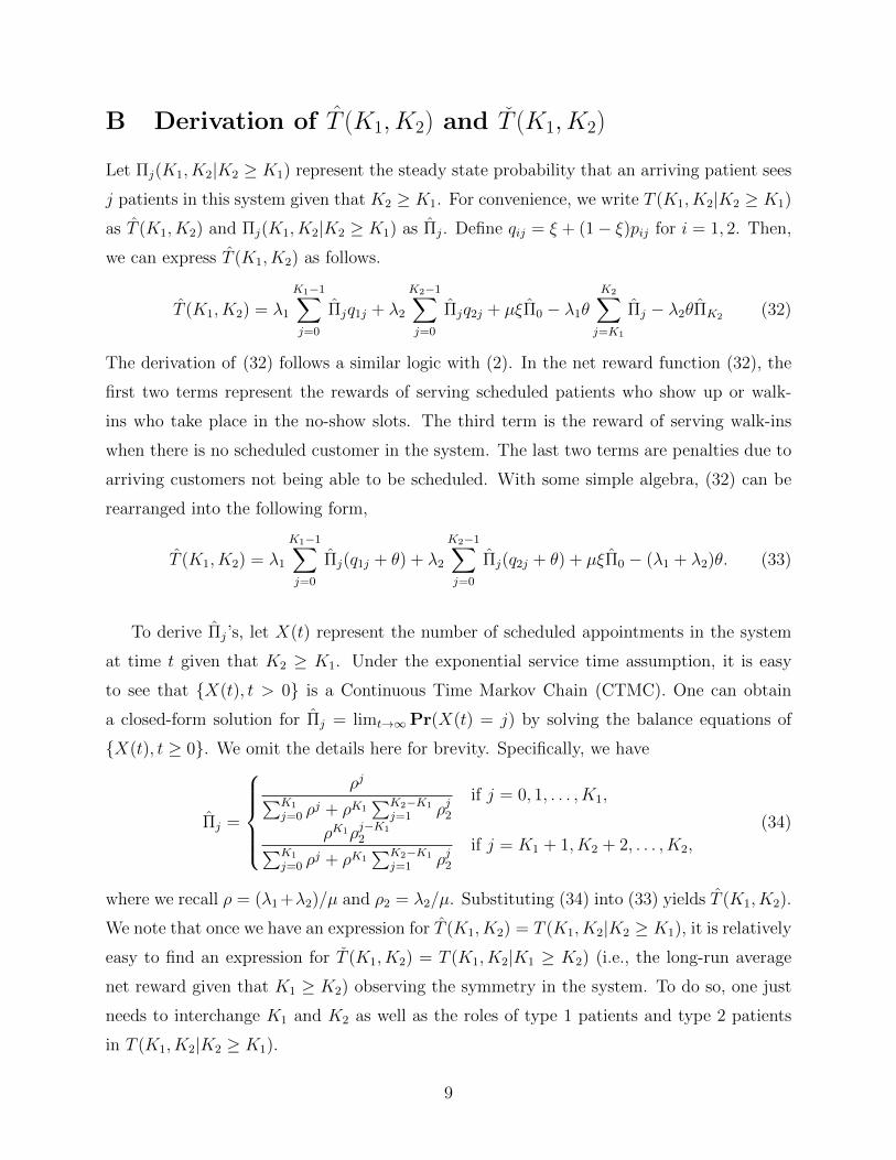
B Derivation of T (K1, K2) and T (K1, K2)

Let Πj(K1, K2|K2 ≥ K1) represent the steady state probability that an arriving patient sees

j patients in this system given that K2 ≥ K1. For convenience, we write T (K1, K2|K2 ≥ K1)

as T (K1, K2) and Πj(K1, K2|K2 ≥ K1) as Πj. Define qij = ξ + (1− ξ)pij for i = 1, 2. Then,

we can express T (K1, K2) as follows.

T (K1, K2) = λ1

K1−1∑j=0

Πjq1j + λ2

K2−1∑j=0

Πjq2j + µξΠ0 − λ1θ

K2∑j=K1

Πj − λ2θΠK2 (32)

The derivation of (32) follows a similar logic with (2). In the net reward function (32), the

first two terms represent the rewards of serving scheduled patients who show up or walk-

ins who take place in the no-show slots. The third term is the reward of serving walk-ins

when there is no scheduled customer in the system. The last two terms are penalties due to

arriving customers not being able to be scheduled. With some simple algebra, (32) can be

rearranged into the following form,

T (K1, K2) = λ1

K1−1∑j=0

Πj(q1j + θ) + λ2

K2−1∑j=0

Πj(q2j + θ) + µξΠ0 − (λ1 + λ2)θ. (33)

To derive Πj’s, let X(t) represent the number of scheduled appointments in the system

at time t given that K2 ≥ K1. Under the exponential service time assumption, it is easy

to see that {X(t), t > 0} is a Continuous Time Markov Chain (CTMC). One can obtain

a closed-form solution for Πj = limt→∞Pr(X(t) = j) by solving the balance equations of

{X(t), t ≥ 0}. We omit the details here for brevity. Specifically, we have

Πj =

ρj∑K1

j=0 ρj + ρK1

∑K2−K1

j=1 ρj2if j = 0, 1, . . . , K1,

ρK1ρj−K1

2∑K1

j=0 ρj + ρK1

∑K2−K1

j=1 ρj2if j = K1 + 1, K2 + 2, . . . , K2,

(34)

where we recall ρ = (λ1 +λ2)/µ and ρ2 = λ2/µ. Substituting (34) into (33) yields T (K1, K2).

We note that once we have an expression for T (K1, K2) = T (K1, K2|K2 ≥ K1), it is relatively

easy to find an expression for T (K1, K2) = T (K1, K2|K1 ≥ K2) (i.e., the long-run average

net reward given that K1 ≥ K2) observing the symmetry in the system. To do so, one just

needs to interchange K1 and K2 as well as the roles of type 1 patients and type 2 patients

in T (K1, K2|K2 ≥ K1).

9

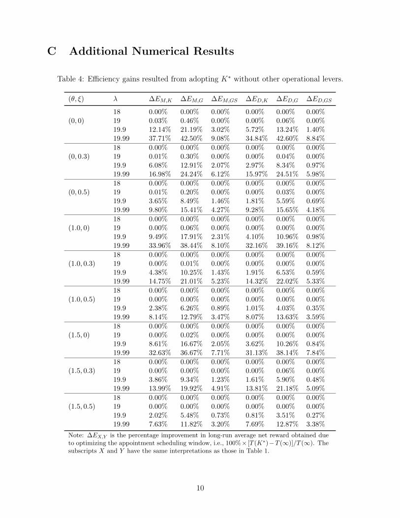
C Additional Numerical Results

Table 4: Efficiency gains resulted from adopting K∗ without other operational levers.

(θ, ξ) λ ∆EM,K ∆EM,G ∆EM,GS ∆ED,K ∆ED,G ∆ED,GS

(0, 0)18 0.00% 0.00% 0.00% 0.00% 0.00% 0.00%19 0.03% 0.46% 0.00% 0.00% 0.06% 0.00%19.9 12.14% 21.19% 3.02% 5.72% 13.24% 1.40%19.99 37.71% 42.50% 9.08% 34.84% 42.60% 8.84%

(0, 0.3)18 0.00% 0.00% 0.00% 0.00% 0.00% 0.00%19 0.01% 0.30% 0.00% 0.00% 0.04% 0.00%19.9 6.08% 12.91% 2.07% 2.97% 8.34% 0.97%19.99 16.98% 24.24% 6.12% 15.97% 24.51% 5.98%

(0, 0.5)18 0.00% 0.00% 0.00% 0.00% 0.00% 0.00%19 0.01% 0.20% 0.00% 0.00% 0.03% 0.00%19.9 3.65% 8.49% 1.46% 1.81% 5.59% 0.69%19.99 9.80% 15.41% 4.27% 9.28% 15.65% 4.18%

(1.0, 0)18 0.00% 0.00% 0.00% 0.00% 0.00% 0.00%19 0.00% 0.06% 0.00% 0.00% 0.00% 0.00%19.9 9.49% 17.91% 2.31% 4.10% 10.96% 0.98%19.99 33.96% 38.44% 8.10% 32.16% 39.16% 8.12%

(1.0, 0.3)18 0.00% 0.00% 0.00% 0.00% 0.00% 0.00%19 0.00% 0.01% 0.00% 0.00% 0.00% 0.00%19.9 4.38% 10.25% 1.43% 1.91% 6.53% 0.59%19.99 14.75% 21.01% 5.23% 14.32% 22.02% 5.33%

(1.0, 0.5)18 0.00% 0.00% 0.00% 0.00% 0.00% 0.00%19 0.00% 0.00% 0.00% 0.00% 0.00% 0.00%19.9 2.38% 6.26% 0.89% 1.01% 4.03% 0.35%19.99 8.14% 12.79% 3.47% 8.07% 13.63% 3.59%

(1.5, 0)18 0.00% 0.00% 0.00% 0.00% 0.00% 0.00%19 0.00% 0.02% 0.00% 0.00% 0.00% 0.00%19.9 8.61% 16.67% 2.05% 3.62% 10.26% 0.84%19.99 32.63% 36.67% 7.71% 31.13% 38.14% 7.84%

(1.5, 0.3)18 0.00% 0.00% 0.00% 0.00% 0.00% 0.00%19 0.00% 0.00% 0.00% 0.00% 0.06% 0.00%19.9 3.86% 9.34% 1.23% 1.61% 5.90% 0.48%19.99 13.99% 19.92% 4.91% 13.81% 21.18% 5.09%

(1.5, 0.5)18 0.00% 0.00% 0.00% 0.00% 0.00% 0.00%19 0.00% 0.00% 0.00% 0.00% 0.00% 0.00%19.9 2.02% 5.48% 0.73% 0.81% 3.51% 0.27%19.99 7.63% 11.82% 3.20% 7.69% 12.87% 3.38%

Note: ∆EX,Y is the percentage improvement in long-run average net reward obtained dueto optimizing the appointment scheduling window, i.e., 100%× [T (K∗)−T (∞)]/T (∞). Thesubscripts X and Y have the same interpretations as those in Table 1.

10

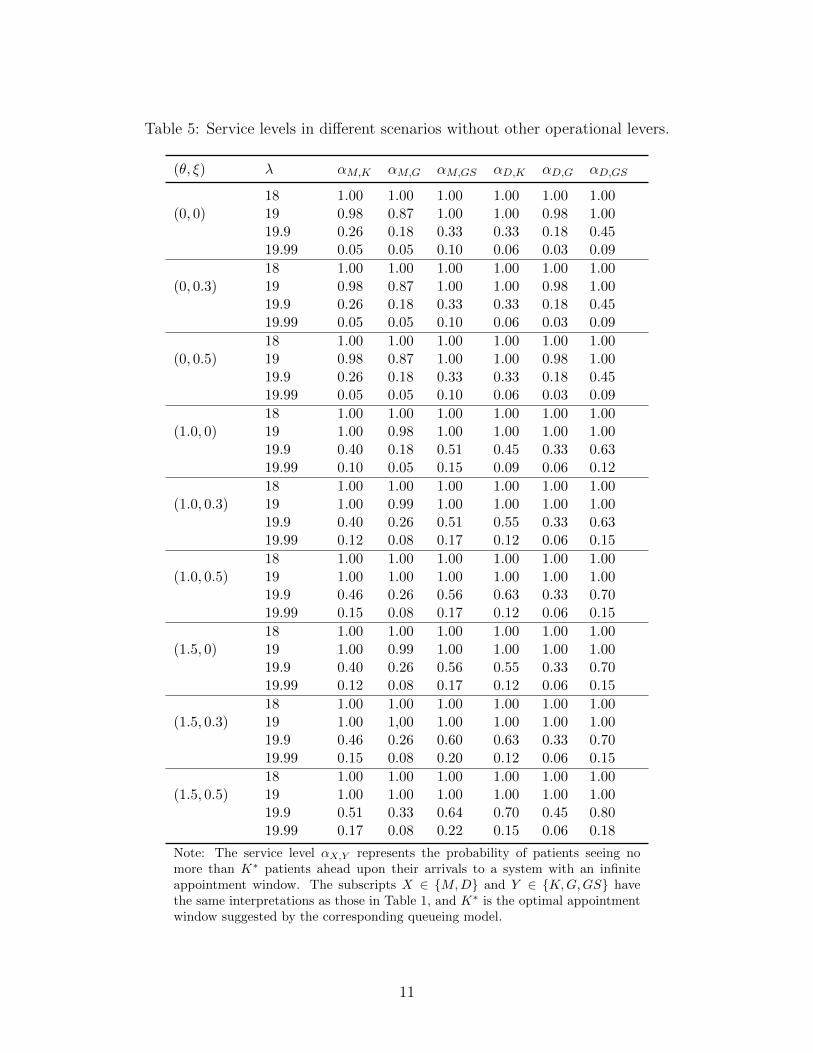
Table 5: Service levels in different scenarios without other operational levers.

(θ, ξ) λ αM,K αM,G αM,GS αD,K αD,G αD,GS

(0, 0)18 1.00 1.00 1.00 1.00 1.00 1.0019 0.98 0.87 1.00 1.00 0.98 1.0019.9 0.26 0.18 0.33 0.33 0.18 0.4519.99 0.05 0.05 0.10 0.06 0.03 0.09

(0, 0.3)18 1.00 1.00 1.00 1.00 1.00 1.0019 0.98 0.87 1.00 1.00 0.98 1.0019.9 0.26 0.18 0.33 0.33 0.18 0.4519.99 0.05 0.05 0.10 0.06 0.03 0.09

(0, 0.5)18 1.00 1.00 1.00 1.00 1.00 1.0019 0.98 0.87 1.00 1.00 0.98 1.0019.9 0.26 0.18 0.33 0.33 0.18 0.4519.99 0.05 0.05 0.10 0.06 0.03 0.09

(1.0, 0)18 1.00 1.00 1.00 1.00 1.00 1.0019 1.00 0.98 1.00 1.00 1.00 1.0019.9 0.40 0.18 0.51 0.45 0.33 0.6319.99 0.10 0.05 0.15 0.09 0.06 0.12

(1.0, 0.3)18 1.00 1.00 1.00 1.00 1.00 1.0019 1.00 0.99 1.00 1.00 1.00 1.0019.9 0.40 0.26 0.51 0.55 0.33 0.6319.99 0.12 0.08 0.17 0.12 0.06 0.15

(1.0, 0.5)18 1.00 1.00 1.00 1.00 1.00 1.0019 1.00 1.00 1.00 1.00 1.00 1.0019.9 0.46 0.26 0.56 0.63 0.33 0.7019.99 0.15 0.08 0.17 0.12 0.06 0.15

(1.5, 0)18 1.00 1.00 1.00 1.00 1.00 1.0019 1.00 0.99 1.00 1.00 1.00 1.0019.9 0.40 0.26 0.56 0.55 0.33 0.7019.99 0.12 0.08 0.17 0.12 0.06 0.15

(1.5, 0.3)18 1.00 1.00 1.00 1.00 1.00 1.0019 1.00 1,00 1.00 1.00 1.00 1.0019.9 0.46 0.26 0.60 0.63 0.33 0.7019.99 0.15 0.08 0.20 0.12 0.06 0.15

(1.5, 0.5)18 1.00 1.00 1.00 1.00 1.00 1.0019 1.00 1.00 1.00 1.00 1.00 1.0019.9 0.51 0.33 0.64 0.70 0.45 0.8019.99 0.17 0.08 0.22 0.15 0.06 0.18

Note: The service level αX,Y represents the probability of patients seeing nomore than K∗ patients ahead upon their arrivals to a system with an infiniteappointment window. The subscripts X ∈ {M,D} and Y ∈ {K,G,GS} havethe same interpretations as those in Table 1, and K∗ is the optimal appointmentwindow suggested by the corresponding queueing model.

11

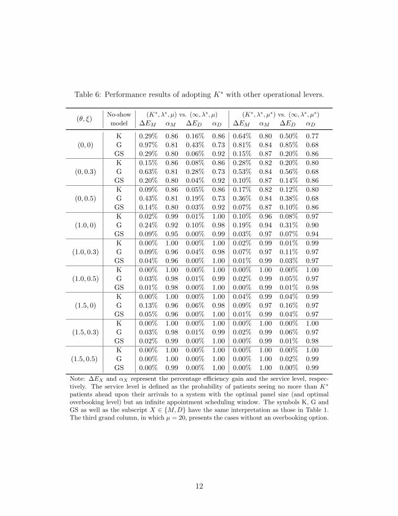
Table 6: Performance results of adopting K∗ with other operational levers.

(θ, ξ)No-show (K∗, λ∗, µ) vs. (∞, λ∗, µ) (K∗, λ∗, µ∗) vs. (∞, λ∗, µ∗)

model ∆EM αM ∆ED αD ∆EM αM ∆ED αD

(0, 0)K 0.29% 0.86 0.16% 0.86 0.64% 0.80 0.50% 0.77G 0.97% 0.81 0.43% 0.73 0.81% 0.84 0.85% 0.68

GS 0.29% 0.80 0.06% 0.92 0.15% 0.87 0.20% 0.86

(0, 0.3)K 0.15% 0.86 0.08% 0.86 0.28% 0.82 0.20% 0.80G 0.63% 0.81 0.28% 0.73 0.53% 0.84 0.56% 0.68

GS 0.20% 0.80 0.04% 0.92 0.10% 0.87 0.14% 0.86

(0, 0.5)K 0.09% 0.86 0.05% 0.86 0.17% 0.82 0.12% 0.80G 0.43% 0.81 0.19% 0.73 0.36% 0.84 0.38% 0.68

GS 0.14% 0.80 0.03% 0.92 0.07% 0.87 0.10% 0.86

(1.0, 0)K 0.02% 0.99 0.01% 1.00 0.10% 0.96 0.08% 0.97G 0.24% 0.92 0.10% 0.98 0.19% 0.94 0.31% 0.90

GS 0.09% 0.95 0.00% 0.99 0.03% 0.97 0.07% 0.94

(1.0, 0.3)K 0.00% 1.00 0.00% 1.00 0.02% 0.99 0.01% 0.99G 0.09% 0.96 0.04% 0.98 0.07% 0.97 0.11% 0.97

GS 0.04% 0.96 0.00% 1.00 0.01% 0.99 0.03% 0.97

(1.0, 0.5)K 0.00% 1.00 0.00% 1.00 0.00% 1.00 0.00% 1.00G 0.03% 0.98 0.01% 0.99 0.02% 0.99 0.05% 0.97

GS 0.01% 0.98 0.00% 1.00 0.00% 0.99 0.01% 0.98

(1.5, 0)K 0.00% 1.00 0.00% 1.00 0.04% 0.99 0.04% 0.99G 0.13% 0.96 0.06% 0.98 0.09% 0.97 0.16% 0.97

GS 0.05% 0.96 0.00% 1.00 0.01% 0.99 0.04% 0.97

(1.5, 0.3)K 0.00% 1.00 0.00% 1.00 0.00% 1.00 0.00% 1.00G 0.03% 0.98 0.01% 0.99 0.02% 0.99 0.06% 0.97

GS 0.02% 0.99 0.00% 1.00 0.00% 0.99 0.01% 0.98

(1.5, 0.5)K 0.00% 1.00 0.00% 1.00 0.00% 1.00 0.00% 1.00G 0.00% 1.00 0.00% 1.00 0.00% 1.00 0.02% 0.99

GS 0.00% 0.99 0.00% 1.00 0.00% 1.00 0.00% 0.99

Note: ∆EX and αX represent the percentage efficiency gain and the service level, respec-tively. The service level is defined as the probability of patients seeing no more than K∗

patients ahead upon their arrivals to a system with the optimal panel size (and optimaloverbooking level) but an infinite appointment scheduling window. The symbols K, G andGS as well as the subscript X ∈ {M,D} have the same interpretation as those in Table 1.The third grand column, in which µ = 20, presents the cases without an overbooking option.

12

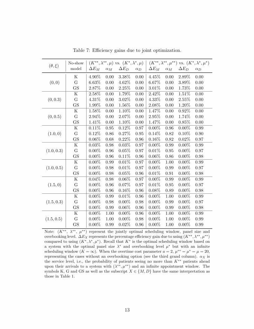
Table 7: Efficiency gains due to joint optimization.

(θ, ξ)No-show (K∗∗, λ∗∗, µ) vs. (K∗, λ∗, µ) (K∗∗, λ∗∗, µ∗∗) vs. (K∗, λ∗, µ∗)model ∆EM αM ∆ED αD ∆EM αM ∆ED αD

(0, 0)K 4.90% 0.00 3.38% 0.00 4.45% 0.00 2.89% 0.00G 6.63% 0.00 4.62% 0.00 6.67% 0.00 3.89% 0.00

GS 2.87% 0.00 2.25% 0.00 3.01% 0.00 1.73% 0.00

(0, 0.3)K 2.58% 0.00 1.79% 0.00 2.42% 0.00 1.51% 0.00G 4.31% 0.00 3.02% 0.00 4.33% 0.00 2.55% 0.00

GS 1.99% 0.00 1.56% 0.00 2.08% 0.00 1.20% 0.00

(0, 0.5)K 1.58% 0.00 1.10% 0.00 1.47% 0.00 0.92% 0.00G 2.94% 0.00 2.07% 0.00 2.95% 0.00 1.74% 0.00

GS 1.41% 0.00 1.10% 0.00 1.47% 0.00 0.85% 0.00

(1.0, 0)K 0.11% 0.95 0.12% 0.97 0.00% 0.96 0.00% 0.99G 0.12% 0.86 0.27% 0.95 0.14% 0.82 0.10% 0.90

GS 0.06% 0.68 0.22% 0.96 0.16% 0.82 0.02% 0.97

(1.0, 0.3)K 0.03% 0.98 0.03% 0.97 0.00% 0.99 0.00% 0.99G 0.00% 0.96 0.05% 0.97 0.01% 0.95 0.00% 0.97

GS 0.00% 0.96 0.11% 0.96 0.06% 0.86 0.00% 0.98

(1.0, 0.5)K 0.00% 0.99 0.01% 0.97 0.00% 1.00 0.00% 0.99G 0.00% 0.98 0.01% 0.97 0.00% 0.99 0.00% 0.97

GS 0.00% 0.98 0.05% 0.96 0.01% 0.91 0.00% 0.98

(1.5, 0)K 0.04% 0.98 0.06% 0.97 0.00% 0.99 0.00% 0.99G 0.00% 0.96 0.07% 0.97 0.01% 0.95 0.00% 0.97

GS 0.00% 0.96 0.16% 0.96 0.08% 0.89 0.00% 0.98

(1.5, 0.3)K 0.00% 0.99 0.01% 0.96 0.00% 1.00 0.00% 0.99G 0.00% 0.98 0.00% 0.98 0.00% 0.99 0.00% 0.97

GS 0.00% 0.99 0.06% 0.96 0.00% 0.99 0.00% 0.98

(1.5, 0.5)K 0.00% 1.00 0.00% 0.96 0.00% 1.00 0.00% 0.99G 0.00% 1.00 0.00% 0.98 0.00% 1.00 0.00% 0.99

GS 0.00% 0.99 0.02% 0.96 0.00% 1.00 0.00% 0.99

Note: (K∗∗, λ∗∗, µ∗∗) represent the jointly optimal scheduling window, panel size andoverbooking level. ∆EX represents the percentage efficiency gain due to using (K∗∗, λ∗∗, µ∗∗)compared to using (K∗, λ∗, µ∗). Recall that K∗ is the optimal scheduling window based ona system with the optimal panel size λ∗ and overbooking level µ∗ but with an infinitescheduling window (K =∞). When the overtime cost parameter a = 2, µ∗∗ = µ∗ = µ = 20,representing the cases without an overbooking option (see the third grand column). αX isthe service level, i.e., the probability of patients seeing no more than K∗∗ patients aheadupon their arrivals to a system with (λ∗∗, µ∗∗) and an infinite appointment window. Thesymbols K, G and GS as well as the subscript X ∈ {M,D} have the same interpretation asthose in Table 1.

13