OPTIMAL BROILER PRODUCTION VIA NUTRITION by
73
OPTIMAL BROILER PRODUCTION VIA NUTRITION by NUNTAWADEE SRIPERM (Under the Direction of Michael E. Wetzstein) ABSTRACT Today’s nutritionists employ the concept of dietary balanced protein (BP) in feed formulation in order to minimize the excess of crude protein and amino acids contents in broiler diets, which also minimize feed cost, while at the same time maintain broiler growth performance. The BP concept is when other AAs are set relative to lysine, thus, the main focus of this research was on lysine, especially at digestibility level in poultry. For that reason, the digestible lysine (dLys) levels were discussed throughout this research. The analysis was done using a dose-titrations trial. The data were used to evaluate the optimal economic dLys level to maximize profits using linear and nonlinear programming. The Cobb-Douglas functional form was proposed as an alternative model for performing production functions. The optimum responses were a function of current market prices of whole carcass or cut-up parts, and feed ingredients. The optimum dLys level during grower and finisher phases were determined and used to formulate the most profitable diets at a given targeted market and price scenario. The historical prices of major feed ingredients were used to evaluate the impact of low and high volatile prices to maximize profit under optimum feeding condition. INDEX WORDS: Dietary Balanced Protein, Digestible Lysine, Maximum Profit, Broiler Production, Linear and Nonlinear programming
Transcript of OPTIMAL BROILER PRODUCTION VIA NUTRITION by


x
LIST OF FIGURES
FIGURE PAGE
3.1 Graphical illustration of a one input production function……….………………………. 21
3.2 Graphical illustration of output isoquants of two inputs production function…………... 22
4.1 Historical corn and soybean meal prices and their spread (soybean meal price
minus corn price) between January 2000 and April 2011………………………………. 50
4.2 Probability distributions of maximum profit conditions during low (January
2000 to December 2005) and high (January 2006 to April 2011) volatile periods……... 51

1
CHAPTER 1
INTRODUCTION
1.1 Background Information
In broiler production, feed ingredient costs account for 60 to 70% of the overall
production costs (Agristat, 2010). Least-cost feed formulation is a common method to formulate
broiler diets; it minimizes feed costs at given feed ingredients and nutritional values. However,
nutrient requirements of this method always assume constant profits. Furthermore, the method
does not determine the output for each formulated diet regarding broiler performance. This
output can vary depending on the maximum profit of feeding the formulated diet to broilers
under various feed ingredient and broiler market prices. Profitability can be improved when
revenue and costs are both considered in the formulation of broiler diets. Broiler growth and feed
intake are two key components in determining the profit, which are not considered in least-cost
feed formulation.
About one-third of the feed ingredient cost comes from ingredients that purposely
provide the nutritional content to meet crude protein (CP) and amino acid (AA) requirements of
broilers. Thus, decreasing the excess of CP and AA contents based on the bird’s requirement
would improve feed formulation efficiency, which eventually reduces production costs.
Replacing soybean meal (SBM) with supplemental AA is a method to minimize the excess of CP
and AA contents. When SBM is replaced with supplemental AA, some of the AA (essential and
non essential AA) levels has been removed which also reduces CP levels. Determining the levels

2
of supplemental AA to maintain or improve growth performance has been widely studied.
However, earlier systems of listing broiler requirements for all essential AA at various stages of
growth and maintenance were difficult to follow. These led to research focusing on a better
solution by using the optimal proportion of the other AA to just one AA (say, lysine) (Baker et
al., 2002; Emmert and Baker, 1997; Mack et al., 1999; Wijtten et al., 2004). Thus, today
nutritionists employ the dietary balanced protein (BP) or ideal protein concept or ideal amino
acid ratios as all essential amino acids are held in ratios to lysine. Lysine has been selected
because it is a second-limiting AA in corn-soybean meal diets for poultry. It is only used for
protein synthesis, and is relatively easy to assay. Moreover, dietary lysine does not interact
metabolically with any other amino acids and is used primarily for protein accretion, not as a
precursor for other functions, unlike methionine (D'Mello, 2003).
When modeling the response to BP, the key amino acids are kept proportional to dietary
lysine levels such as the response measured by Baker, et al. (2002) and Lemme et al (2008).
Moreover, the needs for the essential and non-essential amino acids as well should be accounted
for. Diets containing low dietary lysine in early development result in reducing breast meat
formation because protein accretion from protein synthesis and RNA content decline (Tesseraud
et al., 1996). Thus, dietary lysine is more precise to use as a target in feed formulation compared
with crude protein which is an indirect calculation from the lab, by determination of nitrogen
level. Digestible lysine level (dLys) is addressed within this thesis. It does not mean only lysine
level was considered, but also represents the nutrient density of the diet. Hence the "optimal
nutrient density" or the "derived recommendation" is really the point of maximum economic
efficiency. Because it was an economic measure, it will change with changing economic
conditions.
3
A profit maximization model is developed in this research to evaluate the optimum
feeding levels of dLys, based on a balanced protein concept, where input (corn and SBM) and
output (whole carcass or cut-up parts) prices are varied. The consumer preferences for processed
chicken were also accounted in the model. The preferences varied from consuming whole
carcasses to cut-up parts, which were sold as frozen or seasoned by chicken producers or local
grocery stores. The optimum dLys levels, which provided the maximum profit, for this research
were determined from both sides of the production and processing of chicken. Thus, the input
and output markets are considered in the analysis and provide the effective feeding levels to meet
the consumer preferences or demand.
The model is operated under Microsoft Excel® spreadsheet. The spreadsheet makes the
analysis accessible to chicken producers and integrators. The spreadsheet can focus producers’
decision making when facing major input and output price volatility. The model can determine
the optimum conditions where a producer utilizes its production, inputs, and processing plant to
obtain the maximum profit.
1.2 Research Objectives
The research within this thesis is conducted to determine the maximum broiler
profitability, efficient feed compositions based on BP or ideal amino acid ratios for a particular
commercial broiler strain. Emphasis is placed on determining the optimal dLys level of two
feeding periods, grower and finisher phases based on variations in production costs and meat
prices. Given the price of live broilers, the broiler grower can determine the economically
efficient method to produce broilers. This research will be able to help the broiler growers and
nutritionists to determine nutrient levels, estimated body weight and feed consumption that
would provide the most profitability at certain days of grow-out.

4
The optimum BP of broilers production uses a Cobb-Douglas functional form, as a
growth function, to solve for maximum BW as a function of dLys levels during the grower and
finisher phases. The experimental data used in this research were based on nutrient dose-
response experimental data of Sriperm and Pesti (2011). Variations of feed ingredients and
broiler market prices were used to estimate the optimum dLys levels which maximize profit.
1.3 Brief Overview of Thesis
The review of economic theory on production functions, profit maximization, and
mathematical programming will be discussed. This review is useful in explaining how the profit-
maximizing nutrient levels, body weight, and feed intake are determined in the programming
model. An experimental data was used to obtain the data necessary to evaluate the broiler
production responses (body weight and feed intake) of dietary balanced protein (based on
digestible lysine level). The experiment was based on a specific broiler strain (Ross 708) with
male birds during 15 to 49 days. Different scenarios of feed ingredient and live broiler prices and
historical prices of major feed ingredients were discussed. The optimum nutrient levels during
grower (15 to 34 days) and finisher (35 to 49 days) phases were determined. The method used in
this research provides a broiler producer company a useful guideline in formulating profit-
maximizing diet and decision making for broiler growers.

5
CHAPTER 2
LITERATURE REVIEW
2.1 Balanced Dietary Amino Acids in Broiler Diets
Protein consists of at least 20 different amino acids (AA) bound together by peptide
bonds between the carboxyl and amino groups of adjacent AAs (Garrett and Grisham, 2007). In
poultry, ten AAs are required via the diet as called essential or indispensible AAs. They are
methionine, lysine, threonine, tryptophan, arginine, valine, isoleucine, leucine, histidine, and
phenylalanine. The remaining AAs are called non-essential or dispensable AAs, which poultry
are able to synthesize; these are glutamate, glutamine, glycine, serine, alanine, aspartate,
asparagines, cystine, tyrosine, and proline (D'Mello, J. 2003). In poultry, methionine is the first-
limiting AA, lysine is the second-limiting AA, threonine is the third-limiting AA, valine is the
fourth-limiting AA in corn-soybean meal diets without animal by-products (Corzo, 2008), and
tryptophan is the fourth-limiting AA in corn-soybean meal diets with meat blend of poultry meal,
meat and bone meal, and feather meal (Kidd and Hackenhaar, 2006). Lysine requirement has
been considered as a basis target, at the proper ratios of the other AA, in poultry feed
formulation. This was mainly due to protein synthesis, which is a primary function of lysine in
the body, lysine is relatively easy to assay, and it is not involved in any other biochemical
pathways, unlike methionine (D'Mello, J. 2003).
Dietary Balanced Protein (BP) or Ideal Protein (IP) or Ideal Amino Acid (IAA) ratios are
basically the same concept of using lysine as the reference AA. By setting the other AA as a

6
proportion to lysine requirement, the other AA can be easily calculated. The ideal AA ratios
would not change based on environmental (such as temperature, stress, and disease), dietary (low
or high CP or energy), and gender, while the other AA and lysine requirements would change
(D'Mello, J. 2003). Thus, lysine requirement is important to determine under different rearing
environments, diet and gender, while ideal AA ratios can be derived via previous
recommendations.
2.2 Profit Maximization Models for Broiler Production
2.2.1 Linear Programming
Least-cost feed formulation is a common method of formulating diets for broilers; it
minimizes the feed cost at given feed ingredients and their nutritional values. On the other hand,
nutrient requirements of this method always assume constant profits. Additionally, the method
does not determine the output for each formulated diet regarding broiler performance. The output
can be changed depending on the maximum profit of feeding the formulated diet to broilers
under various feed ingredient and broiler market prices. The profitability can be improved when
the revenue and cost are jointly considered in the formulation of broiler diets. The traditional
least-cost feed formulation using linear programming (LP) has been applied to formulate broiler
diets at a given set of nutrient requirements (Allison and Baird, 1974; Brown and Arscott, 1960).
A common objective of the formulations is to maximize bird performance (body weight (BW) or
feed efficiency) by determining the least-cost ration. A shortcoming of a LP is not considering
optimal bird performance in the production period. Although, the concept of a 95% asymptote
has been applied to the maximum nutrient requirement, to ensure the safety margin of the
formulated feed, it is still unknown whether the set requirements yield the profit maximum.
Allison and Baird (1974) reported that the concept of LP was to minimize feed ingredient costs,

7
which provided maximum performance regardless of feed ingredient prices. Feed nutrients, such
as AA, were set at a minimum constraint in order to provide the maximum animal performance.
Brown and Arscott (1960) estimated BW and feed consumption (FC) production functions in
calculating the optimum ration specification, CP and metabolizable energy (ME) contents. Using
a quadratic model to fit to the average data of 24 pens, they predicted BW as a function of CP
and ME consumed. The predicted pounds of FC per bird was measured as a function of time, CP
and ME content per pound of feed. A variable, measured as feeding period, was specified to
interacted with the feed composition terms, CP and ME contents, because time is required for
feed consumption regardless of feed composition. the resulting FC model was used to estimate
pounds of feed consume per bird at given CP and ME contents for a variety of feeding periods.
The LP was applied to calculate least-cost feed mixtures for various CP and ME specifications.
The margins over feed cost for these various points on the production surface were calculated.
Then, the highest profit was selected at the ration specification.
2.2.2 Nonlinear Programming
Pesti et al. (1986) proposed a quadratic response surface model of energy and protein to
estimate growth responses. Quadratic programing was used to evaluate the optimum operation
points in broiler production. The optimum operation points were defined as maximizing
production or live body weight at a given fixed level of cost (feed cost per bird) and a set of
inequality constraints on nutrients and feed ingredients. Economic theory was used to illustrate
how the model estimated cost per pound of broiler production within a specific time interval and
broiler quality (measured by carcass fat). They applied the law of diminising returns which states
as nutrient levels increased, the bird performance increased at a decreasing rate. Least-cost feed
formulation was studied under changing prices of corn and SBM affected CP and energy levels,

8
which minimized cost per pound of meat. They concluded that quadratic programming can
determine the most profitable CP and energy levels at variation in feed ingredient prices.
Talpaz et al. (1988) proposed a dynamic model to select the economically optimal growth
trajectory of broilers. They also computed the feeding schedule that satisfies the nutritional
requirements along this trajectory. They used nonlinear programming to determine the optimum
growth path for a broiler and considered the essential AA profile for maintenance and
requirement as major variables to evaluate optimum growth. Dynamic least-cost rations for the
potential growth rate, subject to the nutritional requirement, were determined. The model
estimated the daily optimal growth rates along with the corresponding requirements of total
protein, amino acids, and energy in obtaining the optimal diets. Result indicated that as feed
ingredient prices increased, more feed restrictions reduced the corresponding optimal growth
trajectory. Thus, a substantial increase in profits can be achieved by following their
methodology.
Gonzalez-Alcorta et al. (1994) used nonlinear programming techniques to determine the
precise energy and protein levels that maximize profits. The BW and cumulative FI functions
were generated as a quadratic function of energy and protein levels and age of the birds at time
of processing. They found that as the price of corn increased, the energy level decreased and
protein level increased. In addition, as the price of SBM increased, the protein level decreased
while the energy level increased. They concluded that setting CP and energy levels at various
input and output prices could increase profits compared with fixed levels of CP and energy based
on nutritional guideline.
Costa et al. (2001) developed a two step profit-maximization model based on minimizing
feed cost while maximizing revenue in broiler production. The minimizing feed cost was

9
determined at the optimal feed consumed, feed cost, and overall production cost, which included
cost of growing broilers, optimal length of time that the broilers stay in the house and interest
rate. The maximum revenue was estimated at various broiler prices, either whole carcass or cut-
up part prices, and optimum live or processed BW of the birds. Profit maximization was
estimated at the optimal protein levels, which provided minimizing feed cost while maximizing
revenue. They compared peanut meal as an alternative protein source for SBM and concluded
that using peanut meal could generate more profit for growing broiler compare with SBM.
Guevara (2004) proposed nonlinear programming over the conventional linear
programming to optimize broiler performance response to energy density in feed formulation
because the energy level does not need to be set. The BW and FC were fit to quadratic equations
in terms of energy density. The optimal ME level and bird performance were estimated by using
Excel solver nonlinear programming. The variation in corn, SBM, fish meal and broiler prices
were used. The nonlinear programming indicated that when the protein ingredient prices
decreased, the energy density increased compared with the linear programming least cost
formulation. The increased broiler price had a positive impact to BW and feed conversion and
also increased energy density. The conclusion was that nonlinear programming can be used to
define the optimal feed mix which maximizes margin over feed cost.
Eits et al. (2005b) focused on evaluating margin over feed costs (revenue minus feed
costs). This return over investment concept as shown by Eits et al. (2005b) is the difference
between increasing feed costs with increasing nutrient density and the decreasing incremental
technical performance response from increasing nutrient density. Their model indicated the
effect of dietary balanced protein on revenue and feed costs and from the difference of the two

10
the margins over feed costs. The idea behind maximizing profitability through nutrition is to
formulate the optimal nutrient density which maximizes profit.
Sterling et al. (2005) applied a quadratic growth response equation to estimate BW gain
as a function of dietary lysine and CP intake using a quadratic programming model. The program
was used to estimate maximum profit feed formulation and provided a working tool to
demonstrate the interdependencies of costs, technical response functions and meat prices. Based
on the quadratic programming model, increasing the price of SBM decreased CP and Lys level
that gave maximum BW gain. They concluded that using maximum profit model instead of least
cost model could generate improved profits.
Cerrate and Waldroup (2009a) proposed a maximum profit feed formulation model as an
alternative for least-cost feed formulation. Based on Ross male performance, BW and cut-up
parts were used to determine changes in dietary nutrient density which was the level of
metabolizable energy (ME). The models accounted for livability, temperature, processing cost,
ingredient and broiler prices, starting and ending broiler prices. The relative BW and feed
consumption (FC) were estimated using a quadratic function of ME at 49 days of age. The
absolute BW was estimated from the final day of feeding (49 days of age) using a Gompertz
equation, while the absolute FC was predicted from the absolute BW using a quadratic equation.
Carcass weight was calculated from the actual BW and yield (as a quadratic function of ME at
63 days of age). Cut-up parts were calculated by the multiplication of carcass weight and the
constant of each cut-up part. They found that as the price of poultry fat increased, the ME level
tended to decrease drastically, which reduced the usage of poultry fat and SBM in the diet while
increasing the usage of corn. Their model had higher profits compared with least cost and
provided improved profits when poultry oil prices increased by 150%.
11
Cerrate and Waldroup (2009b) compared four different economic nutritional models for
maximum profit feed formulation of broilers. As there are many methods of feed formulation:
consider the ratio of energy and some nutrients such as protein (Gonzalez-Alcorta et al., 1994);
or increase protein and AA levels while maintaining constant energy levels (Eits et al. (2005a,b);
or increase energy levels while maintaining AA and CP (Dozier III et al., 2006). The different
feed formulation methods certainly provided different growth performance. The four models,
which represented different methods of feed formulation, were a constant calorie-nutrient ratio
(C-E:P: Model 1), a variable calorie-protein ratio (V-E:Pg: Model 2), a constant protein-amino
acid ratio (DBP: Model 3) and a variable calorie-protein ratio for the finisher period (V-E:Pd:
Model 4).
Using relative performance, economic nutrient requirements, and profitability to compare
the four models. Cerrate and Waldroup (2009b) found that changing feed ingredient prices had
some impact on the enery and protein contents based on the four models. For example, as corn or
broiler price increased, the energy and protein contents of model 1-3 increased except the energy
content of model 2 decreased. The opposite was found when SBM or poultry oil (fat) price
increased. They concluded that model 1 was dominant in terms of feed formulation that
provided the maximum performance and profitability. Model 4 dominated in terms of profits as
well but with a narrow range of price changes and inconsistency of growth responses. Model 3
can be used at low corn or high SBM prices. The data set of Model 1 came from the past ten
years that contained a new strain of birds and responses to increasing all the nutrients. Thus, the
predicted BW from Model 1 was higher than Models 2 and 3, which resulted in the most
profitable model. They commented that modern broilers with rapid growth do not adjust feed
consumption to meet a fixed energy need. This resulted in the birds eating more energy as the

12
energy content increased, especially when AA and CP increased along with the energy.
However, when AA and CP were kept constant, the increase of energy content reduced feed
consumption to balance the energy intake.
2.3 An Alternative Production Function: the Cobb-Douglas Production Function
According to Douglas (1976), the Cobb-Douglas function was found by computing the
index numbers of the total number of manual workers (L), employed in American manufacturing
by years from 1899 to 1922, and fixed capital (C), expressed in logarithmic terms, against the
index for physical production (P). The product curve located about one-quarter away from the
labor curve while further away from the capital curve, thus the formula was P = bLkC1-k. After
finding the value of k by the method of least squares to be 0.75, the estimated values of P closely
approximated the actual values for the 23-year period, which occurred to be the business cycle.
The Douglas (1976) study supported the hypothesis that production processes are well
described by a linear homogeneous function with an elasticity of substitution of one between
factors. During 1937 and 1947, the function formula was changed to P = bLkCj. The exponent of
C, j, was then independently determined instead of calculating as a residual in a homogeneous
linear equation. Thus, the production function was no longer constrained to be homogeneous of
degree 1, but instead if k + j = 1, the economic system was subject to constant returns to scale. If
k + j was greater than 1, then a one percent increase in both L and C would be convoyed by an
increase of more than one percent in P, and the system as a whole would operate under
increasing returns. If k + j was less than 1, then the system was characterized by diminishing
returns.
According to Zellner et al. (1966), the function is broadly applied in economic theory
because inputs, output, and profit of a firm are determined the production function, the definition

13
of profit, and the conditions of profit maximization. The production function using the CD type
with two inputs can be used as a production model of a firm as follows:
Production Function
Profit Function
(3)
Maximizing Condition
where is profits, Y, K, L are quantities of output and capital and labor inputs, respectively, and
p, r, and w are their respective prices.
In broiler production, Heady (1957) applied CD function to determine the least-cost ration
for different weight ranges based on the ration of corn and soybean oilmeal (two input variables).
Kennedy et al., (1976) used the CD form to determine broiler production models to estimate daily
weight gain or daily energy intake as a function of ages, phases, BW and energy density (three input
variables), and mortality as a function of age and BW (two input variables).
Zuidhof (2009) applied a nonlinear model based on a Cobb-Douglas form and a stepwise
procedure to estimate feed intake as a function of BW, ME, Lys, gain, and sex (five input
variables). These factors provided reasonable accuracy of predicted ME. Romero et al., (2009)
studied metabolizable energy utilization in broiler breeder hens and applied CD function to the
interaction between BW and average daily gain or egg mass. The advantages of using CD
function in this study are 1) the CD is asymptotic; 2) the CD follows the law of diminishing returns
as similar to Monomolecular (Kuhi et al., 2009), Satuation Kinetic and Logistic (Pesti et al.
2009c); and 3) it is widely used by many researchers (Heady, 1957; Walter, 1963; Zellner, 1966;
Kmenta, 1967; Douglas, 1976; Kennedy et al., 1976; Romero et al., 2009; Zuidhof, 2009). Thus,
this research applied the CD function to the profit maximization that has not been reported in the
previous literature.

14
Most of the previously cited studies did not include time in their profit maximization model,
except for the studies done by Brown and Arscott (1960), Gonzalez-Alcorta et al. (1994) and
Costa et al. (2001). Time constraint is necessary to be accounted for in the model because an
additional day of broilers stay in the house raises an additional cost to the overall broiler
production. Moreover, time is required in growing broilers to reach the maximum profit weight
(Costa et al., 2001). Therefore, this research does consider time in the profit maximization
model.
Besides, least cost feed formulation models of this research were based on BP concept
while most of the research found did not apply this concept. Today’s market prices of broilers are
dramatically more volatile, compared with the scenarios presented in the previous research. Thus,
the market price information of this research is up to date and reflects the current changes of
nutrition and the economics of broiler production.

15
CHAPTER 3
ECONOMIC THEORY REVIEW
3.1 Production Functions
The production function is a relationship between the quantities of inputs used per time
period and the maximum quantity of output that can be produced (Mansfield, 1988). A
production function can be a table, a graph, or an equation that uses the amounts of N inputs (e.g.
labor and raw materials) to produce an output (Timothy et al., 2005). The production function
explains the characteristics of existing technology at a given point in time (Mansfield, 1988). In
order to explain the firm’s technology, the generation of a production function for the firm is an
important starting point, because the function provides the maximum total output that can be
produced by using each combination of inputs. The average product of an input is determined
using the total output divided by the total input used to produce this amount of output. The
marginal product of an input is determined by the derivative of total output with respect to the
change in an input. The production function can be slightly more complicated by increasing the
number of variable inputs from one to two. Thus, the output becomes a function of two variables
while the maximum amount of output is still the relationship between various combinations of
inputs (Beattie and Taylor, 1985). The production function can be explained as
(1)
where q is output, x = is an N x 1 vector of inputs. The average product of the
input is
. Thus, the marginal product of the input is
(Mansfield, 1988). An

16
example of the production function with two variable inputs can be written as where
q is the output that can be produced under current technology at any given labor, L and capital, K
(Hyman, 1988). A production process is called “Technological Efficiency” when it yields the
highest level of output for a given set of inputs.
3.1.1 Properties of Production Functions
Although production functions vary by firm technology, they are based on a set of
general assumptions (axioms). The properties of production functions certainly explain the
relationship between the output and use of inputs when technology is given (Hyman, 1988).
i. Nonnegativity: The value of is non-negative and finite real number (Timothy et
al., 2005).
ii. Monotonicity or nondecreasing in x: The additional units of an input that will cause a
decrease in output will be disposed. Thus, the marginal products of the variable inputs
are positive at the profit-maximizing level.
iii. Concave in x: Marginal products are non-increasing or approach zero as x increases,
according to the law of diminishing marginal productivity (Timothy et al., 2005).
iv. Monoperiodic: A firm’s production activity in one time period is independent of
production in following time period (Beattie and Taylor, 1985).
The production function of one input variable is shown in Figure 3.1. According to the
properties, the production function violates the monotonicity property in the region after point C
and violates the concavity property in the region 0A. The economically-feasible region of
production is then region AC which follows all the properties. Point B is the point where the
average product is maximized. The marginal product of x is positive along the curved segment

17
between points 0 and C. The marginal product, which is the slope of the production function, is
equal to zero at C.
When there is more than one variable input in the production function, the graphical
analysis becomes more difficult. A three dimensional graph can be used to represent the
production function in the case of two variable inputs. The plot of the relationship between two
variable inputs (x1 and x2) while holding all other variable inputs constant and outputs (q1, q2, and
q3) are fixed (Figure 3.2). The isoquant provides information of all possible combinations of x1
and x2 that are capable of producing a certain quantity of output (Mansfield, 1988) where q3 > q2
> q1. At fixed output of q1, q2, and q3, the curves of Figure 3.2 show the output isoquants are non-
intersecting functions and convex to the origin. The negative of the slope of the isoquant is called
the marginal rate of technical substitution (MRTS) which measures the rate of substitution
between x1 and x2 in order to retain the same output.
3.2 Cost Functions
A firm decision of choosing a combination of inputs is the one that minimizes the firm’s
cost of producing any level of output (Mansfield, 1988). The firm’s cost is the sum of the price
of the input times the amount of each input; such that where
is a vector of input prices.
3.2.1 Properties of Cost Functions (Timothy et al., 2005)
i. Nonnegativity: A firm’s cost can never be a negative value.
ii. Homogeneity: where k is a constant and k > 0, that is k times
increase in all input prices will increase costs by k times.
iii. Nondecreasing in r: If then , that is if input prices
increase then costs also increase.

18
iv. Nondecreasing in q: If then , that is more outputs are
produced will not decrease costs.
v. Concave in r: Input demand functions cannot slope upwards.
3.3 Revenue Functions
A revenue function is used to determine the maximum revenue that can be obtained from
a given input vector x (Timothy et al., 2005). The function for a multiple input and output firm
can be written as; such that where p is a vector of
output prices of a perfectly competitive firm.
3.3.1 Properties of Revenue Functions (Timothy et al., 2005)
i. Nonnegativity: A firm’s revenue can never be a negative value.
ii. Homogeneity: where k is a constant and k > 0, that is k times
increase in all output prices will increase revenue by k times.
iii. Nondecreasing in prices, p: If then r , that is if output
prices increase then revenues also increase.
iv. Nondecreasing in input quantities, x: If then r , that is
more inputs are used will not decrease revenues.
v. Convex in p: Output supply functions cannot slope downward.
3.4 Profit Functions
A profit function explains how firms use the information of input and output prices to
select levels of inputs and outputs simultaneously. The function for a multiple input and output
firm can be written as; such that and maximum profit varies
with p and r (Timothy et al., 2005).

19
3.4.1 Properties of Profit Functions (Timothy et al., 2005)
i. Nonnegativity: A firm’s profit can never be a negative value.
ii. Homogeneity: where k is a constant and k > 0, that is k times
increase in all input and output prices will increase profit by k times.
iii. Nondecreasing in output prices, p: If then , that is if
output prices increase then profit also increase.
iv. Nonincreasing in input prices, r: If then , that is if
input prices increase then profit will decrease.
v. Convex in output and input prices, (p, r): Profit functions cannot slope
downward.
3.5 Profit Maximization
A profit-maximizing firm decides to choose the combination of inputs to produce any
given level of output in order to maximize its profit rather than to constrained-maximum and
constrained-minimum solutions. For a perfectly competitive firm, total revenue is the amount of
output the firm produces multiply by the fixed unit price (p) the firm receives. The difference
between its total revenue and total cost is profit. The firm can increase its profit as long as the
additional revenue from using additional unit of an input exceeds its cost (first-order condition of
profit functions). Moreover, profit must be decreasing with respect to additional unit of inputs
(second-order conditions of profit functions, Henderson and Quandt, 1980).
3.6 Linear Programming
A general linear model in standard minimization or maximization form by using the
summation sign to explain the objective function can be written as: Minimize (or Maximize)
where the ith constraint is
and . The typical
20
constraint is represented by i that run from 1 to n. The j represents the typical variable and run
from 1 to m. The coefficient is the coefficient associated with the jth variable when it appears
in the ith constraint (Mills, 1984).
Linear programming has been widely adopted by nutritionists in broiler production in
order to determine a least-cost ration of feed ingredients under several nutrient constraints, such
as metabolizable energy and protein, which essential in supporting broilers growth. The least-
cost ration provides a fixed profit and productivity; it does not consider profit maximization.
3.7 Nonlinear Programming
Nonlinear programming is used to describe any computational algorithms that solve a
problem in which a nonlinear objective function is to be optimized subject to linear constraints
(Mills, 1984). The general approach to the nonlinear optimization problem is called gradient
method. The direction of previous feasible solution point to a new point is determined by the
gradient of the objective function at the previous solution point conditional on the new point is
also feasible. Determination can be obtained by taking the first and second derivatives of the
objective function and set it equal to the domain of interest for the variable.

21
Figure 3.1 Graphical illustration of a one input production function

22
Figure 3.2 Graphical illustration of output isoquants of two inputs production function
23
CHAPTER 4
PROFIT MAXIMIZATION USING NONLINEAR PROGRAMMING OF BROILERS
FED DIETARY BALANCED PROTEIN DURING GROWER AND FINISHER PHASES
4.1 Introduction
The model developed in this study is based on Costa et al. (2001). In contrast to Costa et
al., 2001, Cobb-Douglas (CD) production functions were developed instead of quadratic
functions; the optimum nutrient content in feed formulation was focused on digestible lysine
(dLys), rather than crude protein (CP); the formulation ration fed during the experiment was
formulated on dietary balanced protein concept (DBP) where essential amino acids (AA) were
set proportional to lysine to ensure the balanced protein content in the diets and minimized the
nitrogen excretion from broiler manure; the historical prices of major feed ingredients (corn and
soybean meal) were used to evaluate the impact of low and high volatile prices to maximize
profit under optimum feeding condition.
The model was then used to generate the optimum responses based on targeted markets:
selling whole carcass or cut-up parts. The optimum responses were a function of current market
prices of carcass, cut-up parts, and feed ingredients. The optimum dLys level during grower and
finisher phases were determined and used to formulate the most profitable diets at a given
targeted market and price scenario.

24
4.1.1 Linear Programming
Within the literature, the traditional least cost feed formulation using linear programming
(LP) has been applied to formulate broiler diets at a given set of nutrient requirements (Allison
and Baird, 1974; Brown and Arscott, 1960). A common objective of the formulations is to
maximize bird performance (body weight [BW] or feed efficiency) by determining the least-cost
ration. A shortcoming of a LP is not considering optimal bird performance in the production
period. Although, the concept of a 95% asymptote has been applied to the maximum nutrient
requirement, to ensure the safety margin of the formulated feed; it is still unknown whether the
set requirement is optimal in terms of profitability.
Allison and Baird (1974) reported that the concept of LP was to minimize feed ingredient
costs which provided maximum performance regardless of feed ingredient prices. Since feed
nutrient such as AA were set at a minimum constraint in order to provide the maximum animal
performance. Brown and Arscott (1960) estimated BW and feed consumption (FC) production
functions in calculating the optimum ration specification, CP and metabolizable energy (ME)
contents. Using a quadratic model to fit to the average data of 24 pens, they predicted BW as a
function of CP and ME consumed. The predicted pounds of FC per bird was measured as a
function of time, CP and ME content per pound of feed.
A variable, measured as feeding period, was specified to interacted with the feed
composition terms, CP and ME contents, because time is required for feed consumption
regardless of feed composition. The resulting FC model was used to estimate pounds of feed
consume per bird at given CP and ME contents for a variety of feeding periods. The LP was
applied to calculate least-cost feed mixtures for various CP and ME specifications. The margins

25
over feed cost for these various points on the production surface were calculated. Then, the
highest profit was selected at the ration specification.
4.1.2 Quadratic Programming
Quadratic programming (QP) has been widely discussed by many researchers (Miller et
al., 1986; Gonzalez-Alcorta et al., 1994; Costa et al., 2001; Guevara, 2004; Sterling et al., 2005).
The advantage of the QP over LP is it considers the optimal profit allocation of feed ingredient
ration, while LP only considers the minimum feed cost ration. Miller et al. (1986) used QP,
including a production function of growth responses to protein and energy, during 3 to 6 weeks
of age of male broilers. In contrast to LP, their QP calculated the least-cost per pound of gain
based on optimum bird performance which maximized profit at changing feed and broiler prices.
They found that quadratic response is a concave function which represented broiler growth. The
production response was transformed into a QP objective function and predicted live weight as a
function of cumulative nutrient intake and intake as a function of growth.
Gonzalez-Alcorta et al. (1994) employed nonlinear programming techniques to determine
the precise energy and protein levels that maximize profits. The BW and cumulative FC
functions were generated as a quadratic function of energy, protein levels, and age of the birds at
time of processing. They concluded that setting CP and energy levels at various input and output
prices could increased a company’s profit compared with fixed levels of CP and energy based on
nutritional guideline.
Guevara (2004) proposed nonlinear programming over the conventional linear
programming to optimize broiler performance response to energy density in feed formulation
because the energy level does not need to be set. The BW and FC were fit to quadratic equations
in terms of energy density. The optimal ME level and bird performance were then estimated. The

26
variation in corn, SBM, fish meal, and broiler prices were considered. The conclusion was
nonlinear programming can be used to define the optimal feed mix which maximizes margin
over feed cost.
Sterling et al. (2005) applied a quadratic growth response equation to estimate BW gain
as a function of dietary lysine and CP intake using a quadratic programming. The program was
used to estimate maximum profit feed formulation and provided a working tool to demonstrate
the interdependencies of costs, technical response functions, and meat prices. They concluded
that using a maximum profit model instead of a least cost model could generate more profit for
broiler production.
Costa et al. (2001) developed a two-step profit-maximization model based on minimizing
feed cost while maximizing revenue in broiler production. The minimizing feed cost was
determined at the optimal feed consume, feed cost, overall production cost, which included cost
of growing broiler, optimal length of time that the broilers stay in the house and interest rate. The
maximum revenue was estimated at the various broiler prices, either whole carcass or cut-up part
prices, and optimum live or processed BW of the birds. The profit maximization was estimated
at the optimal protein levels which provided minimizing feed cost while maximizing revenue.
4.1.3 Cobb-Douglas Production Function
The CD function hypothesis was production processes are well described by a linear
homogeneous function with an elasticity of substitution of one between factors (Douglas, 1976).
According to Zellner et al. (1966), the function is broadly applied in economic theory because
inputs, output, and profit of a firm are determined by the production function, the definition of
profit, and the conditions of profit maximization. The production function using the CD type
with two inputs can be used as a production model of a firm as follows:

27
Production Function (assuming a concave function)
Profit Function
(3)
Maximizing Condition
where is profits, Y, K, L are quantities of output and capital and labor inputs, respectively, and
p, r, and w are their respective prices.
Heady (1957) applied CD function into broiler production by determining the feeding
interval based on the ration (corn and soybean oilmeal) in which average least-cost over a weight
range instead of minimizing cost of feed. Zuidhof (2009) applied a nonlinear model based on a
Cobb-Douglas form and a stepwise procedure to estimate feed intake as a function of BW, ME,
Lysine, gain, and sex. These factors provided reasonable accuracy of predicted ME. The
modeling of feed intake was the key because feed cost accounted for the largest portion of total
broiler production cost. Romero et al., (2009) studied ME utilization in broiler breeder hens. The
CD function was applied to the interaction between BW and average daily gain or egg mass.
4.2 Materials and Methods
4.2.1 Experimental data
The experimental data from a dose-responses trial with Ross x Ross 708 male broilers were
used (Sriperm and Pesti, 2011). Briefly, the study was conducted to evaluate the digestible lysine
(dLys) responses to bird performance (body weights (BW), cumulative feed consumption (CFI))
and processing characteristics (carcass, breast meat, tenderloin, leg quarters, and wings weights)
during grower (15 to 34 days) and finisher (35 to 49 days) phases. The dLys levels were
maintained in a constant ratio to other essential AAs (Dietary Balanced Protein) across five
experimental diets for each phase according to Ajinomoto Heartland LLC (2009)
recommendations. The five treatment diets for each phase were formulated to contain the

28
constant ME, sodium, calcium and phosphorus levels. There were 9 treatment combinations of
dLys and crude protein levels for grower and finisher phases according to the central composite
rotatable design used in the experiment. The data of bird performance and carcass characteristics
at the end of day 42 and 49 were used to generate the models.
4.2.2 Model Composition
The objective function is profit per bird per feeding time, , defined as average price of a
broiler ( ) times live body weight (BW), minus total cost (TC). The optimum condition
necessary to grow a broiler to the day (d) where BW, CFI and market condition is
(4)
Subject to: (5)
Least-cost feed in algebraic terms:
Minimize (6)
Subject to (7)
Constraints: (8)
(9)
Nutritional Ratios:
(10)
Equation 5 states that TC is the calculation of least-cost feed ( ) plus feed delivery cost
(DEL) times feed consumed and interest (future cost accounted for feed consumption at d); plus
the sum of grower cost (GRO) and field DOA and condemnation cost (FDOA) times broiler
weight and interest (future value of chicken at d); plus fixed cost (TFC) such as chick cost,
vaccination, supervising, and miscellaneous costs. The interest cost (I) was the calculation
of
, where d is feeding days and i is the annual interest rate. Equation 6 is least-cost

29
feed ( ), determined by selecting a set of decision variables and their quantities, which
minimize a linear objective function that is subject to a set of linear restrictions (Equation 7),
some constraints (Equation 8 and 9) and nutrition requirements (Equation 10). Coefficients of
decision variables in the objective function, , were cost per kg of dry matter for the jth feed
ingredient, ; were nutrient requirements for the specified growth performance (e.g. ME);
was the quantity of the ith nutrient per kg of the jth feed ingredient. (e.g. ME per kg corn, Black
and Hlubik, 1980). The requirement cannot be negative (Equation 8). The summation of all
ingredients was equal to a feed unit or one (Equation 9). Equation 10 is the nutritional model
structures. The summation of all l nutrient content as a ratio to the summation of all k nutrient
content is either set at the maximum ration of ub or the minimum ration of lb (Equation 10),
where , are the quantity of l and k nutrients per kg of the jth feed ingredient; ub was an
upper bound and lb was a lower bound.
The calcium and available phosphorus ration was set at the maximum ration of 2.0. The
DBP concept is the summation of digestible total sulfur amino acid (dTSAA) content was set at
the minimum ration of 77 and 78 percent to the summation of dLys content during the grower
and finisher phases, respectively. The summation of digestible Threonine (dThr) content was set
at the minimum ration of 67 and 68 percent to the summation of dLys content during the grower
and finisher phases, respectively. The summation of digestible Isoleucine (dIle) content was set
at the minimum ration of 68 and 69 percent to the summation of dLys content during the grower
and finisher phases, respectively. The summation of digestible Tryptophan (dTrp) content was
set at the minimum ration of 16.5 and 17 percent to the summation of dLys content during the
grower and finisher phases, respectively. The summation of digestible Arginine (dArg) content
was set at the minimum ration of 108 and 110 percent to the summation of dLys content during

30
the grower and finisher phases, respectively. The summation of digestible Valine (dVal) content
was set at the minimum ration of 77 and 78 percent to the summation of dLys content during the
grower and finisher phases, respectively.
The production functions (Equations 11, 12, 13) were estimated by ordinary least squares
(OLS) using the Cobb-Douglas function applied to the experimental data.
(11)
(12)
(13)
where and were regression coefficients; GdLys and FdLys were the dLys
levels during grower and finisher phases, respectively. Equation 11 models live broiler BW as a
function of feed consumed per broiler (CFI), dLys levels provided during grower and finisher
phases. Equation 12 models feed consumption per broiler as a function of dLys levels provided
during two phases and feeding time (d). Equation 13 models the yield function of a whole
carcass or cut-up parts as a function of BW and dLys levels provided during two phases, where i
represented whole carcass or skinless boneless breast or tenderloin or leg quarters or wings or the
rest of carcass. Equations 11 to 13 were analyzed in terms of log linear using PROC REG of SAS
(2004).
When considering the targeted markets, in which the broilers will be sold, they can be
divided into two sections: 1) selling whole carcass, or 2) selling cut-up parts. The derived
average price of a broiler ( ) was calculated by using the live value of broilers delivered to the
processing plant (LVi) divided by the number of birds finished per house on the delivered day
(BF) as shown in Equation 14. Equation 15 indicates that LVi was calculated from the number of
birds finished times percent of birds that were not dead at the processing plant and their values

31
(DP), plus those that were dead on the arrival multiplied by their price (PD). The DP was the
average derived price per kg depended on the targeted market. It was calculated from the value
of processed carcass or cut-up parts depending on the targeted market ( ) times the dock price
of each processed part i (Pi) that was subtracted from the processing cost (PC) and catching and
hauling cost (CH, Equation 16).
(14)
(15)
(16)
The number of birds finished, density and mortality were calculated according to Costa et al.
(2001).
The optimum dLys levels during grower and finisher phases and broiler performance
were computed using Excel (Microsoft, Seattle, WA) and Solver nonlinear programming
(Frontline System, Inc., 1999) under state variables of cut-up parts and whole carcass dock prices
(Pi), DOA and field condemnation (DOA), price of dead on arrivals and field condemnation
(PD), processing cost of whole carcass and cut-up parts (PC), catching and hauling cost (CH),
annual interest rate. Control variables were feed ingredient prices which provided feed cost (rFC),
total fixed cost (TFC), profit ( ), derived average price of a broiler ( ), live body weight
(BW), feed consumed (FC), feed cost (r), interest cost (I), feeding time (d), live value of broilers
that delivered to the processing plant (LV), number of birds finished per house on the delivered
day (BF), average derived price depended on the targeted market (DP).
Data used for economic analysis were obtained from a confidential survey conducted
with a poultry company and the Georgia Department of Agriculture. The information contained
prices of ingredients, production costs and targeted market prices. The formulations used in this

32
study were based on corn, SBM, meat and bone meal and synthetic amino acids to assure the
dietary protein was balanced. An example of diets, which maximized profit for whole carcass
market during grower and finisher phases, and their nutrient compositions were reported in this
study.
4.2.3 Historical Prices of Major Feed Ingredients
Feed ingredient (corn and soybean meal, SBM) prices between January 2000 and April
2011 were obtained from Mundi (2009). For analysis the data were divided into the low volatile
period, January 2006 through December 2005, and the high volatile period, January 2006 and
December 2005. Descriptive statistics (mean, variance, minimum, maximum, standard deviation,
skewness and kurtosis) for the two periods along with the total data set are provided in Table 1.
The skewness indicated an asymmetry of the distribution compare to the mean. The positive
value indicated that the distribution is skewed to the right while the negative value indicated visa
versa. The kurtosis value indicated that the distribution is peakedness (too tall) or flatness (too
flat). The positive value indicated a peakedness distribution while the negative value indicated a
flatness distribution compared to a normal distribution. A normal distribution produces a
skewness and kurtosis equal to zero (Mendenhall and Sincich, 2003).
The data of corn and SBM prices were used to evaluate profit maximization conditions
and its distribution function using Excel (Microsoft, Seattle, WA). The Solver nonlinear
programming (Frontline System, Inc., 1999) under Excel was used to estimate the optimum
feeding levels (levels of dLys that maximized profit under fixed grow-out day at 49 days of age
and output price at $1.42 per kg live bird at 76% carcass yield) in order to make a clear
observation of volatile feed ingredient prices. The program was used to calculated revenue (cent
per bird), total cost (TC, cent per bird), maximum profit (cent per bird), conventional profit (cent

33
per bird), and cost of making wrong decision (maximum profit minus conventional profit, cent
per bird), then using PROC MEANS of SAS (2004) to calculate their descriptive statistics. The
conventional profits were calculated based on the recommended dLys levels of Ross 708
(Aviagen, 2007) at 1.10 % dLys during 11 to 24 days and 0.97% dLys during 25 days of age to
market. PROC GLM of SAS (2004) was used to compare mean differences using a pairwise
comparison procedure based on t-test: Least Significant Differences (LSD) when differences
were found at the 5% significance level.
4.3 Results and Discussion
4.3.1 Production Functions
The Cobb-Douglas production functions based on Equations 11 to 13 were reported in
Tables 1 and 2. The coefficient of determinations (R2) of live BW, CFI and carcass weight
production functions were 0.99, 0.97 and 0.91, respectively. The F values of the three production
functions were found to be highly significance (P < 0.0001, Table 1). The production function of
live BW suggested that BW increased significantly as birds were fed either higher dLys levels
during both phases or consumed more feed. This BW response was expected from an increased
dLys level or feed intake.
Amount of feed consumed was the major impact to live BW since its coefficient was the
largest value among the coefficients. This meant a percentage increase in CFI improved BW by
0.867 percent. Noticeably, CFI production function suggested that feed consumption decreased
significantly when birds are fed higher dLys level during finisher phase. Moreover, feed
consumption increased significantly when increased number of days in the house. The number of
days in the house had the biggest impact to CFI since a percentage increase in number of days in
the house increased CFI by 1.735 percent.

34
Carcass weight production function suggested that carcass weight increased significantly
with respect mainly to live BW since a percentage increase in BW improved carcass weight by
1.035 percent (Table 1). Table 2 showed the production functions of cut-up parts and the rest of
carcass. All production functions depended mainly on live BW of broilers. The weights of
skinless boneless breast meat, tenderloin, wings and the rest of carcass increased as birds BW
and dLys levels during grower phase increased significantly. The estimated coefficients of Table
2 showed that only the GdLys coefficient was found to be significantly negative impact to the
rest of carcass, which had low in market value. This suggested that feeding broilers at higher
dLys levels improved broiler market value.
4.3.2 Profit Maximization of Broiler Production under Changes in Feed Ingredient
and Broiler Market Prices
Table 3 compared the profitability of selling whole carcass at various carcass and feed
ingredients (corn and SBM) prices. At the fixed feed ingredient prices, corn at $275 per MT and
SBM at $400 per MT, while reduced carcass price from $1.87 to $1.65 per kg, the profitability
analysis using Excel (Microsoft, Seattle, WA) estimated that the targeted carcass weight and
feeding day declined. This result agreed with the study of Costa et al. (2001) that when carcass
price declined, the solution was to raise smaller birds, which meant less feeding days. Moreover,
the optimum dLys levels during grower and finisher phases, live BW, feed cost, derived price
and profit were lower at low carcass price compared with high carcass price. The initiated
number of birds at low carcass price was higher compared with high carcass price because of
smaller birds with less floor space were expected to produced.
When both corn and SBM prices decreased (corn dropped from $275 to $236 per MT,
SBM dropped from $400 to $350 per MT) while carcass price was fixed at $1.87 per kg, total

35
profit increased due to low feed ingredient cost. Thus, the overall profit of lower feed ingredient
costs per house per period increased about 371 thousand dollars. When corn and SBM prices
were fixed at $236 per MT, SBM $350 per MT) while carcass prices increased from $1.87 to
$2.09 per kg), the targeted carcass weight increased. The optimum dLys levels during grower
and finisher phases, live BW, feed cost, derived price and profit also increased compared with
the lower carcass price scenario.
The profitability of selling cut-up parts (breast meat, tenderloin, leg quarters and wings)
at various carcass and feed ingredients (corn and SBM) prices were shown in Tables 4 to 7,
respectively. The results under these scenarios suggested that the most profitable strategy of
producing broilers was to target selling cut-up parts which shown higher profit compared with
targeted selling whole carcass. The programming using Excel then formulated grower and
finisher phase diets based on optimum dLys levels which maximized profit. An example of the
diets that maximize profit for targeted whole carcass market based on corn, SBM and carcass
prices at $275 and $400 per MT, and $1.87 per kg, respectively, was shown in Tables 8 and 9.
These diets were formulated using DBP concept to ensure the dietary protein was balanced.
The summarized result of profitability analysis based on targeted market of selling whole
carcass and cut-up parts (Tables 3 to 7) was shown in Table 10. The changes in price of carcass
and cut-up parts (Pc) to the change in variables in column (y) that greater than zero explained a
positive relationship between the price changes and variables in the column, in order to
maximized profit. Therefore, as prices of carcass and cut-up parts increased, the optimum profit
solution was to increase targeted weight of carcass and cut-up parts. As prices of feed
ingredients increased, the optimum profit solution was to increase or retain the targeted weight of
carcass and cut-up parts (Table 10). As prices of carcass, cut-up parts and feed ingredients

36
increased, the optimum profit solution was to increase the dLys level during grower and finisher
phases; unless the level was at the maximum constraint then it can be retained. The other
variables can be explained in the same manner.
4.3.3 Profit Maximization under Low and High Volatility of Feed Ingredient Prices
Comparison of corn and SBM prices between January 2000 and December 2005, which
represented a low volatile period, and between January 2006 and April 2011, which represented
a high volatile period was shown in Table 11 and Figure 1. The means of corn and SBM prices
during high volatile period ($179.43 and $309.35 per MT, respectively) were significantly higher
than low volatile period ($98.76 and $204.90 per MT, respectively, Table 12) at 5% level. The
spread (the difference between SBM and corn prices) of high volatile period was also
significantly higher compared with low volatile period ($106.14 vs. $129.92 per MT).
The skewness and kurtosis of corn, spread and total cost were positive values, which
indicated that the distribution was skewed to the right and peakedness. The skewness of
maximum profit during low volatile period showed a negative value while the kurtosis showed a
positive value. This indicated that the distribution of maximum profit during low volatile skewed
to the left and too tall compared with the high volatile (Figure 2). The skewness and kurtosis of
maximum profit during high volatile were closer to zero compared with low volatile period. The
results indicated that the distribution of maximum profit during high volatile period was similar
to a normal distribution.
The means of maximum profit (calculated from the optimum dLys levels) and
conventional profit (calculated from the breeder recommended dLys levels) of low volatile
period was significantly higher compared with high volatile period (Table 12). These were
mainly due to lower feed cost during low volatile period. The average cost of making wrong

37
decision (when using breeder recommendation instead of optimum dLys levels) was higher
during high volatile period compared with low volatile period, even though they are not
significantly difference. This result suggested that during high volatile period, the optimum dLys
levels which maximized profit should be considered because of the large variance of feed
ingredient prices. Thus, feeding the optimum dLys levels that maximized profit was a better
decision to gain more profit compared with using the breeder recommended feeding levels.
4.4 Conclusions
1. By using the optimal relative to the conventional, mean profits increase 1% in the high
volatile period compared to 0.8% in low volatile period. Using the optimal relative to
conventional is more valuable given volatile prices.
2. However, the optimal method was not able to greatly reduce the variance in profit
during the high volatile period. If the producers are risk averse, some other method of risk
management may be required. Only 1.9% in variance reduction occurred.
3. The optimal method did reduce the variance by 16% over the conventional in low
volatile period.
4. The conventional method does surprisingly about the same will relative to the optimal
in terms risk reduction during the high volatile period, but not as well during the low volatile
period.

38
Table 4.1 Cobb-Douglas function results for broiler live production: live body weight (BW), cumulative feed intake (CFI) and carcass weight.a Variable Body Weight Cumulative Feed Intake Carcass Weight Intercept (A) -0.226*** -4.889*** -0.314*** 0.019 0.129 0.045
CFI 0.867*** 0.011 GdLysb 0.059*** 0.010 0.012 0.009 0.015 0.025
FdLysc 0.078*** -0.067*** 0.013 0.009 0.015 0.025
Day 1.735*** 0.034 BW 1.035*** 0.035
R2 0.985 0.967 0.906 F value 2024.29 886.38 293.76 Pr > F <0.0001 <0.0001 <0.0001 N 96 96 96 Standard errors are in italics. ** Statistically significant at the 0.05 level. *** Statistically significant at the 0.01 level. Body weight, CFI and carcass weight functions are estimated in kg. a Cobb-Douglas Production Function of estimated Body Weight = ; CFI = ; Carcass Weight = , where and were regression coefficients. b Digestible lysine level during grower phase (%). c Digestible lysine level during finisher phase (%).

39
Table 4.2 Cobb-Douglas function results for broiler processing: breast meat, tenderloin, leg quarters, wings and rest of carcass.a Variable Breast Meat Tenderloin Leg Quarters Wings Rest of Carcass Intercept (A) -1.756*** -3.220*** -1.489*** -2.384*** -1.599***
0.060 0.066 0.051 0.044 0.058
BW 1.131*** 1.028*** 1.043*** 0.891*** 0.985***
0.047 0.052 0.040 0.034 0.045
GdLys 0.085** 0.123** -0.018 0.040* -0.058*
0.033 0.036 0.028 0.024 0.032
FdLys 0.042 0.055 0.028 0.018 -0.039
0.033 0.036 0.028 0.024 0.032
R2 0.868 0.824 0.882 0.883 0.839 F value 202.26 143.32 229.12 231.98 159.90 Pr > F <0.0001 <0.0001 <0.0001 <0.0001 <0.0001 N 96 96 96 96 96 Standard errors are in italic. * Statistically significant at the 0.10 level. ** Statistically significant at the 0.05 level. *** Statistically significant at the 0.01 level. Body weight, CFI and carcass weight functions are estimated in kg. a Cobb-Douglas Production Function of estimated Breast Meat, Tenderloin, Leg Quarters, Wings and Rest of Carcass = , where and were regression coefficients. b Digestible lysine level during grower phase (%). c Digestible lysine level during finisher phase (%).

40
Table 4.3 Scenarios used to analyze the profitability, dLys levels and feeding days which maximize profit at various feed ingredient and carcass prices. Variable Unit Scenarios Corn $/MT 275 275 236 236 SBM $/MT 400 400 350 350 Carcass Price $/kg 1.87 1.65 1.87 2.09
Profitability analysis based on targeted market of selling whole carcass
Carcass Target Weight Kg 3.02 2.59 3.02 3.08 Grower dLys Level % 0.89 0.74 0.92 1.11 Finisher dLys Level % 0.73 0.70 0.71 0.79 Feeding Time Days 49 45 49 49 Body Weight Kg 3.96 3.42 3.97 4.02 Feed Consume kg/bird 6.58 5.66 6.60 6.56 Feed per Gain kg/kg 1.66 1.65 1.66 1.63 Feed Cost $/bird 2.11 1.76 1.89 1.97 Derived Pricea $/kg live bird 1.13 0.96 1.13 1.31 Profit $/bird 1.43 0.74 1.67 2.31 Birds Initiatedb Birds/house 16,546 19,427 16,506 16,202 Broiler House Profit $/house/period 2,293,018 1,395,627 2,664,072 3,617,790 a The price per kg depended on the targeted market times the dock price of each processed part i and subtracted the processing cost, and catching and hauling cost. b Number of birds settle per house at the beginning of grow-out period.

41
Table 4.4 Scenarios used to analyze the profitability, dLys levels and feeding days which maximize profit at various feed ingredient and breast meat prices. Variable Unit Scenarios Corn $/MT 275 275 236 236 SBM $/MT 400 400 350 350 Breast Meat Price $/kg 3.04 2.76 3.04 3.97
Profitability analysis based on targeted market of selling breast meat
Breast Meat Target Weight kg 0.87 0.86 0.87 0.87 Grower dLys Level % 1.25 1.25 1.25 1.25 Finisher dLys Level % 1.05 1.00 1.04 1.19 Feeding Time Days 49 49 49 49 Targeted Body Weight kg 4.083 4.080 4.082 4.094 Feed Consume kg/bird 6.447 6.465 6.452 6.393 Feed per Gain kg/kg 1.58 1.58 1.58 1.56 Feed Cost $/bird 2.32 2.31 2.08 2.12 Derived Pricea $/kg live bird 1.348 1.285 1.347 1.550 Profit $/bird 2.191 1.955 2.428 3.194 Birds Initiatedb Birds/house 15,905 15,924 15,910 15,850 Broiler House Profit $/house/period 3,370,476 3,011,296 3,737,155 4,897,238 a The price per kg depended on the targeted market times the dock price of each processed part i and subtracted the processing cost, and catching and hauling cost. b Number of birds settle per house at the beginning of grow-out period.

42
Table 4.5 Scenarios used to analyze the profitability, dLys levels and feeding days which maximize profit at various feed ingredient and tenderloin prices. Variable Unit Scenarios Corn $/MT 275 275 236 236 SBM $/MT 400 400 350 350 Tenderloin Price $/kg 3.75 3.31 3.75 4.41
Profitability analysis based on targeted market of selling tenderloin
Tenderloin Target Weight kg 0.175 0.175 0.175 0.175 Grower dLys Level % 1.25 1.25 1.25 1.25 Finisher dLys Level % 1.05 1.03 1.04 1.06 Feeding Time Days 49 49 49 49 Targeted Body Weight kg 4.083 4.082 4.082 4.084 Feed Consume kg/bird 6.447 6.453 6.452 6.442 Feed per Gain kg/kg 1.58 1.58 1.58 1.58 Feed Cost $/bird 2.32 2.31 2.08 2.08 Derived Pricea $/kg live bird 1.348 1.328 1.347 1.377 Profit $/bird 2.191 2.117 2.428 2.538 Birds Initiatedb Birds/house 15,905 15,911 15,910 15,900 Broiler House Profit $/house/period 3,370,476 3,259,013 3,737,155 3,904,009 a The price per kg depended on the targeted market times the dock price of each processed part i and subtracted the processing cost, and catching and hauling cost. b Number of birds settle per house at the beginning of grow-out period.

43
Table 4.6 Scenarios used to analyze the profitability, dLys levels and feeding days which maximize profit at various feed ingredient and leg quarters prices. Variable Unit Scenarios Corn $/MT 275 275 236 236 SBM $/MT 400 400 350 350 Leg Quarters Price $/kg 0.85 0.80 0.85 0.90
Profitability analysis based on targeted market of selling leg quarters Leg Quarters Target Weight Kg 0.976 0.976 0.975 0.976 Grower dLys Level % 1.25 1.25 1.25 1.25 Finisher dLys Level % 1.05 1.04 1.04 1.04 Feeding Time Days 49 49 49 49 Targeted Body Weight Kg 4.083 4.083 4.082 4.083 Feed Consume kg/bird 6.447 6.449 6.452 6.449 Feed per Gain kg/kg 1.58 1.58 1.58 1.58 Feed Cost $/bird 2.32 2.32 2.08 2.08 Derived Pricea $/kg live bird 1.348 1.337 1.347 1.361 Profit $/bird 2.191 2.150 2.428 2.479 Birds Initiatedb Birds/house 15,905 15,907 15,910 15,907 Broiler House Profit $/house/period 3,370,476 3,308,042 3,737,155 3,815,062 a The price per kg depended on the targeted market times the dock price of each processed part i and subtracted the processing cost, and catching and hauling cost. b Number of birds settle per house at the beginning of grow-out period.
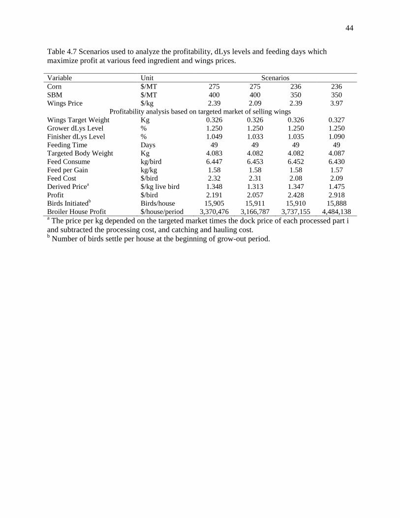
44
Table 4.7 Scenarios used to analyze the profitability, dLys levels and feeding days which maximize profit at various feed ingredient and wings prices. Variable Unit Scenarios Corn $/MT 275 275 236 236 SBM $/MT 400 400 350 350 Wings Price $/kg 2.39 2.09 2.39 3.97
Profitability analysis based on targeted market of selling wings Wings Target Weight Kg 0.326 0.326 0.326 0.327 Grower dLys Level % 1.250 1.250 1.250 1.250 Finisher dLys Level % 1.049 1.033 1.035 1.090 Feeding Time Days 49 49 49 49 Targeted Body Weight Kg 4.083 4.082 4.082 4.087 Feed Consume kg/bird 6.447 6.453 6.452 6.430 Feed per Gain kg/kg 1.58 1.58 1.58 1.57 Feed Cost $/bird 2.32 2.31 2.08 2.09 Derived Pricea $/kg live bird 1.348 1.313 1.347 1.475 Profit $/bird 2.191 2.057 2.428 2.918 Birds Initiatedb Birds/house 15,905 15,911 15,910 15,888 Broiler House Profit $/house/period 3,370,476 3,166,787 3,737,155 4,484,138 a The price per kg depended on the targeted market times the dock price of each processed part i and subtracted the processing cost, and catching and hauling cost. b Number of birds settle per house at the beginning of grow-out period.

45
Table 4.8 Composition of the diets during grower and finisher phases which maximize profit for carcass market where corn, SBM and carcass prices were $275 and 400 per MT, and $1.87 per kg, respectively. Ingredients Grower Diet Finisher Diet Corn 69.47 76.79 Soybean Meal 22.63 16.40 Meat & Bone Meal 3.00 3.00 Poultry Fat 2.19 1.09 L-LysineHCl 0.17 0.16 DL-Methionine 0.27 0.19 L-Threonine 0.07 0.05 Limestone 1.05 1.06 Defluorinated P 0.18 0.23 Salt 0.42 0.27 UGA Vitamin PMX 0.25 0.25 UGA Mineral PMX 0.08 0.08 Choline Chloride 0.05 0.07 S-Carb 0.00 0.19 Copper Sulfate 0.04 0.04 Quantum 2,500 0.02 0.02 BMD-50 0.05 0.05 Coban 90 0.06 0.06 Total 100.00 100.00 Feed cost, $/ MT 367.1 346.8

46
Table 4.9 Nutrient composition of the diets during grower and finisher phases which maximize profit for the carcass market where corn, SBM and carcass prices were $275 and 400 per MT, and $1.87 per kg, respectively. Composition Grower Diet Finisher Diet Nutrients (% and Ratios) Crude Protein, % 17.45 14.86 ME Mcal / kg 3.16 3.16 Digestible Lys, % 0.89 0.73 Dig Met / Dig Lys 54 52 Dig M+C / Dig Lys 77 77 Dig Thr / Dig Lys 67 67 Dig Trp / Dig Lys 19 19 Dig Ile / Dig Lys 68 68 Dig Val / Dig Lys 79 81 Dig Arg / Dig Lys 116 117 Tot Gly / Dig Lys 93 100 Calcium, % 0.93 0.93 Avaliable P., % 0.46 0.46 Ca / Available P 2.00 2.00 Sodium, % 0.22 0.22 Digestible Amino Acids (%) Lysine 0.89 0.73 Methionine 0.48 0.38 Met + Cys 0.68 0.56 Threonine 0.59 0.49 Tryptophan 0.17 0.14 Isoleucine 0.60 0.49 Valine 0.70 0.59 Arginine 1.03 0.85 Leucine 1.27 1.12 Histidine 0.37 0.31 Alanine 0.77 0.68 Glutamic Acid 2.52 2.11 Aspartic Acid 1.36 1.10 Phenylalanine 0.73 0.61 Proline 0.91 0.81 Serine 0.70 0.59 Tyrosine 0.33 0.28 Total Glycine 0.71 0.61 Dig. Essential Amino Acids (DEAA) 6.83 5.69 Dig. Non-essential Amino Acids (DNEAA) 7.50 6.37 Sum of the Dig. AA (DAA) 14.33 12.07 DEAA / DAA 47.65 47.17 DNEAA / DAA 52.35 52.83 DAA / CP 82.15 81.22

47
Table 4.10 Summary of the scenarios changed to the dLys levels and feeding days which maximize profit at various feed ingredient and cut-up part prices.
Variables (y) Unit Profitability analysis based on targeted market of selling cut-up parts Carcass Breast meat Tenderloin Leg quarters Wings
Cut-Up Part Target Weight Kg
Grower dLys Level %
Finisher dLys Level %
Feeding Time Days
Targeted Body Weight Kg
Feed Consume Kg/bird
Feed Cost $/bird
Profit $/bird
is the price of cut-up part; is the price of feed ingredients.

48
Table 4.11 Descriptive statistics of the corn and soybean meal (SBM) prices and their spread (SBM minus corn prices) between low volatile period (January 2000 to December 2005) and high volatile period (January 2006 to April 2011).
Descriptive Statistics Corn SBM Spread $/MT $/MT $/MT
Descriptive Statistics between January 2000 and December 2005 Mean 98.76b 204.90b 106.14b
Variance 135.52 1691.60 1063.54 Minimum 75.06 165.45 74.19 Maximum 133.39 343.71 210.32 Skewness 0.79 1.92 1.76 Kurtosis 1.09 3.25 2.62 Standard Deviation 11.64 41.13 32.61 N 72 72 72
Descriptive Statistics between January 2006 and April 2011 Mean 179.43a 309.35a 129.92a
Variance 2539.46 5918.71 2430.86 Minimum 102.70 175.91 45.03 Maximum 318.45 452.19 262.95 Skewness 0.85 -0.21 0.36 Kurtosis 0.31 -1.05 0.02 Standard Deviation 50.39 76.93 49.30 N 64 64 64 1 The difference between feeding the dLys levels that maximized profit (Maximum profit) and the dLys levels that recommended by the breeder (Conventional profit). Means in a column with different letters (LSD multiple range test) differ significantly (P < 0.05).

49
Table 4.12 Descriptive statistics of dLys levels that maximized profit during grower and finisher phases, revenue, total cost, maximum profit, conventional profit and cost of making wrong decision between low volatile period (January 2000 to December 2005) and high volatile period (January 2006 to April 2011).
Descriptive Statistics
Grower dLys level
Finisher dLys level Revenue Total cost Maximum profit
Conventional profit
Cost of making wrong decision1
% % Cent/bird Cent/bird Cent/bird Cent/bird Cent/bird Descriptive Statistics between January 2000 and December 2005
Mean 1.25a 0.78 571.08a 211.40b 359.68a 356.93a 2.75
Variance 0.02 0.004 28.39 81.57 189.08 224.85 −35.77 Minimum 0.78 0.71 552.25 194.97 315.79 307.10 8.69 Maximum 1.30 0.95 575.34 236.46 378.72 376.41 2.31 Skewness -2.52 0.63 -2.43 0.86 -1.61 -1.79
Kurtosis 5.06 -0.18 4.92 0.60 2.41 2.99 Standard Deviation 0.13 0.06 5.33 9.03 13.75 15.00 N 72 72 72 72 72 72 Descriptive Statistics between January 2006 and April 2011
Mean 1.09b 0.77 565.27b 263.20a 302.07b 299.14b 2.93
Variance 0.03 0.01 56.82 1009.12 1316.84 1342.07 −25.23 Minimum 0.77 0.71 551.75 213.21 222.99 222.69 0.29 Maximum 1.30 1.05 576.69 349.35 359.63 357.55 2.07 Skewness -0.06 1.74 0.0002 0.64 -0.36 -0.31
Kurtosis -1.40 2.00 -1.27 0.12 -0.42 -0.50 Standard Deviation 0.18 0.10 7.54 31.77 36.29 36.63 N 64 64 64 64 64 64 1 The difference between feeding the dLys levels that maximized profit (Maximum profit) and the dLys levels recommended by the
breeder (Conventional profit). Means in a column with different letters (LSD multiple range test) differ significantly (P < 0.05).
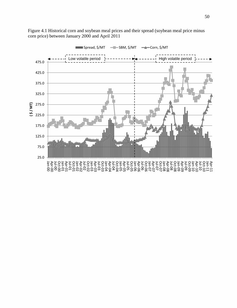
50
Figure 4.1 Historical corn and soybean meal prices and their spread (soybean meal price minus corn price) between January 2000 and April 2011
25.0
75.0
125.0
175.0
225.0
275.0
325.0
375.0
425.0
475.0
Jan-0
0A
pr-0
0Ju
l-00
Oct-0
0Jan
-01
Ap
r-01
Jul-0
1O
ct-01
Jan-0
2A
pr-0
2Ju
l-02
Oct-0
2Jan
-03
Ap
r-03
Jul-0
3O
ct-03
Jan-0
4A
pr-0
4Ju
l-04
Oct-0
4Jan
-05
Ap
r-05
Jul-0
5O
ct-05
Jan-0
6A
pr-0
6Ju
l-06
Oct-0
6Jan
-07
Ap
r-07
Jul-0
7O
ct-07
Jan-0
8A
pr-0
8Ju
l-08
Oct-0
8Jan
-09
Ap
r-09
Jul-0
9O
ct-09
Jan-1
0A
pr-1
0Ju
l-10
Oct-1
0Jan
-11
Ap
r-11
( $
/ M
T)
Spread, $/MT SBM, $/MT Corn, $/MT
Low volatile period High volatile period

51
Figure 4.2 Probability distributions of maximum profit conditions during low (January 2000 to December 2005) and high (January 2006 to April 2011) volatile periods
0.00
0.10
0.20
0.30
0.40
0.50
0.60
Maximum Profit, cent per bird
Prob
abili
tyD
ensi
ty
Low volatile period
High volatile period

52
CHAPTER 7
CONCLUSIONS
The objective of this research was to demonstrate that the broiler production decision,
based on the targeted market for selling whole carcass or cut-up parts, can be evaluated using
broiler growth performance information and a profit function. Nonlinear models of production
functions, using broiler growth performance information, were used in the profit function to
evaluate a profit-maximization condition that operated under Microsoft Excel spreadsheet. The
spreadsheets make the analysis accessible to chicken producers and integrators. The profit model
can determine the optimum conditions where a producer utilizes its production, inputs, and
processing plant to obtain the maximum profit. This research showed that growth responses can
vary depending on the maximum profit of feeding the formulated diet to broilers under various
feed ingredient and broiler market prices. At constant output prices, increasing input costs
decreases the size of bird that maximizes profits. Similarly, at constant input costs, increasing
output prices increases the size of bird that maximizes profits. The marginal product of input
(feed consumption) is the change in output (liveweight) as the change in feed consumption goes
to zero. To maximize profit, the marginal product of feed consumption must be equal to the
price of the feed consumed divided by the liveweight price. Profitability can be improved when
revenue and costs are both considered in the formulation of broiler diets. Broiler growth and feed
intake are two key components in determining the profit, which are not considered in traditional
least-cost feed formulation.

53
In this research, an experiment was conducted to obtain the data necessary to evaluate the
broiler production responses (body weight and feed intake) of dietary balanced protein (based on
digestible lysine (dLys) level). The broiler diets used in this research were based on corn,
soybean meal, meat and bone meal and synthetic amino acids to assure the dietary protein was
balanced. The data collected from the experiment were used to estimate the production functions.
Data used for economic analysis were obtained from a confidential survey conducted with a
poultry company and the Georgia Department of Agriculture. The information contained prices
of ingredients, production costs and targeted market prices.
The Cobb-Douglas (CD) production functions were adopted. The coefficients of the CD
can be used to explain the elasticity among the variables. Results indicated that body weight of
broilers increased about 0.87 percent for every one percent increased in feed intake. Analysis
showed that broiler fed with one percent higher in dLys increased broilers’ body weight by 0.06
and 0.08 percents during grower and finisher phases, respectively. Feed intake was analyzed as a
function of time (number of grow-out day) and dLys levels during grower and finisher phases.
Results showed that feed intake increased about 1.74 percent for every one percent
increase in the number of grow-out days. Analysis showed that broilers fed with one percent
higher digestible lysine level (dLys) increased feed consumption by 0.01 during grower phase
while decreasing feed consumption by 0.07 percent during finisher phases. Carcass and cut-up
part weights were determined as functions of live body weight and dLys levels during grower
and finisher phases. Results showed that carcass and cut-up part weights, except leg quarters and
rest of carcass, increased as live body weight and the level of dLys in the diets increased. Thus,
carcass and cut-up part weight can be improved by feeding higher level of dLys. This suggested
that feeding broilers at higher dLys levels improved broiler market value.

54
The estimated production functions were used in the profit maximization analysis of the
programming model. The optimum feeding levels of dLys were determined based on input costs,
output prices and other fixed and variable costs of broiler production. The optimum broiler
weight, number of grow-out day, feed consumption and feed formulation that provided the
maximum profit was estimated. The profit function was defined as average price of a broiler
( ) times live body weight (BW), minus total cost (TC). The TC is the calculation of least-
cost feed ( ) plus feed delivery cost (DEL) times feed consumed and interest (future cost
accounted for feed consumption at d); plus the sum of grower cost (GRO) and field DOA and
condemnation cost (FDOA) times broiler weight and interest (future value of chicken at d); plus
fixed cost (TFC) such as chick cost, vaccination, supervising, and miscellaneous costs. The
interest cost (I) was the calculation of
, where d is feeding days and i is the annual
interest rate of the grower.
The programming model provided alternative options on targeted market of broilers
either selling a whole carcass or cut-up parts. Moreover, the model also formulated the diets that
maximized profit of broiler production. For all the scenarios studied here, the most profitable
strategy of a broiler company was to target the market of selling cut-up parts. At constant output
prices (broiler market prices), increasing input costs (feed cost) decreases the size of bird that
maximizes profits. Likewise, at constant input costs, increasing output prices increases the size
of bird that maximizes profits. These results agreed with previous published article by Pesti et al.
(2009a and 2009b).

55
REFERENCES
Allison, J.R., and D. Baird. 1974. "Least-cost livestock production rations." Southern journal of
agricultural economics 6(2):41-45.
Agri Stats, Inc. 2010. Monthly Live Production. 6510 Mutual Dr. Fort Wayne, IN 46825.
Ajinomoto Heartland LLC. 2009. True Digestibility of Essential Amino Acids for Poultry.
Ajinomoto Heartland LLC, Chicago, IL.
Aviagen. 2007. Ross 708 broiler performance objectives. Aviagen, Newbridge, Scotland.
Baker, D., A. Batal, T. Parr, N. Augspurger, and C. Parsons. 2002. "Ideal ratio (relative to lysine)
of tryptophan, threonine, isoleucine, and valine for chicks during the second and third
weeks posthatch." Poultry science 81(4):485-494.
Beattie, B.R., and C.R. Taylor. 1985. The Economics of Production: John Wiley & Sons, Inc.
Black, J.R., and J. Hlubik. 1980. "Basics of Computerized Linear Programs for Ration
Formulation." Journal of Dairy Science 63(8):1366-1378.
Brown, W.G., and G. Arscott. 1960. "Animal production functions and optimum ration
specifications." Journal of Farm Economics 42(1):69-78.
Cerrate, S., and P. Waldroup. 2009a. "Maximum Profit Feed Formulation of Broilers: 1.
Development of a Feeding Program Model to Predict Profitability Using non Linear
Programming." International Journal of Poultry Science 8(3):205-215.
Cerrate, S., and P. Waldroup. 2009b. "Maximum Profit Feed Formulation of Broilers: 2.
Comparison among Different Nutritional Models." International Journal of Poultry
Science 8(3):216-228.

56
Coelli, T. 2005. An introduction to efficiency and productivity analysis: Springer Verlag.
Corzo, A. (2008) Maximizing production efficiency by a better understanding of the 4th limiting
amino acid in broiler formulation. Timonium, Maryland, pp. 76-81.
Costa, E.F., B.R. Miller, J.E. Houston, and G.M. Pesti. 2001. "Production and profitability
responses to alternative protein sources and levels in broiler rations." Journal of
Agricultural and Applied Economics 33(3):567-582.
D'Mello, J. 2003. Amino acids in animal nutrition. CABI Publishing, Cambridge, MA.
Darmani Kuhi, H., E. Kebreab, S. Lopez, and J. France. 2009. "Application of the law of
diminishing returns to estimate maintenance requirement for amino acids and their
efficiency of utilization for accretion in young chicks." The Journal of Agricultural
Science 147(04):383-390.
Douglas, P.H. 1976. "The Cobb-Douglas Production Function Once Again: Its History, Its
Testing, and Some New Empirical Values." The Journal of Political Economy 84(5):903-
916.
Dozier III, W., R. Gordon, J. Anderson, M. Kidd, A. Corzo, and S. Branton. 2006.
"Growth, meat yield, and economic responses of broilers provided three-and four-phase
schedules formulated to moderate and high nutrient density during a fifty-six-day
production period." The Journal of Applied Poultry Research 15(2):312.
Eits, R., R. Kwakkel, M. Verstegen, and L. Hartog. 2005a. "Dietary balanced protein in broiler
chickens. 1. A flexible and practical tool to predict dose–response curves." British
Poultry Science 46(3):300-309.

57
Eits, R., G. Giesen, R. Kwakkel, M. Verstegen, and L. Den Hartog. 2005b. "Dietary
balanced protein in broiler chickens. 2. An economic analysis." British Poultry Science
46(3):310-317.
Frontline Systems, Inc. 1999. Solver User’s Guide. Incline Village, NV.
Emmert, J., and D. Baker. 1997. "Use of the ideal protein concept for precision formulation of
amino acid levels in broiler diets." The Journal of Applied Poultry Research 6(4):462-
470.
Frontline Systems, Inc. 1999. Solver User’s Guide. Incline Village, NV.
Garrett, H., and C. Grisham. 2007. Biochemistry. Fort Worth: Thomson Learning.
Georgia Department of Agriculture. 19 Martin Luther King, Jr. Dr., S.W. Atlanta,
Georgia 30334. http://agr.georgia.gov/portal/site.
Gonzalez-Alcorta, M.J., J.H. Dorfman, and G.M. Pesti. 1994. "Maximizing profit in broiler
production as prices change: A simple approximation with practical value." Agribusiness
10(5):389-399.
Guevara, V. 2004. "Use of nonlinear programming to optimize performance response to energy
density in broiler feed formulation." Poultry science 83(2):147-151.
Heady, E.O. 1957. "An econometric investigation of the technology of agricultural
production functions." Econometrica: Journal of the Econometric Society 25(2):249-
268.
Henderson, J.M., and R.E. Quandt. 1980. Microeconomic Theory: A Mathematical Approach.
3rd ed: McGraw-Hill Book Company.
Hyman, D.N. 1989. Modern Micoreconomics: Analysis and Applications. 2nd ed. North
Carolina: Times Mirror /Mosby College Publishing.

58
Kennedy, J., B. Rofe, I. Greig, and J. Hardaker. 1976. "Optimal feeding policies for broiler
production: an application of dynamic programming." Australian Journal of Agricultural
Economics 20(01):19-32.
Kidd, M., and L. Hackenhaar. 2006. "Dietary threonine for broilers: dietary interactions and feed
additive supplement use." CAB Reviews: Perspectives in Agriculture, Veterinary Science,
Nutrition and Natural Resources.
Kmenta, J. 1967. "On Estimation of the CES Production Function." International Economic
Review 8(2):180-189.
Lemme, A., C. Kemp, E. Fleming, and C. Fisher. 2008. Impact of increasing levels of balanced
protein on biological and economic parameters of two different commercial broiler lines:
Ross 308 and Ross 708. Brisbane, Australia.
Mack, S., D. Bercovici, G. De Groote, B. Leclercq, M. Lippens, M. Pack, J. Schutte, and S. Van
Cauwenberghe. 1999. "Ideal amino acid profile and dietary lysine specification for
broiler chickens of 20 to 40 days of age." British Poultry Science 40(2):257-265.
Mansfield, E. 1988. Microeconomics: Theory and Applications. 6th ed: W.W.
Norton&Company, Inc.
Mendenhall, W., Sincich, T., 2003. A second course in statistics: Regression analysis. Pearson
Education, Inc. NC, USA.
Miller, B.R., R.A. Arraes, and G.M. Pesti. 1986. "Formulation of broiler finishing rations
by quadratic programming." Southern journal of agricultural economics 18(01):141-
150.
Mills, G. 1984. Optimisation in Economic Analysis. 1st ed. UK: George Allen & Unwin
(Publishers) Ltd.

59
Mundi, I. (2009) Historical Commodity Prices, Index Mundi.
http://www.indexmundi.com/commodities/ .
Pesti, G., R. Arraes, and B. Miller. 1986. "Use of the quadratic growth response to dietary
protein and energy concentrations in least-cost feed formulation." Poultry science
65:1040-1051.
Pesti, G.M., N. Sriperm, and M.E. Wetzstein. "Optimizing Broiler Profitability during Difficult
Times-Part One: Impact of liveweight and carcass weight on optimizing profit."
Feedstuffs, February 23, 2009a, pp. 16-17.
Pesti, G.M., N. Sriperm, and M.E. Wetzstein. "Optimizing Broiler Profitability during Difficult
Times-Part two:Maximizing Profitability with Optimal Nutrient Density." Feedstuffs,
May 25, 2009b, pp. 22-25.
Pesti, G., D. Vedenov, J. Cason, and L. Billard. 2009c. "A comparison of methods to
estimate nutritional requirements from experimental data." British Poultry Science
50(1):16-32.
Romero, L., M. Zuidhof, R. Renema, F. Robinson, and A. Naeima. 2009. "Nonlinear mixed
models to study metabolizable energy utilization in broiler breeder hens." Poultry science
88(6):1310-1320.
SAS User’s Guide. 2004. Version 9.1 ed. SAS Inst. Inc., Cary, NC.
Sriperm, N., and G.M. Pesti. 2011. "Response Surface Analysis of Dietary Balanced Protein
responses during grower and finisher phases of Ross 708 male broilers." Dissertation,
University of Georgia.
Sterling, K., D. Vedenov, G. Pesti, and R. Bakalli. 2005. "Economically optimal dietary crude
protein and lysine levels for starting broiler chicks." Poultry science 84(1):29-36.

60
Talpaz, H., S. Hurwitz, J.R. de la Torre, and P.J.H. Sharpe. 1988. "Economic optimization of a
growth trajectory for broilers." American Journal of Agricultural Economics 70(2):382-
390.
Timothy, J.C., D.S.P. Rao, C.J. O'Donnell, and G.E. Battese. 2005. An introduction to
eficiency and productivity analysis. 2nd ed. Queensland: Springer Science and
Business Media, Inc.
Tesseraud, S., R. Peresson, J. Lopes, and A. Chagneau. 1996. "Dietary lysine deficiency greatly
affects muscle and liver protein turnover in growing chickens." British Journal of
Nutrition 75(6):853-865.
Walters, A. 1963. "Production and cost functions: An econometric survey." Econometrica:
Journal of the Econometric Society 31(1):1-66.
Wijtten, P., A. Lemme, and D. Langhout. 2004. "Effects of different dietary ideal protein levels
on male and female broiler performance during different phases of life: single phase
effects, carryover effects, and interactions between phases." Poultry science 83(12):2005-
2015.
Zellner, A., J. Kmenta, and J. Dreze. 1966. "Specification and estimation of Cobb-
Douglas production function models." Econometrica: Journal of the Econometric Society
34(4):784-795.
Zuidhof, M.J. (2009) Nonlinear Effects of Diet on Broiler Production. Rogers, Arkansas.

61
APPENDIX A
Table A 1.1 Production costs used in the profit maximization analysis
Variables Abbreviation Values Unit
Interest Cost I 1.01 %
Feed Cost rFC 29.85 Cent/lb
Chick Costs TFC 29.79 Cent/chick
Vaccination, Supervising, Miscellaneous TFC 1.61 Cent/chick
Grower Costs GRO 6.06 Cent/lb
Milling and Delivery Cost DEL 1.50 Cent/lb
DOA and Field Condemnation Cost FDOA 0.33 Cent/lb
Cost of Catching and Hauling CH 1.45 Cent/lb
Processing Cost PC
Step 1: Including all fixed overhead
7.50 Cent/lb
Step 2: Cutting and Packaging
9.75 Cent/lb
Total Cost
386.07 Cents / bird

62
APPENDIX B
Table B 1.1 Corn and soybean meal prices and their spread (soybean meal minus corn)
Month
/ Year
Corn,
$/MT
SBM,
$/MT
Spread,
$/MT
Jan-00 92.95 172.43 79.48 Feb-00 95.08 180.47 85.39 Mar-00 95.17 185.63 90.46 Apr-00 95.54 187.86 92.32 May-00 95.53 200.98 105.45 Jun-00 84.04 191.49 107.45 Jul-00 75.06 175.93 100.87
Aug-00 75.24 171.07 95.83 Sep-00 80.15 188.03 107.88 Oct-00 84.71 186.00 101.29 Nov-00 88.94 194.33 105.39 Dec-00 96.22 211.81 115.59 Jan-01 94.30 197.59 103.29 Feb-01 92.38 178.71 86.33 Mar-01 91.01 169.52 78.51 Apr-01 87.55 169.02 81.47 May-01 85.08 178.07 92.99 Jun-01 83.16 185.04 101.88 Jul-01 90.75 194.23 103.48
Aug-01 92.88 189.10 96.22 Sep-01 89.74 183.94 94.20 Oct-01 86.27 177.63 91.36 Nov-01 89.88 177.99 88.11 Dec-01 92.31 166.50 74.19 Jan-02 91.97 169.58 77.61 Feb-02 90.73 165.45 74.72 Mar-02 89.86 174.29 84.43 Apr-02 87.11 175.93 88.82 May-02 90.33 179.90 89.57 Jun-02 93.17 185.83 92.66 Jul-02 99.70 204.24 104.54
Aug-02 109.89 201.12 91.23 Sep-02 113.94 200.25 86.31 Oct-02 109.65 185.35 75.70 Nov-02 108.65 183.88 75.23 Dec-02 107.01 181.98 74.97 Jan-03 105.75 184.87 79.12 Feb-03 106.04 192.42 86.38 Mar-03 105.06 191.36 86.30 Apr-03 105.25 200.26 95.01
Month
/ Year
Corn,
$/MT
SBM,
$/MT
Spread,
$/MT
May-03 107.82 214.18 106.36 Jun-03 106.99 210.61 103.62 Jul-03 97.61 200.44 102.83
Aug-03 100.31 199.30 98.99 Sep-03 103.22 218.14 114.92 Oct-03 104.17 245.71 141.54 Nov-03 108.03 262.96 154.93 Dec-03 111.98 255.64 143.66 Jan-04 115.09 278.48 163.39 Feb-04 122.91 286.39 163.48 Mar-04 128.43 331.41 202.98 Apr-04 133.39 343.71 210.32 May-04 129.30 331.65 202.35 Jun-04 123.23 311.68 188.45 Jul-04 104.48 291.01 186.53
Aug-04 104.04 212.15 108.11 Sep-04 97.76 182.69 84.93 Oct-04 93.37 171.44 78.07 Nov-04 93.75 170.13 76.38 Dec-04 95.59 175.72 80.13 Jan-05 95.98 175.18 79.20 Feb-05 94.36 178.55 84.19 Mar-05 99.94 207.64 107.70 Apr-05 96.39 210.27 113.88 May-05 95.27 218.01 122.74 Jun-05 97.56 241.22 143.66 Jul-05 105.60 238.80 133.20
Aug-05 98.64 217.60 118.96 Sep-05 96.99 193.57 96.58 Oct-05 101.50 186.58 85.08 Nov-05 95.97 192.15 96.18 Dec-05 102.66 209.58 106.92 Jan-06 102.70 201.96 99.26 Feb-06 106.92 198.43 91.51 Mar-06 104.89 192.43 87.54 Apr-06 107.82 190.55 82.73 May-06 110.57 193.25 82.68 Jun-06 109.55 196.26 86.71 Jul-06 114.24 187.27 73.03
Aug-06 115.21 175.91 60.70

63
Month
/ Year
Corn,
$/MT
SBM,
$/MT
Spread,
$/MT
Sep-06 120.26 177.59 57.33 Oct-06 142.17 194.12 51.95 Nov-06 164.08 214.23 50.15 Dec-06 160.66 205.69 45.03 Jan-07 165.10 221.79 56.69 Feb-07 177.35 244.10 66.75 Mar-07 169.52 239.53 70.01 Apr-07 152.58 221.75 69.17 May-07 156.44 227.67 71.23 Jun-07 164.50 249.16 84.66 Jul-07 147.13 252.57 105.44
Aug-07 151.01 251.83 100.82 Sep-07 160.05 288.78 128.73 Oct-07 164.09 300.43 136.34 Nov-07 171.06 315.25 144.19 Dec-07 180.25 351.22 170.97 Jan-08 206.53 376.33 169.80 Feb-08 219.95 396.71 176.76 Mar-08 233.85 379.70 145.85 Apr-08 246.67 375.32 128.65 May-08 243.46 369.37 125.91 Jun-08 287.11 436.91 149.80 Jul-08 266.94 452.19 185.25
Aug-08 235.16 388.40 153.24 Sep-08 233.91 363.78 129.87 Oct-08 182.96 290.84 107.88 Nov-08 164.27 292.76 128.49 Dec-08 158.16 292.94 134.78 Jan-09 173.24 338.50 165.26 Feb-09 163.13 320.89 157.76 Mar-09 164.52 315.37 150.85 Apr-09 168.72 349.57 180.85 May-09 180.31 408.05 227.74 Jun-09 178.83 441.78 262.95 Jul-09 151.76 385.85 234.09
Aug-09 152.01 397.30 245.29 Sep-09 150.57 342.18 191.61 Oct-09 167.22 328.54 161.32 Nov-09 171.61 337.63 166.02 Dec-09 164.58 345.58 181.00 Jan-10 167.21 325.85 158.64 Feb-10 161.63 303.66 142.03 Mar-10 159.01 292.60 133.59 Apr-10 157.66 308.05 150.39 May-10 163.77 305.74 141.97 Jun-10 152.87 314.32 161.45 Jul-10 163.92 335.09 171.17
Aug-10 175.60 339.14 163.54
Month
/ Year
Corn,
$/MT
SBM,
$/MT
Spread,
$/MT
Sep-10 205.84 334.06 128.22 Oct-10 235.70 353.75 118.05 Nov-10 238.24 376.04 137.80 Dec-10 250.63 387.51 136.88 Jan-11 265.29 412.07 146.78 Feb-11 293.40 410.16 116.76 Mar-11 290.43 393.93 103.50 Apr-11 318.45 388.22 69.77