Optimal Bandwidth Monitoring - University of...

Optimal Bandwidth Monitoring

© Y.Yu, I.Cheng and A.BasuDepartment of Computing Science

U. of Alberta

© Y.Yu, I.Cheng and A.Basu, UofA 2

Outline

� Introduction – The problem and objectives� The Bandwidth Estimation Algorithm� Simulation Results� Experiments on Real Networks� Conclusion


The Quest of QoS

What is Quality of Service (QoS)?

� “…Quality of Service is the set of quantitative and qualitative characteristics of a distributed multimedia system necessary to achieve the required functionality of an application…”

� QoS Parameters:� Lower Layer: Bandwidth, end-to-end delay� Higher Layer: Image/video resolution, compression

scheme, subjective image/sound quality


Resource Reservation

� Solution #1: Resource reSerVation Protocol (RSVP)� Service class beyond “best-effort”

� Flow specification� Admission control� Packet Scheduling

� Problem

� Require replacement of existing routers

� Introduce significantly heavier computation burden on routers


Content Adaptation

� Solution #2: Network-aware Application� Do not rely on underlying network to provide

guaranteed quality� Actively Monitors network performance and adapt

multimedia accordingly� Provide trade-off between QoS parameters for

certain application. E.g. Distant Education, virtual museum.


1. QoS Parameters

2. Trade-off Criteria

3. Fetch Content


Architecture

-connection handling-request processing

Request receptionApplication LayerApplication Layer

Adaptation LayerAdaptation Layer

-monitor/poll bandwidth

-determine object size

transform requested object to target size

deliver object To client

Monitor Prepare Transmit

Lower LayerLower Layer

Object delivery across network

feedback from network


The Bandwidth Monitoring Problem� Obviously, accurate bandwidth estimation is of critical

importancePrevious solution:

� Maintain session between server and client� Periodically send testing packets to client to obtain

bandwidth samples� Using some kind of average of sample bandwidth as

bandwidth estimation Drawbacks:

� Bandwidth sample may not be most updated� Waste bandwidth on monitoring when no actual

transmission is requested


Objectives

� To design a new algorithm of bandwidth estimation for network-aware applications

Assumptions:� One client and one or more server(s) need to perform a one-

off transmission of a multimedia object� QoS parameter: end user specified time limit� First fraction of the time limit is used for bandwidth testingTarget:� Guarantees the QoS parameter to a certain confidence level� Maximize the multimedia object transmitted


The Source of Bandwidth Variance

TCP Congestion Control� Design goal: detect and sustain the available

bandwidth on the network without creating congestion

� Typical Bandwidth pattern (TCP Vegas)


TCP Evolution�TCP is an ever-evolving protocol, with new mechanisms

continuously proposed and implemented

YesNoNoCongestion Detection/ Avoidance

YesYesNoFast Recovery

YesYesYesFast Retransmit

YesYesYesAdditive Increase/ Multiplicative Decrease

YesYesYesSlow Start

TCP VegasTCP Reno (BSD Network Release 2.0)

TCP Tahoe (BSD Network Release 1.0)


Related ResearchBandwidth Estimation in TCP layer:� Jacobson, base on size of congestion window, RTT.� Mathis, Padhye, base on factors like packet loss rate, packet

size, number of timeouts, and average duration of retransmission timeout.

Pros and Cons:� Accessible to micro-factors of TCP, yielding accurate

estimation.� Need frequent revision and re-evaluation as new mechanisms

are added to TCP version.� Not available to application programmers for the purpose of

developing network-aware applications.


Our Contribution

� A bandwidth estimation algorithm working on Application Layer.

� Based on statistical model, shielded from micro-factors of TCP.

� Easily integrated to network-aware applications by application programmers.


Outline

� Introduction – The problem and objectives� The Bandwidth Estimation Algorithm� Simulation Results� Experiments on Real Networks� Conclusion


Assumptions and Notations

� One server and one client need to make a one-time transmission of a multimedia object (server to client).

� User specified a time limit T on client. It’s expected that the transmission will finish within T by confidence level .

� The first fraction t of T will be used for bandwidth testing.� Bandwidth testing is performed by using time slices of equal

length . Each time slice has bandwidth sample � , bandwidth population� , bandwidth samples

α

st sii tCx /=

stTN /= NXXX ,...,, 21

sttn /= nxxx ,...,, 21


� , is the average of bandwidth samples.

� , is the variance of bandwidth samples.

� , is actual bandwidth we try to estimate.

Notations

Our Problem is:� First, given N, n, , , give an estimation of , so that

. � Second, determine optimal value of n, in order to maximize

. [Exercise: FIX ONE PROBLEM IN THE PROB. Expression]

x 2s µ( ) αµµ =<estP

( ) sest tnN ⋅−⋅µ

( )1

12

2

−−

= ∑ =

nxx

sn

i i

NXN

i i∑ == 1µ

nx

xn

i i∑ == 1


� is a continuous random variable following

“student-t” distribution.

Student-t Distribution

1−−⋅

−=

NnN

ns

xd µ


� Probability distribution � Safe bandwidth estimation

� t-distribution table ( values)

Safe Bandwidth Estimation

1−−⋅⋅+=

NnN

nsdxµ

( ) 1, −−⋅⋅−=

NnN

nsdx nest αµ

( )nd ,α

1.8121.3720.700n=10

2.0151.4760.727n=5

2.1321.5330.741n=4

2.3531.6380.765n=3

2.9201.8860.816n=2

6.3143.0781.000n=1

Alpha=0.95Alpha=0.90Alpha=0.75


� Expect Object Size� Important property of V(n):

Statistically (if we view random variable and s as constant),V(n) has a single maximum value. (Proof omitted)

� Intuition of the property:When n is too large, too much time is used for bandwidth testing, leaving little time for real object transmission;when n is too small, value is too large, leading to great margin of under-estimation of bandwidth.

Expected Object Size

( ) ( ) ( ) sest tnNnnV ⋅−⋅= µ

x

( )nd ,α


Single Server Optimal Bandwidth Testing

� The Algorithm:obtain samples ;

Calculate V(1) and V(2);

;

while (V(n)>V(n-1)) {

;

obtain sample ;

Calculate V(n);

}

return ; �

321 ,, xxx

2←n

1+← nn1+nx

estµ


Outline

�Introduction – The problem and objectives

�The Bandwidth Estimation Algorithm

�Simulation Results

�Experiments on Real Networks

�Conclusion


Goal of Simulation Experiments

� Verify the effectiveness of the algorithm on:� How well the confidence level on time limit is

met?� Does it find the optimal amount of bandwidth

testing?• Use the real object transmission time as a gauge to

measure the merit of algorithms• Comparing our algorithm with a straightforward

method of taking fixed number of bandwidth samples.


Simulator

Set parameter

Start Simulation

Result

Parameters:• , which represent the bandwidth characteristics of the channel.• N, total number of time slices• , the confidence level on time limit.

σµ ,

α


Simulation Process�Bandwidth testing

� A normal distributed random number is generated as the bandwidth of the time slice.� Our algorithm is used to determine whether bandwidth testing should continue and the expect object size V(n).

�Real Transmission� For each time slice a random number is generated again and usedto compute the byte count received in this slice.� The byte count is subtracted from the remaining object size. The transmission finishes when remaining size drop below zero.

�Results� Transmitted object size. Whether it finish within time limit. Real transmission time.


Continuous decrease method

� Although Statistically, V(n) has one maximum, it is actually serrated, with multiple local maximums.

� We use three continuous drop in V(n) as the termination condition.

� Results is not very good.

Serrated V(n) curve


Hotel 2

Hotel 1

done

Moving Average Method

� We keep the average of past four V(n) for each time slice. � The simulator terminates the bandwidth testing when there are

three continuous drop in this “moving average” of V(n).� Results is much better.

Results much better


Real Transmission Time, Fix Sampling

Experiment parameters: alpha=0.95, 500 total time slices. Bandwidth average 100kbps, standard deviation is {5, 10, 15, 20, 25, 30,35, 40, 45, 55, 60}.

Large sample numberssuffers because too muchtime used for BW testing.

Small sample numberssuffer because of largeUnder-estimation Margin.


Our Algorithm vs. Fix Sampling, 500 slices

Room information

20%

5%

4%7%


Experiment parameters: alpha=0.95, 100 total time slices.Bandwidth average 100kbps, standard deviation is {5, 10, 15, 20, 25, 30,35, 40, 45, 55, 60}.

Real Transmission Time, Fix Sampling 2


Our Algorithm vs. Fix Sampling, 100 slices

40%

25%


Time Limit Confidence Level Results

Time Limit Confidene Level Result (100 slices)

0

5

10

15

20

5 10 15 20Number of Fix Samples

Num

ber o

f Ove

rtim

eRu

n (o

ut o

f 200

)

DynamicSampling

FixSampling

Time Limit ConfidenceLevel Result(500slice)

02468

101214

10 20 30 40Number of Fix Samples

Num

ber o

f rtim

eR

un (o

ut o

f 200

)

DynamicSampling

FixSampling

7% 5.5%

� Each bar is average of all the bandwidth standard deviation.� Alpha has been 0.95 for all the experiments.� The number of runs exceeding time limit is around 5.5% and

7%.


Outline

�Introduction – The problem and objectives




�Conclusion


Purpose of experiments on real networks

� Verify assumption� We assume the first n samples are representative

of the entire bandwidth population

� Address practical issues� E.g.: selecting time slice size

� Check computation cost


Implementation

Parameter Setting

Start Simulation

Statistics

Bandwidth Samples


Transmission procedure

Client runs our algorithm to perform bandwidth testing, until the termination condition is met.

Client finishes receiving, records finish time, calculates and displays statistics of the transmission.

Client: creates a TCP connection to server, and sent a TEST command.Server: begin to send a stream of random bytes to client

Client tears down the TCP connection and makes a new one.Client sends a TRANSMIT command with parameter of target object size,

which equals to ( ) esttT µ⋅−

( ) esttT µ⋅−Server sends the object with size


Experiment Scenario 1: campus network

eva133.cs.ualberta.ca(129.128.4.181)

Campus Network

ipiatik.cs.ualberta.ca(129.128.25.208)


Experiment results

204Total No. of Exception in 100 runs

9.859.80Actual Total Time (s)

9.679.49Actual Transmission Time (s)

13611337Actual Object Size (KB)

140.8141.0Actual Bandwidth Avg (kbps)

138.5137.8Estimation (kbps)

8.657.71Sample Standard Error

140.6141.2Sample Average (kbps)

8.714.6Average No. of Sample

0.750.95Confidence Goal Parameters:Time limit: 10sTime slice: 0.02sResults are average of 100 runs.Controlled under-estimation

95-97% of time used for real transmission!

Time limit confidence level satisfactorily met.


Comparison with fix sampling

Our algorithm


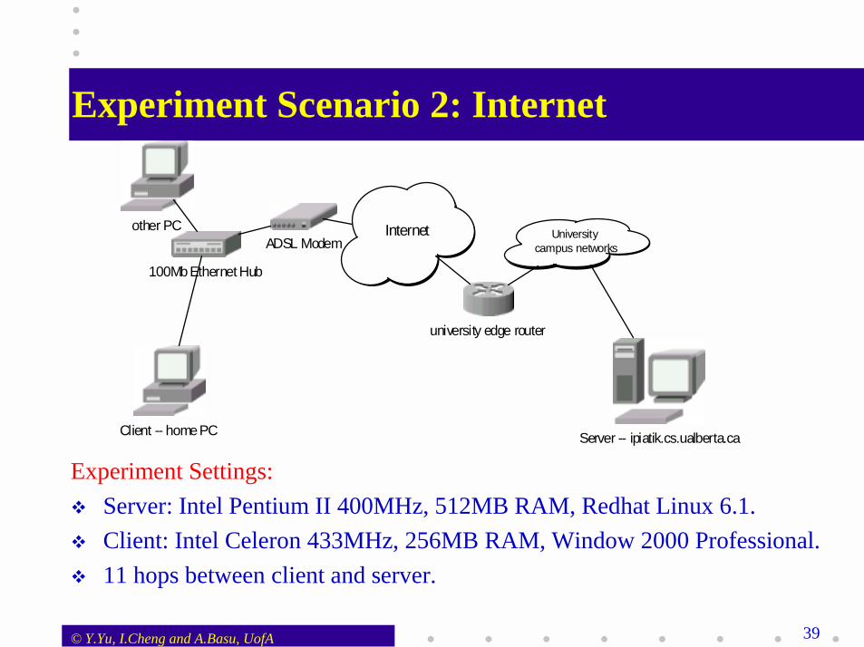
Experiment Scenario 2: Internet

Client -- home PC

100Mb Ethernet Hub

Internet

university edge router

University campus networks

Server -- ipiatik.cs.ualberta.ca

ADSL Modemother PC

Experiment Settings:� Server: Intel Pentium II 400MHz, 512MB RAM, Redhat Linux 6.1.� Client: Intel Celeron 433MHz, 256MB RAM, Window 2000 Professional. � 11 hops between client and server.


Experiment results




13941345Actual Object Size (KB)






0.750.95Confidence Goal Parameters:Time limit: 10sTime slice: 0.05sResults are average of 100 runs.

In turn, less time for real transmission.

Time limit confidence level still within range.

Relatively larger standard error in samples.


Different time slice size

Time slice = 0.02s Time slice = 0.05s

Time slice = 0.10s


Different time slice size

9.61

8.60

134K

156.4

144.8

24.3

156.0

14.0

200

0.05 0.100.02Time Slice Size (s)

100500Total time slice number






130K129KActual Object Size (KB)



No. of sample decrease, but sampling time increase!

6% different in estimation

3.5% different in object size.

There is a best slice size which maximize object size. However, the difference between using different slice sizes is relatively small.


Experiment Scenario 3: Internet with wireless link

Home PC (Router)

100M b Ethernet Hub

Internet

university edge router

University campus networks

Server -- ipiatik.cs.ualber ta.ca

AD SL M odem

other PC

C lient laptop

Experiment Settings:� Server: Intel Pentium II 400MHz, 512MB RAM, Redhat Linux 6.1.� Client: Intel Pentium MMX 233MHz laptop, 64MB RAM, Window 98. � 12 hops between client and server.


Experiment results10010Wireless link distance (feet)




90K126KActual Object Size (KB)






100100Total Time Slices NumberResults at different distance.

Alpha=0.95 in both cases.

Results similar with wired link.

Lower bandwidth

Larger variance

Low time limit utilization

More exception runs


Experiment results summary

� The assumption that bandwidth samples represent the entire bandwidth population is reasonable.

� Slice sizes within a relatively wide range all perform quite well.

� The algorithm runs smoothly on 233MHz laptop with Java implementation. The computation requirement is not high. The algorithm should be suitable to run on handheld devices.


Outline

�Introduction – The problem and thesis objective



�Extension of the Algorithm to Multi-server Scenario


�Conclusion

Optimal Bandwidth Monitoring - University of...

Documents

Transcript of Optimal Bandwidth Monitoring - University of...