Optimal active portfolio management and relative performance drivers ... · Optimal active...

BIS Papers No 58 187

Optimal active portfolio management and relative performance drivers: theory and evidence

Roberto Violi1

This paper addresses the optimal active versus passive portfolio mix in a straightforward extension of the Treynor and Black (T-B) classic model. Such a model allows fund managers to select the mix of active and passive portfolio that maximizes the (active) Sharpe ratio performance indicator. The T-B model, here adapted and made operational as a tool for performance measurement, enables one to identify the sources of fund management performance (selectivity vs market-timing). In addition, the combination of active and passive risk exposures is estimated and fund manager choice is tested against the hypothesis of optimal (active) portfolio design.

The extended T-B model is applied to a sample of US dollar reserve management portfolios – owned by the ECB and managed by NCBs – invested in high-grade dollar denominated bonds. The best fund managers show statistically significant outperformance against the ECB-given benchmark. By far, market timing is the main driver. Positive (and statistically significant) selectivity appears to be very modest and relatively rare across fund managers. These results are not very surprising, in that low credit risk and highly liquid securities dominate portfolio selection, thus limiting the sources of profitable bond-picking activity. As far as the risk-return profile of the active portfolio is concerned, it appears that some of the best fund managers’ outperformance is realised by shorting the active portfolio (with respect to the benchmark composition). Thus, portfolios that would be inefficient (eg negative excess return) if held long can be turned into positive-alpha yielding portfolios if shorted. The ability to select long-vs-short active portfolio can be seen as an additional source of fund manager’s outperformance, beyond the skill in anticipating the return of the benchmark portfolio (market-timing contribution).

The estimated measure of fund managers’ risk aversion turns out to be relatively high. This seems to be consistent with the fairly conservative risk-return profile of the benchmark portfolio. A relative measure of risk exposure (conditional Relative VaR) averaged across fund managers turns out to be in line with the actual risk budget limit assigned by the ECB. However, a fair amount of heterogeneity across fund managers is also found to be present. This is likely to signal a less-than-efficient use of their risk-budget by the fund managers – eg a deviation from the optimal level of relative risk accounted for by the model. At least in part, such variability might also be attributed to estimation errors. However, proper tests for RVaR statistics are sorely lacking in the risk management literature. Thus, the question remains open. This would warrant further investigation, which is left for future research.

1. Introduction

The performance of an investment portfolio that is diversified across multiple asset classes can be thought of as being driven by three distinct decisions that its manager makes:

(i) long-term (strategic or policy) asset allocations;

1 Bank of Italy.

188 BIS Papers No 58

(ii) temporary adjustments (ie tactical) to these strategic allocations in response to current market conditions (market timing);

(iii) the choice of a particular set of holdings to implement the investment in each asset class (security selection).

The first of these performance components is commonly referred to as the passive portion of the portfolio, while the latter two collectively represent the active positions the manager adopts. Following the intuition of Treynor and Black (T-B,1973), I address the question of whether portfolio managers adopt an optimal active–passive risk allocation by seeing if they take full advantage of their alpha-generating capabilities or whether they “leave money on the table” by mixing their passive and active positions in a sub-optimal manner. I rely on a straightforward extension of the T-B model that allows to assess this issue in the context of the multi-asset class problem faced by fund managers who have the ability to make active decisions about broad market and sector exposures as well as for individual security positions.

The essential insight into the T-B analysis is that the optimal combination of the active portfolio – which results from the application of security analysis to identify a limited number of undervalued assets – and a passive benchmark portfolio is itself a straightforward portfolio optimization problem. That is, T-B treats the active and passive portions of an investment portfolio as two separate “assets” and then calculates the mix of those assets that maximizes the reward-to-variability (Sharpe) ratio. It is then demonstrated that the investment allocation assigned to the active portfolio strategy increases with the level of alpha it is expected to produce (ie the active “benefit”), but decreases with the degree of unsystematic risk it imposes on the investment process (ie the active “cost”). This is an important insight because it suggests that taking more active risk in a portfolio will not necessarily lead to an increase in total risk; if, for instance, the manager’s active investment is negatively correlated with the passive component (eg an effective short position in an industry or sector benchmark) the overall risk in the portfolio might actually decline.

Despite the importance of its insight, Kane et al. (2003) have noted that the T-B model has had a surprisingly low level of impact on the finance profession in the years since its publication. They attribute this neglect to the difficulty that investors have in forecasting active manager alphas with sufficient precision to use the T-B methodology as a means of establishing meaningful active and passive portfolio weights on an ex ante basis. However, this begs the question of whether the model offers a useful way of assessing ex post whether the proper active–passive allocation strategy was adopted by the portfolio manager. In other words, using the T-B model, did the fund manager construct an appropriate combination of active and passive exposures, given the alphas that were actually produced? In the subsequent sections, we explore the implications of the T-B model for designing optimal alpha-generating portfolio strategies and present an empirical analysis using a sample of US dollar reserve management portfolios owned by the European Central Bank (ECB) and managed on its behalf by national central banks (NCBs). These managed funds invest only in high grade government (or government-guaranteed) dollar denominated bonds.

In order to address the issue of whether fund managers deploy the various risks in their portfolio in an optimal manner, it is first necessary to split the returns they produce into their passive and active components. We follow a standard methodology and decompose the returns of a managed portfolio into their three fundamental components:

(i) strategic asset allocation policy (ie benchmark);

(ii) tactical allocation (ie market timing);

(iii) security selection.


Timing ability on the part of a fund manager is the ability to use superior information about the future realizations of common factors that affect bond market returns. Selectivity refers to the use of security-specific information. If common factors explain a significant part of the variance of bond returns, consistent with term structure studies such as Litterman and Scheinkman (1991), then a significant fraction of the potential (extra-) performance of bond funds might be attributed to timing. However, measuring the timing ability of bond funds is a subtle problem. Standard models of market timing ability rely on convexity in the relation between the fund's returns and the common factors. Unfortunately, the classical set-up does not control the non-linearity that are unrelated to bond fund managers’ timing ability.2

Perhaps surprisingly, the amount of academic research on bond fund performance is small in comparison to the economic importance of bond markets and the size of managed funds invested in bonds. Large amounts of fixed-income assets are held in professionally managed portfolios, such as mutual funds, pension funds, trusts and insurance company accounts. Elton, Gruber and Blake (EGB, 1993, 1995) and Ferson, Henry and Kisgen (2006) study US bond mutual fund performance, concentrating on the funds’ risk-adjusted returns. They find that the average performance is slightly negative after costs, and largely driven by funds’ expenses. This might suggest that investors would be better off selecting low-cost passive funds, and EGB draw that conclusion. However, conceptually at least, performance may be decomposed into components, such as timing and selectivity. If investors place value on timing ability, for example a fund that can mitigate losses in down markets, they would be willing to pay for this insurance with lower average returns. Brown and Marshall (2001) develop an active style model and an attribution model for fixed income funds, isolating managers’ bets on interest rates and spreads. Comer, Boney and Kelly (2009) study timing ability in a sample of 84 high-quality corporate bond funds, 1994-2003, using variations on Sharpe’s (1992) style model. Aragon (2005) studies the timing ability of balanced funds for bond and stock indexes.

This paper is organised as follows. Section 2, I introduces a simple framework for identifying active vs passive asset allocation strategies; Section 3 illustrates the econometric implementation of performance decomposition, consistent with the active-passive asset allocation model; Section 4 discusses results obtained in the performance evaluation of NCBs’ dollar reserve management.

2. Optimal active–passive asset allocation mix: a simple framework

Market-timing ability (timing) and security selection ability (selectivity) characterize active portfolio strategies. Like equity funds, bond funds engage in activities that may be viewed as selectivity or timing. Timing is closely related to asset allocation, where funds rebalance the portfolio among asset classes and cash. More specifically, managers may adjust the interest rate sensitivity (eg duration) of the portfolio to time changes in interest rates. They may vary the allocation to asset classes differing in credit risk or liquidity, and tune the portfolio’s exposure to other economic factors. Since these activities relate to anticipating market-wide factors, they can be classified as market timing. Selectivity means picking good securities within the asset classes. Bond funds may attempt to predict issue-specific supply and demand or changes in credit risks associated with particular bond issues; funds can also attempt to exploit liquidity differences across individual bonds. We define the market timing component (tactical allocation) as the return that is achieved by over- or underweighting the benchmark asset in an attempt to increase returns or reduce risk. Security selection is the

2 See Chen et al (2009) on the methodology that can be used to adjust for these potential biases.


excess return of the managed portfolio in a given asset class over the hypothetical return achievable by an investor who allocates resources in the benchmark according to the policy weights. Thus, portfolio’s total return of fund manager, i, in any period t can be expressed as the sum of its passive and active components or:

Ati

Bti

Pti RRR ,,, (1)

To formalize the evaluation process, assume that the total actual return RP (subscripts are suppressed for convenience) contains a passive benchmark component RB and an active component RA representing, without loss of generality, the collective impact of the timing and selection decisions the manager makes. In this simplification, the active component can be written as

Bti

Pti

Ati RRR ,,, (2)

Notice that a fund can achieve exposure to its benchmark either by investing directly in the indices composing RB or indirectly through the formation of the active portfolio that generates RP. Consequently, we can always think of this active portfolio itself as being a (trivial) combination obtained by investing 100% in the assets that deliver RP and 0% in the assets that delivers RB. It is important to realize, though, that this “all active” portfolio will have only indirect exposure to the benchmark through RP. The crucial insight into this setting is that by rescaling the existing positions in RP and RB, the portfolio manager can construct an alternative portfolio that has the same monetary commitment to the benchmark assets but achieved with a different combination of asset class and security exposures. For example, consider the new return:

componentBenchmark

Bti

Ati

componentActive

Ati

Ati

turnTotal

Ati

Pti RRR ,,,,

Re

,, 1 (3)

The rate of return of portfolio is obtained as a weighted average of active and benchmark portfolio. The portfolio implied by the weighted return in Eq. (3) is the de facto result of a swap transaction between the existing active portfolio and the benchmark allocation. If, for instance, the actual investment weights in the original portfolio and in the benchmark are identical (ie in the absence of market timing), the resulting swap portfolio has the same asset allocation weights, but its exposure to the benchmark is achieved through different securities than those contained in the active portfolio delivering RP (see Appendix A1 for a detailed description). To implement such an exchange, a fund manager does not have to invest in asset classes with which it is not already familiar. To see this, consider the case of a portfolio comprising a single asset class, say European bonds.

Suppose that the manager initially holds 100 million euro of European bonds in portfolio RP and then decides to revise his position by choosing an allocation of 110% in RP[λA = 1.1], while simultaneously shorting 10% of the benchmark. After this swap, the new portfolio will contain 110 million euro of this new bond position and will be short 10 million euro of the benchmark for European bonds (eg JPMorgan, GB EMU index). The net overall European bond position is still 100 million euro and so the exposure to this asset class is unaltered, although the actual securities held in the adjusted managed portfolio will be different. For the swap to be implementable in practice, it is important that it does not alter substantially the overall exposure to an asset class, since most (institutional) investors have policies limiting the variation of their actual portfolio weights around their benchmark weights (ie tactical ranges). Furthermore, the implementation of this swap does not necessarily require short selling the benchmark index; and it merely requires the sale of 10% of a combination of securities in a portfolio that is close to the index, while simultaneously investing proportionally the proceedings from this sale in those securities remaining in the portfolio. Hence, no new active management skills are required beyond those the manager already possesses. Since


by construction (cf Eq. 1) total return RP decomposes into the sum (RB + RA), Eq. (3) suggests that the passive component of the post-swap portfolio is

RB(λA) = (1-λA) RB (1’)

while the active component is

RA(λA) = λA RA. (1’’)

By extension, then, when λA > 1 the swap portfolio will have a higher emphasis on the active management component than did the manager’s original portfolio. In other words, choosing how much emphasis is best placed on active risk is equivalent to choosing how to best rescale the existing managed portfolio RP by swapping a fraction of it against the benchmark portfolio RB. It is important to note that although the implementation of such a strategy requires the actual portfolio to be scalable, it does not require any additional alpha-generating abilities compared to the actual portfolio RP.

Once we know the fraction of wealth, Ati, , invested in the swap of asset i at time t, we could

recover the implied return of active portfolio by inverting expression (3),

Bti

PtiA

ti

Bti

Ati RRRR ,,

,,,

1

(4)

With this background, the specific questions we would like to consider can be stated as follows:

(i) For any particular fund manager, is it possible to measure its commitment to active portfolio strategies implied by the portfolio currently held?

(ii) Can we say anything regarding the “optimality” of his/her commitment to active portfolio strategies?

(iii) To what extent are active management skills used in a way that add value through the market timing or security selection return components?

To answer questions concerning the optimality of the investment process, we need to identify fund manager’s objectives (eg preferences) and then solve for the parameter λA that maximizes those preferences. We will assume that the investor is best served by the portfolio position – eg fraction of wealth, λA, invested in the active portfolio strategy – that maximizes risk-adjusted returns relative to the benchmark:

A2A

21

A

BPBPMAX (5)

where

BPBP

BPBP RRVARRRE

AA2AA ; (5’)

and ψ represents the coefficient of investor’s risk aversion, namely the marginal substitution rate between the return and the variance. Solving the first order condition of the optimization problem (5) yields the following expression for the optimal fraction of wealth invested in the active strategy

2*1

BA

BAA

(6)

In solving the first order condition, it’s useful to recall that Eq. (3) implies that the excess return over the benchmark is the product of the fraction of wealth, λA, invested in the active portfolio times the excess return over the benchmark earned by the active portfolio,

Bti

Ati

Ati

Bti

Ati

Pti RRRR ,,,,,, (3’)


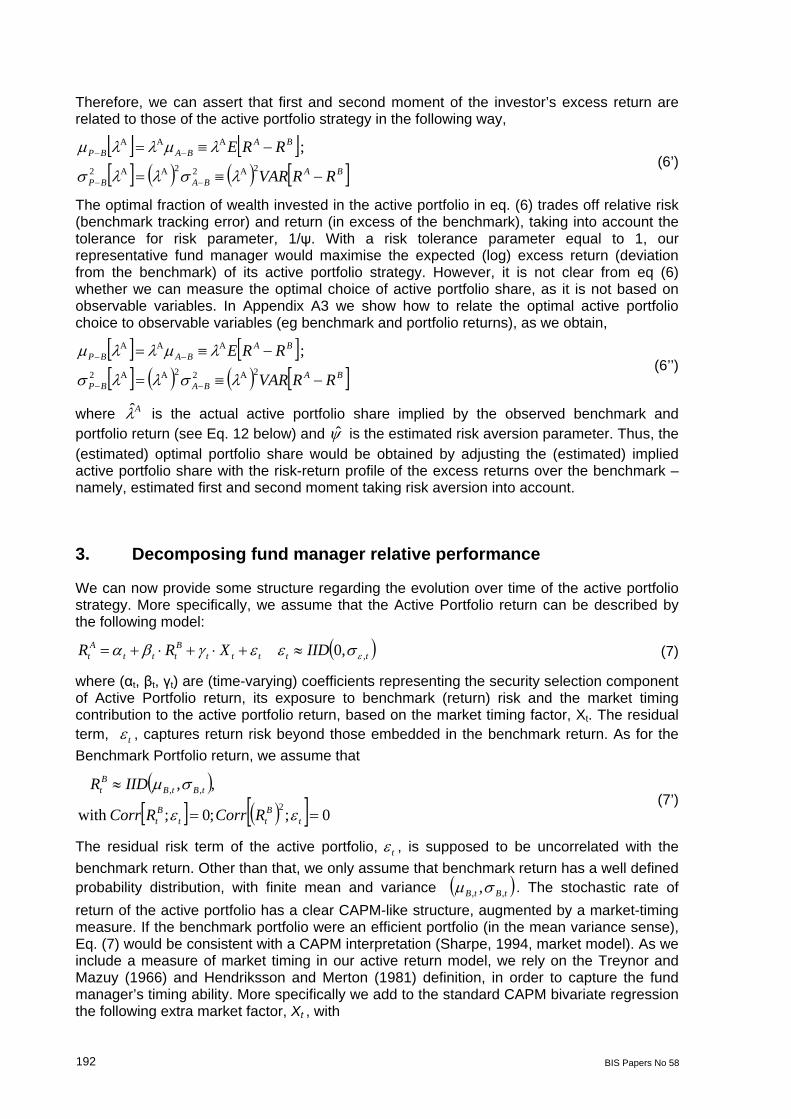
Therefore, we can assert that first and second moment of the investor’s excess return are related to those of the active portfolio strategy in the following way,

BA

BABP

BABABP

RRVAR

RRE

2A22AA2

AAA ;

(6’)

The optimal fraction of wealth invested in the active portfolio in eq. (6) trades off relative risk (benchmark tracking error) and return (in excess of the benchmark), taking into account the tolerance for risk parameter, 1/ψ. With a risk tolerance parameter equal to 1, our representative fund manager would maximise the expected (log) excess return (deviation from the benchmark) of its active portfolio strategy. However, it is not clear from eq (6) whether we can measure the optimal choice of active portfolio share, as it is not based on observable variables. In Appendix A3 we show how to relate the optimal active portfolio choice to observable variables (eg benchmark and portfolio returns), as we obtain,

BA

BABP

BABABP

RRVAR

RRE

2A22AA2

AAA ;

(6’’)

where A is the actual active portfolio share implied by the observed benchmark and portfolio return (see Eq. 12 below) and is the estimated risk aversion parameter. Thus, the (estimated) optimal portfolio share would be obtained by adjusting the (estimated) implied active portfolio share with the risk-return profile of the excess returns over the benchmark – namely, estimated first and second moment taking risk aversion into account.

3. Decomposing fund manager relative performance

We can now provide some structure regarding the evolution over time of the active portfolio strategy. More specifically, we assume that the Active Portfolio return can be described by the following model:

tttttBttt

At IIDXRR ,,0 (7)

where (αt, βt, γt) are (time-varying) coefficients representing the security selection component of Active Portfolio return, its exposure to benchmark (return) risk and the market timing contribution to the active portfolio return, based on the market timing factor, Xt. The residual term, t , captures return risk beyond those embedded in the benchmark return. As for the

Benchmark Portfolio return, we assume that

0;;0;with

,, 2

,,

tBtt

Bt

tBtBBt

RCorrRCorr

IIDR

(7’)

The residual risk term of the active portfolio, t , is supposed to be uncorrelated with the

benchmark return. Other than that, we only assume that benchmark return has a well defined probability distribution, with finite mean and variance tBtB ,, , . The stochastic rate of

return of the active portfolio has a clear CAPM-like structure, augmented by a market-timing measure. If the benchmark portfolio were an efficient portfolio (in the mean variance sense), Eq. (7) would be consistent with a CAPM interpretation (Sharpe, 1994, market model). As we include a measure of market timing in our active return model, we rely on the Treynor and Mazuy (1966) and Hendriksson and Merton (1981) definition, in order to capture the fund manager’s timing ability. More specifically we add to the standard CAPM bivariate regression the following extra market factor, Xt , with


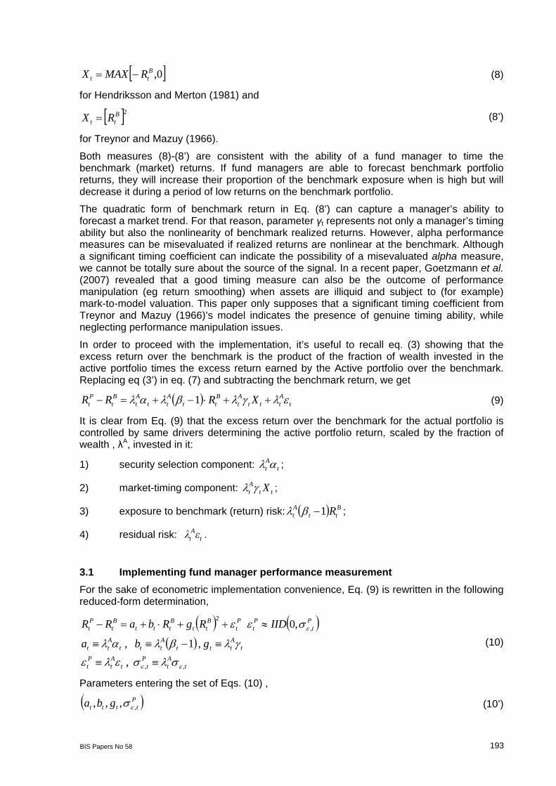
0,Btt RMAXX (8)

for Hendriksson and Merton (1981) and

2Btt RX (8’)

for Treynor and Mazuy (1966).

Both measures (8)-(8’) are consistent with the ability of a fund manager to time the benchmark (market) returns. If fund managers are able to forecast benchmark portfolio returns, they will increase their proportion of the benchmark exposure when is high but will decrease it during a period of low returns on the benchmark portfolio.

The quadratic form of benchmark return in Eq. (8’) can capture a manager’s ability to forecast a market trend. For that reason, parameter γt represents not only a manager’s timing ability but also the nonlinearity of benchmark realized returns. However, alpha performance measures can be misevaluated if realized returns are nonlinear at the benchmark. Although a significant timing coefficient can indicate the possibility of a misevaluated alpha measure, we cannot be totally sure about the source of the signal. In a recent paper, Goetzmann et al. (2007) revealed that a good timing measure can also be the outcome of performance manipulation (eg return smoothing) when assets are illiquid and subject to (for example) mark-to-model valuation. This paper only supposes that a significant timing coefficient from Treynor and Mazuy (1966)’s model indicates the presence of genuine timing ability, while neglecting performance manipulation issues.

In order to proceed with the implementation, it’s useful to recall eq. (3) showing that the excess return over the benchmark is the product of the fraction of wealth invested in the active portfolio times the excess return earned by the Active portfolio over the benchmark. Replacing eq (3’) in eq. (7) and subtracting the benchmark return, we get

1 tAttt

At

Btt

Att

At

Bt

Pt XRRR (9)

It is clear from Eq. (9) that the excess return over the benchmark for the actual portfolio is controlled by same drivers determining the active portfolio return, scaled by the fraction of wealth , λA, invested in it:

1) security selection component: tAt ;

2) market-timing component: ttAt X ;

3) exposure to benchmark (return) risk: Btt

At R1 ;

4) residual risk: tA

t ελ .

3.1 Implementing fund manager performance measurement

For the sake of econometric implementation convenience, Eq. (9) is rewritten in the following reduced-form determination,

tAt

Ptt

At

Pt

tAttt

Attt

Att

Pt

Pt

Pt

Btt

Bttt

Bt

Pt

gba

IIDRgRbaRR

,,

,2

,

, 1 ,

,0

(10)

Parameters entering the set of Eqs. (10) ,

Ptttt gba ,,,, (10’)


are easily amenable to standard econometric estimation technique, as we observe both benchmark and fund manager’s portfolio returns. However we would still be in need of an identification procedure to measure the fraction of wealth, λA, invested in the active portfolio, in order to recover the (hidden active performance) parameters of interest,

ttttAt ,,,,, (10’’)

Chen et al. (2009) derive an interesting generalisation of model (10) that incorporates the non-linear benchmark, replacing the market portfolio in the classical market-timing regression of Treynor and Mazuy (1966). Fund managers are assumed to time the market risk factors by anticipating their impact on the benchmark returns. Such impact may take a non-linear shape.3

Our identification strategy focuses on the level of risk determination for the active portfolio (eg its variance). The adopted key assumption relates the variance of the active portfolio to the variance of the benchmark portfolio by a coefficient, t , assumed to be known in

advance to the fund manager,

2,

22, tBttA (11)

For the sake of simplicity, we set the value of t equal 1 in equation (11), as if the fund

manager would be choosing its active portfolio under the constraint of matching the risk of the benchmark portfolio. As a result, the variance of the active portfolio coincides with the variance of the benchmark return,

2,

2, tBtA (11’)

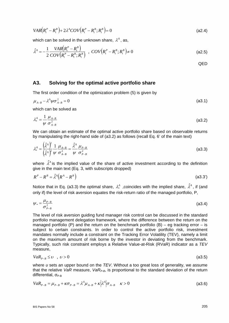
We believe that there would not be much gain in relaxing risk constraint (11’) by choosing different levels of (predetermined) deviation – albeit small – from the benchmark risk. In appendix A2 we prove that under the constraint (11’), the implied share of active portfolio share based on observable returns is given by

B

tBt

Pt

Bt

PtA

RRRCOV

RRVAR

;21ˆ

(12)

Having estimated the unknown parameters (10’) and (12), we can compute parameters (10’’),

2

2,2

, , 1 , ;At

At

tAt

ttA

t

ttA

t

tt

bag

(12’)

For the sake of simplicity, and in common with the classical market-timing models,4 we maintain the hypothesis that returns can be represented by a static ordinary least squares (OLS) model with constant parameters,

3 One of the non linear forms considered in Chen et al. (2009) paper is a quadratic function, which has an

interesting interpretation in terms of systematic coskewness. Asset-pricing models featuring systematic coskewness are developed, for example, by Kraus and Litzenberger (1976). Equation (10) would in fact be equivalent to the quadratic “characteristic line” used by Kraus and Litzenberger. Under their interpretation the coefficient on the squared factor changes does not measure market timing, but measures the systematic coskewness risk. Thus, a fund's return can bear a convex relation to a factor because it holds assets with coskewness risk.

4 Cf Jensen (1968), Treynor and Mazuy (1966) and Henriksson and Merton (1981).


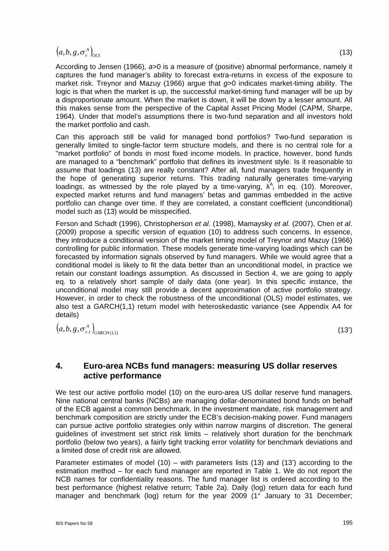
OLSAgba ,,, (13)

According to Jensen (1966), a>0 is a measure of (positive) abnormal performance, namely it captures the fund manager’s ability to forecast extra-returns in excess of the exposure to market risk. Treynor and Mazuy (1966) argue that g>0 indicates market-timing ability. The logic is that when the market is up, the successful market-timing fund manager will be up by a disproportionate amount. When the market is down, it will be down by a lesser amount. All this makes sense from the perspective of the Capital Asset Pricing Model (CAPM, Sharpe, 1964). Under that model’s assumptions there is two-fund separation and all investors hold the market portfolio and cash.

Can this approach still be valid for managed bond portfolios? Two-fund separation is generally limited to single-factor term structure models, and there is no central role for a "market portfolio" of bonds in most fixed income models. In practice, however, bond funds are managed to a “benchmark” portfolio that defines its investment style. Is it reasonable to assume that loadings (13) are really constant? After all, fund managers trade frequently in the hope of generating superior returns. This trading naturally generates time-varying loadings, as witnessed by the role played by a time-varying, λA

t in eq. (10). Moreover, expected market returns and fund managers’ betas and gammas embedded in the active portfolio can change over time. If they are correlated, a constant coefficient (unconditional) model such as (13) would be misspecified.

Ferson and Schadt (1996), Christopherson et al. (1998), Mamaysky et al. (2007), Chen et al. (2009) propose a specific version of equation (10) to address such concerns. In essence, they introduce a conditional version of the market timing model of Treynor and Mazuy (1966) controlling for public information. These models generate time-varying loadings which can be forecasted by information signals observed by fund managers. While we would agree that a conditional model is likely to fit the data better than an unconditional model, in practice we retain our constant loadings assumption. As discussed in Section 4, we are going to apply eq. to a relatively short sample of daily data (one year). In this specific instance, the unconditional model may still provide a decent approximation of active portfolio strategy. However, in order to check the robustness of the unconditional (OLS) model estimates, we also test a GARCH(1,1) return model with heteroskedastic variance (see Appendix A4 for details)

)1,1(,,,,

GARCH

Atgba (13’)

4. Euro-area NCBs fund managers: measuring US dollar reserves active performance

We test our active portfolio model (10) on the euro-area US dollar reserve fund managers. Nine national central banks (NCBs) are managing dollar-denominated bond funds on behalf of the ECB against a common benchmark. In the investment mandate, risk management and benchmark composition are strictly under the ECB’s decision-making power. Fund managers can pursue active portfolio strategies only within narrow margins of discretion. The general guidelines of investment set strict risk limits – relatively short duration for the benchmark portfolio (below two years), a fairly tight tracking error volatility for benchmark deviations and a limited dose of credit risk are allowed.

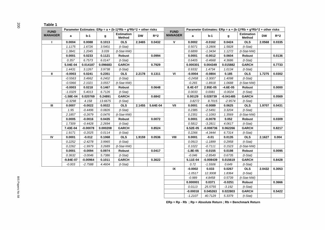
Parameter estimates of model (10) – with parameters lists (13) and (13’) according to the estimation method – for each fund manager are reported in Table 1. We do not report the NCB names for confidentiality reasons. The fund manager list is ordered according to the best performance (highest relative return; Table 2a). Daily (log) return data for each fund manager and benchmark (log) return for the year 2009 (1° January to 31 December;


365 observations) are used.5 The same sample is again considered for the computation of statistical indicators and performance measurement.

Reported parameter values reflect three different estimation methods:

1) Standard OLS (homoskedastic residuals assumption);

2) Robust OLS, (non-gaussian returns; homoskedastic residuals assumption);

3) Maximum-Likelihood (ML), GARCH(1,1) model (heteroskedastic residuals assumption);

Method 1) and 2) assume constant residual variance, 2 . Method 3) include a GARCH(1,1)

variance equation model to correct for residuals heteroskedasticity (see Appendix A4 for details). Parameters testing report t-Student statistics, standard as well as with Newey-West adjustment procedure. Coefficient of Determination, R2, and autocorrelation of residuals test (Durbin-Watson; DW) are also reported.

The best fund managers – ranked according to table 2a by benchmark return out-performance – do show statistically significant parameters. In particular, the market timing performance parameter, g, is positive and significant for seven (out of nine) fund managers. The market portfolio parameter, b, is positive and significant for three fund managers; two of them are also the top performers in the ranking (the third one is found at the bottom). Moreover, there are three other fund managers that display statistically significant, b, with negative sign, however. In this case a negative exposure to market portfolio subtracts from fund performance, since the return of the benchmark turns out to be positive in the sample.

Selectivity appears to be very modest. The Jensen-α parameter, a, is statically significant (at 5% level) for one fund manager only (the third best performer in the ranking). The level of estimated residual autocorrelation (DW statistics) is confined to a range [1.73-2.35] consistent with absence (or modest level) of autocorrelation. The coefficient of determination, R2, based on OLS estimates, is generally low, below 10% for eight out of nine fund managers. More often than not, this is strongly related to the heteroskedasticity of residuals: in seven out of nine cases R2 coefficient jumps to well above 0.5 if the GARCH(1,1) estimates are considered. Changes in residuals volatility should capture risk factors dynamics beyond market portfolio risk (benchmark return) and market-timing risk (non linear or volatility risk implied by the benchmark portfolio). Such changes may reflect predictable, but unobserved (by the econometrician) adjustments in the active portfolio allocation selected by the fund manager (cf Eq. 12’, normalised residuals). These portfolio adjustments may be driven by the dynamics of the risk-return trade-off (eg price-of-risk) faced by active fund managers. The implications of such important risk dynamics are not pursued further here, as they would require a more sophisticated identification strategy – this can be an interesting topic to investigate in future research. These considerations, as long as they are confined to residual risk, do not matter for performance decomposition, as we will see in a moment.

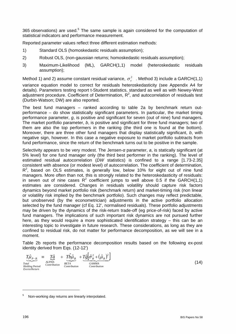
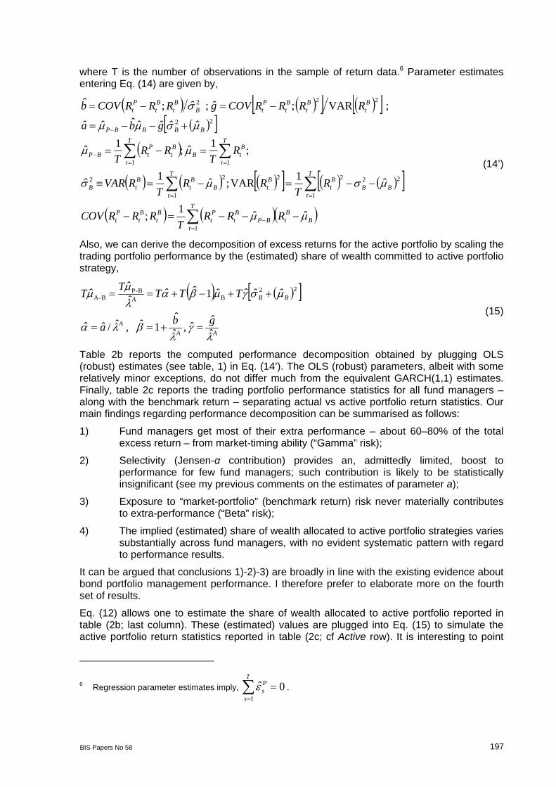
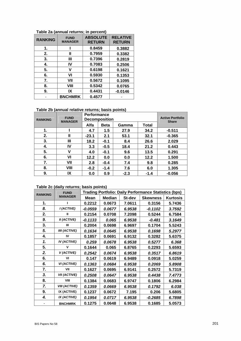
Table 2b reports the performance decomposition results based on the following ex-post identity derived from Eqs. (12-12’)

onContributiGAMMA

BB

onContributiBETA

B

onContributiALPHA

turnExcessHoldingTotal

BP gTbTaTT 22

RePeriod

ˆˆˆˆˆˆˆ

(14)

5 Non-working day returns are linearly interpolated.


where T is the number of observations in the sample of return data.6 Parameter estimates entering Eq. (14) are given by,

T

tB

BtBP

Bt

Pt

Bt

Bt

Pt

T

tBB

Bt

Bt

T

tB

Bt

BtB

T

t

BtB

T

t

Bt

PtBP

BBBBP

Bt

Bt

Bt

PtB

Bt

Bt

Pt

RRRT

RRRCOV

RT

RRT

RVAR

RT

RRT

gba

RRRRCOVgRRRCOVb

1

1

2222

1

22

11

22

222

ˆˆ1;

ˆ1VAR;ˆ1ˆ

;1ˆ ;1ˆ

ˆˆˆˆˆˆˆ

; VAR;ˆ ; ˆ;ˆ

(14’)

Also, we can derive the decomposition of excess returns for the active portfolio by scaling the trading portfolio performance by the (estimated) share of wealth committed to active portfolio strategy,

ˆˆˆ ,ˆ

ˆ1ˆ , ˆ/ˆˆ

ˆˆˆˆ1ˆˆˆˆˆ 22

BB-P

B-A

AA

A

BBA

gba

TTTT

T

(15)

Table 2b reports the computed performance decomposition obtained by plugging OLS (robust) estimates (see table, 1) in Eq. (14’). The OLS (robust) parameters, albeit with some relatively minor exceptions, do not differ much from the equivalent GARCH(1,1) estimates. Finally, table 2c reports the trading portfolio performance statistics for all fund managers – along with the benchmark return – separating actual vs active portfolio return statistics. Our main findings regarding performance decomposition can be summarised as follows:

1) Fund managers get most of their extra performance – about 60–80% of the total excess return – from market-timing ability (“Gamma” risk);

2) Selectivity (Jensen-α contribution) provides an, admittedly limited, boost to performance for few fund managers; such contribution is likely to be statistically insignificant (see my previous comments on the estimates of parameter a);

3) Exposure to “market-portfolio” (benchmark return) risk never materially contributes to extra-performance (“Beta” risk);

4) The implied (estimated) share of wealth allocated to active portfolio strategies varies substantially across fund managers, with no evident systematic pattern with regard to performance results.

It can be argued that conclusions 1)-2)-3) are broadly in line with the existing evidence about bond portfolio management performance. I therefore prefer to elaborate more on the fourth set of results.

Eq. (12) allows one to estimate the share of wealth allocated to active portfolio reported in table (2b; last column). These (estimated) values are plugged into Eq. (15) to simulate the active portfolio return statistics reported in table (2c; cf Active row). It is interesting to point

6 Regression parameter estimates imply, 0ˆ1

T

s

Ps .


out that the two highest ranking fund performances take a short position in the active portfolio. In essence, these fund managers are investing all their money in the benchmark portfolio while selling their active portfolio (-0.51 and -0.36 dollar per dollar of invested wealth) to “buy with the proceeds” additional exposure to the benchmark portfolio. To be sure, their active portfolio strategy is expected to underperform the benchmark! Thus, fund managers can also profit from “inefficient” active strategies – with expected return lower than the benchmark (for given, identical “benchmark” and “active” portfolio risk) – if they are prepared to short them. On the other hand, there are fund managers – with supposedly more promising active portfolio strategies (ranking third, sixth and eight) – that are doing exactly the opposite: they are shorting the benchmark to finance with the proceeds additional exposure to their active strategy. In this case, their allocated share to their active strategy has to be larger than one (2.03, 1.50 and 1.31, respectively). Only three fund managers (out of nine) avoid leveraging their portfolio one way or the other; all of them end up in the middle of the performance ranking.

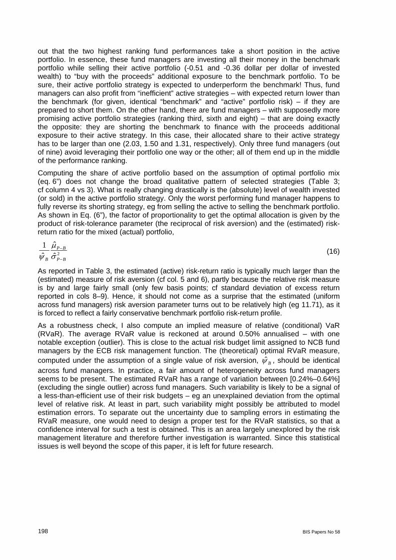
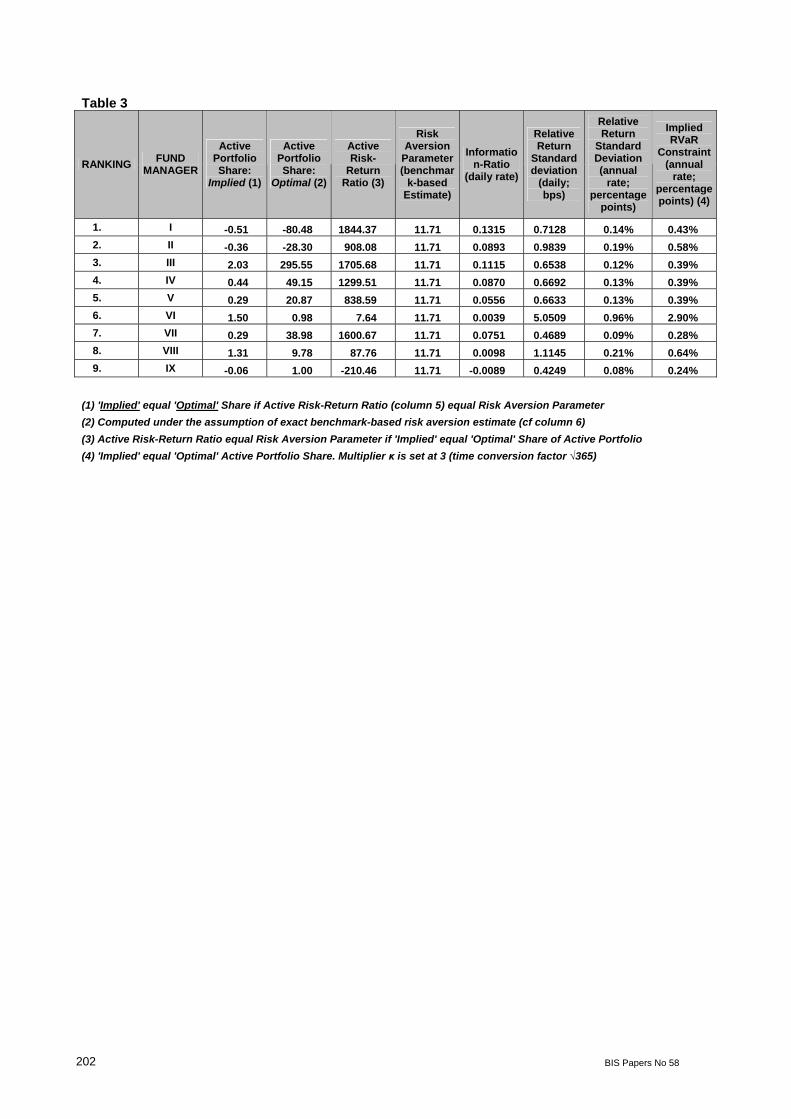
Computing the share of active portfolio based on the assumption of optimal portfolio mix (eq. 6”) does not change the broad qualitative pattern of selected strategies (Table 3; cf column 4 vs 3). What is really changing drastically is the (absolute) level of wealth invested (or sold) in the active portfolio strategy. Only the worst performing fund manager happens to fully reverse its shorting strategy, eg from selling the active to selling the benchmark portfolio. As shown in Eq. (6”), the factor of proportionality to get the optimal allocation is given by the product of risk-tolerance parameter (the reciprocal of risk aversion) and the (estimated) risk-return ratio for the mixed (actual) portfolio,

2ˆˆ

ˆ1

BP

BP

B

(16)

As reported in Table 3, the estimated (active) risk-return ratio is typically much larger than the (estimated) measure of risk aversion (cf col. 5 and 6), partly because the relative risk measure is by and large fairly small (only few basis points; cf standard deviation of excess return reported in cols 8–9). Hence, it should not come as a surprise that the estimated (uniform across fund managers) risk aversion parameter turns out to be relatively high (eg 11.71), as it is forced to reflect a fairly conservative benchmark portfolio risk-return profile.

As a robustness check, I also compute an implied measure of relative (conditional) VaR (RVaR). The average RVaR value is reckoned at around 0.50% annualised – with one notable exception (outlier). This is close to the actual risk budget limit assigned to NCB fund managers by the ECB risk management function. The (theoretical) optimal RVaR measure, computed under the assumption of a single value of risk aversion, B , should be identical across fund managers. In practice, a fair amount of heterogeneity across fund managers seems to be present. The estimated RVaR has a range of variation between [0.24%–0.64%] (excluding the single outlier) across fund managers. Such variability is likely to be a signal of a less-than-efficient use of their risk budgets – eg an unexplained deviation from the optimal level of relative risk. At least in part, such variability might possibly be attributed to model estimation errors. To separate out the uncertainty due to sampling errors in estimating the RVaR measure, one would need to design a proper test for the RVaR statistics, so that a confidence interval for such a test is obtained. This is an area largely unexplored by the risk management literature and therefore further investigation is warranted. Since this statistical issues is well beyond the scope of this paper, it is left for future research.


5. Concluding remarks

The question of whether fund managers adopt an optimal active-passive risk allocation is addressed using in a straightforward extension of the T-B model. The essential insight into the T-B analysis is that the optimal combination of the active portfolio and a passive benchmark portfolio is itself a straightforward portfolio optimization problem. The T-B model allows fund managers to select the mix of active and passive portfolio that maximizes the (active) Sharpe-ratio performance indicator. The investment allocation assigned to the active portfolio strategy increases with the level of alpha (excess return over the benchmark portfolio) and decreases with the degree of unsystematic risk of the invested portfolio. The T-B model is here adapted and made operational as a tool for performance measurement. More specifically, the sources of fund management performance are isolated (selectivity vs market timing); the combination of active and passive risk exposures are estimated; individual fund manager portfolio choice (eg the active vs passive mix) and the related risk budget absorption are tested against the hypothesis of optimal design for the alpha-generating portfolio strategy.

The T-B model is applied to a sample of US dollar reserve management portfolios (owned by the ECB) invested in high grade dollar denominated bonds. Model parameters are estimated using standard OLS and GARCH(1,1) technique on daily portfolio returns for each fund managers. A performance decomposition, based on the well known selectivity and market-timing factors, is computed for each fund manager. The best fund managers show statistically significant outperformance against the benchmark. By far, market timing is its main driver. Selectivity appears to be very modest. These results are not very surprising after all, in that low credit risk and highly liquid securities dominate portfolio selection. Thus, very few opportunities are probably available to fund managers looking for (systematically) profitable bond-picking activity.

As far as the risk-return profile of the active portfolio is concerned, it appears that some of the best fund managers outperformance is realised by shorting the active portfolio with respect to the benchmark composition. Such portfolios are (rightly) shorted, because their equivalent long position would imply a negative (expected) excess return. Thus, long portfolios that are inefficient with respect to the their benchmark (negative excess return) can be turned into positive-alpha yielding portfolios provided that they are shorted. The long vs short choice of active portfolio requires a certain degree of fund manager ability in predicting the sign of excess returns. This ability can be seen as an additional source of fund manager’s outperformance, beyond the skill in anticipating the returns of the benchmark portfolio (market timing contribution).

Based on the model parameters estimates, I derive a measure of risk aversion (uniform across fund managers), consistent with the optimal active portfolio choice hypothesis. Such measure of risk turns out to be relatively high, as it is forced to reflect a fairly conservative benchmark portfolio risk-return profile. I also compute an implied measure of relative risk exposure, based on the concept of conditional Relative VaR (RVaR). The implied average level of RVaR (0.50% annualised) is close to the actual risk budget limit assigned to fund managers. However, a fair amount of heterogeneity across fund managers is found to be present, as the range of variation of (optimal implied) RVaR measures is material. Such variability across fund managers is a likely signal of inefficient use of their risk budget – eg a deviation from the optimal level of relative risk. At least in part, such variability could also be attributed to model estimation errors. To separate out the uncertainty due to sampling errors in estimating the RVaRs, one would need to design a proper test for the RVaR statistics, so that a confidence interval for such a test is obtained. This is an area largely unexplored by the risk management literature and therefore requires further investigation. For this reason it is left for future research.

200

BIS

Papers N

o 58

Table 1

Parameter Estimates: ERp = a + (b-1)*Rb + g*Rb^2 + other risks Parameter Estimates: ERp = a + (b-1)*Rb + g*Rb^2 + other risks FUND

MANAGER a b-1 g Estimation

Method DW R^2

FUND MANAGER a b-1 g

Estimation Method

DW R^2

I 0.0004 0.0088 0.1013 OLS 2.3465 0.0432 V 0.0002 -0.0162 0.0424 OLS 2.0568 0.0335

1.1175 1.6726 3.5401 (t-Stat) 0.5071 -3.2806 1.5828 (t-Stat)

1.3841 1.2045 3.039 (t-Stat-NW) 0.6899 -1.3434 1.1272 (t-Stat-NW)

0.0001 0.0233 0.1121 Robust 0.0994 0.0001 -0.0012 0.0604 Robust 0.0136

0.357 6.7573 6.0147 (t-Stat) 0.6405 -0.4668 4.3686 (t-Stat)

5.04E-04 0.014187 0.096683 GARCH 0.7929 0.000301 0.004349 0.015882 GARCH 0.7733

1.4431 3.1267 3.9738 (t-Stat) 0.9332 1.4734 1.0134 (t-Stat)

II -0.0003 0.0241 0.2351 OLS 2.2178 0.1311 VI -0.0004 -0.0804 0.185 OLS 1.7275 0.0302

-0.5563 3.4662 6.2402 (t-Stat) -0.2458 -3.3007 1.4098 (t-Stat)

-0.5966 2.1021 3.0557 (t-Stat-NW) -0.265 -1.8918 1.0688 (t-Stat-NW)

-0.0003 0.0218 0.1467 Robust 0.0648 8.4E-07 2.95E-05 -4.6E-05 Robust 0.0000

-1.0329 5.4013 6.7126 (t-Stat) 0.0033 0.0081 -0.0024 (t-Stat)

-1.58E-04 0.020769 0.24891 GARCH 0.6842 0.00129 0.028739 -0.041485 GARCH 0.0569

-0.3298 4.158 13.6675 (t-Stat) 3.8272 8.7015 -2.9574 (t-Stat)

III 0.0007 -0.0022 0.0022 OLS 2.1455 5.64E-04 VII 0.0001 -0.0089 0.0625 OLS 1.9707 0.0431

1.95 -0.4496 0.0826 (t-Stat) 0.2385 -2.5491 3.3204 (t-Stat)

2.1857 -0.2679 0.0476 (t-Stat-NW) 0.2351 -1.1093 1.3569 (t-Stat-NW)

0.0005 -0.0016 0.0435 Robust 0.0072 0.0001 -0.0078 0.052 Robust 0.0309

1.7309 -0.4428 2.2694 (t-Stat) 0.5812 -3.2811 4.0617 (t-Stat)

7.43E-04 -0.00078 0.000208 GARCH 0.8524 6.52E-05 -0.008736 0.062266 GARCH 0.8217

1.9171 -0.2025 0.0114 (t-Stat) 0.2266 -4.3444 6.7314 (t-Stat)

IV 0.0001 -0.012 0.1068 OLS 1.9159 0.0536 VIII 0.0001 -0.01 0.0135 OLS 2.1627 0.004

0.2252 -2.4278 3.9965 (t-Stat) 0.0913 -1.1899 0.2958 (t-Stat)

0.2262 -1.9979 3.2689 (t-Stat-NW) 0.1022 -0.7111 0.1523 (t-Stat-NW)

0.0001 -0.0094 0.0974 Robust 0.0417 -1.8E-05 -0.0155 0.0198 Robust 0.0095

0.3632 -3.0046 5.7386 (t-Stat) -0.046 -2.8549 0.6735 (t-Stat)

-9.84E-07 -0.00964 0.1011 GARCH 0.3622 5.11E-04 -0.008439 0.015619 GARCH 0.8428

-0.003 -2.7588 4.4604 (t-Stat) 0.72 -1.5506 0.649 (t-Stat)

IX -0.0002 0.033 0.0267 OLS 2.0432 0.3053

-1.0517 12.3008 1.8364 (t-Stat)

-0.989 4.8458 0.5739 (t-Stat-NW)

0.000001 0.0371 -0.0251 Robust 0.3666

0.0113 25.5755 -3.192 (t-Stat)

-0.00018 0.045263 0.022803 GARCH 0.5422

-1.2107 40.7129 5.3379 (t-Stat)

ERp = Rp - Rb ; Rp = Absolute Return ; Rb = Benchmark Return


Table 2a (annual returns; in percent)

RANKING FUND MANAGER

ABSOLUTE RETURN

RELATIVE RETURN

1. I 0.8459 0.3882 2. II 0.7959 0.3382 3. III 0.7396 0.2819 4. IV 0.7083 0.2506 5. V 0.6198 0.1621 6. VI 0.5930 0.1353 7. VII 0.5672 0.1095 8. VIII 0.5342 0.0765 9. IX 0.4431 -0.0146 - BNCHMRK 0.4577 -

Table 2b (annual relative returns; basis points) Performance Decomposition RANKING

FUND MANAGER

Alfa Beta Gamma Total

Active Portfolio Share

1. I 4.7 1.5 27.9 34.2 -0.511 2. II -23.1 2.1 53.1 32.1 -0.365 3. III 18.2 -0.1 8.4 26.6 2.029 4. IV 3.3 -0.5 18.4 21.2 0.443 5. V 4.0 -0.1 9.6 13.5 0.291 6. VI 12.2 0.0 0.0 12.2 1.500 7. VII 2.8 -0.4 7.4 9.8 0.285 8. VIII -0.2 -1.4 7.6 6.0 1.305 9. IX 0.0 0.9 -2.3 -1.4 -0.056

Table 2c (daily returns; basis points) Trading Portfolio: Daily Performance Statistics (bps)

RANKING FUND

MANAGER Mean Median St-dev Skewness Kurtosis 1. I 0.2212 0.0673 7.0611 0.3156 5.7436 8. I (ACTIVE) -0.0559 0.0677 6.9538 -0.1102 3.7592 2. II 0.2154 0.0708 7.2098 0.5244 6.7584 9. II (ACTIVE) -0.1133 0.065 6.9538 -0.481 3.1649 3. III 0.2004 0.0698 6.9697 0.1704 5.5243 5. IIII (ACTIVE) 0.1634 0.0645 6.9538 0.1698 5.2977 4. IV 0.1857 0.0691 6.9132 0.3282 5.6375 1. IV (ACTIVE) 0.259 0.0678 6.9538 0.5277 6.368 5. V 0.1644 0.065 6.8765 0.2293 5.6593 2. V (ACTIVE) 0.2542 0.0674 6.9538 0.3517 6.8619 6. VI 0.147 0.0619 6.9489 0.0918 5.0259 6. VI (ACTIVE) 0.1363 0.0684 6.9538 0.2069 5.8908 7. VII 0.1627 0.0695 6.9141 0.2572 5.7319 3. VII (ACTIVE) 0.2508 0.0647 6.9538 0.4438 7.4773

8. VIII 0.1384 0.0683 6.9747 0.1806 6.2984

7. VIII (ACTIVE) 0.1359 0.0669 6.9538 0.1792 6.038 9. IX (ACTIVE) 0.1237 0.0672 7.195 0.206 5.6805 4. IX (ACTIVE) 0.1954 0.0717 6.9538 -0.2685 6.7898

- BNCHMRK 0.1275 0.0648 6.9538 0.1685 5.0573


Table 3

RANKING FUND

MANAGER

Active Portfolio Share:

Implied (1)

Active Portfolio Share:

Optimal (2)

Active Risk-

Return Ratio (3)

Risk Aversion

Parameter (benchmar

k-based Estimate)

Information-Ratio

(daily rate)

Relative Return

Standard deviation

(daily; bps)

Relative Return

Standard Deviation (annual

rate; percentage

points)

Implied RVaR

Constraint (annual

rate; percentage points) (4)

1. I -0.51 -80.48 1844.37 11.71 0.1315 0.7128 0.14% 0.43%

2. II -0.36 -28.30 908.08 11.71 0.0893 0.9839 0.19% 0.58%

3. III 2.03 295.55 1705.68 11.71 0.1115 0.6538 0.12% 0.39%

4. IV 0.44 49.15 1299.51 11.71 0.0870 0.6692 0.13% 0.39%

5. V 0.29 20.87 838.59 11.71 0.0556 0.6633 0.13% 0.39%

6. VI 1.50 0.98 7.64 11.71 0.0039 5.0509 0.96% 2.90%

7. VII 0.29 38.98 1600.67 11.71 0.0751 0.4689 0.09% 0.28%

8. VIII 1.31 9.78 87.76 11.71 0.0098 1.1145 0.21% 0.64%

9. IX -0.06 1.00 -210.46 11.71 -0.0089 0.4249 0.08% 0.24%

(1) 'Implied' equal 'Optimal' Share if Active Risk-Return Ratio (column 5) equal Risk Aversion Parameter

(2) Computed under the assumption of exact benchmark-based risk aversion estimate (cf column 6)

(3) Active Risk-Return Ratio equal Risk Aversion Parameter if 'Implied' equal 'Optimal' Share of Active Portfolio

(4) 'Implied' equal 'Optimal' Active Portfolio Share. Multiplier κ is set at 3 (time conversion factor √365)


Appendix

A1. Relative asset allocation: active vs benchmark portfolio

Let us consider a typical investment mandate. A fund manager is assigned the task to beat a benchmark portfolio over a specified time horizon. The benchmark portfolio, as specified in the mandate, should be attainable and investable. Depending on his expertise, the portfolio manager can overweight certain asset classes and/or securities and by the same token underweight others, thus building a zero-investment active portfolio. The composition of this active portfolio reflects the selection bets made by the portfolio manager.

Let us assume that there are {i=1,N } asset classes/securities to invest our portfolio. Its shares at time t can be represented as a vector of portfolio holdings adding up to 1:

N

i

Pit

PNt

Pt

Pt

Pt

1,,2,1, 1 with ,,...,, (a1.1)

Our fund manager confronts a known Benchmark Portfolio, B, with a given structure,

N

i

Bit

BNt

Bt

Bt

Bt

1,,2,1, 1 with ,,...,, (a1.2)

In constructing her Managed Portfolio, P (eq, a1.1), our fund manager separates her active investment strategies in two related steps. In her first step she tries to construct an Active Portfolio, A, which in her view differs from the benchmark in various desirable ways

N

i

Ait

ANt

At

At

At

1,,2,1, 1 with ,,...,, (a1.3)

In her second step, she has to decide how much wealth she would commit to her Active Portfolio, A, in building her managed portfolio P. More specifically she has to set aside a

fraction, At , of her total wealth (equal to 1) to be invested in portfolio A and the remaining

fraction, At1 , in the benchmark holdings. Thus, her Managed Portfolio has the following

structure:

componentBenchmark

Bt

At

componentActive

At

At

PortfolioManaged

Pt 1

(a1.4)

Thus, her managed portfolio, P, turns out to be a combination of both active and passive

portfolios, with exposure to the active component regulated by the amount, At ,

We can rewrite Eq. (a1.4) highlighting the Managed Portfolio deviations from the benchmark holdings,

holdingsPortfolio BenchmarkActive and betweenDifference

Bt

At

SharePortfolioActive

At

arkthe BenchmfromDeviation PortfolioManaged

Bt

Pt

(a1.5)

The left-hand-side holdings in Eq. (a1.5) can be observed directly by inspecting our fund manager’s allocation, whereas the right-hand side decomposition is not known, unless we were to know in detail the two steps procedure highlighted above, namely the Active Portfolio

holdings, At , as well the associated fraction of wealth, A

t , selection process. However, we

can argue that if we happen to know the fraction of wealth invested in the Active Portfolio, we


can easily recover the implied holdings of the Active Portfolio by inverting Eq. (a1.5) as follows

Bt

PtA

t

Bt

At

1 (a1.6)

Our suggested two steps procedure may sound a bit contrived. Why bother paying attention to the decomposition suggested by the right-hand side of Eq. (a1.5) if what ultimately matters are only the bets (deviations from the benchmarks holdings) laid out in its left-hand side ? As investors, we are interested in the fund manager ability of selecting portfolio that can beat the benchmark. However, we can infer from decomposition (a1.5) that there perhaps be a wider range of active strategies than we have thought enabling us to achieve the extra-performance target. To appreciate such implication, let us transform decomposition (a1.5) in its return equivalent format (recall Eq. 3’ in the main text)

Bt

At

At

Bt

Pt RRRR (a1.7)

Eq. (a1.7) suggests that, in principle, any active strategies (Portfolio A) can be used in order to beat the benchmark, provided that the share of wealth allocated to it (exposure) has the appropriate sign – long or short – depending upon the its expected performance relative to the benchmark. In brief, if the fund manager is convinced that her active Portfolio, A, can

beat the benchmark, she would certainly want to be long portfolio A ( 0At ). Conversely,

she may well come across an active portfolio, A, which (she believes) would very likely underperform the benchmark. Such underperforming (active) portfolio can equally provide a perfectly good foundation for a successful active strategy, if the appropriate short exposure

( 0At ) is chosen. Thus, the set of active strategies (portfolios A) seems much wider than

we tend to believe. It all hinges upon the fund manager ability to assess the risk return profile of her selected Active Portfolio, A, vs the returns of the benchmark In the following paragraphs we illustrate several identification procedure for the share of wealth allocated to

active strategies, At ,based on a the risk of the active portfolio, A.

A2. Identifying the implied share of active portfolio return

To derive the implied share invested in the Active Portfolio one need to multiply both side of

constraint (11) by the square of the fraction of wealth, 2A , invested in the active portfolio,

Bt

AAt

A RVARRVAR2

(a2.1)

The left-hand side of eq. (a2.1) can be rewritten using the definition laid out in Eq. (3’):

Bt

ABt

ABt

Pt RVARRRRVAR

2 (a2.2)

Eq. (a2.2) now depends entirely upon observable variables – benchmark and fund

manager’s returns – and the unknown value, At . It is convenient to develop the variance on

the left-hand in eq. (a2.2),

Bt

ABt

Bt

Pt

ABt

Pt

Bt

ABt

Pt RVARRRRCOVRRVARRRRVAR

2;2 (a2.3)

and equate the right-hand side of eq. (a2.2)- and (a2.3). As the term Bt

At RVAR

2 cancels

out, we are left with the following equation,


0;2 Bt

Bt

Pt

ABt

Pt RRRCOVRRVAR (a2.4)

which can be solved in the unknown share, A , as,

0; ,

;21ˆ

Bt

Bt

PtB

tBt

Pt

Bt

PtA RRRCOV

RRRCOV

RRVAR (a2.5)

QED

A3. Solving for the optimal active portfolio share

The first order condition of the optimization problem (5) is given by

02A BABA (a3.1)

which can be solved as

2*1

BA

BAA

(a3.2)

We can obtain an estimate of the optimal active portfolio share based on observable returns by manipulating the right-hand side of (a3.2) as follows (recall Eq. 6’ of the main text)

222

2

*

ˆ1ˆ

ˆ

BP

BPA

BA

BA

A

AA

(a3.3)

where A is the implied value of the share of active investment according to the definition give in the main text (Eq. 3, with subscripts dropped)

BAABP RRRR (a3.3’)

Notice that in Eq. (a3.3) the optimal share, A* ,coincides with the implied share, A , if (and

only if) the level of risk aversion equates the risk-return ratio of the managed portfolio, P,

2*BP

BP

(a3.4)

The level of risk aversion guiding fund manager risk control can be discussed in the standard portfolio management delegation framework, where the difference between the return on the managed portfolio (P) and the return on the benchmark portfolio (B) – eg tracking error – is subject to certain constraints. In order to control the active portfolio risk, investment mandates normally include a constraint on the Tracking Error Volatility (TEV), namely a limit on the maximum amount of risk borne by the investor in deviating from the benchmark. Typically, such risk constraint employs a Relative Value-at-Risk (RVaR) indicator as a TEV measure,

0 , BPVaR (a3.5)

where υ sets an upper bound on the TEV. Without a too great loss of generality, we assume that the relative VaR measure, VaRP-B, is proportional to the standard deviation of the return differential, σP-B

0 BAA

BAA

BPBPBPVaR (a3.6)


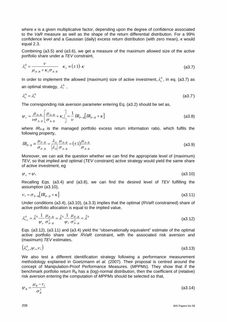
where κ is a given multiplicative factor, depending upon the degree of confidence associated to the VaR measure as well as the shape of the return differential distribution. For a 99% confidence level and a Gaussian (daily) excess return distribution (with zero mean), κ would equal 2.3.

Combining (a3.5) and (a3.6), we get a measure of the maximum allowed size of the active portfolio share under a TEV constraint,

1 BABA

A (a3.7)

In order to implement the allowed (maximum) size of active investment, A , in eq. (a3.7) as

an optimal strategy, A* ,

AA* (a3.7’)

The corresponding risk aversion parameter entering Eq. (a3.2) should be set as,

BPBP

BA

BA

BA

BA IRIR1

(a3.8)

where IRP-B is the managed portfolio excess return information ratio, which fulfils the following property,

BA

BA

BA

BA

A

A

BP

BPBPIR

1 (a3.9)

Moreover, we can ask the question whether we can find the appropriate level of (maximum) TEV, so that implied and optimal (TEV constraint) active strategy would yield the same share of active investment, eg

* (a3.10)

Recalling Eqs. (a3.4) and (a3.8), we can find the desired level of TEV fulfilling the assumption (a3.10),

BPBP IR* (a3.11)

Under conditions (a3.4), (a3.10), (a.3.3) implies that the optimal (RVaR constrained) share of active portfolio allocation is equal to the implied value,

A

BP

BPA

BP

BPAA

ˆ1ˆ1ˆ2

*2,

(a3.12)

Eqs. (a3.12), (a3.11) and (a3.4) yield the “observationally equivalent” estimate of the optimal active portfolio share under RVaR constraint, with the associated risk aversion and (maximum) TEV estimates,

**, ,, A (a3.13)

We also test a different identification strategy following a performance measurement methodology explained in Goetzmann et al. (2007). Their proposal is centred around the concept of Manipulation-Proof Performance Measures. (MPPMs). They show that if the benchmark portfolio return RB has a (log)-normal distribution, then the coefficient of (relative) risk aversion entering the computation of MPPMs should be selected so that,

2B

fBB

r

(a3.14)


where rf measures the risk-free rate of return. Since MPPMs ae typically associated with some benchmark portfolio, in the absence of any private information the MPPM should score the chosen benchmark highly.

Goetzmann et al. (2007) show that this would be the implication of eq. (a3.4) in computing their suggested MPPMs. What does it mean for a measure to be manipulation-free? Intuitively, if a manager has no private information and markets are efficient, then holding some benchmark portfolio, possibly levered, should maximize the measure’s expected value. The benchmark portfolio might coincide with the market-portfolio, but in some contexts other benchmarks could be appropriate. Static manipulation is the tilting of the portfolio away from the (levered) benchmark even when there is no informational reason to do so. Dynamic manipulation is altering the portfolio over time based on past performance rather than on new information. A good performance measure penalises uninformed manipulation of both types in ranking fund managers’ returns. Substituting the benchmark-based risk aversion measure (a3.14) into the optimal active portfolio share (eq. a3.3), we obtain,

2*,

ˆ

BP

BP

B

AA

B

(a3.15)

A4. GARCH model for residual risk in the active portfolio

The error terms in the least-square model (10)-(13) are assumed to be homoskedastic (the same variance at any given data point). Sample data in which the variances of the error terms are not equal – the error terms may reasonably be expected to be larger for some points or ranges of the data than for others – are said to suffer from heteroskedasticity. The standard warning is that in the presence of heteroskedasticity, the regression coefficients for an ordinary least squares regression are still unbiased, but the standard errors and confidence intervals estimated by conventional procedures will be too narrow, giving a false sense of precision. Instead of considering this as a problem to be corrected, ARCH /GARCH models treat heteroskedasticity as a variance to be modelled. As a result, not only are the deficiencies of least squares corrected, but a prediction is computed for the variance of each error term. The ARCH/GARCH models, which stand for autoregressive conditional heteroskedasticity and generalized autoregressive conditional heteroskedasticity, are designed to deal with just this set of issues.

The GARCH(1,1) is probably the simplest and most robust of the family of volatility models. Since we are dealing with a relatively short sample (one year of daily data), higher order models – which would include additional lags – are unlikely to add much value. The GARCH model for variance looks like this (omitting superscript A):

21

21,

2,

2, ttt (a4.1)

where 2,t defines the variance of the residuals of model (10). I estimate the constants

parameters ;;2, . Updating Eq, (4.1) simply requires knowing the previous forecast,

21, t , and (squared) residual term, 2

1, t . The weights are ,,1 and the long run

average variance is given by 12, . This latter is just the unconditional variance.

Thus, the GARCH(1,1) model is mean reverting and conditionally heteroskedastic, but have a constant unconditional variance. It should be noted that this only works if , and only really

makes sense if the weights are positive, requiring 0;;2, .

Parameters in eqs. (10) and (a4.1) are jointly estimated using Maximum Likelihood under the assumption of constant coefficients (eg using parameters’ list, 13’). The GARCH(1,1)


estimates are included in Table1. Reported standard errors are computed using the robust method of Bollerslev-Wooldridge. The coefficients in the variance equation are omitted here to save space and are available upon request from the author. The variance coefficients always sum up to a number less than one which is required in order to have a mean reverting variance process. In certain cases the sum is very close to one, therefore this process only mean reverts slowly. Standard Errors and p-values for parameters’ list (13’) are reported in Table 1.

The standardized residuals are examined for autocorrelation. In most cases, the autocorrelation is dramatically reduced from that observed in the portfolio returns themselves. Applying the same test for autocorrelation, we find the p-values are about 0.5 or more indicating that we can always accept the hypothesis of “no residual ARCH”. As a result, we obtain a larger R2 (coefficient of determination) statistics than standard OLS estimates, as the unanticipated residual variance component is drastically reduced by GARCH(1,1) variance prediction model.

References

Admati, Anat, Sudipto Bhattacharya, Paul Pfleiderer and Stephen A. Ross, (1986) On Timing and Selectivity” Journal of Finance 61, pp. 715–32.

Aragon, George, (2005), “Timing multiple markets: Theory and Evidence from Balanced Mutual Funds”, working paper, Arizona State.

Aragon, George, and Wayne Ferson, (2007), “Portfolio Performance Evaluation, Foundations and Trends in Finance”, Now Publishers vol. 2, No. 2, pp. 83–190.

Blake, Christopher R., Edwin J. Elton and Martin J. Gruber, (1993), “The Performance of Bond Mutual Funds”, Journal of Business 66, pp. 371–403.

Brown, David T. and William J. Marshall, (2001), “Assessing Fixed Income Manager Style and Performance from Historical Returns”, Journal of Fixed Income, 10 (March).

Brown, K. and C. Tiu (2010) “Do Endowment Funds Select the Optima Mix of Active and Passive Risks ? ”, Journal of Investment Management, vol. 8 , n.1, pp. 1–25.

Burmeister, C., H. Mausser and R. Mendoza (2005) “Actively Managing Tracking Error”. Journal of Asset Management, Vol.5, n. 6, pp. 410–22.

Chen Yong, Wayne Ferson Helen Peters, (2009) “Measuring the Timing Ability and Performance of Bond Mutual Funds”, Journal of Financial Economics,

Comer, G., V. Boney and L. Kelley, (2009) “Timing the Investment Grade Securities Market: Evidence from High Quality Bond Funds, Journal of Empirical Finance 16, pp. 55–69.

Elton, Edwin, Martin J. Gruber and Christopher R. Blake, (1995) “Fundamental Economic Variables, Expected returns and Bond Fund Performance” Journal of Finance 50, 1229–56.

Elton, Edwin, Martin J. Gruber and Christopher R. Blake, 2001, A first look at the Accuracy of the CRSP and Morningstar Mutual fund databases, Journal of Finance 56, 2415–30.

Ferson, W., Tyler Henry and Darren Kisgen (2006), Evaluating Government Bond Funds using Stochastic Discount Factors, Review of Financial Studies 19, 423–55.

Ferson, W., S. Sarkissian and T. Simin, (2008) “Asset Pricing Models with Conditional Alphas and Betas: The Effects of Data Snooping and Spurious Regression”, Journal of Financial and Quantitative Analysis 43, pp. 331–54.


Goetzmann, W. N., Ingersoll Jr, J. E., Spiegel, M. I., and Welch, I., 2007, “Portfolio Performance Manipulation and Manipulation–Proof Performance Measures,” Review of Financial Studies, 20, 1503–46.

Grinold, R. and R. Kahn (2000). Active Portfolio Management, 2nd edn. New York: McGraw–Hill.

Henriksson, R. and R. Merton (1981), “On Market Timing and Investment Performance II. Statistical Procedures for Evaluating Forecasting Skills.” Journal of Business 54 (1981), pp. 513–33.

Jorion, P. (2003) “Portfolio Optimization with Tracking-Error Constraints” Financial Analysts Journal, Vol.59, Iss.5 (Sep/Oct), pp. 70–82.

Kane, A., Kim, T., and H. White (2003). “Active Portfolio Management: The Power of the Treynor-Black Model,” Working Paper, University of California, San Diego.

Kraus, Alan and Robert Litzenberger, (1976), “Skewness Preference and the Valuation of Risky Assets”, Journal of Finance 31, pp. 1085–100.

Litterman, R. and J. Scheinkman, (1991) “Common Factors Affecting Bond Returns”, Journal of Fixed Income, 1.

Roll, R. (1992) “A Mean/Variance Analysis of Tracking Error”. The Journal of Portfolio Management, Summer, pp. 13–22.

Sharpe, W.F. (1966) “Mutual Fund Performance” Journal of Business, January, pp. 119–38.

Sharpe, W. F. (1992) “Asset Allocation: Management Style and Performance Peasurement”, Journal of Portfolio Management 18, 7–19.

Sharpe, W.F. (1994) “The Sharpe Ratio” The Journal of Portfolio Management, Fall, pp. 49–58.

Treynor, J. and F. Black (1973) “How to Use Security Analysis to Improve Portfolio Selection,” Journal of Business 46, pp. 66–86.

Treynor, J. and K. Mazuy (1966) “Can Mutual Funds Outguess the Market ? ” Harvard Business Review 44, p.131–6.

Optimal active portfolio management and relative performance drivers ... · Optimal active...

Documents

Transcript of Optimal active portfolio management and relative performance drivers ... · Optimal active...