1

OOppttiiccaall wwaavveegguuiiddee aannaallyyssiiss uussiinngg

BBeeaamm PPrrooppaaggaattiioonn MMeetthhoodd

Term Paper for “Introduction to Optoelectronics” spring 2006

Prof. Frank Barnes

Page 10: My MATLAB® implementation of double slit diffraction

Using Beam Propagation Method

Sri Rama Prasanna Pavani

pavani@colorado.edu

Micro-Optical Imaging Systems Laboratory

University of Colorado at Boulder

2

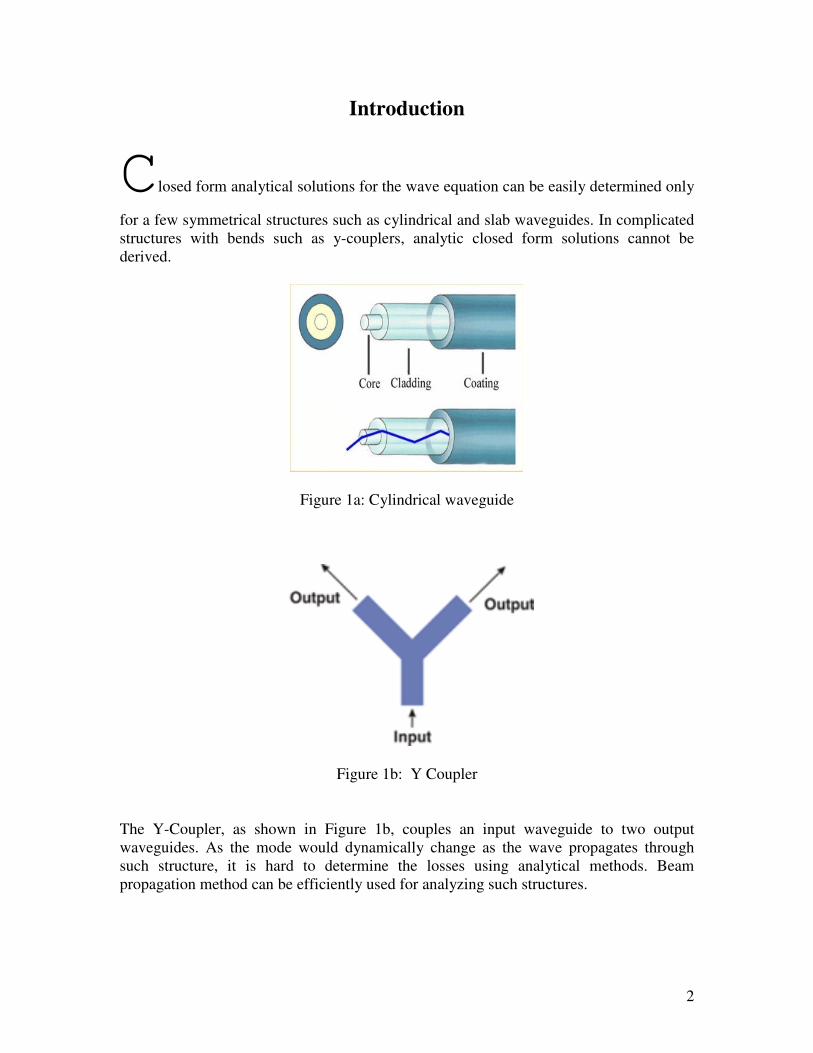
Introduction

Closed form analytical solutions for the wave equation can be easily determined only

for a few symmetrical structures such as cylindrical and slab waveguides. In complicated

structures with bends such as y-couplers, analytic closed form solutions cannot be

derived.

Figure 1a: Cylindrical waveguide

Figure 1b: Y Coupler

The Y-Coupler, as shown in Figure 1b, couples an input waveguide to two output

waveguides. As the mode would dynamically change as the wave propagates through

such structure, it is hard to determine the losses using analytical methods. Beam

propagation method can be efficiently used for analyzing such structures.

3

Beam propagation method

The beam propagation method is a numerical way of determining the fields inside a

waveguide. With this method, the mode profile of an unusual waveguides such as y-

couplers can be determined with ease. The dynamic mode profile can be accurately

estimated as the wave propagates through the wave guide.

The beam propagation method essentially decomposes a mode into a superposition of

plane waves, each traveling in a different direction. These individual plane waves are

propagated through a finite predetermined distance through the wave guide until the point

where the field needs to be determined has arrived. At this point, all the individual plane

waves are numerically added in order to get back the spatial mode.

Figure 2: My simulation of the diffraction of a Gaussian beam using BPM

This process precisely corresponds to the Fourier way of analyzing. Specifically,

according to Fourier theory, any periodic signal can be decomposed into complex

sinusoids of different frequencies. When all of these sinusoids are added, we would get

back the original signal. In beam propagation method, a mode is decomposed into

different plane waves, which indeed are sinusoids of different frequencies. The basic idea

here is to split a complicated problem into a simpler problem for which solutions are

obvious. Since wave equation is linear, all these simple solutions can be added back to

obtain the complicated solution.

For instance, in Figure 2, I have numerically computed the diffraction of a Gaussian

beam as it propagates through a medium.

4

Principle of superposition

This principle is forms the foundation of the beam propagation theory. The principle of

superposition states that, for a linear system, a linear combination of solutions to the

system is also a solution to the same linear system.

The superposition principle applies to linear systems of algebraic equations, linear

differential equations, or systems of linear differential equations. Since we are

considering a linear medium, the superposition principle is valid.

Consider a slab waveguide as shown in Figure 3. Any guided field inside this wave guide

should necessarily satisfy the wave equation.

If the medium is isotropic, then plane waves are natural solutions of the wave equation.

Figure 3: Slab wave guide

Since the wave equation is linear, any linear superposition of solutions will also

constitute a valid solution. This important fact forms the foundation of the beam

propagation theory.

In order to describe the general mode of a waveguide, a superposition of plane waves,

each with identical angular frequency, but different propagation vector, would be used.

Thus, the essence of the theory is that plane waves form a basis set for the mode

description.

5

Fundamental mode of a Hermite Gaussian beam

In this section, let us see, how the Gaussian amplitude profile, which is the fundamental

TEMoo mode can be represented in the form of a superposition of plane waves.

Analytically, a Gaussian can be represented as

Figure 4a Figure 4b Figure 4c

Figure 4a: Gaussian beam profile of a HeNe laser, which I captured after spatial filtering.

Figure 4b: An ideal simulated Gaussian beam profile

Figure 4c: 3D plot of a Gaussian

The idea here is to split the above Gaussian into number of plane waves weighted by

complex factors known as Fourier coefficients. The Fourier and inverse Fourier

transforms are characterized as follows.

In the first equation, f(x) (Gaussian), is represented just as an integral of weighted

sinusoids. Note that F(k)s are mere complex numbers that act as weighting factors of the

sinusoids. In the beam propagation approach, it can be rightly said that the Fourier kernel,

that is, the sinusoids (with different k’s) are infact plane waves with different propagation

vectors. Thus, in short, with the above expression, any finite analytical function can be

represented as a sum of plane waves. Note that this is possible only since the Fourier

transform is linear.

6

For a Gaussian beam, the Fourier coefficients can be shown to be

220

2

2

0

1)( xkx

ex

kFπ

π

−=

The whole theory explained above is represented by the following picture (Figure 5).

Figure 5: The Gaussian beam represented in terms of multiple plane wave components.

In order to obtain an appreciation for the above picture, we should first have an

appreciation of the propagation vector K. The total magnitude of K is identical for all

components in a mode. However, the relative sizes of Kx and Kz vary.

Since Ky is assumed to be zero in the above picture, the wave propagates only in the xz

plane, and therefore

22

zx KKK +=

Consequently, Kz is maximum when Kx is zero, which can be clearly seen from in

Figure 5. Thus the axial propagation vector is the vector with highest magnitude. As Kx

increases, the amplitude of the plane wave decreases.

The spatial amplitude distribution of the Gaussian is essentially comprised by the

amplitude and the direction of the individual plane waves. The length of each arrow

represents the amplitude of the K vector while the direction of each arrow represents the

direction of the K vector.

The important point in the beam propagation technique is to calculate the propagation

effects using the phase space representation, and then add phase shifts caused by the

waveguide structure using the spatial representation of the mode.

7

Numerical Implementation using Discrete Fourier Transforms

In order to numerically implement a beam propagation technique (as I did in Figure 2),

we need to work with digital implementations of Fourier transforms known as the

discrete Fourier transforms.

A brief introduction to discrete Fourier transforms in given below. For more detained

analysis, the interested reader is referred to standard Digital Signal Processing books,

such as the one by Alan Oppenheim.

The continuous Fourier transform is defined as

(1)

Now consider generalization to the case of a discrete function, by letting

, where , with , ..., . Writing this out gives the discrete Fourier

transform as

(2)

The inverse transform is then

(3)

Discrete Fourier transforms are extremely useful because they reveal periodicities in

input data as well as the relative strengths of any periodic components. There are a few

subtleties in the interpretation of discrete Fourier transforms, however. In general, the

discrete Fourier transform of a real sequence of numbers will be a sequence of complex

numbers of the same length. In particular, if are real, then and are related by

(4)

for , 1, ..., , where denotes the complex conjugate. This means that the

component is always real for real data.

As a result of the above relation, a periodic function will contain transformed peaks in not

one, but two places. This happens because the periods of the input data become split into

"positive" and "negative" frequency complex components.

8

Figure 6: Introduction to discrete fourier transforms

The plots above show the real part (red), imaginary part (blue), and complex modulus

(green) of the discrete Fourier transforms of the functions (left figure) and

(right figure) sampled 50 times over two periods. In the left figure,

the symmetrical spikes on the left and right side are the "positive" and "negative"

frequency components of the single sine wave.

Similarly, in the right figure, there are two pairs of spikes, with the larger green spikes

corresponding to the lower-frequency stronger component and the smaller green

spikes corresponding to the higher-frequency weaker component. A suitably scaled plot

of the complex modulus of a discrete Fourier transform is commonly known as a power

spectrum.

Beam diffraction

In order to propagate a wave through a distance L in the z direction, we fist decompose

the spatial profile of the wave into a series of plane wave components and advance each

of these plane wave components through a distance of L. Once we have propagated to the

point, we then superimpose all these plane wave components to get back our spatial mode

at that point.

Figure 7: Different path lengths incurred by different plane wave components

9

As each plane wave is traveling in a different direction, each would accumulate a

different amount of phase due to the different path lengths between the source and

destination planes along different directions.

Let us now consider a practical example. Consider the propagation of a Gaussian beam

through a homogeneous isotropic medium. In order to achieve this numerically, the

following steps should be followed.

1. The whole process is akin to a linear system analysis, where the output of a linear

time invariant system with impulse response h(t) is the convolution of x(t) and

h(t), where x(t) is the applied input.

Figure 8: Beam propagation as a linear system

2. The can be accomplished in the Fourier domain just as a multiplication. That is,

we first take the Fourier transform of x(t), then multiply it with the Fourier

transform of h(t). When we do this, we would end up with the Fourier transform

of y(t). In order to obtain y(t) back, we’ll have to take inverse Fourier transform.

3. Let’s extend the above theory for the propagation through free space. In general,

the Fourier transform of h(t) is known as the transfer function. h(t) is itself known

as the impulse response. Hence, when we have the impulse response, we convolve

with the input function, and when we have the transfer function, we multiply with

the Fourier transform of the input function in order to obtain the output. Clearly,

in the second case, we’d obtain the Fourier transform of the output, while in the

first case, we would obtain the output itself. Despite this, we like to do the

propagation in the Fourier domain, since, multiplication, in general, is simpler to

do than a convolution.

The transfer function of free space is

Where ‘d’ is the distance through which the wave needs to be propagated.

10

4. If f(x) is the 1D Gaussian beam to be propagated in free space, through a

distance ‘d’, we first obtain the Fourier transform of f(x), which I call F(w). Now,

multiply F(w) with the transfer function of free space H(w) in order to propagate

through a distance ‘d’. Note that the distance through which the wave needs to be

propagated‘d’ is decided while defining the transfer function of free space. After

multiplication, we have,

Y(w) = X(w) x H(w)

Where Y(w) is the Fourier transform of the field at point ‘d’ (after propagation).

Obviously, in order to obtain the field at ‘d’, y(x), all we need to do is to apply

Inverse Fourier transform to Y (w)

Figure 9: Two slit diffraction numerically implemented in beam propagation method

11

The best way to appreciate the beam propagation method is to analyze examples. In

Figure 9, I have shown my implementation of two slit diffraction using the beam

propagation method. The slits are located in the left. An incident plane wave diffracts out

of the two slits and expands as it propagates through the medium. A lens is used in order

to bring the far field closer. A screen placed after the lens would shown Young’s fringes

as shown in Figure 9.

The code that I wrote in MATLAB for implementing the above numerical models is

shown below.

Beam Propagation code: (Author: Sri Rama Prasanna Pavani)

function [Im, Power, R, SFG, CF] = bpm(G, K, N, l, dz, nz, absorb, AF)

FG = fft(G);

SFG = fftshift(FG);

figure;plot(G);figure;plot(abs(SFG));

% Transfer function of free space.

k0 = 2*pi/l;

for j = 1:N;

H(j) = exp(i*(k0^2-(K(j))^2)^0.5 * dz);

end

figure;plot(abs(H)); title('H');figure;

%%%%% Propagation %%%%%%%

for n = 1:nz

SFG = SFG .* H;

R = ifft(SFG);

if (absorb == 1)

R = R .* AF;

SFG = fft(R);

end

for cnt = 1:N;

sR(cnt) = R(cnt) ^ (1/3);

end

CF(n,:) = R;

Im(n,:) = sR;

Power(n) = R * R';

end

12

Gaussian code: (Author: Sri Rama Prasanna Pavani)

function [G K N] = gaussian(l,dX)

R = 40;

w = 100 * l;

K = [-R/2:dX:R/2];

N = R/dX + 1;

% Gaussian

for j = 1:N

G(j) = exp(-((K(j))^2)/w);

end

%

% figure;plot(G, K); title('Transverse Gaussian beam');

% xlabel('Intensity'); ylabel('Samples (N)');

Double slit code: (Author: Sri Rama Prasanna Pavani)

function [] = DoubleSlit(absorb)

% Size of object = 5 mm. Object samples = (5*10^-3)/(10*10^-6) = 500.

% Double slit separation = 200*10^-6. Separation samples = 200/10 = 20

% Double slit width = 40*10^-6. Width samples = 40/10 = 4

DS = [zeros(1,486), ones(1,4), zeros(1,20), ones(1,4), zeros(1,486)];

l = 0.4*10^-6;

[Im, S, P] = lbpm(DS, l, absorb, 1, 10*10^-6);

figure;imagesc(abs(Im));

Double slit diffraction code: (Author: Sri Rama Prasanna Pavani)

% All lengths are in meters

clear all; clc;

% Sample spacing.

dZ = 100 * 10^-6;

% Grid width = 1cm = 10^-2 => N = (10^-2)/(10*10^-6))

% Grid width = 1cm = 10000 * 10-6

N = 10000;

% Size of object = 5 mm = 500 samples.

13

% Double slit separation = 200*10^-6. Separation samples = 200/10 = 20

% Double slit width = 40*10^-6. Width samples = 40/10 = 4

DS = [zeros(1,4860), ones(1,40), zeros(1,200), ones(1,40),

zeros(1,4860)];

% Focal length = (5 * 10^-2)/(100*10^-6);

%!! f = 5cm = (5 * 10^-2) = 50000 * 10^-6

f = 50000;

l = 1 * 10^-6;

IX = [1:N];

X = (IX - N/2);

% H is the free space transfer function.

k0 = 2*pi/l;

for j = 1:N;

H(j) = exp(i*(k0^2 - (X(j)^2))^0.5 * f);

end

FDS = fft(DS);

SFDS = fftshift(FDS);

subplot(4,2,1);plot([1:N], DS); title('Original signal in space');

subplot(4,2,2);plot(X,abs(SFDS)); title('Original singal in freq');

%P1 = FDS .* H;

for j = 1:N

P1(j) = SFDS(j) * H(j);

end

S1 = ifft(P1);

subplot(4,2,3);plot([1:N], abs(S1));title('Signal in space after

propagating upto lens');

subplot(4,2,4);plot(X, abs(P1));title('Signal in freq after propagating

upto lens');

% L is the lens transmission function.

for j = 1:N;

L(j) = exp(i*(k0)*((X(j))^2)/(2*f));

end

%S2 = S1 .* L;

for j = 1:N

S2(j) = S1(j) * L(j);

end

P2 = fft(S2);

14

subplot(4,2,6);plot(X, abs(P2));title('Singal in freq after passing

throgh lens');

subplot(4,2,5);plot([1:N], abs(S2));title('Signal in space after

passing through lens');

P3 = P2 .* H;

S3 = ifft(P3);

subplot(4,2,8);plot(X, abs(P3));title('Final fourier spectrum');

subplot(4,2,7);plot([1:N], abs(S3));title('Final signal in space');

for j = 1:N

DS(j) = DS(j)^(1/3);

S1(j) = S1(j)^(1/3);

S2(j) = S2(j)^(1/3);

S3(j) = S3(j)^(1/3);

end

ImS = [DS; S1; S2; S3];

figure;imagesc(abs(ImS'));

Split step Beam Propagation

Now that I have given the overall idea, I’d like to get into some of the specifics involved

in the whole process of numerical implementation of beam propagation.

Firstly, we’ll have to note that the memory of a computer is not unlimited. Hence, there is

a finite fundamental limit on the resolution of the numerical implementation. As a result,

sometimes, when the diffracted beam goes near the edges, we might encounter

reflections.

The reflections can be clearly seen in Figure 10a, where the Gaussian beam hits the edges

as it propagated along z. In order to avoid this we need to have absorbing boundaries.

Absorbing boundaries are the boundary functions that do not cause reflections. This is

implemented using a technique called split step beam propagation where in the following

steps are followed.

1. In order to propagate fro z = 0 to z = d, we should propagate step by step through

distances delta_z ‘n’ times, such that

n*delta_z = d

2. After each step of propagation, the real field is multiplied with an absorbing function,

as shown in Figure 11. The main purpose of the absorbing function is to smoothen the

edges such that the ends of the beam do not hit the edges. The beam propagation with an

absorbing function in place is shown in Figure 10b. It can be clearly seen that we no more

have the reflections we had in Figure 10a.

15

Figure 10a: Without absorbing boundaries

Figure 10b: Absorbing function

Figure 10c: With absorbing boundaries

16

Figure 11 schematically depicts the split step beam propagation method, where the

distance to be propagated is systematically split into tiny distances of delta-z. To deal

with the most generalized case, each step is considered to have a different refractive

index. Since we are dealing only with homogeneous medium, the refractive index will

only affect the value of the propagation vector in the transfer function of the medium.

λ

π nK

2=

Where n is the refractive index and lambda is wavelength of light.

Figure 11: Split step beam propagation method

Figure 12 shows the beam propagation method implementation on a triangular index

wave guide. Clearly, at z = 0, a Gaussian profile is launched. As the wave propagates

through the slab, unguided energy radiates away while the guided mode is found to

emerge after 6mm propagation.

Figure 12: BPM on a triangular index slab wave guide.

17

Coupling in waveguides

The beam propagation method is many times used to evaluate the performance of

waveguide couplers like a Y coupler. By solving the wave equation inside the wave

guide, it can be established that even confined modes have evanescent tails extending

beyond the core. The mode propagation on a waveguide that is located adjacent to an

identical guide can be analyzed with the beam propagation method.

Figure 13: Two step index waveguides separated by a very small distance

When a Gaussian beam is launched into one of the waveguides (say, in the second one),

the beam propagation method results are as shown in Figure 14a. It is found that, because

of the proximity of the two wave guides, the following occur.

1. Soon after a Gaussian beam is launched in the second waveguide, a part of the

evanescent tail actually lies within the first waveguide.

2. As the beam propagates, it is seen that the wave in the waveguide 1 starts building

while the wave in the waveguide 2 starts decreasing.

3. When the beam is wave guide 1 reaches its maximum, it can be clearly observed

that the evanescent tail of the beam in waveguide 1 is actually coupled to the

second wave guide.

4. As the beam propagates further, the evanescent tail in the second waveguide starts

building up, and the steps 1 to 4 repeat themselves.

18

Figure 14a Figure 14b

Figure 14a: Beam propagation results when a Gaussian beam is launched in one of the

two waveguides located very close to each other.

Figure 14b: Fields propagated in a bent thin film wave guide calculated using beam

Propagation method.

More results

My MATLAB implementation of propagation through a index profile as shown in Figure

13 resulted in Figure 15a and 15b. A careful observation would reveal that just when the

beam in one wave guide reaches its maximum, the beam in the other waveguide reaches

its minimum.

19

Figure 15a

Figure 15b

20

Conclusion

The Beam Propagation Method was described and its use in optical waveguide analysis

was analyzed. Experimental results were provided and the results were found to agree

well with the theoretical predictions. Numerical beam propagation method, thus, is a very

handy tool for accurately determining the field at any point of a complex optical wave

guide.

Acknowledgement

Sincere thanks to Prof. Carol Cogswell’s Micro-Optical Imaging systems laboratory,

which is funding my studies in CU.

References

[1] Photonics, Optical electronics in modern communications, Amnon Yariv

[2] Fundamentals of optoelectronics, Pollock

[3] J. Van Roey, J. van der Donk, and P. E. Lagasse, Beam-propagation method: analysis

and assessment, Vol. 71, No. 7/July 1981/J. Opt. Soc. Am.

[4] R. Baets and P. E. Lagasse, Calculation of radiation loss in integrated-optic tapers and

Y-junctions, APPLIED OPTICS / Vol. 21, No. 11 / 1 June 1982

[5] Introduction to fourier optics, Joseph Goodman

[6] http://mathworld.wolfram.com/DiscreteFourierTransform.html

Thank You!