Optical turbulence: weak turbulence, condensates...

Physica D 57 (1992) 96-160 North-Holland

Optical turbulence: weak turbulence, condensates and collapsing filaments in the nonlinear Schr6dinger equation*

S. Dyachenko, A.C. Newell, A. Pushkarev and V.E. Zakharov Arizona Center for Mathematical Sciences, The University of Arizona, Tucson, AZ 85721, USA and Landau Institute of Theoretical Physics, Moscow 117334, Russia

Received 26 July 1991 Revised manuscript received 1 November 1991 Accepted 20 November 1991 Communicated by H. Flaschka

The nonlinear Schr6dinger (NLS) equation i~ t + V2~ + al~lS~ = 0 is a canonical and universal equation which is of major importance in continuum mechanics, plasma physics and optics. This paper argues that much of the observed solution behavior in the critical case sd = 4, where d is dimension and s is the order of nonlinearity, can be understood in terms of a combination of weak turbulence theory and condensate and collapse formation. The results are derived in the broad context of a class of Hamiltonian systems of which NLS is a member, so that the reader can gain a perspective on the ingredients important for the realization of the various equilibrium spectra, thermodynamic, pure Kolmogorov and combinations thereof. We also present time-dependent, self-similar solutions which describe the relaxation of the system towards these equilibrium states. We show that the number of particles lost in an individual collapse event is virtually independent of damping. Our numerical simulation of the full governing equations is the first to show the validity of the weak turbulence approximation. We also present a mechanism for intermittency which should have widespread application. It is caused by strongly nonlinear collapse events which are nucleated by a flow of particles towards the origin in wavenumber space. These highly organized events result in a cascade of particle number towards high wavenumbers and give rise to an intermittency and a behavior which violates many of the usual Kolmogorov assumptions about the loss of statistical information and the statistical independence of large and small scales. We discuss the relevance of these ideas to hydrodynamic turbulence in the conclusion.

1. Introduction

The nonlinear Schr6dinger (NLS) equation [1]

a---i- ak~ axj 2 ak~ak t ax~ax, ~a~/2J01~/,12~'= 0 (1.1) j = l 1 1

plays a profound role in mathematical physics. The reason for its importance and ubiquity is that it describes the evolution of the envelope ~ ( x , t) of an almost monochromatic wave in a conservative system of weakly nonlinear dispersive waves. It is in fact nothing other than the nonlinear dispersion relation

[oj - t o ( k , [ ~ 1 2 ) ] ~ = 0, (1 .2 )

*The authors are grateful for support from the National Science Foundation under grants DMS8922179 and DMS9021253 and the Air-Force Office of Scientific Research under contract FQ8671-900589.

0167-2789/92/$05.00 © 1992-Elsevier Science Publishers B.V. All rights reserved

s. Dyachenko et al. / Optical turbulence 97

valid for wavetrains q" exp(ik " x - i t o t )+ (*) for which qt is constant and the first factor in (1.2) zero, modified to take account of the fact that for a wavepacket the envelop amplitude qt(x, t) is slowly varying. In that case, (1.2) becomes a partial differential equation, obtained by replacing to and k by to + i a /a t and k - iV respectively where to and k are the frequency and wavevector of the underlying carrier wave and expanding (1.2) in a Taylor series to second order in the amplitude and gradient variables. In this paper we shall be interested in situations where the dispersion tensor (azto/akj ak t) is positive definite in which case (1.1) can be written

i ~ o ' t q - A ~ + a l ~ [ 2 ~ = 0 , a = +1 . (1.3)

In this form, (1.3) describes the propagation of optical pulses in nonlinear dielectrics [2] and trains of capillary waves on the fluid surface [3]. It also applies to the description of Langmuir waves in plasmas [4] and describes the behavior of a weakly nonlinear Bose-gas in the classical limit.

When the dimension d is 1, (1.3) is completely integrable and for the self-focusing case, a = 1, has a class of very special solutions called solitons. They are stable, scatter elastically and can combine to form clusters with a quasi-periodic time dependence. It also has an infinite number of motion integrals. For d > 2, eq. (1.3) is not integrable. It has only three integrals of motion. The integral

N = " J i l l 2 dr (1.4)

has different names: "number of particles", "power", or "wave action". We mainly use the first name. The integral

H = f ( f w . I' - ½ l 'l 4) dr (1.5)

usually is called "energy". It is the Hamiltonian for eq. (1.3) which can be rewritten in a form

aH i~, = a---~-~-. (1.6)

The last integral is momentum

(1.7)

In a field of statistically homogeneous turbulence, it can be taken to be zero. The properties of eq. (1.3) depend dramatically on the sign of a. If the nonlinearity is positive (a = 1), the eq. (1.3) when d = 2, 3 also has soliton solutions but they are unstable and do not play any significant role in the theory. The most important nonlinear phenomenon for d > 2 is wave collapse. The identity

98 S. Dyachenko et al. / Optical turbulence

where V= fr2l~l 2 dr, holds by virtue of the equation. For d >__ 2,

V <_ 4 H I 2 + Clt + c 2 (1.9)

obtains and leads to contradiction if H < 0. Namely, the positive quantity V becomes negative in a finite time!

The resolution of this contradiction is that it is not possible to continue the solution of eq. (1.3) to long times for certain classes of initial data. If H < 0, a solution of (1.3) leads to a singularity in a finite time t 0. The theory of this singularity, or wave collapse, depends critically on the dimension d. Although some questions still remain open, the behavior of the solution near the collapse point is well understood, both from the numerical and analytic viewpoints (see ref. [5] and references therein).

Whereas H < 0 is a sufficient condition for singularity development, it is not necessary. On the other hand, a sufficient condition for the solution to remain regular for all time when d = 2 is that N < N O where N O is that value of particle number corresponding to a soliton solution of (1.3),

e i t [ , 2 x l / 2 ~ R~r=Z~x 2 * y ) ~, (1.10)

where R(r) satisfies

R , , + I R - R + a R 3 = O , R'(O)=O, R(oo)=O, (1.11) r r

and ~ ( x , y,0) = ~b(x, y) obeys the relatively weak condition f(14~l 2 + [V~bl2)dr < oo. Multiplication of (1.11) by r2Rr followed by integration in r over (0,o0 reveals that 1 o~ 4 ~afo rR dr = f~rR 2 dr. Multiplication of (1.11) by rR followed by integration in r over (0, o0) yields f~rR 2 dr = f~arR 4 d r - f~rR 2 dr. There- fore, for a soliton solution,

~ ota

N = N o = 2~rfo rR2dr = 2~fo rR2~ dr=arafo rR 4 dr (1.12)

and H is identically zero. These observations suggest, but do not prove, that as soon as the number of particles exceeds the critical value No, wave collapses will begin to occur. We return to this point in a few paragraphs when we consider the validity of the weak turbulence approximation.

The existence of the singularity forces us to seek a regularization of (1.3). From the physical point of view, the most natural way to do this is to include a damping term which switches on in the vicinity of the collapse point. Therefore, we will consider

i ~ + q ~ + aa/, + al~12~ = 0, (1.13)

where ~ is pseudodifferential operator acting on a/t with symbol ~ meaning that the Fourier transform of ~ is ykA(k) where A(k) is the Fourier transform of ~ . (Sometimes, it is also convenient to use nonlinear damping ~ = d ~ l 2" for rn large, which simulates multiphoton absorption.) Regularization takes place if 3'k grows fast enough at k ~ o0. With this regularization the NLS equation (1.13) has a global solution in time and space. A collapse event is now a flash of damping of the integral N (" power" or "particle number"), localized in time and space in a very small domain. It will be important to

& Dyachenko et al. / Optical turbulence 99

estimate the loss of this integral in a single collapse in the limit ~ ~ 0. We give the solution of this problem in section 5 for the most interesting case d = 2 and this is one of the new results contained in this paper. However, the main goal of our work is to understand the turbulence described by eq. (1.10) in

the case d = 2. What do we mean by turbulence? The term is generally used to describe the chaotic behavior of

solutions of a system of nonlinear partial differential equations. A minimum requirement is that the power spectrum of the output signal is broadband (temporal, weak or wimpy turbulence). We, however, are mainly interested in what is called fully developed or macho turbulence in which the number of active degrees of freedom is very large, there is energy and power a t all length scales and spatial correlations decay rapidly. In hydrodynamics, this corresponds to behavior seen in the large Reynolds number limit. The turbulence associated with (1.13) is often called optical turbulence because of its relevance in describing the propagation of almost monochromatic light beams in media with a nonlinear refractive index. We point out that, in optical contexts, the dimension of (1.13) does not necessarily coincide with the dimension of the medium. For typical light beams, diffraction is much stronger than dispersion and so often the study of the case d = 2 is more relevant and it is that case which commands most of our attention here.

There are also additional reasons for studying optical turbulence. It is our contention that there are several universal features common to turbulence in general and it is therefore natural to study those models which both display these features and are analytically and numerically tractable. The two-dimensional nonlinear Schr6dinger equation is ideal. First, we can do extremely accurate long time simulations. We use an implicit spectral method, described in section 6, defined on an enlarged grid in order to avoid all aliasing errors. Second, (1.3) is a simple example among a class of Hamiltonian systems given by

I ~ 14= f dk + = f r , =k3AkA A .8 ( k + k, - -/3) d k d k I d k 2 dk 3. (1.14)

For (1.3), i~kt - ~ H / ~ ' with t% = k 2 and Tkk~k2k 3 = --Ot//(2"tr) d. This class of Hamiltonians is very broad and represents many physical systems, surface gravity waves on deep water [6], spin waves in ferromagnets and antiferromagnets [7] and, even, in the special case of a helicity free flow, hydrodynamics in an incompressible fluid [8]. In the last example, after introducing Clebsch variables we obtain (1.11) with to~ - 0 and

(1.15)

with

~bklk2 = 2(2~.)3/2 - k l - k 2 + - ~ l - - ~ ( k l - k 2 ) • (1.16)

It contrasts sharply with (1.14) in that the quadratic term is absent and therefore represents a fully nonlinear flow.

The third reason for studying (1.3) is that it admits a weak turbulence description in which the quadratic part of the Hamiltonian dominates the quartic. In these circumstances, the dispersive properties of the linear waves lead to a long time behavior of the statistical moments which is sufficiently


close to Gaussian that a natural closure of the hierarchy of moment equations is achieved [9, 10]. In particular, this leads to the irreversible kinetic equation for the spectral particle number nk,

ank = st( n ' n ' n) = 4ar f l Tkk,k2k312 ~( k + k~ -- k2 -- k2) 8( °J + - t °2 - t°3)

X (nklnkEnka + nknk2nk3 -- nknk lnk2 -- nknk lnk3 ) d k I dk 2 dk3, (1.17)

where ( a k A ~ , ) = n k ~ ( k - - k ' ) . Observe that because the kinetic equation involves only the square of the modulus of coupling coefficient Tkk~k2k3, weak turbulence theory does not distinguish between the dynamical behavior of the focusing (a = + 1) and defocusing (a = - 1) cases. Our starting point will be an examination of the nature of solutions of (1.17) and their relevance to the regularized NLS equation (1.13). To put the discussion in context, we will first seek solutions for the class of equations given by the Hamiltonian (1.14) and will find their relevance depends in no small way on the properties of the dispersive relation and the nonlinear coupling coefficient T k k , k 2 ~ 3 and in particular their ratio as k becomes small or large. The domination of the quadratic term over the quartic term in the Hamiltonian (1.17), and the applicability of the weak turbulence description over all k depends on these properties. For example, in NLS, the ratio Tkk lkEk3/ / tOk becomes infinite as k ~ 0 and therefore one might anticipate, correctly, as it turns out, that near k - - 0 , a fully nonlinear description of the dynamics becomes necessary. Indeed we have already seen that, for localized fields obeying f([ gtl2 + IV~F[ 2) d r < oo, it is possible for collapsing filaments to occur as soon as the number of particles N exceeds N 0. They will certainly appear as soon as N exceeds N o by an amount sufficient for H to be negative. For the statistical initial value problem, there is no analogous condition on the average number of particles N = f n k dk, or average energy H, so that we do not have an explicit condition for the validity of weak turbulence theory. However, experience with the behavior of solutions of the NLS equation (1.3), and in particular with the onset of the Benjamin-Feir or modulational instability which leads, when d >__ 2, to collapsing filaments, shows that the multigap (multi-periodic) states are much less unstable than the singly periodic or condensed states and in an infinite geometry, with P = 0, the only condensed state likely to be realized is the one with zero wavenumber. In the one-dimensional case, the onset can be expressed in terms of functionals of the spectral data which is associated with the periodic NLS inverse scattering problem and presently one of the authors and Ercolani are attempting to express these criteria in terms of the conserved densities. Because of the inverse cascade property we will shortly discuss, it is to be expected that as soon as enough spectral number density has accumulated at low wavenumbers, modulation instabilities will be triggered and lead to collapsing filaments, which structures are fully nonlinear. Therefore, it is likely that the weak turbulence theory for focusing (a = + 1) NLS is never valid for all time, especially when we continuously excite the medium and add number (and energy) density at intermediate wavenumbers. However, if the pumping is very weak and applied at sufficiently high wavenumbers, so that the pumping rate divided by the frequency at which the input is maximum is small, there will be enough time for the weak turbulence equilibrium states to be realized before enough particle number density has accumulated at small wavenumbers to cause the onset of intermittent collapses. Furthermore, the frequency of collapses in both time and space will depend on the inverse cascade flux rate and if this is small enough, the collapses, although fully nonlinear events, will be sufficiently rare so as not to affect the weak turbulence equilibria in any major way. We verify this numerically. The spectra shown in figs. 5, 6, and 7 below are for the defocusing (a = - 1) case, and the cases of both strong and weak damping at large scales. Because of the similarity of the spectra, we

S. Dyachenko et al. / Optical turbulence 101

conclude that, even in the focusing case, weak turbulence theory is still relevant. Nevertheless, this discussion clearly points to the need of carrying out the statistical initial value problem for spatially homogeneous random fields ~ ( x , y, t) which contain both weakly nonlinear wavetrains and collapsing filaments. This investigation is underway.

The solutions of (1.17) which we examine correspond to (a) thermodynamic equilibria

nk = T / ( t z + tok) (1.18)

for which the fluxes of both particle number density n k and energy density E k = tokn k are zero, and (b) pure Kolmogorov spectra

nk = az Q1/3oo ~ 1 -v/3 (1.19)

and

n , = a2P1/3 to f f 4 /3 -3 ' /3 (1.20)

with y depending on dimension d, the linear dispersion relation and the properties of Tkklk2k 3. These solutions correspond respectively to a constant flux Q of particle number density and zero flux P of energy density to low wavenumbers and constant flux P of energy density and zero flux Q of particle number density to high wavenumbers. It will turn out that in two-dimensional optical turbulence, none of these solutions are relevant and another solution which is a combination of (a) and (b), given by

T n k = n k ( P , Q , T , p ~ , k ) = (1.21)

u, + o~k + 4,(oJk)

is particularly important. It is best described as a finite flux Kolmogorov spectrum on a thermodynamic background.

The fourth reason for the study of optical turbulence is that the unforced, undamped model (1.3) possesses two nontrivial integrals N and H. This translates to the conservation of fn k d k and fo~kn k d k

in (1.17) by virtue of the fact that the integrals I 1 = fst(n, n, n ) d k and 12 = fO~kst(n, n, n ) d k are zero. But these integrals can vanish in one of either two ways. After averaging over wavevector angles, we will find that we can write the integrands of I 1 and 12 as aQ/Ok and - a P / a k respectively. Here Q and P are the fluxes of number density and energy density. If either I 1 or 12 is zero because the corresponding flux Q or P is zero at the ends of the integration interval, then we will call fnj, d k or f tokn k d k is true integral of the motion. Since no particles or energy leave the interval, one might expect that, at least in the case of a finite interval, the nonlinear interactions would lead to an equal sharing of particle number or energy over all wavenumbers and that therefore the thermodynamic equilibria (1.18) are relevant. On the other hand, the presence of damping acting at large wavenumbers k > k d means that there will be a flux of energy density towards k = oo and this flux will settle down to a constant value determined by a balance between the input of energy at k --- k 0 << k d and the dissipation of energy for k > k d. Across the window of transparency (k 0, kd) in which neither forcing or damping is important, the flux of energy will be constant. However, this flux of energy density to high wavenumbers is necessarily accompanied by a flux of particle number to low wavenumbers simply because energy conservation means that not all particles introduced at k = k 0 can find their way to k = k d. The fact that to0n 0 = todn d means that

102 S, Dyachenko et aL / Optical turbulence

n d / n o = to0/to d << 1. What happens is that, in the four-wave resonant interactions, some particles pick up energy and most others lose theirs. There is necessarily an inverse cascade of particles towards low wavenumbers k 2. Therefore in the windows of transparency k 2 << k << k 0 and k 0 << k << kd, where neither amplification or damping are important, one might expect that the pure Kolmogorov finite flux solutions (1.19) and (1.20) or the finite flux modification of the thermodynamic spectrum (1.12) are more relevant.

Whether any of the pure states (1.18), (1.19) or (1.20) is exactly relevant, however, is less important than understanding the fate of the particles carried by the inverse cascade. If the low-wavenumber region has infinite capacity, such as is the case in gravity driven, deep ocean waves, in the sense that the small wavenumbers can absorb indefinitely a flux of particles without changing the weakly nonlinear dynamics, then no correction to the theory is necessary. However, in optical turbulence, the ratio of the quartic part of the Hamiltonian to the quadratic becomes increasingly large as more and more particles reach the neighborhood of k = 0, and therefore the constant flux of particles towards k = 0 will lead to the building of fully nonlinear structures, one of which is the well known Bose condensate or, in the wave context, the monochromatic beam solution

~ ( x , t) = I~01exp(ial~012t + iq~), (1.22)

and the other is the wave collapse solution which we discuss in section 5. The sign of the nonlinearity, which is not important in the weak turbulence theory determines which of these two nonlinear states is more important. In the defocusing case of a = - 1, the Bose condensate is stable and the inverse cascade simply causes it to grow. This is very clearly evident in our numerical experiments. The presence of the condensate does not destroy weak turbulence theory but radically changes it because we now have to study fluctuations not about the zero state but about the condensate state. This changes the dispersion relation to one which admits three-wave (decay type) resonant mixing processes. The weak turbulence for this case is given in section 4. The weak turbulence theory for the fluctuations about a condensate which includes defects will be given in a later publication. In the focusing case, oL = + 1, the condensate is unstable to the modulational instability and therefore cannot form. Instead a series of collapsing filaments, which occur randomly in time and space, are formed and they carry number density very quickly and in a very organized fashion back to large wavenumbers where each collapse deposits a finite and approximately constant number of particles. This secondary cascade of number density to high wavenumbers, caused by nonlinear behavior near k - - 0 , gives rise to intermittent behavior which we clearly observe in the dissipation function. As we have shown, the energy, that is the value of H associated with each of these filaments, is zero. The structure of each of these collapses is identical and well understood and in phase space corresponds to a heteroclinic connection to infinity (HCI) spoken about in earlier articles [11]. We calculate, for the first time in the literature, the number of particles dissipated by each of these events in the limit as ~, the damping, goes to zero. As already mentioned, the frequency of collapses will be determined by the rate of flow of particles to the origin in k space.

In summary, turbulence in the focusing case consists of a coexistence of weak turbulence, dominated by resonantly interacting quartets of wavepackets whose statistics is almost Gaussian, and a field of randomly occurring collapsing filaments whose statistics has the character of a Poisson distribution in both time and space and whose parameters are functions of the inverse cascade rate of particles. A high frequency rate of collapses in both time and space will alter the probability density function (pdf) for the field ~ ( x , t) and in particular the tails of this distribution will show a significant deviation from Gaussianity, a property which can be used as a definition of intermittency. Moreover, the Kolmogorov


spectrum (1.20), corresponding to constant energy flux to high wavenumbers will be altered by the presence of the intermittent collapses. We can directly control the amount of intermittency by (a) not exciting large-scale structures susceptible to fast instabilities and (b) applying damping in the low-wavenumber region so as to inhibit the feeding of the same unstable large-scale structures through the inverse cascade. In the limit of large damping at low wavenumbers, the intermittent behavior is entirely suppressed and a pure Kolmogorov spectrum is obtained.

We suggest that this scenario may also be relevant for explaining the deviation from a pure k -5/3

Kolmogorov spectrum in three-dimensional hydrodynamic turbulence and more importantly the deviation from the Kolmogorov behavior of the higher order moments of velocity gradients [12]. It is consistent with the pictures of Kraichnan [13] and She [14]. Kraichnan shows how the deviation from Gaussian behavior in the probability density function (pdf) for velocity gradients can be explained by following the dynamical and nonlinear evolution of the pdf due to the combined influences of straining and viscous relaxation. She follows Kraichnan but is more specific in attributing the non-Gaussian behavior to local structures with high-amplitude fluctuations in the velocity gradient field. By contrast we suggest a physical mechanism for intermittency by identifying a source (the inverse cascade) for building the large-scale structures whose instabilities lead to intermittent events, a source which is present even when these structures are not directly forced or even when the external forcing has been switched off. It requires the presence of a second integral of the motion which causes a drift of some conserved density Jk towards low wavenumbers where large structures attempt to form. When these large structures are unstable and when the growth of the instability is not saturated at finite amplitudes but rather is explosive in nature, then this leads to highly organized random and almost singular events which greatly alter the premises of Kolmogorov theory. In a parallel Letter [15] and in the conclusion of this article, we explore, for the hydrodynamic case, two candidates for the second finite flux motion invariant. They correspond to the averages of the squares of linear and angular momentum (the Loitsyanskii invariant) respectively. The existence of the latter depends on a zero value of the former [16]. Neither is the latter an exact invariant because long-range pressure correlations lead to a leakage of squared angular momentum spectral density through k = 0 just as the energy is not an exact invariant because of the leakage of its spectral density through k --- o0. We argue that the inverse cascade in three-dimensional hydrodynamics has similar consequences to the inverse cascade in NLS. Large vortical structures attempt to form but are unstable to small-scale instabilities. By contrast, in two-dimensional hydrodynamics, energy drifts to large scales and creates highly stable large vortices so that the Kolmogorov spectrum corresponding to a constant flux of entropy to high wavenumbers (E k ~ k -3) is undisturbed.

We freely admit that the analogy is far from complete and that the arguments in the hydrodynamic case are much less compelling than they are for optical turbulence. In particular, the identification of the spectral density whose inverse cascade builds large-scale structures susceptible to collapse-like instabilities and the nature of the instabilities themselves can best be considered as suggestions. Nevertheless, the importance of an inverse cascade in so many contexts, in optical turbulence, in feeding large vortices of the two-dimensional Euler equations, in ocean waves where it is the only mechanism that explains the presence of "old" waves travelling faster than the wind, suggests that the ramifications of its presence also be explored in other situations.

The paper is organized as follows. In section 2, we reproduce the weak turbulence description of NLS in the case where the mean ( ~ ) can be taken zero for all time and derive the kinetic equation. In section 3, we study for the general case the solutions corresponding to thermodynamic equilibria, pure Kolmogorov and modified spectra and combinations thereof, as well as the self, similar solutions which describe the relaxation of the turbulence either the zero or Kolmogorov states. We shall see that, in the


case of two-dimensional optical turbulence, neither of the first two stationary solutions turn out to be relevant. They are relevant for three dimensions although the high-frequency equilibrium state (1.20), corresponding to a finite energy density flux, requires logarithmic corrections. In section 4, we discuss weak turbulence in the presence of a condensate produced, in the defocusing case, by a constant flux of particles towards to = 0, and obtain a kinetic equation with entirely different properties. Again, we look at the relaxation of the turbulence to its stationary states. In section 5, we return to the focusing case and discuss the nature of a collapsing filament and in particular show that the dissipated power depends very weakly on damping (i.e. like In In(q-1). In section 6, we describe the numerical algorithm and, in section 7, discuss the numerical results. In the conclusion, we speculate about the ramifications of the ideas to other situations and in particular uses the optical turbulence as a paradigm for discussing fully developed hydrodynamic turbulence. In appendix A, we derive some useful formulae.

2. Weak turbulence description of the NLS equation

Let ~ ( r , t) be a spatially homogeneous random field satisfying the equation

i(~" + ~ ) + aq" + alq'12q " = 0. (2.1)

Here ~ is a linear term, describing an interaction with the "external w o r l d " - w a v e damping and instability. We want to develop a statistical description of the field ~ . It can be done self-consistently if the instability and the damping are small ( q ~ << A~). In this case the nonlinearity basically can be considered also small, and perturbation series for the moments of ~ can be effectively exploited. Here we discuss the results as they apply to (2.1). It is convenient to introduce a generalized Fourier transform,

1 fA(k, t) e ik'r dk. (2.2) A ( k , t ) = 1 f ~ ( r , t ) e _ i k . r d r , att(r,t) (2"rr) a/2 (2,rr) a/2

The function A(k, t) satisfies

( ~ + y ( k ) + i o J ( k ) ) A ( k ) = ia (2--~) 2 f A * k A k A k 6 ( k + k , - k E - k a ) dk, dkzdk 3. (2.3)

Here o~ k = k 2, y(k) is a decrement of damping if Yk > 0 or a growth rate of an instability if Yk < 0. In all eases considered, the damping component of 3,(k) has support only near k = 0 and k = ~ while the excitation component of y(k) will have support in a band surrounding some intermediate wavenumber

k o . We are particularly interested in the evolution of the two-point correlation function,

( Ak( t ) A~,( t )) = nk6( k - k'). (2.4)

We will call n k the "wave action" or "particle number" distribution. The latter name reminds us that the field ~ can be considered as a classical limit of a quantum field describing a weakly interacting Bose-gas.


We also introduce the fourth-order correlation function

( A k ( t ) Ak l ( t ) A~2(t ) A~3(t))

= n , n , , [ a ( k - k 2 ) 6(k 1 - k3) + 8 ( k - k 3 ) 8 (k , - k2) ] +I,k,.,2k~ 8 ( k + k , - k 2 - k 3 )

= [~<,,~,, a (k + k ~ - k 2 - k 3 ) , (2.5)

which we write as the sum of products of second-order moments and the fourth-order cumulant Ikkl, k2k3. I is zero if the process is exactly Gaussian. [ is the fourth-order moment. We find, for d = 2,

i~n k a ^ + 2 y ( k ) n , = -g----~ f Im I**,.k2,3 8 ( k + k I - k 2 - k3) ~---T dk I dk2 dk 3. (2.6)

To close eq. (2.6) one must estimate [kk,,k2k3 through n k. This is done in refs. [9, 10]. One obtains

im fkk,,k2,3 = 1 (l-'~*+l-~*,+l-"k2+l'*3)F**,.*= k ,

( ; , + ; , _ < _ + + r , + r , , )

where

(2.7)

_ 4 ~ a

Fkk,.k2k3 (2,rr)2 (nk,nk2nk3 + nknk2n,3 -- nknk,nk2 -- nknklnk3), (2.8)

= k 2 _ 2a f ( 2 7 ) 2 n kdk , (2.9)

/~k = 7k + F , , (2.10) 2~ra 2 r

Fk = ~ - ~ J ( n k n , 2 + n , n , ~ - n , 2 n k 3 ) 6 ( k + k I - k 2 - k 3 ) 8(to, +t%,--tOk2--t%3 ) d k 1 dk 2dk 3.

(2.11)

The last formula has a simple physical explanation. As a result of mutual interaction, the waves change their dispersion law (oJ~ --+ o3 k) and acquire an additional damping (y , ~ /~ , ) . However, these changes are small,

/~, ca, - oJ, - - < < 1 , - - < < 1 , to k to k

and so, approximately,

Im f**.,,2,3 = F**,.,2,3 8 ( % + oJk, -- oJ,2 -- co,3 ) . (2.12)

Substituting (2.12) into (2.6) we obtain the fundamental equation of a weak turbulent theory - the kinetic equation for waves,

an k ~---f- + 2ykn k = st(n, n, n) . (2.13)


Here

4 ~ r a 2 r s t (n ,n ,n) = ~ J(nk,nk2nk3+ nknk nk2--nknk nk3--rtknk nk2)

>(cr(k + k 1 - k 2 - - k3) ~(tok + tok~ - - ( ' O k 2 - - t o k 3) dkl dk2 dk3 (2.14)

is a collision term that can be rewritten as

s t (n , n, n) = f/c - 2F/cn/c, (2.15)

where

4 ,rr a 2 f n k l n k 2 r t k 3 t~(k + k I - k 2 - k3 ) (~(tok -I- tok, -- tok2 -- to/ca) dkl dk2 dk3 > O. (2.16) fk = (2.rr)-----~

The particle number at k is increased by the contributions from all its four wave resonant partners and is decreased by its own interaction with the same resonant partners. So we have

On k 0---{- + 2I~knk = fk" (2.17)

The stationary solution of (2.17) is

f/c > 0 . n k = .

2Fk

Hence /~/c > 0. It means that in a stationary state all waves have some positive damping decrement. We note, however, that the irreversible nature of (2.13) does not require the presence of any real damping y(k) . As is well known, irreversible behavior can result from reversible systems when one considers certain limits [10]. In obtaining the kinetic equation, we allow the time To = tokt, measured in units of inverse wave frequency tok ~, to tend to infinity while keeping the resonant interaction time T I =F/ct fixed. The resulting neglect of all nonresonant interactions as seen through replacing sin[(to + tol - t o 2 - t o 3 ) t ] / ( t o + tol - - to2 - - to3 ) by xr sgn t 6(to + tol - tOE -- tO3) introduces the arrow of time.

Eq. (2.3) can be rewritten in the form

. OH

where

H = f to/cAkA~dk a fA*kA*k Ak2Ak3a(k + k l - k 2 - k 3 ) d k d k l d k 2 d k 3 . (2.19) 2(2 , r r ) 2

Thus, (2.18) is a Hamiltonian system if y (k )= 0. Weak turbulent theory also obtains for systems (2.18) with a more general Hamiltonian,

1 f ' r a ' A * A A (2.20) H = f to/cAkA~ dk + ~ j , /c/c,,/c=/c3~/c k, /c2 k3 6( k + kl - k2 - k3) dk dkl dkz dk3,

S. Dyachenko et aL / Optical turbulence

where, in order for the system to be Hamiltonian, we must have

Tkkl ,k2k3 = T~2k3, kkl = Tk2k,k2k3 = Tkk,,k31, 2.

The kinetic equation for a system with Hamiltonian (2.20) is

Onk f ^ 0t + 2 y k n k = Tkk~,k2k3Imlkk~,k2k3 6(k + k l - k 2 - k 3 ) d k l d k 2 d k a = s t ( n ' n ' n ) '

where

s t (n , n, n) = 4~ f lT, k,,,2,3 12(nk,nk2nk3 + n k n k 2 n k 3 - n k n k l n k : - n k n k l n k ~ )

× ~ ( k + k I - k 2 - k 3 ) ~(ogk + ogk, -- o9k2 -- o9k3) d k l d k 2 d k 3 "

The formulae corresponding to (2.9)-(2.11) are

,z,, = o9, + f T**,,,2,3n,, dkl ,

F,=2~rflTk,,,,2,,lZ(nk,n,2+n,,n,3--n,~n,,) × ~ ( k - k I - k 2 - k 3 ) 6 (o9k + ¢°k, - o9k2 - o9k3) dkl dk2 d k 3 "

107

(2.21)

(2.22)

(2.23)

(2.24)

(2.25)

These formula are valid for a medium of any dimension d > 2.

We can greatly simplify the kinetic equation (2.22) if the original system, such as the NLS equation (1.10), is isotropic. It means that the frequency o9 depends only on the modulus of the wavevector k, and Tkk.,*2k.~ is invariant with respect to an arbitrary rotation of all v e c t o r s k i through the same angle. In this case one can find an isotropic solution of the kinetic equation n =n(lk[) . It is then convenient to introduce a variable o9 = o9(k), k = Ikl. In the new variables, the kinetic equation becomes

ON + 2y(o9 ) N ( o 9 ) = fff(n,ono,2no~3+no, no~2no,3-n,on~no,2-no, noolno~3)S~oo,,.o~2,o3 0--7-

×6(o9 + w I - o92 - o93) dogl do92 do93

= T[n(og) ] . (2.26)

Here N,o is a frequency distribution, corresponding to the number of particles in the frequency band (to, o9 + dog), defined by the following equation:

f N, o dw = f nk dk, (2.27)

or N~ = Ook(dk/dog)n,, , where g20 is the solid angle in d dimensions and n,, = n k expressed as function of to through o9 = k ~.


The coefficient S is given by

S",",,",~",3=41rg20(kklk2k3)d_l dk dk 1 dk2 dk3( iTkk , 1 2 ~ ( k + k l _ k 2 _ k 3 ) l , (2.28) , dto dton dto 2 dto 3 ,k2k3

where by the brackets ( ) we mean that we have integrated over unit spheres in k, k], k 2, k 3 space, namely we have integrated over all the angular contributions. For the simplest case of NLS (Tkk~,k2~ = --a/(2~r) 2) in two dimensions this averaging is carried out in appendix A. In that case, on the resonant

manifold 0.) + 0.)1 ~- 0)2 -I- 0.)3,

1 (0.)0.)1) 1/2 q-1 (2(0.)0.)10.)20.)3) 1/4 ) (2.29) Sw",, ",2",3 = ~ (to2to3)l/2F 1/2

' (0.)0.)1) + (0.)20.)3) 1/2 '

where

F ( q ) = f ~ / 2 d~b ~0 ( 1 - q2 sin E ~b)l/2

has integrable logarithmic singularities on 0.)2 = 0.) (whence 0.)3 = 0.)1) and 0.)3 = 0.) (whence 0.)2 = 0.)1). The function S.,",.",2", 3 has natural symmetries inherited from Tkk~,~2k3,

5" ," ,1 , " ,2" , 3 = 5" ,2" ,3 , " , " , 1 = 5",1" , ," ,2co 3 = 5¢o~o1,",3",2. (2.30)

In the absence of damping and instability (Yk = 0), the equation for n k has the following "formal" integrals of motion:

N = dk , (2.31)

e = fk.k dk, (2.32)

E = ftokn dk . (2.33)

I n a statistically homogeneous medium, we can take P = 0, and, if the turbulence is isotropic,

N = foN", dto, (2.34)

E = jotoN", dto. (2.35)

We can write (2.26) as

ON., a a at + 2y",N", = T i n ] OZR (2.36) - - 00.)2 00.)


and then the equation for E", = toN,, is

~E~ bP at + 2y~E", = toT[n] = ato' (2.37)

where

,,_- joviol o,, (2.38)

At this point, it is very important to distinguish between two types of integral of motion. We will imagine that the support for forcing and damping occurs over certain intervals of frequency space, damping near to = 0 to absorb the inverse cascade of number density, excitation in a small interval about to -- too, and finally high-frequency damping for to > ta d. Between these intervals there are windows of transparency in which only the transfer term T[n] in (2.26) is important. Let (a, b) be an interval in one of these windows of transparency. Then (a/Ot)ffN", dto and O/at)fabtoN", dto can be written as Q(b) - Q(a) and P(a) - P(b) respectively. We call the integrals fbN~, dto and fftoN", dto true integrals of motion if there is no flux into or out the interval through either boundary, i.e. Q(b) = Q(a) = P(a) = P(b) = 0. These integrals are associated with stationary solutions T[n] = 0 of (2.26) which are thermodynamic equilibria (an equal sharing of number a n d / o r energy density by all frequencies). The presence of damping at high frequencies, however, renders these solutions of little interest because damping causes a finite flux of energy.

Therefore the motion constants which are of most interest are those for which fbN", dto and fbtoN", dto are constant because the fluxes Q and P are equal at the ends of the interval. We call these finite flux motion constants. They are particularly important because they are compatible with a class of finite and constant flux stationary solutions of (2.26), namely the Kolmogorov solutions for which Tin] = 0 and either Q or P is a nonzero constant. We now turn to a discussion of the different possible solutions of (2.26) and in particular their relevance in the context of optical turbulence.

3. Solutions of the kinetic equation

Let us now study the principal properties of the kinetic equation for waves and its most important special solutions. It is convenient to use a quantum-mechanical language and interpret n k as a distribution function for particles of a strongly generated Bose-gas. Then N", is a "density of particles" in frequency space and E", is a "density of energy". Q and P are the fluxes of these quantities, respectively. A positive Q(P) corresponds to a flux of particle numbers (energy) towards low (high) frequencies. We imagine that the system is driven by instabilities at intermediate values of the frequency and damped at large and small frequencies. Suppose that y ( to )< 0 i n some vicinity to o - A t o <to <too + Ato of a frequency to 0. It means that there is an instability in this interval of frequencies. Due to nonlinear effects, this instability saturates on some stationary level and the particles are produced at the rate

bN _ 2 f~o +~;y( to ) N", dto = Qp, "~- = (3.1)


and energy at the rate

O_fiE = _ 2fo,o+ao,y(to)toNo, dto= Ep. at ,~oo_Ao ~

(3.2)

Suppose also that the saturation of the instability leads to the establishment of a stationary state on the whole axis 0 < to < oo without a leakage of particles and energy at to = 0, oo. Integrating the kinetic equation over to, we get the obvious balances

ot~

fo y( to ) No, dto = O,

¢Jo

fo toy(oJ) N~ d t o = O.

(3.3)

(3.4)

Since No, > 0, conditions (3.3), (3.4) mean that there must exist regions of damping where y(to) > 0. The rates of damping of particle numbers Qd and energy E d must equal those of production, namely

Q d = Q p , E d=Ep . (3.5)

Introducing averaged frequencies of pumping and damping,

top = Ep/Qp, tod = Ed/Qo, (3.6)

we see that

top = too- (3.7)

This very simple relation leads to the nontrivial conclusion: there must be at least two regions of damping placed at both sides of the instability region in order to achieve a stationary state. Suppose we have only one damping region, for instance at to > to o + Ato. It is then obvious that tod > too + Ato. On the other hand, since top lies inside the interval of instability too - Ato < top < too + Ato, the equality (3.7) cannot be satisfied. Therefore because there is a flux in both directions, a stationary state requires damping at both high and low frequencies.

We can think of this also in the following way. In real physical situations, various different mechanisms cause damping at high frequencies to ~ tod >> toO. If this is the only damping, then it is impossible to reach equilibrium. Why? A particle born in the instability region carries with it an energy too but a particle dying in the high-frequency region carries an energy to ~ tod >> too- Energy balance, therefore, requires that less particles die than are born by at least a factor to0/tod" Some particles increase their energy as a result of nonlinear interactions. In this process, the "lucky" particle picks up energy from many unlucky ones and escapes to infinity. The "unlucky" particles now carry lower energies to < too so there is a natural drift of a number of particles to low frequencies. It is clear that in order to establish an equilibrium state, a low-frequency damping of particle number must exist. The only alternative would be that the origin to = 0 has an infinite capacity and can forever absorb a finite number of particles flowing towards it. In the most interesting case this damping is concentrated at very low frequencies to ~ to2 << too. Then almost all the energy produced by the instability is absorbed at high frequencies to ~ tod, and


almost all particles are absorbed in the low-frequency region to ~ to2. In other words the nonlinear interaction causes energy transport to the high frequencies and particle transport to the low frequencies.

The existence of the inverse cascade has been argued on the basis of weakly nonlinear theory for which the spectral density of energy Eo, is approximated by toN, o. On the other hand, for the two-dimensional Euler equations, one can show that both the energy and mean squared vorticity densities are conserved by each triad interaction between wavevectors k~, k 2 and k 3 with k~ + k 2 + k 3 --- 0. Because each density is a positive definite (each is also quadratic) functional of the Fourier components of the velocity field, one can argue the direct cascade of enstrophy is accompanied by an inverse cascade of energy. For NLS, for each four-wave interaction, not necessarily resonant, between the Fourier amplitudes Aj., j = 0, 1,2,3 of wavevectors k0, k~, k2, k3, k 0 + k I = k 2 + k3, one can find that the number density N = IAo[ 2 + [All 2 + [A212 + [A312 and energy density H = to0lA0[ 2 + tot[Aa[ 2 + to2lA2[ 2 + to3[A312 - 2 0 t ( A ~ A ~ A 2 A 3 +AoAIA~A ~) - o tN 2 + l a ( lAo 14 + [All 4 + [A214 + [A314) are conserved. Be- cause H is not positive definite in the focusing case a = + 1, one cannot argue that the inverse cascade will persist when the fields are fully nonlinear. In the defocusing case, a = - 1 , one can. We anticipate that, even in strongly nonlinear fields which include many collapsing filaments, the nonlinear wavetrain component of the solution will still produce an inverse cascade. In particular, we conjecture that the radiation produced after an incomplete burnout of a collapsing filament will drift to low wavenumbers and participate once again in the nucleation of collapsing filaments.

In many physical situations, the transport of particle number density and energy density is "diffusion- like". It means that only particles having frequencies of the same order interact strongly. This property of turbulence is called "locality". The picture of "local" weak turbulence could be compared with the Kolmogorov's picture of a well-developed turbulence in an incompressible fluid. The advantage of the present situation is that, because it allows closure, the theory of weak turbulence is in principle much simpler than its counterpart in incompressible fluids. For example, the property of the local nature of energy transfer in hydrodynamic turbulence is nothing but a very plausible hypothesis. In the theory of weak turbulence this property can be checked concretely. What does locality mean? It means that there exist certain windows in frequency and wavenumber space in which the rate of change of number or energy density is given purely by the undamped, unexcited kinetic equation

~n k 0t = s t (n , n, n) (3.8)

and consequently we require the r.h.s, of (3.8) to converge for values of k in these windows. Convergence of the integral means that the strength of the resonant interaction, as measured by S(to, tot, toz;to3), decays sufficiently fast as Ikj - kl, I% - tol, j = 1, 2, 3 becomes large. This is not a very strong condition. It does not imply that only those frequencies close to to contribute to the change of No,. It does mean, however, that these interactions are more important than the nonlocal ones. We will mention later, and give more details in a later paper, that if one assumes the interaction to be strongly local, then st(n, n; n) can be replaced by a differential term proportional to

02 02 1 - - t o S n 4 (3.9) Oto2 ~to2 n '

w h e r e s - ~ i f d = 3 a n d s - 5 i f d = 2 . Let us now assume that locality is guaranteed. It means that in the windows of transparency

to2 << to << too and too << to << tad, we can neglect damping and instability. A stationary state is described

112

by

with

82R T[n]= ato2 0

S. Dyachenko et al. / Optical turbulence

11) n~o 2 n~o 3

R(to) = toQ + e

= fo (to _ to,) dto, f ~,> 0 n'°no~'n°~2n''~ -~+1 n-~,l

x S,o,,ol,,2~o 3 iS(to' + tol - to2 - to3) dtol dto2 dto3.

We now discuss several classes of solutions.

3.1. Thermodynamic equilibria

It is easy to see that if

(3.10)

(3.11)

We next turn to the class of solutions for which the fluxes of number density Q and energy P are finite. Such solutions depend on two parameters and frequency

n =n(to, P ,Q) (3.13)

and, for P, Q > 0, we assume the existence of an energy source at to -- 0 and a number of particles source at to -- oo. It is difficult to find general formulae, but solutions with a power law behavior

n = cto-X (3.14)

3.,2. The Kolmogorov solutions

(3.10) is satisfied because the integrand of st(n, n, n) is identically zero, and in particular the flux of number density Q and flux of energy P are also zero. This is the Rayleigh-Jeans distribution and by analogy with standard thermodynamics the parameter T is called temperature and /z is called the chemical potential. The presence of damping at large frequencies means that this solution cannot be relevant there because E~, =toN, o ~ T as to ~ oo. Because E,o must 'tend to zero as to ~ ~, the effective temperature of the thermodynamic solution would have to be zero!

These solutions also lead to an exactly Gaussian final state [10]. In the perturbation analysis which leads to the kinetic equation, the only surviving part of the fourth-order cumulant is the integrand of st(n, n, n), which is zero on the thermodynamic equilibria. This is not the case for the finite flux solutions.

We will return to a modification of the solution (3.12) corresponding to a finite flux, Kolmogorov-type spectrum on a thermodynamic background which has particular relevance to the two dimensional NLS equation after we discuss the pure Kolmogorov spectra.

T n(to,T,Iz) = tz + to-----~' (3.12)


A4 Aa

A2

0 to Fig. 1. The integration domain A = A 1 U A 2 U A 3 L) A 4.

are poss ib le w h e n e v e r e i the r P or Q is zero. Subs t i tu te (3.14) into the express ion o f T(n) ,

T(n) = S(09 '091092'093)n°n~,n~2n~3 n---~ + i>0 n~ol n,a2 noJ3

Xa(09 + 09! - 092 - 093) d09! doJ 2 d09 3. (3 .1s )

W e can pe r fo rm the in t eg ra t ion over 09! and then the in tegra t ion region A in the 09z, 093 p l ane is 092 > 0,

093 > 0, 09! = to 2 + 093 - 09 > 0, namely all to 2, to 3 is the posi t ive q u a d r a n t above the s t ra ight l ine 092 + 093 -- 092 as shown in fig. 1.

The fol lowing confo rma l t r ans fo rmat ions :

,o 2 " ( " 2 + 'o'3 - ' ° " 3 o)2 ~ ~o~' 09s 092' , impl ies 09! 092' '

0909t 2 0909t 3 09 2 0 9 2 - , , , 093= , + 0 9 ~ _ t o , impl ies 091= - -

092 "q- 093 - - tO 0)2 0911 '

4 09(09 + - 09) 092 09093

092 = 09'3 , 093 = - - r ' , impl ies 091 = , , (3 .16) 093 093

with Jacob ians (09/09~)4, (09/09tl)4 a n d (09/09~)4 (09'1 =09~ +09 '3 -09) respect ively , t r ans fo rm the regions

A2, A 3 and A 4 on to A v Now recal l tha t S(09, ~0 l, 092, ¢03) is the ang le average over ITkk,,k~,~l 2 and if T be

h o m o g e n e o u s of d e g r e e / 3 , then

S ( ~(.0, ~09 1, E092 E093) = e ~ S ( 09, 09 1, 092, 093), ' ( 3 . 1 7 )

where

y = (2/3 + 3d)/a - 4 . . . . (3 .18)

3 and to = k " and d is d imens ion . In the case N L S , / 3 = 0, a -- 2, 3' = ~d - 4. Reca l l ing f rom (2.30) tha t S

114 S. Dyachenko et al. /Opt ica l turbulence

is symmetric under the interchange of index pairs, we obtain

fA --x x x r ( , , ) = c 3 s(oo,o,,,oo2,o,3)(oooo,~oo3) (oo +<'-oo2-oo~)~(o,+oo,-oo~-oo3) 1

[1 (--~)Y ( -~)Y ( 9 ) y] X -- + -- dool doo2 doo 3 ,

which, by writing % = to ~:~, j = 1, 2, 3, can be written as

T ( n ) = c3oo-~-~l( x, y),

where

(3.19)

, ( x , y) = fas(1, f , , ~2, ¢3) (~:,f2f3)-* a(1 + f , - f2 - ~:3)

X(1 + { ? ~ ' - ~ - ~ ) ( 1 + ~ ' - ~ - ~ ' ) d ~ l d ¢ 2 d ¢ 3, (3.20)

and

y ( x , y ( / 3 , d , a ) ) = 3 x + 1 - (2/3 + 3 d ) / a = 3 x - y - 3 . (3.21)

The region of integration in the ~2, ~3 plane is the triangle 0 < ~2 < 1, 0 < ~:3 < 1, ~2 + {?3 > 1. In what follows, it will be convenient to think of the integral I as a function of the two independent variables x and y rather than x and y. The existence of T(n) or what we have called locality requires that I (x , y) converges for values of x and y in the neighborhood of those values for which l ( x , y) vanishes. In • ( 0 < ~2 < 1, 0 < ~3 < 1, ~2 + ~3 > 1), the neighborhood of ~2 ~ ~3 ~ ~1 = ~2 "1- ~3 -- 1 ~ 1 corresponds to interactions between neighboring wavevectois and frequencies. The lines ~2 --- 1 (whence ~3 - ~l) and ~:3---1 (whence ~2 = ~1) correspond to modal interactions and the integrand is zero there. The line ~2 + ~3 = 1 or ~1 = 0 corresponds to interactions involving frequencies oo~ = oo~:~ --- 0, oo 2, oo3 ~ 0 which are not close together. If the Kolmogorov exponent x is positive, then the product ~-xS(1, ~ , {?2, ~3) will need to tend to zero as ~ with r > - 1 in order for the integral I (x , y) to converge. From (2.28), we see

1 that for NLS, S ~ ~a/2-~ and the condition for locality is that x < ~d. We will see below that the 1 1 4 1 relevant values of x are x - x ~ ½y + 1 = ½d - 3 and x = x 2 = 7Y + 3 = ~d so that the locality condition

holds in the first case but not in the second. Nonetheless, the second case is marginal in that the divergence is very weak, proportional to l n ( 1 / ~ ) as ~---, 0, and can be overcome by introducing a correction to (3.14) involving a logarithmic factor.

Observe that

I(0, y) = I ( 1 , y ) = I ( x , 0 ) = I ( x , 1 ) = 0. (3.22)

The thermodynamic equilibrium solutions correspond to the choices x---0 or 1. the Kolmogorov solutions correspond to the choices

y = O or y = l ,


for which

I l (3.23) x = x 1 = 2 f l / 3 3 + d / a - ~ = ~y + 1,

o r

x = x 2 = 2 f l / 3 3 + d /o t = ~y+~.l 4 (3.24)

F r o m (3.19), let us now compu te the fluxes for the two cases y = 0, 1. F o r Q, we obta in

Q ( x , y) = f f T(n) d,,; =c I(x,y) ,o-Y

which in the limit y ~ 0, x ~ x l, is

a I ( x , , y ) y=0" (3.25) Q = - c 3 Oy

Note I (x2 , 1) = 0 so that Q ( x 2 , 1 ) - 0. For P we obta in

P(x,y) =- to'T(n) doJ' = -c31(x,y) t°-Y+' - y + l '

which in the limit y --, 1, x ~ x 2 is

x2 ' Y) y=t" (3.26) e = c3 0I( 0y

Note I ( x 1, 0) = 0, so tha t P ( x l , 0) -- 0. F rom (3.25) and (3.26), we find c I and c z. F rom the positivity of n, P and Q, we require c 1 and c 2 to be positive which will establish a range of 3' for which these solutions exist. A negat ive c I would cor respond to a negat ive Q and a flux of part icles towards high f requencies which is incompat ib le with energy conservat ion and the fact tha t the p resence of viscosity

induces an energy densi ty flux towards infinity. A little calculat ion shows tha t

aI(x ,0) ¢ __X 1 = f 0 s ( 1 , ¢ 1 , ¢ 2 , ¢ 3 ) ( 1 ¢ 2 ~ : 3 ) 8(1 +¢1 - ¢ 2 - ¢ 3 ) Oy

¢2¢3 ] d e 1 de 2 d e 3 (3.27) X (1 + ¢i" - CJ' - ¢ ; ' ) In -~- '1 )

and

OI(x2, 1) Oy f o s ( l ' ¢ l ' ¢ z ' ¢ 3 ) ( ¢ l ¢ 2 ¢ 3 ) - x 2 * ( l + ¢ l - ¢ 2 - ~ 3 ) ( l + ¢ f z - ¢ ~ 2 - ¢ f f 2 )

X [¢2 l n ( 1 / ¢ 2 ) + ¢3 1n(1/¢3) - ¢1 l n ( 1 / ¢ ~ ) ] d e I d¢2 d¢3, (3.28)


which are each positive providing

F ( x ) = 1 - ~ - ~ - ~ . (3.29)

F ( x ) is positive when x < 0 or x > 1. The fact that 1n(~2~3/~ 1) > 0 follows from the positivity of the product (¢2 - 1X~3 - 1). The positivity of ¢2 1n(1/¢2) + ¢31n(1/¢3) - ¢1 ln(1/¢l ) in the triangle O is a little more difficult to prove. Convergence of (3.27) and (3.28) requires further considerations. We have learned that S(1, El, ¢2, ¢3) has logarithmic singularities on (¢3 = 1, ¢3 = ¢1) and (~3 -- 1, ¢2 = ¢1)- So does 1n(~2~3/~1). But these are canceled by the zero of F(x 1) and F(x2). The obstacle to the convergence of aI(xl , 0)/aY and OI(x 2, 1)/0y is the behavior of the integrand near the line ¢1 = ~2 + ¢3 - 1 = 0, just as it was for I (x , y) itself. If S ~ ¢~ as ¢1 ~ 0, the change of coordinates to ¢~ = ¢2 + C3 - 1 and either ~2 or ¢3 near ¢1 = 0 gives

-x +# (In ¢1) i d~l, (3.30)

where j = 1, x = x 1 in (3.27) and j -- 0, x =x2 in (3.28). The behaviors are

) ~+1-x2 ~ + 1 -x In ~1 + 1 and .

x l - 1 - t r (Xl +or- - 1) 2 X2-- 1--0"2

1 1 Convergence of (3.27)requires x~ < 1 + tr. For NLS, t r = ~ d - 1 and x~ ffi ~ d - 1 so that this condition is satisfied for all d. Convergence of (3.28) requires x 2 < 1 + tr which for NLS where x 2 --½d and tr = ½d - 1 is marginal. Thus 012(x2, 1) /ay diverges weakly as In( l /El ) as ¢ ~ 0. We remedy this weakly divergent behavior by introducing a cutoff toe so that the region of integration O is toc < to2, to3 < ~, to2 + to3 >toc. This means that c 2 is weakly frequency dependent and we can incorporate this into (3.14) by introducing the multiplicative factor [ln(toJto)]-1/3.

When all integrals do exist and when the fluxes P and Q are positive, the pure Kolmogorov solutions are

n = Oy al/3to-T/3-1 (3.31)

with finite flux Q and zero flux P and

OI(x2, 1) ) - 1/3 n = Oy p1/3to-4/3-~,/3 (3.32)

with zero flux Q and finite flux P. For NLS when d = 2, the sign of Q is negative so that (3.31) does not hold and we are forced to seek an alternative solution for the stationary state in the left transparency

window to2 < to < too.

3.3. Finite temperature Kolmogorov solutions

We conjecture.that in general there should be a four-parameter family of solutions

n = n ( t o , T , # , P , a ) (3.33)


which have approximately the Rayleigh-Jeans thermodynamic character of equal energy density or

particle number densities but yet a finite flux of either one or both quantities. We do not know how to

build such solutions in general but will give a perturbation construction which leads to a solution which

seems to be realized in the left transparency window of the two dimensional NLS equation. The reason

that the nonzero temperature thermodynamic solution may have relevance in the left transparency

window is that the source o f particles and energy acts as a buffer at to = to o and isolates this por t ion o f

the spect rum from the dissipation sink at high frequencies.

Let us suppose that a solution o f (3.10) is close to the the rmodynamic one (3.12). Then it is reasonable

to search for a solution in the form

T n = 4) < < / z + to. ( 3 . 3 4 )

~ +to +~(to) '

The linearized equation (3.10) can be written as

= T3 f t~(to) --I- t~(tol) - t~(to2) - ~(to3) T(n) S(to, 0) 1,032, to3) J~ ,>o (~ + to)(~, + tol)(~ + to2)(~ +'o3)

x 8(to + tol - to2 - to3) dtol dto2 dto3 --- 0. (3.35)

In the region to >>/~, one can find a solution in the form of a power function,

qb = coo x. (3.36)

We obtain, after again using the conformal t ransformat ions (3.16),

T ( n ) = cT3to-Y- 11( x , y ) , (3.37)

where

y = 1 - x - y , (3.38)

y is given by (3.18) and

I ( x , y ) = f s(1, ~1, ~2, ~3) ( ~ g 2 ~ 3 ) - 1 8 ( 1 + ~1 - ~ - e3)

× (1 + ~ - ~ - ~:~) (1 + ~f - ~ - ~ ' ) dg I d~ 2 d~ 3, (3.39)

where /2 is 0 < El, ~2, g3 < 1 with ~1 = K2 + ~3 - 1. The zeros o f T ( n ) are given by x = O, 1, y = O, 1 or

x = O, 1, 1 - y , - y . (3.40)

The root y = 0 or x = 1 - y gives rise to constant number density flux,

0.,1.0,. )


The constant c is given by

x (1 + ~ - " - ~ - " - ~3 ) In d ~ 2 ~ 3 .

For positivity we require 3, to lie outside the interval (0, 1). For two-dimensional NLS, y = - 1. However, again we have a problem with convergence because near ~:1 = 0, the integral in (3.42) behaves as f ( 1 / ~ l ) l n ( 1 / ~ l ) d ~ 1 which diverges at ~1 = 0 as [ln(1/~l)] 2. But this is a weak divergence which can be remedied by introducing a cutoff wavenumber to c so that the region of integration /2 becomes o)~/oJ < ~2 < 1, o)~/~o < ~3 < 1, ~:2 + ~3 > c°c/°). This means that c, instead of being constant, is (weakly) to dependent like ln2(o)Jco) but we could have absorbed this behavior in n(~o) by introducing this as a further correction in (3.26) by taking 4~(~o) = co~ 2 ln2(~oC/o~). We find tha t the solution

T n = (3.43)

tx + to + a Q T - 3to 2 ln2(toc/to)

is indeed relevant in the left transparency window. The second correction of Kolmogorov type x = - 3 ' will appear to have more relevance for the flux of

energy density. Writing

P = - o Y T ( n ) do~' = cT30j - y + ' I ( x , y ) ~ c T 3 0I( - y , 1) Oy as x ~ - y

But I ( x , y) has a double zero and

and y ~ l .

OI(x, y)0y y=l = fo S(1'~''~2'~3) (~1~2~3)-x ~(1 +~' -- ~2-- ~3)

× {(1 + ~' - ~ - ~ ) [~2 ln(1/~2) + ~3 ln(1/~3) - - ~1 l n ( 1 / ~ ) ] } d~ 1 d~2 d~3 (3.44)

a single zero as x = - Y = 1 and y = 1, and therefore for two-dimensional NLS, it would appear 0I(1, 1)/0y is zero. But without the factor (1 + ~:~ - ~ - ~ ) , the integral (3.44) diverges like ln(1/~l) as ~1 ~ 0. Carefully taking the limit by setting 3' = --1 + ~ and remedying and remaining logarithmic divergence by introducing a cutoff, we find that a solution ~b(~o) can be found in the form

q~( to) = c P T - 3 [ t o / $ + to ln ( t%/ to) ] .

The first terms can be absorbed into the thermodynamic part. Therefore a correction

(3.45)

~b ( to ) = c P T - a~o In(~o¢/~0) (3.46)

is possible. However, unfortunately it is too large to be a correction to the thermodynamic spectrum in precisely the region where we need it to cause Eo, = ~oN~ to decay, namely at ~o = oo. Therefore, it is not likely to be relevant in the large to region.


Let us now interpret these results. Distributions such as (3.34) can be understood as Kolmogorov spectra on a thermodynamic background. The distribution (3.43) is a Kolmogorov spectrum corresponding to a constant flux of particle number Q to the region of small to. The distribution (3.46), if relevant, could be interpreted as a Kolmogorov spectrum corresponding to a constant flux of energy to the region of large to. It is not easy to find a necessary and sufficient condition for realization of these spectra in real situations. The following two statements look plausible and are consistent with intuition about Kol- mogorov-type spectra in turbulence. (1) The function ~b(to) should be positive. Otherwise there is no guarantee that n(to) will not acquire a singularity. (2) The functions ~b(o~) should satisfy the asymptotic conditions

t,b(to)/to -o 0 as to -o 0 (3.47)

for the spectrum (3.34). Statement 2 means that the Kolmogorov part of spectrum decreases inside the left window of transparency and that at low frequencies, a thermodynamic equilibrium obtains.

3.4. Logarithmic modifications of Kolmogorov spectra

The presence of a double root at x = y = 1 in I(x, y) suggests that solutions such as

n = cto-1(In to)z

may be relevant. Indeed substitution of (3.48) into the expansion (3.19) for T(n) gives

(3.48)

T( n) = c3to-r - ' ( ln to)3Zll( x, y) + c3to-r- lz( ln to)3z-lI2( x, y)

+ C3to-Y- l(In to)3z-2[Iz( Z "- 1)I3(x, y) + z214(x, y)] + O'(to-Y-l(ln to)3z-3);

where lx(x, y ) = I(x, y) and I2(x, y), I3(x, y) and I4(x, y) are expressions like l(x, y ) products of In ~i, J = 1, 2, 3. Assuming convergence of all integrals, the following properties hold:

II(X , 1) = I,(1, y) = 12(1, 1) = O,

3 i~t ' (x ' l ) = i 2 ( x , 1 ) , ~I1(1'1) ay 8y --0, I3 (1 ,1)=I4(1 ,1)4=0.

(3.49)

containing

(3.50)

Therefore, after little calculation, a lot of cancellation occurs, and

P = - f f t o T ( n ) d o , = - ½ c 3 z i 3 ( 1 , 1)(In t o ) 3 z - 1 31 - (ln to)3~-2

l and the choice of z = 3 gives

~1/3 6P ) to-1 inl /3(1/ to) .

n = I 3 ( 1 , 1 ) ( 3 . 5 1 )

Unfortunately, 13(1, 1) is negative and t o n ~ ~ as to--, ~, so this solution also does not appear to be relevant. In fact, we have not yet been able to deduce the large-frequency behavior of the stationary


spectra for two-dimensional optical turbulence. We find that in order that the turbulence remain weak in too < to < toa, the production rate must be very small. We do reach a quasi-equilibrium state close to to-2 but it is not stationary and appears to be still relaxing.

3.5. The differential approximation for strongly "local" transfer

If the coupling coefficient S(to, tol, to2, to 3) is strongly local in the sense that its value in the neighborhood of to --tol = t°2 = to3 are significantly larger than its values anywhere else in the region of integration 0 < toE < oo, 0 < to3 < oo, tO l = toE + 023 -- to > 0, then one can approximate T(n) as follows. Multiply (2.26) by an arbitrary function f(to) and integrate over (0, oo) in to to obtain

S( to , to l , to2 , to3)nn ln2n38( t °+to l - to2- t °3) n n 1 n 2 n3 fd tod to ld to2d to 3. (3.52)

Now write (3.52) as the sum of four quarters, and in the second, third and fourth make the interchanges of variables to <--) to 1, toE ~ O93; tO ~ 0)2, tO 1 ~ to3; to ~ lO3' tol or-} to2 respectively so that (3.52) becomes

(1 1 1 1) ¼ f s ( ,o, t o . to , to ) nn,n n3 a( to + - to2 - to ) + nl n2 n3

× ( f + f l - f z - f 3 ) dto dto I dto 2 dto 3. (3.53)

Write toj--to(1 +pj), j = 1,2,3, and expand the two brackets ( 1 / n ) + ( 1 / n l ) - ( 1 / n 2 ) - ( l / n 3 ) and f + f l - f 2 - f 3 to second order in a Taylor series, approximate nnln2n 3 by n 4 and use the homogeneity

of

S(to, to(1 + p , ) , to(1 +P2) , to(1 +P3) = toYS(l, 1 + p , , 1 +P2,1 +P3)

to find

• q_ 2 2 p2 I f dto to6+Vn40to202 nl ato 2a2/fs(1, 1 + P l ,1 + P 2 , 1 P 3 ) ( P l - P 2 - 3 ) ~ ( P l - P 2 - P 3 ) d p l d p 2 d p 3 '

and integrating twice by parts, obtain

/ 02 02 s0St o,+..4 o,

where

So-- 1 fs(1,1 + p l ,1 + P2,1 + P3) (P2 _p2 _p22) 2 8( P l - P 2 - P 3 ) dPl dP2 dP3" (3.54)

The region of integration in (3.54) is all Pl, P2, P3 and convergence relies on the fact that S(1, 1 + P l ,

1 + P 2 , 1 - P 3 ) decays sufficiently fast as Pl, P2,P3 -}-boo. Because f(to) is arbitrary, we can equate

integrands and obtain

0No 0 2 0 2 1 0--7- + 2y(to) N(to) = r ( n ) = S 0 ~ 2 " to6+Vn4 ' " 0to 2 n '

(3.55)


where No, =/2o(dk/d09)" k d - Ink, where n k is written as function of to through the dispersion relation 09 = k ~ and /20 is the solid angle of integration (i .e./2 0 = 2w if d = 2,/20 = 4Ir if d = 3).

While the differential approximation to the kinetic equation is quantitatively useful when S(1, 1 +p~, 1 +P2, 1 + P 3 ) decays very rapidly to zero, it is also useful for qualitative understanding in general. We can identify the function R(09) and the fluxes Q(09) and P(09) explicitly,

0 2 1 R(09) = S0096+~n 4 0092 n '

OR OR Q(09) = ~-~, P(09) =R-09~---tS09. (3.56)

The thermodynamic solutions are given by

~2 1 = 0 R(09) = So096+~n 4 a09--'-- ~ n (3.57)

whence 1/n = ( 1 / T ) ( ~ + 09) and Q(09) = P(09) = 0. For the Kolmogorov spectra n = c09 -x,

R(09, x, y) = c 3 S o 0 9 - ~ + I x ( x - 1),

T(n) = c3Soy( y - 1 ) x ( x - 1)09 - y - l ,

0(09, x, y) = caSo(1 - y ) x ( x - 1)09 -y,

P ( 0 9 , x , y ) = c 3 S o y x ( x - 1)09-, +', (3.58)

where y - - 3 x - 3 / - 3 and the integral I(x, y ) = S 0 y ( y - 1 ) x ( x - 1). From (3.58), we see T(n)- -0 at x = 0, 1 (thermodynamic equilibria), y = 0, 1 (pure Kolmogorov spectra) and

Q(09, x,,O) = c a S o x , ( x , - 1), e(09, x,,O) =0,

Q(09,x2,1 ) = 0 , e(09, x2,1 ) = c 3 S 0 x 2 ( x 2 - 1 ) (3.59)

are constants whose positivity requires x I and x z lie outside the interval [0, 1]. One can also see that

n = c09-l(ln 09)z (3.60)

1 with z = 3 is an approximate solution and that its flux P is negative. In another paper, we shall exploit the differential approximation in considerable detail and discuss how its general stationary solution is related to the work of Bellman [17].

3.6. The relaxation of solutions to their equilibria

The relaxation of solutions of (2.26)

ON. 0--7- + 23/(09) No, = T(n) (3.61)

towards their equilibria can be captured by self-similar solutions of the equivalent forms (/2o the solid


angle in d dimensions)

I n [ k t N o = ~"]otO d/c~-I ( 6 0 ) n k = t a o~t h I , -~ t a n o ~ . (3.62)

We obtain our first relation between a and b by direct substitution of (3.62) into

r ( n ) = S ( t o , t O l , t O 2 , t o 3 ) t i n l n 2 n 3 -t- nl n2 n3

as given by (3.17). We obtain, using (3.18),

2a = 1 + (2/3 + 2a - a ) b . (3.63)

The next relation is obtained by considering the energy

E = f u N ° d(o. (3.64)

The first case we consider is that of a constant production of energy so that E is proportional to t. Balancing powers of t in (3.64) gives

- a + db + ab = 1, (3.65)

from which we find

3d + 2/3 3 (3.66) a - - 3 3 - 2 / 3 ' b = 33-2-----~"

How does this solution relate to the Kolmogorov spectrum? Recall that the Kolmogorov solution

n = coo "~x = ck - ~ , (3.67)

4 with x = x 2 ½y + 3 = (2/3 + 3 d ) / 3 3 , and corresponds to a constant energy flux in the right window of transparency. Observe that the solution

n = ck -(2/3 +3d)/3 (3.68)

exactly matches

1 n [ k ) (3.69) n = ta Ok t b

if

f k ]-2/3+3d/3 n0~cl J


because a = ½(2/3 + 3 d ) b and the dependence on t disappears. Thus the solution (3.69) can be interpreted as a front in wavenumber space which travels at speed

k ~ t 3/(3a-213) (3.70)

and joins the Kolmogorov spectrum (3.68) which obtains behind the front to an almost zero state for k > t °. It is relevant in the situation when the energy calculated on the Kolmogorov spectrum

E = f t o n k d k ~ f k ( 3 ~ - z ~ - ~ ) / 3 d k

is strongly divergent as k ~ oo. Therefore a front is necessary in order to keep the energy finite for finite time. The total number of particles, however,

1 fno(O) d O , N = fNo do) = t a-a-------~

is constant if /3 = 0 and decays if a - d b = 2 /3 / (3a - 2/3) > 0. This shows in the three-dimensional NLS that whereas the energy in the right transparency window increases with time, the number of particles does not and is consistent with our picture of a particle drift to low wavenumbers.

If instead of pumping energy in at a constant rate, we simply put some in initially in the vicinity of to = to o and then allow it decay, we find from the conservation of energy (3.64) in the window of transparency that

- a + d b + a b = O

which together with (3.63) gives

(3.71)

a + d 1 a = 3 a - 2 / 3 ' b = 3 a - 2 / 3 " (3.72)

Now there is no Kolmogorov spectrum. There is only a decaying lump of energy density which travels to k = ~ with a rate given by

k ~ t b. (3.73)

5 1 For three-dimensional optical turbulence, a = g and b = ~.

Just as we can consider the solution which corresponds to a constant production of energy and the constant flux of energy density towards k = ~, we can also consider the self-similar solutions which correspond to a front moving towards k = 0, driven by a constant production of particle number N = fNo, dto. I f N ~ t, then the second relation between a and b is

- a + d b = 1 (3.74)

whence

2 / 3 - a + 3 d 3 a = b = - - (3.75) a - 2 f l ' a - 2 f l "

124 s. Dyachenko et al. /Optical turbulence

We can see a front

n = l n [ k t a o[ t b ]

will join the Kolmogorov spectrum

n = ck -ax~ = ck -(2#+3d-a)/3

for k > t 3/(a-2t3) to a zero state for k < t 3/(a-2/3) because a - ax~b = O.

(3.76)

4. Fluctuations about the condensate

Let us consider the following question: what happens if energy and power is injected into the system through an instability at to = to o and there is no damping at a small to? It is obvious that the permanent particle flux, produced by the instability, will cause an accumulation of particles in the low-frequency region. What is the " fa te" of these particles? The answer depends on the structure of the Hamiltonian.

1 Suppose/3 > ~a and hence 3' > 0. Suppose also that the condition of locality is satisfied. In this case a Kolmogorov spectrum (3.21) is established in the region to < too- Written as function of k, it has the form

telQ1/3 (4.1) n k = k(d+2~_~)/3 •

The total number of particles N = fn k d k diverges at k ~ 0. It means that the region of small frequencies has an "infinite capacity" and can absorb an arbitrarily large number of particles. One can check, by comparing linear and nonlinear terms in the Hamiltonian (2.19), that the region k ~ 0 is

1 "asymptotically linear" under these conditions. On the other hand, if /3 < ~a, the Kolmogorov spectrum (4.1) can absorb only a finite number of particles. In this case, the self-consistency of the weak turbulent theory is violated in the region of small wavenumber, and some strongly nonlinear effects are inevitable. The simplest consequence is that a condensa t e - a coherent state with zero wavenumber - i s generated.

For the NLS equation, the condensate is the trivial solution

= ~0 ei~l~'°12t (4.2)

and exists if the damping 3"(k) at k -- 0 is zero. In the general case with Hamiltonian (1.11), the equation

for A k is

(-~-i ) i T A * A A 8 k + + 3 " ( k ) A g + i t o k a k + f kk,,k2k, ( k l - k 2 - k 3 ) d k l d k 2 d k 3 = O " (4.3)

It, too, has a condensate solution

A k ( t ) = A S ( k ) e -ir°lAI2t. (4.4)

The presence of a condensate changes the dispersive properties of the medium. Consider

A k = [ A S ( k ) + ak] e -ir°lAI2t. (4.5)

S. Dyachenko et al. /Optical turbulence 125

Linear iza t ion of eq. (4.3) gives

(_~ "yk ) + iUka k + iVka* k = 0. (4.6)

In (4.6),

Uk=2Tk- TolAlE +oak, Tk= T(O,k,O,k), l/k= T(k,-k,O,O)A z.

Assuming ag, a * k ~ e at one finds

(A 4- yk 4- iUk)(A - Y-k - iU*k) - IVkJ 2 = 0. (4.7)

Its solution gives a renormal iza t ion of a dispers ion law in the p resence of a condensa te . T h e condensa te

is s table if R e A k > 0. We will now focus on the NLS equat ion (1.3). Wri te i f ' - - n 1/2 e i6 and find, on ignoring -~,

n, + 2 V - n V ¢ = O, (4.8)

t~t 4- (~7~) 2 - a n 4- n - I / 2 A n 1/2 -~ O. (4.9)

Eqs. (4.8), (4.9) are canonical ,

an 8 H 8¢ 8 H (4.10) at 8~b ' at 8n '

where

H = f [ n ( V q ~ ) 2 + ( V n ' / 2 ) 2 - ½an 2] d r . (4.11)

Assuming n = n o + 8n, 8n << n o, ~b = a n o + ~ , and sett ing 8n, • p ropor t iona l to e i°kt+ik'r, we find

l'22=k2ok2 +k 4, k2= -2ano . (4.12)

We see that the p resence o f condensa te changes the dispers ion law substantially. In the limit k ,~: k 0 and k :~ k 0, we find

1 k a Ok -- kk° + 2 -~o + " '" k << k o, (4.13)

1 2 O k - - k 2 + ~k 0 + . . . . k >> k 0. (4.14)

A n o t h e r effect o f the condensa te is that it changes the na ture of the wave interact ion. Expanding the Hami l ton ian in powers of ~n, we get

H = H o + H 1 + H 2 4- . . . . (4.15)

126

where

Ho= f no(V~b)2+ ~-~o(Vbn)2+½(~n)2 dr,

= (v n)2) dr, 4n~

HE= l~..3 ( g n 2 ( V g n ) Z d r . 4n 0

(4.16)

(4.18)


The Hamiltonian is now an infinite series, and the first non-quadratic term H 1 is cubic in the dependent variables. Introducing

~n k = (nok21gtk) ' /2(ak + a*_k),

4~k = ½i(Ok/nokZ)'/Z(ak -- a*-k), (4.19)

where ~n k and ~b k are the Fourier transforms of an and ~b respectively, we diagonalize the quadratic part of the Hamiltonian Ho and obtain

= fOkaka~ dk. (4.20) H0

For H t we get

= fvkk,kz(a~ak~ak2 + aka~a~ 2) 6(k - k I - k2) dk dk I dk z H1

1 :~ ~ :~ a k a k l a k 2) + -~fUkk,k2(akakak2 + 8(k -- k~ - k2) dk dk 1 dk 2, (4.21)

where

1 k Ok Ok~ . . . . (kk2) + (kk~) Vkk,k2 = 4ng2(2,rr)d/-2 (K,tc2) +

,~ 1/2 ] k2k2k2 I [ (k 'k2) - k2] (4.22)

"at- ~'~k~-~kl~"~k 2

We can compute Ukk~k 2 and the higher terms in the Hamiltonian but since we do not use them, we will not write explicit expressions for them.

Again, we introduce the two-point correlation function

( aka~, ) = nk6( k -- k ') . (4.23)

(4.17)


We are only interested in the value of IVkkjkzl 2 on the resonant manifold,

O k = Ok, + Ok2, k = k I + k 2. (4.27)

In particular, we find that it depends only on the moduli of the wavevectors k, k~, k 2. For a range of wavenumbers in the vicinity of k 0, the condition • << 1 is sufficient for the applicability of eq. (4.25). It is interesting, however, to note the limiting cases k << k o and k >> k 0. If k << k 0, O k is almost a linear function of k. In this case (the case of weak dispersion) the resonant conditions (4.27) are satisfied only for almost parallel wavevectors. It allows us to simplify the expression for Vkklk 2 to

3 Vkk,k2 4(2,rr) d/2 ( k o / n o ) l / 2 ( k k l k 2 ) 1/2 (4.28)

In the opposite case k >> k0, the resonance conditions (4.27) are satisfied for almost orthogonal vectors k l , k2, so ( k 1 • k 2) = 1 2 ~k o. As a result, the leading term in (4.22) cancels and, after some calculation, we obtain

k 2 nlo/2

Vk,k,ka = 2n lo /2 (2m)d /2 (2,rr)a/2 . (4.29)

In both cases, Vkk,k 2 is homogeneous and we can apply the theory of Kolmogorov spectra for the three-wave resonance weak turbulence described by eq. (4.25).

(4.26)

st( n, n) -- 2 ~ f [ v**,, 2 [2 a( k - k, - k2) a ( o k - o , , - o k 2 ) ( nk,n,2- n , n k , - nkn,~) dk, dk2

- 2 1 r f I v k , k k 2 12 8(k, - k - k2) 8 ( O k , - O k -- Ok~ ) ( nk,nk2 + nknk, -- nknk2) d k , d k 2

- 2 ~flv ,2** ' 12 a(k2 - k - k l ) ~(~'~k2- O k -- Okl ) ( nklnk2 + nknk2- nknkl ) d k l O k 2.

It is easy to find from (4.19) that

( ~ n 2) 1 k 2 E = 2 n 2 = ~of -~n~dk. (4.24)

If the condition • << 1 is satisfied, it is reasonable to use the three-wave kinetic equation to describe the weak turbulence in the presence of a condensate. We find

c]n k a--i- + 2 y k n ~ = s t (n , n) , (4.25)

where


After averaging on angles in (4.25), we obtain

ON~ O----i- + 2y° 'N° ' = T ( n ) , (4.30)

fA S ( (0, t o ' ' 0)2) ( no,,no~2 -- no, n~ , -- no, no,2) ~ ( (0 -- to, -- (02) dtol dto2

+ f S( to l , (0, to2) ( n o , , n ~ 2 + n~,n~o~ - n~no , 2) ~ ( ( 0 , - (0 - (02) dto, dto 2 A2

+ f S(to2, (0, to2) (no,~n, , 2 + n~no , 2 - no, n o , ) B((02 - (0 - to,) d(01 dto 2. A3

T ( n ) =

(4.31)

The regions of integrat ion A 1, A 2 and A 3 are as follows. A 1 is all that region in the to,, 092 plane where

0 < (0, < 0% 0 < w 2 < ~ where to1 + (02 ~--- t o , which is simply the line (02 = to - (0, f rom (0, = 0 to (0, -~" 1.

AS an integral in (01 it should be thought of as a directed integral in the direction that dto, is a positive

increment because d(01 means the length of the incremental interval. A 2 is the line to2 = to, - t o which joins (01 = to to to1 = oo and A 3 is the line segment (02 = (0 + (0, f rom to, = 0 to 09, = 00. The coefficient

S(to, tol, to2) is given by

d k dk t dk2 s(to,(01, to2) = 2"~J v**,, 2 I2(a(k - k l - k 2 ) ) ( k k l k 2 ) a-1 dto 0(01 8 0 9 2 (4.32)

and N~o is defined as before. In averaging we took into account that, due to resonance condit ions (4.27),

the funct ion Vk.k~,k 2 depends only on the moduli of k, k I and k 2. The value of ( 6 ( k - k, - k2)) depends on dimension d. For d = 2, we have (see appendix A):

'IT ( a ( k - k , - k2)) = Ak~,2. (4.33)

H e r e Akk~k 2 is an area of a triangle with sides k, k l , k2,

Akklk2 = l ~ / 2 k Z k 2 + 2 k E g 2 + 2 k 2 k 2 - k 4 - k 4 - k 4 . (4.34)

In the weak dispersion case, k << k 0, the vectors k, k 1 and k z are almost parallel, and Ak, k~,k 2 --~ 0 as

k / k o ~ O. To leading order,

A k , k , , k 2 ---- ( v ~ / 2 k o ) k k , k 2 ,

and

S(to , to1, (°2) = (3v~/16r r ) to (o l (o2 .

1 In the opposi te case k >> k o, A = -~k l k 2 and

S ( w , to,, tOE) ----- lno( t° , (02) -1/2"

(4.35)

(4.36)


We now look at several classes of solutions, (i) thermodynamic equilibria, (ii) Kolmogorov spectra and (iii) t ime-dependent , self-similar relaxation to equilibrium states.

(i) Thermodynamic equilibria The theory of weak turbulence is simpler for three-wave interactions than for four-wave case because

the equation

s t (n , n) = 0 (4.37)

has only a one-parameter thermodynamic solution,

n k = T / t o k . (4.38)

(ii) Kolmogorov spectra

Eq. (4.25) has only one integral of motion E - - f~knk dk. It can have, therefore, only one Kolmogorov spectrum. Suppose that 0) -- k ~ is a power function and Vkktk 2 is a homogeneous function of degree 13 invariant with respect to rotations. Then

V e k , e k l , e k 2 = E l 3 V k , k l , k 2 . (4.39)

The function S(0), to,, to 2) is also homogeneous,

S( f f t o , ~'tol, e0)2) ~- ~YS(0) , o.),, 0)2) , ( 4 . 4 0 )

where, from (4.32),

3' = 2(13 + d)/a - 3 - 8, (4.41)

where 8 is the extra contribution coming from the fact that A,k,k 2 may be zero as in the weak dispersion 1 case when the three vectors k, k,, and k 2 are almost parallel. In: that case 8 = 3. For I~he st~0ng

dispersion case 8 = 0.

We now proceed to find the pure Kolmogorov solution in a manner similar to that used in section 3. Assuming that n,~ = to -x, we make the change of variables,

(4.42) ,o l = , o 2 / , o ' , , ,o2 =

for the second integral in (4.31) which maps a 2 onto A~ and the change of variables

, , = o2/ o'2 0), -----0)0.)1/0.12, 0) 2

for the third integral in (4.31) which maps A 3 onto A I. As a result, we obtain

Y 0)2 Y T(n)= fas(a~,to,,to2)(~oa~,0)2)-~(tox-to~-~o~)[l-(-~ -) -(--~--)]8(

(4.43)

O.) -- O) 1 -- 092) dto 1 dto2,

( 4 . 4 4 )

where y = 2x - y - 2. The expression (4.44) is zero if either x = 1 ( thermodynamic spectrum) or y = 1


(Kolmogorov spectrum). The second solution,

x 2 = (/3 + d ) / a = ½(3' + 3), (4.45)

is a Kolmogorov spectrum. In terms of wavenumber it has the form

apl /2 (4.46) nk kl3+d •

Here P is the flux of energy, defined by the relation

P = - j o W T ( n ) dto, (4.47)

and a is a constant given by

[(1) (11__,)1 a --~1 =2£1/2S(1'~'1-~)~x2( l _ ~ ) x 2 [ 1 - ~ x 2 - ( 1 - ~ ) x2] ~log ~ + ( 1 - ~ ) l o g d~. (4.48)

The Kolmogorov spectrum will only exist if a 2 > 0 or if x 2 > 1. The turbulence is local if the integral

(4.44) converges. Let us consider the case of turbulence on the NLS equation with a condensate. In the limiting case

k << k 0, we have from (4.2) 3' = 3. Hence x 2 = 3, and so

ap1/Z (4.49) nk k 3

In the opposite limiting case k >> k o, eq. (4.26) has no power Kolmogorov solution because in this case from (4.36), 3' = - 1, x 2 = 1 which means a 2 = oo. What this means is that the Kolmogorov solution has

now the more complicated form, analogous to the corrections found in section 3,

p1 /2 n k ~ - - -~- f ( log k ) , (4.50)

where f( log k) changes slowly with k. However, we wish to make one further point. Considering the

integral for total energy

E = f ~ o k n k d k = a p 1 / E f l / ( k ~ - ~ + d ) d k , (4.51)

we observe two different possibilities. (1) The integral (4.51) converges at k ~ oo. This occurs if/3 > a. In this case the region of large k has a "finite capacity", and a weak turbulence is qualitatively similar to a turbulence in an incompressible fluid. (2) The integral (4.51) diverges at k ~ oo. This situation takes place if a >_/3 and in particular for the special case (4.49). Now the region k---, oo can contain an arbitrary quantity of energy. This situation has no direct analogies in the theory of hydrodynamic turbulence and is, in some sense, simpler. As in section 3, the nonstationary behavior consisting of a front in whose wake

lies the Kolmogorov spectrum can be found as follows.


(iii) Relaxation to equilibrium states

Eq. (4.25) at ~ = 0 has a family of self-similar solutions:

l n [ k 1 n = ~-~ 0~ ~-g ]. (4.52)

Here the indices a and b are connected by one relation found by comparing the two sides of eq. (4.25),

a = l + ( 2 / 3 - a + d ) b . (4.53)

To find an additional relation between a and b, we must specify the time dependence of the total energy. First, suppose that we have a constant source of energy at small k. Then, the energy grows linearly in

time. Consequently,

a + 1 = (or + d ) b (4.54)

and, therefore,

1 /3+d b a - / 3 ' a = a - - - - ~ " (4.55)

The solution (4.52) has the asymptotic behavior n ~ k ~/(t3 +d) the weak turbulence Kolmogorov spectrum (4.51) in the limit k / [ 1 / ( a - / 3 ) ] ~ 0 and therefore the advancing front in k space leaves the Kol- mogorov spectrum (4.51) in its wake. I f /3 ~ a , the speed of this front tends to infinity, and when/3 > 0, the energy leaks " through infinity" in a finite time. In this case, the energy is only a " formal" integral of eel. (4.25).

We now look for a second self-similar solution valid in the absence of energy sources. For a >/3, this solution conserves energy. Instead of (4.54), we get

a = ( a + d ) b

so that

(4.56)

b = 1 a + d

2 ( a - / 3 ) ' a 2 ( a - / 3 ) "

The maximum of the wave spectrum goes to infinity like k ~ t ~/2t~-tj). The total number of particles N = fn k dk tends to zero according to the law

N ~ t -a /2(a-o) . (4.57)

In the particular case of NLS equation, in the limit k >> k0, we have a = 2,/3 = 0 and

1 k n( k, t ) = Tno( t-T~ )" (4.58)

This solution describes how the wave field relaxes to a thermodynamic equilibrium consisting of the pure


condensate n = n o 8(k). For this solution N-- -n o and E = 0. The total number of particles in (4.58) tends to zero as t ~ oo like N ~ t-1/2. It means that all the particles at t = oo will be concentrated in the

condensate, all the energy will go to infinity in wavenumber space, and the energy density in any finite domain tends to zero. These results were also obtained by Pomeau [18].

In the case of a positive nonlinearity a -- 1, the dispersion relation (4.12) is

to k = + ( - k 2 k 2 +k4) 1/2. (4.59)

Perturbations with wavenumbers k 2 < k02 are unstable and grow exponentially. As was mentioned in

section 1, the formation of collapses is the result of this instability. It is important to stress that this instability is a very strong effect. It is incorrect to think that it just moderately changes the theory of a condensate. As will be shown in our numerical experiment (see section 6), the modulation instability demolishes the condensate so effectively that the resulting wave spectrum has no growth in the vicinity of k -- 0. The resulting strongly nonlinear behavior in the unstable case is the occurrence of collapse events. In section 5 we study a collapsing filament and derive a formula for the number of particles lost per event.

5. Theory of the individual collapse event

We c o n s i d e r

Ot - iV 2~b - il014/d~b = - ¢l~bl 4tl +')/d~b -- f 7( k ) ~ ( k, t ) e ik'x dk , (5.1)

with •, s > 0 and y (k ) = kZh(k/kd), where h is a cutoff function which makes a smooth transition from zero to a constant value as k increases through k d. Our aim is to determine the influence of damping on the collapsing solution. The effect is not small because the number of particles fl012 d r contained in a collapsing filament is precisely the minimum number of particles required to sustain the collapse towards its singular state. Therefore any damping causes some loss of power and arrests the collapse. We will show that in the limit of small nonlinear damping, i.e. 0 < • << 1 and large k d >> 1 that the number of particles A N - - f~_® dt (O[~12/Ot)dr lost in a collapse event is given by a calcuable quantity whose • and k d dependence is given by

A N ~ ( l n l n • - l ) -2 or ( l n l n k d ) -1 (5.2)

This result strictly means that in the limits • ~ 0 and k d ~ oo no particles are lost but in practice for large ranges of • and kd, (lnln • - 1 ) - 2 and (lnln kd) -1 are so slowly varying as to be almost constant. The reason for this strange loss law is the anomalous behavior of the collapsing fi lament in the zero viscosity limit. Near the point r = 0, t = t o of collapse,

--L-1 101--, f ( t ) ~ f ( t ) (5.3)


where

f ( t ) ~ ( t o - t ) l /2[ln ln(t o - / ) - 1 ] ,

as t ~ t 0. We shall now derive (5.2) in several stages.

5.1. Prel iminaries

The equation

iqJ, + A~O + IqJl4/dq~ = O,

where d is dimension, has two main integrals of motion, number of particles

N = flq, I 2 dr ,

and energy

d I~bl 4/d+2) dr . H= f ( 'vq'lz d + 2

The last one is the Hamiltonian for eq. (5.5), which can be rewritten in the form

~H i¢,=

Eq. (5.5) admits a set of special solutions of a form

d 1 = A 2 / d R ( A r ) e ix2,.

Here A > 0 is a parameter, R(~) is a real function, obeying the equation

133

(5.4)

(5.5)

(5.6)

(5.7)

(5.8)

(5.9)

A R - R + R 4 / d + l = O. (5.10)

Regular and localized, i.e. R ~ 0, at I~1--, ®, solutions of (5.10) are solitons. In the one-dimensional case, the equation

Rxx - R + R s = 0 (5.11)

has a unique (up to a shift of x) solution,

3~/4 R -- (cosh 2x) 1/2" (5.12)

If d > 1, eq. (5.10) has an infinite set of solutions. The simplest one, R0(~l), has the maximal symmetry and has no zeros. The parameter A is a characteristic inverse width of a soliton. Substituting (5.9) into


(5.6) we can find that N does not depend on A for any soliton solution. It depends only on the type of

soliton and it is minimal for the simplest soliton R0(T/). The corresponding value of N O is the so-called critical particle number depending only on the dimension d. It is also easy to show that for any soliton

solution,

H = 0. (5.13)

Let us introduce the self-adjoint linear operator

4 + 1)R4/d~b" (5.14)

Substituting (5.9) into (5.5), differentiating by A and putting h = 1, we get

LR 1 = 2Ro. (5.15)

Here

R1 = A2/dR°(Ar) A=~ = d re~ 2-1 ra/2R°" (5.16)

Define, for two real functions, the scalar product

( A I B ) = fAB dr. (5.17)

It follows that

(RoIR ,) = 0. (5.18)

It is simply another form of the identity aN/Oh = 0. Let two localized functions be connected by

L X = Y. (5.19)

Multiplying (5.19) by R 1 and using (5.15) we find

( R 0 i X ) = ½(RIIY) . (5.20)

The Hamiltonian integral (5.7) is not in general positive definite. It is positive only for field of small

enough amplitude. It is very easy to prove that H > 0 if N < N 0.

5.2. The lens transformation

Eq. (5.5) has global solutions to the Cauchy initial value problem if N < N 0. If N > N 0, a singularity, local in both space and time is formed. We will assume that this singularity (collapse) takes place at r = 0 and at t = t 0. In formulating a theory of collapse, we will take advantage of the fact that neither N nor H depend on the size, of the soliton ( l /A) . This fact leads us to the conjecture that the leading term in the asymptotic behavior of the solutions as t ~ t o in the vicinity of collapse is a compressing simple soliton, a


conjecture confirmed by numerical experiments [16-18]. We therefore introduce the change of variables

called the lens transformation,

O=gd/2 C~(~,~')e iT, I~=gr. (5.21)

Here g is an as yet unknown function of t, while z is a new time variable defined by

dz /d t = g 2 , (5.22)

so that

= fg2 dt. (5.23) T

As t ~ t 0, g will tend to infinity so fast that the integral (5.23) is divergent and therefore the collapse occurs at ~" = oo. To avoid any ambiguity we will assume

Im th(0, ~-) - 0. (5.24)

The function ~(~, ~-) obeys the equation

i~b~ + A~b -,qb + I~bl4/d~b + ia(z)(½dqb + ~th¢) = 0, (5.25)

where

a = gT/g = gt/g 3. (5.26)

Next we assume the collapse is symmetric so that A4~ = 4~¢~ + [ ( d - 1)/sr]4~. Now introduce a new change of variables,

~b = X exp( - ¼ia~ 2) (5.27)

and we obtain

iXT + AX - X + [XI4/ax +/3(~-) ~72 X = 0,

where

(5.28)

,g ,T 1 ( 1 ) /3 = 41-( t]~2 + aT) 4 g - ~ -g it" (5 .29 )

If fl is constant, we can put XT = 0 and get a self-similar solution X(~:) of eq. (5.5) satisfying

Ax - X + Ixl4/dX +/3~2X -- 0. (5.30)

For/3 < 0, eq. (5.30) has a localized solution. From (5.29), we see that g(t) is bounded and so we have no collapse in this case. For /3 > 0, g ~ e 2¢~T as ~ ' ~ oo, so g ( t ) = c / ( t - t0) 1/2. But eq. (5.30) has no

1 3 6 S. Dyachenko et al. / Optical turbulence

localized solution. The special case /3 = 0 is a particularly interesting one. In this case g = c / ( t - to), a = p / ( t - to), and we have a collapse. But it is a very peculiar type of collapse because it is unstable with respect to small perturbations. It is important to note in this case, eq. (5.30) for X coincides (up to trivial transformation) with the initial equation (5.5). It means that the transformation from gJ to X (for /3 = 0) is an intrinsic symmetry of the nonlinear Schr6dingerequat ion (5.5). This transformation exists only in the critical case s = 4 / d and is called the lens transformation in the literature.

5.3. The structure o f the collapse

We conclude therefore that the collapse is almost, but not quite, self-similar. It is "quasi-self-similar". Both a and/3 are slowly varying functions of ~-, so that

ot 2 >> a~ (5.31)

and the term X~ in (5.28) is very small. We will assume also that for small /3(z) which occurs as z ~ oo, the solution of the equation has series form

X =X0 +g~ + . . . . (5.32)

A difficulty is that it is impossible to use for the zeroth-order term X0, the naive stationary equation (5.25), because any solution of this equation, satisfying the condition (5124), is a real function with the following asymptotic behavior at ~: ~ oo,

1 cos(¼as r2 + c) ,

1 2 where we have assumed that /3 = za . Thus, ~b has in its asymptotic expansion a fast-oscillating term 1/~d/2c* e -~2i'~/2, obviously having no physical sense because we expect only outgoing waves to emanate from ~: = 0. To avoid the difficulty we assume that X0 satisfies the equation

A Xo -- Xo + [XoI4/ dxo +/3~2X0 - iv ( /3 ) Xo = 0 (5.33)

with an additional term -iv(/3)X0, added to its left-hand side, where v(/3) is chosen so that the asymptotic behavior of X0 at s r ~ 0 contains only one exponent,

X ~ A ( ~ ) exp(¼ia~2), (5.34)

and A(s r) is some real function. At g = 0, we have the natural boundary condition

xel~-o -- 0. (5 .35)

Eq. (5.28) can be rewritten as a Schr6dinger equation,

- z~ X + UX = E x , (5.36)

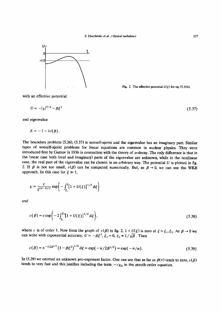
U

0

-1.0


with an effective potential

U = - IxI 4/d - /3~2

and eigenvalue

E = - 1 - iv(/3).

Fig. 2. The effective potential U(£) for eq. (5.31b).

(5.37)

The boundary problem (5.36), (5.37) is nonself-ajoint and the eigenvalue has an imaginary part. Similar types of nonself-ajoint problems for linear equations are common in nuclear physics. They were introduced first by Gamov in 1936 in connection with the theory of a-decay. The only difference is that in the linear case both (real and imaginary) parts of the eigenvalue are unknown, while in the nonlinear case, the real part of the eigenvalue can be chosen in an arbitrary way. The potential U is plotted in fig. 2. If /3 is not too small, v(/3) can be computed numerically. But, as /3 ~ 0, we can use the WKB approach. In this case for ¢ >> 1,

c ) X = ¢ ( d - , , / 2 e x p ( - fe [1 + U(~:)] 1/2 d~

and

(5.38)

where c is of order 1. Now from the graph of v(/3) in fig. 2, 1 + U(s c) is zero at ~ = ~1, ~2. At /3 -~ 0 we can write with exponential accuracy, U = _/3~:2, ~1 = 0, ~2 = 1//~'~ -" Then

U ( f l ) ---- e - 2j°1~1/2 (1 -/3~2) 1/2 de = exp( - rr/2/3 l/u) = e x p ( " x r / a ) . (5.39)

In (5.39) we omitted an unknown pre-exponent factor. One can see that as far as/3(r) tends to zero, v ( f l ) tends to very fast and this justifies including the term -Vgo in the zeroth-order equation.


5.4. The slow time dependence of [3(z)

The equation for the first correction X1 has the form

2 2 / d - 2 2 * • OXO

(5.40)

It is sufficient to study this equation in the region where ~ is order 1, where it can be simplified. In this region one can neglect small t e r m s [3~2.1[" 1 and vx~ and consider X0 as a real function. As a result X1 = - i t , is a pure imaginary function satisfying the equation

a t , - p + x4 /d t , = OXo o -~-~ lJ~ + v([3)Xo. (5.41)

Without loss of accuracy, we can put Xo = Ro. After multiplying (5.41) by R o and integrating one gets the solvability condition

[3t( Rolaxo/a[3) --- - v ([3) ( R 2 ). (5.42)

Now, for ax0/a[3 we have the equation

L ago/a[3 = - ~2Ro, (5.43)

where the operator L is defined in (5.14). Eq. (5.43) belongs to the class (5.19), and we can use (5.20) to obtain

(Rolaxo/afl) = - ½(~2RoIR 1 ) = ( l / d ) ( ~21Ro2 > . (5.44)

We obtain finally

a[3 d( R 2 ) (4.45) a---~ +av([3) = 0 , a = (~2Ro2------- ~ ,

or to within our limits of accuracy,

aot a e x p ( - a t / a ) . a--~- = - X (5.46)

The function a(~') has sophisticated asymptotics r ---, oo. It turns out that the first term of its asymptotic behavior does not depend on pre-exponent factor in v(fl). Actually as r ~ oo,

1 a = "rr In r . . . . (5.47)

S. Dyachenko et al. /Opt ica l turbulence 139

Note a~ << a 2 in agreement with our previous assumptions. From (5.26), we find

g=goexp( l f " ds 1 J l n s J '

AS "r --* ~,

In r ~ In In g + . . . .

Now, from (5.22),

t o _ t = f~d~.g-2= 5~gl - 2 1 n ( l n g ) , (5.49)

so that

~ ( t 0 - t ) In In . (5.50)

Eq. (5.50) was independently derived by Fraiman [19] and by Papanicolau, Sulem, Sulem, Landman and LeMesurier [20, 21]. This was truly an impressive result, which had defied resolution for more than seventeen years. Numerical experiments give a satisfactory confirmation of the behavior (5.50).

So we have shown that structure of collapse in the region ~ ~ 1 is close to a compressing soliton. This region is the most inner zone of the collapse domain. The next zone occurs for 1 >> ~ >> 1/¢1 and is described by WKB formula (5.38). In the next region,

1 >> ~: >> ~:max(~') >> g, (5.51)

and the WKB approach could be used again. The result should be formulated more conveniently for the function ¢, where

~ U l / 2 ~ - d / 2 + c / c t - i / a . (5.52)

The formula (5.52) is correct up to some ~:max(~') that is still unknown. We would conjecture that in the outer region

~max < ~ < g

the collapse will create some kind of integrable singularity.

5. 5. The dependence of the number of particles absorbed per collapse on damping

The central question of interest to us here is the amount of power absorbed in collapsing event. Let us first work this out in the case of the nonlinear dissipation. We have seen that the equation determining

OXo ) d- 2Eg2,+2 f~R~o l O--(°~[R2 2/3R° Yff -'o OtJo [ 0 + e ld~ := -

1 4 0 S. Dyachenko et al. / Optical turbulence

the evolution of /3 = g**/4g is (5.45). We now ask how this equation is modified with the inclusion of nonlinear damping. The easiest way to derive this is to use the exact conservation law

0 t f I¢'12 d r = - 2,f1¢1 "+''/a+2 dr . (5.53)

Now, assuming that the collapse has attained its self-similar shape before the damping sets in and thereby replacing ¢(x, t) by (5.21) and (5.27) with Xo(/3) as Xo(O) +/3 aXo/O/3 where Xo(O) = R o, we find

+s)/d+2ed- 1 de. (5.54)

fgowe de = 1 R o R l e d + , d e =

But

and defining

b = f~Ro~l+s)/d+2~d-1 d~ f ~ R 2 e d+l de '

we obtain, using g-2 a/Ot = 0/0r, and adding the combination for v ( / 3 ) ,

0/3 1 g~, 07 +av(fl)+ebg2*=O, /3= 4 g

The total loss of particle number per collapse is given by

where the dissipation rate

F= - ~---i fl~b[Z dr= 2E fl~bl4<l+s)/d+2 dr=cEbg 2"+2,

oo 2 d + l where c =(20o/d)f~Roe d~ r, with /20 = 1 if d= 1, Do =2~r if Therefore

oo

AN= c f ,bg * dr ,

(5.55)

(5.56)

(5.57)

d = 2 , and 120=4~r

(5.58)

if d = 3 .

(5.59)

where g is obtained by solving (5.56). Now, recall that the relation between t and r is given by (5.22). Observe that if g = [2/3o1/4(t0 - t)~/2] - 1, that in terms of r,

exp(2/3o1/2r) 1 (5.60) g=go /3ol/4 , go = 2to1/2,


if we choose to have t = 0 correspond to r --- 0. To calculate the dissipation AN, we must calculate g(~-) from (5.56). However, no significant dissipation occurs until a time r 0 when Eg 2s becomes of equal size to the other terms in (5.56). Up to that time, the balance in (5.56) involves the first two terms only and this solution we have already discussed. A very important feature is that after a long time, the rate of change of /3 and a is very small. Indeed for (5.47),

g~ 1 (5.61) a = g rr I n r "

Therefore, if we wait until the time r o when eg 2s is of order/3, , the subsequent rates of change of a and /3 occur on the time scale given by

- - r r l n % .

Let

"/" ~ 'tO +/d, Or.

Then, set

/3 = (1/ /z2)B,

and find

(5.62)

and

(5.63)

a = (1//.Q A (5.64)

1 B , ~ + a exp( "rrp, expf j °/z +°'4sB1/2 dcr / z3 2 B 1/2 ) + ~l /2~g2S B s/2 = 0, (5.65)

f= expf~°/~'+~(4sB1/zd{r') AN = ].L3/2c ~g2S B s/2 d~r. (5.66) - - o o

Now, until exp(fffo4s/31/2dr) is sufficiently large to balance (1/#3)B~, and a exN~rl.~/2Bl/2), no significant dissipation occurs. Therefore we choose 3(r) and B(o-) to solve

f l~+av(/3)=O, 0 <~- < r 0 ,

and then choose r 0 such that

(j:0 )1 /x~/2e exp 4sl/~- dt / /3 '

in which case (we can now start calculating dissipation from cr = 0)

A N = --~Cjo -~7-~exp 4sB1/2dcr' do"

(5.67)

(5.68)

142

and

B~ + p,3a exp (

where

g , ~ - 4 B g = O


2B t /2 + bg 2s = 0, (5.69)

(5.70)

and g behaves as go exp( f~ 4sB1/2 d t r ) / B l / 4 near cr = 0. We can verify numerically that B never goes

through zero but tends asymptotically to a new constant which is almost independent o f / ~ and • since t x 3 e x p ( - w l x / 2 B 1/2) ~ 0 as /x ~ oe. F rom (5.68), we obtain to leading order that

1 "Co '~1~6"s~'/2 l n E - I + "'" (5.71)

and therefore

1 1

"rr In In e - , + . . . , (5.72)

and

1 1 A N ~ p---5 ~ ,rr2(lnln _1)2" (5.73)

Observe that if the term v(/3), which causes the ln ln behavior, is absent, then there is no need to

in t roduce the time scale as we did in (5.62) a n d / ~ is arbitrary and independent of e. In that case, A N is

Percentage of burned N 14 , , , , , , , , , , , , ,

13

12

11

10

200 900 1600 kd

Fig. 3. Percentage of burned out energy AN(kd)/N o in 1D single collapse event for damping 3'k = ½k2h(k/ko) •

Inverse burned energy amount 0.106 . . . . . . . . . . . . . .

0.100 ' ~

0.094 /

/+ 0.088 /

/ 0.082 / ~

0.076 /

0 . 0 7 0 . . . . . . . . . 1.70 . . 2.00

log log kd

Fig. 4. Inverse amount of burned out energy 1/AN(k d) in 1D single collapse event as a function of log(logk d) for damping Yk = ½k2h(k/kd ).


E independent but of course, as we have emphasized, it is the presence of v(13) that allows the localized

solutions exist in the first place. Similar arguments give us the parallel result that in the case where we choose the damping to be linear

and concentrated wavenumbers k > k a,

1 (5 .74) AN ~ lnln k d "

This result is directly confirmed by numerical experiment (see figs. 3 and 4).

6. Numer ica l integrat ion s c h e m e

We now describe the procedure used to simulate the solution of the NLS equation (6.1) in the presence of linear amplification and damping, nonlinear damping (due to muliphoton absorption) and parametric forcing. The results we report in this paper do not include the last two. The equation is

ig', + V 2 1 / r --I- a l ~ [ 4 / d ~ + i g g r + i/31~12m~ = A q t* e -2ixt. (6.1)

The two most important considerations when choosing an integration algorithm are that, in the absence of external forces, the constants of motion N, H and P are conserved and that we obtain a reliable description of the collapsing cavity when it is in its self-similar regime and its width is very small. The last point is very important because it is in the small scales where dissipation takes place that the greatest errors can occur. The source of these errors is aliasing. Power is transferred to higher harmonics through the cubic nonlinearity and thus mistakenly deposited in lower harmonics due to the inability of the grid to distinguish between the wavenumbers above and below 1 ~km, where k m is equal to the number of points used to resolve either of the spatial directions x and y. We take - 7 < x < "rr, -'n" < y < w and stepsize A so that k m = w/A and we usually took this to be 128. To overcome the aliasing error, we

I < 1 1 - - ~km, Ikyl > ~k m. divide our wavenumber grid into two regimes: R, ~k m _ k~, ky < ~km, and Ra, Ikxl >- 1

At each time step t, we calculate ~ ( k , t) and V(r , t) and then 1~12~/, in real space and then its value

(1~'12~/,) in wavenumber space on R u R a. The region R contains the true harmonics and the region R a the aliasing harmonics. In calculating the updated value of qt(k, t), we exclude the region R a. Of course, ignoring three-quarters of the information on the grid reduces accuracy but it is necessary. Otherwise, we overestimate the amount of power lost in each collapse event.

The algorithm we use for the pure NLS equation (9 ---/3 = A = 0) is

_ 112 i%n12 n÷l .~.~+, ~.~ V 2 + ~ i~.,+ + +~ .n 0, (6.2) I + "l- O/ = r 2 2 2

where z is the time step, the index j = (j , jy) refers to the grid point x =j ,A, y =jyA, - k m <JxJy < kin, and the index n refers to the time step. V2~. n means the inverse Fourier transform of - k E ~ k where k(k , , ky) is the index denoting points on the grid in wavevector space. It is easy to show that

N = A 2 E I~." + 112 = A 2 E [~n[2 (6 .3) J J


and

H = 4"rr2~k21~ff+'12 '_ a 2 ~ ' ~ l , / , n + l l 4 n 4 2ttza L.,I~rj I =4'rr2y',k2lRff/~l 2 1 2 - - I •

k j k j (6.4)

To prove (6.3), multiply (6.2) by (~."+~ + ~.~)* and subtract from the expression obtained its complex conjugate. To prove (6.4), multiply (6.2) by ( q , , + l _ q,~). and add to this expression its complex conjugate. The linear damping and amplification terms iF" ~ are written in wavevector space as 13'k~(1/.1/~. l ^n +1 + ~ ) where yk = 3'0 + 3',, + 3'd, where 3'0, 3'd are damping terms and 3'p is an amplification. Formulas are given in the next sections by eqs. (7.4)-(7.6). The nonlinear damping term which represents multiphoton absorption in the optical context is written as

i/3 [~ jn+ l [2m+2 _ i1//jnl2m+2 1/_/in+ 1 + ~jn

m + 1 i~-+~12_ i~.12 2

1a¢~*"+1 ~*~). One finds (for m 2) and the parametric forcing term is written as ~ , . j + =

Nn+l _ N n + ½AA2E R e ( ~ , + l + ~.n) im(l/~jn+l + ~.n)

7 J

+ 1/3A2 E (pt/tjn+ 114 + lqtn+ll2l~.nl 2 + I~nl4)l~. n+l + qtj~12

J

+2~r2 E Yk .~..+ 1~. / , + ~ l z = 0, k

(6.5)

and a similar but much more complicated expression for H "÷1 - H " . In the limits of small A, /3 and ~, both quantities are conserved.

We solve the nonlinear implicit algorithm for ~n +~ iteratively as

l t t n + l , s + l ~ n V2~,tn+l,s+l..]_~tn i~ .+ l ,q2 + i~nl z ~n+l,~ + ~ " + + a + D ( q t " + l ' s , q t " ) = 0 1 r 2 2 2

(6.6)

for s = 0, 1 . . . . , cr where ~r is that value of s for which IN n+l'~+l - Nn+Lq is first less than 10-TNL We call ~ + 1 , 0 = qt~ and ~n+l ,~ = ~ .÷1 . The quantity D in (6.6) stands for all the damping, amplification and parametric forcing terms. Notice that both D and the nonlinear term ,~l,/t12,/z are evaluated at the previous iterate. To solve (6.6)we proceed as follows. Start with ~ff and ~ + 1,0 with k belonging to R. Find ~ and ~.n ÷ 1,0 and compute D and the nonlinear terms. Take their Fourier transform. Because of nonlinearity, there will be nonzero contributions for k belonging to R a. Ignore them and solve the linear equation (6.6) for ~ff+ 1,1 for k belonging to R only. Repeat a until s = or. We now have kk~ +1 and l~jn + 1.

Convergence of the iterative procedure requires an upper bound on the time step r. For the moment, ignore D and subtract (6.6) from (6.2) and expand the nonlinear term near ~ . We obtain

(2i ) T -{-V2 (lI~n+l--ltln+l's+l) + 2 l ~ " l Z ( ~ n + ' - ~ n + " s ) + ~ , z ( q , , + , - ~ " + " s ) * = 0 ,


from which we can show that the L 2 norm of ( ~ n + l _ qtn+l.s+l) obeys

I I~ ,+ l _ q,-+l.s+lll _< 3maxlqt"12rllq t n + l - q,-+l.Sll.

Convergence requires

2 r < = z~. (6.7)

3maxl~n[ 2

When the extra terms are added, this Criterion must be slightly modified; for example, the inclusion of 1 parametr ic forcing requires us to add [hi to the denominator of ~'¢. We chose ~- = 3r and found that it

takes about six to eight iterations to converge to the chosen accuracy. Observe that near a collapse, z c becomes very small indeed.

7. D i scuss ion o f results

We now present the results of numerical simulations in the two-dimensional case. As we have pointed out already, this case is difficult because none of the simpler kinds of stationary solutions obtain and in particular we cannot obtain a pure Kolmogorov spectrum in either the left or right transparency window. On the left, the sign of the flux Q is negative for the pure Kolmogorov spectrum (3.21) because 3' = - 1 lies in the interval for which - ] I ' ( x l ) in (3.23) is negative. To remedy this problem, we then introduced the finite tempera ture Kolmogorov solution (3.39) and ~b(to) given by (3.46), so that

T n = _ , _ _ _, (7.1)

tz + to + atdT-3to2lln( to/toc)J 2 "

We emphasize that this solution cannot hold everywhere on the frequency axis 0 < to < oo because the correction is not everywhere small. Nevertheless, as we show in figs. 5, 6, and 7, it does seem to hold very

well in the left t ransparency window to2 < to < too, where the correction is small with respect to the thermodynamic background.

Such a solution is not unreasonable. Recall that the reason for the failure of the thermodynamic equilibrium solution is that it does not allow the energy to tend to zero, as it must because of finite damping, as to-~ oo. However, the left transparency window is shielded from the energy sink by the source of new particles and energy at to = too. However, we cannot expect a pure thermodynamic equilibrium because of the necessity for a finite flux of particles towards to = 0. Hence the compromise solution (7.1). We find that (7.1) fits the data very well for both the focusing and defocusing values of a w h e n / z = 400, T = 10, and aQ = 0.25 and toc = 1 over the broad frequency range 60 < to < 4100.

In our simulations, the amplification and damping components of the coefficient 3"(k)= 3"p(k)+ 3'd(k) + 3"o(k) were given by

yp (k ) = - ~ [ ( k 2 - 602)(622 - k2)] 1/2,

= 0 ,

3'd(k) = O .5k2h(k /kd ) ,

60 < k < 62,

0 < k <60 , k > 6 2 , (7.2)

(7.3)


-8 c -

v O , I

o -12

Negative nonlinearity, t = 53.85 - 4 i i i n l i i

6 log 2 (k)

t --4

"-t -'4

-4

6 7

Fig. 5. Time averaged stationary spectrum I~bk[ 2 for run A (a = - 1 with strong damping at k = 0) and theoretical prediction for 2D spectrum (7.1) with T = 10,/~ = 400, to c = 1, aQ = 0.25.

-4

-8 c -

O -12

-16

Positive nonlinearity, t = 30.20

0 1 2 3 4 5 6 7 log 2 (k)

Fig. 6. The same as in fig. 5, but for run B (t~ = + 1 with strong damping at k= 0).

~ --8

.9o -12

Negative nonlinearity, t = 41.53

-16_, 6 g 7 log 2 (k)

Fig. 7. The same as in fig. 5, but for run C ( a = +1 with no damping at k = 0).

whe re

1 1 e5[l_(1/x2)] h ( x ) = ~ ~-g , x < l ,

5 ~ l / 2 ( I - - x 2) = l - g ~ , x > l ,

and

3 '0(k) = 20(~k - 1) 2, k < 6,

= 0, k > 6. (7 .4)

The mot iva t ion for these choices was as follows: 3'p(k) is the l inear growth ra te of the p a r a m e t r i c

instabi l i ty for spin waves in fe r romagnet ics , yd(k) mode l s the l inear L a n d a u d a m p i n g in p lasmas , and

y o ( k ) is chosen to cont ro l the growth of the co nde nsa t e at k = 0. T h e s tudy was ca r r i ed ou t in the case of

weak instabil i ty, i.e. 3"p/k 2 ~ 10 -3.

Al l s imula t ions were in i t ia l ized by a field ~k(0) of small r a n d o m noise. In figs. 5, 6, 7, we show the left

t r anspa rency window 60 < ~o < 4100, for t h r ee cases, a = - 1, o~ = + 1 with s t rong da mp ing at the origin

and a = + 1 wi th no damp ing at the origin, wi th the s p e c t r u m (7.1) supe rposed . T h e s e g raphs were

o b t a i n e d by averaging the ca lcu la t ed d a t a ~k for a fixed va lue of k = Ikl first over angle by tak ing ~k at

kj = k[eos ¼n~, sin ¼n~r], n - 0 . . . . . 7 and t hen over a t ime interval app rox ima te ly t en t imes the p e r i o d of

the lowest u n d a m p e d m o d e k = 6. Observe tha t all spec t ra a re app rox ima te ly the same and fit the

theore t i ca l curve (7.1) very well. W h a t is ev ident is tha t the p re sence of in ter rn i t tency and co l lapses does

not affect the weak tu rbu lence spec t rum in any subs tan t ia l way. Never the les s the i r p r e sence is seen

vividly when we examine the par t i c le n u m b e r d iss ipa t ion

K'(t) = f ,kl%l 2 dk (7.5)

for the same th ree cases a = - 1 (defocusing) , a = + 1 (3'o present ) , a = + 1 (3'o = O) (see figs. 8, 9 and

Dissipation rate 800 . . . . . . . . . . . . 600 400 200

0 -200 --400 -600

-800 I I I I I I = = J I I t

-1000 50 51 52 53 54 55 56 Time

Fig. 8. F(t)=fyklOkj2dk in the stationary state for run A.


i4oo 2000 1800 1400

1000 600 200

-208 --60(

-100(

Dissipation rate I I I I I I I I

I I I I I I I I

28 29 30 31 Time

Fig. 9. The same as in fig. 8, but for run B.

147

400O

3000

2000

1000

0

-500

Dissipation rate

39.6 40.2' 4().8' '41.4' '42.0 Time

Fig. 10. The same as in fig. 8, but for run C. Note the difference in scale from fig. 8.

10). Because we include contr ibut ions f rom all k values including the ne ighborhood of k -- k 0 where Yk is negative, F ( t ) takes on positive and negat ive values. In the last case, because of no damping at k = 0, the uns table condensa te tr ies but is unable to form due to the modula t iona l instability and a sequence of collapsing f i laments occur at r a n d o m points in space and t ime. Al though they Carry little energy to high wavenumber s ( the value of H for a collapsing f i lament is approx imate ly zero i see section 5), they do carry part icle n u m b e r and deposi t it as shown in fig. 10. Not ice the difference inlscales f rom figs. 8 and 9.

The dissipation rate measu re s the flux of part icles towards high wavenumber s and frequencies . R e m e m - ber this does not violate our a rgumen t tha t a flux of energy towards to = ~ must be accompan ied by a flux of part icles towards to = 0. This a rgumen t is valid for the case of weak turbulence when E k -- tokn~, namely when the principal contr ibut ion to H is f rom its kinetic energy par t fJVgrl 2 dr . But for the strongly nonl inear collapse, the potent ia l energy c o m p o n e n t - f½1~l 4 d r is large and ba lances the kinetic energy so that the energy carr ied by the nonl inear pulse is zero. In such a situation, there is no contradic t ion in having a negat ive Q or a r ightward flux of particles.

W h e n there is s t rong damping at the origin, the n u m b e r of part icles f luctuates weakly as is shown in figs. 11 and 12. T h e reason for this is that the gain-loss history of a part icle in the left t r ansparency window is out of phase with the gain-loss of part icles in the damping window nea r k = 0. One can

N(t) N(t)

3000 ~ ' ~ ' ' ' J " ' ~ l 2800 . . . . . . . .

2200 I- 20oo I- . . . . . . . . 1 50 51 52 53 54 55 56 27 28 29 30 31

Time Time

Fig. 11. Time-evolution of N(t)= fil l 2 dr in the stationary state for run A.

Fig. 12. The same as in fig. 11, but for run B.

N(t)

I ............. 1 2400 ~ _

2000 I

1600 / . . . . . . . . . . . . . 39.6 40.2 40 .8 41.4 42.0

Time

Fig. 13. The same as in fig. 11, but for run C.

= . 1


( b ) t = 3 4 . 3 3 5 9

Fig. 14. Snapshots of one collapsing cavity on the weak- turbulent background. (a) Beginning of collapse, (b) peak, (c) end of collapse.

roughly model the situations as follows. Let nw be a typical particle number density in the window and let n 2 be a typical particle density near k -- 0. The former gains primarily through a nonlinear field from the neighborhood of k 0 proportional to n 2 n , and loses through a nonlinear interaction - n w n 2. On the other hand, particles are lost a t k 2 through linear damping 3'0 and gain through a nonlinear interaction nwn2 . 2 Write n 2 = , 3 ' o n 2 + nwn2 , 2 n w = 3"n w - nw n2 ", = d / d t , and we obtain the classical p reda to r -p rey

2 model. The equilibrium n w -- 3'0, n2 = 3' is a center about which there are periodic orbits with periods 2at ~-y0~, which is the behavior we observe. On the other hand, in fig. 13, the presence of many collapses changes the picture so that there is a strong and immediate feedback from n 2 to nw and, as a result, no oscillations are seen.

In fig. 14 we show a single collapse in three stages of its life. Observe how large the fluctuations are with respect to the weak turbulence background so that one can expect the tails of the almost Gaussian distributions to be lifted if there are many of these events. As a measure of the effects of the collapses on the weak turbulence background, we measured the fourth-order correlation in Fourier space

Q O ) ( k l , k z , k 3 , k4)=im_~]r l r ~k~k~aIt~,*~, * d t , k 1 + k z = k 3 + k 4 , ($1SzS3S4) ~/z Jt J 0

(7.6)


Negative nonlinearity 0.040 . . . . . . . . .

0.030

o. ~" 0.020 o

0.010 ~ !

I I I

010 0 10 P

Fig. 15. Imaginary part of fourth-order correlation function for run A.

Positive nonlinearity 0.040 . . . . . . . .

A~ 0.030

~" 0.020 0

0.010

I I I I I

10 0 10 P

Fig. 16. Imaginary part of fourth-order correlation function for run C.

where

1 T ^ 2

and

k 1 = ( 2 0 , 0 ) , k 2 = ( - 2 0 , 0 ), k 3 = ( O , 2 0 - p ) , k4 = (O, - 2 0 + p ) .

I f weak turbulence dominates, we expect this function to be nonzero. Only in the vicinity of a resonance

kl + k2 = k3 + k4, °31 + °32 -- °33 + 034 where 03k = oJk +/~k the (slightly) amplitude modified frequency. We note that when a = - 1, there is indeed a peak at p = - 1 (see fig. 15). The presence of collapses acts like a perturbat ion of the double spectrum (a single frequency oJ has two free travelling waves e ± ~ x - i , o t ) and splits the resonance to p = - 5 and + 1 (see fig. 16). In a manner we do not yet know

how to interpret, the Gaussian nature of the weak turbulence theory is slightly modified by the occurrence of collapse events obeying a Poisson distribution.

8 . C o n c l u s i o n

In this paper, we have presented the weak turbulent theory of a class of Hamiltonian systems of nonlinear Schr6dinger type and discussed the relevance of various equilibrium states. Our main attention has been directed to the stationary situation where a balance is achieved between the input of particle number and energy in a narrow window of intermediate wavenumbers (k 0 - Ak, k 0 + Ak) and the losses of particle number and energy through damping at the origin k = 0 and infinity k = oo respectively. One of our main points has been that the conservation of energy and particle number in the ranges of wavenumbers (0, k 0 - Ak) and (k 0 + Ak, ~) means that as energy density flows: towards high wavenum- bets, particle density flows towards low wavenumbers. The consequences o f the buildup of particle number near k = 0 are nontrivial and lead either to the formation of condensates in the defocusing


(a = - 1) case or to collapsing filaments in the focusing (a = + 1) case. In the former.case, it is necessary to introduce damping at k = 0 in order to control the amplitude of the condensate. In the latter case, because the condensate is unstable it is never reached. Instead, collapsing filaments are formed which reverse the flux of particle number and induce a secondary flow which carries particles to high wavenumbers. No damping at k = 0 is required.

The primary flows of energy and particle number density were described by weak turbulence theory in which the transfer of spectral densities are achieved by four-wave resonant interactions. The interactions are local in the sense that the transfer functions st(n, n, n) exists for classes of solutions nk in the neighborhood of the Kolmogorov spectra. Because all nonresonant interactions are ignored, statistical information is lost, and the solutions depend only on the values of the particle number and energy density fluxes and parameters T and ~, which we identify as temperature and chemical potential. For the primary fluxes, all the usual Kolmogorov assumptions made in the context of hydrodynamic turbulence, and listed below, are valid. In the secondary flux of particle number density, however, things are radically different. The flow in wavenumber space is simply the manifestation of a collapsing filament in physical space in which number density is squeezed from large scales to small scales in a highly organized and coherent manner. No statistical information is lost. Statistical considerations are introduced by the intermittent nature of these events, the uncertainty in time and space as to when and where they occur. They are in all likelihood, governed by a Poisson statistics whose parameters depend on the flux of particle number towards the origin. Because the events involve large amplitude fluctuations, their impact on the probability density function of the field ~ ( r , t) is to cause an elevation in the tails of the distribution. In the remainder of this conclusion, we will argue that this mechanism for intermittency consisting of (i) an inverse cascade associated with the spectral density of an additional finite flux motion invariant, leading to (ii) a continuous formation of large-scale structures which (iii) are intrinsically unstable to a broadband spectrum of perturbing modes which directly and quickly transfer power or energy back to the small dissipative scales, in some cases through highly organized, collapsing solutions, may have broad applications. In particular, we will look at its possible relevance for three-dimensional

hydrodynamics. Before we begin, we want to note some important similarities and differences between two-dimen-

sional optical turbulence and practical manifestations of three-dimensional hydrodynamical turbulence. In optical turbulence, there are situations in which it is reasonable to assume that number and energy density production occurs at scales intermediate between the dissipation scales and overall box size. As long as the ratio of the pumping rate Y0 to the insertion frequency too is small, weak turbulence theory obtains to a good approximation and there is room for the resulting inverse cascade. Since collapsing filaments follow from a modulational instability which is most easily triggered when the spectral number density has condensed at a single wavenumber, and in an infinite geometry this wavenumber is k - 0, damping at small wavenumbers, as we have shown (cf. compare figs. 9 and 10), severely inhibits intermittency. If the box size were finite of linear dimension L and small enough that 2"rrL - 1 ~ k 0, intermittency would still be present because of the tendency of the spectral number density to condense at the smallest wavenumber available to the system. Collapses would form and there would be direct cascades of both energy and number density towards k = o,. Indeed, even if L >> 2wk o l, as the pumping rate is increased so that the ratio y0/to0 approaches unity, the rapid growth of N, the average particle number, would mean collapses would form long before weak turbulence theory had a chance to come into play and build an inverse cascade. In that case, too, number density and energy would exhibit direct cascades. Intermittency effects would be large and in all likelihood overcome any relaxation to a

Kolmogorov-like spectrum.


The appearance of a good approximation to the Kolmogorov spectrum at high wavenumbers means that, in some sense, three-dimensional hydrodynamics is more like the weak turbulence case with a small frequency of collapses. However, in that context, we are usually dealing with (a) decaying turbulence or (b) turbulence created, usually through instabilities, at scales 2"rrko ~ of the same order as the box size. For (b), the integral scale of the turbulence, the length scale corresponding to the wavenumber at which the spectral energy E(k) is maximum, is the box size. In this case, there will not be any inverse flux from k 0 to smaller wavenumbers because there are none available to the system. Any intermittency which occurs comes from collapsing filaments which arise from large-scale structures at the scale 2 ~ k o ~ which are either directly forced or else are built through an inverse cascade of the spectral density of the second motion invariant from wavenumbers k such that k 0 << k << k d. We remark that just because energy is inserted into the system at k 0 does not mean that the instabilities which introduce this energy also produce the type of large-scale structure susceptible to fast instabilities of the collapsing filament type. Furthermore, an increase in box size beyond the integral scale could leave room for an inverse cascade and an increase in the frequency of events which lead to intermittency. It is quite possible that this increase would never reach the point where one loses the Kolmogorov spectrum altogether and so, in this sense, one might say that the behavior at small scales is independent of box size. Nevertheless, the convergence to the Kolmogorov picture would be less uniform in the higher order moments.

Therefore, although the inverse cascade may not be the only mechanism to produce the structures which give rise to intermittent collapses, there is no doubt that it can play some role. We will show that if the spectral density of squared angular momentum is produced at a constant rate at some intermediate wavenumber, then only a finite amount can reside in small scales and the rest must be reassigned to large scales. Further, we suggest that this spectral density has the right character to~ produce the large-scale structures (the analog of the condensate in optical turbulence) which can lead to collapsing filaments. There is some experimental evidence that the incomplete burnout or dissipation of the filaments themselves also give rise to larger scale eddies in the hydrodynamic context. Douady, Couder and Brachet [22], using a new bubble visualization technique, observe that the short-lived high vorticity filaments, which appear to form spontaneously, disintegrate through helical instabilities which stir large eddies. In what follows, we simply discuss a plausible scenario, motivated by our observations in optical turbulence. Direct verification of the role of an inverse cascade will probably have to await a more complete understanding of the nature of the instabilities which result in intermittent events.

Kolmogorov [12] proposed a universal theory for small-scale eddies in high Reynolds number turbulent flows. It rests on several assumptions, that the transfer of spectral energy to large wavenumberS is local over a window of transparency (the inertial range) in wavenumber space, that :statistical information is lost in the cascade so that average flow quantities are scale invariant and determined by the mean rate of energy flux e, which is constant in a statistically steady state. If E(k) is the spectral energy (u --~ = rE(k)dk) then, for isotropic turbulence, the equation for E(k) is

aE( k) = T(k ) - 2 v k 2 E ( k ) + f ( k ) , Ot (8.1)

where T(k) is the energy transfer integral given by a linear functional of the third-order moment in velocities. It is called a transfer integral because it neither produces nor dissipates energy and it has the property that fT ( k )dk = 0. The terms f (k ) and - 2 v k 2 E ( k ) represent the prodUction and dissipation of energy. The former could be proportional to E(k) if energy is introduced by an instability process, but we assume that its domain of support is confined to a narrow window. Between the range of


wavenumbers (k 0 - Ak, k 0 + Ak), at which energy is produced, and the dissipation range R a = (Ev-3) 1/4, where the -2vk2E(k) term is important, we assume there exists a window of transparency, the inertial range, where both f (k) and - 2 v k 2E(k) can be ignored. In this range, we assume the turbulence relaxes to a stationary state E t --- T(k) = 0, but we will also assume that, in the neighborhood of the solutions which realize this state, T(k) exists. This means that the interactions are local in the sense that the integrand of T(k) (T(k) is an integral over a third-order moment) must decay sufficiently fast as Ik' - k I; k', the integration variable, becomes large so that the integral exists. In the absence of dissipation and forcing, (8.1) has conservation law form E t = T(k)= -P'(k) , where P(k) is the energy flux, positive when the flow of energy is to small scales and large wavenumbers. We remind the reader that we call fbE(k)dk (usually a = 0, b = oo) a true constant of the motion if P(k) = 0 at both k = a and k = b, so that the total energy is trapped in the interval (a, b) for all time because of zero flux through the boundaries. However, the presence of viscosity makes these thermodynamic equilibria uninteresting because there is a constant leakage of energy through to the dissipation scales. Therefore, in any interval (a, b) of the transparency window where a > k 0, b < k d, a(ffE(k)dk)/Ot is zero by virtue of the fact that the fluxes P(k) at k = a and k = b are not zero but the same. In this case, we call fabE(k)dk a finite flux constant of the motion. In this paper, it is the finite flux constants which are important. Moreover, within the window of transparency, the interval (a, b) is arbitrary, so that then P(k) is a constant and equal to the mean dissipation rate e throughout the inertial range. From dimensional considerations E(k)(13t-2), k(1-1) and e(lZt -3) are related by the well-known Kolmogorov law E(k)= c2e2/3k -5/3, where c 2 is a universal constant. The relevance of such solutions to turbulence rests on the Kolmogorov assumption that the energy dissipation rate e = - d ( u 2 ) / d t = 2vfk2E(k)dk does indeed settle down to a steady state value in which the energy production rate f f (k)dk is balanced by the dissipation rate.

What quantity or quantities in hydrodynamics can play the role of the additional finite flux motion invariant? We will consider only the isotropic case and define the velocity correlations

u--~(r) = (u(x) u(x + r ) ) = fo=F(k) cos (kr ) dk (8.2)

and

~ 3 / 2 h ( r ) = ( v 2 ( x ) u(x + r ) ) = fkH(/¢) s in(kr) dk , (8.3)

where u and v are the velocity components parallel and perpendicular respectively to r and U'-'~= 1 3 2 ~Ei=l (u i (x) ) = E , where E is the total energy. The Von Karman-Kowarth equation for the

velocity correlation f(r) is

1 2vh--~l 8 4Of ~--[u--~f(r)+ 2~23/2-- -~ -~r -~. (8.4)

We have not included in (8.4) any forcing terms. From (8.4), we obtain formally

U2"I - l i m 2 ~ 3 / 2 - r4h(r) = - 2 v = - e , r--*0 F 4

~t ..~ 1 a 4af 1 0 r4h(r) - 2 v u l i m - - ~ - - r - ¢ - , (8.6) u--;2)i~m® raf(r) + r--~c~lim 2 ~ 3/2 r i~r r - - *ov r or or


and

-~u 2 r 4 f ( r ) d r + 2 u [ r h(r) l 0 = 2 v ~ r 4 0" (8.7)

In (8.5)-(8.7), we have used the facts that as r --> 0 (k is the Taylor microscale [ - f " ( 0 ) ] - 1/2),

f ( r ) ---, 1 - r 2 / 2 A 2, h ( r ) = # ' ( r 3 ) . (8.8)

In the absence of viscosity, eq. (8.5) expresses the conservation of energy. In the presence of forcing at intermediate scales ko 1 and under the assumption that viscosity acts only after the viscous scales k~ 1, the Kolmogorov assumptions assert that the turbulence relaxes to a steady state for which the dissipation rate e is constant, and moreover that it is the only relevant parameter besides the local scale k-1 in determining the statistical behavior in the wavenumber window (k0, k d = ( 8 1 ) - 3 ) 1 / 4 ) . Eq. (8.6) could be trivial if

m

M = lim u2r3f (r ) (8.9) r . - . . o o

is zero. If, however, M is nonzero, then it has the additional consequence that the quantity, whose time derivative is given by (8.7),

L = fo®-~rnf(u) dr (8.10)

does not exist. In this case, eq. (8.7) requires interpretation. If M is nonzero, then in (8.6), the viscous term involving (1 /r ) (O/ar)r4Of/ar tends to zero as r---> oo and so if h ( r ) = d~(r -3) as r ~ 0% M is a motion invariant,

aM~at = 0. (8.11)

On the other hand, if M = 0 and h(r) ~ cr -4 as r ~ oo (see ref. [21]), L exists and is almost a motion invariant,

OL /Ot = - 2 ~ 3/2C = - - / d , . (8.12)

The quantity L is called Loitsyanskii's invariant and represents a measure of squared angular momentum

4 w L = fr2(u(x) u(x + r)) dr. (8.13)

Its existence was established by Batchelor and Proudman [23] under the assumption that at some initial moment in time the turbulent field haS convergent integral moments of the velocity distribution. These authors showed that under similar conditions, the third-order velocity condition h(r) does not decay sufficiently fast so that L is constant but found that h ( r ) ~ cr -4 as r ~ 0% which leads to (8.12). Nevertheless, we shall argue that in the case where L exists, L is a finite flux motion invariant in exactly the same way that the energy E is and that its loss occurs at low wavenumbers near k = 0. We shall show


that if the fluid is continuously stirred at intermediate scales ko I, then the energy density E(k) (E = fE(k)dk) flows to high wavenumbers at constant rate e and the squared angular momentum density J(k) (L = fJ(k)dk) flows to low wavenumbers at the rate/~.

The quantity

3

fo®( ' f=E( M= l im(r3f(u)) = r3f) d r = (4'rr) -1 ui(x) u i ( x + r ) ) d r r "-~ao i=

(8.14)

corresponds to squared momentum. It is a true motion constant. Its existence and invariance was first noted by Saffman [16]. Saffman argues persuasively that M is not likely in general to be zero and supports his argument by showing that if a turbulent field is generated by a distribution of random impulsive forces with convergent integral moments of cumulants, equivalent to convergent integral moments of the vorticity distribution at the initial time, thus M is nonzero and invariant.

In what follows, we will keep both options open so that when we discuss L we are assuming it exists and that M = 0. To continue our arguments in wavenumber space, we now define spectral densities for L

and M. Consider

. o o _ _ oo

j ( r ) = jr u2r4f(r)dr= f o J ( k ) c ° s ( k r ) d k (8.15)

and

m(r) = L~u-2(r3f(r)) ' dr=M-u--~r3f(r)= f o M ( k ) c o s ( k r ) dk. (8.16)

A little analysis will show that kJ(k) and kM(k) are the Fourier integral sine transformations of u2r4f(r) and u---2(r3f) '. The Fourier integral cosine transforms of these two quantities are respectively B4F(k)/~k 4 and k a3F/Sk 3 - 3a2F/ak 2 and, using the relation

1 [ : O2F a F ) (8.17) e ( k ) = [ k - f f - k - f f

between the one-dimensional Fourier integral cosine transforms F(k) defined by (8.2) and E(k)= 4 2 3 ~ark F-,i= l~ii(k), where

1 f~(ul(x)Um(X "~-r))dr, ¢ ~ l m ( k ) ( 2.T/. ) 3 -

we have k a3F/ak 3 - 3 ~2F/ak 2 is (3k-lE(k)) '. Now Fourier integral cosine C(k) and sine transforms

S(k) are related through Hilbert transforms. (Observe that C(k) and S(k) can be defined by even and odd extensions to negative k, that C(k) + iS(k) is analytic for Im k > 0 and thus the assertion follows

from Cauchy's theorem.) We find (note M = 0 does not imply M(k) = O)

[a4F(k')/ak '4] dk' a4F(k) 1 p f ~ k 'J(k ') dk' kJ(k) = - 1 P [ ~ k'

Ok 4 "IT j_~ -~--Z_-~ , ~r j_~ - k (8.18)


and

0 3 E ( k ) Ok k

From (8.18), we obtain that, for small k,

04F 2 f : 2 L Ok 4 = --~ J ( k ' ) d k ' = vt

so that, integrating (8.20) and using (8.17),

E ( k ) = -~-~k " 4

and for large k ( f F ( k ) d k = f E ( k ) d k = E),

24E k J ( k ) = vrkS.

155

k ' M ( k ' ) dk' 1 b 3 E ( k ' ) 1 P [ ~ k ' k M ( k ) = - 1 P [ ~ k ' d k ' . "rr j ~ - k ' ~r J _ . , k ' - k Ok'

(8.19)

(8.20)

(8.21)

(8.22)

Eq. (8.21) is the well known but often disputed result, that the spectral energy at large scales behaves as k 4. The consequences of (8.22) are nontrivial because it says that the amount of squared angular momentum between k o and oo

fkS j 24E ( k ) dk = 5"rrk-----~ < oo. (8.23)

Therefore if squared angular momentum density J ( k ) is introduced at a constant rate at k 0, only a finite amount can be absorbed in wavenumbers k > k 0 and since, as we will shortly show, there is no squared angular momentum density sink at large wavenumbers, the f lux o f J ( k ) must be to small wavenumbers. From (8.19), we have for small k that

E ( k ) = ( 1 / 6 a r ) M k 2

so that when M is nonzero, the spectrum of E ( k ) near k is thermodynamic. For large k,

(8.24)

M ( k ) = - 6 E / ' r t k 4

so that the amount of squared angular momentum between k 0 and oo is

(8.25)

f~SM( k ) d k = - 2E/~rk3o . (8.26)

Again, we see that if M ( k ) is produced at a constant rate in (k 0 - Ak, k o + Ak), most of it must drift to small wavenumbers and large scales. Unlike squared angular momentum density, however, there is no sink at low wavenumbers to absorb squared momentum density. Therefore, if M ~: 0, any large-scale

156 s. Dyachenko et al. /Optical turbulence

structures produced by the buildup of M(k) at low wavenumbers must be unstable and the instability must be fast enough to return squared momentum to high wavenumbers at its original production rate.

The equations for the spectral densities F(k), M(k ) and J(k), corresponding to (8.5), (8.6) and (8.7)

are

0"-----~-- + T l (k ) = - 2 u k E F + 4 k F d k ,

equivalent to (8.1) by applying the operator ½k z 0 3 / 0 k 2 - l k 0/0k,

(8.27)

and

OM(k) 2v-~ ( ~ 1 0 40f 0"--'-7"--+T2(k)= "~ :o r -~r - ~ c o s ( k r ) d r , (8.28)

OJ(k) 4vu--~f: ~_ 7 Of - - -- r 4 cos (kr )dr , 0t + T3(k) = "rr

where the transfer integrals Tj, j = 1, 2, 3, are

r (k) = 4y 3/2 : = 1 0 7r Jo r 4 - ~ [ r 4 h ( r ) c ° s ( k r ) ] d r '

-- ~r r [r4h(r)] c o s ( k r ) d r ,

and

(8.29)

(8.30)

(8.31)

T3(k) = 4 - ~ 3 / 2 f o ~ [ C - r 4 h ( r ) ] c o s ( k r ) d r . (8.32)

When integrated over k, we obtain (8.10), (8.11), and (8.12). Observe that, in the absence of forcing, the decay of E is caused by the viscous term in (8.27) because f T l ( k ) d k = 0, whereas this term gives no contribution to the decay of L. On the contrary, the decay of L is caused by the large-scale behavior of the third-order velocity correlation due to large-range pressure forces. For example, if we take rnh(r) = c[1 - rE/(r 2 + r 2) + . . . ] then T3(k) = 2cu-'23/28(k) as r 1 --* oo, SO that the dominant behavior in

fT3(k )dk = - / z arises from the neighborhood of k = 0. If we assert t ha t / z is constant and that, just as the dissipation rate e plays an important role in the window of transparency (k o, kd), the squared angular momentum flux rate /x plays an important role in the window of transparency (k~ = ri -~, k0),

then the dimensional considerations lead to the behavior

J( k ) = cltx2/3k- 10/3. (8.33)

We stress that there is no evidence to date that the requisite conditions of locality are satisfied for (8.33) to hold. We also stress, however, that this law is not crucial to our argument that J(k) flows to small

wavenumbers. [At this point, we digress to mention several curious results, the ramifications of which we do yet

attempt to build into the total picture. As we have mentioned in section 1, in the absence of viscosity and helicity, the use of Clebsch variables A,/z (u = AV/z + Vq~, ( D / D t ) (A,/z) = 0, a k = F T ( A 4- i/x)) allows us


to recast the Euler equations in the form (1.14). From this it follows ( a / b t ) f ( a , a ~ ) n d k is zero, n = 1 , . . . , ~. Further, if one uses a Kraichnan direct interaction approximation in (1.14), one obtains a kinetic equation for n k, n k 6 ( k - k I) = ( a k a ~ ) , which formally possesses two Kolmogorov spectra E k ~ k -5/3 and E k ~ k -~. The latter corresponds to a constant flux of the density F n = (aka~) ~ for n = 1 and has the units of angular momentum. For general n, one obtains the spectrum E k ~ k "tn), - 1 < a(n) < 5 where, in the limit n ~ , the exponent a(n) is 5 7, which is exactly what obtains from (8.33), corresponding to a flux of squared angular momentum. It is interesting that the two limiting conservation laws both correspond to situations in which one assumes that the statistics are chiefly dominated by a flux of a functional of angular momentum.]

No matter whether M or L is invariant, we have shown that, if produced at a constant rate at k0, the corresponding spectral density will flow to small scales. The question thus is: what is the fate of these "part ic les"? Do they condense into large scale structures as in the case of defocusing NLS or in two-dimensional hydrodynamics, where mean squared vorticity density flows to small scales and energy to large scales where it builds large vortices? Or do they behave as in the case of the focusing NLS, where instead of building condensates, they nucleate collapsing filaments which return the energy to high wavenumbers?

Our conjecture is that the inverse cascade of J (k ) should lead to the formation of large vortical structures just as the inverse cascade of particle number in NLS should lead to condensates. But in the focusing case, we have seen that because these condensates are unstable, they never get a chance to form. Instead, as soon as the particle number density reaches scales large enough to nucleate collapsing filaments, the latter are formed and the inverse cascade is reversed. We can picture this in phase space as follows. The phase point which represents the state of the system is attracted towards the unstable manifold of the condensate which is a saddle point. So although the condensate itself is never realized, its unstable manifold plays an important role in the dynamics. Likewise, in three-dimensional hydrodynamics, we should look at the instabilities of large vortical structures although these structures themselves will never get the chance to form. We know from the work of Bayly [24] that elliptical vortices are unstable to a subharmonic resonance between the inertial wave e ik(t)'x with frequency to = 21-1 cos 0,

where S2 is the rotation speed of the vortex and cos 0 = ~ . k / O k . The subharmonic resonance occurs at 1 0 = 3rr and the window of instability depends on the amount of ellipicity (u = ~O( - 1 - a)y , / - / (1 - a)x , O)

in the original vortex. The rate of growth of the instability is proportional to a and independent of the wavenumber k and therefore the amount of energy which is inserted directly in short waves is largest because the volume between k and k + dk between the two cones ½~r(1- /3a) < 0 < ½"rr(1 + /3a ) is proportional to k. Therefore, although the lowest energy configuration for a given amount of angular momentum is a circular vortex, the distortion of a single vortex by its neighbors leads to three-dimensional instability. One would expect the net effect of the instability is to restore an isolated elliptical vortex to its circular shape, but the constant flux of squared angular momentum to low wavenumbers keeps producing distorting fields. Again we expect the rate of energy feedback to large wavenumbers through the instability process is directly proportional to the flux of squared angular momentum towards k = 0 .

We remark that if M = 0, the existence of L means that squared angular momentum is j z = p2(f(r × v ) d V ) z is proportional to the fluid volume V (see ref. [25]). I f M 4= 0, then the divergence of L means that the ratio of j z to V tends to infinity as V ~ ~ and that large vortices may be even more important than in the case of finite L.

Finally, if M 4: 0, one should also ask about the fate of squared linear momentum as it reaches large scales. At this time, we have no reasonable scenario to suggest.


Appendix A

We show how to average the Dirac delta functions 6(k - k I - k 2) and 6(k + k I - k 2 - k 3) over angles. First we consider ( 6 ( k - k I - k2)). We find

f 6(k-kl-kE)dOdOldO2=2=f 6 ( k - k , cosO,-kECOSO2)6(klsin01 + k 2 s i n O 2 ) d O l d O 2

4"rr (A.1)

S (2kEg 2 + 2 k 2 k 2 + 2 k ~ k E - k 4 - k ~ - k 4 ) 1/2"

Here

S = I 2 2 2 k 2 k ~ _ _ k 4 _ z ( 2 k kl + 2 k 2 k 2 + - k 4 k24) 1/2

is the area of a triangle with given size lengths, k, k 1, k 2.

Next we consider (t~(k + k 1 - k 2 - k3)). Deno te

f f f f ~(k -.bkl-k2-k3)dOdOldO2dO3=R.

Next, write

where

So,

~(, + k, - k2 - k3) = f ~ ( k + k, - , ) ~(, - k2 - k3) dA

= 2~rf*m"xo(k cos 0 + kl cos kl - A) 6 ( k sin 0 + k I sin 01) Amin

× 6 ( k 2 cos 02 + k 3 cos 03 - A) (k 2 sin 02 + k 3 sin 03) AdA,

/~min = max(Ik - kll, Ik 2 - k31 ),

Area ~ = m i n ( k + k~, k 2 + k3).

n = 211'fAmaxA d , f f ~(k c o s 0 + k, c o s o , - , ) ~(k sin 0 + k, sin 0 , )d0d0 , Amln

× f f ~(k2cosO2 + k3 c o s 0 3 - A ) t ~ ( k 2 sin 0 2 + k3sinO3)dO2d03.

(A.2)

(A.3)

(A:.4)


In each double integral in (A.4), one can change variables of in tegrat ion and get

~a=~x 1 1 A R = 2at - - X d a , J~..~. S1 S2

where S~ and S 2 are the squares of the t r iangle with sides k, k l, A and k 2, k3, A respectively:

21 ,, 1/2 S l = ¼{[ (k + k , ) 2 - a 2 ] [ a 2 - ( k - k , ) ] } , $2 = ¼ { [ ( k 2 + k 3 ) i - A 2 ] [ A 2

T h e r e f o r e R is a comple te elliptic integral of the first kind,

R = 16"rrfa--'" {~t,.,. da2 1 .

159

(A.5)

- ( k2 -k3 )2] } '/2.

(A.6)

Now recall that k 2 + k E = k 2 + k 2. With this condit ion the limits of in tegrat ion in R have two

possibilities, Ami n = Ik 2 - k31 , )tma x = k z + k3, or Ami n = [k - kll, Am~ x = k + k 1. The result of in tegrat ion is the same for bo th cases and we find

16-rr -[ 2(kk,k2k3) 1/a I R = kkl + k2k3F~ kkl + k2k3 ), (A.7)

where

F(q) = f~/2 dp "0 (1 -q2sin2p)l/2"

References

[1] D.J. Benney and A.C. Newell, J. Math. Phys. (now Stud. Appl. Math.) 46 (1967) 113-139. [2] V.I. Talanov, Sov. Phys. JETP 1 (1965) 218;

E. Dawes and J.H. Marburger, Phys. Rev. 179 (1969) 862. [3] V.E. Zakharov, J. Appl. Mech. Tech. Phys. 2 (1968) 190. [4] V.E. Zakharov, Sov. Phys. JETP 35 (1972) 908. [5] N.E. Kosmatov, V.F. Shvets and V.E. Zakharov, Physica D 52 (1991) 16-35. [6] K. Hasselmann, J. Fluid Mech. 12 (1962) 481-500; 15 (1963) 273-281. [7] V.E. Zakharov, V.S. L'vov and S.S. Starobinets, Usp. Fiz. Nauk 114 (1974) 609. [8] H. Lamb, Hydrodynamics (Dover, New York) p. 130. [9] V.E. Zakharov, S.L. Musher and A.M. Rubenchik, Phys. Rep. 129 (1985) 285.

[10] A.C. Newell, Rev. Geophys. 6 (1968) 1-31; D.J. Benney and A.C. Newell, Stud. Appl. Math. 48 (1969) 29-53.

[11] A.C. Newell, D. Rand and D. Russell, Physica D 33 (1988) 281. [12] A.N. Kolmogorov, Compt. Rend. Acad. Sci. URSS 30 (1991) 301-305. [13] R.H. Kraichnan, Phys. Rev. Lett. 65 (1990) 575.

160 S. Dyachenko et aL / Optical turbulence

[14] Z.-S. She, Phys. Rev. Lett. 66 (1991) 600. [15] E. Kutnetsov, A.C. Newell and V.E. Zakharov, Phys. Rev. Lett. 67 (1991) 3243-3246. [16] P.G. Saffman, J. Fluid Mech. 27 (1967) 581-593; Phys. Fluids 19 (1967) 1349. [17] R. Bellman, Stability Theory of Differential Equations (Dover, New York, 1972). [18] Y. Pomeau, preprint (1991). [19] G.M. Fraiman, Sov. Phys. JETP 61 (1985) 228. [20] B.J. LeMesurier, G.C. Papanicolaou, C. Sulem and P.L. Sulem, Physica D 32 (1988) 210. [21] K. Landman, G.C. Papanicolaou, C. Sulem and P.L. Sulem, Phys. Rev. A 34 (1988) 1200. [22] S. Douady, Y. Couder and M.E. Brachet, Phys. Rev. Lett. 67 (1991) 983-986. [23] G.K. Batchelor and I. Proudman, Philos. Trans. 268 (1956) 369. [24] B.J. Bayly, Phys. Rev. Lett. 57 (1986) 2160-2163;

B.J. Bayly, S.A. Orszag and T. Herbert, Ann. Rev. Fluid Mechanics 20 (1988). [25] L. Landau and E.M. Lifshitz, Fluid Mechanics (Pergamon, Oxford, 1959).

Optical turbulence: weak turbulence, condensates...

Documents

Transcript of Optical turbulence: weak turbulence, condensates...