Optical Spectroscopy and Cavity QED Experiments with Rydberg ...
129
Optical Spectroscopy And Cavity QED Experiments With Rydberg Atoms Pierre Thoumany M¨ unchen, 2011
Transcript of Optical Spectroscopy and Cavity QED Experiments with Rydberg ...
Optical SpectroscopyAnd
Cavity QED ExperimentsWith
Rydberg Atoms
Pierre Thoumany
Munchen, 2011

ii
Optical SpectroscopyAnd
Cavity QED ExperimentsWith
Rydberg Atoms
Dissertationder Fakultat fur Physik
Ludwig-Maximilians-Universitat Munchen
vorgelegt vonPierre Thoumany
aus Gif sur Yvette, Frankreich
Munchen, Februar 2011

ii
Supervisor (first referee): Professor Dr. Theodor W. HanschSecond referee: Professor Dr. Wolfgang Lange
Examination date: 07.04.2011
Zusammenfassung
In dieser Arbeit konnte zum ersten Mal die Wechselwirkung zwischen Atomenim Grundzustand eines Zwei-Niveau-Systems und dem quantisierten thermi-schen Feld eines MW-Resonators untersucht werden.
Der Ein-Atom-Maser, oder Mikromaser, ist ein einzigartiges physikalischesSystem fur die Untersuchung von Quanten-Aspekten der Wechselwirkung vonStrahlung und Materie. Ein Zwei-Niveau-System von 85Rb Rydberg-Atomenkoppelt an ein einzelne Mode eines Mikrowellen Resonators mit einer hohenGute. Durch die großen Dipol-Matrix-Elemente der einzelnen Rydberg-Atomeund den supraleitenden Mikrowellenresonator mit einem Gute von 1010 kannder Bereich der starken Kopplung erreicht werden und die koharente Wechsel-wirkung zwischen dem atomaren Zwei-Niveau-System und dem Resonatorfeldist dominant. Daher ist die Beobachtung von Rabi Oszillationen und die Pro-duktion von nichtklassischen Feld Zustanden moglich was auch in dieser Arbeitgezeigt werden konnte.
Bisherige Mikromaser Experimente zeigten einige Widerspruchlichkeitenzwischen der theoretischen Vorhersage und den Messergebnissen. Insbeson-dere bei tiefen Temperaturen war der beobachte Kontrast geringer als der the-oretisch erwartete Kontrast. Eine mogliche Erklarung hierfur ist eine hohereTemperatur des Resonatorfeldes. Indirekte Temperatur Messungen an denResonatorwanden sind durch externe Halbleiter-Temperatursensoren durchge-fuhrt worden. Allerdings konnte keine direkte Temperaturmessung des Feldsunterhalb 1K realisiert werden. Die experimentelle Realisierung von Rabi-Oszillationen zwischen dem Grundzustand des Zwei-Niveau-Systems und denquantisierten thermischen Resonatorfeld gibt eine direkte Messung der Feld-statistik und die Resonatorfeld Temperatur kann extrahiert werden. In dieserArbeit werden zum ersten Mal Experimente mit den Rydberg Zustand 61D5/2
realisiert und koharente Wechselwirkung wird gezeigt. Fur eine hohe Zahl inden Resonator injizierter Atome konnten erste Maserlinien in dieser Konfig-uration beobachtet werden. Bei einer niedrigen Injektionsrate, werden Rabi-Oszillationen mit hohem Kontrast beobachtet. Diese Messungen zeigen, dassdie Feldtemperatur etwas hoher ist als die Temperatur der Resonatorwande.
Zur Praparation Atome in der Rydberg Zustand 61D5/2 wurde ein neues
iii
iv
Laser-System entwickelt. Die Atome werden aus dem Grundzustand in denRydberg-Zustand mit einem zweistufigen Diodenlaser Kaskaden Aufbau bei780 nm und 480 nm angeregt. Die Umsetzung dieses neuen Lasersystems fuhrtezur Entwicklung einer neuen Frequenzstabilisierungs Technik. Diese Arbeitstellt eine neue Methode der Doppler-freien, rein optischen Spektroskopie vonRb Rydberg-Zustanden in einer Gaszelle bei Raumtemperatur- vor. Diese neueMethode wird dann in der Spektroskopie fur verschiedene Anregungsschemataverwendet. Die Anregung von Rydberg-Zustanden wird durch Beobachtungder Absorption des 780 nm Diodenlasers auf den starkenRbD2-Linie gemessen,in einem Schema, das Ahnlichkeiten zur Technik des Elektron-Schelving aufweist.Laserspektroskopie von Rydberg-Ubergangen wird gezeigt und damit werdendie verschiedenen Lasersysteme frequenzstabilisiert, die die Rydberg-Ubergangein dem Mikromaser Experiment anregen. Es konnte die Qualitat dieser Sta-bilisierung mit einer Atomstrahl Vorrichtung und einem Flugzeit Experimentgemessen werden. Durch die Verwendung unterschiedlicher Laser Polarisa-tionen wird auch die Anregung eines einzelnen Rydberg Hyperfein Zustandesdemonstriert.
Abstract
This thesis reports experiments on the interaction between a two-level atomicsystem and a single mode of the radiation field of a cavity. The interactionbetween atoms prepared in the ground state of the two-level atomic systemand the quantized thermal cavity field is investigated for the first time in thisconfiguration.
The One-Atom Maser, or Micromaser, is a unique tool for the investigationof quantum aspects of the interaction of radiation and matter. A two-levelatomic system of 85Rb Rydberg atoms is interacting with a microwave singlemode of a high Q cavity. The large dipole matrix-elements of single Rydbergatoms and a superconducting microwave cavity with a Q-factor on the orderof 1010 achieve the strong coupling regime and coherent interaction betweenthe two-level Rydberg atomic system and the cavity field is dominant. Theobservation of Rabi oscillations and the production of nonclassical field statesare, therefore, possible and will be shown in this work.
In the latest Micromaser experiments, the Rabi oscillations, so far mea-sured, exhibit inconsistencies with the theoretical prediction, with a ratherlow observed contrast. One possible explanation is attributed to higher fieldtemperature. Indirect temperature measurements of the cavity wall are per-formed by means of external semi-conductors temperature sensors. Howeverno direct field temperature measurements below 1K have been realized yet.The experimental realization of Rabi-oscillations between the ground state ofthe two-level atomic system and the quantized thermal cavity field at the sin-gle photon level gives a direct measurement of the field statistic and the cavityfield temperature can be extracted. In this work, experiments with the Ry-dberg state, 61D5/2 are realized for the first time. The coherent interactionis demonstrated for both a high atomic pumping leading to the measurementof the first maserlines in this configuration, and a low atomic injection rate,observing Rabi-oscillations with high contrast. These measurements show aslightly higher field temperature than the cavity wall temperature.
To prepare atoms into the Rydberg state 61D5/2, a new laser system hasbeen developed. The atoms are excited from the ground state into the Rydbergstate with a two-step diode laser cascade setup at 780 nm and 480 nm. The
v
vi
implementation of this new laser system led to the development of a newfrequency locking scheme. This thesis presents a new method of Doppler-free, purely optical spectroscopy of Rb Rydberg states in a room-temperaturegas cell. This new spectroscopy method is then used for different excitationschemes. The excitation of Rydberg states is monitored by observing theabsorption of the 780 nm diode laser locked on the strong Rb D2 line, in ascheme similar to electron shelving. Laser spectroscopy of Rydberg transitionis demonstrated and the frequency stabilization of the different laser systemsexciting the Rydberg states used in the Micromaser experiment is achieved. Wemeasure the performance of this stabilization with an atomic beam apparatusand a time of flight experiment. Also, using different polarization schemes, theexcitation of a single Rydberg hyperfine state is demonstrated.

Contents
1 Introduction 1
2 Theory 72.1 Basics . . . . . . . . . . . . . . . . . . . . . . . . . . . . . . . . 82.2 The Jaynes-Cummings model . . . . . . . . . . . . . . . . . . . 112.3 Micromaser Dynamics and Master Equation . . . . . . . . . . . 16
3 Experimental Setup 233.1 Atomic Beam . . . . . . . . . . . . . . . . . . . . . . . . . . . . 263.2 Rydberg Atoms . . . . . . . . . . . . . . . . . . . . . . . . . . . 293.3 Cavity . . . . . . . . . . . . . . . . . . . . . . . . . . . . . . . . 413.4 Cryogenic Environment . . . . . . . . . . . . . . . . . . . . . . . 46
4 Experiments with Maser Ground State Atoms 534.1 Magnetic Field Compensation . . . . . . . . . . . . . . . . . . . 544.2 Stark Effect and Velocity Selection by Doppler Effect . . . . . . 584.3 Maser Line with Ground State Atoms . . . . . . . . . . . . . . . 644.4 Rabi Oscillations with a Quantized Thermal Field . . . . . . . . 67
5 Optical Spectroscopy of Rydberg Atoms 715.1 Weak Transition Detection by Electron Shelving . . . . . . . . 725.2 Non-Destructive Spectroscopy of Rydberg Atoms . . . . . . . . 765.3 Applications to the Micromaser Experiment . . . . . . . . . . . 84
6 Quantum Trajectories 896.1 QTM applied to the Micromaser . . . . . . . . . . . . . . . . . . 916.2 Micromaser Linewidth and the Phase Diffusion . . . . . . . . . . 966.3 Ramsey Interferences in a Toroidal Cavity . . . . . . . . . . . . 100
Outlook 107
Bibliography 109
vii

viii CONTENTS

List of Figures
2.1 One Atom Maser Experiment . . . . . . . . . . . . . . . . . . . 82.2 Thermal Rabi oscillation with ground state atoms . . . . . . . . 162.3 One-Atom-Maser Principle . . . . . . . . . . . . . . . . . . . . . 182.4 One-Atom-Maser Pumpcurve . . . . . . . . . . . . . . . . . . . 20
3.1 Experimental Setup . . . . . . . . . . . . . . . . . . . . . . . . . 253.2 Atomic Oven . . . . . . . . . . . . . . . . . . . . . . . . . . . . 273.3 Velocity Distribution . . . . . . . . . . . . . . . . . . . . . . . . 283.4 Atomic Level Scheme . . . . . . . . . . . . . . . . . . . . . . . . 333.5 Channeltron Plateau . . . . . . . . . . . . . . . . . . . . . . . . 363.6 State Selective Detection: Channeltron Box . . . . . . . . . . . 383.7 State Selective Detection . . . . . . . . . . . . . . . . . . . . . . 393.8 High Q Niobium Cavity . . . . . . . . . . . . . . . . . . . . . . 413.9 Field Distribution . . . . . . . . . . . . . . . . . . . . . . . . . . 423.10 Cavity Frequency Dependence with the Piezo Voltage . . . . . 443.11 Frequency and Q-Factor Measurement . . . . . . . . . . . . . . 453.12 Cavity Q-factor Measurement . . . . . . . . . . . . . . . . . . . 463.13 Mean Thermal Photon Number Temperature Dependence . . . 473.14 3He−4 He Dilution Cryostat . . . . . . . . . . . . . . . . . . . 50
4.1 Magnetic Field Compensation Principle . . . . . . . . . . . . . . 554.2 Magnetic Field Compensation Measurement . . . . . . . . . . . 574.3 Stark Effect Experiment . . . . . . . . . . . . . . . . . . . . . . 614.4 Time of Flight Experiment . . . . . . . . . . . . . . . . . . . . . 624.5 Time-of-Flight Measurement with 61D5/2 Rydberg Atoms . . . . 634.6 Stark Effect Frequency Shift . . . . . . . . . . . . . . . . . . . 644.7 Maser Line with 61D5/2 Ground State Atoms . . . . . . . . . . 664.8 Maser Line with 61D5/2 Ground State Atoms- Velocity Selected 674.9 Thermal Rabi Oscillations with 61D5/2 Ground State Atoms . . 69
5.1 Atomic Ladder Configuration . . . . . . . . . . . . . . . . . . . 735.2 Experimental Setup for the Blue Laser Spectroscopy . . . . . . . 74
ix
x LIST OF FIGURES
5.3 Rydberg Spectroscopy with a Two-Steps Excitation Scheme . . 755.4 Setup for the Optical Spectroscopy with a 297 nm UV Laser . . 765.5 Rydberg Spectroscopy Signal with a 297 nm UV Laser . . . . . 785.6 Experimental Setup for the Three-Step Spectroscopy . . . . . . 795.7 Atomic Level Scheme for the Spectroscopy of the 5D5/2 State . . 805.8 Hyperfine Spectroscopy of the 5D5/2 State . . . . . . . . . . . . 815.9 Atomic Level Scheme for the 63P3/2 Spectroscopy with a Three-
Step Diode Laser System . . . . . . . . . . . . . . . . . . . . . . 825.10 Spectroscopy Signal of the 63P3/2 Rydberg State with a Three-
Step Diode Laser System . . . . . . . . . . . . . . . . . . . . . . 835.11 Spectroscopy Signal of the 60F Rydberg State with a Three-
Step Diode Laser System . . . . . . . . . . . . . . . . . . . . . . 845.12 Doppler-shiffted Signal using the Hyperfine Manyfold of the Rb
D2 Line . . . . . . . . . . . . . . . . . . . . . . . . . . . . . . . 865.13 Time-of-Flight Spectra . . . . . . . . . . . . . . . . . . . . . . . 87
6.1 Phase Diffusion Constant D . . . . . . . . . . . . . . . . . . . . 976.2 Field Displacement in Phase Space and Atomic Statistics . . . . 996.3 Phase diffusion of the micromaser field state . . . . . . . . . . . 1016.4 Torroidal cavity . . . . . . . . . . . . . . . . . . . . . . . . . . . 1046.5 Quantum Ramsey Interferences . . . . . . . . . . . . . . . . . . 106
Chapter 1
Introduction
The interaction between light and matter can be modeled theoretically byconsidering matter as a collection of two-level atoms. A dipole transitionbetween two atomic levels then couples to a continuum of modes representingexternal radiation field.
Spontaneous emission process, postulated by Einstein [1] resulting in theexponential decay of the excited atomic state to a ground state is one of theconsequences of this coupling. A quantitative quantum description of spon-taneous emission was developed by Weisskopf and Wigner in 1930 [2]. Basedon its quantum mechanical description, the environment is represented by athermal bath consisting of infinitely many oscillators. The coupling of atomsto the thermal bath, which statistics is ruled by the Planck law, induces tran-sitions between the excited state and ground atomic states. Therefore, theWeisskopf-Wigner spontaneous emission theory represents an example of a ir-reversible process of an open dissipative system.
The second consequence of this coupling is the virtual emission and reab-sorption of photon by the atoms leading to the shift of the atomic transition(Lamb shift). It was first observed by Lamb and Retherford while perform-ing microwave spectroscopy experiments with hydrogen atoms [3]. Later onthe first theoretical treatment was achieved by Bethe [4]. Nowadays, accuratemeasurements of the Lamb shift are used to test with very high accuracy thequantum electrodynamic theory [5].
Both effects are also present, when the field of the environment is in itsquantum ground state, the vacuum state, meaning no photons are present.The interaction between the atoms and the vacuum field can be explainedusing the Heisenberg uncertainty relation introducing vacuum fluctuations.
However, the dynamics of the system changes when the two-level atoms arecoupled to a single mode of radiation. Coherent interaction between the atomsand the field takes place and reversible processes are possible: the atom emits a
1
2 CHAPTER 1. INTRODUCTION
photon in the radiation mode, and reabsorbs it. The frequency of this energyexchange between the two sub-systems is given by the coupling constant g,which is proportional to the dipole matrix element. The Jaynes-CummingsHamiltonian describes this interaction [6].
The starting point of cavity quantum electrodynamics (CQED) where therealization of the coherent interaction between radiation and matter is investi-gated, can be regarded to Purcell who has suggested one of its principle ideas[7]. In the context of atomic physics, this principle means the spontaneousemission rate and therefore the lifetime of an atomic state is not an intrin-sic property of the atoms and can be modified when the atom is coupled to aresonant electrical circuit.
Later on Casimir and Polder achieved a rigorous CQED calculation con-sidering the force between an atom and a conductive plate [8]. The emissionprobability of a photon by an atom at the frequency ω0 is ruled by Fermi’sgolden rule and is therefore proportional to the mode-volume of the radiationfield at ω0. In the presence of a conductive structure (hereafter we regard thisstructure as a cavity), the structure of the free-space modes seen by the atomis altered. If the cavity is resonant with the atoms, the spectral density at ω0
is higher than in the free-space case and therefore the spontaneous emissionrate is increased compared to the free-space one. In the non-resonant case,no energy exchange occurs leading to an enhancement of the lifetime of theexcited atomic state.
The most famous applications of the weak coupling where the emissionrate is enhanced are the laser and the maser. Each individual atom of a lasingmedium couples to the cavity in the weak coupling regime, however, due to themacroscopic number of atoms, stimulated emission occurs, realizing a coherentradiation source.
The Strong Coupling Regime
In the case of the strong coupling regime, which is qualitatively differentfrom the weak coupling, reversible processes are present and the atomic popu-lation oscillates. Strong coupling is achieved when the dipole coupling constantg is larger than the spontaneous atomic decay rate κ and the cavity decay rateγ. The condition g > κ leads to a coherent emission of the atom in a welldefined single mode and not in the environment. The emitted photon is thentrapped in the cavity mode for such a long time, i.e g > γ, that it can bereabsorbed by the atom after a Rabi cycle (π/g). Unitary reversible processesare realized. Periodic oscillation occurs and Rabi oscillations at the frequencyΩ =
√n+ 1g are observed.
The progress achieved over the last decades both for the engineering of
3
high-Q cavities as well as controlling single atoms has allowed physicists todeveloped experimental systems where the strong coupling regime is realizedin two distinct frequency domains, the microwave and optical one.
Experiments with optical high finesse Fabry-Perrot cavities achieve therealization of the strong coupling regime. The coherent interaction is demon-strated by observing the vacuum Rabi-splitting between the eigenstate of theatom-cavity coupled system [9].
In the recent years, cavity QED experiments based on artificial atoms havebeen developed both in the microwave and optical regime. Circuit QED withsuperconductor circuits in the microwave domain [10] or quantum dots struc-tures in optical cavities [11] are some outstanding examples of the developmentof the field.
In this thesis, the interaction between a single atom and a single mode ofa microwave cavity is investigated.
The One-Atom-Maser or Micromaser
The first break-through in the realization of strong coupling between thelight and matter was achieved with the development of high-Q cavities in themicrowave regime. Inspired by the traditional maser, the micromaser exper-iment has been developed over the last decades at the Max Planck Institutefor Quantum Optics by the group of H. Walther [12]. Meanwhile the group ofS. Haroche in Paris developed a CQED experiment in the microwave regimebased on an open Fabry-Perrot cavity [13]. An advantage of the closed cavityused in Garching is, that it covers the entire 4 π solid angle isolating completelythe atom from the environment.
In the micromaser, a stream of two-level atoms is injected into a super-conducting cavity with a high quality factor. The injection rate is controlledsuch that at most one atom at a time is present inside the cavity. The cav-ity decay constant is made small by using a superconductive niobium cavity.The microwave photon energy is smaller than the energy gap of the super-conductive Nb, thus the photon absorption by the cavity wall is reduced. Another advantage of microwave cavity over optical cavity is their mode struc-ture. Wavelengths are on the order of cm in the former case and therefore thecavity oscillations in the fundamental mode can be realized. It is then possibleto set the atom at the maximum of the field distribution. In the optical regime,higher modes have to be used and therefore the coupling constant is stronglydependent of the atom position in the cavity.
In contrast to the traditional maser, where a macroscopic molecular ensem-ble interacts with the cavity field, the micromaser studies the radiation-matterinteraction at the single atom level. This implies that the atom-cavity coupling

4 CHAPTER 1. INTRODUCTION
must be larger than the atomic spontaneous decay rate. The latter conditionhas been fulfilled using highly excited atoms, Rydberg atoms. Their propertiesmake them ideal for the micromaser. The transition between two neighboringRydberg states is in the microwave domain. The dipole matrix element for thetransition between Rydberg levels scales with n2, where n is the main quantumnumber, and is three orders of magnitude larger than for Zeeman or hyperfinetransitions. Consequently, a few photons are enough to saturate the transitionbetween neighboring levels. The spontaneous decay rate to the ground statescales with n−3 and is therefore much smaller than the coupling constant g.Finally, the atoms in the micromaser play a dual role as the measurementof the cavity field is performed in an indirect manner, measuring the atomicstatistics. In the micromaser experiment, 85Rb atoms are used. The maserexcited state is the 63P3/2 state and the maser ground state the 61D5/2. Thetransition frequency is 21.456 GHz, the coupling constant, g/2π ∼ 7 kHz. Theatomic decay rate γ/2π = 0.7 kHz and the cavity decay rate κ/2π ∼ 13 Hz.The condition g >> κ, γ for the strong coupling is then fulfilled.
In the micromaser experiment realized in Garching, the strong couplingregime is achieved and the coherent interaction between a single Rydberg atomand a single mode of the microwave radiation of a high-Q superconductive Nbclosed cavity is examined. The atoms prepared in the excited state enter thecavity and interact with the resonant field allowing the investigation of manyfundamental aspects in quantum optics. For a large atomic injection rate, thecombination of the coherent interaction when an atom is present in the cavityand decay processes lead to a steady state of the field, analogous to a maser[14]. The photon statistics of the micromaser then exhibits many interestingeffects including sub-Poissonian statistics. Photon number states can be gen-erated [15] and bistability has been observed [16]. For a low atomic injectionrate, with less than one atom per cavity decay time, the realization of Rabioscillations between the nonclassical field of the cavity and the two-level Ryd-berg atom is possible.
This Thesis
First Experiments with the Maser Rydberg Ground State 61D5/2
In the micromaser experiments at low temperature (below 1K), the Rabioscillations, so far measured, exhibit inconsistencies with the theoretical pre-diction, with a rather low observed contrast. One possible explanation isattributed to higher field temperature. The control of the thermal field is oneof the important challenges in the micromaser physics. The mean thermalphoton number plays a central role in the steady state properties of the cav-
5
ity. Especially for the generation of photon number states, trapping states, orfor the study of stochastic processes where the noise is at the quantum level,quantum stochastic resonances. The cavity is cooled using a dilution cryogenicsystem reaching temperature below 1 K. However, heating due to outside ra-diation from hotter surfaces present in the experimental apparatus could besignificant. One of the scopes of this work is to measure, for the first time, thefield temperature in a more accurate way using the micromaser ground stateatoms as temperature sensors. When no atoms are present, the cavity is inthermal equilibrium and the field statistic is governed by the Planck law andthe photon distribution is described by the Bose-Einstein distribution. Themeasurement of Rabi oscillations where a ground state atom interacts withthe quantized thermal field of the cavity then give information about the pho-ton distribution and the temperature of the field can be extracted.
Development of a new Laser System and Demonstration of a newMethod of Purely Optical Spectroscopy of Rydberg Atoms
To perform thermal Rabi oscillation measurements, a new laser system hadto be developed to prepare the Rydberg atoms in the maser ground state. Thisis achieved by two diode lasers at 780 nm and 480 nm. The implementationof this new laser system led to the development of a new frequency lockingscheme for the laser promoting the atoms to the Rydberg states. So far, thespectroscopic signal used for the frequency locking was acquired from exper-iments performed on the atomic beam. Purely optical detection of Rydbergstates has been a difficult task for many years, mostly due to the small radialpart of the dipole matrix element between the atomic ground state and thehighly excited Rydberg states. On the other hand, weak atomic transition areof particular interest as they offer the highest frequency resolution. Over thelast decades, frequency standard experiments developed the detection of weakatomic transition in optical atomic clocks [17, 18] using the quantum amplifi-cation of the electron-shelving technique introduced by Dehmelt [19]. One ofthe results of this thesis is the demonstration of a new method of Doppler-freepurely optical spectroscopy of Rydberg atoms in a room-temperature gas cellapplying the quantum amplification of the electron shelving to Rydberg sys-tems and its direct application in the micromaser experiment for a frequencylocking scheme [20, 21].
The development of this new excitation scheme and the injection of groundstate atoms inside the cavity opens the possibility for a range of new exper-iments with new atomic states. Maser lines, where the cavity frequency istuned over resonance, are measured with ground state atoms for the first time.And thermal Rabi oscillations are observed at the single-thermal-photon level.

6 CHAPTER 1. INTRODUCTION
From the measured Rabi oscillations it can be deduced that the actual fieldtemperature is slightly higher than expected.
Numerical Support for Time Dependent Micromaser Experiments
Parallel to the realization of maser ground states atoms experiments, Ideveloped a theoretical and numerical support for the ongoing micromaser ex-periments in Garching. The steady state of the micromaser can be solved an-alytically. Nevertheless, there are no analytical solutions for time dependenceof the fields. The phase diffusion experiment investigates the time evolutionof the phase and amplitude of the maser field to determine the micromaserlinewidth. Hence, numerical solutions for decoherence processes in the micro-maser are developed using the quantum trajectory treatment.
Chapters Organization
Chapter 2 presents an introduction to the theory of the micromaser. TheJaynes-Cummings interaction is investigated and the case of Rabi oscillationsbetween a ground state and a thermal field is solved. The analytical treatmentof the micromaser in the steady state regime is also considered.
In the third chapter, the main experimental aspects for the realization ofthe micromaser experiments are described. Rydberg atoms and their mainproperties are discussed, as well as the latest improvement of the cryogenicsystem for a better temperature control over a wild range.
Chapter 4 presents the main results obtained when ground states atomsinteract with the micromaser cavity at thermal equilibrium.
The new Doppler-free optical detection method, for the spectroscopy ofRydberg states in a gas cell at room-temperature is demonstrated in the fifthchapter.
Finally, Chapter 6 examines the numerical treatment of the micromaserusing the Quantum Trajectory Method. The cases of the phase diffusion andquantum Ramsey interferences are presented
Chapter 2
Theory
In this chapter, the Jaynes-Cummings Hamiltonian, describing the coherentinteraction between a two-level system and a single mode of radiation field, isintroduced. The particular case of the interaction between the lower level andthe quantized thermal field of the cavity (experimentally investigated in Chap-ter 4) is analytically solved. Finally, the micromaser steady state is calculatedwhen Rydberg atoms are injected into the cavity, both in the excited and theground maser state.
An article by Purcell [7] can be considered as the first proposal in the fieldwhich is nowadays well-known as cavity quantum electrodynamics (CQED).In this work it is enunciate that the spontaneous emission rate of an atomicfrequency transition, compared to the free space rate, can be enhanced bycoupling an atom to a resonant electric circuit. Later on Casimir and Polder[8] presented a rigorous CQED calculation considering the force between anatom and a conducting plane.
In presence of a conducting structure (hereafter we regard this structureas a cavity), the free-space field modes distribution is modified and the cavitycan enhance the coupling of the atoms to some particular modes of the elec-tromagnetic field. In this case the spontaneous decay rate of an excited atomicstate can be different from the free-space one. Demonstrations of the modifiedradiation rates in the case of low-Q cavities have been done in the microwave[22] and the visible [23] regime.
In the case of the interaction of an atom with a high-Q cavity, qualitativelydifferent from the low-Q cavity, reversible processes are present and the atomicpopulation oscillates. The discovery of high-Q microwave cavities in the early80s [12, 13] allowed to study the fundamental case where a single two-levelatomic system interacts with a single mode of a cavity [24] which leads laterto the realization of the one-atom-maser or micromaser.
7
8 CHAPTER 2. THEORY
In this chapter the theoretical model of the micromaser is introduced. Thequantum nature of the steady state of the cavity field is shown and the par-ticular case of the Rabi oscillations of ground state atoms in presence of athermal field at the quantum level is discussed.
2.1 Basics
The one-atom maser or micromaser is a unique tool which allows to study theatom-field interaction in the particular case where a single two-level atomicsystem interacts with a single mode of a quantized field.
velocity selective
excitation of the upper
maser level
state selective
field ionization
?
MW-synthesizeratomic beam
oven
high Q cavity(Q=10^9 to 10^10)
atomic
beamRb-atoms
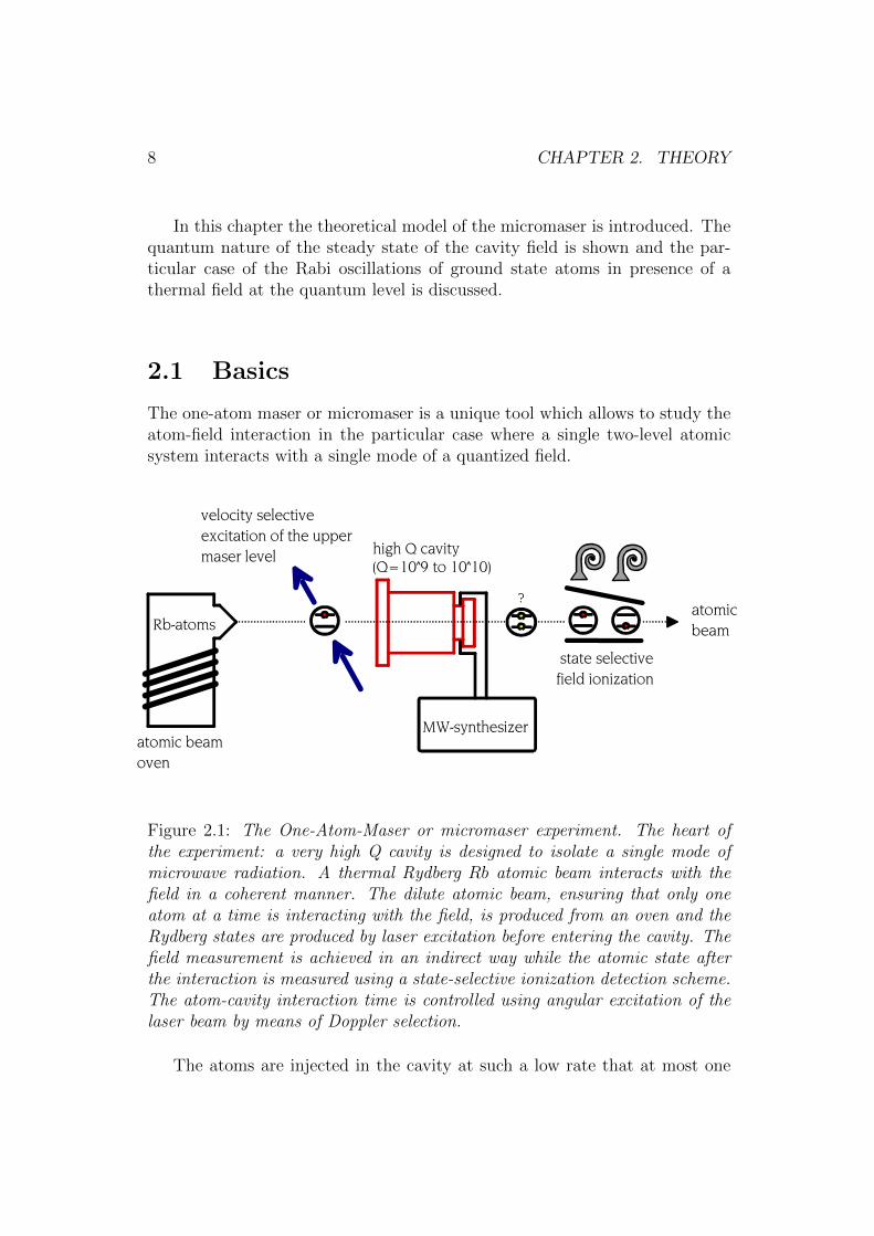
Figure 2.1: The One-Atom-Maser or micromaser experiment. The heart ofthe experiment: a very high Q cavity is designed to isolate a single mode ofmicrowave radiation. A thermal Rydberg Rb atomic beam interacts with thefield in a coherent manner. The dilute atomic beam, ensuring that only oneatom at a time is interacting with the field, is produced from an oven and theRydberg states are produced by laser excitation before entering the cavity. Thefield measurement is achieved in an indirect way while the atomic state afterthe interaction is measured using a state-selective ionization detection scheme.The atom-cavity interaction time is controlled using angular excitation of thelaser beam by means of Doppler selection.
The atoms are injected in the cavity at such a low rate that at most one
2.1. BASICS 9
atom at a time is present in the cavity. In the case of the micromaser we haveto deal with an open quantum system under further assumptions:
• Atom-field interaction involves only one mode of the field and a two-levelRydberg atom with the ground maser level |g〉 as the 61D 5
2state and
the excited maser level |e〉 the 63P 32
state of the 85Rb atom. Due to thecavity geometry only one mode is near resonant.
• The atom-field interaction time τ is controlled via Doppler selection ofthe velocity of the atoms in the excitation scheme.
• The coupling g of the atom to the field is much stronger than the cou-pling between the atom or the cavity to the environment (γ and κ ): themicromaser operates in the strong coupling regime.
• The atom-field interaction is a dipole-dipole coupling between a singlemode of a field and two well-known Rydberg states of the atoms.
In order to describe the dynamics of the mircomaser, the description of theelectromagnetic field of the cavity has to be outlined first. From the Maxwellsequations (in MKS unit) restricted to a charge-free (e.g. vacuum), isotropicand homogenous media:
∇.E = 0 (2.1)
∇.H = 0 (2.2)
∇×H− ε0 E = 0 (2.3)
∇× E + µ0 H = 0 (2.4)
Consider the electric field E(r,t) and magnetic field H inside a volume Vbounded by a surface S of perfect conductivity. E and H can be decomposedin terms of two sets of orthogonalized and normalized vector fields (modes) Ea
and Ha .These sets Ea and Ha obey to the Slater relations [25] :
kaEa = ∇×Ha (2.5)
kaHa = ∇× Ea (2.6)
10 CHAPTER 2. THEORY
From the wave equations (2.5) and (2.6), one recovers the Helmotz equationsfor Ea and Ha :
∇2 Ea + k2a Ea = 0 (2.7)
∇2 Ha + k2a Ha = 0 (2.8)
By using the separation of variables, the total resonator fields, E(r, t) andH(r, t), can then be decomposed as:
E(r, t) = −∑a
1√ε0pa(t) Ea(r) (2.9)
H(r, t) =∑a
1õ0
ωaqa(t) Ha(r) (2.10)
with ωa = ka/√µ0ε0. Using the Maxwell equations and the Slater relations
leads to the relations for pa and qa:
pa = qa
ω2aqa = −pa (2.11)
In order to find a model for the quantization of a field in a cavity, we startby writing down the total energy of the field inside the cavity. The Hamiltonianof the system is:
H =1
2
∫v
µ0 H.H + ε0 E. E dv (2.12)
Replacing E(r, t) and H(r, t) by their expressions obtain in (2.9) and (2.10)gives:
H =∑a
1
2(p2a + ω2
aq2a) (2.13)
From the relations between pa and qa (2.11) obtained from the Maxwell’ equa-tions we see that pa and qa constitute a canonically conjugate pair and aresolutions of the Hamiltons equations of motion relating qa to pa and pa to qa.
The quantization of the electromagnetic field is then achieved by consider-ing pa and qa as formally equivalent to the momentum and coordinate operatorof a quantum mechanical oscillator. They then obey to the commutator rela-tions:
[pa, pb] = [qa, qb] = 0
[pa, qb] = i~δa,b (2.14)
2.2. THE JAYNES-CUMMINGS MODEL 11
We introduce at this point the creation operator a†b and the annihilationoperator ab by:
a†b(t) =
(1
2~ωb
) 12
[ωb qb(t) − i pb(t)] (2.15)
ab(t) =
(1
2~ωb
) 12
[ωb qb(t) + i pb(t)] (2.16)
From (2.15) and (2.16) we find directly the commutator relations to be:
[aa, ab] = [a†a, a†b] = 0
[aa, a†b] = δa,b (2.17)
Replacing the operator p and q by the operator a and a† in (2.14), the Hamiltonoperator of a quantum field reads:
H =∑b
~ωb(a†bab +1
2) (2.18)
2.2 The Jaynes-Cummings model
To describe the interaction between the atoms and the cavity field, we have touse the well-known Jaynes-Cummings Hamiltonian[6]. It deals with the casewhen a single mode of a quantized electromagnetic field couples to a two-levelsystem.
In the case of the micromaser experiment, the two-level system is formedby the Rydberg atomic states where the ground maser level |g〉 is the 61D5/2
state and the excited maser level |e〉 the 63P3/2 state of the 85Rb atom.The Hamiltonian HA of the atomic system can so be written as,
HA =1
2~ωA(σ†σ − σσ†) (2.19)
The energy gap between the two levels is ωA. The transition between the twoatomic states is described by the operators σ = |g〉〈e| and σ† = |e〉〈g|. Theseoperators satisfy the fermionic anticommutation relation:
[σ, σ†]+ = σσ† + σ†σ = 1 (2.20)
and the commutator reads:
[σ, σ†] = |e〉〈e| − |g〉〈g| = σz (2.21)
12 CHAPTER 2. THEORY
This comes to a simple expression for the atom Hamiltonian:
HA =1
2~ωAσz (2.22)
In the same way one can rewrite the position operator ~r of the electronto the nuclei in the |e〉 ,|g〉 basis. Under the assumption that the atom hasno permanent dipole moment and that the matrix element are real, we have〈g|~r|e〉 = 〈e|~r|g〉 so,
~r = |g〉〈g|~r|e〉〈e|+ |e〉〈e|~r|g〉〈g|= (σ + σ†)〈e|~r|g〉 (2.23)
As the atomic transition is only resonant for one mode of the cavity field,the field Hamiltonian can be written as,
HF =1
2~ωF (a†a+
1
2) (2.24)
The quantum electric field along the atomic beam axis reads:
~E(~x) =E0√
2(a† + a) sin(k · z) (2.25)
where we assume that the field has a linear polarization along the x-axisand ~k ‖ ~z, with k = ωF
cand ωF the cavity frequency .
Assuming that the wavelength of the field is large compared to the dimen-sion of the Rydberg atoms, the interaction of the atom with the cavity fieldcan be described in a good approximation with the dipole approximation. Theinteraction Hamiltonian HAF can then be written as:
HAF = −e~r. ~E(~r) (2.26)
With (2.23) and (2.25), HAF reads:
HAF = ~g(σ† + σ)(a† + a) (2.27)
Where g [26] is the coupling constant:
g = −e〈g|x|e〉~
E0 sin(k · z) (2.28)
(2.27) has four different operators products which can be physically inter-preted:
• aσ corresponds to a photon absorption with the atomic transition |e〉 →|g〉, which corresponds to a loss of the total energy of the system.
2.2. THE JAYNES-CUMMINGS MODEL 13
• aσ† corresponds to the stimulated absorption.
• a†σ corresponds to the stimulated emission.
• a†σ† corresponds to a photon emission with the atomic transition |g〉 →|e〉, which corresponds to a gain of energy for the system.
Let us transform the atom-field Hamiltonian HAF in the Heisenberg represen-tation.
HAF = ~g(ae−iωF t + a†eiωF t)(σ†e−iωAt + σeiωAt) (2.29)
HAF = ~g(aσe−i(ωF +ωA)t + a†σ†ei(ωF +ωA)t + a†σei(ωF−ωA)t + aσ†e−i(ωA−ωF )t)(2.30)
If we integrate the Schrodinger equation in the Heisenberg representationwe get two oscillations terms:
1) a fast oscillation term ≈ 1ωF +ωA
2) a slow oscillation term ≈ 1ωF−ωA
As the slow term is dominant, we can neglected the fast one; this is calledthe rotating wave approximation. The expression of the atom-field Hamilto-nian is in this approximation:
HAF = ~g[aσ†e−i(ωF−ωA)t + a†σei(ωF−ωA)t] (2.31)
The neglected terms can lead to the Bloch-Zieget shift in the 2nd order of theperturbation theory [27].
HAF describes the Jaynes-Cummings interaction by finite detuning:
∆ = ωF − ωA
from the field respect to the atomic transition.The complete Hamiltonian of the system can then be written as:
HJC = HAF
= ~g(aσ†e−i∆t + a†σei∆t) (2.32)
14 CHAPTER 2. THEORY
This is the Jaynes-Cummings Hamiltonian. The new quantum state of thesystem is the tensor product between the field state and the atom state.
|i, n〉 = |i〉 ⊗ |n〉,where |i〉 ∈ |g〉, |e〉 (2.33)
The Jaynes-Cummings model can then be briefly summarized as follows:
• It is a fully quantum model describing the interaction between a two-level atomic system and the single mode of a quantized electromagneticfield by the means of the Hamiltonian (2.32).
• It is based on two approximations, namely the dipole approximation andthe rotating-wave approximation.
Having now this Hamiltonian at our disposal we can start to look closer tothe evolution of an atom-field system. Starting with an initial state where theatom is in his ground state |g〉 and the cavity in a number state |n+ 1〉:
Ψ(0) = |g, n+ 1〉 (2.34)
After a time τ , the wave function is:
Ψ(τ) = Cg,n+1(τ)|g, n+ 1〉+ Ce,n(τ)|e, n〉 (2.35)
with the Schrodinger equation thus,
Ψ(τ) = Ce,n(τ)|e, n〉+ Cg,n+1(τ)|g, n+ 1〉= −ig(aσ†e−i∆τ + a†σei∆τ )(Ce,n(τ)|e, n〉+ Cg,n+1(τ)|g, n+ 1〉) (2.36)
if we projet on |g, n〉 and |e, n− 1〉 we get:
Ce,n(τ) = −ig√n+ 1e−i∆τCg,n+1(τ) (2.37)
and,Cg,n+1(τ) = −ig
√n+ 1ei∆τCe,n(τ) (2.38)
If there is no detuning (∆ = 0) of the cavity to the atomic transition, with theinitial condition, we get:
Cg,n+1(τ) = cos(g√n+ 1τ) (2.39)
andCe,n(τ) = −i sin(g
√n+ 1τ) (2.40)
2.2. THE JAYNES-CUMMINGS MODEL 15
We can write so the probabilities P|g,n〉 and P|e,n−1〉 to observe the states|e, n〉 and |g, n+ 1〉,
P|g,n+1〉(τ) = |〈g, n+ 1||Ψ〉|2
= cos2(g√n+ 1τ) (2.41)
and,
P|e,n〉(τ) = |〈e, n||Ψ〉|2
= sin2(g√n+ 1τ) (2.42)
This describes the reversible emission of the atoms, this behavior is thequantum mechanical version of the Rabi oscillations where a two-level atomcoupled to a single mode electromagnetic field cavity alternately absorbs pho-ton(s) from the cavity mode and reemits them.
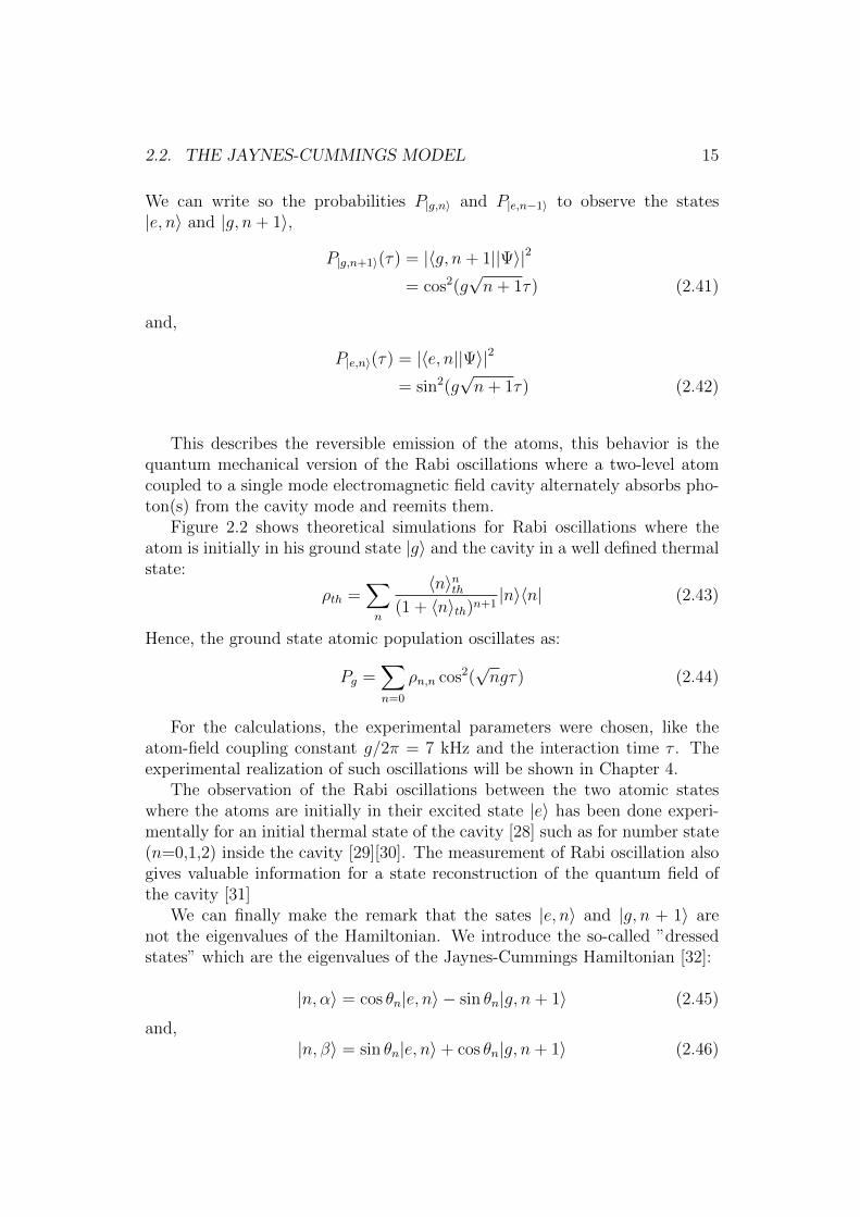
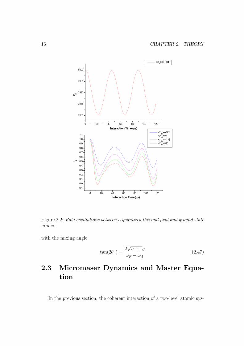
Figure 2.2 shows theoretical simulations for Rabi oscillations where theatom is initially in his ground state |g〉 and the cavity in a well defined thermalstate:
ρth =∑n
〈n〉nth(1 + 〈n〉th)n+1
|n〉〈n| (2.43)
Hence, the ground state atomic population oscillates as:
Pg =∑n=0
ρn,n cos2(√ngτ) (2.44)
For the calculations, the experimental parameters were chosen, like theatom-field coupling constant g/2π = 7 kHz and the interaction time τ . Theexperimental realization of such oscillations will be shown in Chapter 4.
The observation of the Rabi oscillations between the two atomic stateswhere the atoms are initially in their excited state |e〉 has been done experi-mentally for an initial thermal state of the cavity [28] such as for number state(n=0,1,2) inside the cavity [29][30]. The measurement of Rabi oscillation alsogives valuable information for a state reconstruction of the quantum field ofthe cavity [31]
We can finally make the remark that the sates |e, n〉 and |g, n + 1〉 arenot the eigenvalues of the Hamiltonian. We introduce the so-called ”dressedstates” which are the eigenvalues of the Jaynes-Cummings Hamiltonian [32]:
|n, α〉 = cos θn|e, n〉 − sin θn|g, n+ 1〉 (2.45)
and,|n, β〉 = sin θn|e, n〉+ cos θn|g, n+ 1〉 (2.46)
16 CHAPTER 2. THEORY
Figure 2.2: Rabi oscillations between a quantized thermal field and ground stateatoms.
with the mixing angle
tan(2θn) =2√n+ 1g
ωF − ωA(2.47)
2.3 Micromaser Dynamics and Master Equa-
tion
In the previous section, the coherent interaction of a two-level atomic sys-
2.3. MICROMASER DYNAMICS AND MASTER EQUATION 17
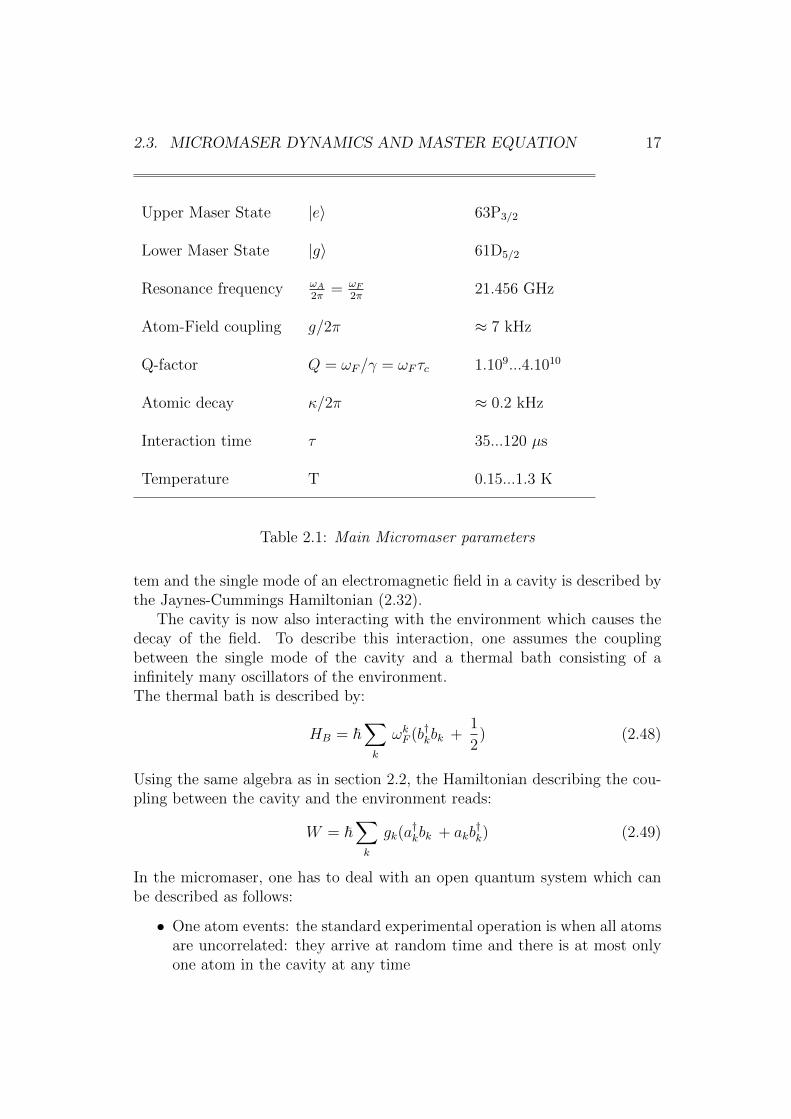
Upper Maser State |e〉 63P3/2
Lower Maser State |g〉 61D5/2
Resonance frequency ωA
2π= ωF
2π21.456 GHz
Atom-Field coupling g/2π ≈ 7 kHz
Q-factor Q = ωF/γ = ωF τc 1.109...4.1010
Atomic decay κ/2π ≈ 0.2 kHz
Interaction time τ 35...120 µs
Temperature T 0.15...1.3 K
Table 2.1: Main Micromaser parameters
tem and the single mode of an electromagnetic field in a cavity is described bythe Jaynes-Cummings Hamiltonian (2.32).
The cavity is now also interacting with the environment which causes thedecay of the field. To describe this interaction, one assumes the couplingbetween the single mode of the cavity and a thermal bath consisting of ainfinitely many oscillators of the environment.The thermal bath is described by:
HB = ~∑k
ωkF (b†kbk +1
2) (2.48)
Using the same algebra as in section 2.2, the Hamiltonian describing the cou-pling between the cavity and the environment reads:
W = ~∑k
gk(a†kbk + akb
†k) (2.49)
In the micromaser, one has to deal with an open quantum system which canbe described as follows:
• One atom events: the standard experimental operation is when all atomsare uncorrelated: they arrive at random time and there is at most onlyone atom in the cavity at any time
18 CHAPTER 2. THEORY
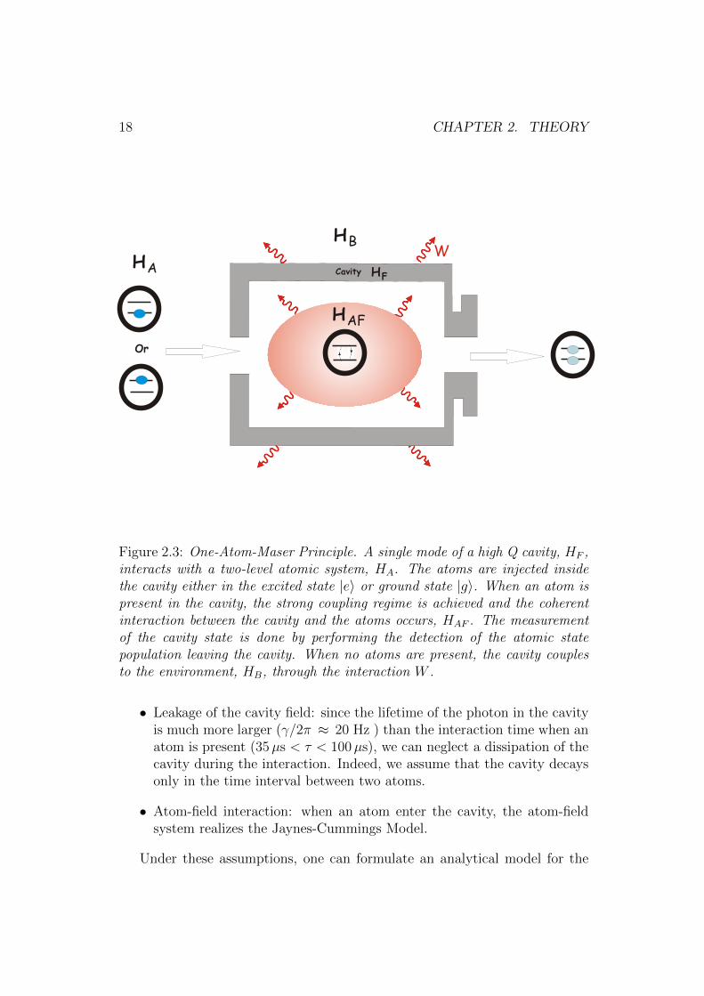
Cavity
HB
HAF
HF
W
Or
HA
Figure 2.3: One-Atom-Maser Principle. A single mode of a high Q cavity, HF ,interacts with a two-level atomic system, HA. The atoms are injected insidethe cavity either in the excited state |e〉 or ground state |g〉. When an atom ispresent in the cavity, the strong coupling regime is achieved and the coherentinteraction between the cavity and the atoms occurs, HAF . The measurementof the cavity state is done by performing the detection of the atomic statepopulation leaving the cavity. When no atoms are present, the cavity couplesto the environment, HB, through the interaction W .
• Leakage of the cavity field: since the lifetime of the photon in the cavityis much more larger (γ/2π ≈ 20 Hz ) than the interaction time when anatom is present (35µs < τ < 100µs), we can neglect a dissipation of thecavity during the interaction. Indeed, we assume that the cavity decaysonly in the time interval between two atoms.
• Atom-field interaction: when an atom enter the cavity, the atom-fieldsystem realizes the Jaynes-Cummings Model.
Under these assumptions, one can formulate an analytical model for the

2.3. MICROMASER DYNAMICS AND MASTER EQUATION 19
micromaser [14, 33]. Considering the micromaser dynamics as two separableterms, namely a pumping process of the cavity field in presence of the atomsand a relaxation process when no atoms are present the time evolution of thefield reads:
∂ρ
∂t=
(∂ρ
∂t
)gain
+
(∂ρ
∂t
)loss
(2.50)
The decay of the cavity is modeled by the interaction W (2.49) couplingthe single mode of the cavity to an external thermal bath. This model hasa standard description and its evolution is given by the mean of the masterequation of a damped harmonic oscillator [34] :(
∂ρ
∂t
)loss
= Lρ
= −1
2γ(nth + 1)(a†aρ− 2aρa† + ρa†a) (2.51)
− 1
2γnth(a
†aρ− 2aρa† + ρa†a)
where nth = (e~ω
kBT )−1 is the mean thermal photon number. Here the evolutionoperator L is called the Liouvillian operator.
The pump process is assimilated to the atom field interaction. Startingfrom the Jaynes-Cummings Hamiltonian (2.32) the unitary evolution operatorU(τ) reads:
U(τ) = e−(i/~)HJCτ
= cos(gτ√a†a+ 1
)|e〉〈e|+ cos
(gτ√a†a+ 1
)|g〉〈g|
− isin(gτ√a†a+ 1
)√a†a+ 1
a|e〉〈g| − isin(gτ√a†a)
√a†a
a†|g〉〈e| (2.52)
The change of the cavity per atom is given by:
δρ = ρ(to + τ)− ρ(t0) (2.53)
where ρ(t0 + τ) can be expressed as:
ρ(t0 + τ) = TraU †(τ)ρa+f (t0)U(τ)= Aρ+ Bρ (2.54)
with,
Aρ = Pe(t0) cos(gτ√a†a+ 1
)ρ(t0) cos
(gτ√a†a+ 1
)+
Pe(t0)a†sin(gτ√a†a+ 1
)√a†a+ 1
ρ(to)sin(gτ√a†a+ 1
)√a†a+ 1
a (2.55)

20 CHAPTER 2. THEORY
Bρ = Pg(t0) cos(gτ√a†a)ρ(t0) cos
(gτ√a†a)
+
Pg(t0)asin(gτ√a†a)
√a†a
ρ(to)sin(gτ√a†a)
√a†a
a† (2.56)
0
0,05882
0,1176
0,1765
0,2353
0,2941
0,3529
0,4118
0,4706
0,5294
0,5882
0,6471
0,7059
0,7647
0,8235
0,8824
0,9412
1,000
0 20 40 60 80 100 120 140
interaction time [m s]
mean photon
number
0
2
4
6
8
10
12
14
photon number
color co
ded probability
Figure 2.4: One-Atom-Maser Pumpcurve: the red line represents the meanphoton number of the cavity. Around the mean photon number, photon fieldstates with sub-Poissonian statistic are present. In particularly, bistability canbe observed for an interaction time τ = 57µs. The marked depth show thepresence of trapping state, Fock states, produced in the cavity
In order to get only the time evolution of the cavity field, we have tracedover the atomic state and Pe(t0) and Pg(t0) are the probabilities that the atomenters either in the excited or ground state. Hence the overall change of thecavity field due to the interaction with the atomic beam reads:
∆ρ = R∆t(ρ(t0 + τ)− ρ(t0)) (2.57)
2.3. MICROMASER DYNAMICS AND MASTER EQUATION 21
The gain term in the master equation can then be written as follows:(∂ρ
∂t
)gain
= R(A+ B − 1)ρ (2.58)
where R is the atomic beam rate - number of atoms per cavity decay time.Substituting (2.49) and (2.56) in the master equation (2.48) leads to the generalmicromaser master equation:
∂ρ
∂t= R(A+ B − 1 + L)ρ (2.59)
This equation describes an open driven quantum system and can be solvedin the steady-state regime when the gains are equal to the losses, ∂ρ
∂t= 0 . The
resulting equation leads to the following recursion:
ρnn =nthγ + Ek
(nth + 1)γ + Gkρn−1 (2.60)
The steady-state solution ρssnn reads:
ρssnn = ρss00
n∏k=1
nthγ + Ek(nth + 1)γ + Gk
(2.61)
with the coefficients:
Ek =Re
ksin2(√kgτ) (2.62)
Gk =Rg
ksin2(√kgτ) (2.63)
and Ri is the rate at which the atoms are injected into the state |i〉(= |e〉 or|g〉) per cavity decay time.
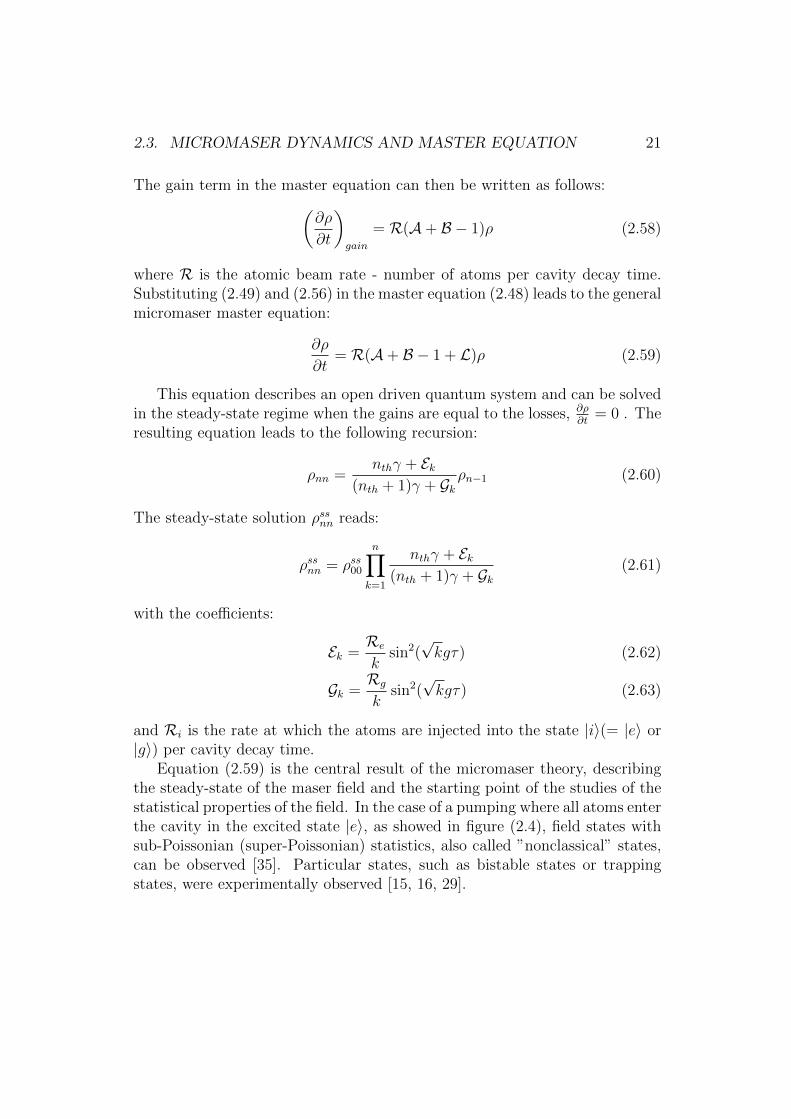
Equation (2.59) is the central result of the micromaser theory, describingthe steady-state of the maser field and the starting point of the studies of thestatistical properties of the field. In the case of a pumping where all atoms enterthe cavity in the excited state |e〉, as showed in figure (2.4), field states withsub-Poissonian (super-Poissonian) statistics, also called ”nonclassical” states,can be observed [35]. Particular states, such as bistable states or trappingstates, were experimentally observed [15, 16, 29].

22 CHAPTER 2. THEORY
Chapter 3
Experimental Setup
In this chapter, the experimental setup of the micromaser is developed. Thegeneration of a controlled atomic beam and the high Q superconuctive cavity areintroduced. The most relevant properties of the 85Rb Rydberg atoms are stud-ied. In particular the coupling constant is reevaluated and the Rydberg lifetimeof the maser ground state, 61D5/2 is recalculated using the latest theoreticalcontribution. Improvements of the cryogenic system, leading to a continuallycontrolable cooling temperature from 1.3 K down to 150 mK, are explained.
The experimental realization of the theoretical Jaynes-Cummings modelwhere a single two-level atom couples to a single mode of the field of a cavityis achieved with the micromaser experiment. The experimental idea of themicromaser is based on the MASER realized by Townes and co-workers [36],where an ammoniac molecular beam interacts with a low Q microwave cavity.In order to achieve the strong coupling regime where the dynamics is dominatedby the coherent interaction between a two-level system and a single modeof radiation, highly excited Rydberg atoms and a high Q superconductingniobium cavity are used.
Cavities offering the longest lifetime are obtained in the microwave domainat frequencies of several tens of gigahertz (GHz) for wavelength λ of the order ofthe centimeter. Since the microwave photon energy is smaller than the energygap of certain superconductive materials, the photon absorption at the surfaceis reduced. The resistivity of a superconductor vanishing at absolute zero[37]. Long storage time of the microwave field on the order of few hundredmillisecond in the cavity can be achieved. The superconducting Nb cavityused in the micromaser experiment has a cylindrical form and has two smallcoupling holes along the atomic beam axis. The cavity is also designed to fulfillthe experiments requirements:
• Only one mode of the cavity is resonant with the atomic transition .
23

24 CHAPTER 3. EXPERIMENTAL SETUP
• The decay rate of the cavity field for this mode has to be small enoughto achieve the strong coupling condition: γ << g (see Chapter 2).
The microwave transitions traditionally used in atomic physics (Zeemantransitions or hyperfine transitions) are not adapted to the realization of thestrong coupling regime due to their very small coupling to an electromagneticfield. Hence, highly excited atoms, Rydberg atoms, are used. Rydberg atomspresent many advantages:
• Rydberg-Rydberg atomic transitions, which are in the microwave region,present a large dipole moment as the wave functions of two neighboringstates strongly overlap.
• Long lifetime with respect to the ground state as the wave function isstrongly delocalized from the nucleus.
• Easily produced by laser field excitation.
• State-selective detection in DC-electric fields.
Figure 3.1 shows an overview of the experimental setup. The experiment is ina vacuum environment. This is done by means of turbo-molecular pump anda vacuum of the order of 5.10−7 mbar is achieved. For the realization of themicromaser experiment:
• A very dilute and stable Rb atomic beam is produced from an oven.
• 85Rb atoms are prepared in the maser state |g〉 = 61D5/2 atomic stateand |e〉 = 63P3/2 atomic state by the mean of different laser excitation.
• A cryogenic environment is needed to work with a low thermal photonnumber and operate the superconducting Nb cavity as high Q cavity inorder to achieve the strong coupling regime.
25
Turbo Molecular Vacuum Pumps
Rb Oven
Cryostat
CavityField IonizationDetection SystemAtomic Beam
Liquid N tankAuxiliaryDetectionSystem
Heat Shield
X-Y Translation Stage
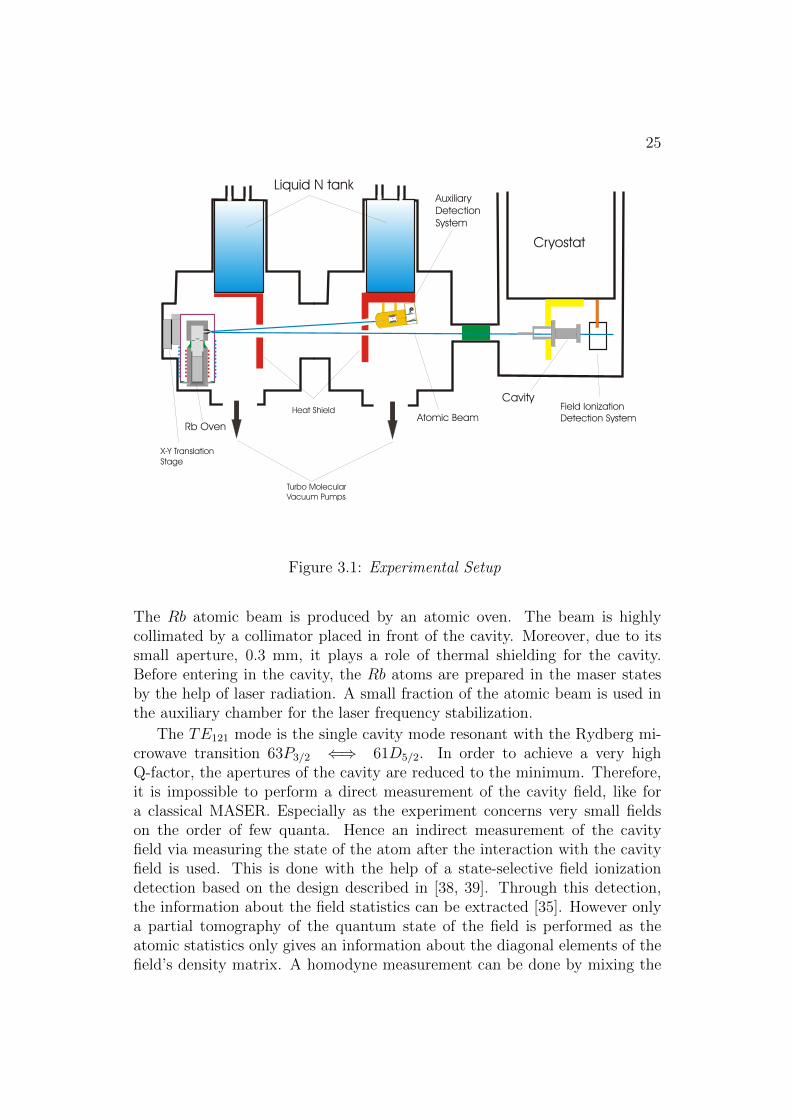
Figure 3.1: Experimental Setup
The Rb atomic beam is produced by an atomic oven. The beam is highlycollimated by a collimator placed in front of the cavity. Moreover, due to itssmall aperture, 0.3 mm, it plays a role of thermal shielding for the cavity.Before entering in the cavity, the Rb atoms are prepared in the maser statesby the help of laser radiation. A small fraction of the atomic beam is used inthe auxiliary chamber for the laser frequency stabilization.
The TE121 mode is the single cavity mode resonant with the Rydberg mi-crowave transition 63P3/2 ⇐⇒ 61D5/2. In order to achieve a very highQ-factor, the apertures of the cavity are reduced to the minimum. Therefore,it is impossible to perform a direct measurement of the cavity field, like fora classical MASER. Especially as the experiment concerns very small fieldson the order of few quanta. Hence an indirect measurement of the cavityfield via measuring the state of the atom after the interaction with the cavityfield is used. This is done with the help of a state-selective field ionizationdetection based on the design described in [38, 39]. Through this detection,the information about the field statistics can be extracted [35]. However onlya partial tomography of the quantum state of the field is performed as theatomic statistics only gives an information about the diagonal elements of thefield’s density matrix. A homodyne measurement can be done by mixing the
26 CHAPTER 3. EXPERIMENTAL SETUP
quantum field of the one atom maser with an external coherent field and mapthe phase information into the atomic statistics [40].
In the following sections, the description of the atomic beam productionwill be explained. An introduction to Rydberg atoms and their more relevantproperties for the micromaser experiments will be discussed. Finally in thetwo last sections, the high Q-factor cavity will be described and the cryogenicsystem will be explained.
3.1 Atomic Beam
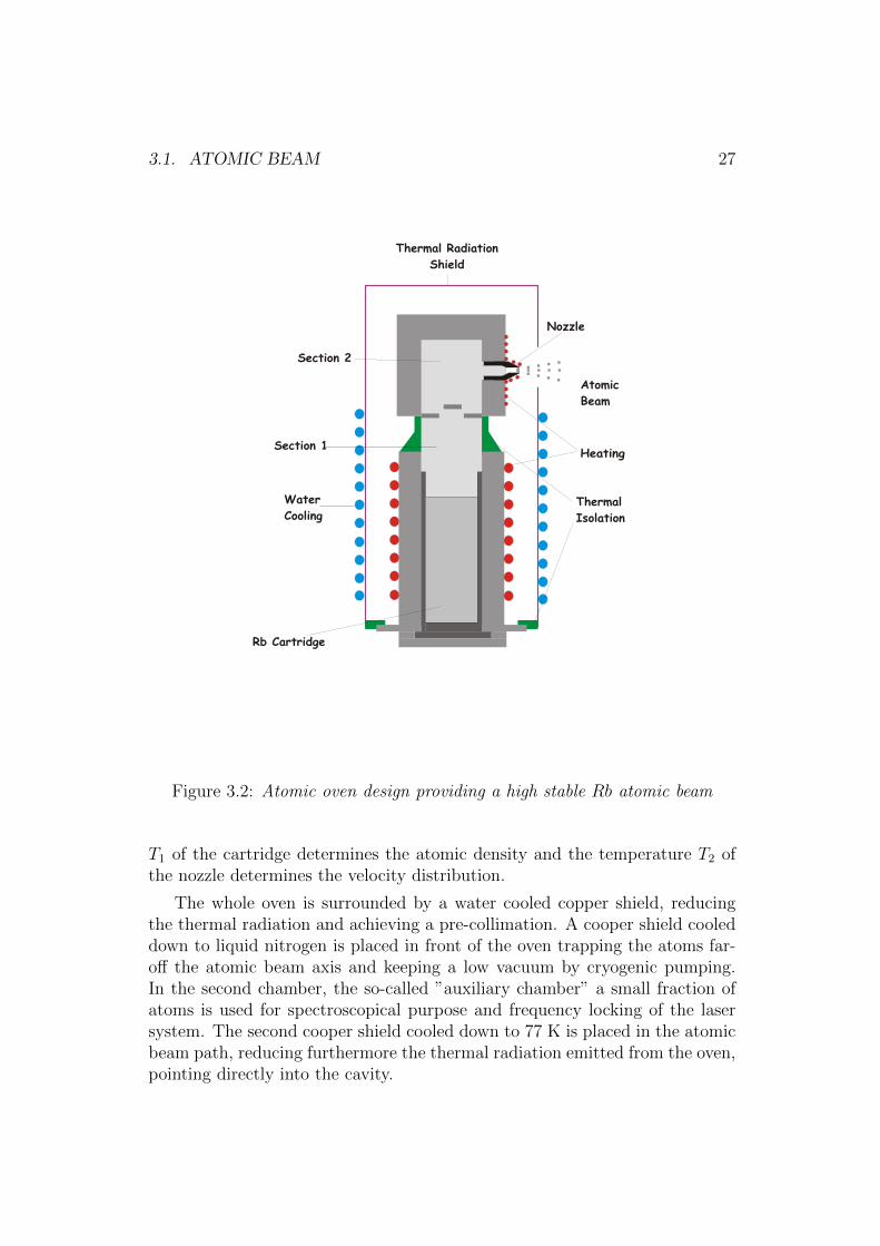
A scheme of the atomic oven is shown in figure 3.2. It consists of two stainlesssteel cylinders separated by an insulating material providing a thermal isolationbetween the two parts. The lower cylinder consists of a cartridge of rubidiumand is mounted from below. The cartridge can be individually heated up witha resistance wire well above the Rb melting point at around 470K creatinga Rb buffer gas in the upper part. The independent control over the heatingtemperature T1 in the section 1 allows to determine how muchRb is evaporated,controlling the gas pressure in the oven and finally allows an independentadjustment of the atomic density flux.
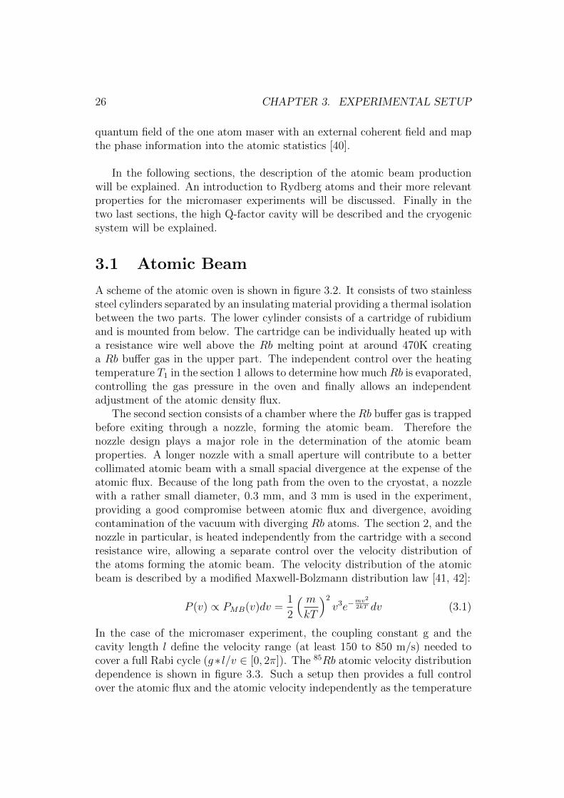
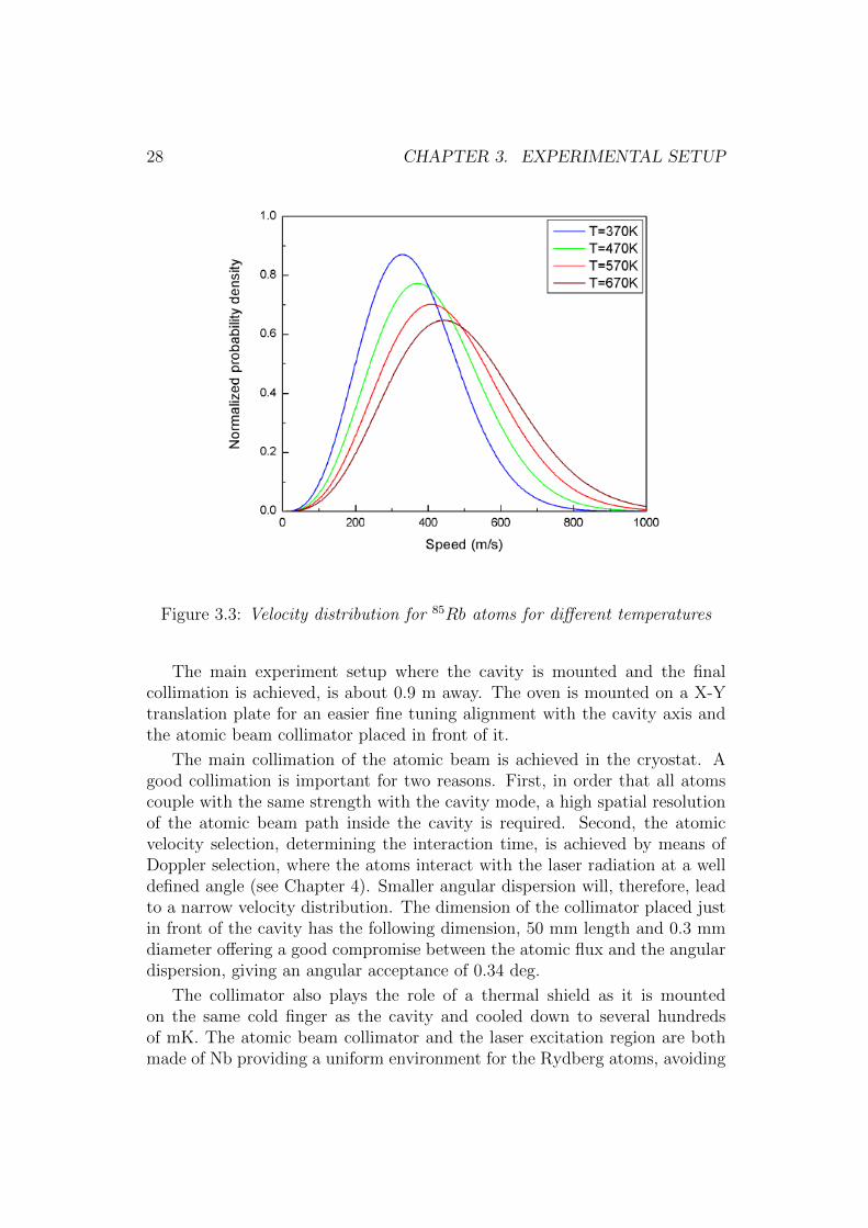
The second section consists of a chamber where the Rb buffer gas is trappedbefore exiting through a nozzle, forming the atomic beam. Therefore thenozzle design plays a major role in the determination of the atomic beamproperties. A longer nozzle with a small aperture will contribute to a bettercollimated atomic beam with a small spacial divergence at the expense of theatomic flux. Because of the long path from the oven to the cryostat, a nozzlewith a rather small diameter, 0.3 mm, and 3 mm is used in the experiment,providing a good compromise between atomic flux and divergence, avoidingcontamination of the vacuum with diverging Rb atoms. The section 2, and thenozzle in particular, is heated independently from the cartridge with a secondresistance wire, allowing a separate control over the velocity distribution ofthe atoms forming the atomic beam. The velocity distribution of the atomicbeam is described by a modified Maxwell-Bolzmann distribution law [41, 42]:
P (v) ∝ PMB(v)dv =1
2
( mkT
)2
v3e−mv2
2kT dv (3.1)
In the case of the micromaser experiment, the coupling constant g and thecavity length l define the velocity range (at least 150 to 850 m/s) needed tocover a full Rabi cycle (g∗ l/v ∈ [0, 2π]). The 85Rb atomic velocity distributiondependence is shown in figure 3.3. Such a setup then provides a full controlover the atomic flux and the atomic velocity independently as the temperature
3.1. ATOMIC BEAM 27
Heating
Nozzle
Section 1
Section 2
Thermal Radiation
Shield
Thermal
Isolation
Water
Cooling
Rb Cartridge
Atomic
Beam
Figure 3.2: Atomic oven design providing a high stable Rb atomic beam
T1 of the cartridge determines the atomic density and the temperature T2 ofthe nozzle determines the velocity distribution.
The whole oven is surrounded by a water cooled copper shield, reducingthe thermal radiation and achieving a pre-collimation. A cooper shield cooleddown to liquid nitrogen is placed in front of the oven trapping the atoms far-off the atomic beam axis and keeping a low vacuum by cryogenic pumping.In the second chamber, the so-called ”auxiliary chamber” a small fraction ofatoms is used for spectroscopical purpose and frequency locking of the lasersystem. The second cooper shield cooled down to 77 K is placed in the atomicbeam path, reducing furthermore the thermal radiation emitted from the oven,pointing directly into the cavity.
28 CHAPTER 3. EXPERIMENTAL SETUP
Figure 3.3: Velocity distribution for 85Rb atoms for different temperatures
The main experiment setup where the cavity is mounted and the finalcollimation is achieved, is about 0.9 m away. The oven is mounted on a X-Ytranslation plate for an easier fine tuning alignment with the cavity axis andthe atomic beam collimator placed in front of it.
The main collimation of the atomic beam is achieved in the cryostat. Agood collimation is important for two reasons. First, in order that all atomscouple with the same strength with the cavity mode, a high spatial resolutionof the atomic beam path inside the cavity is required. Second, the atomicvelocity selection, determining the interaction time, is achieved by means ofDoppler selection, where the atoms interact with the laser radiation at a welldefined angle (see Chapter 4). Smaller angular dispersion will, therefore, leadto a narrow velocity distribution. The dimension of the collimator placed justin front of the cavity has the following dimension, 50 mm length and 0.3 mmdiameter offering a good compromise between the atomic flux and the angulardispersion, giving an angular acceptance of 0.34 deg.
The collimator also plays the role of a thermal shield as it is mountedon the same cold finger as the cavity and cooled down to several hundredsof mK. The atomic beam collimator and the laser excitation region are bothmade of Nb providing a uniform environment for the Rydberg atoms, avoiding
3.2. RYDBERG ATOMS 29
contact potential with the resonator, with a stable zero magnetic field and ata constant temperature.
3.2 Rydberg Atoms
Rydberg atoms are excited atomic systems where an electron has been pro-moted to a level with large principal quantum number n. Their radiativeproperties are very interesting for several reasons: first, the large electric dipolematrix elements between neighboring levels - proportional to n2- are typicallythree orders of magnitude larger than for atomic system in the ground state orlower excited state. Then, the coupling to a radiation field is very strong. Sec-ond, these atoms have very long spontaneous emission lifetimes, which meansthat one can manipulate them for a long time without loss of the atomic co-herences.
The first experiment on Rydberg atoms was done by the end of the 19th
century as Balmer measured in 1885 the hydrogen line and derived the Balmer-formula. In 1890 Rydberg started to classify, by series, the spectral ray ofAlkali-atom in the form of S=sharp, P=principal, D=diffuse[43] leading tothe relation in energy:
νl = ν∞l −RRyd
(n− δl)2for l = S, P,D (3.2)
where ν∞l is the limit of the series, RRyd = 109721.6 cm−1 the Rydberg con-stant and δl the quantum defect. From these relations one can derive theenergy difference between two energy states and then define the transition fre-quency between these two states. The meaning of n became then clear withthe introduction of Bohr’s Hydrogen Model, as the principal quantum numberdescribing the orbit of the electron around the nucleus. The electron bidingenergy W to the nucleus can be then written for the hydrogen atom as:
W = − e4me
32π2ε0~1
n2= −RRyd
n2(3.3)
As the atom size also grows with n2, the large size of the Rydberg atomscombined with the small transition probabilities lead to a very long lifetimeof the Rydberg states. Lifetimes up to 50 ms were measured [44]. There aremany different ways to produce Rydberg atoms. The most probable is therecombination of ions. This occurs when ions collide with neutral particlesand exchange charges or by recombination of ions with electrons [45]. Therecombination process plays a major role in plasma physics. The disadvantageof these methods are that the final Rydberg states can not be determined.
30 CHAPTER 3. EXPERIMENTAL SETUP
Rydberg atoms can also be produced by means of laser radiation, which isthe technique used for this work. The use of a narrow laser transition allow topopulate only the target Rydberg states. Moreover coherent population canbe achieved [46].
In this work 85Rb atoms are used. They are alkali atoms and hydrogen-like as only one electron is sitting in the outer shell. The difference betweenhydrogen and hydrogen-like atoms is that the electron does not see only aproton but a nucleus with an electron cloud forming a positive charge entity.In this system, the energy levels of the outer electron are shifted compare tothe hydrogen atom. The energy shift can be calculated as we exchange themain quantum number n by the effective quantum number n∗ :
n∗ = n− δn,j,l (3.4)
where δn,j,l is called the quantum defect [47]. The quantum defect can becalculated by the Rydberg-Ritz formula:
δn,j,l = δ0 +δ2
(n− δ0)2+
δ4
(n− δ0)4+
δ6
(n− δ0)6+
δ8
(n− δ0)8.... (3.5)
The δi coefficient are experimentally determined and were lately improved forRb atoms with absolute frequency measurements in an atomic beam [48]. Theenergy level of the Rydberg states can then be recalculated:
W = −R′
Ryd
(n∗)2= −
R′
Ryd
(n− δn,j,l)2(3.6)
with R′Ryd is the particular element Rydberg constant. In the case of 85Rb, itvalues 109736.605 cm−1 [49].
In the following sub-section, the main properties of the Rydberg states usedfor the micromaser will be briefly described.
Microwave Transitions between Rydberg Levels
The transition frequency between two neighboring Rydberg states scaleswith the main quantum number n−3:
ωnl→n′l′ ∼2RRyd
n3(3.7)
For Rydberg transitions with n ≈ 50 . . . 65, the transitions are in the microwaveregime of the order of tens of GHz. In the micromaser, the Rydberg transition63P3/2 ⇐⇒ 61D5/2 in 85Rb at 21.456 GHz is used.
3.2. RYDBERG ATOMS 31
The matrix element µ for the dipole interaction between two Rydberg statesscales proportional to n2:
µ = 〈nl|er|n′l′〉 ∼ e ao n2 (3.8)
Typical values for µ with n = 60 are three orders of magnitude larger than foroptical transitions and are much larger than microwave hyperfine or Zeemantransitions used traditionally in atomic physics. The exact value of the dipolematrix element can be determined with the help of a model presented in [50,51, 52, 53]. For the maser Rydberg transition 63P3/2 ⇐⇒ 61D5/2:
µ
ea0
∼ 1355 (3.9)
The vacuum Rabi frequency Ω for the coupling of the two Rydberg level atomsystem with the single mode of a cavity can then be calculated using therelation:
~Ω = µE0 (3.10)
with E0 given by (2.25). In the case of the micromaser experiment, the vacuumRabi frequency is ∼ 7.2 kHz.
Rydberg Atoms Lifetime
One of the most important properties of the Rydberg atoms for their ap-plication in the maser are their long lifetime. Namely, in order to realize acoherent interaction, the Rydberg atomic states have to survive during thewhole experiment. This implies, that there is no decay into the atomic groundstate during the interaction with the cavity mode. Also, as no direct mea-surement of the field can be achieved, the measurement of the atomic stateprovides an indirect measurement of the cavity field. Therefore, a decay ofthe atomic state would lead to a loss of information. The time of flight of theRydberg atoms from their production till their detection, is typically on theorder of few 100µs.
The lifetime of highly excited states can be very large. If only one decaychannel to a lower state exists, the lifetime τ of the excited state is then givenby the inverse of the Einstein An′,l′,n,l coefficient. In the case of Rydbergstates, more than one decay channel is available, and τ can be then calculatedby summing over all possibilities:
1
τ=∑n,l
An′,l′,n.l (3.11)
32 CHAPTER 3. EXPERIMENTAL SETUP
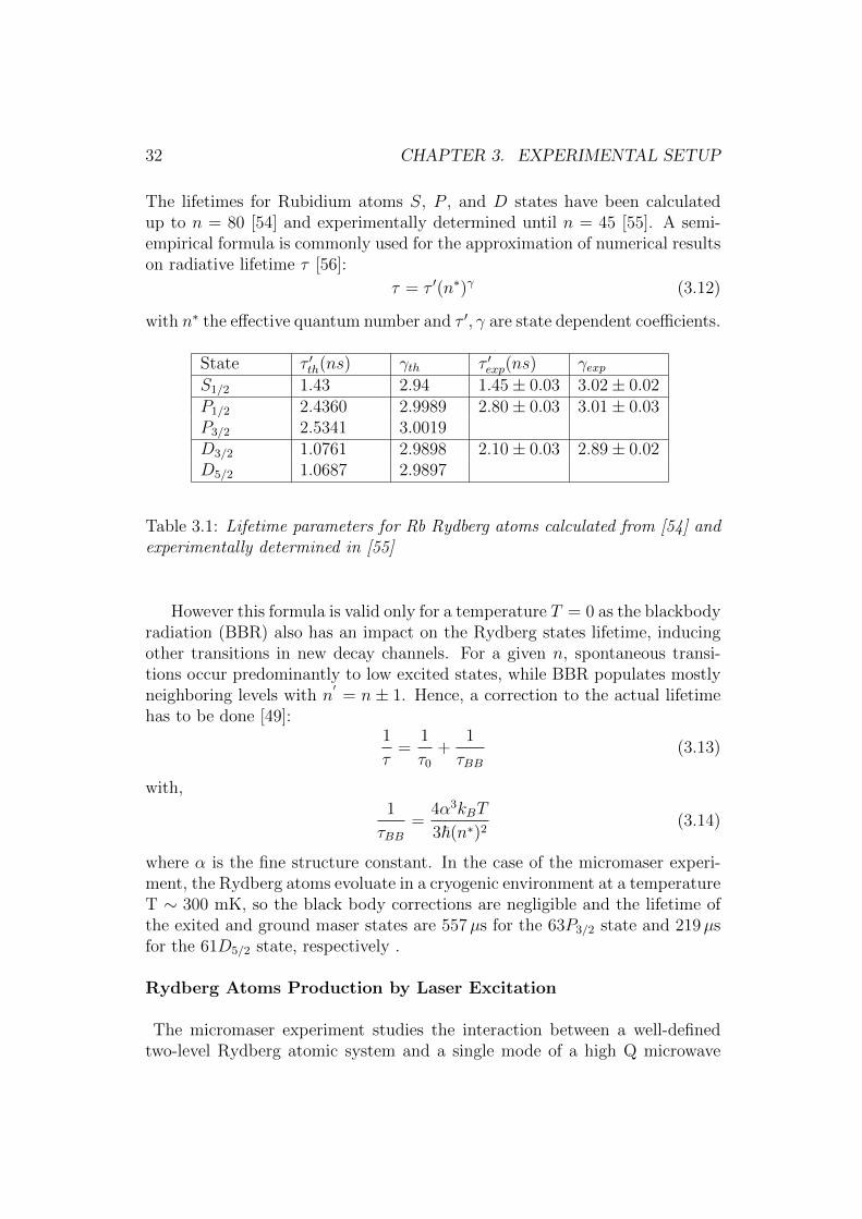
The lifetimes for Rubidium atoms S, P , and D states have been calculatedup to n = 80 [54] and experimentally determined until n = 45 [55]. A semi-empirical formula is commonly used for the approximation of numerical resultson radiative lifetime τ [56]:
τ = τ ′(n∗)γ (3.12)
with n∗ the effective quantum number and τ ′, γ are state dependent coefficients.
State τ ′th(ns) γth τ ′exp(ns) γexpS1/2 1.43 2.94 1.45± 0.03 3.02± 0.02P1/2 2.4360 2.9989 2.80± 0.03 3.01± 0.03P3/2 2.5341 3.0019D3/2 1.0761 2.9898 2.10± 0.03 2.89± 0.02D5/2 1.0687 2.9897
Table 3.1: Lifetime parameters for Rb Rydberg atoms calculated from [54] andexperimentally determined in [55]
However this formula is valid only for a temperature T = 0 as the blackbodyradiation (BBR) also has an impact on the Rydberg states lifetime, inducingother transitions in new decay channels. For a given n, spontaneous transi-tions occur predominantly to low excited states, while BBR populates mostlyneighboring levels with n
′= n± 1. Hence, a correction to the actual lifetime
has to be done [49]:1
τ=
1
τ0
+1
τBB(3.13)
with,1
τBB=
4α3kBT
3~(n∗)2(3.14)
where α is the fine structure constant. In the case of the micromaser experi-ment, the Rydberg atoms evoluate in a cryogenic environment at a temperatureT ∼ 300 mK, so the black body corrections are negligible and the lifetime ofthe exited and ground maser states are 557µs for the 63P3/2 state and 219µsfor the 61D5/2 state, respectively .
Rydberg Atoms Production by Laser Excitation
The micromaser experiment studies the interaction between a well-definedtwo-level Rydberg atomic system and a single mode of a high Q microwave
3.2. RYDBERG ATOMS 33
780 nm
297 nm
w/2p = 21.456 GHZ
480 nm
Rb85
63P3/2
61D 5/2
5P3/2
5S1/2
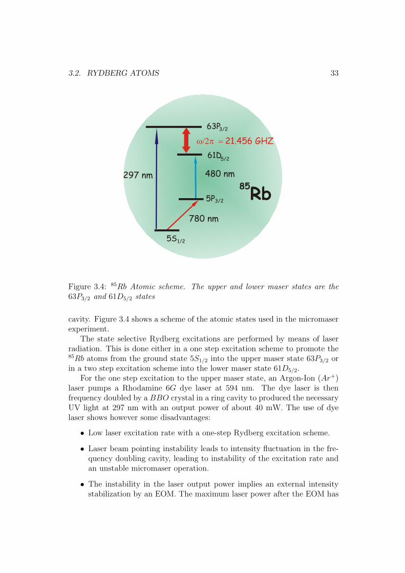
Figure 3.4: 85Rb Atomic scheme. The upper and lower maser states are the63P3/2 and 61D5/2 states
cavity. Figure 3.4 shows a scheme of the atomic states used in the micromaserexperiment.
The state selective Rydberg excitations are performed by means of laserradiation. This is done either in a one step excitation scheme to promote the85Rb atoms from the ground state 5S1/2 into the upper maser state 63P3/2 orin a two step excitation scheme into the lower maser state 61D5/2.
For the one step excitation to the upper maser state, an Argon-Ion (Ar+)laser pumps a Rhodamine 6G dye laser at 594 nm. The dye laser is thenfrequency doubled by a BBO crystal in a ring cavity to produced the necessaryUV light at 297 nm with an output power of about 40 mW. The use of dyelaser shows however some disadvantages:
• Low laser excitation rate with a one-step Rydberg excitation scheme.
• Laser beam pointing instability leads to intensity fluctuation in the fre-quency doubling cavity, leading to instability of the excitation rate andan unstable micromaser operation.
• The instability in the laser output power implies an external intensitystabilization by an EOM. The maximum laser power after the EOM has

34 CHAPTER 3. EXPERIMENTAL SETUP
to be on the order of one half of the output UV power in order to havea constant laser power over many hours.
These disadvantages lead to the development of a new excitation schemeperforming a three-step excitation with diode lasers in the infrared region [30].The application of this three-step excitation scheme for the spectroscopy ofRydberg atoms in a room temperature gas cell will be discussed in more detailin Chapter 5.
In order to promote ground state 85Rb atoms to the micromaser groundstate, 61D5/2, a two-step excitation scheme is used due to the atomic selectionrules: no direct transition from S to D states is possible. This is done by themean of two external cavity grating-stabilized diode laser systems. The firststage excites the ground state 5S1/2, F = 3 to the 5P3/2, F = 4 state by adiode laser at 780 nm. The laser is stabilized on the atomic transition by asaturation absorption spectroscopy scheme in an external Rb gas cell.
The second diode laser at 960 nm is frequency doubled by a BBO crystalin an external ring cavity at 480 nm and can be then stabilized by two differentmeans. The first one, which is also the traditional one, is done directly on theatomic beam. In the auxiliary chamber, a cryogenic-vacuum system, a smallfraction of the atomic beam interacts with the two lasers and the number ofRydberg atoms is counted via a field ionization detection. The second steplaser is then stabilized on the peak of the spectroscopic signal obtained onthe atomic beam. The stabilization is done using an adapted synchronousdemodulation (lock-in) technique. Error signals are processed by a computerwhich also calculates the PID feedback signal to the laser. One advantage ofa digital treatment of the locking scheme is an easier change from one lasersystem to the other depending on which experiment one want to realize (useof the excited or ground atomic maser state).
The second method for the laser stabilization uses the Doppler-free spec-troscopy signal of Rydberg atoms in a room temperature gas cell. The fulldescription of this new method is presented in Chapter 5.
Rydberg Atoms in an External Electrical Field
Due to the large separation between the nucleus and the out-boundingelectron, Rydberg atoms are highly sensitive to the interaction with an externalelectrical field, e.g Stark Effect. The dependence representation of the electricfields of the atomic states and, therefore, their excitation frequency, is knownas Stark map. Such Stark maps can be calculated and so the frequency offsetdue to the perturbation of the external electrical field can be determined [58].Using the strong sensitivity of the Rydberg states to an external electricalfield, one can tune the atomic frequency transition in a very controlled way,
3.2. RYDBERG ATOMS 35
applying an external electric field at the laser excitation place. Such a schemeis used to select the atoms velocity for the micromaser experiment and will bediscussed in more details in Chapter 4.
Increasing the electrical field leads to the ionization of the atom. This fieldionization will be used in order to perform a state selective detection of theRydberg states in the micromaser experiment.
State-Selective Detection in the One-Atom-Maser Experiment
The measurement of the cavity field is done in an indirect way throughthe state selective measurement of the atoms emerging from the cavity witha field-ionization [59]. The electrons produced from the ionization are thendetected in two separate channels with a single channel electron multiplier(channeltron). The details of the electron detection setup have already beendescribed in earlier work [30, 38]
A channeltron operates on the same principle as a photon multiplier de-tector. The electron hits the curved glass vacuum tube, creating an electronavalanche and multiplying the incident charges along the tube, forming at theoutput end a pulse of 107 - 108 electrons for a duration of ∼ 10ns. For thebest performance, the BURLE 7010M is mounted in the experimental setup.It is a single channel electron multiplier in the form of a planar spiral witha conic aperture of 10 mm diameter. The detection of a single electron isdone via the voltage measurement between the input of the channeltron whichis grounded and the output at a high positive charge (3 kV). At such volt-ages, the minimum gain is around 5.107. The voltage pulse produced by theelectron avalanche has particular characteristics concerning its amplitude andcan therefore be electronically discriminated from the background noise by adigital data acquisition and analysis. In order to operate the channeltron inthe pulse counting mode one has to determine the gain by scanning the inputvoltage. In figure 3.5, the typical curve shows four regimes:
• At low gain the applied potential is not large enough to multiply thecascade charges and no pulse are produced or the pulse amplitude is toosmall to be detected.
• As the voltage applied is increased, the pulse amplitude produced fromthe electrons cascades also increases. However not all events are recordedas the pulse amplitudes differs from one event to the other and not allare above threshold.
• Increasing the gain further leads to a plateau where all event are col-lected. Increasing the voltage further raises the gain but the count rateremains constant.

36 CHAPTER 3. EXPERIMENTAL SETUP
• However, if the gain is to high ion feedback occurs do to the ionizationof the rest gas present on the glass walls causing additional noise. Thisis an undesirable operation as a significant part of the detected signal isnot produced from the ionization products, but from the positive ionsand secondary electrons produced within the channeltron itself withoutany correlations to the input.
Figure 3.5: Channeltron plateau measurement. Four regime are present. i) alow gain regime where the pulse amplitude generated by the electron cascadeare not high enough to be detected. ii) an intermediate phase where a partialdetection is achieved. iii) the plateau regime where all events are detected. iv)a saturated regime where undesirable electrons signals are present.
For stability reasons, the middle point of the plateau is used as operatinggain. If the input voltage changes during the maser operation, there are noconsequences on the detection efficiency as the count rate remains the sameeven if the pulse amplitude slightly changes. From the measurement showed infigure 3.5, the operating voltage is set at 3050 kV, corresponding to the middleof this regime.
The channeltron temperature has to be considered with special care. Atroom temperature, the electrical resistance of the channeltron is around 600
3.2. RYDBERG ATOMS 37
MΩ. Due to the cooling at liquid He temperature, the resistance increases bymore than two orders of magnitude leading to a saturated operating regime.The electron cannot be replenished on the timescale of the pulse transit. Hence,the channeltron is heated at around 77 K by means of a special high resistivityNiCr20AlSi wire (ISAOHM).
As previously mentioned, Rydberg atoms are highly sensitive to an externalelectrical field, e.g Stark effect. Increasing the electrical field to several tensof Volt per centimeter, one can reach the field strength where the outboundelectron is no more bound to the nucleus, leading to the ionization of the atom.In the case of the Hydrogen atom, the Coulomb potential can be written as:
V = − e2
4πε0r+ eEr (3.15)
In the absence of electron tunneling through the potential barrier, the saddle
point of the potential can be calculated as rmax = −√
e4πε0
1E
and the potential
at this point reads:
V (rmax) = −2
√Ee3
4πε0(3.16)
As the binding energy is W = −RRyd
n2 , the ionization field reads:
E =R2Rydπε0
n4e3(3.17)
In the case of hydrogen-like atom one just has to exchange n with the effectivequantum number n∗.
However, ionization processes can occur for a smaller field due to a tunneleffect of the outbound electron through the barrier potential. Also the case ofpulsed ionization field is much more complicated, as different ionization chan-nels have to be taken into consideration [49]. Therefore, for the micromaserexperiment, the ionization of the Rydberg atoms is performed in a static andconstant electrical field.
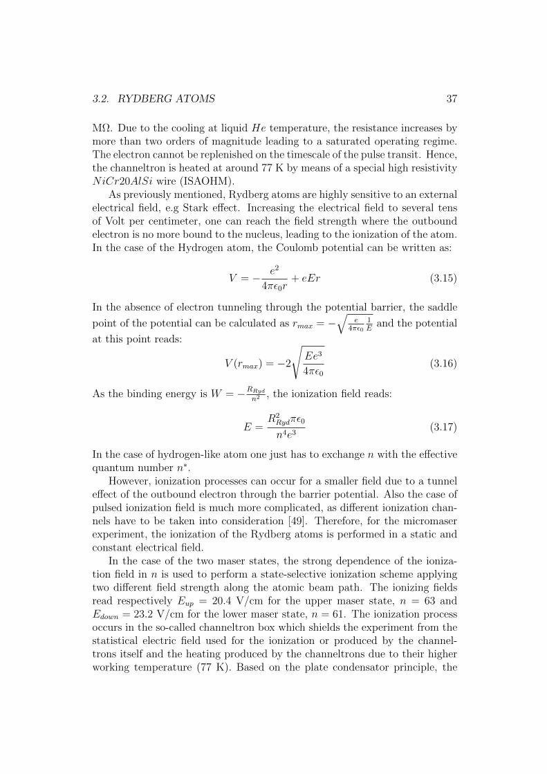
In the case of the two maser states, the strong dependence of the ioniza-tion field in n is used to perform a state-selective ionization scheme applyingtwo different field strength along the atomic beam path. The ionizing fieldsread respectively Eup = 20.4 V/cm for the upper maser state, n = 63 andEdown = 23.2 V/cm for the lower maser state, n = 61. The ionization processoccurs in the so-called channeltron box which shields the experiment from thestatistical electric field used for the ionization or produced by the channel-trons itself and the heating produced by the channeltrons due to their higherworking temperature (77 K). Based on the plate condensator principle, the
38 CHAPTER 3. EXPERIMENTAL SETUP
Positive charged grid
Channeltrons
Grounded slits for electric
field gradient shaping
Negative charged plate
Atomic beamAtomic beam
tV
ol
age
Position
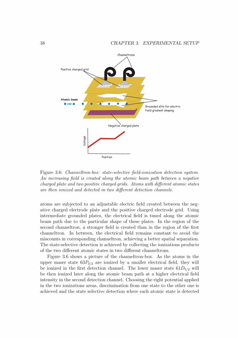
Figure 3.6: Channeltron-box: state-selective field-ionization detection system.An increasing field is created along the atomic beam path between a negativecharged plate and two positive charged grids. Atoms with different atomic statesare then ionized and detected in two different detection channels.
atoms are subjected to an adjustable electric field created between the neg-ative charged electrode plate and the positive charged electrode grid. Usingintermediate grounded plates, the electrical field is tuned along the atomicbeam path due to the particular shape of these plates. In the region of thesecond channeltron, a stronger field is created than in the region of the firstchanneltron. In between, the electrical field remains constant to avoid themiscounts in corresponding channeltron, achieving a better spatial separation.The state-selective detection is achieved by collecting the ionizations productsof the two different atomic states in two different channeltrons.
Figure 3.6 shows a picture of the channeltron-box. As the atoms in theupper maser state 63P3/2 are ionized by a smaller electrical field, they willbe ionized in the first detection channel. The lower maser state 61D5/2 willbe then ionized later along the atomic beam path at a higher electrical fieldintensity in the second detection channel. Choosing the right potential appliedin the two ionizations areas, discrimination from one state to the other one isachieved and the state selective detection where each atomic state is detected
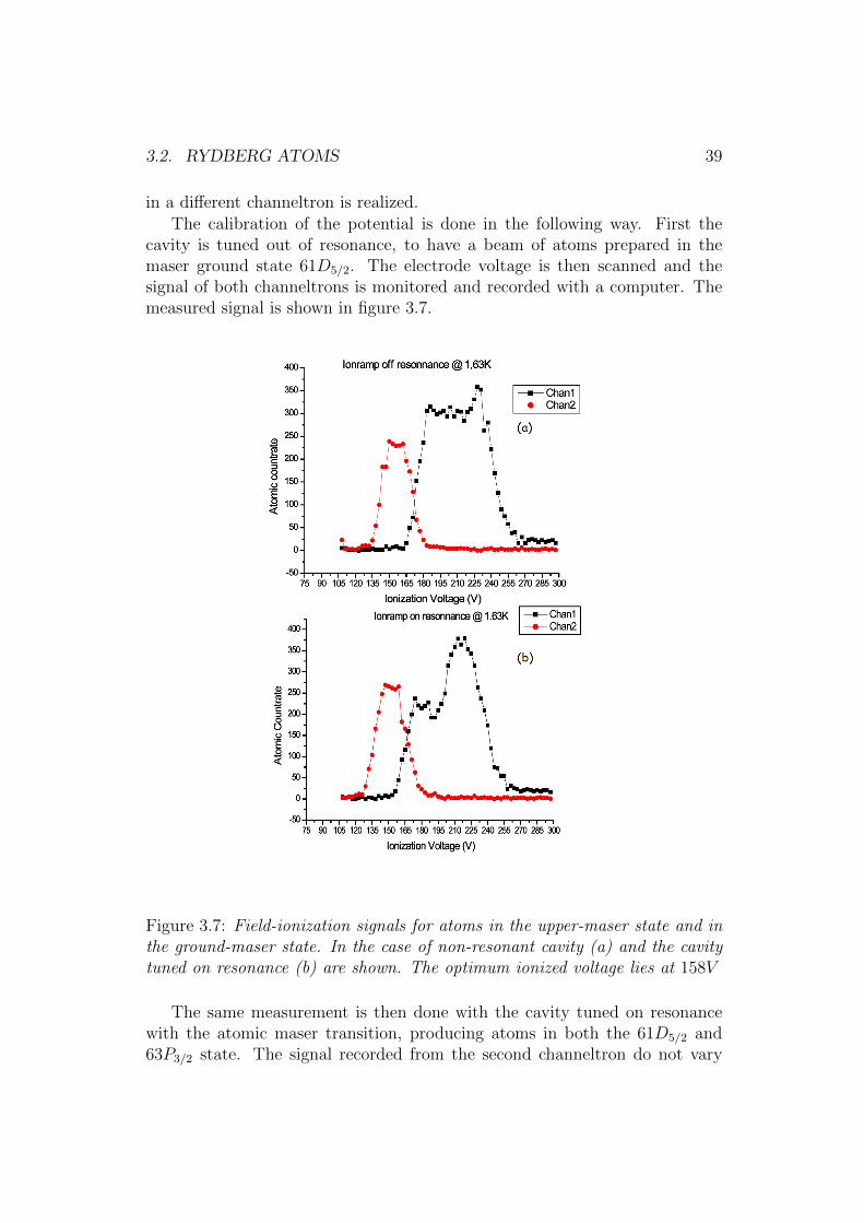
3.2. RYDBERG ATOMS 39
in a different channeltron is realized.The calibration of the potential is done in the following way. First the
cavity is tuned out of resonance, to have a beam of atoms prepared in themaser ground state 61D5/2. The electrode voltage is then scanned and thesignal of both channeltrons is monitored and recorded with a computer. Themeasured signal is shown in figure 3.7.
Figure 3.7: Field-ionization signals for atoms in the upper-maser state and inthe ground-maser state. In the case of non-resonant cavity (a) and the cavitytuned on resonance (b) are shown. The optimum ionized voltage lies at 158V
The same measurement is then done with the cavity tuned on resonancewith the atomic maser transition, producing atoms in both the 61D5/2 and63P3/2 state. The signal recorded from the second channeltron do not vary
40 CHAPTER 3. EXPERIMENTAL SETUP
corresponding to the maser ground state atoms ionized in the second detectionchannel until the electrical field is high enough in the first channel to ionize themaser ground state. However the signal collected from the first channeltronvaries from the non-resonant case to the resonant one. When no excited statesare produced (cavity off-resonance), the signal recorded in the first channeltroncorresponds to all ground states atoms ionized. Also, the curves recordedfrom the two channeltrons do not overlap showing that practically no groundstates atoms are detected in the first channeltron and the second one at thesame voltage. When the cavity is on resonance, the curve of channeltron1is shifted to a lower potential corresponding to the detection of atoms inthe excited maser state, reflecting the lower ionization potential of the 63P3/2
state. The slope of the curve also changes showing a step profile. The firstplateau corresponds to the detection of the excited states atoms while thesecond plateau corresponds to the detection of all atoms without any stateselection.
The optimum value of the applied ionization voltage lies where in the firstchanneltron the maximum of excited maser state are detected and at the sametime a minimal of maser ground state . Analogously for the second channeltronwhere the maximal of ground states atoms are detected with a minimum ofexcited states. The optimum values in this case lies at 158 V. This value ishigher than the theoretical one presented earlier. However one has to takeinto consideration the particular design of the channeltron box, with the twoground plates forming the field gradient and the distance of 2 cm between thetwo charged electrodes.
For the laser stabilization a much simpler ionization set-up is used as nostate selective detection is needed. Placed in an auxiliary chamber, a smallpart of the atomic beam interacts after collimation with the laser radiationand is excited into the maser ground state 61D5/2. The atoms are then ionizedin an orthogonal static electrical field produced by a tilted negative-potentialionization plate, producing an increasing field along the atomic beam path.This allows to keep a narrow zone of the ionization region and put the atomsin a linear electrical field ramp, avoiding the abrupt turn on of the ionizationfield corresponding to a pulsed electrical field. The signal detected is thendigitally processed to lock the second step laser onto the maximum of thespectroscopic signal.
In the excitation region, a small electrical field can also be produced withtwo parallel condensator plates. Shifting the atomic frequency due to the Starkeffect. This precisely controlled laser frequency shifting is then used to per-form a velocity selection of the atom and will be described in more details inChapter 4.

3.3. CAVITY 41
3.3 Cavity
For the generation and storage of the quantum light field, a superconductivecavity, developed and manufactured at the Max Planck for Quantum Optics,is used [60].
1 20 3cm
Figure 3.8: The high Q-factor superconductive niobium cavity used in the mi-cromaser experiment
The microwave cavity has a cylindrical form with a length and a diameterof about 25 mm. At the centers the presence of two holes with a 2 mm apertureallows the atomic beam to enter and exit the cavity as also the injection of anexternal microwave field.
Along the atomic beam axis, only the TE1np modes have a non vanishingtransversal electric field. In the case of the micromaser experiment, the Ryd-berg atoms interact with the TE121 mode. The mode form corresponds to ahalf period of a sine wave. Also, the polarization direction allows an externalcoherent field injection via a simple microwave coupling through an externalwaveguide. This is important, first for the cavity frequency and the Q-factormeasurements, and in the case of experiments requiring coherent states like thestudy of the phase diffusion process. The resonance frequency of a cylindricalcavity is given by [61]:
ω = c
√x′212
R2+π2
L2(3.18)
where R and L are the radius and length of the cavity respectively and x′12 is
the 2-nd zero of the first derivative of the Bessel function J1.
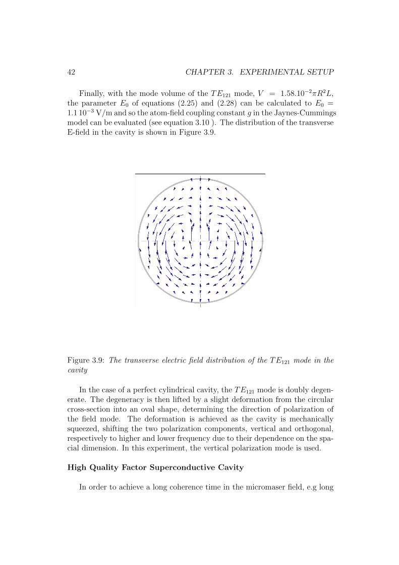
42 CHAPTER 3. EXPERIMENTAL SETUP
Finally, with the mode volume of the TE121 mode, V = 1.58.10−2πR2L,the parameter E0 of equations (2.25) and (2.28) can be calculated to E0 =1.1 10−3 V/m and so the atom-field coupling constant g in the Jaynes-Cummingsmodel can be evaluated (see equation 3.10 ). The distribution of the transverseE-field in the cavity is shown in Figure 3.9.
Figure 3.9: The transverse electric field distribution of the TE121 mode in thecavity
In the case of a perfect cylindrical cavity, the TE121 mode is doubly degen-erate. The degeneracy is then lifted by a slight deformation from the circularcross-section into an oval shape, determining the direction of polarization ofthe field mode. The deformation is achieved as the cavity is mechanicallysqueezed, shifting the two polarization components, vertical and orthogonal,respectively to higher and lower frequency due to their dependence on the spa-cial dimension. In this experiment, the vertical polarization mode is used.
High Quality Factor Superconductive Cavity
In order to achieve a long coherence time in the micromaser field, e.g long
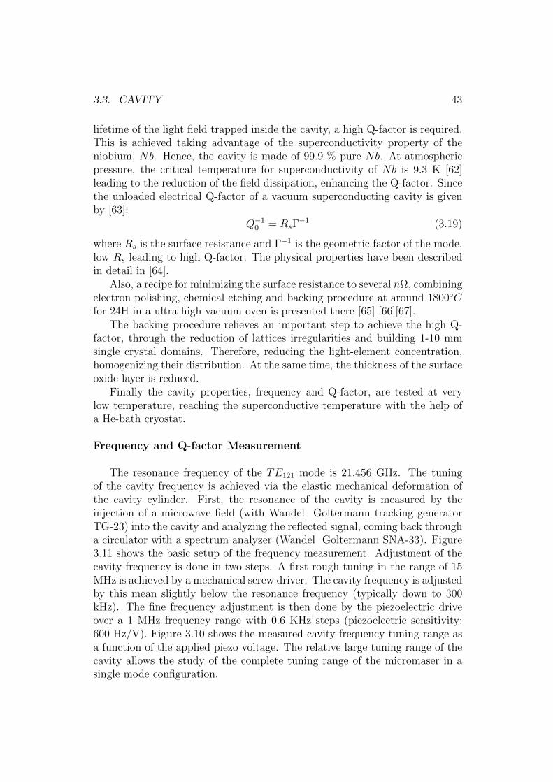
3.3. CAVITY 43
lifetime of the light field trapped inside the cavity, a high Q-factor is required.This is achieved taking advantage of the superconductivity property of theniobium, Nb. Hence, the cavity is made of 99.9 % pure Nb. At atmosphericpressure, the critical temperature for superconductivity of Nb is 9.3 K [62]leading to the reduction of the field dissipation, enhancing the Q-factor. Sincethe unloaded electrical Q-factor of a vacuum superconducting cavity is givenby [63]:
Q−10 = RsΓ
−1 (3.19)
where Rs is the surface resistance and Γ−1 is the geometric factor of the mode,low Rs leading to high Q-factor. The physical properties have been describedin detail in [64].
Also, a recipe for minimizing the surface resistance to several nΩ, combiningelectron polishing, chemical etching and backing procedure at around 1800Cfor 24H in a ultra high vacuum oven is presented there [65] [66][67].
The backing procedure relieves an important step to achieve the high Q-factor, through the reduction of lattices irregularities and building 1-10 mmsingle crystal domains. Therefore, reducing the light-element concentration,homogenizing their distribution. At the same time, the thickness of the surfaceoxide layer is reduced.
Finally the cavity properties, frequency and Q-factor, are tested at verylow temperature, reaching the superconductive temperature with the help ofa He-bath cryostat.
Frequency and Q-factor Measurement
The resonance frequency of the TE121 mode is 21.456 GHz. The tuningof the cavity frequency is achieved via the elastic mechanical deformation ofthe cavity cylinder. First, the resonance of the cavity is measured by theinjection of a microwave field (with Wandel Goltermann tracking generatorTG-23) into the cavity and analyzing the reflected signal, coming back througha circulator with a spectrum analyzer (Wandel Goltermann SNA-33). Figure3.11 shows the basic setup of the frequency measurement. Adjustment of thecavity frequency is done in two steps. A first rough tuning in the range of 15MHz is achieved by a mechanical screw driver. The cavity frequency is adjustedby this mean slightly below the resonance frequency (typically down to 300kHz). The fine frequency adjustment is then done by the piezoelectric driveover a 1 MHz frequency range with 0.6 KHz steps (piezoelectric sensitivity:600 Hz/V). Figure 3.10 shows the measured cavity frequency tuning range asa function of the applied piezo voltage. The relative large tuning range of thecavity allows the study of the complete tuning range of the micromaser in asingle mode configuration.
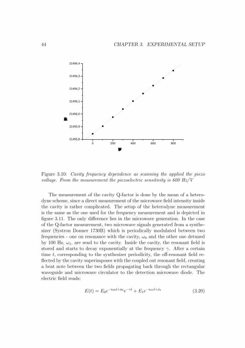
44 CHAPTER 3. EXPERIMENTAL SETUP
0 200 400 600 80021455,8
21455,9
21456,0
21456,1
21456,2
21456,3
21456,4C
avi
ty F
req
ue
ncy
(kH
z)
Piezzo Voltage U (V)
Figure 3.10: Cavity frequency dependence as scanning the applied the piezovoltage. From the measurement the piezoelectric sensitivity is 600 Hz/V
The measurement of the cavity Q-factor is done by the mean of a hetero-dyne scheme, since a direct measurement of the microwave field intensity insidethe cavity is rather complicated. The setup of the heterodyne measurementis the same as the one used for the frequency measurement and is depicted infigure 3.11. The only difference lies in the microwave generation. In the caseof the Q-factor measurement, two microwave signals generated from a synthe-sizer (Systron Donner 1730B) which is periodically modulated between twofrequencies - one on resonance with the cavity, ω0 and the other one detunedby 100 Hz, ω1, are send to the cavity. Inside the cavity, the resonant field isstored and starts to decay exponentially at the frequency γ. After a certaintime t, corresponding to the synthesizer periodicity, the off-resonant field re-flected by the cavity superimposes with the coupled out resonant field, creatinga beat note between the two fields propagating back through the rectangularwaveguide and microwave circulator to the detection microwave diode. Theelectric field reads:
E(t) = E0e−iω0t+φ0e−γt + E1e
−iω1t+φ1 (3.20)
3.3. CAVITY 45
Cavity
Amplifier
MW Synthesizer
Amplifier
DetectorOscilloscope
MW circulator
Figure 3.11: Frequency and Q-factor measurement setup.
Using a high pass filter, the strong reflected signal |E1|2 is filterd out andthe detected beat note signal is then proportional to:
|E(t)|2 ∝ 2E0E1cos[(ω0 − ω1)t+ φ0 − φ1]e−γt (3.21)
This shows that the beat signal decays with the same time constant as thecavity decay time. Measuring the decay time of the beat signal amplitudegives a direct measurement of the cavity photon lifetime, the cavity Q-factor:
Q = ω0τf =ω0
γ(3.22)
where τf is the cavity decay time.Figure 3.12 shows a typical result of such a heterodyne measurement. Cor-
responding to a decay time of 73 ms, extracted from the fit, the cavity Q-factoris Q = 4.9 109.
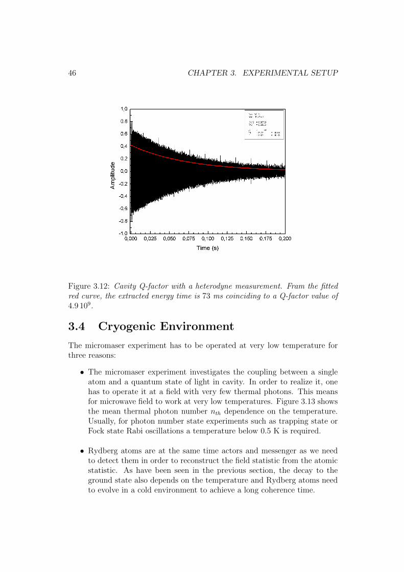
46 CHAPTER 3. EXPERIMENTAL SETUP
Figure 3.12: Cavity Q-factor with a heterodyne measurement. Fram the fittedred curve, the extracted energy time is 73 ms coinciding to a Q-factor value of4.9 109.
3.4 Cryogenic Environment
The micromaser experiment has to be operated at very low temperature forthree reasons:
• The micromaser experiment investigates the coupling between a singleatom and a quantum state of light in cavity. In order to realize it, onehas to operate it at a field with very few thermal photons. This meansfor microwave field to work at very low temperatures. Figure 3.13 showsthe mean thermal photon number nth dependence on the temperature.Usually, for photon number state experiments such as trapping state orFock state Rabi oscillations a temperature below 0.5 K is required.
• Rydberg atoms are at the same time actors and messenger as we needto detect them in order to reconstruct the field statistic from the atomicstatistic. As have been seen in the previous section, the decay to theground state also depends on the temperature and Rydberg atoms needto evolve in a cold environment to achieve a long coherence time.
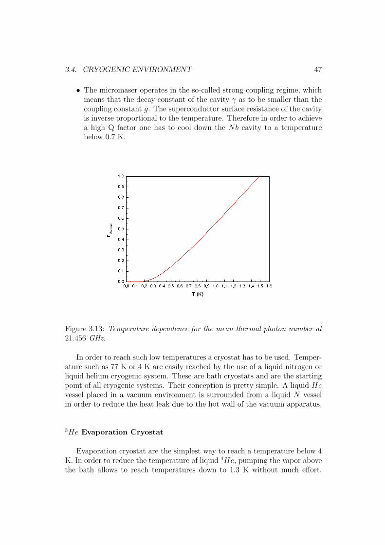
3.4. CRYOGENIC ENVIRONMENT 47
• The micromaser operates in the so-called strong coupling regime, whichmeans that the decay constant of the cavity γ as to be smaller than thecoupling constant g. The superconductor surface resistance of the cavityis inverse proportional to the temperature. Therefore in order to achievea high Q factor one has to cool down the Nb cavity to a temperaturebelow 0.7 K.
Figure 3.13: Temperature dependence for the mean thermal photon number at21.456 GHz.
In order to reach such low temperatures a cryostat has to be used. Temper-ature such as 77 K or 4 K are easily reached by the use of a liquid nitrogen orliquid helium cryogenic system. These are bath cryostats and are the startingpoint of all cryogenic systems. Their conception is pretty simple. A liquid Hevessel placed in a vacuum environment is surrounded from a liquid N vesselin order to reduce the heat leak due to the hot wall of the vacuum apparatus.
3He Evaporation Cryostat
Evaporation cryostat are the simplest way to reach a temperature below 4K. In order to reduce the temperature of liquid 4He, pumping the vapor abovethe bath allows to reach temperatures down to 1.3 K without much effort.
48 CHAPTER 3. EXPERIMENTAL SETUP
But it is not sufficient for our purpose. With a 3He evaporation cryostat itis possible to reach lower temperature[68]. The use of 3He has two essentialadvantages over 4He. First the higher vapor pressure allows temperatures aslow as 0.3 K. Secondly, 3He does not possess the problem created by creepingsuperfluid film, which lead to an enhancement of the heat transport from thewarm part to the cold part.
A special designed Oxford 3He is used and has been described in detailsin [30]. A nitrogen bath at 77 K and a 4He bath at 4 K surround a vac-uum chamber. In the center of this chamber is placen the 3He pot (so calledcold-finger) on which the main part of the experimental set-up, cavity witha microwave coupler, piezo system for cavity squeezing and the collimator, ismounted. To pre-cool the system a 4He evaporation cryostat is used. Theso-called 1K pot is connected to the main 4He bath with the help of a narrowtube ( about 1 mm diameter). A needle valve controls precisely the liquid4He flow from the main bath. The 4He is mechanically pumped to reach atemperature of 1.3K . The 1K pot then plays the role of a heat sink. At thistemperature, the 3He gas starts to condense in the 3He pot. Once all the 3Heis condensed, reaching a temperature around 0.9 K one can start to pump it.The pumping is done via an absorption pump. In this case, the 3He that iscondensed inside the cold-finger is absorbed onto charcoal powder. While thisoperation, this absorption pump is cooled down below 40K by anchoring it atthe 4He main bath. Because of the large surface area of the charcoal pump,the 3He is pumped in a very efficient way. The reduction pressure allows toreach a working temperature of 300 mK for a 12 hours cycling time. After the3He is pumped and the cold-finger is empty the absorption pump is warmingup. Upon warming, the 3He is desorbed. The 3He gas is pumped back in thedumps for storage or can be re-condensed for a new cooling cycle.
3He−4 He Dilution Cryostat
In the previous section, we discussed the cooling process of a liquid bypumping the vapor above it. Using 3He, the lowest temperature that has beenachieved is 0.24 K [69], where in our system the end working temperatureis around 300 mK. In order to reach lower temperature, one has to use thespecific thermodynamical properties of dilute 3He −4 He mixture. The basicidea of this method was first introduced by London in 1951 [70] .
The principle operation of a dilution refrigerator is based on the fact that aphase separation in 3He−4He mixtures occurs at very low temperature. First,because 4He atoms, due to their larger mass, have a lower zero-point energy,the 3He atoms are more strongly bound to them than among each other.Secondly, the 3He atoms obey to the Fermi statistics and thus their kinetic
3.4. CRYOGENIC ENVIRONMENT 49
energy increases with their number density, which leads to the reduction of thebinding energy. Already at a 3He concentration of 6.5% in 4He, the bindingenergy vanishes when T → 0 and no 3He can be dissolved in the 4He and aphase separation occurs. A light, 3He rich phase and a heavy 4He phase areproduced. In the dilution cryostat performed in Garching, a 3He concentrationof around 25% is used. This is energetically more favorable for the two phases.
The heart of the dilution refrigerator is the so-called mixing chamber wherethe transfer of 3He from the light phase into the dilute one occurs. As the 3Heatoms in the 3He rich phase have a lower entropy than the rest 3He atoms inthe heavy 4He phase, the transfer of 3He atoms from one phase to the otherleads to a cooling of the mixture. In analogy to evaporation of gases, one canunderstand this process as an evaporation of 3He atoms into the quasi-vacuumof the superfluid 4He. In order to use this cooling process in a continuous waya new phase separation occurs where 3He atoms are extracted from the dilutephase and re-inject in the 3He rich phase.
Figure 3.14 shows a scheme of the dilution cryostat used to perform themicromaser experiment. The 3He−4He circuit is sitting in a vacuum chamberimmersed in a 4He bath. As for the 3He cryostat the 3He −4 He mixture iscondensed with the help of a so-called 1K pot. The cavity is directly mountedon the mixing chamber which is the coldest part of the dilution cryostat. The3He −4 He circuit consists essentially of the mixing chamber, the still anda counter flow heat exchanger. This circuit has to realize a sufficiently highcirculation of 3He, while maintaining the heat load at the mixing chamberas low as possible. The circulation of the 3He atoms is driven by pumpingthe still. The still is heated at around 0.7 K so that at this point a phaseseparation between the 3He atoms and the 4He atoms occurs. Due to theirhigher vapor pressure, most of the 3He atoms are evaporated and pumpedout. After cleaning in nitrogen and liquid helium traps, the 3He atoms are re-injected in the cooling circuit and again pre-cooled in the 1 K pot. After the 1K pot, as the pressure is sufficiently high, 3He atoms condense before enteringthe counterflow heat exchanger system. this consists in two different typesof heat exchangers. The first type, the so-called continuous heat exchanger iscomposed of two tubes that are mounted in a such complicated way so that theinterface between the both is as large as possible to achieve a maximal thermalcontact. The second one, so called step heat exchanger, consists of severalchambers made from sintered silver in oder to increase the thermal contactarea. There, the phase separation occurs with the lighter 3He rich phaseforming the top layer. In the mixing chamber, 3He atoms are diffusing acrossthe phase boundary and are mixed to the quasi-stationary liquid 4He, whereadiabatic dilution causes the cooling. 3He atoms then diffuse back to the stillvia the heat exchanger where they will be evaporated. The lowest temperature
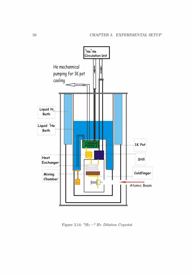
50 CHAPTER 3. EXPERIMENTAL SETUP
He- HeCirculation Unit
Liquid N
Bath
Liquid He
Bath
1K Pot
Still
Coldfinger
Heat
Exchanger
Mixing
Chamber
2
4
He mechannical
pumping for 1K pot
cooling
Atomic Beam
3 4
Figure 3.14: 3He−4 He Dilution Cryostat
3.4. CRYOGENIC ENVIRONMENT 51
obtained with a dilution cryostat is 1.5 mK [71]. In the micromaser experimentin Garching, the end working temperature is around 150 mK. This ”bad”performance is due to the large mass that has to be cooled,e.g cavity, piezossystem, and the outside heating due to the laser radiations, electrical wires,the close detection system at a 4 K temperature and the atomic oven. On theother hand a large improvement is done as the end working temperature wasimproved by adding a new shielding at 0.8 K and moreover, due to a bettercontrol over the still temperature a continuous working temperature rangefrom 1.3K down to 150 mK is accessible which is one of the requirements formeasuring quantum stochastic resonances in the micromaser [72].

52 CHAPTER 3. EXPERIMENTAL SETUP
Chapter 4
Experiments with MaserGround State Atoms
The first experiments with atoms in the maser ground state, the 61D5/2 Rydbergstate are presented. The magnetic field compensation using the Hanle effect isrealized for the first time in this configuration. Earth magnetic field avoids thedegeneracy of the mj components of the Rydberg states and therefore, needsto be compensated at the mG level. The Stark effect of the Rydberg 61D5/2
state is investigated. The Stark effect is used in the micromaser experiment toperform a velocity section of the atoms, controlling their interaction time withthe cavity field via the Doppler effect. Finally, the first maser experiments,where ground state atoms interact with the quantized thermal field of the cav-ity are performed. In particular, Rabi oscillations with a very high contrast areobserved, performing a direct measurement of the field temperature.
In Chapter two, the Jaynes-Cummings model describing the interactionbetween a two-level system and a single radiation mode of a cavity has beenintroduced. The realization of a very high-Q cavity with a long trapping timeof the radiation field, and the large dipole interaction between two Rydbergstates lead to the strong coupling regime where the coherent interaction isdominant. Cavity QED experiments with Rydberg atoms offer therefore awide range of experimental conditions to study the light-matter interaction atthe quantum level with a single atom.
The one-atom-maser or micromaser is a system where a stream of atomsinteracts one by one with the cavity field. For a low atomic injection rate, withless than one atom per cavity decay time, the realization of Rabi oscillationsbetween a nonclassical field and the two-level Rydberg system is possible. Fora larger atomic pumping, the combination of the coherent interaction anddecay processes leads to a steady-state of the field, analogous to a laser or a
53
54CHAPTER 4. EXPERIMENTSWITHMASERGROUND STATE ATOMS
maser. Due to the strong coupling, the presence of only one atom in the cavityis a sufficient condition to achieve stimulated emission. In the steady-state,the generation of a non classical field with sub-Poissonian statistics is possible.Finally, due to the long coherence time of the system, one atom can experiencethe field in the cavity created through the interaction between the cavity andthe previous atoms opening a path towards atomic entanglement controlled bythe coherent interaction with the cavity field [73].
In the following sections, the magnetic field compensation will be explained.This is necessary as the earth magnetic field affects the micromaser experimenton two aspects: the magnetic sub-levels are no more degenerated and an exter-nal field affects the the high Q factor of the cavity. Then, the velocity selectionof the atoms and the control of the interaction time will be developed. Finally,the first experiments between ground states atoms and the quantized thermalfield of the cavity are presented. The experiments are performed, both forlarge atomic pumping with the measurement of the so-called maser line andfor low atomic injection rate where informations about the actual field temper-ature are extracted from the measurement of Rabi oscillations between groundstates atoms and the cavity field at thermal equilibrium.
4.1 Magnetic Field Compensation
The earth magnetic field and the electronic components present in the ex-perimental environment contribute to a non zero magnetic field in the exper-imental region of the order of 350 mG. This residual magnetic field has tobe compensated due to its influence on the micromaser experiment. First,in the presence of an external magnetic field, the magnetic sublevels of the63P1/2 and 61D5/2 are no longer degenerate. The different Lande-factors ofthe mj = +1/2 ↔ +1/2 and mj = −1/2 ↔ −1/2 transitions lead to a split-ting of about 1.5 kHz/mG. Since the splitting should be smaller than the Rabifrequency Ω/2π ≈ 7, 2 kHz, the magnetic field should be compensated at themG level [74].
Another reason for the compensation lies in the cavity properties itself.Since the cavity is made from niobium, which is a superconductor of typeII, below the superconductive critical temperature (9.3 K), the magnetic fieldfluxes freeze inside the material, increasing the high frequency resistance [75] ofthe cavity walls. The Q-factor is then degraded [76], leading to the reductionof the lifetime τcav of the field.
The all experimental setup is made of niobium which is a superconductorof type II and the compensation can be done only once before cooling down toliquid He temperature. Once the compensation is achieved and the cavity iscooled down below the superconductive temperature of 9.3 K, the zero mag-
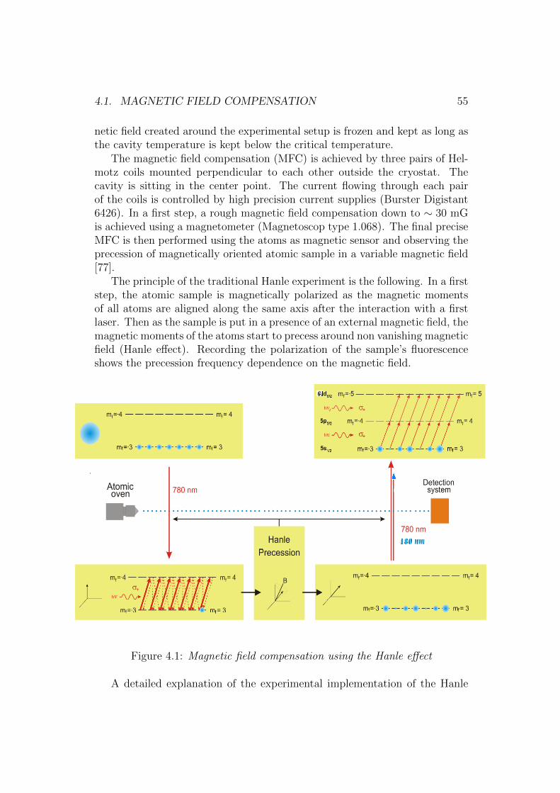
4.1. MAGNETIC FIELD COMPENSATION 55
netic field created around the experimental setup is frozen and kept as long asthe cavity temperature is kept below the critical temperature.
The magnetic field compensation (MFC) is achieved by three pairs of Hel-motz coils mounted perpendicular to each other outside the cryostat. Thecavity is sitting in the center point. The current flowing through each pairof the coils is controlled by high precision current supplies (Burster Digistant6426). In a first step, a rough magnetic field compensation down to ∼ 30 mGis achieved using a magnetometer (Magnetoscop type 1.068). The final preciseMFC is then performed using the atoms as magnetic sensor and observing theprecession of magnetically oriented atomic sample in a variable magnetic field[77].
The principle of the traditional Hanle experiment is the following. In a firststep, the atomic sample is magnetically polarized as the magnetic momentsof all atoms are aligned along the same axis after the interaction with a firstlaser. Then as the sample is put in a presence of an external magnetic field, themagnetic moments of the atoms start to precess around non vanishing magneticfield (Hanle effect). Recording the polarization of the sample’s fluorescenceshows the precession frequency dependence on the magnetic field.
Figure 4.1: Magnetic field compensation using the Hanle effect
A detailed explanation of the experimental implementation of the Hanle

56CHAPTER 4. EXPERIMENTSWITHMASERGROUND STATE ATOMS
effect measurement in the micromaser is shown in figure 4.1. Atoms emergingfrom the oven are in equally distributed quantum states over all mf magneticsub-levels. Using the hyperfine transition of the Rb D2 line at 780 nm:
52S1/2, F = 3↔ 52P3/2, F = 4 (4.1)
and applying a circular polarized laser light it is possible to optically pumpthe atoms in a well-defined magnetic sub-level mf . Since only the transitionsof δmf = +1 are allowed, after several hundred of absorption and sponta-neous emission cycles the atoms are prepared in the quantum ground state52S1/2, F = 3,mf = 3 with well aligned magnetic moments.
Then, the atoms are placed in a static homogeneous magnetic field duringa certain time t, corresponding to the time of flight of the atoms from the firstlaser excitation region where the optical pumping occurs to the second laserexcitation region where the atoms are exited into a well defined Rydberg state.
The magnetic moment of the atom precesses around the magnetic field,thereby changing coherently the distribution of themf quantum number states.The probability that the spin of the atom will be oriented in the initial direction(mf = +3) after a time t is given by:
Pmf=+3(t) = 1− sin2(α) sin2(ωt) (4.2)
where α is the angle between the magnetic field and the laser beam, deter-mining the quantization axis, and ω = gF
eB2m
is the Larmor frequency and gFthe hyperfine structure Lande-factor (here 1/3). From equation 4.2, in thespecial case where the laser and the magnetic field are aligned, no precessionoccurs. The atoms magnetic moments and the magnetic field are collinear andthe atoms remains in the mf = +3 state. One can also note, if the interactionis fully coherent, one cannot speak strictly of magnetic coherent control overthe magnetic level as only the mf = +3 state is well defined over the interac-tion time as the distribution over the others mf states remains uncontrolled.The mF states can only be distributed corresponding to the orientation of theclassical B field.
Finally, the atoms are excited to the 61D5/2 Rydberg state with a two-steps laser excitation scheme. The polarizations of the two lasers (σ+, σ+) arechosen so that in a zero magnetic field, the excitation rate over the ladder:
5S1/2, F = 3,mf = +3→ 5P3/2, F = 4,mf = +4→ 61D5/2, F = 5,mf = +5(4.3)
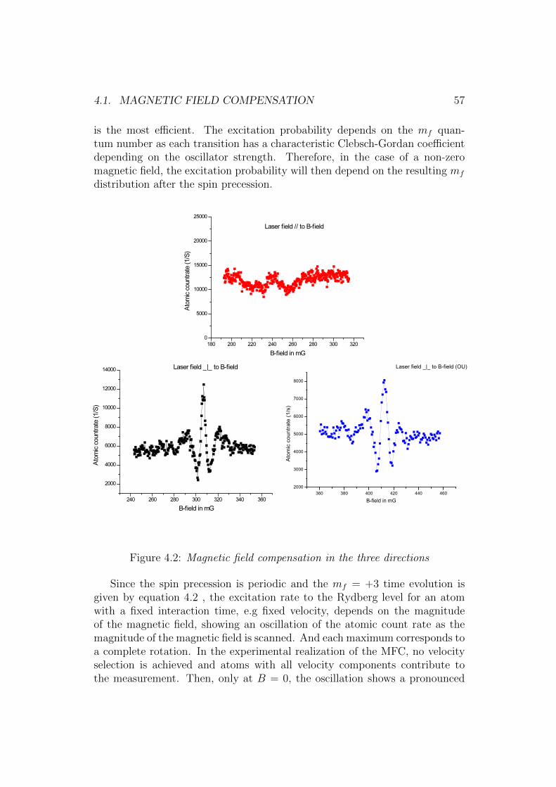
4.1. MAGNETIC FIELD COMPENSATION 57
is the most efficient. The excitation probability depends on the mf quan-tum number as each transition has a characteristic Clebsch-Gordan coefficientdepending on the oscillator strength. Therefore, in the case of a non-zeromagnetic field, the excitation probability will then depend on the resulting mf
distribution after the spin precession.
360 380 400 420 440 4602000
3000
4000
5000
6000
7000
8000
Laser field _|_ to B-field (OU)
B-field in mG
Ato
mic
cou
ntra
te (1
/s)
Figure 4.2: Magnetic field compensation in the three directions
Since the spin precession is periodic and the mf = +3 time evolution isgiven by equation 4.2 , the excitation rate to the Rydberg level for an atomwith a fixed interaction time, e.g fixed velocity, depends on the magnitudeof the magnetic field, showing an oscillation of the atomic count rate as themagnitude of the magnetic field is scanned. And each maximum corresponds toa complete rotation. In the experimental realization of the MFC, no velocityselection is achieved and atoms with all velocity components contribute tothe measurement. Then, only at B = 0, the oscillation shows a pronounced

58CHAPTER 4. EXPERIMENTSWITHMASERGROUND STATE ATOMS
maximum, since no rotation occurs and the magnetic moment remains aligned.However, a symmetric oscillating pattern along one defined axis (x-axis
for example) is only achieved if the other field component (y- and z-axis) arecompensated to zero. An iterative method in all three direction is used toperform the MFC. Concerning the particular case, when the magnetic fieldand the laser are collinear, the zero-field point measurement is achieved byapplying a small off-set field (∼ 3 mG) in one of the other directions.
Figure 4.2 shows the experimental result of the magnetic field compensationin the micromaser achieved with the detection of the 61D5/2 Rydberg state.The right compensating magnetic field is determined from the maximum atthe symmetry center of the curve. And a magnetic field compensation with aprecision on the order of 1 mG is achieved.
MFC measurements have been developed since the very beginning of themicromaser experiments. But the detection scheme using the micromaserground state, e.g 61D5/2 Rydberg state shows improvements in the fringe con-trast, due to the Clebsch-Gordan coefficients of the 2nd step laser with σ+
polarization for the 5P3/2, F = 4 → 61D5/2, F = 5 transition, compared toprevious measurements [78, 79].
4.2 Stark Effect and Velocity Selection by Doppler
Effect
In chapter 2, the central equation determining the micromaser steady-state isderived and reads:
ρssnn = ρss00
n∏k=1
nthγ + Ek(nth + 1)γ + Gk
(4.4)
with the Rabi dynamics contribution:
Ek =Re
ksin2(√kgτ) (4.5)
Gk =Rg
ksin2(√kgτ) (4.6)
The mean thermal field photon number nth is determined by the cavitytemperature, and the pumping rate is controlled by the laser excitation rate,e.g laser field intensity. The third experimental parameter, the interactiontime is optically controlled via the Doppler effect and will be the subject ofthis section.
Accurate control of the interaction time between atoms and field plays animportant role in the micromaser dynamics as it gives access to different quan-tum features of the produced field such as sub-poissonian field, trapping states
4.2. STARK EFFECT ANDVELOCITY SELECTION BYDOPPLER EFFECT 59
or bistability. In the case of the micromaser, since the cavity mode is ori-ented along the atomic beam axis, the interaction time is equal to the transitflight time of the atoms inside the cavity. The interaction time control hasbeen achieved by different technics over the different experiments, presentingadvantages and disadvantages. The first technique used was the mechanicalvelocity selection by means of nine Fizeau wheels. The main advantage is thevery accurate selection with a interaction time spreading smaller than 4% [38].On the other hand, the mechanical cut of the atomic beam strongly reducesthe atomic flux.
Doppler Velocity Selection
The optical velocity selection of the atoms is achieved using Doppler ef-fect via the angular excitation of the atoms. This allows the selection of asub-velocity class among all velocities available in the thermal atomic beam.The Doppler selection is achieved using the angular excitation of the Rydbergatoms. The Rydberg excitation to the micromaser ground state, 61D5/2, isachieved by means of a two-step excitation scheme. The first laser step, pro-moting the 85Rb atoms to the 5P3/2, F = 4 state is doppler free and interactsperpendicularly to the atomic beam. The Doppler selection is achieved as thesecond step laser at 480 nm interacts with the atomic beam at the same pointas the first step but at an angle of 11. Due to the angular excitation, theatoms see a Doppler shifted laser light, with the frequency:
ν ′ = νlc+ v sin θ
c= νl
(1 +
v sin θ
c
)(4.7)
where νl is the blue laser frequency, v the atoms velocity and θ the anglebetween the atomic beam and the laser light field, as c is the speed of light.It is therefore possible to select a certain velocity class of atoms by tuning thelaser frequency as:
v =c∆ν
νl sin θ(4.8)
where ν is the atomic transition, 5P3/2, F = 4→ 61D5/2, frequency and∆ν = ν − νl. The accuracy of the velocity selection depends on several ex-perimental parameters. The atomic divergence is reduced as the atomic beamis collimated (see Chapter 3). Other parameters are the laser frequency andlaser linewidth. Compared to the one step excitation in the UV, the blue laserfrequency is around 1.6 time smaller (297 nm compared to 480 nm) leadingto an enhancement in the uncertainty of the same order. This increase in un-certainty is however counterbalanced by a better linewidth of the blue laser
60CHAPTER 4. EXPERIMENTSWITHMASERGROUND STATE ATOMS
system, leading to a typically interaction time spreading δt/t of the order of 3%.
Laser Frequency Shift using the Stark Effect
In the previous chapter, the high sensitivity (or polarisability) of the Ry-dberg atoms due to an external electrical field E is explained and used forthe state-selective detection scheme. At very small fields on the order of sev-eral hundreds of mV/cm, energy shifts of the order of hundreds of MHz areobserved. Using the atomic frequency shift due to the Stark effect, the laserfrequency can be tuned for atomic velocity selection. The quadratic Starkeffect is the dominating term and the energy change W is given by:
W = −~αE2 (4.9)
where α, the polarisability, is state dependent. The polarisibility for the mi-cromaser excited state 63P3/2 has been experimentally determined as α =1482 ± 33 MHz/( V
cm)2 [80]. In some Rydberg states, measurements of the
Stark shifts and splittings at low electrical field strength show that the fa-miliar second order expansion is no longer adequate and deviations from thequadratic dependence are found [81, 82, 83]. The fourth-order Stark effect in-vestigations shows good agreement in the case of Ca Rydberg D states , givenan interpretation of the hyperpolarisabilities previously observed [84]. In thecase of the micromaser ground state, 61D5/2, the fourth-order contributionshas to be taken into account. The energy change W is then given by:
W = −~αE2 − ~γE4 (4.10)
where γ is the hyperpolarisability.The frequency locking of the Rydberg laser system (the U.V laser for the up-
per maser state, 63P3/2 and the blue laser for the maser ground state, 61D5/2)is achieved in the so-called auxiliary chamber, shown in figure 4.3. A smallfraction of the atomic beam, highly collimated, interacts with the laser light inpresence of an external electric field created between two parallel condensatorplates. At the end the Rydberg atoms are detected using the same field-ionization technique as described in Chapter 3. The laser is then locked on themaximum of the spectroscopy signal using a traditional lock-in demodulationtechnique. The frequency tuning is then controlled via the Stark voltage asthe spectral lines are shifted.
The second order shift is always to lower energy (redshift), as expected fromoscillator strength sum rules [85]. The Doppler shift can be either blueshiftedor redshifted depending on the relative angle θ between the light propagationand the atomic beam axis. For too large electrical fields, a splitting between
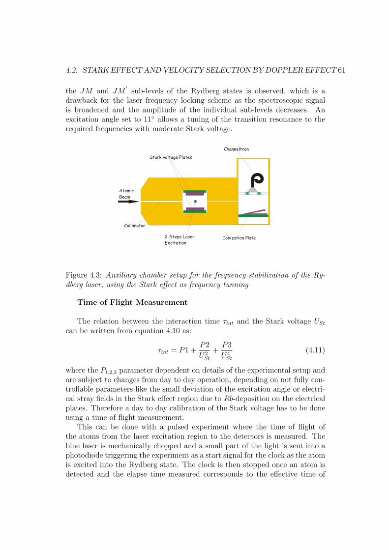
4.2. STARK EFFECT ANDVELOCITY SELECTION BYDOPPLER EFFECT 61
the JM and JM′
sub-levels of the Rydberg states is observed, which is adrawback for the laser frequency locking scheme as the spectroscopic signalis broadened and the amplitude of the individual sub-levels decreases. Anexcitation angle set to 11 allows a tuning of the transition resonance to therequired frequencies with moderate Stark voltage.
Stark voltage Plates
Atomic
Beam
Collimator
Ionization Plate
Channeltron
2-Steps Laser
Excitation
Figure 4.3: Auxiliary chamber setup for the frequency stabilization of the Ry-dberg laser, using the Stark effect as frequency tunning
Time of Flight Measurement
The relation between the interaction time τint and the Stark voltage UStcan be written from equation 4.10 as:
τint = P1 +P2
U2St
+P3
U4St
(4.11)
where the P1,2,3 parameter dependent on details of the experimental setup andare subject to changes from day to day operation, depending on not fully con-trollable parameters like the small deviation of the excitation angle or electri-cal stray fields in the Stark effect region due to Rb-deposition on the electricalplates. Therefore a day to day calibration of the Stark voltage has to be doneusing a time of flight measurement.
This can be done with a pulsed experiment where the time of flight ofthe atoms from the laser excitation region to the detectors is measured. Theblue laser is mechanically chopped and a small part of the light is sent into aphotodiode triggering the experiment as a start signal for the clock as the atomis excited into the Rydberg state. The clock is then stopped once an atom isdetected and the elapse time measured corresponds to the effective time of
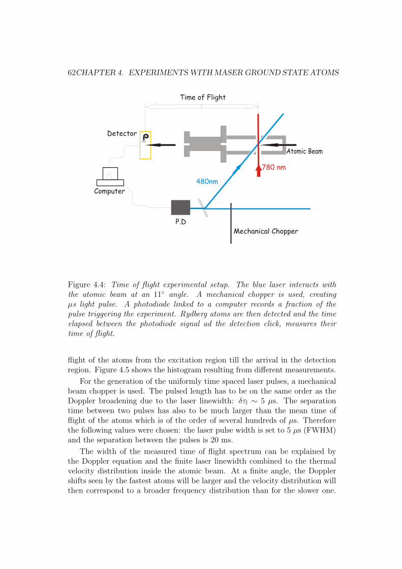
62CHAPTER 4. EXPERIMENTSWITHMASERGROUND STATE ATOMS
780 nm
480nm
Atomic Beam
P.D
Mechanical Chopper
Detector
Time of Flight
Computer
Figure 4.4: Time of flight experimental setup. The blue laser interacts withthe atomic beam at an 11 angle. A mechanical chopper is used, creatingµs light pulse. A photodiode linked to a computer records a fraction of thepulse triggering the experiment. Rydberg atoms are then detected and the timeelapsed between the photodiode signal ad the detection click, measures theirtime of flight.
flight of the atoms from the excitation region till the arrival in the detectionregion. Figure 4.5 shows the histogram resulting from different measurements.
For the generation of the uniformly time spaced laser pulses, a mechanicalbeam chopper is used. The pulsed length has to be on the same order as theDoppler broadening due to the laser linewidth: δτl ∼ 5 µs. The separationtime between two pulses has also to be much larger than the mean time offlight of the atoms which is of the order of several hundreds of µs. Thereforethe following values were chosen: the laser pulse width is set to 5 µs (FWHM)and the separation between the pulses is 20 ms.
The width of the measured time of flight spectrum can be explained bythe Doppler equation and the finite laser linewidth combined to the thermalvelocity distribution inside the atomic beam. At a finite angle, the Dopplershifts seen by the fastest atoms will be larger and the velocity distribution willthen correspond to a broader frequency distribution than for the slower one.
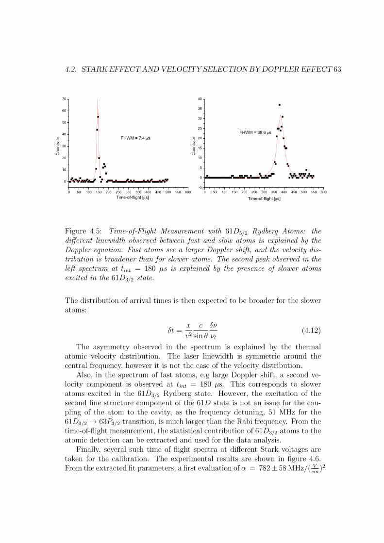
4.2. STARK EFFECT ANDVELOCITY SELECTION BYDOPPLER EFFECT 63
! "! #!! #"! $!! $"! %!! %"! &!! &"! "!! ""! '!!("
!
"
#!
#"
$!
$"
%!
%"
&!
)*+,-.-%/0'-!1
234567869
:;<9(3=(=>;?@6-A!1B! "! #!! #"! $!! $"! %!! %"! &!! &"! "!! ""! '!!
!
#!
$!
%!
&!
"!
'!
(!
)*+,-.-(/&-!0
123456757829:;-<!0=
>6?@;AB;4
Figure 4.5: Time-of-Flight Measurement with 61D5/2 Rydberg Atoms: thedifferent linewidth observed between fast and slow atoms is explained by theDoppler equation. Fast atoms see a larger Doppler shift, and the velocity dis-tribution is broadener than for slower atoms. The second peak observed in theleft spectrum at tint = 180 µs is explained by the presence of slower atomsexcited in the 61D3/2 state.
The distribution of arrival times is then expected to be broader for the sloweratoms:
δt =x
v2
c
sin θ
δν
νl(4.12)
The asymmetry observed in the spectrum is explained by the thermalatomic velocity distribution. The laser linewidth is symmetric around thecentral frequency, however it is not the case of the velocity distribution.
Also, in the spectrum of fast atoms, e.g large Doppler shift, a second ve-locity component is observed at tint = 180 µs. This corresponds to sloweratoms excited in the 61D3/2 Rydberg state. However, the excitation of thesecond fine structure component of the 61D state is not an issue for the cou-pling of the atom to the cavity, as the frequency detuning, 51 MHz for the61D3/2 → 63P3/2 transition, is much larger than the Rabi frequency. From thetime-of-flight measurement, the statistical contribution of 61D3/2 atoms to theatomic detection can be extracted and used for the data analysis.
Finally, several such time of flight spectra at different Stark voltages aretaken for the calibration. The experimental results are shown in figure 4.6.From the extracted fit parameters, a first evaluation of α = 782± 58 MHz/( V
cm)2
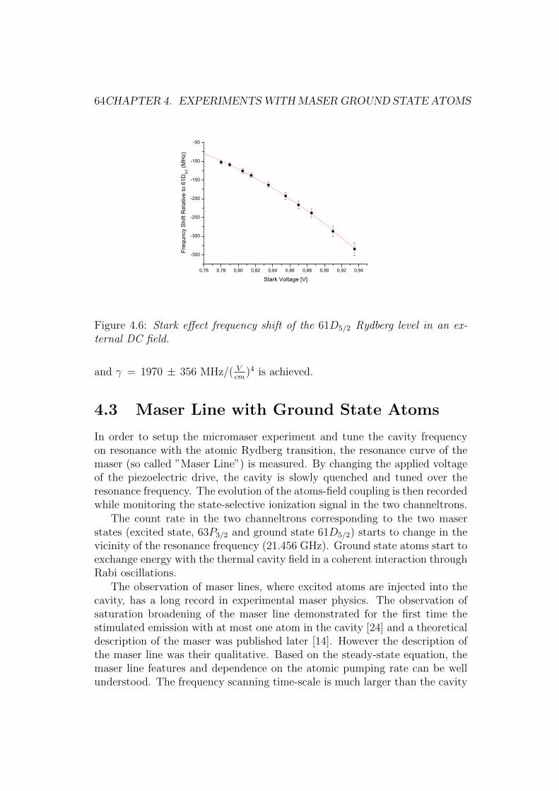
64CHAPTER 4. EXPERIMENTSWITHMASERGROUND STATE ATOMS
0,76 0,78 0,80 0,82 0,84 0,86 0,88 0,90 0,92 0,94
-350
-300
-250
-200
-150
-100
-50
Frequncy Shift Relative to 61D5/2 (MHz)
Stark Voltage [V]
Figure 4.6: Stark effect frequency shift of the 61D5/2 Rydberg level in an ex-ternal DC field.
and γ = 1970 ± 356 MHz/( Vcm
)4 is achieved.
4.3 Maser Line with Ground State Atoms
In order to setup the micromaser experiment and tune the cavity frequencyon resonance with the atomic Rydberg transition, the resonance curve of themaser (so called ”Maser Line”) is measured. By changing the applied voltageof the piezoelectric drive, the cavity is slowly quenched and tuned over theresonance frequency. The evolution of the atoms-field coupling is then recordedwhile monitoring the state-selective ionization signal in the two channeltrons.
The count rate in the two channeltrons corresponding to the two maserstates (excited state, 63P3/2 and ground state 61D5/2) starts to change in thevicinity of the resonance frequency (21.456 GHz). Ground state atoms start toexchange energy with the thermal cavity field in a coherent interaction throughRabi oscillations.
The observation of maser lines, where excited atoms are injected into thecavity, has a long record in experimental maser physics. The observation ofsaturation broadening of the maser line demonstrated for the first time thestimulated emission with at most one atom in the cavity [24] and a theoreticaldescription of the maser was published later [14]. However the description ofthe maser line was their qualitative. Based on the steady-state equation, themaser line features and dependence on the atomic pumping rate can be wellunderstood. The frequency scanning time-scale is much larger than the cavity
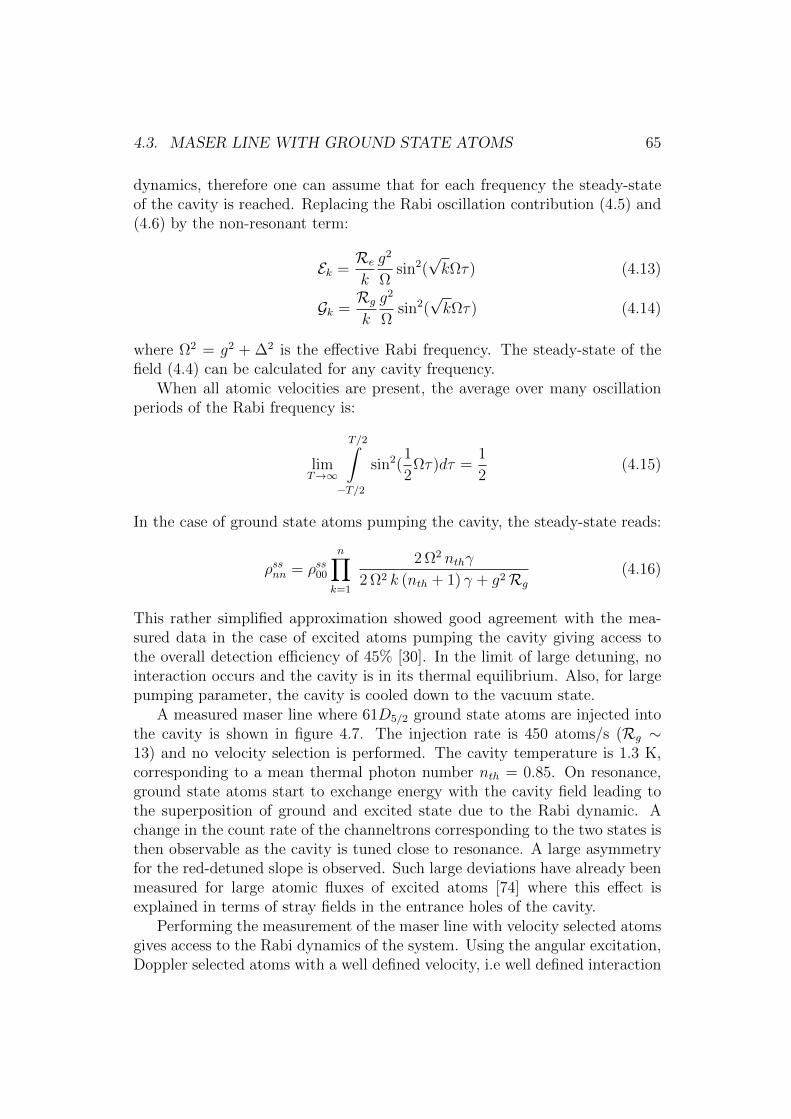
4.3. MASER LINE WITH GROUND STATE ATOMS 65
dynamics, therefore one can assume that for each frequency the steady-stateof the cavity is reached. Replacing the Rabi oscillation contribution (4.5) and(4.6) by the non-resonant term:
Ek =Re
k
g2
Ωsin2(√kΩτ) (4.13)
Gk =Rg
k
g2
Ωsin2(√kΩτ) (4.14)
where Ω2 = g2 + ∆2 is the effective Rabi frequency. The steady-state of thefield (4.4) can be calculated for any cavity frequency.
When all atomic velocities are present, the average over many oscillationperiods of the Rabi frequency is:
limT→∞
T/2∫−T/2
sin2(1
2Ωτ)dτ =
1
2(4.15)
In the case of ground state atoms pumping the cavity, the steady-state reads:
ρssnn = ρss00
n∏k=1
2 Ω2 nthγ
2 Ω2 k (nth + 1) γ + g2Rg
(4.16)
This rather simplified approximation showed good agreement with the mea-sured data in the case of excited atoms pumping the cavity giving access tothe overall detection efficiency of 45% [30]. In the limit of large detuning, nointeraction occurs and the cavity is in its thermal equilibrium. Also, for largepumping parameter, the cavity is cooled down to the vacuum state.
A measured maser line where 61D5/2 ground state atoms are injected intothe cavity is shown in figure 4.7. The injection rate is 450 atoms/s (Rg ∼13) and no velocity selection is performed. The cavity temperature is 1.3 K,corresponding to a mean thermal photon number nth = 0.85. On resonance,ground state atoms start to exchange energy with the cavity field leading tothe superposition of ground and excited state due to the Rabi dynamic. Achange in the count rate of the channeltrons corresponding to the two states isthen observable as the cavity is tuned close to resonance. A large asymmetryfor the red-detuned slope is observed. Such large deviations have already beenmeasured for large atomic fluxes of excited atoms [74] where this effect isexplained in terms of stray fields in the entrance holes of the cavity.
Performing the measurement of the maser line with velocity selected atomsgives access to the Rabi dynamics of the system. Using the angular excitation,Doppler selected atoms with a well defined velocity, i.e well defined interaction
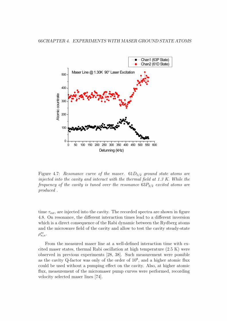
66CHAPTER 4. EXPERIMENTSWITHMASERGROUND STATE ATOMS
Figure 4.7: Resonance curve of the maser. 61D5/2 ground state atoms areinjected into the cavity and interact with the thermal field at 1.3 K. While thefrequency of the cavity is tuned over the resonance 63P3/2 excited atoms areproduced .
time τint, are injected into the cavity. The recorded spectra are shown in figure4.8. On resonance, the different interaction times lead to a different inversionwhich is a direct consequence of the Rabi dynamic between the Rydberg atomsand the microwave field of the cavity and allow to test the cavity steady-stateρssn,n.
From the measured maser line at a well-defined interaction time with ex-cited maser states, thermal Rabi oscillation at high temperature (2.5 K) wereobserved in previous experiments [28, 38]. Such measurement were possibleas the cavity Q-factor was only of the order of 108, and a higher atomic fluxcould be used without a pumping effect on the cavity. Also, at higher atomicflux, measurement of the micromaser pump curves were performed, recordingvelocity selected maser lines [74].
4.4. RABI OSCILLATIONS WITH A QUANTIZED THERMAL FIELD 67
(a)
(b) (c)
Figure 4.8: Resonance curve of the maser with velocity selection. 61D5/2
ground state atoms are injected into the cavity and interact with the thermalfield at 1.3 K, (a) τint = 94µs, (b) τint = 60µs, (c) τint = 50µs.
4.4 Rabi Oscillations with a Quantized Ther-
mal Field
As discussed in chapter 2, the interaction of a two-level atom with a singlemode of the cavity is described by the Jaynes-Cummings interaction. In thismodel, an atom in presence of a resonant quantum field exchanges periodicallyenergy (Rabi oscillations) and its population oscillates in a coherent way. Therealization of high Q cavity where the cavity decay constant γ is much smallerthan the Rabi frequency allows the realization of this coherent atom-field in-teraction. It is then possible to demonstrate the quantum nature of coherentlight with a collapse and revival of the Rabi oscillations observed using a spinecho measurement scheme [87]. Vacuum Rabi oscillations where an excitedstate atom |e〉 interacts with the vacuum field |0〉 of the cavity are also demon-
68CHAPTER 4. EXPERIMENTSWITHMASERGROUND STATE ATOMS
strated [29][30] in the micromaser experiment. However, inconsistencies withthe theoretical prediction of the vacuum Rabi oscillations remain. One possibleexplanation is attributed to higher field temperature. Until now, the cavitytemperature has been measured with a temperature sensor mounted on thecold finger, giving the temperature of the cavity wall. In fact, the cavity fieldcould be hotter due to outside radiation from hotter surfaces like the atomicoven or microwave waveguides which weakly couple into the cavity. Finally,the mean thermal photon number nth is together with the interaction time τintand the atomic rate R one of the free experimental parameter in the realiza-tion of the micromaser and it is therefore important to measure it accurately.To measure the cavity field temperature, 61D5/2 ground state atoms are usedas sensor.
At zero atomic flux, the cavity is in thermal equilibrium, and a blackbodyfield is present. At 1.3 K, the average number of thermal photons is 〈n〉th =0.85 and the cavity state reads:
ρth =∑n
〈n〉nth(1 + 〈n〉th)n+1
|n〉〈n| (4.17)
and the photon distribution in a thermal field is described by the Bose-Einsteindistribution:
ρn,n = 〈n|ρ|n〉
=〈n〉nth
(1 + 〈n〉th)n+1(4.18)
When a ground state atom enters the cavity, interaction with the black-body field starts, energy exchange occurs and the atomic population startsto oscillate. The atom absorbs a photon and is excited in the upper maserstate. The photon can be reemitted and the atom returns into the groundstate. Since the unperturbed field temperature of the cavity should be mea-sured, the average photon number should not be changed from one atom tothe other. The cavity reaches a thermal equilibrium on a timescale given byits decay time γ = 13 Hz and an atomic injection rate R much smaller than γis chosen. In the experiment, R < 1Hz. This ensures that each atom enteringthe cavity interacts with the field in thermal equilibrium and not a blackbodyfield modified under the interaction with the previous atom.
The experimental setup for the measurement of Rabi oscillations is equiva-lent to the one depicted in figure 4.4, used for the time-of-flight measurement.The laser pulse width is set to 3 µs (FWHM) giving a limitation to the inter-action time resolution. The time between two pulses is set to 100 ms which is

4.4. RABI OSCILLATIONS WITH A QUANTIZED THERMAL FIELD 69
larger than τf = 73ms the cavity decay time. Also, the laser intensity is chosenso that less that one atom per pulse is excited into the Rydberg state. Therecorded signal is averaged over 1000 events. For each velocity component, theatoms undergo different Rabi cycles. The probability to detect the atom inthe ground state is:
Pg =∑n=0
ρn,n cos2(√ngτ) (4.19)
0 10 20 30 40 50 60 70 80 90 100 110 120 130
0,0
0,2
0,4
0,6
0,8
1,0
Inversion
Interaction Time [µs]
Figure 4.9: Experimental realization of Rabi oscillations between 61D5/2 maserground state and the blackbody radiation of the cavity. The temperature of thecavity wall is 1.3K corresponding to 〈n〉th = 0.85 photon. The blue curve showsthe theoretical expectation for a Rabi oscillation at this field temperature. Thegreen and red curve show simulations at higher field temperature with 〈n〉th = 1and 〈n〉th = 1.37, respectively.
Figure 4.9 shows the realization of Rabi oscillation between ground stateatoms and the thermal field of the cavity. The observed quantity is the so-
70CHAPTER 4. EXPERIMENTSWITHMASERGROUND STATE ATOMS
called inversion giving a detection efficiency independent observation of thedynamics:
Inv =Pg − PePg + Pe
=∑n=0
ρn,n cos(2√ngτ) (4.20)
The resolution of the measured Rabi oscillations is comparable to the re-sults achieved by Rempe et al. [28], where the observed dynamics at highertemperature was extracted from maser-lines measurement.
The extracted coupling constant g/2π = 7.4±0.1 kHz, is in good agreementwith theoretically predicted values and with the previous measurement of ∼ 7kHz [26, 29, 30].
The extracted average thermal photon number is 〈n〉th = 1.13± 0.14. Thecavity wall temperature measured by a sillicium diode temperature sensor, is1.3 K and remained constant during the experiment. This corresponds to anaverage photon number of 〈n〉th = 0.85. The blue curve represent the realiza-tion of such oscillations. Mean photon numbers of 〈n〉th = 1 and 〈n〉th = 1.37correspond to field temperatures of 1.47 K and 1.56 K respectively. Therefore,it can be deduced, that the actual field temperature is slightly higher than thecavity wall temperature. This has to be taken into account when analyzingformer Rabi oscillations measurements.

Chapter 5
Optical Spectroscopy ofRydberg Atoms
In Chapter 4, the first cavity QED experiments with maser ground state atoms,the Rydberg 61D5/2 state, are shown. To perform these experiments, a newdiode laser system has been developed leading to the demonstration of a newpurely optical spectroscopy method of Rydberg atoms in a room-temperaturegas-cell. This new method is based on an electron shelving scheme and is thesubject of this Chapter. The excitation of Rydberg states is monitored by ob-serving the absorption of a laser locked on the strong D2 line. Applied to differ-ent excitations schemes, this method demonstrates a wide range of applicationsfor Rydberg atoms experiments. In particular, stabilization of a frequency dou-bled dye laser in the UV to one Rydberg transition is demonstrated.
Rydberg atoms with principal quantum numbers n >> 1 have exagger-ated atomic properties. The micromaser experiment takes advantage of thelarge dipole-dipole interactions that scales in n4 or the long radiative lifetimesthat scale in n3. In the last decade, Rydberg atoms start to play a majorrole for quantum information processes [88]. Taking advantage of the Rydbergatom properties, the implementation of quantum gates between neutral atomqbits was proposed a decade ago [89]. However, until very recently, in themost experiments the detection of the Rydberg atom was done in an indirectdestructive electronic scheme where Rydberg atoms are ionized first and theionizations products are detected electronically afterwards. This includes stateselective ionization in a static electrical field as the most common technique,since it combines high detection efficiency and Rydberg states discrimination(see chapter 3) [90]. Therefore, the development of a non-destructive detectionscheme of Rydberg atoms is of great interest.
71
72 CHAPTER 5. OPTICAL SPECTROSCOPY OF RYDBERG ATOMS
In this chapter, a new method of Doppler-free, purely optical detection oflaser excited Rb Rydberg atoms in a room-temperature gas cell is presented.The Rydberg atoms are excited from the ground state by the laser systems usedin the micromaser experiment, either in a single-excitation step with UV lightat 297 nm or in a two or three-step diode laser cascade setup. The detectionis performed as the absorption of the 780 nm diode laser on the strong RbD2 line is monitored in a scheme similar to the electron shelving. In the firstpart, the detection of weak transitions using the electron shelving techniquewill be introduced. Results of the non-destructive Rydberg spectroscopy of Rbatoms in a gas cell will be presented. Finally, the implementation of this newmethod in the laser stabilization scheme for the micromaser experiment willbe explained.
5.1 Weak Transition Detection by Electron Shel-
ving
Purely optical detection of high lying atomic Rydberg states has been a dif-ficult task for many years. This is mostly due to the small radial part of thedipole matrix element between the atomic ground state and the highly excitedRydberg states, leading to small absorption cross-sections and therefore poorabsorption or fluorescence signals. In early experiments on optical detection ofRydberg transitions with Ba atoms, the fluorescence of absorptions lines hasbeen observed in continuous spectra of picosecond laser pulses [91][92]. How-ever, the high temperatures of the glass cell needed to achieve a high atomicdensity does not allow any sub-Doppler spectroscopy. Doppler-free fluores-cence detection has been limited to low-lying Rydberg levels (n=7, 9 and 10)with Cs atoms [93].
Weak atomic transition have to be detected as they offer the highest fre-quency resolution. In atomic optical clocks experiments [17][94] or quan-tum information experiments based on trapped ions [18] the detection ofweak atomic transitions is performed using the quantum amplification of theelectron-shelving technique introduced by Dehmelt [19]. Considering a three-level atomic system in a V scheme. The transition |1〉 ↔ |2〉 is the so-calledstrong transition with τ2 the atomic lifetime of the state |2〉, while the tran-sition |1〉 ↔ |3〉 is the so-called weak transition with τ3 the atomic lifetimeof the state |3〉. The key of the detection scheme is the so-called quantumamplification which occurs when the detected signal is not the absorption orfluorescence caused by the transition itself but the fluorescence emitted onthe strong transition. In absence of the weak transition (for example whenthe laser is off-resonant), the atom undergoes many absorption-emission cy-
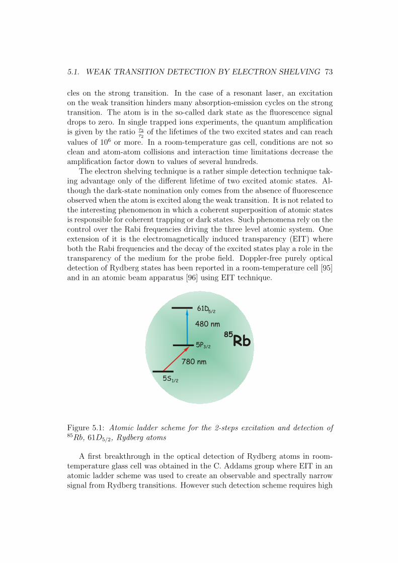
5.1. WEAK TRANSITION DETECTION BY ELECTRON SHELVING 73
cles on the strong transition. In the case of a resonant laser, an excitationon the weak transition hinders many absorption-emission cycles on the strongtransition. The atom is in the so-called dark state as the fluorescence signaldrops to zero. In single trapped ions experiments, the quantum amplificationis given by the ratio τ3
τ2of the lifetimes of the two excited states and can reach
values of 106 or more. In a room-temperature gas cell, conditions are not soclean and atom-atom collisions and interaction time limitations decrease theamplification factor down to values of several hundreds.
The electron shelving technique is a rather simple detection technique tak-ing advantage only of the different lifetime of two excited atomic states. Al-though the dark-state nomination only comes from the absence of fluorescenceobserved when the atom is excited along the weak transition. It is not related tothe interesting phenomenon in which a coherent superposition of atomic statesis responsible for coherent trapping or dark states. Such phenomena rely on thecontrol over the Rabi frequencies driving the three level atomic system. Oneextension of it is the electromagnetically induced transparency (EIT) whereboth the Rabi frequencies and the decay of the excited states play a role in thetransparency of the medium for the probe field. Doppler-free purely opticaldetection of Rydberg states has been reported in a room-temperature cell [95]and in an atomic beam apparatus [96] using EIT technique.
780 nm
480 nm
Rb85
61D 5/2
5P3/2
5S1/2
Figure 5.1: Atomic ladder scheme for the 2-steps excitation and detection of85Rb, 61D5/2, Rydberg atoms
A first breakthrough in the optical detection of Rydberg atoms in room-temperature glass cell was obtained in the C. Addams group where EIT in anatomic ladder scheme was used to create an observable and spectrally narrowsignal from Rydberg transitions. However such detection scheme requires high
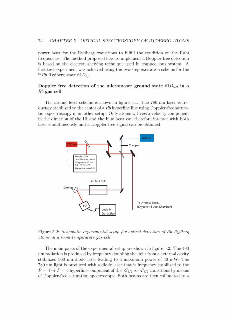
74 CHAPTER 5. OPTICAL SPECTROSCOPY OF RYDBERG ATOMS
power laser for the Rydberg transitions to fulfill the condition on the Rabifrequencies. The method proposed here to implement a Doppler-free detectionis based on the electron shelving technique used in trapped ions system. Afirst test experiment was achieved using the two-step excitation scheme for the85Rb Rydberg state 61D5/2.
Doppler free detection of the micromaser ground state 61D5/2 in aRb gas cell
The atomic-level scheme is shown in figure 5.1. The 780 nm laser is fre-quency stabilized to the center of a Rb hyperfine line using Doppler-free satura-tion spectroscopy in an other setup. Only atoms with zero-velocity componentin the direction of the IR and the blue laser can therefore interact with bothlaser simultaneously and a Doppler-free signal can be obtained.
780 nm
Doppler free
Stabilization to one
Component of the
5S 1/2 3P 3/2
Hyperfine manyfold
PD
Lock-in
Detection
480 nm
To Atomic Beam
(Cryostat & Aux.Chamber)
Rb Gas Cell
Chopper
Grating
Figure 5.2: Schematic experimental setup for optical detection of Rb Rydbergatoms in a room-temperature gas-cell
The main parts of the experimental setup are shown in figure 5.2. The 480nm radiation is produced by frequency doubling the light from a external cavitystabilized 960 nm diode laser leading to a maximum power of 40 mW. The780 nm light is produced with a diode laser that is frequency stabilized to theF = 3→ F = 4 hyperfine component of the 5S1/2 to 5P3/2 transitions by meansof Doppler-free saturation spectroscopy. Both beams are then collimated to a
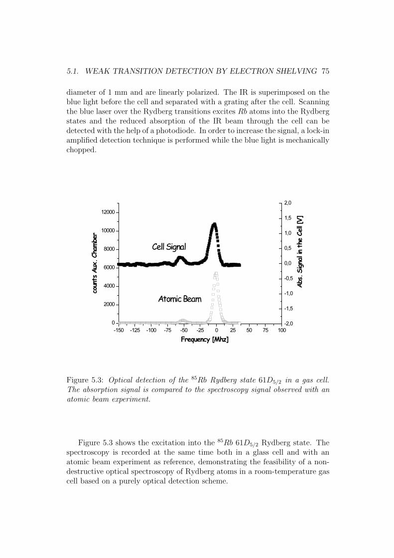
5.1. WEAK TRANSITION DETECTION BY ELECTRON SHELVING 75
diameter of 1 mm and are linearly polarized. The IR is superimposed on theblue light before the cell and separated with a grating after the cell. Scanningthe blue laser over the Rydberg transitions excites Rb atoms into the Rydbergstates and the reduced absorption of the IR beam through the cell can bedetected with the help of a photodiode. In order to increase the signal, a lock-inamplified detection technique is performed while the blue light is mechanicallychopped.
Figure 5.3: Optical detection of the 85Rb Rydberg state 61D5/2 in a gas cell.The absorption signal is compared to the spectroscopy signal observed with anatomic beam experiment.
Figure 5.3 shows the excitation into the 85Rb 61D5/2 Rydberg state. Thespectroscopy is recorded at the same time both in a glass cell and with anatomic beam experiment as reference, demonstrating the feasibility of a non-destructive optical spectroscopy of Rydberg atoms in a room-temperature gascell based on a purely optical detection scheme.

76 CHAPTER 5. OPTICAL SPECTROSCOPY OF RYDBERG ATOMS
5.2 Non-Destructive Spectroscopy of Rydberg
Atoms
Once a proof of principle experiment is realized in a two-step excitation scheme,the extension to other excitation schemes is discussed in this section. In addi-tion, it is shown, how optical pumping can be used to excite only one singlehyperfine level in the Rydberg hyperfine manyfold. As these hyperfine statesare separated by just a few kHz, they are usually not resolved spectroscopically.
Optical Spectroscopy with a 297 nm UV Laser
(a)
(b)
Figure 5.4: (a) Level atomic V scheme for the excitation and detection of 85Rb,63P3/2, Rydberg atoms; (b) schematic experimental setup for optical detectionof UV-Rydberg transitions in a room-temperature gas cell
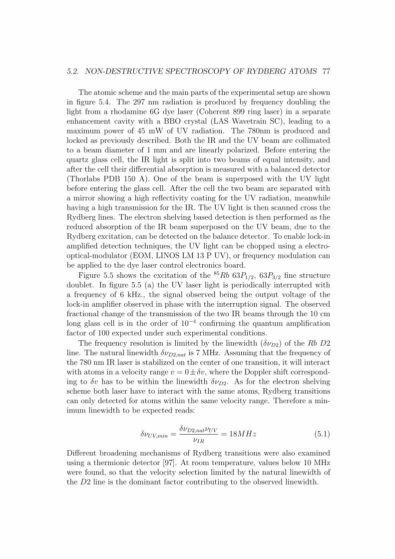
5.2. NON-DESTRUCTIVE SPECTROSCOPY OF RYDBERG ATOMS 77
The atomic scheme and the main parts of the experimental setup are shownin figure 5.4. The 297 nm radiation is produced by frequency doubling thelight from a rhodamine 6G dye laser (Coherent 899 ring laser) in a separateenhancement cavity with a BBO crystal (LAS Wavetrain SC), leading to amaximum power of 45 mW of UV radiation. The 780nm is produced andlocked as previously described. Both the IR and the UV beam are collimatedto a beam diameter of 1 mm and are linearly polarized. Before entering thequartz glass cell, the IR light is split into two beams of equal intensity, andafter the cell their differential absorption is measured with a balanced detector(Thorlabs PDB 150 A). One of the beam is superposed with the UV lightbefore entering the glass cell. After the cell the two beam are separated witha mirror showing a high reflectivity coating for the UV radiation, meanwhilehaving a high transmission for the IR. The UV light is then scanned cross theRydberg lines. The electron shelving based detection is then performed as thereduced absorption of the IR beam superposed on the UV beam, due to theRydberg excitation, can be detected on the balance detector. To enable lock-inamplified detection techniques, the UV light can be chopped using a electro-optical-modulator (EOM, LINOS LM 13 P UV), or frequency modulation canbe applied to the dye laser control electronics board.
Figure 5.5 shows the excitation of the 85Rb 63P1/2, 63P3/2 fine structuredoublet. In figure 5.5 (a) the UV laser light is periodically interrupted witha frequency of 6 kHz., the signal observed being the output voltage of thelock-in amplifier observed in phase with the interruption signal. The observedfractional change of the transmission of the two IR beams through the 10 cmlong glass cell is in the order of 10−4 confirming the quantum amplificationfactor of 100 expected under such experimental conditions.
The frequency resolution is limited by the linewidth (δνD2) of the Rb D2line. The natural linewidth δνD2,nat is 7 MHz. Assuming that the frequency ofthe 780 nm IR laser is stabilized on the center of one transition, it will interactwith atoms in a velocity range v = 0±δv, where the Doppler shift correspond-ing to δv has to be within the linewidth δνD2. As for the electron shelvingscheme both laser have to interact with the same atoms, Rydberg transitionscan only detected for atoms within the same velocity range. Therefore a min-imum linewidth to be expected reads:
δνUV,min =δνD2,natνUV
νIR= 18MHz (5.1)
Different broadening mechanisms of Rydberg transitions were also examinedusing a thermionic detector [97]. At room temperature, values below 10 MHzwere found, so that the velocity selection limited by the natural linewidth ofthe D2 line is the dominant factor contributing to the observed linewidth.
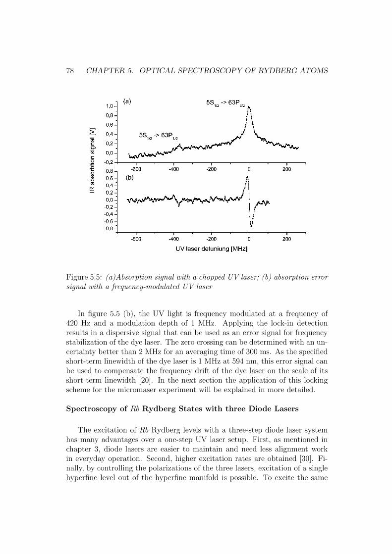
78 CHAPTER 5. OPTICAL SPECTROSCOPY OF RYDBERG ATOMS
Figure 5.5: (a)Absorption signal with a chopped UV laser; (b) absorption errorsignal with a frequency-modulated UV laser
In figure 5.5 (b), the UV light is frequency modulated at a frequency of420 Hz and a modulation depth of 1 MHz. Applying the lock-in detectionresults in a dispersive signal that can be used as an error signal for frequencystabilization of the dye laser. The zero crossing can be determined with an un-certainty better than 2 MHz for an averaging time of 300 ms. As the specifiedshort-term linewidth of the dye laser is 1 MHz at 594 nm, this error signal canbe used to compensate the frequency drift of the dye laser on the scale of itsshort-term linewidth [20]. In the next section the application of this lockingscheme for the micromaser experiment will be explained in more detailed.
Spectroscopy of Rb Rydberg States with three Diode Lasers
The excitation of Rb Rydberg levels with a three-step diode laser systemhas many advantages over a one-step UV laser setup. First, as mentioned inchapter 3, diode lasers are easier to maintain and need less alignment workin everyday operation. Second, higher excitation rates are obtained [30]. Fi-nally, by controlling the polarizations of the three lasers, excitation of a singlehyperfine level out of the hyperfine manifold is possible. To excite the same
5.2. NON-DESTRUCTIVE SPECTROSCOPY OF RYDBERG ATOMS 79
(a)
(b)
Figure 5.6: (a) Level scheme for the excitation of Rb Rydberg states in a threelaser cascade setup; (b) Laser setup for optical spectroscopy of Rb Rydbergatoms in a gas cell. The 780 and 776 nm lasers are frequency stabilized inseparate setups. These laser are counter propagating and their σ+, σ+ polar-ization is realized by two λ/4 plates. The 1256 nm laser can be applied fromboth sides.
63P3/2 state as with the UV laser, the dipole selection rules impose to use threeexcitation steps.
The experimental setup is shown in figure 5.6 (b). All three lasers aregrating-stabilized diode lasers (Toptica DL 100) equipped with standard diodelaser control electronics (Toptica DCC 100, DTC 100, SC 100). The firstlaser is resonant with the F = 3 → F = 4 hyperfine component of the D2line in 85Rb, and the laser is frequency-stabilized using Doppler-free saturationspectroscopy.
The second stage is resonant with the 5P3/2 → 5D5/2 transition at 775.8nm. As the lifetime of the 5D5/2 is 10 times longer as that of the 5P3/2 level, itsspectroscopic detection in a gas cell is already more challenging. Many groupsuse the 420 nm fluorescence emitted when the 6P levels, which are populatedfrom the 5D levels, decay back to the 5S ground state. Here, a different
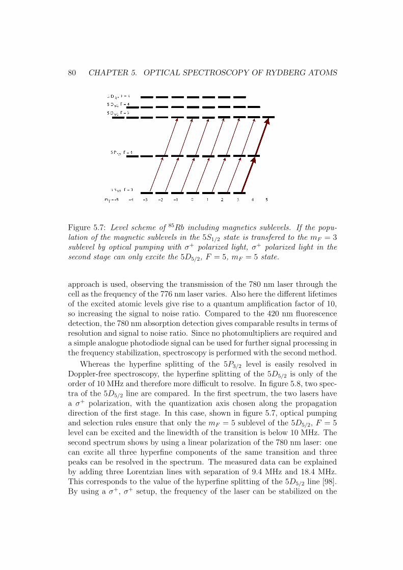
80 CHAPTER 5. OPTICAL SPECTROSCOPY OF RYDBERG ATOMS
Figure 5.7: Level scheme of 85Rb including magnetics sublevels. If the popu-lation of the magnetic sublevels in the 5S1/2 state is transfered to the mF = 3sublevel by optical pumping with σ+ polarized light, σ+ polarized light in thesecond stage can only excite the 5D5/2, F = 5, mF = 5 state.
approach is used, observing the transmission of the 780 nm laser through thecell as the frequency of the 776 nm laser varies. Also here the different lifetimesof the excited atomic levels give rise to a quantum amplification factor of 10,so increasing the signal to noise ratio. Compared to the 420 nm fluorescencedetection, the 780 nm absorption detection gives comparable results in terms ofresolution and signal to noise ratio. Since no photomultipliers are required anda simple analogue photodiode signal can be used for further signal processing inthe frequency stabilization, spectroscopy is performed with the second method.
Whereas the hyperfine splitting of the 5P3/2 level is easily resolved inDoppler-free spectroscopy, the hyperfine splitting of the 5D5/2 is only of theorder of 10 MHz and therefore more difficult to resolve. In figure 5.8, two spec-tra of the 5D5/2 line are compared. In the first spectrum, the two lasers havea σ+ polarization, with the quantization axis chosen along the propagationdirection of the first stage. In this case, shown in figure 5.7, optical pumpingand selection rules ensure that only the mF = 5 sublevel of the 5D5/2, F = 5level can be excited and the linewidth of the transition is below 10 MHz. Thesecond spectrum shows by using a linear polarization of the 780 nm laser: onecan excite all three hyperfine components of the same transition and threepeaks can be resolved in the spectrum. The measured data can be explainedby adding three Lorentzian lines with separation of 9.4 MHz and 18.4 MHz.This corresponds to the value of the hyperfine splitting of the 5D5/2 line [98].By using a σ+, σ+ setup, the frequency of the laser can be stabilized on the
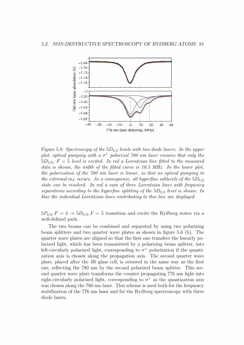
5.2. NON-DESTRUCTIVE SPECTROSCOPY OF RYDBERG ATOMS 81
Figure 5.8: Spectroscopy of the 5D5/2 levels with two diode lasers. In the upperplot, optical pumping with a σ+ polarized 780 nm laser ensures that only the5D5/2, F = 5 level is excited. In red a Lorentzian line fitted to the measureddata is shown, the width of the fitted curve is 10.5 MHz. In the lower plot,the polarization of the 780 nm laser is linear, so that no optical pumping tothe extremal mF occurs. As a consequence, all hyperfine sublevels of the 5D5/2
state can be resolved. In red a sum of three Lorentzian lines with frequencyseparations according to the hyperfine splitting of the 5D5/2 level is shown. Inblue the individual Lorentzian lines contributing to this line are displayed
5P3/2, F = 4 → 5D5/2, F = 5 transition and excite the Rydberg states via awell-defined path.
The two beams can be combined and separated by using two polarizingbeam splitters and two quarter wave plates as shown in figure 5.6 (b). Thequarter wave plates are aligned so that the first one transfers the linearly po-larized light, which has been transmitted by a polarizing beam splitter, intoleft-circularly polarized light, corresponding to σ+ polarization if the quanti-zation axis is chosen along the propagation axis. The second quarter waveplate, placed after the Rb glass cell, is oriented in the same way as the firstone, reflecting the 780 nm by the second polarized beam splitter. This sec-ond quarter wave plate transforms the counter propagating 776 nm light intoright-circularly polarized light, corresponding to σ+ as the quantization axiswas chosen along the 780 nm laser. This scheme is used both for the frequencystabilization of the 776 nm laser and for the Rydberg spectroscopy with threediode lasers.
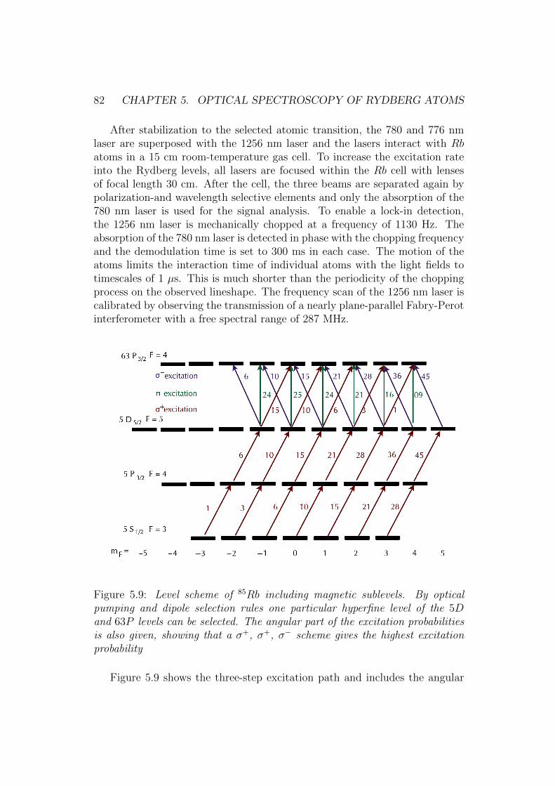
82 CHAPTER 5. OPTICAL SPECTROSCOPY OF RYDBERG ATOMS
After stabilization to the selected atomic transition, the 780 and 776 nmlaser are superposed with the 1256 nm laser and the lasers interact with Rbatoms in a 15 cm room-temperature gas cell. To increase the excitation rateinto the Rydberg levels, all lasers are focused within the Rb cell with lensesof focal length 30 cm. After the cell, the three beams are separated again bypolarization-and wavelength selective elements and only the absorption of the780 nm laser is used for the signal analysis. To enable a lock-in detection,the 1256 nm laser is mechanically chopped at a frequency of 1130 Hz. Theabsorption of the 780 nm laser is detected in phase with the chopping frequencyand the demodulation time is set to 300 ms in each case. The motion of theatoms limits the interaction time of individual atoms with the light fields totimescales of 1 µs. This is much shorter than the periodicity of the choppingprocess on the observed lineshape. The frequency scan of the 1256 nm laser iscalibrated by observing the transmission of a nearly plane-parallel Fabry-Perotinterferometer with a free spectral range of 287 MHz.
Figure 5.9: Level scheme of 85Rb including magnetic sublevels. By opticalpumping and dipole selection rules one particular hyperfine level of the 5Dand 63P levels can be selected. The angular part of the excitation probabilitiesis also given, showing that a σ+, σ+, σ− scheme gives the highest excitationprobability
Figure 5.9 shows the three-step excitation path and includes the angular
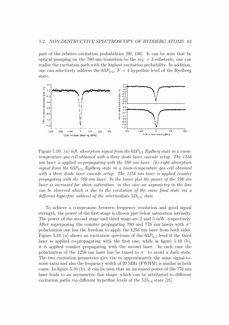
5.2. NON-DESTRUCTIVE SPECTROSCOPY OF RYDBERG ATOMS 83
part of the relative excitation probabilities [99, 100]. It can be seen that byoptical pumping on the 780 nm transition to the mF = 3 substrate, one canrealize the excitation path with the highest excitation probability. In addition,one can selectively address the 63P3/2, F = 4 hyperfine level of the Rydbergstate.
Figure 5.10: (a)-left, absorption signal from the 63P3/2 Rydberg state in a room-temperature gas cell obtained with a three diode laser cascade setup. The 1256nm laser is applied co-propagating with the 780 nm laser. (b)-right absorptionsignal from the 63P3/2 Rydberg state in a room-temperature gas cell obtainedwith a three diode laser cascade setup. The 1256 nm laser is applied counterpropagating with the 780 nm laser. In the lower plot the power of the 776 nmlaser is increased far above saturation. in this case an asymmetry in the linecan be observed which is due to the excitation of the same final state via adifferent hyperfine sublevel of the intermediate 5D5/2 state
To achieve a compromise between frequency resolution and good signalstrength, the power of the first stage is chosen just below saturation intensity.The power of the second stage and third stage are 2 and 5 mW, respectively.After superposing the counter propagating 780 and 776 nm lasers with σ+
polarization one has the freedom to apply the 1256 nm laser from both sides.Figure 5.10 (a) shows an excitation spectrum of the 63P3/2 level if the thirdlaser is applied co-propagating with the first one, while in figure 5.10 (b),it is applied counter propagating with the second laser. In each case thepolarization of the 1256 nm laser has be tuned to σ− to avoid a dark state.The two excitation geometries give rise to approximately the same signal-to-noise ratio and also the frequency width of 20 MHz (FWHM) is similar in bothcases. In figure 5.10 (b), it can be seen that an increased power of the 776 nmlaser leads to an asymmetric line shape, which can be attributed to differentexcitation paths via different hyperfine levels of the 5D5/2 state [21].

84 CHAPTER 5. OPTICAL SPECTROSCOPY OF RYDBERG ATOMS
In addition to the P levels, the Rydberg F levels can be reached with athree-step excitation as well. Figure 5.11 shows a spectrum of the 60F state,which is detuned 11.5 GHz below the 63P state. In this case linear polarizationhas been chosen for all three lasers and all lasers are co-propagating.
Figure 5.11: Excitation signal from the 60FRydberg state in a room-temperature gas cell obtained with a three diode laser cascade setup.
The quantum amplification effect, which has already been described above,is also responsible for the observation of the Rydberg transitions in a three-stepexcitation setup. As an excitation to the 5D state already hinders 10 absorp-tion and emission cycles on the D2 line, the quantum amplification for thethree-step excitation is expected to be reduced by the same factor if comparedwith the single-single step excitation in a V scheme. Nevertheless, the avail-able interaction time in the cell of about 1 µs in a focused laser beam leavesenough time for a quantum amplification effect of about 50, which explainsthe good signal-to noise ratio in the observed spectra.
5.3 Applications to the Micromaser Experi-
ment
In the previous section the optical spectroscopy of Rydberg atoms in a gascell is demonstrated. This method presents also the advantage that Rydbergtransition in a gas cell are highly immune to linear and quadratic DC-Starkshifts [95], giving these Rydberg lines an unexpectedly high frequency stability
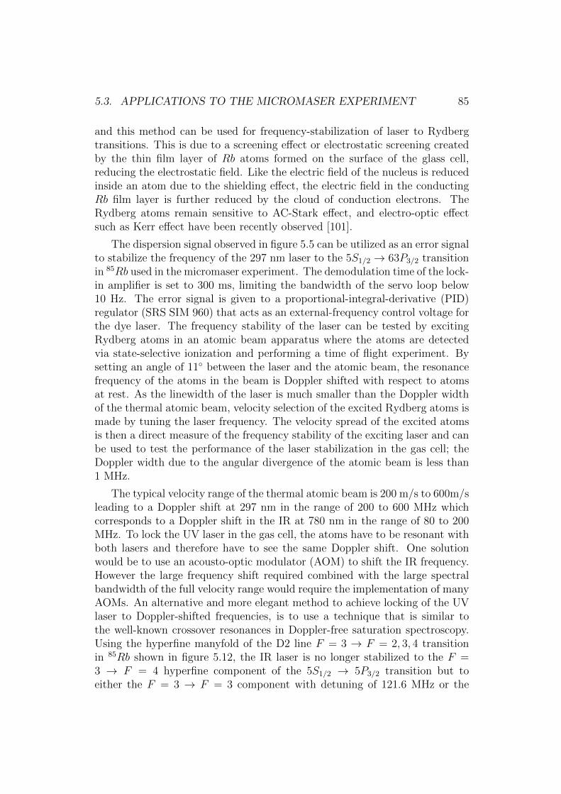
5.3. APPLICATIONS TO THE MICROMASER EXPERIMENT 85
and this method can be used for frequency-stabilization of laser to Rydbergtransitions. This is due to a screening effect or electrostatic screening createdby the thin film layer of Rb atoms formed on the surface of the glass cell,reducing the electrostatic field. Like the electric field of the nucleus is reducedinside an atom due to the shielding effect, the electric field in the conductingRb film layer is further reduced by the cloud of conduction electrons. TheRydberg atoms remain sensitive to AC-Stark effect, and electro-optic effectsuch as Kerr effect have been recently observed [101].
The dispersion signal observed in figure 5.5 can be utilized as an error signalto stabilize the frequency of the 297 nm laser to the 5S1/2 → 63P3/2 transitionin 85Rb used in the micromaser experiment. The demodulation time of the lock-in amplifier is set to 300 ms, limiting the bandwidth of the servo loop below10 Hz. The error signal is given to a proportional-integral-derivative (PID)regulator (SRS SIM 960) that acts as an external-frequency control voltage forthe dye laser. The frequency stability of the laser can be tested by excitingRydberg atoms in an atomic beam apparatus where the atoms are detectedvia state-selective ionization and performing a time of flight experiment. Bysetting an angle of 11 between the laser and the atomic beam, the resonancefrequency of the atoms in the beam is Doppler shifted with respect to atomsat rest. As the linewidth of the laser is much smaller than the Doppler widthof the thermal atomic beam, velocity selection of the excited Rydberg atoms ismade by tuning the laser frequency. The velocity spread of the excited atomsis then a direct measure of the frequency stability of the exciting laser and canbe used to test the performance of the laser stabilization in the gas cell; theDoppler width due to the angular divergence of the atomic beam is less than1 MHz.
The typical velocity range of the thermal atomic beam is 200 m/s to 600m/sleading to a Doppler shift at 297 nm in the range of 200 to 600 MHz whichcorresponds to a Doppler shift in the IR at 780 nm in the range of 80 to 200MHz. To lock the UV laser in the gas cell, the atoms have to be resonant withboth lasers and therefore have to see the same Doppler shift. One solutionwould be to use an acousto-optic modulator (AOM) to shift the IR frequency.However the large frequency shift required combined with the large spectralbandwidth of the full velocity range would require the implementation of manyAOMs. An alternative and more elegant method to achieve locking of the UVlaser to Doppler-shifted frequencies, is to use a technique that is similar tothe well-known crossover resonances in Doppler-free saturation spectroscopy.Using the hyperfine manyfold of the D2 line F = 3 → F = 2, 3, 4 transitionin 85Rb shown in figure 5.12, the IR laser is no longer stabilized to the F =3 → F = 4 hyperfine component of the 5S1/2 → 5P3/2 transition but toeither the F = 3 → F = 3 component with detuning of 121.6 MHz or the

86 CHAPTER 5. OPTICAL SPECTROSCOPY OF RYDBERG ATOMS
-400 -350 -300 -250 -200 -150 -100 -50 0 50 100 150 200
-1
0
1
2
3
4
155 MHz
121 MHz
92 MHz
60.5 MHz
F=3 -> F=2
F=3 -> F=3
F=3 -> F=4
Doppler-free absorbtion on 85
Rb (5S1/2
, F=3) to (5P3/2
, F=2, 3, 4)
su
btr
acte
d d
op
lerf
ree
ab
so
rbtio
n s
ign
al [V
]
780 nm laser detuning [MHz]
-1000 -800 -600 -400 -200 0 200 400
050
100150200250300
co
un
t ra
te
UV Laser Detuning [MHz]
-1000 -800 -600 -400 -200 0 200 400
-0,6-0,4-0,20,00,20,40,6
-1000 -800 -600 -400 -200 0 200 400
-0,6-0,4-0,20,00,20,40,6
ab
so
rptio
n in
ga
s c
ell
-1000 -800 -600 -400 -200 0 200 400
-0,6-0,4-0,20,00,20,40,6
-1000 -800 -600 -400 -200 0 200 400
-0,4-0,20,00,20,4
Figure 5.12: Left; the hyperfine manyfold of the D2 transition line in 85Rb.Right; (a) Doppler-shifted signal from an atomic beam under angular excita-tion; (b)-(e) shifted dispersive signal from a gas cell with a 780 nm laser lockedto (b) F = 3 → F = 4 resonance, (c) F = 3 → F = 2, 4 crossoverline, (d)F = 3→ F = 3 resonance, and (e) F = 3→ F = 2, 3 crossoverline
F = 3 → F = 2, 4 and F = 3 → F = 2, 3 crossoverlines with frequencydetuning of 92.5 MHz and 153.3 MHz, respectively. The F = 3 → F = 4 isnow resonant with atoms having a well-defined velocity and the UV Rydbergtransition is Doppler shifted by a frequency of:
∆νUV = ∆νIRνUVνIR
(5.2)
Figure 5.12 shows the Rydberg excitation signal in the gas cell for differentfrequencies of the IR laser and, for comparison, the spectrum obtained froman atomic beam under angular excitation. It is clearly seen that the Dopplershifted dispersive signal can be used to lock the UV laser on a frequency thatallows velocity-selective excitation in an atomic beam. With these lines, onesingle AOM can be enough to cover the Doppler shifts of the hole velocityspectrum of the atomic beam.
By making short UV excitation pulses of 5 µs duration with a mechanicalchopper and detecting the atoms 10 cm behind the excitation region, a time-of-flight spectrum can be recorded with the same method described in
5.3. APPLICATIONS TO THE MICROMASER EXPERIMENT 87
! "! #!! #"! $!! $"! %!! %"! &!! &"! "!!'"
!
"
#!
#"
$!
$"
%!
%"
()*+,-,.!"/01!
2340,56,673892,:"/01,;
<=>
?5@A2/
! "! #!! #"! $!! $"! %!! %"! &!! &"! "!!'"
!
"
#!
#"
$!
$"
%!
%"
&!
&"
"!
""
(!
("
)!
*+,-./.(0"!"123!
456
789:;1
;<=2.8>.>?<@A;.B"123.C
Figure 5.13: Time-of-flight spreding of Rydberg atoms after velocity selectiveexcitation in an atomic beam; (a) the IR laser is locked on the F = 3→ F =2, 3 crossoverline with UV laser detuning of 402 MHz ; (b) the IR laser islocked on the F = 3→ F = 3 resonance with UV laser detuning of 319 MHz
Chapter 4 to measure Rabi oscillations. Figure 5.13 shows the distribution ofarrival times for UV laser detuning of 402 MHz (left) and 319 MHz (right).From the width of this distribution (6.5-8 µS), the laser frequency stays withina frequency window of 2 MHz in the UV over recording times of severalhours. As this number coincides with the short-term frequency stability ofthe frequency-doubled dye laser, the long-term frequency stabilization of thelaser on the level of its short-time linewidth is demonstrated. The results com-pare also very well with the results obtained by stabilizing the laser frequencyto the signal obtained from state-selective ionization in an atomic beam, withthe advantage of a much simpler setup, involving no vacuum chamber and nocryogenic cooling.

88 CHAPTER 5. OPTICAL SPECTROSCOPY OF RYDBERG ATOMS
Chapter 6
Quantum Trajectories
Parallel to the realization of cavity QED experiments with ground state atomsand the development of a new spectroscopy method of Rydberg atoms in a gascell, a numerical and theoretical work supporting the ongoing experiments hasbeen achieved. The time dependence of the micromaser field can not be solvedanalytically and therefore numerical treatment has to be performed. For thestudy of the micromaser linewidth and the measurement of the phase diffu-sion, a numerical simulation method has been developed using the QuantumTrajectory Method. Finally, the realization of quantum Ramsey interferencesin a toroidal cavity developed for the realization of Quantum Non Demolition(QND) measurements is theoretically demonstrated.
In Chapter 2, a general theoretical introduction about the one-atom maserhas be done and the steady-state of the micromaser field has been analyticallycalculated. However, there are no analytical solutions for the time dependenceof the field density matrix ρ, except in the particular case of trapping states atzero temperature. In order to go beyond the approximations of an analyticaltreatment of the time evolution of the cavity field, one has to take recourseto numerical methods. The micromaser is ideally suited for treatments by nu-merical simulation (Monte Carlo) methods. The random arrival time of eachatom can be easily modeled, and the calculation of the field change due tothe passage of each atom is straightforward as the effect of the cavity decaybetween the passage of two atoms can also be readily calculated [102][103].By carrying out this procedure for a sequence of atoms during a time interval(0, t), repeating it and averaging it, it is possible to reconstruct the time evo-lution of the cavity field ρ(t) for a given ρ(0), or the time dependence of themean value of the cavity field variables [35]. Therefore there are many simi-larities between the methods used to analyze the micromaser features and thequantum trajectory method (QTM) used in quantum optics in the treatment
89
90 CHAPTER 6. QUANTUM TRAJECTORIES
of Markovian master equation [104][105][106]. Rather than solving the masterequation for a density operator itself, the method involves the construction ofan ensemble of states statistically equivalent to the density operator solution.These states evolve stochastically by non-unitary operations for a certain timeinterval interrupted at random by discontinuous changes of state, e.g ”Quan-tum Jumps”. For example an atom entering the cavity in the upper stateundergoing a transition to the lower maser state as it emits a photon, or, inthe case of cavity decay as for the micromaser, the loss of a photon from thecavity to the environment.
However the correspondence between the master equation and the ensembleof trajectories is not unique as the kinds of quantum jump is not unique. If thedifferent ensembles that can be generated, all correspond to the same densityoperator, they can represent the master equation. In the case each state ofthe ensemble is pure and remains pure through the time evolution governedby a non-linear stochastic Schrodinger equation, only N components fromthe state vector are needed, compared to the N2 components of the densityoperator showing an advantage for large N as a large number of simulationsare necessary to obtain statistically reliable averages.
Nevertheless QTM is more than a calculation tool and is connected toquantum measurement theory. The master equation describes the irreversibledynamics of a dissipative system coupled to a reservoir. In the case of themicromaser, the atoms leaving the cavity can be understood as decay productsof the cavity. Therefore the detection of these atoms represents from a quantummeasurement perspective the acquisition of information by the observer, andwith each detection the cavity field will be projected into a new state, e.gundergoing a quantum jump, conditioned on the detection results. An explicitconnection is established between a quantum trajectory and a macroscopicrecord of detection and a quantum trajectory analysis of the master equationcan be built around the chosen detection scheme.
The essential elements of a quantum trajectory are explicitly built into themicromaser by the presence of the atomic beam. The cavity field evolution,e.g decay, is interrupted by a quantum jump due to the presence of an atomat a random time, representing one unravelling of the micromaser dynamics.
In the following section, the quantum formalism applied to the micromaserand its application for numerical simulations will be presented. The particularcase of phase diffusion in the micromaser and quantum Ramsey interferencesin a toroidal cavity will be discussed.
6.1. QTM APPLIED TO THE MICROMASER 91
6.1 QTM applied to the Micromaser
The quantum trajectory formalism will be outlined here in reference to themaster equation (2.57) introduced in Chapter 2. The Markovian master equa-tion for Poissonian pumping can be written as:
∂ρ
∂t= R(A− 1 + L)ρ (6.1)
with:
Aρ = cos(gτ√a†a+ 1)ρ(t0) cos(gτ
√a†a+ 1)+
a†sin(gτ
√a†a+ 1)√
a†a+ 1ρ(to)
sin(gτ√a†a+ 1)√
a†a+ 1a (6.2)
Equation (6.1) can be re-expressed in terms of a set of operators Ci, i =−1, 0, 1, 2 with:
C−1 =√γ(nth + 1)a (6.3)
which corresponds to the loss of a photon from the cavity field the the reservoir.The operator
C1 =√Ra† sin(gτ
√a†a+ 1)√
a†a+ 1(6.4)
is associated with the gain of a photon to the cavity from an atom passingthrough the cavity while,
C0 =√R cos(gτ
√a†a+ 1) (6.5)
corresponds to an atom in the excited state passing through the cavity withoutgiving a photon.Finally,
C2 =√γntha
† (6.6)
is associated to the gain of a photon from the reservoir.
With equation (2.49) expressing L and using:
Rρ =1
2(C†1C1 + C†0C0)ρ+
1
2ρ(C†1C1 + C†0C0) (6.7)
one can rewrite equation (6.1) in the form:
∂ρ
∂t=
2∑i=−1
[CiρC†i −
1
2(C†iCiρ+ ρC†iCi)] (6.8)
92 CHAPTER 6. QUANTUM TRAJECTORIES
The termsCiρC
†i = Jiρ (6.9)
can be associated with the system undergoing discrete jumps of type Ci asρ→ CiρC
†i with for exemple a gain of one photon in the cavity if the jump is
of type J1 or a loss of one photon for a J−1 operation. The operators Ji canthen be linearly combined to form a new operator J :
J ρ =∑i
CiρC†i =
∑i
Jiρ (6.10)
Now replacing L by L − J + J and using the identity:
e(A+ηB)t = eAt+∞∑n=1
ηn∫ t
0
dtn
∫ tn
0
dtn−1 · · ·∫ t2
0
dt1eA(t−tn)BeA(tn−tn−1)B · · ·BeAt1
(6.11)the solution for the time evolution of the cavity field reads:
ρ(t) = ρ(0)c (t)P (0)(t) +
∞∑n=1
∑i1
· · ·∑in
∫ t
0
dtn
∫ tn
0
dtn−1 · · ·∫ t2
0
dt1
× ρ(n)c (t; i1, t1, · · · , in, tn) (6.12)
× P (n)(i1, t1, · · · , in, tn; [0, t])
with:
ρ(0)c (t) =
e(L−J )t
Tr[e(L−J )tρ(0)]
P (0)(t) = Tr[e(L−J )tρ(0)] (6.13)
and
ρ(n)c (t;i1, t1, · · · , in, tn)
=e(L−J )(t−tn)Jine(L−J )(tn−tn−1)Jin−1 · · · Ji1e(L−J )(t1)ρ(0)
Tr[e(L−J )(t−tn)Jine(L−J )(tn−tn−1)Jin−1 · · · Ji1e(L−J )(t1)ρ(0)](6.14)
P (n)(i1, t1, · · · , in, tn; [0, t])
= Tr[e(L−J )(t−tn)Jine(L−J )(tn−tn−1)Jin−1 · · · Ji1e(L−J )(t1)ρ(0)]
6.1. QTM APPLIED TO THE MICROMASER 93
P (n) = 0, 1, 2, · · · , n can be interpreted as the probability that an event ofthe type in occurs in the time interval [tn, tn + dtn], P (0) being the probabilitythat no events happens in the time interval [0, t], e.g no atoms passing throughthe cavity during this time interval and no interaction between the cavity fieldand the environment. ρ(n)c(t;i1,t1n,tn) can be interpreted as the conditioned stateof the cavity at the time t. The conditioning is on n jumps of type i1, · · · , ininduced by the jump operators Ji, i = −1, 0, 1, 2 at the times t1, . . . , tn, whilethe system evolution is governed by the non-unitary operator e(L−J )t betweentwo jumps and given that the cavity is initially prepared in the state ρ(0).
The numerical implementation of the QTM is then realized by propagatingthe conditioned state through infinitesimal time steps, asking at the end ofeach step whether or not a jump has occurred and of which type it was [106].However a more efficient procedure is particularly suited for the micromaser.The principle is to evaluate after each jump, the time of occurrence of the nextjump. In other word, the conditioned state ρ(n)c(tn;i1,t1···in,tn) at the time tn willpropagate under the action of the non-unitary operators e(L−J )t until t = tn+1,the time of the next jump. tn+1 can be generated numerically by evaluatingthe probability that a jump of any kind occurs in the time interval [t(n), t(n+1)].[105] shows that the probability can be evaluated in terms of a new randomvariable r defined by:
r(t) = Tr[e(L−J )(t−tn)ρ(n)c (t; i1, t1 · · · , in, tn)] (6.15)
where r can be shown to be uniformly distributed on [0, 1]. Therefore, it ispossible to simulate the time of the (n + 1)th jump by choosing a randomnumber rn+1 from the distribution [0, 1] and calculating the time tn+1 of thenext jump by the condition:
rn+1 = Tr[e(L−J )(tn+1−tn)ρ(n)c (tn; i1, t1 · · · , in, tn)] (6.16)
The remaining steps in the simulation are standards: the probability that ajump of type Ji occurs is given by:
Pi =Tr[Jiρ
(n)c (tn; i1, t1 · · · , in, tn)]
Tr[J ρ(n)c (tn; i1, t1 · · · , in, tn)]
(6.17)
and then the new conditioned state reads:
ρ(n+1)c (tn+1; i1, t1 · · · , in+1, tn+1) =
Jiρ(n)c (tn; i1, t1 · · · , in, tn)
Tr[J ρ(n)c (tn; i1, t1 · · · , in, tn)]
(6.18)
This state is then propagated till the next jump in an iterative way, usingthe procedure defined in (6.14) and (6.15) with new random number r and so

94 CHAPTER 6. QUANTUM TRAJECTORIES
until the trajectory completes the time of interest. Repeating the process withthe same initial state ρ(0) will generate a new trajectory. Averaging over alltrajectories allows the reconstruction of the state density operator ρ(t).
As previously mentioned, the operator J can be arbitrarly constructedfrom a linear combination from the different jump operators Ji. One possiblechoice would be to consider a jump of the cavity occurs only in the presence ofan atom and consider the interaction of the cavity field and the environmentas part of the evolution between two jumps. In this case:
J ρ = (J0 + J1)ρ
= cos(gτ√a†a+ 1)ρ cos(gτ
√a†a+ 1)+ (6.19)
a†sin(gτ
√a†a+ 1)√
a†a+ 1ρ
sin(gτ√a†a+ 1)√
a†a+ 1a
From the simulation procedure (6.14)− (6.16) the time of the (n+ 1)th jumpis given by:
rn+1 = e−R(tn+1−tn) (6.20)
which is the arrival time of the next atoms arriving in the cavity. This is onlydetermined by the statistical properties of the atomic beam and not by thedynamics of the system.
The simulation algorithm provided from this approach allows the simula-tion of the time-dependent density operator ρ(t) of the cavity field. Howeverin this case the individual quantum trajectories will produce mixed states ingeneral, even if the cavity is in an initial pure state. Therefore, the problem canbe simplified if only pure state conditioned operators need to be considered.If:
J = J−1 + J0 + J1 + J2 (6.21)
Then,
(L − J )ρ = −1
2γ(nth + 1)(a†aρ+ ρa†a)− 1
2γnth(a
†aρ+ ρa†a)−Rρ (6.22)
The operators Ji and (L − J ) have the properties of mapping pure statesinto pure states, leading to a quantum trajectory simulation in term of stochas-tically evolving pure states. In this case one can consider any change of thecavity as a jump operation as the state of the cavity remains unchanged be-tween two jumps.
For a conditioned state |m〉 after the jump at a time tn, the waiting timefor the next jump can be evaluated from (6.14):
tn+1 − tn =−R−1log(rn+1)
1 +R[(nth + 1)m+ nth(m+ 1)](6.23)
6.1. QTM APPLIED TO THE MICROMASER 95
while from (6.15) the probability that the next jump is of type i at tn+1 isgiven by:
p−1 =R(nth + 1)m
1 +R[(nth + 1)m+ nth(m+ 1)]|m〉 → |m− 1〉 (6.24)
p0 =cos2(g
√m+ 1τ)
1 +R[(nth + 1)m+ nth(m+ 1)]|m〉 → |m〉 (6.25)
p1 =sin2(g
√m+ 1τ)
1 +R[(nth + 1)m+ nth(m+ 1)]|m〉 → |m+ 1〉 (6.26)
and
p2 =Rnth(m+ 1)
1 +R[(nth + 1)m+ nth(m+ 1)]|m〉 → |m+ 1〉 (6.27)
P 0 does not involve any change of the cavity field but has to be taken intoaccount as it represents the case of an atom in the upper maser state passingtrough the cavity without letting a photon inside. As the detection schemeis based on the discrimination of the states of the atoms emerging from thecavity, it is also important to take this operation in consideration as one wantsto connect the quantum trajectory formalism with the theory of continuousmeasurement on an atomic beam [107].
Finally, as the cavity is initially in a thermal state at a finite temperatureT , the cavity density operator can be represented in the photon number basiswith its matrix element given by:
ρn,n(0) =nnth
(1 + nth)n+1(6.28)
The experimental conditions can therefore easily be implemented in thesimulation as one has access to all experimental free parameters (interactiontime, atomic pumping rate, and cavity temperature e.g initial thermal state ofthe cavity).
However, given the large number of trajectories (over 100 000) required toobtain significant results for the steady-state of the micromaser, it is undoubt-edly the case that using numerical simulations does not provide any advantageover a direct analytical treatment of the master equation. On the other handthe intimate connection between Quantum Trajectory Measurements and con-tinuous measurements also enables a different perspective on the applicationof the method to the micromaser, for example in the context of testing groundfor the quantum theory of continuous feedback [108, 109] or in the study ofcollective effects in the trapping state regime [110].
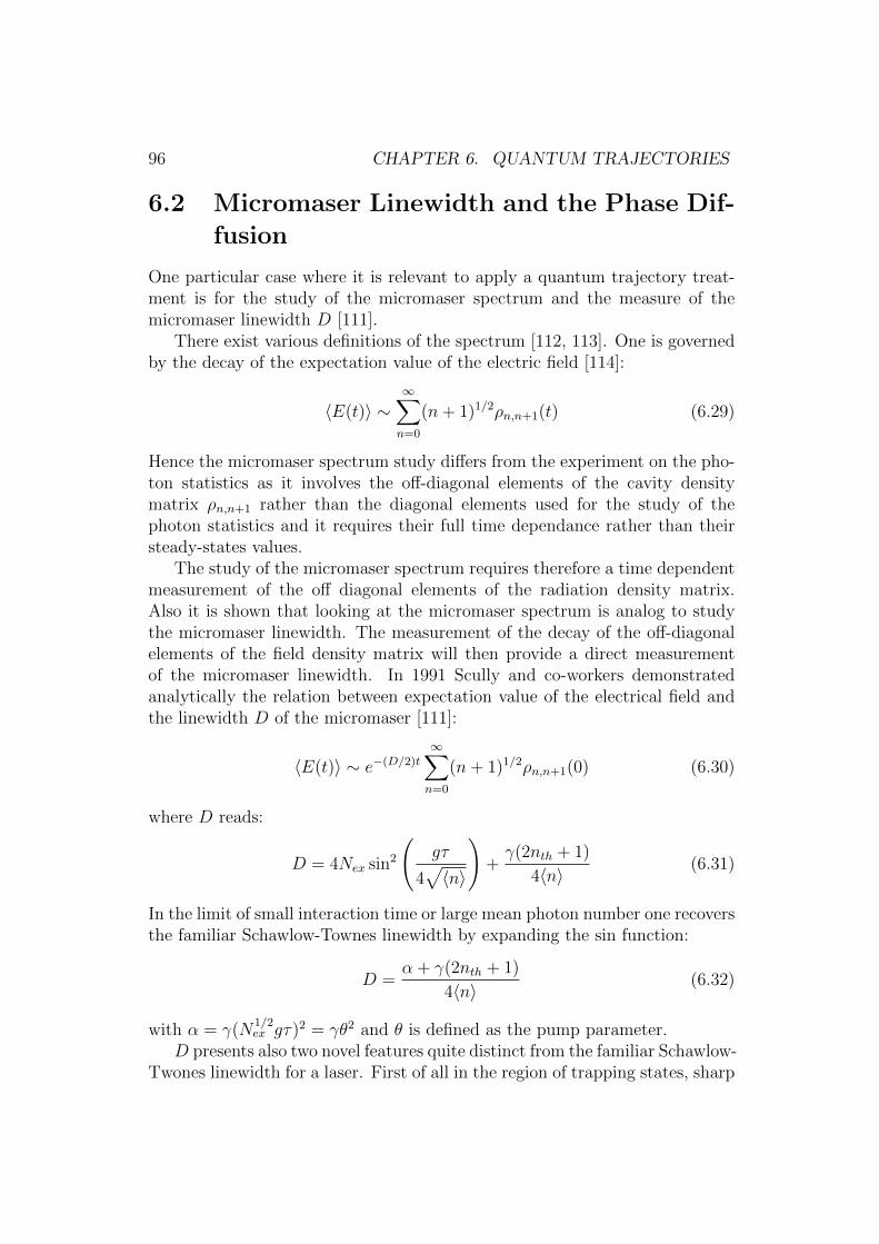
96 CHAPTER 6. QUANTUM TRAJECTORIES
6.2 Micromaser Linewidth and the Phase Dif-
fusion
One particular case where it is relevant to apply a quantum trajectory treat-ment is for the study of the micromaser spectrum and the measure of themicromaser linewidth D [111].
There exist various definitions of the spectrum [112, 113]. One is governedby the decay of the expectation value of the electric field [114]:
〈E(t)〉 ∼∞∑n=0
(n+ 1)1/2ρn,n+1(t) (6.29)
Hence the micromaser spectrum study differs from the experiment on the pho-ton statistics as it involves the off-diagonal elements of the cavity densitymatrix ρn,n+1 rather than the diagonal elements used for the study of thephoton statistics and it requires their full time dependance rather than theirsteady-states values.
The study of the micromaser spectrum requires therefore a time dependentmeasurement of the off diagonal elements of the radiation density matrix.Also it is shown that looking at the micromaser spectrum is analog to studythe micromaser linewidth. The measurement of the decay of the off-diagonalelements of the field density matrix will then provide a direct measurementof the micromaser linewidth. In 1991 Scully and co-workers demonstratedanalytically the relation between expectation value of the electrical field andthe linewidth D of the micromaser [111]:
〈E(t)〉 ∼ e−(D/2)t
∞∑n=0
(n+ 1)1/2ρn,n+1(0) (6.30)
where D reads:
D = 4Nex sin2
(gτ
4√〈n〉
)+γ(2nth + 1)
4〈n〉(6.31)
In the limit of small interaction time or large mean photon number one recoversthe familiar Schawlow-Townes linewidth by expanding the sin function:
D =α + γ(2nth + 1)
4〈n〉(6.32)
with α = γ(N1/2ex gτ)2 = γθ2 and θ is defined as the pump parameter.
D presents also two novel features quite distinct from the familiar Schawlow-Twones linewidth for a laser. First of all in the region of trapping states, sharp
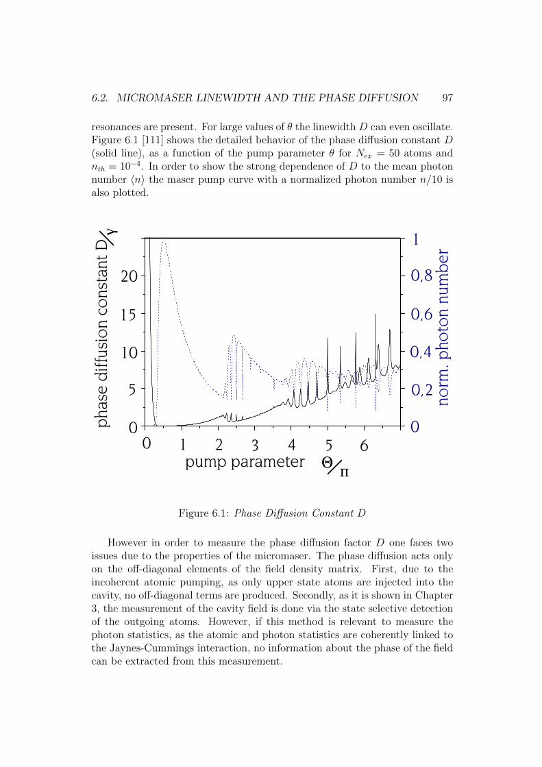
6.2. MICROMASER LINEWIDTH AND THE PHASE DIFFUSION 97
resonances are present. For large values of θ the linewidth D can even oscillate.Figure 6.1 [111] shows the detailed behavior of the phase diffusion constant D(solid line), as a function of the pump parameter θ for Nex = 50 atoms andnth = 10−4. In order to show the strong dependence of D to the mean photonnumber 〈n〉 the maser pump curve with a normalized photon number n/10 isalso plotted.
pump parameter Up
0 2 4 61 3 5
phase diffusion constant Dg
0
5
10
15
20
norm
. photon number
0
1
0,2
0,4
0,6
0,8
Figure 6.1: Phase Diffusion Constant D
However in order to measure the phase diffusion factor D one faces twoissues due to the properties of the micromaser. The phase diffusion acts onlyon the off-diagonal elements of the field density matrix. First, due to theincoherent atomic pumping, as only upper state atoms are injected into thecavity, no off-diagonal terms are produced. Secondly, as it is shown in Chapter3, the measurement of the cavity field is done via the state selective detectionof the outgoing atoms. However, if this method is relevant to measure thephoton statistics, as the atomic and photon statistics are coherently linked tothe Jaynes-Cummings interaction, no information about the phase of the fieldcan be extracted from this measurement.
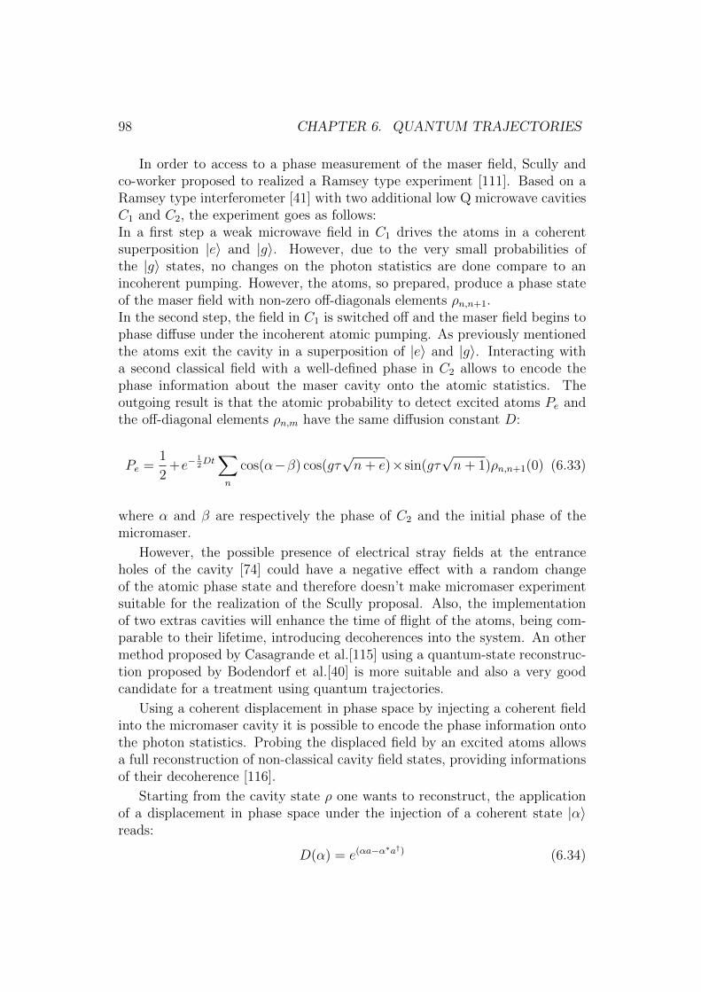
98 CHAPTER 6. QUANTUM TRAJECTORIES
In order to access to a phase measurement of the maser field, Scully andco-worker proposed to realized a Ramsey type experiment [111]. Based on aRamsey type interferometer [41] with two additional low Q microwave cavitiesC1 and C2, the experiment goes as follows:In a first step a weak microwave field in C1 drives the atoms in a coherentsuperposition |e〉 and |g〉. However, due to the very small probabilities ofthe |g〉 states, no changes on the photon statistics are done compare to anincoherent pumping. However, the atoms, so prepared, produce a phase stateof the maser field with non-zero off-diagonals elements ρn,n+1.In the second step, the field in C1 is switched off and the maser field begins tophase diffuse under the incoherent atomic pumping. As previously mentionedthe atoms exit the cavity in a superposition of |e〉 and |g〉. Interacting witha second classical field with a well-defined phase in C2 allows to encode thephase information about the maser cavity onto the atomic statistics. Theoutgoing result is that the atomic probability to detect excited atoms Pe andthe off-diagonal elements ρn,m have the same diffusion constant D:
Pe =1
2+e−
12Dt∑n
cos(α−β) cos(gτ√n+ e)×sin(gτ
√n+ 1)ρn,n+1(0) (6.33)
where α and β are respectively the phase of C2 and the initial phase of themicromaser.
However, the possible presence of electrical stray fields at the entranceholes of the cavity [74] could have a negative effect with a random changeof the atomic phase state and therefore doesn’t make micromaser experimentsuitable for the realization of the Scully proposal. Also, the implementationof two extras cavities will enhance the time of flight of the atoms, being com-parable to their lifetime, introducing decoherences into the system. An othermethod proposed by Casagrande et al.[115] using a quantum-state reconstruc-tion proposed by Bodendorf et al.[40] is more suitable and also a very goodcandidate for a treatment using quantum trajectories.
Using a coherent displacement in phase space by injecting a coherent fieldinto the micromaser cavity it is possible to encode the phase information ontothe photon statistics. Probing the displaced field by an excited atoms allowsa full reconstruction of non-classical cavity field states, providing informationsof their decoherence [116].
Starting from the cavity state ρ one wants to reconstruct, the applicationof a displacement in phase space under the injection of a coherent state |α〉reads:
D(α) = e(αa−α∗a†) (6.34)
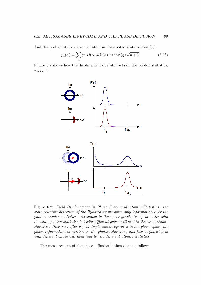
6.2. MICROMASER LINEWIDTH AND THE PHASE DIFFUSION 99
And the probability to detect an atom in the excited state is then [86]:
pe(α) =∑n
〈n|D(α)ρD†(α)|n〉 cos2(gτ√n+ 1) (6.35)
Figure 6.2 shows how the displacement operator acts on the photon statistics,e.g ρn,n.
Figure 6.2: Field Displacement in Phase Space and Atomic Statistics: thestate selective detection of the Rydberg atoms gives only information over thephoton number statistics. As shown in the upper graph, two field states withthe same photon statistics but with different phase will lead to the same atomicstatistics. However, after a field displacement operated in the phase space, thephase information is written on the photon statistics, and two displaced fieldwith different phase will then lead to two different atomic statistics.
The measurement of the phase diffusion is then done as follow:
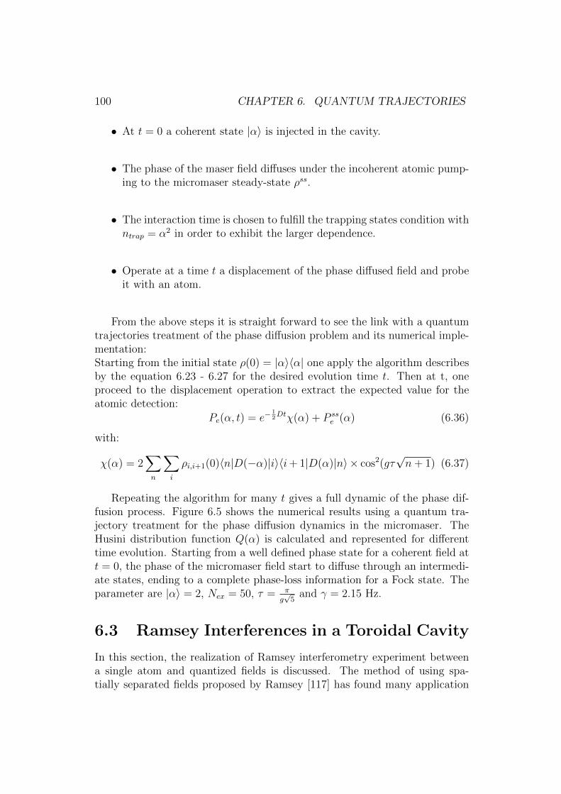
100 CHAPTER 6. QUANTUM TRAJECTORIES
• At t = 0 a coherent state |α〉 is injected in the cavity.
• The phase of the maser field diffuses under the incoherent atomic pump-ing to the micromaser steady-state ρss.
• The interaction time is chosen to fulfill the trapping states condition withntrap = α2 in order to exhibit the larger dependence.
• Operate at a time t a displacement of the phase diffused field and probeit with an atom.
From the above steps it is straight forward to see the link with a quantumtrajectories treatment of the phase diffusion problem and its numerical imple-mentation:Starting from the initial state ρ(0) = |α〉〈α| one apply the algorithm describesby the equation 6.23 - 6.27 for the desired evolution time t. Then at t, oneproceed to the displacement operation to extract the expected value for theatomic detection:
Pe(α, t) = e−12Dtχ(α) + P ss
e (α) (6.36)
with:
χ(α) = 2∑n
∑i
ρi,i+1(0)〈n|D(−α)|i〉〈i+ 1|D(α)|n〉 × cos2(gτ√n+ 1) (6.37)
Repeating the algorithm for many t gives a full dynamic of the phase dif-fusion process. Figure 6.5 shows the numerical results using a quantum tra-jectory treatment for the phase diffusion dynamics in the micromaser. TheHusini distribution function Q(α) is calculated and represented for differenttime evolution. Starting from a well defined phase state for a coherent field att = 0, the phase of the micromaser field start to diffuse through an intermedi-ate states, ending to a complete phase-loss information for a Fock state. Theparameter are |α〉 = 2, Nex = 50, τ = π
g√
5and γ = 2.15 Hz.
6.3 Ramsey Interferences in a Toroidal Cavity
In this section, the realization of Ramsey interferometry experiment betweena single atom and quantized fields is discussed. The method of using spa-tially separated fields proposed by Ramsey [117] has found many application
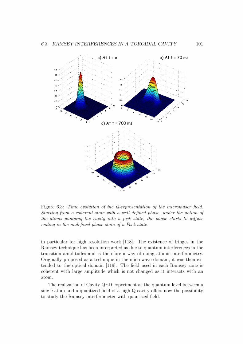
6.3. RAMSEY INTERFERENCES IN A TOROIDAL CAVITY 101
a) At t = o b) At t = 70 ms
c) At t = 700 ms
Figure 6.3: Time evolution of the Q-representation of the micromaser field.Starting from a coherent state with a well defined phase, under the action ofthe atoms pumping the cavity into a fock state, the phase starts to diffuseending in the undefined phase state of a Fock state.
in particular for high resolution work [118]. The existence of fringes in theRamsey technique has been interpreted as due to quantum interferences in thetransition amplitudes and is therefore a way of doing atomic interferometry.Originally proposed as a technique in the microwave domain, it was then ex-tended to the optical domain [119]. The field used in each Ramsey zone iscoherent with large amplitude which is not changed as it interacts with anatom.
The realization of Cavity QED experiment at the quantum level between asingle atom and a quantized field of a high Q cavity offers now the possibilityto study the Ramsey interferometer with quantized field.
102 CHAPTER 6. QUANTUM TRAJECTORIES
A two-level atom interacts for a well defined time τ with each cavity sepa-rate by a free evolution during the time of flight between the two cavities. Asfor the micromaser the atoms is then detected after the interaction with thesecond cavity. The two cavities have the same frequency ωF , as the two atomiclevels |e〉 and |g〉 have a frequency separation ωA. Using the Jaynes-Cummingsinteraction outlined in Chapter 2, the interaction between the atom and thecavity reads:
HAF = ~gi(a†σei∆t + aσ†e−i(∆)t) (6.38)
with the detuning ∆ = ωF − ωA, and gi are the atom-field coupling con-stant for the ith cavity. The cavity fields are initially in an arbitrary state∑
n,mPn,m|n,m〉 and the atom is prepared in the excited state |e〉.After the first interaction the wave function of the Atom-Field system reads:
ΨA−F (τ) =e−i∆τ∑n,m
Pn,m[cos(λn,1τ) +i∆
λn,1sin(λn,1τ)]|e, n,m〉
− iei∆τ∑n,m
Pn−1,mg1
√n+ 1
λn,1sin(λn,1τ)|g, n,m〉 (6.39)
with λn,1 =√
(∆2
)2 + g21(n+ 1) the generalized Rabi frequency for the first
cavity.The system undergoes in a free evolution for a time T as the atoms fly fromone cavity to the other one. During this time the Hamiltonian of the systemreads:
Hfree = ~ωFa†a+1
2~ωAσz (6.40)
The action of σz on the atomic component is:
σz|e〉 = |e〉;σz|g〉 = −|g〉 (6.41)
so that before entering again in the cavity the new state of the system is :
ΨA−F (τ + T ) = e−iHfree
~ TΨA−F (τ)
ΨA−F (τ + T ) =e−i∆τ∑n,m
e−iϕeTPn,m[cos(λn,1τ) +i∆
λn,1sin(λn,1τ)]|e, n,m〉
− iei∆τ∑n,m
e−iϕgTPn−1,mg1
√n+ 1
λn,1sin(λn,1τ)|g, n,m〉 (6.42)
with ϕe = ωFn + ωA
2and ϕg = ωF (n + 1)− ωA
2. Before to go further, one can
remark that:ϕg − ϕe = ∆ (6.43)
6.3. RAMSEY INTERFERENCES IN A TOROIDAL CAVITY 103
Introducing the following function:Ci(τ) = cos(λn,1τ) + i∆
λn,1sin(λn,1τ)
and Si(τ) = −ig1√n+1
λn,1sin(λn,1τ),
which describes the dynamics of a two-level atom interacting with a singlemode of a radiation field, the state of the system after the interaction in thesecond cavity reads:
ΨA−F (2τ + T ) =∑n,m
Pn,mCn(τ)Cm(τ)e−i∆τ−iϕeT
+ Pn−1,m+1Sn+1(τ)Sm(τ)e−i∆(τ+T )−iϕgT |e, n,m〉∑n,m
Pn−1,mS∗n−1(τ)C∗m−1(τ)e−i∆τ−iϕeT
+ Pn,m−1Cn(τ)S∗m−1(τ)e−i∆(τ+T )−iϕgT |g, n,m〉 (6.44)
The structure of the final state clearly shows that there are two paths for thesystem to involve to its final state like the two arms of an interferometer. Inthe case of an atom entering in the excited state |e〉 and emerging from thesecond cavity in the ground state |g〉, the two path would be, i) no photonemission in the first cavity but in the second only:|e, n,m〉 → |e, n,m〉 → |g, n,m− 1〉or ii) emission of a photon in the first cavity and no-absorption in the secondcavity:|e, n,m〉 → |g, n− 1,m〉 → |e, n− 1,m〉Tracing over the field gives the detection probability for an atom to be detectedin the ground state:
Pg =∑n,m
|Pn−1,mS∗n−1(τ)C∗m−1(τ) + Pn,m−1Cn(τ)S∗m−1(τ)e−i∆T |2 (6.45)
One can then show that if the fields in cavity 1 and 2 are coherent, with meanphoton number of n and m , one recovers the classical case whith:
Pg = |S∗n(τ)C∗m(τ) + Cn(τ)S∗m(τ)e−i∆T |2 (6.46)
If Ramsey interferences occur in the classical case when the two fields areuncorrelated and of different strength, in the quantum case, however, the inter-ference between the two path depends on the photon statistics of each cavityfield. In particular, in the case of two Fock states |N〉 and |M〉 in each cavity,the two paths becomes independent as the two different field statistics leadto two different realization probabilities. Therefore in the case of quantizedfield, the condition on the quantum statistics of the two independent Ramseyzone imply that the two cavities are either in a well-defined phase state, e.g
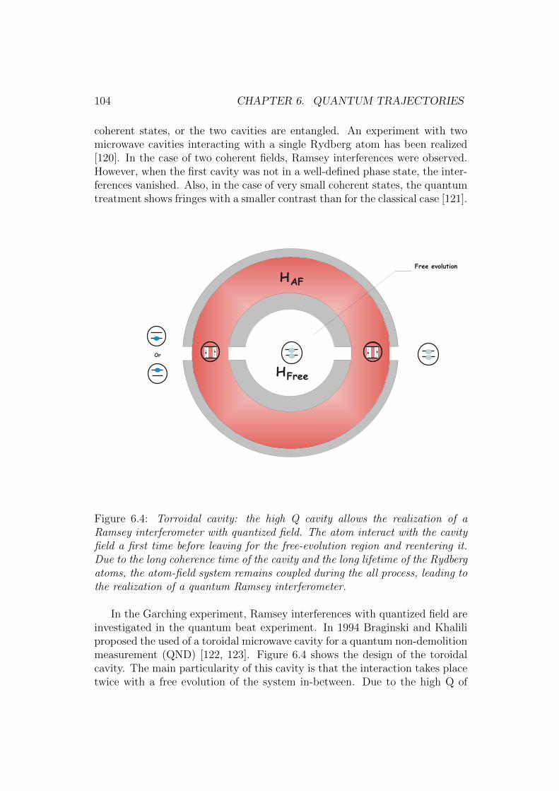
104 CHAPTER 6. QUANTUM TRAJECTORIES
coherent states, or the two cavities are entangled. An experiment with twomicrowave cavities interacting with a single Rydberg atom has been realized[120]. In the case of two coherent fields, Ramsey interferences were observed.However, when the first cavity was not in a well-defined phase state, the inter-ferences vanished. Also, in the case of very small coherent states, the quantumtreatment shows fringes with a smaller contrast than for the classical case [121].
Or
Free evolution
HAF
HFree
Figure 6.4: Torroidal cavity: the high Q cavity allows the realization of aRamsey interferometer with quantized field. The atom interact with the cavityfield a first time before leaving for the free-evolution region and reentering it.Due to the long coherence time of the cavity and the long lifetime of the Rydbergatoms, the atom-field system remains coupled during the all process, leading tothe realization of a quantum Ramsey interferometer.
In the Garching experiment, Ramsey interferences with quantized field areinvestigated in the quantum beat experiment. In 1994 Braginski and Khaliliproposed the used of a toroidal microwave cavity for a quantum non-demolitionmeasurement (QND) [122, 123]. Figure 6.4 shows the design of the toroidalcavity. The main particularity of this cavity is that the interaction takes placetwice with a free evolution of the system in-between. Due to the high Q of
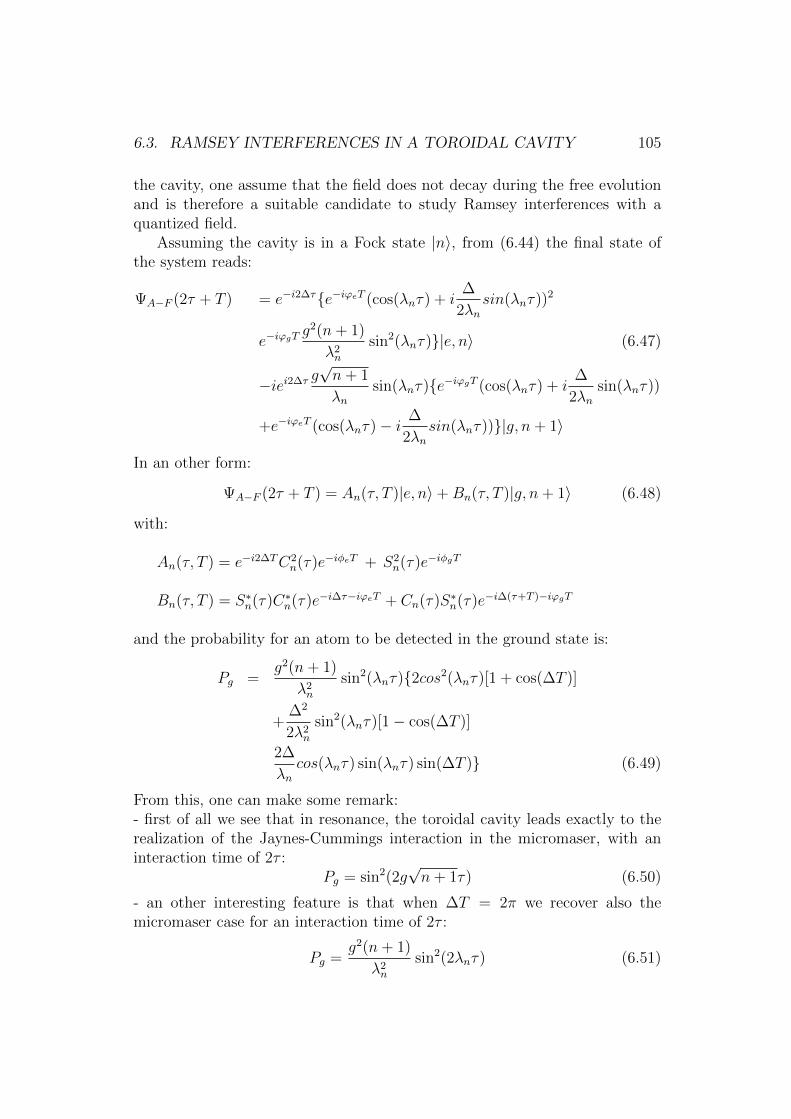
6.3. RAMSEY INTERFERENCES IN A TOROIDAL CAVITY 105
the cavity, one assume that the field does not decay during the free evolutionand is therefore a suitable candidate to study Ramsey interferences with aquantized field.
Assuming the cavity is in a Fock state |n〉, from (6.44) the final state ofthe system reads:
ΨA−F (2τ + T ) = e−i2∆τe−iϕeT (cos(λnτ) + i∆
2λnsin(λnτ))2
e−iϕgTg2(n+ 1)
λ2n
sin2(λnτ)|e, n〉 (6.47)
−iei2∆τ g√n+ 1
λnsin(λnτ)e−iϕgT (cos(λnτ) + i
∆
2λnsin(λnτ))
+e−iϕeT (cos(λnτ)− i ∆
2λnsin(λnτ))|g, n+ 1〉
In an other form:
ΨA−F (2τ + T ) = An(τ, T )|e, n〉+Bn(τ, T )|g, n+ 1〉 (6.48)
with:
An(τ, T ) = e−i2∆TC2n(τ)e−iφeT + S2
n(τ)e−iφgT
Bn(τ, T ) = S∗n(τ)C∗n(τ)e−i∆τ−iϕeT + Cn(τ)S∗n(τ)e−i∆(τ+T )−iϕgT
and the probability for an atom to be detected in the ground state is:
Pg =g2(n+ 1)
λ2n
sin2(λnτ)2cos2(λnτ)[1 + cos(∆T )]
+∆2
2λ2n
sin2(λnτ)[1− cos(∆T )]
2∆
λncos(λnτ) sin(λnτ) sin(∆T ) (6.49)
From this, one can make some remark:- first of all we see that in resonance, the toroidal cavity leads exactly to therealization of the Jaynes-Cummings interaction in the micromaser, with aninteraction time of 2τ :
Pg = sin2(2g√n+ 1τ) (6.50)
- an other interesting feature is that when ∆T = 2π we recover also themicromaser case for an interaction time of 2τ :
Pg =g2(n+ 1)
λ2n
sin2(2λnτ) (6.51)
106 CHAPTER 6. QUANTUM TRAJECTORIES
This feature is also in accord with the Ramsey interference with classical field.The implementation of the QTM for the torroidal cavity is then straight
forward. From equation (6.48), the two jumps operator C1 and C0 can berewritten as:
C1 =
√Ra†√
a†a+ 1Bn(τ, T ) (6.52)
andC0 =
√RAn(τ, T ) (6.53)
The numerical simulation is then realized as outlined in the section 6.1.Figure 6.5 shows the simulation for an initial thermal state with < nth >= 1.5,R = 100, and τ = T/2 = 66 µs.
0 50 100 150 200 250 300 350 40020
40
60
80
100
120
140
160
180
0 50 100 150 200 250 300 350 4000
10
20
30
40
50
60
70
Frequency Detuning (MHz)
Detected Ground State Atom
Detected Excited State Atom
Figure 6.5: Quantum Ramsey Interferences in a torroidal cavity
Outlook
In this thesis, the experimental results, where the ground state of a two-levelatomic system interacts with a single mode of a high Q cavity, are presented.A new laser system to promote 85Rb atoms into the Rydberg maser groundstate 61D5/2 is developed and major improvements on the cryogenic systemare achieved.
With a better control of the still temperature in the dilution cryostat andthe addition of extra heat shielding around the experimental environment,the end-temperature is improved by a factor of two at ∼ 150 mK. Moreover, acontinuous working temperature from 150 mK to 1.3 K is possible, opening thepath for the observation of quantum stochastic resonances in the micromaser.
The development of a new laser setup using a two-step diode laser systemopened the possibility of exciting maser ground states that have never be donein this setup until now. We have also shown that purely optical spectroscopy ofRb Rydberg states is possible in a room-temperature gas cell in three differentexcitation schemes using the quantum amplification of the electron shelving.The excitation of Rydberg states is monitored by observing the absorption ofthe laser driving the strongest transition. The spectroscopy method developedin this thesis can be used to detect Rydberg states with high frequency reso-lution and can be therefore the basis for convenient stabilization setups for awide range of experiments. Especially, ultracold Rydberg gases are a promis-ing candidate for realizing controlled quantum gates in atomic ensembles. Im-provements in excitation and detection techniques and especially methods tostabilize laser to specific Rydberg transitions are therefore important in manyexperiments. Finally, the Rydberg transitions in a gas cell are highly immuneto a linear and quadratic DC Stark shift. If magnetic fields are shielded bya µ-metal cover, the Rydberg lines in a cell are as stable as low-lying Rb lev-els. The closely spaced Rydberg levels therefore form a dense comb of atomiclines which offers interesting possibilities for frequency metrology and coherentcontrol applications.
Finally, experiments with ground states atoms have been performed forthe first time in the one-atom-maser. Measurements of the magnetic fieldcompensation have achieved a higher contrast and Stark effect experiments
107
108 CHAPTER 6. QUANTUM TRAJECTORIES
with high lying D state have been performed. The frequency shift of the61D5/2 level in presence of small DC electrical field has been measured witha time of flight experiment leading to an evaluation of the fourth-order Starkeffect for the 61D state in 85Rb.
The interaction between the maser ground state and the cavity field hasbeen investigated for both a low atomic injection rate and a high atomic pump-ing leading to the measurement of the first maserlines in this configuration.The first observation of Rabi oscillations, with a high contrast, where groundstate atoms interact with the quantized thermal field of the cavity, gives im-portant informations about the actual field temperature.
Sending either excited state atoms or ground state atoms inside the cavityopens the possibility for a wide range of new experiments. Among them, thegeneration of more robust trapping states is possible by mixing excited andground states atoms in the atomic injection. Also pump-probe experimentscould be realized. Sending a sequence of excited atoms prepares the cavity ina well defined quantum state. The generated field state can then be probedwith ground state atoms. At low injection rate with less than one groundstate atom per cavity decay time, the realization of Rabi oscillations with highnumber Fock-state is possible. At higher injection rate, the quantum fieldgenerated in the cavity can be used for atom-atom entanglement.
Bibliography
[1] A. Einstein, Phys. Zeitschr., 18, 121 (1917)
[2] V. Weisskopf and F. Wigner, Z. Phys., 63 54 (1930)
[3] W.E. Lamb Jr. and R.C. Retherford, Phys. Rev., 72, 241 (1947)
[4] H.A. Bethe, Phys. Rev., 72, 339 (1947)
[5] R. Pohl et al., The Muonic Hydrogen Lamb-Shift Experiment, Proceed-ings of the EXA05, eds. A. Hirtl, J. Marton, E. Widmann and J. Zmeskal,Austrian Academy of Sciences Press, Vienna, p. 285 (2005)
[6] E. T. Jaynes and F. W. Cummings, IEEE J. Quant: Elec 51 89 (1963)
[7] E.M Purcell, Phys. Rev., 69, 681 (1946)
[8] H.B.G Casimir and D. Polder, Phys. Rev., 73, 360 (1948)
[9] G. Rempe et al., Coherences and Quantum Optics VIII, Kluwer Academic/ Plenum Publishers, New York, p. 241(2003)
[10] J. Clarke and F.K. Wilhem, Nature, 453, 1031 (2008)
[11] G. Burkard et al., Phys. Rev. Lett., 83, 4204 (1999)
[12] J.A Gallas, G. Leuchs, H. Walther and H. Finger(1985), Advances inAtomic and Molecular Physics, Vol.20, Academic Press, New York, p.413
[13] S. Haroche and J.M Raymond, (1985), Advances in Atomic and MolecularPhysics, Vol.20, Academic Press, New York, p.350
[14] P. Filipowicz, J. Javanainen and P. Meystre, Phys. Rev. A, 34, 3077(1986)
[15] S.Brattke, B.T.H. Varcoe and H. Walther, Phys. Rev. Lett., 86, 3534(2001)
109
110 BIBLIOGRAPHY
[16] O.Benson, G. Raithel and H. Walther, Phys. Rev. Lett., 72, 3506 (1994)
[17] J. Ye, H.J. Kimble and H. Katori, Science, 320, 1734 (2008)
[18] R. Blatt and D. Wineland, Nature, 453, 1016 (2008)
[19] H. Dehmelt, IEEE Trans. Instrum. Meas., 31, 83 (1982)
[20] P. Thoumany, T.W. Hansch, G. Stania, L. Urbonas and Th. Becker, Opt.Lett., 34, 1621 (2009)
[21] P. Thoumany, T. Germann, T.W. Hansch, G. Stania, L. Urbonas and Th.Becker, J. of Mod. Opt., 56, 2055 (2009)
[22] G.Feher et al., Phys. Rev., 109, 221 (1958)
[23] K.H. Drexhage, H. Kuhn and F.D. Schafer, Ber. Bunsen Ges. Phys, 72,329(1968)
[24] D. Meschede, H. Walther and G. Muller, Phys. Rev. Lett., 54, 551 (1985)
[25] J.C. Slater, Microwave Electronics (Princeton, N.J.: Van Nostrand, 1950)
[26] B-G. Englert, Elements of Micromaser Physics, 1994
[27] F. Bloch and A. Siegert, Phys. Rev., 57, 522 (1940)
[28] G. Rempe , H. Walther and N. Klein, Phys. Rev. Lett., 58, 353 (1987)
[29] B.T.H Varcoe, S. Brattke, M. Weidinger, H. Walther, Nature, 403, 743(2000)
[30] L.Urbonas, Experiments with the One-Atom-Maser, Dissertation,Ludwig-Maximilians-Universitat, Munchen (2009)
[31] P. Lougovski et al., Phys. Rev. Lett., 78, 2547 (2003)
[32] D. Suter, The Physics of Laser-Atom Interactions, Cambrige UniversityPress, (1997)
[33] L.A. Luigiato, M.O. Scully and H. Walther, Phys. Rev. A, 36, 740 (1987)
[34] H.J Carmichael, Statistical Methods in Quantum Optics 1, Springer(1999)
[35] G. Rempe and H. Walther, Phys. Rev. A, 42, 1650 (1990)G.Rempe, F. Schmidt-Kaler and H. Walter, Phys. Rev. Lett., 64, 2783(1990)
BIBLIOGRAPHY 111
[36] J.P. Gordon, H.J. Zeiger and C.H. Townes, Phys. Rev., 95, 282 (1954)J.P. Gordon, H.J. Zeiger and C.H. Townes, Phys. Rev., 99, 1264 (1955)
[37] C. Kittel, Introduction to Solid State Physics, J. Wiley and Sons, NewYork, 7th Edition (1996)
[38] G. Babst, Aufbau und Test eines Mikromaser mit Supraleiten-den Resonator im Temperaturbereich von 0.5K, Dissertation,Ludwig-Maximilians-Universitat, Munchen (1989)
[39] T. Muller-Seidlitz, Untersuchungen am Ein-Atom-Maser, Dissertation,Ludwig-Maximilians-Universitat, Munchen (1992)
[40] C.T. Bodendorf et al., Phys. Rev. A, 57, 1371 (1998)M.S. Kim et al., Phys. Rev. A, 58, R65 (1998)
[41] N.F. Ramsey, Molecular Beams, Clarendon Oxford (1956)
[42] G. Marchi, Construction of an Apparatus for the Measurement of thePhase Diffusion in the Micromaser, Dissertation, Universita Degli Studidi Milano (2003)
[43] J. Rydberg, Phil. Mag. 5th series, 29, 331, (1890)
[44] A. Dalgarno, Rydberg Atoms in Astrophysics, in Rydberg States of Atomsand Molecules, edited by R.F. Stebbings and F.B. Dunning, CambridgeUniversity Press, (1983)
[45] P. Koch, Rydberg studies using fast beams, in Rydberg States of Atomsand Molecules, edited by R.F. Stebbings and F.B. Dunning, CambridgeUniversity Press, (1983)
[46] T. Cubel, et al., Phys. Rev. A, 72, 023405 (2005)
[47] M. Seaton, Quantum defect theory, Rep. Prog. Phys., 46, 167, (1983)
[48] B. Sanguinetti et al. , J. Phys. B, 42, 165004 (2009)
[49] T.F. Gallagher, Rydberg Atoms, Cambridge University Press, (1994)
[50] L.G. D’yachkov and P.M. Pankratov, J. Phys. B, 24, 2267 (1991)
[51] B. Oumarou, et al., Phys. Rev. A, 37, 1885 (1988)
[52] A.R. Edmonds, et al., J. Phys. B, 12, 2781 (1979)
112 BIBLIOGRAPHY
[53] W. Lange, Koharent angeregte Rydberg-Atome in einem resonator-modifizierten Vacuumfeld, Dissertation, Ludwig-Maximilians-Universitat,Munchen (1994)
[54] I.I. Beterov et al., Phys. Rev. A, 79, 052504 (2009)
[55] A.L. de Oliveira et al., Phys. Rev. A, 65, 031401(R) (2002)
[56] F. Gounand, J. Phys. (Paris), 40, 457 (1979)
[57] C.E. Theodosiou, Phys. Rev. A, 30, 2881 (1984)
[58] M.L. Zimmerman, Phys. Rev. A, 20, 2251 (1979)
[59] D.H. Tuan, S. Liberman and J. Pinard, Opt. Com., 18, 533 (1976)
[60] D. Meschede, Strahlungwechselwirkung von Rydbergatomen Realisierungeines Ein-Atom-Maser, Dissertation, Ludwig-Maximilians-Universitat,Munchen (1984)
[61] J.D. Jackson, Classical Electrodynamics, J. Wiley Verlag, third editioncollection (1999)
[62] W. Buckel, Superconductivity - Fundamentals and Applications, J. WileyVerlag, second edition (2007)
[63] A.N. Luiten (editor), Frequency Measurement and Control, vol. 79 ofTopics in Applied Physics, Springer (2001)
[64] G. Muller, Supraleitende Niobresonatoren im Millimeterwellenbereich,Dissertation, Bergishe Universitat - Gesamthochschule Wuppertal (1983)
[65] M.A. Allen, et al. , Superconducting Niobium Cavity Measurements atSLAC, IEEE Transactions on Nuclear Science, 18 (3), 168 (1971)
[66] N. Klein, Supraleitende Mikrowellenresonatoren fur Anwendungen inphysikalischen Grundlagenexperimenten, Externer Bericht, WUB-DIS 89-3, Bergishe Universitat - Gesamthochschule Wuppertal (1989)
[67] R.P. Heerlein, Entwicklung von neuartigen Mikrowellenresonatoren furden Ein-Atom-Maser, Diplomarbeit, Ludwig-Maximilians-Universitat,Munchen (1998)
[68] T.R. Roberts and S.G. Sydoriak, Phys. Rev., 98, 1672 (1955)
[69] G. Batey, V. Mikheev, J. Low Temp. Phys., 113, 933 (1998)
BIBLIOGRAPHY 113
[70] H. London, Proc. 2nd Int.Conf. on Low Temp. Phys. (Oxford Univ. Press,London 1951), 157
[71] D.J. Cousins et al. , J. Low Temp. Phys., 114, 547 (1999)
[72] A. Buchleitner and R. Mantega, Phys. Rev. Lett., 80, 3932 (1998)
[73] J. Bernu et al. , Phys. Rev. Lett., 101, 180402 (2008)
[74] G. Raithel, Habilitation, Ludwig-Maximilians-Universitat, Munchen ,(1995)
[75] J.M. Pierce, Methods of Experimental Physics, vol. 11, Academic Press,New York, p. 541 (1973)
[76] H. Padamsee, K. Shepard and R. Sundelin, Physics and Accelerator Ap-plications of RF Superconductivity, Annu. Rev. Nucl. Part. Sci., 43, 635(1993)
[77] W. Hanle, Uber magnetische Beeinflussung der Polarisation der Reso-nanzfluoreszenz, Zeitschrift fur Physik, 30, 93 (1924)
[78] C.T. Bodendorf, Untersuchungen am Ein-Atom-Maser mit externerEinkopplung, Dissertation, Ludwig-Maximilians-Universitat, Munchen(2000)
[79] S.Brattke, Untersuchung von Photonenzahlzustanden mit dem Ein-Atom-Maser, Dissertation, Ludwig-Maximilians-Universitat, Munchen (2001)
[80] T. Germann, Experimente fur den Ein-Atom-Maser mit Hilfe eines3-stufigen Diodenlaser-Systems, Diplomarbeit, Ludwig-Maximilians-Universitat, Munchen (2008)
[81] R.T. Hawkins et al., Phys. Rev. A, 15, 967 (1977)
[82] T.F. Gallagher et al., Phys. Rev. A, 15, 1937 (1977)
[83] T.F Gallagher and W.E. Cooke, Phys. Rev. A, 18, 2510 (1978)
[84] P. Kulina and R-H Rinkleff, J. Phys. B: At. Mol. Phys., 18, 245 (1984)
[85] U. Fano and J.W. Cooper, Rev. Mod. Phys, 40, 441 (1965)
[86] G. Marchi, Construction of an Experimental Apparatus for the Measure-ment of the Phase Diffusion in the Micromaser, Tesi di Dottorato, Uni-versita degli Studi di Milano
114 BIBLIOGRAPHY
[87] T. Meunier et al., Phys. Rev. Lett., 94, 010401 (2005)M. Brune et al., Phys. Rev. Lett., 76, 1800 (1996)
[88] M. Saffman, T.G. Walker and K. Mølmer, Reviews of Modern Physics,82, 2313 (2010)
[89] D. Jaschke et al., Phys. Rev. Lett., 85, 2208 (2000)
[90] G. M. Lankhuijzen and L. D. Noordam, Adv. At., Mol., Opt. Phys., 38,121 (1998)
[91] D.J. Bradley et al., J. Phys. B, 6, 1594 (1973)
[92] J.R. Rubbmark et al., J. Phys. B, 10, 421 (1977)
[93] M. Auzinsh et al., Opt. Commun., 264, 333 (2006)
[94] L. Lorini et al., ”Recent Atomic Clock Comparisons at NIST”, EUr. Phys.J. Special Topics, 163, 19 (2008)
[95] A.K. Mohapatra, T.R. Jackson and C.S. Adams, Phys. Rev. Lett., 98,113003 (2007)
[96] S. Mauger, J. Millen and M. P. A. Jones, J. Phys. B, 40, F319 (2007)
[97] B.P. Stoicheff and E. Weinberger, Phys. Rev. Lett., 44, 733 (1980)
[98] F. Nez et al., Opt. Commun., 102, 432 (1993)
[99] H.J. Metcalf and P. van der Straten, Laser Cooling, Springer New York(1999)
[100] M. Rotenberg et al., the 3-j and 6-j Symbols, Technology Press, Mas-sachusetts Institute of Technology Cambridge MA, (1959)
[101] A.K. Mohapatra et al., Nature Physics, 4, 890 (2008)
[102] P. Meystre and E.M. Wright, Phys. Rev. A, 37, 2524 (1988)
[103] C. Wagner, R.J. Brecha, A. Schenzle and H. Walther, Phys.Rev. A, 47,5068 (1993)
[104] J. Dalibard, Y. Castin and K. Molmer, Phys. Rev. Lett., 68, 580 (1992)
[105] C.W. Gardinger, A.S . Perkins and P. Zoller, Phys. Rev. A, 46, 4382(1992)
BIBLIOGRAPHY 115
[106] H.J Carmichael, An Open System Approach to Quantum Optics,Springer (1993)
[107] J.D. Cresser and S.M Pickles, Quantum Semiclass. Opt., 8, 73-104 (1996)
[108] H.M Wiesman, Phys. Rev. A, 49, 2133 (1994)
[109] A. Liebman and G. J. Milburn, Phys.Rev. A, 51, 736 (1995)
[110] F. Casagrande, A. Lulli and S. Ulzega, Phys .Rev. A, 60, 1582 (1999)
[111] M.O. Scully and al., Phys. Rev. A, 44, 5992 (1991)
[112] T. Quang et al., Phys. Rev. A, 48, 803 (1993)
[113] J.D. Cresser, Phys.Rep., 94, 47 (1983)
[114] M.O. Scully and W.E. Lamb, Phys. Rev., 159, 208 (1967)
[115] F. Casagrande et al., Phys. Rev. Lett., 90, 183601 (2003)
[116] S. Deleglise et al., Nature, 455, 510 (2008)
[117] N.F. Ramsey, Phys. Rev., 78, 695 (1950)
[118] L. Essen and J.V.L. Parry, Nature, 176, 280 (1955)
[119] M.M. Salour and C. Cohen-Tannoudji, Phys. Rev. Lett., 38, 757 (1977)J.C. Bergquist, S.A. Lee and J.L. Hall, Phys. Rev. Lett., 38, 159 (1977)
[120] P. Bertet et al., Nature, 411, 166 (2001)
[121] G.S. Agarwal, P.K. Pathak and M.O. Scully, Phys. Rev. A, 67, 043807(2003)
[122] V.B. Braginsky, F.Ya. Khalili, Phys. Lett. A, 186, 15 (1994)
[123] M.P. Klembovsky, M.L. Gorodetsky and T. Becker, JETP Lett., 79, 550(2004)

116 BIBLIOGRAPHY
Acknowledgment
This work has been possible through the contributions of many people both atthe scientific and at a more personal level. Therefore, I would like to thanksthem for all their supports during my researchs.
I deeply thank Prof. Herbert Walther, for the opportunity to work on thisbeautiful Micromaser experiment.
I am very thankful to Prof. Theodor W. Hansch, who agreed to continuemy supervision after the death of Prof. Walther, providing a very motivatingenvironment with new perspectives to continue my PhD.
A special thanks to Dr. Thomas Becker. For his support from the firstday, as I started as an internship student till the end of this manuscript, forall the advices, discussions, constructive comments, new ideas and the finalcorrection of this work.
A particular thanks goes to Prof. Pavel Lougovski, for the great friendshipstarted in an office at MPQ, the collaborations and discussions over the yearsand for valuable comments on earlier versions of this thesis.
I am also very thankful to Dr. Linas Urbonas, Dr. Gabriele Marchi, Dr.Gernot Stania, Mikhael Klembowsky and Dr. Bruno Sanguinetti, who workedwith me over the last years, for their positive input and valuable advices.
I also thank all my colleagues at MPQ for the wonderful working atmo-sphere here, the funny coffee break and in particular Dr. Maria Eckholt, itwas very interesting and funny to organize conferences with you.
I also want to thank Mrs. Hermann and all the administrative staff of MPQwho make any bureaucratic work much easier for me. Also a special thanks toMrs. Faß from the LMU for the help in the management of my Marie CurieFellowship.
I am thankful to Mr. Thomas Strobl and the MPQ workshop who alwaysmanaged to realize high precise work from my not so accurate drawings.
On a more personal level, I would to thank my parents and my brotherwho always supported me during all these years abroad.
Finally, I would like to thanks all my friends for their support during allthese years and especially Giovanna for her presence and patience. Withoutyou, would have been everything more complicated.
117


![ISSN 0280-316X10520/...cavity quantum electrodynamics, or shortly cavity QED [2]. As with any physical As with any physical model, the degrees of freedom that are not important for](https://static.fdocuments.net/doc/165x107/5f76355d4bc22f497a18e973/issn-0280-316x-10520-cavity-quantum-electrodynamics-or-shortly-cavity-qed-2.jpg)


![Free Space QED with a Single Rydberg Superatom [1]...Free Space QED and Emergent Universal Dynamics with a Single Rydberg Superatom Jan Kumlin1, Sebastian Ho˜erberth2, and Hans Peter](https://static.fdocuments.net/doc/165x107/609276a4cc59352aa21a55be/free-space-qed-with-a-single-rydberg-superatom-1-free-space-qed-and-emergent.jpg)