Optical Remote Sensing for Emission Characterization from Non … · 2015-08-28 · Optical Remote...
44
FINAL ORS Protocol June 14, 2006 1 Optical Remote Sensing for Emission Characterization from Non-point Sources 1.0 Scope and Application 1.1 Introduction. This protocol provides the user with methodologies for characterizing gaseous emissions from non-point pollutant sources. These methodologies use an open-path, Path-Integrated Optical Remote Sensing (PI-ORS) system in multiple beam configurations to directly identify “hot spots” and measure emission fluxes. Basic knowledge of a PI-ORS system and the ability to obtain quality path-integrated concentration (PIC) data is assumed. The user must be capable of using commercial software to utilize the procedures and algorithms explained in this protocol. The methodologies in this protocol have been well developed, evaluated, demonstrated, validated, and peer-reviewed. 1-12 NOTE 1 — Any mention of a “PI-ORS system” in this protocol refers to the open-path PI-ORS instrument itself, as well as any associated components used, such as mirrors, scanners, and software. This protocol does not discuss specific applications (e.g., hog farms, landfills), but provides general guidelines or procedures that can be applied. Detailed protocols for specific applications may be added at a future date. 1.1.1 Scope. This protocol currently describes three methodologies, each for a specific use. The Horizontal Radial Plume Mapping (HRPM) methodology was designed to map pollutant concentrations in a horizontal plane. The Vertical Radial Plume Mapping (VRPM) methodology was designed to measure mass flux of pollutants through a vertical plane, downwind from an emission source. The one-dimensional Radial Plume Mapping methodology (1D-RPM) was designed to profile pollutant concentrations along a line-of- sight (e.g., along an industrial site fenceline). In future revisions to this protocol, additional PI-ORS emission monitoring methodologies (other than the methodologies described in this protocol) that address non-point sources can be added as validation data are generated. 1.1.2 Choice of Instrumentation. The choice of PI-ORS system to be used for the collection of measurement data (and subsequent calculation of PIC) is left to the discretion of the user, and should be dependent on the compounds of interest and the purpose of the study. The methodologies are independent of the particular PI-ORS system used to generate the PIC data. It is recommended for the HRPM, VRPM, and 1D-RPM methodologies that the typical expected concentration over the longer beams should be about 10 times the minimum detection limit of the instrument. When this is not the case, the user should replace nondetects with values of half the minimum detection limit (see Table A.3 in the Appendix A).
Transcript of Optical Remote Sensing for Emission Characterization from Non … · 2015-08-28 · Optical Remote...
FINAL ORS ProtocolJune 14, 2006
1
Optical Remote Sensing for Emission Characterization from Non-point Sources
1.0 Scope and Application
1.1 Introduction. This protocol provides the user with methodologies for characterizing gaseous emissions from non-point pollutant sources. These methodologiesuse an open-path, Path-Integrated Optical Remote Sensing (PI-ORS) system in multiple beam configurations to directly identify “hot spots” and measure emission fluxes. Basic knowledge of a PI-ORS system and the ability to obtain quality path-integrated concentration (PIC) data is assumed. The user must be capable of using commercial software to utilize the procedures and algorithms explained in this protocol. Themethodologies in this protocol have been well developed, evaluated, demonstrated,validated, and peer-reviewed.1-12
NOTE 1 — Any mention of a “PI-ORS system” in this protocol refers to the open-path PI-ORS instrument itself, as well as any associated components used, such as mirrors, scanners, and software.
This protocol does not discuss specific applications (e.g., hog farms, landfills), but provides general guidelines or procedures that can be applied. Detailed protocols for specific applications may be added at a future date.
1.1.1 Scope. This protocol currently describes three methodologies, each for a specific use. The Horizontal Radial Plume Mapping (HRPM) methodology was designed to map pollutant concentrations in a horizontal plane. The Vertical Radial Plume Mapping (VRPM) methodology was designed to measure mass flux of pollutants through a vertical plane, downwind from an emission source. The one-dimensional Radial Plume Mappingmethodology (1D-RPM) was designed to profile pollutant concentrations along a line-of-sight (e.g., along an industrial site fenceline). In future revisions to this protocol, additional PI-ORS emission monitoring methodologies (other than the methodologies described in this protocol) that address non-point sources can be added as validation data are generated.
1.1.2 Choice of Instrumentation. The choice of PI-ORS system to be used for the collection of measurement data (and subsequent calculation of PIC) is left to the discretion of the user, and should be dependent on the compounds of interest and the purpose of the study. The methodologies are independent of the particular PI-ORS system used to generate the PIC data. It is recommended for the HRPM, VRPM, and 1D-RPMmethodologies that the typical expected concentration over the longer beams should be about 10 times the minimum detection limit of the instrument. When this is not the case, the user should replace nondetects with values of half the minimum detection limit (see Table A.3 in the Appendix A).
FINAL ORS ProtocolJune 14, 2006
2
1.1.3 Developmental Basis. Several methodologies have been developed and applied to estimate emission rates from non-point fugitive sources — such as landfills, coal mines, and wastewater treatment plants — using PI-ORS technologies.3, 13-18 The methodologies explained in this protocol were developed from studies that concentrated on developing, evaluating, and demonstrating the various configurations of the radial plume mapping (RPM) basedmethodologies.1,2,4-7,9-11 The RPM-based methodologies (configurations, procedures, and algorithms) were patented as a technology for mapping air contaminants using a PI-ORS system with a non-overlapping, variable pathlength, radial beam geometry.8 The RPM methodologies are the intellectual property of the University of Washington; if you plan to employ the RPM-based methodologies, please contact the Office of Intellectual Property and Technology Transfer at The University of Washington (UW TechTransfer; [email protected]) for potential licensing.
1.1.4 Applicability. The methodologies described in this protocol are appropriate for characterizing ground level area sources and non-point fugitive emission sources such as landfills, lagoons, and industrial complexes. The limitations of these methodologies can be based on the instrument or beam geometry.
1.1.4.1 Instrument-Specific Limitations. The PI-ORS system chosen will determine the maximum pathlength, the compounds that can be detected, and the detection limits of these compounds and can influence accuracy and precision as well.
1.1.4.2 Beam Geometry Limitations. Plume emissions are assumed to originate near ground level (within three meters from the ground). If some or all of the emissions are above the three-meter criteria, then the beam geometries explained in this protocol may need to be modified. Complex topography and obstructions may require some variations from the standard configurations described in this protocol.
1.2 Compound List. Any fugitive gaseous compound is a potential candidate for application of these methodologies. These methodologies are restricted only by the limitations of the PI-ORS system chosen.
1.2.1 Sensitivity. Table 1 shows some typical sensitivity ranges for several PI-ORS systems. Prior to field deployment, the expected sensitivity of the PI-ORS system should be evaluated against project goals.
1.2.2 Data Quality. The level of acceptable uncertainty is dependent on the application of the reported data – whether for hot spot determination (HRPM), measurement of emissions flux (VRPM), or line-of-sight profile concentrations (1D-RPM). The user must tailor their choice of PI-ORS system, configuration, and tolerance parameters to meet their end needs.

FINAL ORS ProtocolJune 14, 2006
3
Table 1. Typical Sensitivity Ranges for Several PI-ORS Systems
PI-ORS System*
Formal-dehyde
1,3-Butadiene
Acrolein Benzene Ammonia Total VOC
Scanning OP-FTIR (for > 100 m pathlength)
2 – 10 ppb
2 – 10 ppb 8 – 30 ppb
15 – 50 ppb
0.5 – 4 ppb 1 – 5 ppb
UV-DOAS(for > 250 m pathlength)
0.5 ppb NA NA 0.1 ppb 1 ppb NA
TDLAS (for > 250 m pathlength)
NA NA NA NA 20 – 50 ppb
NA
PI-DIAL(1000 m pathlength)
** ** ** 10µg/m3
** **
* See Section 6 for full instrument names.NA This compound cannot currently be measured with this instrument.** Typically a custom-built instrument. Sensitivity ranges are instrument-specific.
2.0 Summary of Methodologies
2.1 Principle. This protocol describes the application of the HRPM, VRPM, and 1D-RPM methodologies designed specifically for the use of PI-ORS systems. The HRPM methodology utilizes multiple non-intersecting beam paths in a horizontal plane and optimizing algorithms to give a time-averaged surface concentration field across plumes of contaminants. This methodology is used to locate hot spots close to the ground. The VRPMmethodology utilizes multiple non-intersecting beam paths in a vertical plane downwind from the emission source to obtain a mass-equivalent plume map. This map, in conjunction with wind speed and direction, is used to obtain the flux of pollutants through the vertical plane. The measured flux is then used to estimate the emission rate of the upwind sourcebeing characterized. The 1D-RPM methodology utilizes multiple beam paths along a line-of-sight to obtain concentration profiles downwind of a source (e.g., along an industrial site fenceline). The peak concentration position along the line-of-sight can be incorporated with wind direction to estimate the location of an upwind fugitive emission source.
2.1.1 The user-selected PI-ORS system collects spectral data; there are no true “samples” that require preservation, storage, transport, extraction, digestion, or concentration. The chemical concentration of each gas species of interest along each beam path is obtained following the measurement and analysis procedures for the instruments being used.
2.1.2 The physical range and sensitivity of the methodologies are determined by the limitations of the PI-ORS system selected to acquire the PIC data. The accuracy of theresults from the methodologies depends on the instrument accuracy as well as: 1) the quality control (QC) criteria defined for the methodology-specific algorithms, and 2) the accuracy and representativeness of the wind data (for VRPM and 1D-RPM methodologies).

FINAL ORS ProtocolJune 14, 2006
4
2.2 HRPM Methodology – Hot Spot Source Location. The HRPM methodology is used to locate the source of fugitive emissions or hot spots. A rectangular area (which may be a square) is defined around the ground location where the suspected gaseous emissionsare originating. Ideally, the HRPM configuration will cover the entire suspected source area; however, this may be prevented by equipment limitations or site conditions. Larger areas may need to be divided into smaller sections and studied separately.
2.2.1 Once the HRPM configuration area has been defined, it is divided into smaller rectangular areas called pixels. The total number of pixels required is less than or equal to the total number of beam paths. Each pixel will have at least one optical beam path that terminates within its boundaries by a pathlength-defining component (PDC).
NOTE 2 — The methodologies here are not instrument specific. For ease of presentation, pathlength-defining component (PDC) is used to denote the component on the other end of the optical path from the PI-ORS instrument. Depending on the instrument selected, this could be a source, detector, mirror, or other reflecting object.
2.2.2 The scanning PI-ORS instrument is typically placed on a corner of the rectangular sampling area. The reconstruction algorithm for obtaining concentration contour maps consists of two stages (detailed in Section 12.2).
NOTE 3 — Although the PI-ORS instrument is typically placed on a corner of the rectangular sampling area, in some cases it may be necessary to place the PI-ORS instrument along a boundary of the survey area. This protocol does not address alternate placement of the PI-ORS instrument.
2.2.2.1 An iterative inversion algorithm is used to determine average concentrations in each pixel.
2.2.2.2 An interpolation procedure is then applied to these concentration values to calculate concentrations in higher spatial resolution.
2.2.3 HRPM calculations are performed and the locations of concentration maxima qualitatively indicate the locations of gaseous emission hot spots. Wind speed and direction measurements may be recorded while collecting HRPM methodology data to aid in interpreting the concentration contour maps produced.
2.3 VRPM Methodology - Estimation of Emission Rate. The VRPM methodology is used to estimate the rate of gaseous emissions from an area fugitive source. A vertical scanning plane, downwind of the source, is used to directly measure the gaseous flux (detailed in Section 12.3).
2.3.1 The total length of the measurement area required depends on the size of the emission source, as well as the limitations of the selected PI-ORS system.
2.3.2 The height of the scanning area is dependent on the PI-ORS system limitations, the distance to the upwind boundary of the source, and the limitations of the infrastructure

FINAL ORS ProtocolJune 14, 2006
5
used for mounting the PI-ORS system components (e.g., mirrors and/or meteorological station).
2.3.3 Wind speed and direction measurements must be recorded for flux calculations and preferably should be monitored in at least two heights (usually at 2 and 10 meters) for a more accurate interpolation and extrapolation through the height of the vertical plane. Inspecial cases when two wind monitors are not available, one wind monitor can be used at mid-height (3-5 m) to represent the average wind of the entire vertical plane. The VRPM method was validated with two wind monitors11; however, because a linear interpolation is applied between the two wind monitor heights, one wind monitor at mid-height should provide similar results.
2.3.4 The PIC measurements along the elevated beam paths (achieved by elevated PDC) provide vertical concentration gradient information of the emitted plume. The beam paths on the ground (ground level PDC) indicate the approximate ground levelconcentration profile along the length of the VRPM setup. Ground-level refers to the areaas close to horizontal as possible, relative to the surface of the measurement area.
2.3.5 A bivariate Gaussian function (or superposition of two) is assumed for the plume mass across the VRPM plane, and the parameters of the mass-equivalent bivariate Gaussian function(s) are reconstructed from the measured PIC. These reconstructed parameters are then used to calculate the concentration values across the VRPM plane at high resolution.
2.3.6 The concentration values (in ppm) are converted to mass concentrations usingthe molecular weight of the monitored gas species. The products of the mass concentration and the wind speed normal to the measurement plane are integrated across the plane to calculate the mass flux through the plane. Because the estimation of the emission rate is dependent on the wind data, stable and measurable wind conditions are desired so that the source remains upwind of the VRPM plane.
2.4 1D-RPM Methodology – Line-of-Sight Profile Concentrations and Upwind Source Location Estimation. The 1D-RPM methodology is used to profile pollutant concentrations along a line-of-sight downwind of a fugitive emission source. This pollutant concentration profile can be combined with wind data to estimate the location of an upwind source, when applicable. The scanning PI-ORS instrument and three or more PDC are placed in a crosswind direction along a line, such as an industrial site fenceline.
2.4.1 A Gaussian function (or superposition of two) is assumed for the plume concentration profile along the line-of-sight of the instrument and the parameters of the Gaussian function(s) are reconstructed from the measured PIC.
2.4.2 Multiple peak locations are reconstructed over time along the 1D-RPM line-of-sight. These peak positions are incorporated with corresponding wind directions to

FINAL ORS ProtocolJune 14, 2006
6
create back-projected vectors for each measurement period. When the back-projected vectors converge in an area, this indicates the probable location of an upwind hot spot.
3.0 Definitions
1D-RPM: One-dimensional Radial Plume Mapping. The 1D-RPM methodology is one of the three methodologies described in this protocol, and is used for reconstructing line-of-sight profile concentrations.
CCF: Concordance Correlation Factor. CCF is used to represent the quality of fit for the reconstruction in the path-integrated domain. CCF is similar to the Pearson correlation coefficient, but is adjusted to account for shifts in location and scale.
Cycle: Cycle is defined as one complete sequential data collection through all PDCs in the setup.
Gaussian function: A normal distribution curve with a specified mean and standard deviation.
HRPM: Horizontal Radial Plume Mapping. The HRPM methodology is one of the three methodologies described in this protocol, and is used for locating “hot spot” sources.
Kernel matrix: A matrix detailing the length of each beam path in each pixel of the HRPM plane.
NNLS: Non-negative least squares. NNLS is similar to a classical least square optimization algorithm, but is constrained to provide the best fit of non-negative concentration values used in the HRPM methodology.
PDC: Pathlength-defining components. PDC is used to denote the component on the other end of the optical path from the PI-ORS instrument. Depending on the instrument selected, this could be a source, detector, mirror, or other reflecting object.
PIC: Path Integrated Concentration. Given in the units of parts per million-meter (ppm-m), PIC is the integrated concentration of a gaseous pollutant measured along the beam pathlength.
PI-ORS: Path-Integrated Optical Remote Sensing. An instrument system used to acquire gaseous PIC data along an open optical beam path.
ppm: Parts per million. Typical units of gas concentration for PI-ORS instruments, ratioed by volume.
SBFM: Smooth Basis Functions Minimization. An algorithm used in the VRPM and1D-RPM methodologies to fit the parameters of the Gaussian basis function(s) to the measured PIC data.

FINAL ORS ProtocolJune 14, 2006
7
SSE: Sum of Squared Errors. The SSE is the sum of the squared differences between the measured and predicted PIC at each step of the iterative algorithm used in the VRPM and1D-RPM methodologies.
Tolerance parameter: A threshold value used to terminate iterative search algorithms of the methodologies described in this protocol.
VRPM: Vertical Radial Plume Mapping. The VRPM methodology is one of the three methodologies described in this protocol, and is used for estimation of the emission ratefrom an area source.
4.0 Interferences
4.1 General Interferences
4.1.1 Field-based interferences may result in the need to deviate from the setups specified for the PI-ORS system (see Section 11). Some examples of potential field-based interferences are vehicular or pedestrian traffic through the beam path and physical site obstructions (e.g., buildings, trees, and complex topography).
4.1.2 The methodologies described in this protocol are based on concentration analysis of the chosen PI-ORS system, and different instruments may have uniqueinterferences. For example, concentration determination may be affected by the presence of water vapor and carbon dioxide in the infrared, or oxygen and ozone in the UV. Detection levels for several compounds may increase with the presence of the interfering species.
4.2 Weather Interferences
4.2.1 General. Certain weather conditions such as rain, fog, or snow can obscure the light beam and affect the ability of the PI-ORS instrument to continuously measure gaseous concentrations. Transient, but significant, obscuration can occur during heavy precipitation events, particularly with longer path measurements. This could limit the sensitivity of the PIC measurements or the ability to collect data. All meteorological conditions are recordedin the field log so that the data collected during adverse conditions can be reviewed. The data collected during these events may be filtered out before inclusion in the methodologies calculations.
4.2.2 Winds. Wind conditions can greatly affect the results of field measurements and should be taken into account when interpreting data collected using the methodologies described in this protocol.
4.2.2.1 Calm wind conditions do not affect the HRPM methodology algorithm for hot spot source location. However, very low wind speeds are not ideal for the VRPM methodology for emission rate estimation, as the source plume may not be carried through the vertical plane in the absence of measurable wind.
FINAL ORS ProtocolJune 14, 2006
8
4.2.2.2 Very high wind speed conditions are not ideal for the HRPM, VRPM, or 1D-RPM methodologies. High winds may displace or vibrate the optical alignment of the components of the PI-ORS system used in the setup, and affect the quality of the PIC values acquired in multiple beam paths. They may also cause displacement of the hot spot in HRPM. High winds are also not ideal for obvious safety reasons, as scissors jacks and other vertical towers can become unstable.
4.2.2.3 Based on controlled studies performed in the past, the following wind speed ranges are recommended for optimal results:
HRPM methodology: Near 0 to 5 m/s
VRPM methodology: 1 to 8 m/s
1D-RPM methodology: 1 to 8 m/s
4.2.2.4 For wind speeds between 8 and 11 m/s, data acquisition for VRPM and 1D-RPM may take place, but should be carefully checked for reliability. When sustained winds are observed above 11 m/s, field measurements are not recommended, as data quality will most likely be compromised. General field safety protocols should be followed for the well-being of field personnel and for the safe operation of the PI-ORS system.
5.0 Safety
The hazards of performing the methodologies described in this protocol are those associated with any field event. Safety procedures should be established and implemented before using this protocol. Many of the potential target compounds are hazardous air pollutants (HAP), which may be suspected carcinogens or present other serious health risks. Exposure to these compounds should be avoided. PI-ORS system-specific safety protocols (e.g., eye exposure to lasers) should be followed.
6.0 Equipment and Supplies
6.1 Instrumentation. Any scanning PI-ORS system that can provide PIC data may be considered for the purposes of the methodologies described in this protocol, and may include the following:
Open-Path Fourier Transform Infrared (OP-FTIR) Spectroscopy
Ultra-Violet Differential Optical Absorption Spectroscopy (UV-DOAS)
Open-Path Tunable Diode Laser Absorption Spectroscopy (TDLAS)
Path-Integrated Differential Absorption LIDAR* (PI-DIAL)* LIDAR – Light Detection and Ranging

FINAL ORS ProtocolJune 14, 2006
9
6.1.1 The choice of instrument must be made based on its performance relative to the data quality objectives of the study.
6.1.2 The OP-FTIR and UV-DOAS technologies are widely used, due to theircapability of simultaneous chemical detection for a large number of gas species of environmental interest. However, when only a few gas species are of interest, it may be more beneficial to employ other PI-ORS instrumentation, such as the TDLAS or PI-DIAL.
NOTE 4 — A U.S. Environmental Protection Agency (EPA) compendium method (TO-16) for making quality PIC measurements is available for OP-FTIR19, and a set of companionmethodologies to this protocol are anticipated for development.
6.2 Vertical Structure. A stable, vertical structure is necessary for the VRPM configuration, and may include scissor jacks, towers, and buildings. The particular elevation device is unimportant, as long as the required, stable elevation is achieved. The criterion for stability of the vertical structure is reliable PIC data.
6.3 Computer Software. Specific computer software may be required by particular PI-ORS systems for obtaining PIC data. Various versions of commercial software areavailable for post-analysis of the acquired PIC and wind data for all three methodologies in this protocol.
6.4 Meteorological Measurements. There are a number of commercially available meteorological stations that can be used. The QC checks described in Section 9.3.1 can be used to assess the accuracy and precision of your instruments.
6.5 Survey Measurements. There are a number of commercially available surveyinstruments (e.g., rangefinder or theodolite) to measure pathlength, azimuth, and elevation angle. The QC checks described in Section 9.2 can be used to assess the accuracy and precision of your instruments.
7.0 Reagents and Standards
Use verification gases as a QC check for the methodologies described in this protocol (refer to Section 10).
NOTE 5 —Suggested verification gases for OP-FTIR QC purposes are acetylene, ethylene, propane, propylene, and sulfur hexafluoride.
8.0 Sample Collection, Preservation and Storage.
The user will have no actual samples collected by the PI-ORS system or by the application of the methodologies described in this protocol. Therefore, a discussion of sample collection, preservation, and storage procedures is not necessary. Section 11 describes the procedures the user will employ to acquire data by this protocol.
FINAL ORS ProtocolJune 14, 2006
10
9.0 Quality Control
It is assumed that the user of this protocol can acquire quality PIC data for use in the methodologies described in Section 12. Refer to the appropriate PI-ORS systemmanuals and EPA methods for instrument-specific QC checks.
9.1 Internal QC. Traditional QC samples are not applicable to PI-ORS experiments. The QC procedures detailed in the appropriate instrument manual should be followed and must be in agreement with EPA methods, when available. For OP-FTIR measurements, currently available documents are Compendium Method TO-16 (1999)19; American Society for Testing and Materials (ASTM) Standard Practices E1982-98 (1999)20 and ASTM User Guide E1865-97 (Reapproved 2002) (1997)21; and the German standard for OP-FTIR.22 It should be noted that calibration cells are not required in TO-16 or in the ASTM documents. For TDLAS, internal calibration cells are used.
9.2 Data Quality Indicator Goals for Critical Measurements. Data quality indicator (DQI) goals are established to assess the quality of critical measurements and are presented in Table 2. For the PI-ORS systems, they will be dependent on the specific components selected for use. Example DQIs for the OP-FTIR instrument are provided in Appendix A. Regardless of the PI-ORS system selected, the following QC checks will assess the accuracy and precision of the meteorological station and survey instrument, as well as the quality of the plume reconstruction for the chosen methodology.
NOTE 6 — Care should be taken when collecting meteorological and survey data, as the quality of this data will have a direct impact on the quality of the calculations.
9.2.1 Meteorological Measurements. The quality of the wind speed data can be assessed by placing the two wind monitors side-by-side and collecting data for 10 minutes. The average wind speed for both heads during this time should be at least 1 m/s. The difference of the average wind speed measurements between the two heads should be within 20% of the highest average value.
The quality of the wind direction measurements can be assessed by manually setting the vane on the meteorological heads to magnetic north using a hand-held compass. For wind monitors with no vane, an artificial wind source can be used to establish a northerly wind. The measured wind direction during this check should be within 10º as compared to 360º/0º.
In addition to the DQI tests detailed above, there is an additional reasonableness check that can be conducted periodically to assess the performance of meteorological instruments in the field. Specifically, the measured wind direction should compare closely to the observed wind direction.
FINAL ORS ProtocolJune 14, 2006
11
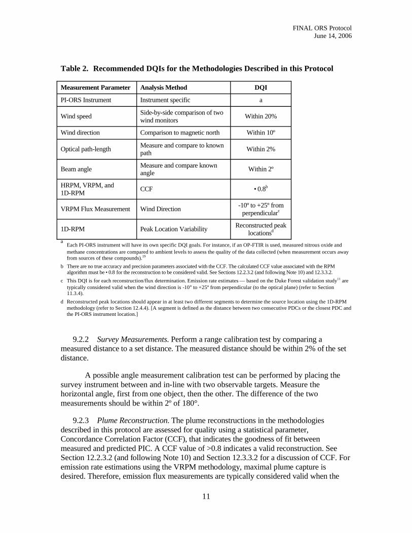
Table 2. Recommended DQIs for the Methodologies Described in this Protocol
Measurement Parameter Analysis Method DQI
PI-ORS Instrument Instrument specific a
Wind speed Side-by-side comparison of two wind monitors Within 20%
Wind direction Comparison to magnetic north Within 10º
Optical path-length Measure and compare to known path Within 2%
Beam angle Measure and compare known angle Within 2º
HRPM, VRPM, and 1D-RPM CCF •0.8b
VRPM Flux Measurement Wind Direction -10º to +25º from perpendicularc
1D-RPM Peak Location Variability Reconstructed peak locationsd
aEach PI-ORS instrument will have its own specific DQI goals. For instance, if an OP-FTIR is used, measured nitrous oxide and methane concentrations are compared to ambient levels to assess the quality of the data collected (when measurement occurs away from sources of these compounds).19
b There are no true accuracy and precision parameters associated with the CCF. The calculated CCF value associated with the RPM algorithm must be •0.8 for the reconstruction to be considered valid. See Sections 12.2.3.2 (and following Note 10) and 12.3.3.2.
c This DQI is for each reconstruction/flux determination. Emission rate estimates — based on the Duke Forest validation study11 are typically considered valid when the wind direction is -10° to +25º from perpendicular (to the optical plane) (refer to Section 11.3.4).
d Reconstructed peak locations should appear in at least two different segments to determine the source location using the 1D-RPM methodology (refer to Section 12.4.4). [A segment is defined as the distance between two consecutive PDCs or the closest PDC and the PI-ORS instrument location.]
9.2.2 Survey Measurements. Perform a range calibration test by comparing a measured distance to a set distance. The measured distance should be within 2% of the set distance.
A possible angle measurement calibration test can be performed by placing the survey instrument between and in-line with two observable targets. Measure the horizontal angle, first from one object, then the other. The difference of the two measurements should be within 2º of 180°.
9.2.3 Plume Reconstruction. The plume reconstructions in the methodologies described in this protocol are assessed for quality using a statistical parameter, Concordance Correlation Factor (CCF), that indicates the goodness of fit between measured and predicted PIC. A CCF value of >0.8 indicates a valid reconstruction. See Section 12.2.3.2 (and following Note 10) and Section 12.3.3.2 for a discussion of CCF. For emission rate estimations using the VRPM methodology, maximal plume capture is desired. Therefore, emission flux measurements are typically considered valid when the

FINAL ORS ProtocolJune 14, 2006
12
wind direction is close to perpendicular to the vertical plane (-10° to +25° for the Duke Forest validation study). Source locations using the 1D-RPM methodology are typically considered valid when the wind direction is within ±45º from perpendicular (to the line-of-sight). Reconstructed peak locations should appear in at least two different segments to determine the source location using the 1D-RPM methodology (refer to Section 12.4.4). A segment is defined as the distance between two consecutive PDCs or the closest PDC and the PI-ORS instrument location.
10.0 Calibration and Standardization
10.1 Instrument Calibration. The methodologies described in this protocol rely on accurate PIC data provided by a PI-ORS instrument. Calibration of these instruments isinstrument-specific and the user should refer to the instrument manual and EPA procedures for proper instrument calibration procedures.
10.2 Methodology Verification. The verification of the methodologies described in this protocol is a procedure to test the ability of each methodology to meet its objectives as described in Section 2.
10.2.1 Conduct a verification procedure involving a controlled gas release prior to using any new instrument/setup combination, and repeat the procedure when a significant change is made to any part of the PI-ORS instrument or setup. If only the methodology software is changed, a previously verified data set can be used for verification purposes. Detailed explanations of these peer-reviewed procedures using verification gases have been published for the HRPM,6 VRPM,7,9,11 and 1D-RPM 2,10 methodologies.
10.2.2 The verification procedure can be performed while data is collected in the fieldas long as the following three criteria are met: 1) the PI-ORS system is able to monitor more than one gas simultaneously; 2) the verification gas is one of these monitored gases; and 3) the verification gas is not emitted by the source under study. If these criteria are not met, this verification procedure must be performed in a separate location using the same setup geometry. Table 3 presents the DQI goals for the verification procedures.
10.3 HRPM Methodology – Verification Procedure. The verification procedure involves releasing gas from a defined area, simulating a hot spot.
10.3.1 A suggestion for simulating a hot spot is to release the verification gas through a soaker hose arranged in a star-shaped pattern. This simulated source should be situated in an arbitrary location within the measurement area and comparable in size to the dimensions of one pixel.
10.3.2 A set of twelve (12) cycles can be considered a complete verification procedure. A cycle is defined as one complete sequential data collection through all PDCs in the setup. Data acquisition (see Section 11.2.9) and analysis parameters for the verification procedure should be similar to those used for field measurements.

FINAL ORS ProtocolJune 14, 2006
13
Table 3. DQIs for Verification Procedures
Measurement Parameter Analysis Method Accuracy Precision % Completea
HRPM hot spot location Verification gas release 10% b NA 100%
VRPM emission rate estimation
Verification gas release 25%c NA 100%
1D-RPM upwind source location
Verification gas release 20%d NA 100%
a % Complete is the number of “valid” measurements (those that meet DQI goals for accuracy and precision) compared to the total number of measurements taken.
b The distance between the reconstructed peak concentration and the center of the simulated hot spot should be within 10 percent of the diagonal distance of the HRPM measurement area (see Section 10.2.3.3).
c The estimated release rate should be within ±25 percent of the measured (known) release rate to demonstrate an acceptable verification (see Section 10.2.4.5).
d The distance between the determined upwind source and the center of the simulated hot spot should be within 20 percent of the length of the 1D-RPM line-of-sight (see Section 10.2.5.3).
10.3.3 The software will reconstruct a surface concentration contour map for the HRPM configuration. The maximum concentration value of this map is considered the reconstructed peak concentration. The distance between the reconstructed peak concentration and the center of the simulated hot spot should be within 10 percent of the diagonal distance of the HRPM measurement area. This 10 percent criterion applies when 8 to 16 beams are used in the setup.
NOTE 7 - Fewer than 8 beams can be used in the HRPM configuration; however, a verification procedure is not needed due to the qualitative (low resolution) nature of the results.
10.4 VRPM Methodology - Verification Procedure. The verification procedure involves releasing gas from a defined area, simulating an area source.
10.4.1 A suggestion for simulating an area source is to release the verification gas through a soaker hose arranged in an “H”-shaped pattern. This simulated source should be situated almost immediately upwind from the VRPM plane. The distance between the VRPM plane and the nearest boundary of the simulated area source should be approximately five times the average height of the ground-level beam(s) (refer to Section 11.3). The dimensions of the simulated area source should be approximately one-third to one-half the length of the VRPM setup, and the “H” pattern should be centered with respect to the measurement plane.

FINAL ORS ProtocolJune 14, 2006
14
10.4.2 For the VRPM methodology verification procedure, the quantity of verification gas released over time should be measured. The precise starting and ending time of the release should be recorded.
10.4.3 The mass of the gas released can be determined in several ways. Two approaches are given below.
a) Weigh the gas cylinder prior to and after the release of the gas. Calculate the average actual emission rate of the gas. For example, if one kilogram (kg) of gas [1,000 grams (g)] is released over one hour [3,600 seconds (s)], the flux is calculated to be 1,000 g/3,600 s = 0.28 g/s.
b) Use a calibrated mass flowmeter to maintain a constant emission rate. The output emission rate from the mass flowmeter should be converted to units of g/s if necessary.
10.4.4 The software will calculate the flux of the verification gas through the VRPM plane. Fluxes should be averaged for all time periods when the measured wind direction is within -10° to + 25° from perpendicular to the vertical plane. These averaged values are considered valid as estimated emission rates for the verification procedure. A set of 12 cycles can be considered a complete verification procedure, as long as at least half of these cycles satisfy the -10° to + 25° from perpendicular wind criteria. Data acquisition (see Section 11.3.5) and analysis parameters for the verification procedure should be similar to those used for field measurements. It is recommended that at least 1 kg be released to minimize errors in weighing the cylinders.
10.4.5 Compare the measured emission rate value (Section 10.4.3) with the estimated emission rate from the VRPM methodology (Section 10.4.4). The calculated release should be ±25 percent of the measured release rate (known) to demonstrate an acceptable verification.
10.5 1D-RPM Methodology - Verification Procedure. The verification procedure involves releasing gas from a defined area, simulating a hot spot.
10.5.1 A suggestion for simulating a hot spot is to release the verification gas through a soaker hose arranged in a star-shaped pattern. This simulated source should be situated upwind from the 1D-RPM line-of-sight at a distance approximately equal to one-quarter of the length of the setup. This source should be centered with respect to the full length of the line-of-sight.
10.5.2 The software will determine the location of the upwind simulated source. The location should be determined using data collected during time periods when the measured wind direction is within ±45° from perpendicular to the 1D-RPM line-of-sight. A set of 12 cycles can be considered a complete verification procedure, as long as at least half of these cycles satisfy the ±45° from perpendicular wind criteria. Data acquisition (see Section

FINAL ORS ProtocolJune 14, 2006
15
11.4.4) and analysis parameters for the verification procedure should be similar to those used for field measurements.
10.5.3 The distance between the determined upwind source and the center of the simulated hot spot should be within 20 percent of the length of the 1D-RPM line-of-sight.
11.0 Procedure for Setup and Data Acquisition
11.1 Overview. High-quality PIC data are needed for input to the methodologies described in this protocol. A pre-study geographical site assessment should be conducted and an appropriate PI-ORS system must be selected. In addition, the user must choose the appropriate methodology – HRPM, VRPM, or 1D-RPM – depending on the purpose of the study.
11.1.1 The site assessment should collect information on the size, layout, and topography of the site, any physical barriers that may affect data collection, and the location of any possible off-site emission sources. This could include photographs and a detailed geographical site survey, which may be performed using a rangefinder, a theodolite, Geographical Positioning System (GPS), or similar instrument.
11.1.2 During the planning process, the seasonal prevailing wind direction expected during the time of the field campaign should be researched. This wind data, in conjunction with the suspected source location and site specific details, is used to design possible measurement setups.
11.2 HRPM Configuration. The HRPM configuration works best in an area without many topographical features, so that the PI-ORS beam paths are close to the ground. This enhances the ability to detect minor constituents emitted from the ground, since the emitted plumes may dilute significantly as they rise above ground level. Also, if the beam paths are elevated from the ground, the plume may drift underneath the nearest beam and be detected by a beam further away. This would result in a misrepresentation of the actual source location.
11.2.1 The PI-ORS instrument is typically placed at the origin (in the first quadrant of the Cartesian convention) of the rectangular area to be measured (see Figure 1). Special cases do arise when the scanner and the PI-ORS instruments are placed on the x-axis awayfrom the origin (see Note 3). For convenience, irregularly sized areas may be assumed to be rectangular. The maximum dimensions of the setup are limited only by the instrument-specific capabilities (i.e., maximum path length) and the user-required peak location resolution.
11.2.2 A survey instrument should be used to determine the length and width of the study area and the angle of the x-axis from magnetic north. The size of the sampling area and desired peak location resolution can be used to determine the optimal number of PDCs and their positions inside the area to be scanned.

FINAL ORS ProtocolJune 14, 2006
16
11.2.3 Once the HRPM measurement area and the number of PDCs have been determined, the area is divided into smaller rectangular areas called pixels. The total number of pixels required is smaller or equal to the total number of beam paths. The pixels are typically numbered in the order shown in Figure 1.
PI-ORS
Instrument
Flags
PDCs
PI-ORS
Instrument
Flags
PDCs
Flags
PDCs
Figure 1. Example of an HRPM Configuration Setup
11.2.4 In Figure 1, the survey area is divided into nine pixels of equal size. It should be noted that the survey area may be irregular in size, so that the resulting pixel grid is asymmetric (e.g., 2 by 4 pixels, 3 by 5 pixels, etc.). The total length of each axis should be divided by the number of pixels on that axis. This calculates the length of each pixel along each axis. Flags should be placed on each axis where each pixel boundary intersects (the location of the flags are indicated by the circles in Figure 1). These flags will be used as reference points for PDC placement.
NOTE 8 – Due to cost considerations associated with the PDCs, this protocol addresses HRPM setups utilizing a maximum of 16 PDCs. However, the use of a larger number of PDCs will increase the resolution of the peak location.
11.2.5 Figure 1 shows an example HRPM configuration setup. Each pixel will have at least one optical beam path that terminates within its boundaries at a PDC. This geometry maximizes the spread of the optical beams inside the area of emissions by passing one optical beam through the center of each pixel. The approximate location (in polar coordinates) of each PDC within each pixel is determined using trigonometric calculations.
11.2.6 Each PDC should be placed as close as possible to its calculated distance and angle from north. After all PDCs had been placed, a visual inspection should be made to ensure a clean line-of-sight to each PDC, and that each PDC is located within the appropriate pixel.
FINAL ORS ProtocolJune 14, 2006
17
11.2.6.1 A clean line-of-sight is ensured by looking at each PDC from the PI-ORS instrument. The PDC may need to be moved (within the appropriate pixel) to obtain a clear optical path.
11.2.6.2 The flags mentioned in Section 11.2.4 and illustrated in Figure 1 can be used as reference points for ensuring that each PDC is located within the boundaries of the appropriate pixel.
11.2.7 The optical beam is defined by the instrument and each PDC. Measure the actual pathlength and angle from magnetic north of each optical beam using a survey instrument.
11.2.8 It is recommended that a meteorological station is set up as part of the HRPM configuration. Although this data is not required for reconstructing the hot spot source location, wind speed and direction data may be helpful in interpreting the results.
11.2.9 Data Acquisition Parameters. Data acquisition parameters include total time of data collection and dwelling time per PDC. Data should be collected for a minimum of one hour during times when the wind meets the criteria defined in Section 4.2.2.3. Dwelling time per PDC is determined by 1) the specific project goals, and 2) the PI-ORS instrument-specific detection limits of the expected target gases. A recommended range for dwelling time per PDC is 10 to 60 seconds.
11.3 VRPM Configuration. The VRPM plane should be placed immediately downwind from the suspected emission source. The prevailing wind direction should be as perpendicular as possible to the vertical plane of measurement. The dimensions of the VRPM plane (length and height) should be maximized to capture as much of the plumeas possible.
11.3.1 The primary purpose of the VRPM methodology is to calculate the flux through the vertical plane. A minimum of two PDCs are necessary for this measurement – one of which should be on the ground defining the full length of the setup, and one on the vertical structure. The recommended setup for flux calculation is three PDCs, with one on the ground defining the full length of the setup, one at the top of the vertical structure, and one at approximately half of the height of the vertical structure.
NOTE 9 - Ground-level PDCs refer to those defining optical beams as close to horizontal as possible, given the topography of the site and the particular PI-ORS system characteristics.
11.3.2 In addition to measuring the flux, spatial information pertaining to the source homogeneity of the emitted plume can be obtained through the use of additional PDCs placed at intermediate lengths along the ground. This spatial information can be used to assess source homogeneity, and similar to the 1D-RPM methodology, can be used to determine the location of the upwind source (see Section 2.4.2). A minimum of four PDCs are necessary for the measurement of flux and plume spatial information, with three placed at ground level (one defining the full length of the setup) and one on the
FINAL ORS ProtocolJune 14, 2006
18
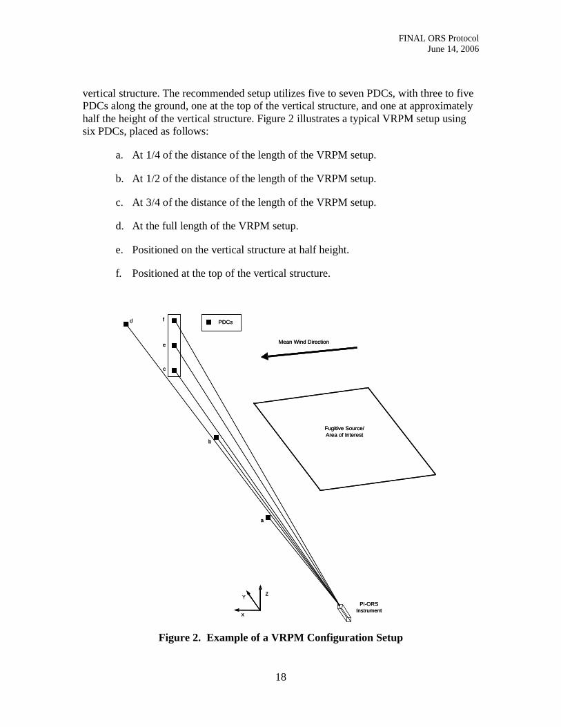
vertical structure. The recommended setup utilizes five to seven PDCs, with three to fivePDCs along the ground, one at the top of the vertical structure, and one at approximately half the height of the vertical structure. Figure 2 illustrates a typical VRPM setup using six PDCs, placed as follows:
a. At 1/4 of the distance of the length of the VRPM setup.
b. At 1/2 of the distance of the length of the VRPM setup.
c. At 3/4 of the distance of the length of the VRPM setup.
d. At the full length of the VRPM setup.
e. Positioned on the vertical structure at half height.
f. Positioned at the top of the vertical structure.
X
Y Z
PI-ORSInstrument
Fugitive Source/Area of Interest
Mean Wind Direction
PDCs
a
b
c
d
e
f
X
Y Z
PI-ORSInstrument
Fugitive Source/Area of Interest
Mean Wind Direction
PDCs
a
b
c
d
e
f
Figure 2. Example of a VRPM Configuration Setup
FINAL ORS ProtocolJune 14, 2006
19
11.3.3 The vertical structure should be located between the midpoint and far end of the VRPM setup, as referenced from the PI-ORS instrument (see Figure 2). Instrument-specific limitations and topography will dictate the specific placement of the vertical structure. For example, when collecting data under moderate to high wind conditions, it may be necessary to locate the vertical structure near the midpoint of the VRPM setup to optimize the PI-ORS instrument signal quality.
11.3.4 Prevailing Wind Direction Criteria. Ideally, the prevailing wind direction should be as close as possible to perpendicular to the VRPM measurement plane. This needs to be determined for each field study measurement configuration. For the Duke Forest validation study,11 the prevailing wind direction criteria was determined to be -10º to +25º, where 0º is perpendicular to the vertical plane. The procedure for determining theprevailing wind direction criteria is described in Appendix A (see Section A.2.3.2.4).
11.3.5 Data Acquisition Parameters. Data acquisition parameters include total time of data collection and dwelling time per PDC. Data collection should proceed regardless of the wind conditions (if safety permits) until a minimum of one hour of total data is collected during times when the wind meets the criteria defined in Sections 4.2.2.3 and 11.3.4. Dwelling time per PDC is determined by 1) the specific project goals, and 2) the PI-ORS instrument-specific detection limits of the expected target gases. A recommended range for dwelling time per PDC is 10 to 60 seconds.
11.3.6 Wind Measurements. The wind data should preferably be measured at two heights — near the base and near the top of the vertical plane (e.g., at 2 and 10 meters). Temporal resolution of the wind data should not be longer than the dwelling time on each PDC. The dual-height measurement of wind conditions allows for interpolation and extrapolation of this data through the vertical plane and is important in determining if the wind criteria have been met. In special cases when two wind monitors are not available, one wind monitor can be used at mid-height (3-5 m) to represent the average wind of the entire vertical plane.
11.3.7 When Data Acquisition and Wind Criteria Are Not Met. Data collection may proceed even when the one-hour data acquisition criterion is not met. Prior knowledge on source location and size, and actual wind direction, should be used to assess how much of the plume is captured by the setup. If the assessment of plume capture is valid (see Appendix A for a suggested method for plume capture assessment), the data can be used to estimate the emission rate. Without prior knowledge of source location and size, the data may be insufficient to estimate the emission rate.
11.4 1D-RPM Configuration. The 1D-RPM configuration is used to profile pollutant concentrations along a line-of-sight downwind of a fugitive emission source. This pollutant concentration profile can be combined with wind data to estimate the location of an upwind source, when applicable. The scanning PI-ORS instrument and three or more PDCs are placed along a crosswind direction and PIC measurements are made.
FINAL ORS ProtocolJune 14, 2006
20
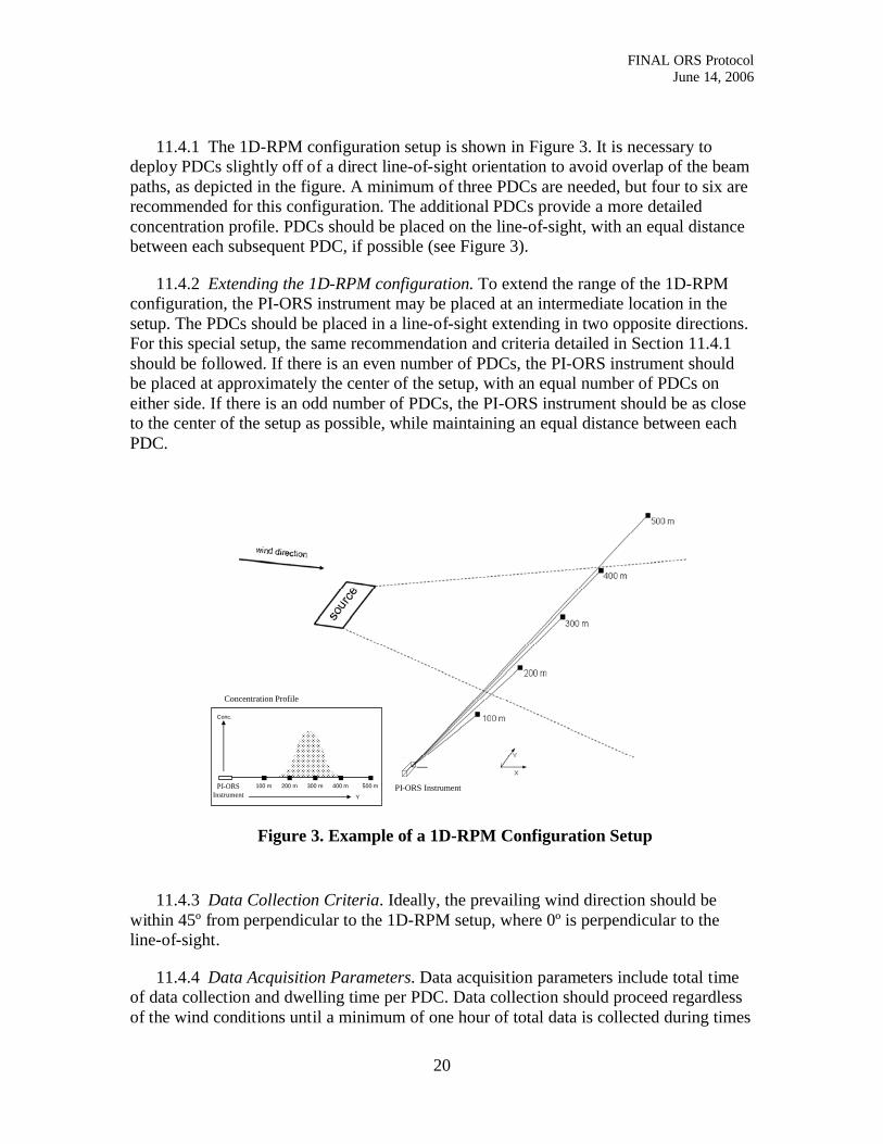
11.4.1 The 1D-RPM configuration setup is shown in Figure 3. It is necessary to deploy PDCs slightly off of a direct line-of-sight orientation to avoid overlap of the beam paths, as depicted in the figure. A minimum of three PDCs are needed, but four to six are recommended for this configuration. The additional PDCs provide a more detailed concentration profile. PDCs should be placed on the line-of-sight, with an equal distance between each subsequent PDC, if possible (see Figure 3).
11.4.2 Extending the 1D-RPM configuration. To extend the range of the 1D-RPM configuration, the PI-ORS instrument may be placed at an intermediate location in the setup. The PDCs should be placed in a line-of-sight extending in two opposite directions. For this special setup, the same recommendation and criteria detailed in Section 11.4.1 should be followed. If there is an even number of PDCs, the PI-ORS instrument should be placed at approximately the center of the setup, with an equal number of PDCs on either side. If there is an odd number of PDCs, the PI-ORS instrument should be as close to the center of the setup as possible, while maintaining an equal distance between each PDC.
Concentration Profile
PI-ORS InstrumentPI-ORS Instrument
100 m 200 m 300 m 400 m 500 m
Y
Conc.
Concentration Profile
PI-ORS InstrumentPI-ORS Instrument
100 m 200 m 300 m 400 m 500 m
Y
Conc.
Figure 3. Example of a 1D-RPM Configuration Setup
11.4.3 Data Collection Criteria. Ideally, the prevailing wind direction should be within 45º from perpendicular to the 1D-RPM setup, where 0º is perpendicular to the line-of-sight.
11.4.4 Data Acquisition Parameters. Data acquisition parameters include total time of data collection and dwelling time per PDC. Data collection should proceed regardless of the wind conditions until a minimum of one hour of total data is collected during times

FINAL ORS ProtocolJune 14, 2006
21
when the wind meets the criteria defined in Section 4.2.2.3 and 11.4.3. Dwelling time per PDC is determined by 1) the specific project goals, and 2) the PI-ORS instrument-specific detection limits of the expected target gases. A recommended range for dwelling time per PDC is 10 to 60 seconds.
11.4.5 Wind Measurements. The wind data should be measured in at least one location along the line-of-sight, with additional locations providing a better representation of the overall site wind field. Temporal resolution of the wind data should not be longer than the dwelling time on each PDC.
11.4.6 When Data Acquisition and Wind Criteria Are Not Met. Data collection may proceed even when the one-hour data acquisition criterion (within 45º from perpendicular) is not met. In this case, data should be collected for a total of two hours when the prevailing wind direction is within 70º from perpendicular to the 1D-RPM line-of-sight before reassessing the setup.
12.0 Data Analysis and Calculations
12.1 Overview. Prior to analysis, determine the moving averaging scheme for generation of the plume maps for any methodologies used in this protocol. Because data is acquired sequentially, a moving average is required to reduce errors that originate from temporal variability (see Appendix A, Section A2.3.2.2). Typically, a moving average with a grouping of three cycles is sufficient to provide stable results with a CCF larger than 0.8.
12.2 HRPM Methodology
12.2.1 HRPM Theory. Once the PIC for all beam paths are averaged with the predetermined grouping of cycles for the gas species of interest, the HRPM calculationsmake use of the information to reconstruct a plume map over the area of interest.
An example emission source location map is shown in Figure 4. The cross shows the location of the plume center from a study where propane gas was released at the location shown by the open circle.
12.2.2 HRPM Algorithm. Average concentrations for each pixel are obtained by applying an iterative algebraic deconvolution algorithm. The measured PIC, as a function of the field of concentration, is given by:
∑=m
mkmk cKPIC (12-1)

FINAL ORS ProtocolJune 14, 2006
22
Figure 4. An Example Emission Source Location Map
Where:
K = a kernel matrix that incorporates the specific beam geometry with the pixel dimensions;
k = the number index for the beam paths;
m = the number index for the pixels; and
c = the average concentration in the mth pixel.
12.2.2.1 Each value in the kernel matrix K is the length of the kth beam within the mth
pixel; therefore, the matrix is specific to the beam geometry. The HRPM procedure solves for the average concentrations (one for each pixel) by applying non-negative least squares (NNLS).23
12.2.2.2 The HRPM procedure multiplies the resulting vertical vector of averaged concentration by the matrix K to yield the end vector of predicted PIC data.
12.2.2.3 The second stage of the plume reconstruction involves interpolation among the reconstructed pixel’s average concentration, providing a peak concentration not limited to the center of the pixels. A triangle-based cubic interpolation procedure (in Cartesian coordinates) is currently used in the HRPM procedure.24
12.2.3 Check for Reasonableness of Surface Concentration Plot Results. Evaluate the data for reasonableness with the following qualitative (12.2.3.1) and quantitative (12.2.3.2) checks.

FINAL ORS ProtocolJune 14, 2006
23
12.2.3.1 If the order in which the beam paths were scanned (and the corresponding pixel numbering convention inside the HRPM program) are different than the order of PIC data input, the reconstructed plume center could fall in an incorrect pixel. Verify that the generated result is reasonable based on the raw PIC data.
12.2.3.2 To determine the quality of the reconstructed plume maps against the measured PIC data, the Concordance Correlation Factor (CCF) is used to represent the level of fit between measured PIC and predicted PIC. A CCF greater than 0.8 verifies that the surface concentration plot is a reasonable fit with the raw data (Table 2, Section 9.2).25 If the CCF is less than 0.8, the Check for Reasonableness procedures should be performed a second time to confirm the input data. The analysis may repeated with a longer average scheme, which typically increases the CCF value.
NOTE 10 — The CCF is similar to the Pearson correlation coefficient, but is adjusted to account for shifts in location and scale. Like the Pearson correlation (correlation coefficient, ‘R’), CCF values are bounded between -1 and 1, yet the CCF can never exceed the absolute value of the Pearson correlation factor. For example, the CCF will be equal to the Pearson correlation when the linear regression line intercepts the ordinate at 0, its slope equals 1. Its value will be lower than the Pearson correlation when the above conditions are not met.14,26 A detailed description of the procedure for calculating the CCF is included in Section 12.3.3.3.
12.2.4 Hot spot location determination The HRPM procedure provides a plume map and calculates the location of the peak concentrations. It is for the user to interpret this information and site constraints, such as obstructions or terrain complexities, for the determination of the actual location of the hot spot.
12.3 VRPM Methodology
12.3.1 VRPM Theory and Algorithms. Once the PIC for all beam paths are averaged with the predetermined grouping of cycles for the gas species of interest, the VRPM calculations make use of the information to reconstruct a plume map in the verticaldownwind plane. Two different beam configurations of the VRPM methodology are recommended: the five-beam (or more) and the three-beam VRPM configuration. Figure 2illustrates the setup for these two VRPM beam configurations. In the five-beam (or more) configuration, the ORS instrument sequentially scans over five PDCs. Three PDCs are along the ground-level crosswind direction (beams a, b, and c in Figure 2), and the other two are elevated on a vertical structure (beams e and f in Figure 2). The additional beam (d) in Figure 2 is for 6-beam configuration, which provides better spatial definition of the plume in the crosswind direction. In the three-beam configuration, the ORS instrument sequentially scans over three PDCs. Only one beam is along the ground level (beam c or d in Figure 2) and the other two are elevated on a vertical structure (beams e and f in Figure 2). PIC data are collected over time, completing many cycles through the defined beams of each configuration.
12.3.1.1 A two-phase smooth basis function minimization (SBFM) approach is applied where there are three or more beams along the ground level (5-beam or more

FINAL ORS ProtocolJune 14, 2006
24
configuration). In the two-phase SBFM approach, a one-dimensional SBFM reconstruction procedure is first applied in order to reconstruct the smoothed ground level and crosswind concentration profile. The reconstructed parameters are then substituted into the bivariate Gaussian function when applying a two-dimensional SBFM procedure.
12.3.1.1.1 A one-dimensional SBFM reconstruction is applied to the ground level segmented beam paths (Figure 2) of the same beam geometry to find the cross wind concentration profile. A univariate Gaussian function is fitted to measured PIC ground-level values.
12.3.1.1.2 The error function for the minimization procedure is the Sum of Squared Errors (SSE) function and is defined in the one-dimensional SBFM approach as follows:
2
0
2
21exp
2),,( ∑ ∑ ∫
−−−=
i j
r
jy
jy
jy
jijyjyj
i
drrmB
PICmBSSEσσπ
σ (12-2)
Where:
B = equal to the area under the one-dimensional Gaussian distribution (integrated concentration);
ri = the pathlength of the ith beam;
my = the mean (peak location);
σy = the standard deviation of the jth Gaussian function; and
PICi = the measured PIC value of the ith path.
12.3.1.1.3 The SSE function is minimized using the Simplex minimization procedure to solve for the unknown parameters (i.e., B, my, σy) .27
12.3.1.1.4 When there are more than three beams at the ground level, two Gaussian functions are fitted to retrieve skewed and sometimes bi-modal concentration profiles. This is the reason for the index j in Equation 12-2.
12.3.1.1.5 Once the one-dimensional phase is completed, the two-dimensional phase of the two-phase process is applied. To derive the bivariate Gaussian function used in the second phase, it is convenient to express the generic bivariate function G in polar coordinates r and θ:
( )( )( ) ( )G r A r m r m r m r m
y z
y
y
y z
y z
z
z
( , ) exp( cos ) cos sin sin
θπσ σ ρ ρ
θσ
ρ θ θ
σ σθσ
=−
−−
⋅ −−
⋅ − ⋅ −+
⋅ −
2 1
12 1
2
122
122
2
212
2
2(12-3)
FINAL ORS ProtocolJune 14, 2006
25
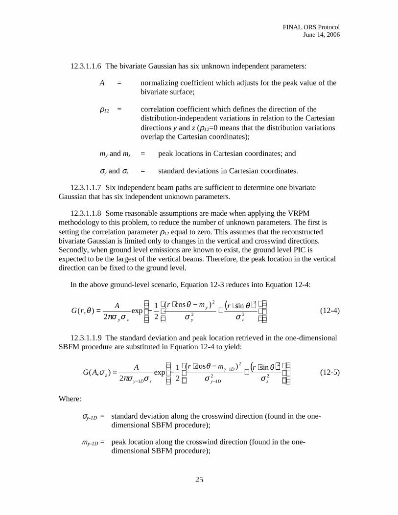
12.3.1.1.6 The bivariate Gaussian has six unknown independent parameters:
A = normalizing coefficient which adjusts for the peak value of the bivariate surface;
ρ12 = correlation coefficient which defines the direction of thedistribution-independent variations in relation to the Cartesian directions y and z (ρ12=0 means that the distribution variations overlap the Cartesian coordinates);
my and mz = peak locations in Cartesian coordinates; and
σy and σz = standard deviations in Cartesian coordinates.
12.3.1.1.7 Six independent beam paths are sufficient to determine one bivariate Gaussian that has six independent unknown parameters.
12.3.1.1.8 Some reasonable assumptions are made when applying the VRPM methodology to this problem, to reduce the number of unknown parameters. The first is setting the correlation parameter ρ12 equal to zero. This assumes that the reconstructed bivariate Gaussian is limited only to changes in the vertical and crosswind directions. Secondly, when ground level emissions are known to exist, the ground level PIC is expected to be the largest of the vertical beams. Therefore, the peak location in the vertical direction can be fixed to the ground level.
In the above ground-level scenario, Equation 12-3 reduces into Equation 12-4:
( )
⋅+
−⋅−= 2
2
2
2 sin)cos(21exp
2),(
zy
y
zy
rmrArGσ
θσ
θ
σπσθ (12-4)
12.3.1.1.9 The standard deviation and peak location retrieved in the one-dimensional SBFM procedure are substituted in Equation 12-4 to yield:
( )
⋅+
−⋅−=
−
−
−2
2
21
21
1
sin)cos(21exp
2),(
zDy
Dy
zDyz
rmrAAGσ
θσθ
σπσσ (12-5)
Where:
σy-1D = standard deviation along the crosswind direction (found in the one-dimensional SBFM procedure);
my-1D = peak location along the crosswind direction (found in the one-dimensional SBFM procedure);

FINAL ORS ProtocolJune 14, 2006
26
12.3.1.1.10 A and σz are unknown parameters to be retrieved in the second phase of the fitting procedure.
12.3.1.1.11 An error function (SSE) for minimization is defined for this phase in a similar manner. The SSE function for the second phase is defined as:
( ) ∑ ∫
−=
i
r
ziiiz
i
drArGPICASSE2
0
),,,(, σθσ (12-6)
Where:
PICi = the measured path-integrated concentration value of the ith path.
12.3.1.1.12 The SSE function is minimized using the Simplex method to solve for the two unknown parameters.
12.3.1.2 When the VRPM configuration consists only of three beam paths—one at the ground level and the other two elevated—the one-dimensional phase can be skipped, assuming that the plume is very wide. In this scenario, peak location can be arbitrarily assigned to be in the middle of the configuration. Therefore, the three-beam VRPM configuration is most suitable for area sources (where no localized hot spot is expected) or for sources with a series of point and fugitive sources that are known to be distributed across the upwind area. In this case, the bivariate Gaussian has the same two unknown parameters as in the second phase (Equations 12-5 and 12-6), but information about the plume width or location is not known. The standard deviation in the crosswind direction is typically assumed to be about 10 times that of the ground level beam path (length of vertical plane). If r1 represents the length of the vertical plane, the bivariate Gaussian would be as follows:
( )( )
⋅+
−⋅−= 2
2
21
212
1
1
sin10
)cos(21exp
)10(2),(
zzz
rr
rrr
AAGσ
θθσπ
σ (12-7)
This process is for determining the vertical gradient in concentration. It allows an accurate integration of concentrations across the vertical plane as the long-beam ground-level PIC provides a direct integration of concentration at the lowest level.
12.3.2 Once the parameters of the function are found for a specific run, the VRPM procedure calculates the concentration values for every square elementary unit in a vertical plane. Then, the VRPM procedure integrates the values, incorporating wind speed data at each height level to compute the flux. The concentration values are converted from parts per million by volume (ppmv) to grams per cubic meter (g/m3), taking into consideration the molecular weight of the target gas. This enables the direct calculation of the flux in grams per second (g/s), using wind speed data in meters per second (m/s).

FINAL ORS ProtocolJune 14, 2006
27
12.3.3 Check for Reasonableness of the Calculated Flux. Evaluate the data for reasonableness with the following qualitative (12.3.2.1) and quantitative (12.3.2.2) checks.
12.3.3.1 Verify that the generated result is reasonable based on the raw PIC data.12.3.3.2 To determine the quality of the reconstructed plume maps against the
measured PIC data, the CCF is used to represent the level of fit between measured PIC and predicted PIC (see Note 10).
12.3.3.3 As described in earlier studies,7 the Concordance Correlation Factor (CCF) was used to represent the level of fit for the reconstruction in the path-integrated domain (predicted versus measured PIC).
CCF is defined as the product of two components:
rACCF = (12-8)
Where:
r = the Pearson correlation coefficient;
A = a correction factor for the shift in population and location.
12.3.3.4 This shift is a function of the relationship between the averages and standard deviations of the measured and predicted PIC vectors:
12
21
−
−++=
MPP
M
M
P
PICPIC
MP
PIC
PIC
PIC
PIC PICPICAσσσ
σσσ
(12-9)
Where:
PPICσ = standard deviation of the predicted PIC vector;
MPICσ = standard deviation of the measured PIC vector;
PPIC = the mean of the predicted PIC vector; and
MPIC = the mean of the measured PIC vector.
12.3.3.5 The Pearson correlation coefficient is a good indicator of the quality of fit to the Gaussian mathematical function. In this procedure, typically an r close to 1 will be followed by an A very close to 1. This means that the averages and standard deviations in the two concentration vectors are very similar and the mass is conserved (good flux value). However, when a poor CCF is reported (CCF<0.80) at the end of the fitting

FINAL ORS ProtocolJune 14, 2006
28
procedure it does not directly mean that the mass is not conserved. It could be a case where only a poor fit to the Gaussian function occurred if the correction factor A was still very close to 1 (A>0.90). However, when both r and A are low one can assume that the flux calculation is inaccurate.
12.3.3.6 A CCF greater than 0.80 indicates that the surface concentration plot is a reasonable fit with the measured PIC (Table 2, Section 9.2).25 If the CCF is less than 0.80,but A>0.90, this is still a reasonable indication of a good mass equivalent surface concentration plot. If the CCF is less than 0.80, but A<0.90, then the Check for reasonableness procedures (Section 12.3.3) should be performed a second time to confirm the input data. The analysis may be repeated with a longer average scheme,which typically increases the CCF value.
12.4 1D-RPM Methodology
12.4.1 1D-RPM Theory and Algorithms. Once the PIC for all beam paths are averaged with the predetermined grouping of cycles for the gas species of interest, the1D-RPM calculations make use of the information to reconstruct a plume concentration profile along the measurement line-of-sight. Similar to the case of VRPM (which assumes a bivariate Gaussian plume mass in two dimensions), the 1D-RPM calculationsutilize the one-dimensional (1D) SBFM to reconstruct a mass-equivalent plume concentration profile along the line-of-sight measurement. The plume crosswind peak location, coupled with the average wind direction data, can provide an idea of the emission source location and configuration.
12.4.2 The 1D-RPM procedure fits a univariate Gaussian function to measured PIC ground-level values. The error function for the minimization procedure is the SSE function, and is defined in the 1D-SBFM approach as follows:
2
0
2
21exp
2),,( ∑ ∫∑
−−−=
i
r
y
y
j y
jiyyj
i
j
j
j
jjdr
rmBPICmBSSE
σσπσ (12-10)
12.4.3 The unknown independent parameters for the 1D-SPFM Gaussian are:
B = the area under the Gaussian distribution;
ri = the path length of the ith beam;
my = the mean (peak location);
σy = standard deviation of the jth Gaussian function; and
PICi = the measured path-integrated concentration value of the ith path.

FINAL ORS ProtocolJune 14, 2006
29
12.4.4 Check for Reasonableness of the Concentration Profile. Evaluate the data for reasonableness with the following qualitative (12.4.4.1) and quantitative (12.4.4.2) checks.
12.4.4.1 Verify that the generated result is reasonable based on the raw PIC data.
12.4.4.2 To determine the quality of the reconstructed plume maps against the measured PIC data, the CCF is used to represent the level of fit between measured PIC and predicted PIC (see Note 10). A CCF greater than 0.8 verifies that the surface concentration plot is a reasonable fit with the raw data (Table 2, Section 9.2).25 If the CCF is less than 0.8, the Check for Reasonableness procedures should be performed a secondtime to confirm the input data. The analysis may be repeated with a longer average scheme, which typically increases the CCF value.
NOTE 11 • The 1D-RPM methodology above explains a single Gaussian mass-equivalent plume. It is possible to fit multiple Gaussian plume profiles when more than three PDC are used [e.g., a combination of two Gaussian profiles with four or more PDC as explained in Hashmonay and Yost (1999)2]. This multiple Gaussian approach can provide multiple mode or skewed concentration profiles. Also this can be extended for VRPM configurations where four or more ground-level PDC are used to fit bi-modal or skewed bivariate Gaussian profiles. This may improve the accuracy of flux measurements, as it always provides higher CCF values.
12.4.5 The 1D-RPM procedure reconstructs the plume profile along the measurement line-of-site and notes the peak location. Over time, as the wind direction fluctuates, different peak locations are reconstructed from the PIC measurements as illustrated in Figure 5. Each time a peak location is noted, a source projection line is drawn for each peak location. This is done by calculating a line equation through the peak location, with the same orientation as the averaged wind direction for the same measurement time interval. Ideally, for a stationary point source, all source projection lines drawn over time should intersect at a point upwind of the measurement line in the vicinity of the real emission source location. Calculating the density of lines per unit area upwind from the measurement plane, the most likely location of the source can be estimated as the region of the maximal line density.
13.0 Methodology Performance
13.1 Data Quality Objectives. A verification gas release may be conducted during a field study to verify that the instrument is performing well, as long as the PI-ORS instrument is capable of detecting multiple compounds. Note the beginning and end of the release and the amount released.
13.1.1 For a verification gas release using the HRPM methodology, a plume center location error of ±10 percent of the diagonal distance of the entire area scanned is considered a good indicator of quality.

FINAL ORS ProtocolJune 14, 2006
30
13.1.2 For the weight of the verification gas release retrieved using the VRPM methodology, an error of ±25 percent of the total actual release for the duration of the experiment is considered a good indicator of quality.
13.1.3 For the location of the verification gas release using the 1D-RPM methodology, an error of ±20 percent of the longest beam path along the line-of-sight is considered a good indicator of quality.
Figure 5. An Example of a 1D-RPM Fenceline Monitoring Setup
14.0 Pollution Prevention
A discussion of pollution prevention issues is not necessary, as they are instrument specific and not directly associated with application of the methodologiesdescribed in this protocol.
Source Location
Reflectors
PI-ORSInstrument
Met Station
WindDirection
Industrial Complex
1 2 3
PDC

FINAL ORS ProtocolJune 14, 2006
31
15.0 Waste Management
Because no actual samples are collected with PI-ORS instrumentation, there are no waste management issues.
16.0 References1 Hashmonay, R. A.; Yost, M. G. Innovative Approach for Estimating Gaseous
Fugitive Fluxes Using Computed Tomography and Remote Optical Sensing Techniques. J. Air & Waste Manage. Assoc. 1999, 49, 966.
2 Hashmonay, Ram A.; Yost, Michael G. Localizing Gaseous Fugitive Emission Sources by Combining Real-Time Remote Optical Sensing and Wind Data. J. Air & Waste Manage. Assoc. 1999, 49, 1374-1379.
3 Hashmonay, R. A.; Yost, M. G.; Mamane, Y.; Benayahu, Y. Emission Rate Apportionment from Fugitive Sources Using Open-Path FTIR and Mathematical Inversion. Atmos. Environ. 1999, 33, 735-743.
4 Hashmonay, R. A.; Yost, M. G.; Wu, C. F. Computed Tomography of Air Pollutants Using Radial Scanning Path-Integrated Optical Remote Sensing. Atmos. Environ. 1999, 33(2), 267.
5 Price, P. N. Pollutant Tomography Using Integrated Concentration Data from Non-Intersecting Optical Paths. Atmos. Environ. 1999, 33(2), 275-280.
6 Wu, C. F.; Yost, M. G.; Hashmonay, R. A.; Park, D. Y. Experimental Evaluation of a Radial Beam Geometry for Mapping Air Pollutants Using Optical Remote Sensing and Computed Tomography. Atmos. Environ. 1999, 33(28), 4709-4716.
7 Hashmonay, R.A.; Natschke, D. F.; Wagoner, K.; Harris, D. B.; Thompson, E. L.; Yost, M. G. Field Evaluation of a Method for Estimating Gaseous Fluxes from Area Sources Using Open-Path Fourier Transform Infrared. Environ. Sci. Technol. 2001, 35, 2309-2313.
8 Yost, M. G.; Hashmonay, R. Mapping Air Contaminants Using Path-Integrated Optical Remote Sensing with a Non-Overlapping Variable Path Length Beam Geometry. U.S. Patent 6,542,242 B1, 2003.
9 Modrak, M. T.; Hashmonay, R. A.; Keagan [Kagann], R. Measurement of Fugitive Emissions at a Region I Landfill; U.S. Environmental Protection Agency, Research and Development, EPA-600/R-04-001, January 2004.
10 Thoma, E. D.; Shores, R. C.; Thompson, E. L.; Harris, D. B.; Thornloe, S. A.; Varma,R. M.; Hashmonay, R. A.; Modrak, M. T.; Natschke, D. F.; Gamble, H.A. Open

FINAL ORS ProtocolJune 14, 2006
32
Path Tunable Diode Laser Absorption Spectroscopy for Acquisition of Fugitive Emission Flux Data. J. Air & Waste Manage. Assoc. 2005, 55, 658-668.
11 Hashmonay, Ram A.; Varma, Ravi M.; Modrak, Mark T.; Kagann, Robert H.; Egler,Kim; Sullivan, Patrick D.; Segall, Robin R. Validation of Vertical Radial Plume Mapping Methodology for Estimating Gaseous Emission Rates from Area Sources. J. Air & Waste Manage. Assoc. Submitted in 2006.
12 Huang, Zhonghua; Wang, Junde; Li, Yan. Mapping Spacial Tracer Gases Concentration Profiles on a Two-Dimensional Plane by OP-FTIR Remote Sensing. Instrumentation Sci. & Technol. 2003, 31(1), 23-32.
13 Scotto, R. L.; Minnich, T. R.; Leo, M.R. A Method for Estimating VOC Emission Rates from Area Sources Using Remote Optical Sensing. In Proceedings of the EPA/A&WMA International Symposium on the Measurement of Toxic and Related Air Pollution, Raleigh, NC, 1991, 698.
14 Piccot, S. D.; Masemore, S. S.; Lewis-Bevan, W.; Ringler, E. S.; Harris, D. B. Field Assessment of a New Method for Estimating Emission Rates from Volume Sources Using Open-Path FTIR. J. Air & Waste Management Assoc. 1996, 46, 159.
15 Simpson, O. A.; Kagann, R. H. Measurements of Emissions at a Chemical Waste Water Site with an Open Path Remote Fourier Transform Interferometer. In Proceedings of the EPA/ A&WMA International Symposium on the Measurement of Toxic and Related Air Pollution, Raleigh, NC, 1990, 937.
16 Weber, Konradin; Lamp, Torsten; Schulte, Klaus;Weidemann, Johannes; van Haren,Günther; Gärtner, Andrea; Bröker, Günter. Open-Path FTIR-Measurements of Methane as a Tracer Gas for Waste Site Emissions at a Waste Site in Germany. Proceedings of the A&WMA 89th Annual Meeting & Exhibition, Pittsburgh, PA, 1996, 11p.
17 Heise,Michael; Müller, Uwe; Gärtner, Andrea; Hölscher; Norbert. Improved Chemometric Strategies for Quantitative FTIR Spectral Analysis and Applications in Atmospheric Open-Path Monitoring. Field Anal. Chem. & Technol. 2001, 5(1-2), 13-28.
18 Schäfer, Klaus; Steinecke, Ina; Emeis, Stefan; Stockhause, Martina; Sussmann, Ralf; Trickl, Thomas ; Reitebuch, Oliver; Hoechstetter, Karsten; Sedlmaier, Achim;Depta, Georg; Gronauer, Andreas; Seedorf, Jens; Hartung, Jörg. Inverse Modelling on the Basis of Remote Sensing to Determine Emission Rates. Meteorol. Zeitschrift, 1998, N.F. 7, 7-10 (Februar).
FINAL ORS ProtocolJune 14, 2006
33
19 Compendium Method TO-16: Long-Path Open-Path Fourier Transform Infrared Monitoring of Atmospheric Gases; U.S. Environmental Protection Agency,Center for Environmental Research Information-Office of Research and Development: Cincinnati, Ohio, January 1999.
20 American Society for Testing and Materials (ASTM) Standard Practice E1982-98, Standard Practice for Open-Path Fourier Transform Infrared (OP/FT-IR) Monitoring of Gases and Vapors in Air; March 1999.
21 American Society for Testing and Materials (ASTM) Standard Guide E1865-97 (Reapproved 2002), Standard Guide for Open-Path Fourier Transform Infrared (OP/FT-IR) Monitoring of Gases and Vapors in Air; July 1997.
22 VDI 4211, Part 1. Remote Sensing, Atmospheric Measurements Near Ground with FTIR Spectroscopy, Measurements of Gaseous Emissions and Immissions. Beuth Verlag Berlin, 2000.
23 Lawson, Charles L.; Janson, Richard J. Solving Least Squares Problems; Society for Industrial and Applied Mathematics: Philadelphia, 1995; Chapter 23, pp 158-165.
24 Barber, C. B., D.P. Dobkin, and H.T. Huhdanpaa, "The Quickhull Algorithm for Convex Hulls," ACM Transactions on Mathematical Software, Vol. 22, No. 4, Dec. 1996, p. 469-483.
25 Lin, L. I-K. A Concordance Correlation Coefficient to Evaluate Reproducibility.Biometrics. 1989, 45. 255-68.
26 Byer, R. L.; Shepp, L. A. Two-Dimensional Remote Air-Pollution Monitoring Via Tomography. Opt. Lett. 1979, 4(3), 75-77.
27 Press, W. H.; Teukolsky, S. A.; Vetterling, W. T.; Flannery, B.P. Numerical Recipes in FORTRAN, 2nd ed.; Cambridge University Press: Cambridge, MA, 1992.
FINAL DRAFT ORS ProtocolJune 14, 2006
34
Appendix A
Example Application of Methodologies Described in this Protocolusing OP-FTIR
The methodologies described in this protocol are independent of the particular PI-ORS instrument. This appendix has been included to illustrate the application of themethodologies described in this protocol during two separate experiments using a scanning open-path FTIR (OP-FTIR).A1-4 The methodologies described in this protocolhave been utilized for several other environmental monitoring programs.A5-7
A1.0 Examples of DQI Goals and Internal QC.
The Data Quality Indicator (DQI) goals for the OP-FTIR instrument are shown in Table A.1 The DQI goals were developed based on analysis of the historical data obtained in similar studies and available guidance documents.
Table A.1 Data Quality Indicators (DQIs) for OP-FTIR
Measurement Parameter Analysis Method Accuracy Precision % Complete
PIC Determination OP-FTIR: Nitrous Oxide Conc. ±25%/15%/10%a ± 10% 90%
Mid-IR absorbance OP-FTIR: Spectra Quality Acceptableb NA 100%
a The accuracy acceptance criterion is ±25 percent for pathlengths of less than 50 m, ±15 percent for pathlengths between 50 and 100 m, and ±10 percent for pathlengths greater than 100 m.
b Spectral quality must meet minimal quality (refer to instrumentation manuals and EPA methods for instrument-specific spectral quality criteria).
A1.1 Procedures for Evaluating OP-FTIR DQIs. The development and determination of DQIs for open-path measurements is an ongoing process. The following section detailsthe procedure for assessing the OP-FTIR DQI goals presented in Table A.1.
A1.1.1 PIC Determination. The accuracy and precision of the absorbance data may be verified by analyzing measured atmospheric nitrous oxide concentrations over time. This test is valid only if the background spectrum is void of nitrous oxide, and nitrous oxide is not used in the verification gas release. For the duration of the study, the calculated concentration results for nitrous oxide should be comparable to the natural ambient atmosphere level of 315 ppb ±25 percent for path lengths less than 50 meters, 315 ppb ±15percent for path lengths between 50 and 100 meters, and 315 ppb ±10 percent for pathlengths greater than 100.A8 Refer to Section 11.3.1.1 of ASTM Standard Practice E 1982-98 for more information on this procedure.A2
A1.1.2 Mid-IR Absorbance. The quality of the mid-IR absorbance data can be assessed by performing several qualitative and quantitative checks. These checks include assessing instrument noise, detector nonlinearity, detector saturation, and instrument
FINAL DRAFT ORS ProtocolJune 14, 2006
35
response. These checks were developed based on ASTM Standard Practice E 1982-98. Additional details on how to perform these checks can be found in the EPA documententitled, ECPB Optical Remote Sensing Facility Manual. A9
A1.2 Internal Quality Control. Traditional quality control (QC) samples are not applicable to OP-FTIR experiments. Instead, the analyses of IR-active ambient gases having relatively constant values are included in the quantification process. Examples include nitrous oxide and methane, which are found at relatively constant concentrations of 315 ppb and 1.7 ppm as global backgrounds, respectively. These must be used with caution, because a particular measurement area may prove to be a source of these gases. Methane, for example, is often emitted from hog waste lagoons and landfills.
A1.2.1 Generation of a Background Spectrum. As described in EPA Compendium Method TO-16 (1999),A2, A3 the generation of a background spectrum, more precisely the I0spectrum, is best accomplished synthetically. The best approach to this depends upon the software being used for processing the data. Many commercially available software systems are compatible with the data format used by OP-FTIR instruments. However, all of the available software options require analyst input; therefore, there is some subjectivity involved in the process.
A1.2.2 Data Integrity. Spectra are analyzed for peaks of common atmospheric constituents, such as water vapor, carbon dioxide, and methane. If these peaks are located outside of their expected spectral region or exhibit any other abnormal characteristics, a spectroscopist should manually examine a select portion of the original data to determine the reason for these deviations and/or the usability of the collected data.
A2.0 RPM Example using the HRPM and VRPM Methodologies
A2.1 Introduction. During the Fall of 2002 and Spring of 2003, the methodologies described in this protocol was evaluated using the controlled release of verification gases and a scanning monostatic OP-FTIR instrument. The experiments were performed at the Duke Forest Facility of Duke University, located in Chapel Hill, North Carolina. A nearly flat and square area of 14,400 m2 was selected for the study. The verification gases released during the experiments included ethylene and acetylene. This example briefly describes the preliminary results obtained from this controlled demonstration study using the HRPM and VRPM methodologies.
A2.2 Experimental Setup. This study was supported by the Environmental Security Technology Certification Program (ESTCP) of the Department of Defense (DoD) and audited by the Emissions Monitoring Center (EMC) of the EPA.
In this study, an OP-FTIR mounted on a scanner and an array of mirrors (PDC) formed multiple, non-intercepting beam paths. Nine mirrors were used for the HRPM experiment, and five were used for the VRPM experiment. The OP-FTIR was scanned sequentially from mirror to mirror, acquiring spectra from each beam path. The OP-FTIR

FINAL DRAFT ORS ProtocolJune 14, 2006
36
dwelling time on each mirror was 30 seconds for the HRPM experiment and 60 seconds for the VRPM experiment.
A2.3 Results and Discussion. PIC data were derived from the collected spectra, and wind data were time-synchronized with the spectral data and averaged for the corresponding measurement cycle. Following this, the PIC data were sorted according to mirror number, and the expanded data matrix (see Table A.2) was then used as input to the software developed by ARCADIS in Research Triangle Park, NC. In the case of the HRPM methodology, the software reconstructs the surface concentration contour map. In the case of the VRPM methodology, the software provides spatial information on the homogeneity of the plume, and calculates the emission flux through the configuration.
A2.3.1 HRPM Results. Several verification gases were released at random locations and spectral data were collected by sequentially scanning the OP-FTIR from mirror to mirror. This spectral data were used to derive PIC data along each beam path, which were then input into the RPM software to construct a surface concentration contour map. The hot spot location was determined by the area of highest concentrations in the contour map. Thislocation was then compared to the actual release location of the verification gas.
For this example, acetylene was released and data were collected for 18 cycles. Figure A.1 shows the concentration contour map constructed by averaging PIC data fromall 18 cycles. The open circle indicates the actual release location, and the closed circle indicates the hot spot location determined by the software. The dislocation distance (distance between the actual and determined release location) is shown with a double-headed arrow. In this case, the dislocation distance was 17 meters. Table A.2 presents the data matrix used to construct Figure A.1.

FINAL DRAFT ORS ProtocolJune 14, 2006
37
Figure A.1 Actual Versus Determined Source Location for the Acetylene Release
Table A.2 Data Matrix Used to Construct Figure A.1Pixel no. 1 2 3 4 5 6 7 8 9
Physical Beam Path Length (m) 68.4 102.6 148.9 103.1 137.2 169.6 149.1 171.2 178.5
Cycle 1 (ppm-m) 0.0 0.0 0.0 0.0 0.0 0.0 11.6 23.2 0.0Cycle 2 (ppm-m) 0.0 1.3 0.0 0.0 0.0 0.0 0.0 32.6 0.0Cycle 3 (ppm-m) 0.0 0.0 0.0 0.0 0.0 0.0 0.0 5.2 0.0Cycle 4 (ppm-m) 0.0 1.1 0.0 0.0 0.0 0.0 8.5 6.6 0.0Cycle 5 (ppm-m) 1.0 1.0 0.0 0.0 0.0 2.3 49.6 34.3 0.0Cycle 6 (ppm-m) 0.0 0.0 0.0 0.0 0.0 2.1 6.5 7.5 0.0Cycle 7 (ppm-m) 0.0 0.0 0.0 0.0 1.4 0.0 8.0 11.7 0.0Cycle 8 (ppm-m) 0.0 0.0 0.0 4.0 0.0 0.0 55.6 62.8 1.8Cycle 9 (ppm-m) 0.0 0.0 0.0 0.0 0.0 0.0 8.2 4.2 0.0
Cycle 10 (ppm-m) 1.1 0.5 0.0 0.0 1.1 0.0 8.0 73.0 0.0Cycle 11 (ppm-m) 0.0 0.0 0.0 0.0 0.0 0.0 28.3 0.0 0.0Cycle 12 (ppm-m) 0.0 0.0 0.0 0.0 0.0 0.0 28.8 91.9 0.0Cycle 13 (ppm-m) 0.0 0.0 0.0 0.0 0.0 2.4 49.1 10.1 3.2Cycle 14 (ppm-m) 0.0 0.0 0.0 0.0 0.0 4.4 25.5 119.1 2.1Cycle 15 (ppm-m) 0.8 0.0 1.3 0.0 0.0 1.9 63.0 192.0 2.8Cycle 16 (ppm-m) 0.0 0.0 0.0 4.1 0.0 2.7 78.0 12.4 0.0Cycle 17 (ppm-m) 1.1 1.0 0.0 49.6 0.0 0.0 303.0 247.2 0.0Cycle 18 (ppm-m) 37.9 0.0 0.0 120.7 52.4 13.4 169.1 199.6 98.7
18-Cycle Average (ppm-m) 2.33 0.27 0.07 9.91 3.05 1.62 50.04 62.97 6.03

FINAL DRAFT ORS ProtocolJune 14, 2006
38
A2.3.2 VRPM Results. Several verification gases were released in an “H” pattern upwind of the VRPM configuration to simulate a small area source in Duke Forest (see Figure A.2).A9 The verification gas cylinders were weighed before and after each release to calculate the actual release rate (in g/s). Spectral data were collected by sequentially scanning the OP-FTIR from mirror to mirror. This data were used to derive PIC data along each beam path, which were used as input to the VRPM algorithm to determine a plane-integrated concentration. Wind data were simultaneously collected at two heights (2 and 10 m), and were incorporated with the plane-integrated concentration data to calculate the emission flux through the VRPM configuration.
Figure A.2 Schematic of the VRPM Configuration Used for the Ethylene Release
For this example, ethylene was released and data were collected for 12 cycles. Figure A.3 shows the reconstructed mass-equivalent plume map constructed by averaging PIC data from all 12 cycles. A total of 1.0 lb of ethylene was released over a period of 68 minutes, which resulted in an average release rate of 0.11 g/s. The average calculated emission flux was 0.10 g/s. Table A.3 presents the data matrix used to construct Figure A.3.
X
Y Z
15 m30 m
30 m
90 m
40 m
50 m
90 m
140 m
7 m
13 m
Scanning OP-FTIR
Mean Wind Direction
Retroreflectors

FINAL DRAFT ORS ProtocolJune 14, 2006
39
Figure A.3 Flux Measurement for Ethylene
Table A.3 Data Matrix Used to Construct Figure A.3
Beam Path no. 1 2 3 4 5Physical Beam Path Length (m) 52.1 90.1 137 141.5 141.9
WS (m/s)
WD from Normal(deg)
Cycle 1 (ppm-m) 2.7 13.4 17.8 3.8 5.1 2.7 5Cycle 2 (ppm-m) 6.4 28.0 19.4 9.0 5.4 2.6 1Cycle 3 (ppm-m) 4.5 23.4 23.1 8.8 7.9 2.1 0Cycle 4 (ppm-m) 2.8 28.3 20.4 10.0 7.3 2.1 14Cycle 5 (ppm-m) 5.0 19.8 34.7 4.2 5.3 2.9 13Cycle 6 (ppm-m) 2.9 27.9 14.4 11.1 7.8 2.9 3Cycle 7 (ppm-m) 10.8 14.1 28.5 4.7 7.9 3.0 -11Cycle 8 (ppm-m) 2.7 10.3 49.1 4.9 5.8 2.3 18Cycle 9 (ppm-m) 2.7 23.1 25.8 23.3 7.1 1.8 -2Cycle 10 (ppm-m) 6.7 11.6 18.7 4.5 11.1 1.7 -15Cycle 11 (ppm-m) 14.4 20.2 36.0 15.7 7.0 2.0 -8Cycle 12 (ppm-m) 2.6 3.3 30.9 8.3 6.7 2.2 14
12-Cycle Average (ppm-m) 5.4 18.6 26.6 9.0 7.0 2.35 3
BOLD values represent one-half the minimum detection limit.
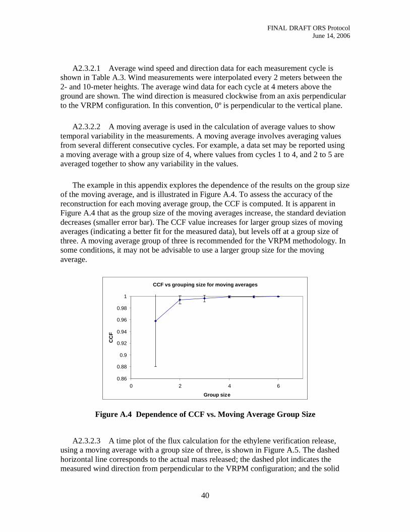
FINAL DRAFT ORS ProtocolJune 14, 2006
40
A2.3.2.1 Average wind speed and direction data for each measurement cycle is shown in Table A.3. Wind measurements were interpolated every 2 meters between the 2- and 10-meter heights. The average wind data for each cycle at 4 meters above the ground are shown. The wind direction is measured clockwise from an axis perpendicular to the VRPM configuration. In this convention, 0º is perpendicular to the vertical plane.
A2.3.2.2 A moving average is used in the calculation of average values to show temporal variability in the measurements. A moving average involves averaging values from several different consecutive cycles. For example, a data set may be reported using a moving average with a group size of 4, where values from cycles 1 to 4, and 2 to 5 are averaged together to show any variability in the values.
The example in this appendix explores the dependence of the results on the group size of the moving average, and is illustrated in Figure A.4. To assess the accuracy of the reconstruction for each moving average group, the CCF is computed. It is apparent in Figure A.4 that as the group size of the moving averages increase, the standard deviation decreases (smaller error bar). The CCF value increases for larger group sizes of moving averages (indicating a better fit for the measured data), but levels off at a group size of three. A moving average group of three is recommended for the VRPM methodology. In some conditions, it may not be advisable to use a larger group size for the moving average.
CCF vs grouping size for moving averages
0.86
0.88
0.9
0.92
0.94
0.96
0.98
1
0 2 4 6
Group size
CC
F
Figure A.4 Dependence of CCF vs. Moving Average Group Size
A2.3.2.3 A time plot of the flux calculation for the ethylene verification release, using a moving average with a group size of three, is shown in Figure A.5. The dashedhorizontal line corresponds to the actual mass released; the dashed plot indicates the measured wind direction from perpendicular to the VRPM configuration; and the solid
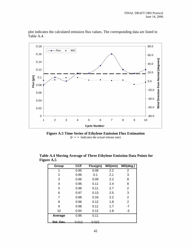
FINAL DRAFT ORS ProtocolJune 14, 2006
41
plot indicates the calculated emission flux values. The corresponding data are listed in Table A.4.
0
0.02
0.04
0.06
0.08
0.1
0.12
0.14
0.16
0.18
1 2 3 4 5 6 7 8 9 10
Cycle Number
Flux
[g/s
]
-80.0
-60.0
-40.0
-20.0
0.0
20.0
40.0
60.0
80.0
Win
d D
irect
ion
from
Nor
mal
[deg
rees
]
Flux WD
Figure A.5 Time Series of Ethylene Emission Flux Estimation(• • • Indicates the actual release rate)
Table A.4 Moving Average of Three Ethylene Emission Data Points for Figure A.5
Group CCF Flux(g/s) WS(m/s) WD(deg.)1 0.95 0.08 2.2 22 0.96 0.1 2.1 33 0.96 0.09 2.2 84 0.96 0.11 2.4 85 0.96 0.11 2.7 26 0.97 0.13 2.5 37 0.98 0.16 2.2 28 0.96 0.12 1.8 29 0.98 0.11 1.7 -7
10 0.94 0.12 1.8 -3Average 0.96 0.11
Std. Dev. 0.012 0.022
FINAL DRAFT ORS ProtocolJune 14, 2006
42
A2.3.2.4 The example below of flux data from the Duke Forest study provides guidance for determining the range of wind directions that will ensure complete capture of the plume (in the horizontal direction) by the VRPM configuration. The VRPM flux results are representative of the source emission rate only during periods that the prevailing wind directions meet the established criterion.
The determination of the acceptable wind criterion is done by analyzing a data set of calculated flux values, with the corresponding wind direction, at the time of the flux calculation. The data set should consist of data collected over a wide range of wind directions on both sides of the perpendicular direction to the VRPM configuration. A plot is create of the calculated flux values as a function of the angle of the prevailing wind direction (from perpendicular to the VRPM configuration) of all runs made when the wind direction angles were close to the perpendicular direction of the VRPM configuration. Because these runs were collected over a period of six months, the flux values were normalized to the maximum flux value in each run.
Figure A.6 presents a plot of this data set. The figure shows the calculated normalized flux values and the corresponding wind direction (from the normal to the VRPM configuration during the time of the measurements).
The figure shows that the raw flux values steadily increase, up to a certain point, as the prevailing wind direction becomes closer to perpendicular to the configuration. However, over a certain range of wind directions, there appears to be no relationship between calculated flux values and prevailing wind direction. This range is approximately between -10° and +25° for the Duke Forest validation study. This is the approximate range of acceptable wind directions, as the variations in flux values in this range are due to variations in the source strength, and not due to changes in wind direction. It is recommended that these flux plots be smoothed out with a moving average approach to retrieve a more definite and accurate cutoff of the wind criterion. The lined curves in the figure show examples of such moving averages, one with a grouping of 10 data values (thin line) and the other with a grouping of 20 data values (thicker line). These examples of moving averages clearly define the range of wind directions where flux values are independent from the wind direction values.
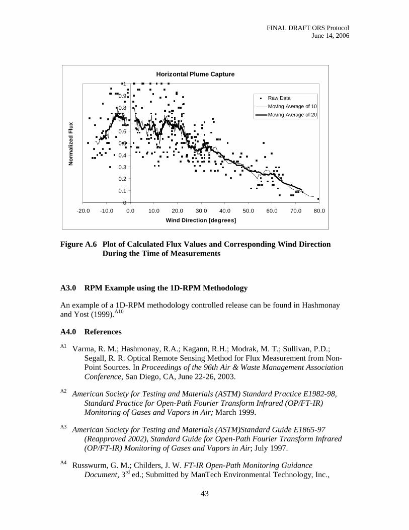
FINAL DRAFT ORS ProtocolJune 14, 2006
43
Horizontal Plume Capture
0
0.1
0.2
0.3
0.4
0.5
0.6
0.7
0.8
0.9
1
-20.0 -10.0 0.0 10.0 20.0 30.0 40.0 50.0 60.0 70.0 80.0
Wind Direction [degrees]
Nor
mal
ized
Flu
x
Raw DataMoving Average of 10Moving Average of 20
Figure A.6 Plot of Calculated Flux Values and Corresponding Wind Direction During the Time of Measurements
A3.0 RPM Example using the 1D-RPM Methodology
An example of a 1D-RPM methodology controlled release can be found in Hashmonay and Yost (1999).A10
A4.0 ReferencesA1 Varma, R. M.; Hashmonay, R.A.; Kagann, R.H.; Modrak, M. T.; Sullivan, P.D.;
Segall, R. R. Optical Remote Sensing Method for Flux Measurement from Non-Point Sources. In Proceedings of the 96th Air & Waste Management Association Conference, San Diego, CA, June 22-26, 2003.
A2 American Society for Testing and Materials (ASTM) Standard Practice E1982-98, Standard Practice for Open-Path Fourier Transform Infrared (OP/FT-IR) Monitoring of Gases and Vapors in Air; March 1999.
A3 American Society for Testing and Materials (ASTM)Standard Guide E1865-97 (Reapproved 2002), Standard Guide for Open-Path Fourier Transform Infrared (OP/FT-IR) Monitoring of Gases and Vapors in Air; July 1997.
A4 Russwurm, G. M.; Childers, J. W. FT-IR Open-Path Monitoring Guidance Document, 3rd ed.; Submitted by ManTech Environmental Technology, Inc.,
FINAL DRAFT ORS ProtocolJune 14, 2006
44
under contract 68-D5-0049 to the U.S. Environmental Protection Agency, Human Exposure and Atmospheric Sciences Division, National Exposure Research Laboratory: Research Triangle Park, NC, 1999.
A5 Modrak, M. T.; Hashmonay, R. A.; Keagan [Kagann], R. Measurement of Fugitive Emissions at a Region I Landfill; U.S. Environmental Protection Agency, Research and Development, EPA-600/R-04-001, January 2004.
A6 Hashmonay, R.A.; Natschke, D. F.; Wagoner, K.; Harris, D. B.; Thompson, E. L., Yost, M. G. Field Evaluation of a Method for Estimating Gaseous Fluxes from Area Sources Using Open-Path Fourier Transform Infrared. Environ. Sci. Technol. 2001, 35, 2309-2313.
A7 Modrak, M. T.; Varma, R. M.; Hashmonay, R. A.; Kagann, R. H.; Bolch, M. A.Demonstration of Optical Remote Sensing Method for Flux Measurement from Non-Point Sources. In Proceedings of the 97th Air & Waste Management Association Conference, Indianapolis, IN, June 22-25, 2004.
A8 ARCADIS G&M, Inc. ECPB Optical Remote Sensing Facility Manual; U.S. Environmental Protection Agency, Emissions Characterization and Prevention Branch, Research Triangle Park, NC; Contract No. EP-C-04-023, Work Assignment No. 0-33, expected publication 2006.
A9 Hashmonay, Ram A.; Varma, Ravi M.; Modrak, Mark T.; Kagann, Robert H.; Egler, Kim; Sullivan, Patrick D.; Segall, Robin R. Validation of Vertical Radial Plume Mapping Methodology for Estimating Gaseous Emission Rates from Area Sources. J. Air & Waste Manage. Assoc. Submitted in 2006.
A10 Hashmonay, Ram A.; Yost, Michael G. Localizing Gaseous Fugitive Emission Sources by Combining Real-Time Remote Optical Sensing and Wind Data. J. Air & Waste Manage. Assoc. 1999, 49, 1374-1379.