1

SBPG programme

December 2010

Optical microscopy basics

Advanced Technology Development Group

B. VojnovicGray Institute for Radiation Oncology and Biology, Oxford

The Randall Centre, King’s College, London

boris.vojnovic@rob.ox.ac.uk

2

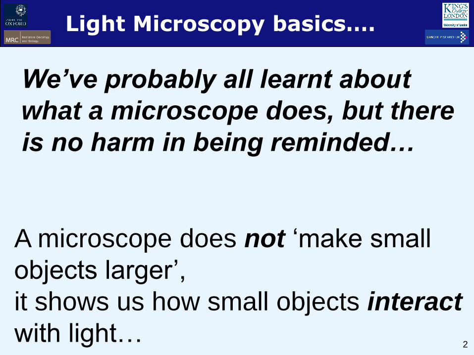
Light Microscopy basics….

We’ve probably all learnt about

what a microscope does, but there

is no harm in being reminded…

A microscope does not ‘make small

objects larger’,

it shows us how small objects interact

with light…

3

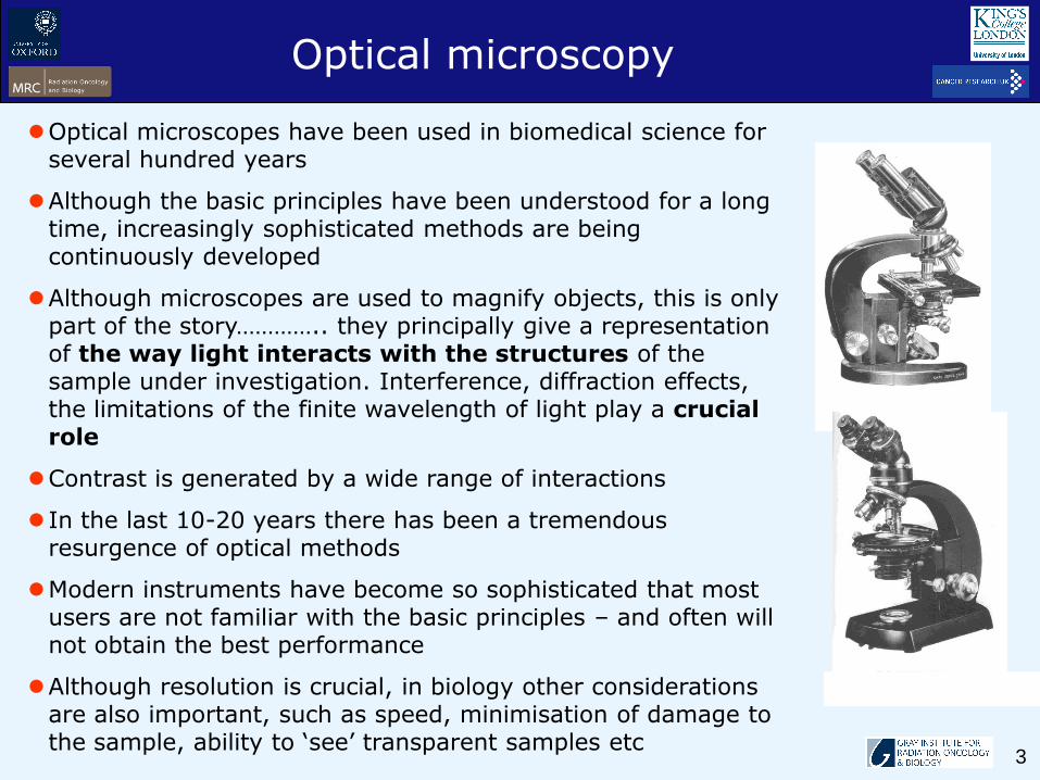
Optical microscopy

Optical microscopes have been used in biomedical science for several hundred years

Although the basic principles have been understood for a long time, increasingly sophisticated methods are being continuously developed

Although microscopes are used to magnify objects, this is only part of the story………….. they principally give a representation of the way light interacts with the structures of the sample under investigation. Interference, diffraction effects, the limitations of the finite wavelength of light play a crucial role

Contrast is generated by a wide range of interactions

In the last 10-20 years there has been a tremendous resurgence of optical methods

Modern instruments have become so sophisticated that most users are not familiar with the basic principles – and often will not obtain the best performance

Although resolution is crucial, in biology other considerations are also important, such as speed, minimisation of damage to the sample, ability to ‘see’ transparent samples etc

4

5

Particles and energies

Electron volt = 1.602 176 462 x 10-19 Joules

Electron mass = 9.10938215(45) × 10−31 kg

Elementary charge = 1.602 176 462 x 10-19 Coulombs

Photon = zero mass and zero electric charge

100 nm 3 x 1015 Hz 12.4 eV200 nm 1.5 x 1015 Hz 6.20 eV500 nm 6 x 1014 Hz 2.48 eV1000 nm 3 x 1014 Hz 1.24 eV

E = h = h c/

Energy

Planck’s constant

frequency

Speed of light

wavelength

Planck’s constant = 6.626 068 76 x 10-34 Joule seconds

6

Where it all started….

Antonie van Leeuwenhoek

(1632-1723)

Ball lens (=shortest focal length) microscope

Van Leeuwenhoek maintained throughout his life that there were aspects of microscope construction "which I only keep for myself", including in particular his most critical secret: how did he create the lens……

Not much has changed!.....try obtaining a lens prescription from Zeiss, Nikon, others…..

7

Microscopes can be beautiful…

From http://www.antique-microscopes.com/

8

http://micro.magnet.fsu.eduAn excellent web site

Where to learn all about microscopy….

Also: https://support.svi.nl/wiki/index.php

9

Lens basics

u v

ff

V

U

u v f

1 1 1+ =

V v U u

=

Biconvex Plano-convex

Positive meniscus

Negative meniscus

Plano-concave

Biconcave

8 f

Point object at infinite

distance

Lens forms using

spherical surfaces

10

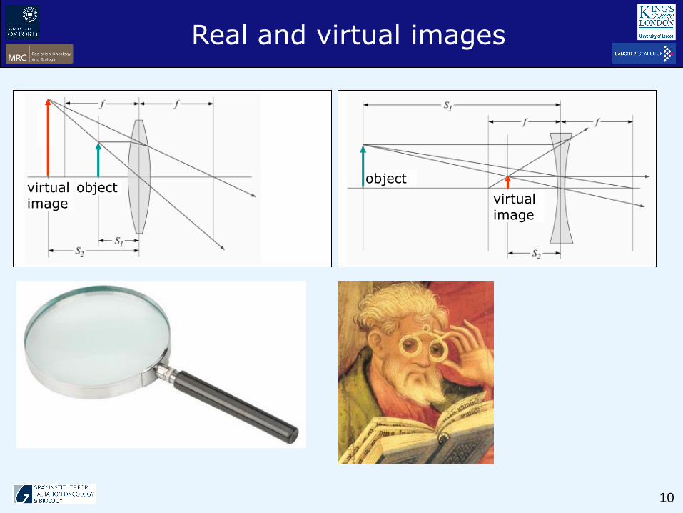
Real and virtual images

object

virtual image

objectvirtual image

11

Spherical aberration

Coma

image

Lens aberrations

Parallel rays (from object at infinity) do not converge to a single point (focus)

Aberrations reduced by utilising smaller portion of lens input area: aperture reduction

12

Chromatic aberration

Achromatic doublet

Crown glass

Flint glass

Astigmatism

on-axis

off-axis

Lens aberrations

13

Compound lenses

Multiple elements used to correct for individual aberrations: examples of astigmats and achromatic astigmats

14

Wave diffraction

Google earth:Panama canal entrance

Francesco Grimaldi coined the term diffraction (Latin diffringere, 'to break into pieces‘)Thomas Young, Augustin-Jean Fresnel, Christiaan Huygens, Joseph von Fraunhofer

15

The ability of an imaging system to resolve detail is ultimately limited by diffraction

A plane wave incident on a circular lens (or spherical mirror) is diffracted

Light is not focused to a point but forms an Airy disk having a central spot in the focal plane with radius to first null of:

where λ is the wavelength of the light and N is the f-number (focal

length divided by diameter) of the imaging optics.

In object space, the corresponding angular resolution is:

Diffraction

D is the diameter of the entrance pupil of the imaging lens

16

objective

first objective lens

= 30o

NA = n sin()

NA = 0.5 NA = 0.75

= 48.7o

NA = 0.95

= 72.1o

n = refractive index (air=1, water = 1.3, oil =1.4)

Numerical aperture

Resolution = 1.22 / 2NA

Resolution = 1.22 / NA objective + NA condenser

= half-angle of light cone collected

17

half-angle subtended and

% collected; air objective

0

10

20

30

40

50

60

0 0.2 0.4 0.6 0.8 1

numerical aperture

an

gle

(d

eg

) o

r p

erc

en

tag

e

θ/2

% collected

Objective numerical aperture

0.3 na 660 nm 1.342 m

Resolution = 1.22 / 2NA

500 nm

450 nm

1.021 m

0.813 m

0.75 na 660 nm 0.537 m

500 nm

450 nm

0.408 m

0.325 m

18

Objects in the optical microscope that are either self-luminous or illuminated by a large-angle cone of light form Airy patterns at the intermediate image plane that are incoherent and do not interfere with each other

This allows the determination of the minimum separation distance between adjacent Airy patterns by examination of the total intensity distribution (the sum of intensities) when these patterns are closely spaced or overlapping

When the separation distance between adjacent Airy patterns is greater than the central disc radius, the sum of the intensities yields two individual peaks. As the discs approach each other, the separation distance will reach a value equal to the central disc radius, a condition known as the Rayleigh criterion

At even closer approach, the separation distance is less than the central disc radius and the sum of the two peaks merges into a single peak. In the latter instance, the two Airy patterns are said not to be resolved

Microscope resolution

19

Airy pattern from point sources

Amplitude (EM field)

Intensity (brightness)

Airy disc

20

Köhler illumination –parfocality in a microscope

21

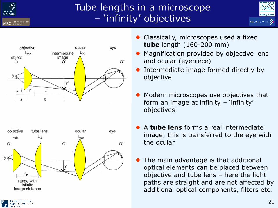
Classically, microscopes used a fixed tube length (160-200 mm)

Magnification provided by objective lens and ocular (eyepiece)

Intermediate image formed directly by objective

Modern microscopes use objectives that form an image at infinity – ‘infinity’ objectives

A tube lens forms a real intermediate image; this is transferred to the eye with the ocular

The main advantage is that additional optical elements can be placed between objective and tube lens – here the light paths are straight and are not affected by additional optical components, filters etc.

Tube lengths in a microscope – ‘infinity’ objectives

22IMAGING LIGHT PATHS ILLUMINATION LIGHT PATHS

Eye

Eyepiece

Intermediate

image plane

Object

Condenser

.

Collector Lens

Lamp

Objective Objective back focal plane

Tube

lens

Light paths in

transmitted-light

microscope using

Köhler illumination

Condenser diaphragm - determines

condenser numerical aperture

Field diaphragm - determines

illuminated sample area

23

Johann Ploem

(1927 -

Georges Nomarski

(1919 - 1997)

Frits Zernike

(1888-1966)

Phase Contrast

microscopy

Robert Day Allen

(1927-1986)

Fluorescence

microscopy

Differential

Interference

Contrast

Video microscopy

Ernst Abbe

(1840-1905)

Microscopy developments in modern times

24

Microscope resolution

focal plane focal plane

focal plane

intensity

intensity

intensity

Airy discAiry disc

Airy disc

0.2 na 0.94 na

1.4 na

Point source

Spherical wavefront

objective

Spherical wavefront

25

Coverglass correction

Modern objectives are precision optical components designed to maximise the numerical apertures and the working distances.

Most optical defects (chromatic aberration, spherical aberration, astigmatism, coma, flatness of field etc. are highly corrected.

Design is very specialised activity …….cost can be high

Microscope objectives

26

Objective immersion

Air (dry) objective water immersion objective oil objective

air gap

water

interface

oil

interface

coverslipcoverslip

27

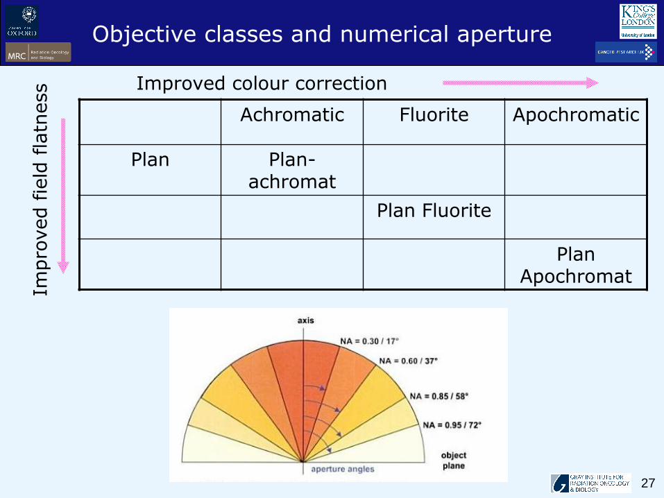
Objective classes and numerical aperture

Achromatic Fluorite Apochromatic

Plan Plan-achromat

Plan Fluorite

Plan Apochromat

Improved colour correction

Impro

ved fie

ld f

latn

ess

28

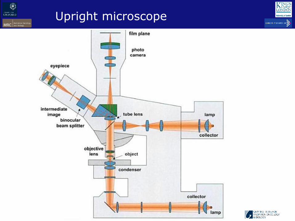
Upright microscope

29

Inverted microscope

30

Simplest of all the light microscopy techniques

Sample illumination is via transmitted white light, i.e. sample is illuminated from below and observed from above (or vice-versa)

Limitations include low contrast of most biological samples and low apparent resolution due to the blur of out of focus material

Simplicity of the technique and the minimal sample preparation required are significant advantages

Bright field microscopy

from: http://iheartguts.com/tag/brightfield-microscopy

31

Improves (and reverses) the contrast of unstained, transparent specimens

Uses a light source to minimize the amount of directly-transmitted (unscattered) light entering the imaging plane, collecting only the light scattered by the sample

Darkfield can dramatically improve image contrast—especially of transparent objects – while requiring little equipment setup or sample preparation

Suffers from low light intensity in final image of many biological samples, and provides low apparent resolution

Rheinberg illumination is a variant of dark field illumination transparent, coloured filters are inserted just before

the condenser light rays at high aperture are differently coloured

than those at low aperture (e.g. specimen background is red while the object appears yellow)

Dark field microscopy

annulusdisc condenser

objective

condenser

objective

sample

32

Gives the image a 3-dimensional appearance and can highlight otherwise invisible features

Technique based on this method is Hoffmann's modulation contrast, often used on inverted microscopes applied to cell culture work

Oblique illumination suffers poor contrast of many biological samples; low apparent resolution due to out of focus regions), but nevertheless can highlight otherwise invisible structures

Oblique illumination

light from condenser

sample

objective

objective

light ‘wedge’

http://www.microscopy-uk.org.uk

http://www.modulationoptics.com/

33

Widely used technique that shows differences in refractive index as difference in contrast

Developed by Frits Zernike in late 1930s (awarded the Nobel Prize in 1953)

Contrast is excellent but limited to imaging of thin objects

Halo is formed even around small objects, which obscures detail

Uses circular annulus in the condenser which produces a cone of light

This cone is superimposed on a similar sized ring within the phase-objective

Every objective has a different size ring: every objective requires appropriate condenser setting

Ring in the objective has special optical properties

Reduces the direct light in intensity

Creates an artificial phase difference of ~ /4

Since properties of this direct light have changed, interference with the diffracted light takes place: the result is a phase contrast image.

Phase contrast microscopy

phase

plate

objective

sample

condenser

annulus

complementary

rings

diffracted

rays

34

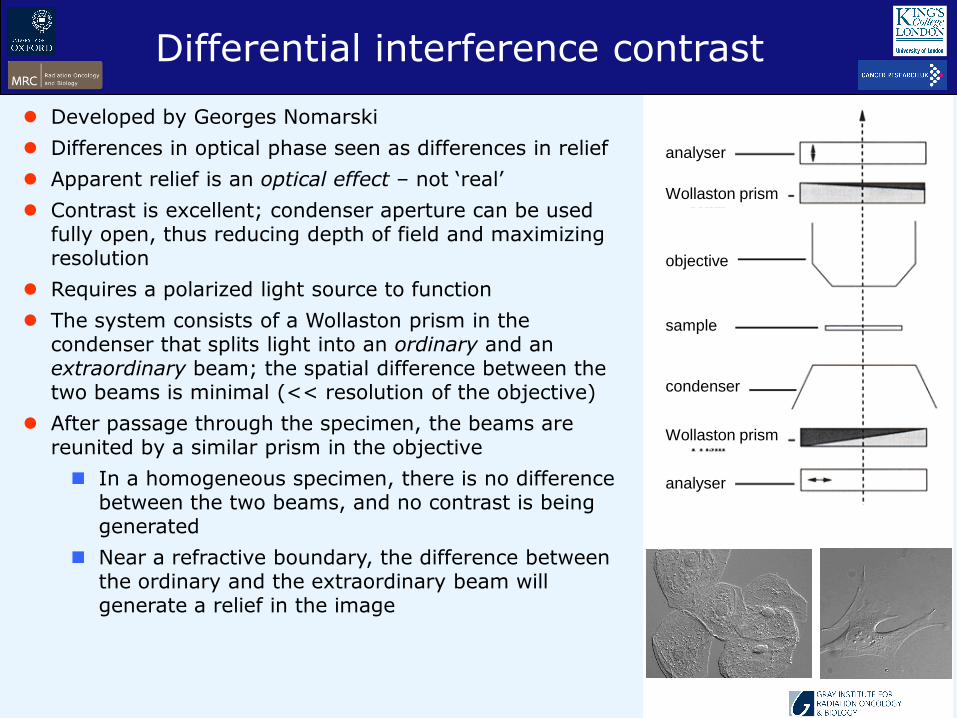
Developed by Georges Nomarski

Differences in optical phase seen as differences in relief

Apparent relief is an optical effect – not ‘real’

Contrast is excellent; condenser aperture can be used fully open, thus reducing depth of field and maximizing resolution

Requires a polarized light source to function

The system consists of a Wollaston prism in the condenser that splits light into an ordinary and an extraordinary beam; the spatial difference between the two beams is minimal (<< resolution of the objective)

After passage through the specimen, the beams are reunited by a similar prism in the objective

In a homogeneous specimen, there is no difference between the two beams, and no contrast is being generated

Near a refractive boundary, the difference between the ordinary and the extraordinary beam will generate a relief in the image

Differential interference contrast

analyser

Wollaston prism

objective

sample

condenser

Wollaston prism

analyser

35

DIC vs. phase contrast

analyser

Wollaston prism

objective

sample

condenser

Wollaston prism

analyser

image planeimage plane

Phase-

contrast

objective

objective

sample

condenser

undiffracted

light

diffracted

light

36

Modern microscopes provide ‘easy’ solutions for microphotography and electronic image recording.

Experienced microscopists often prefer a hand drawn image rather than a photograph

subject knowledge allows accurate conversion of an image into a precise drawing: a camera provides a single in-focus plane

The creation micrographs requires a monocular microscope

both eyes are open

the eye not observing down the microscope is concentrated on a sheet of paper besides the microscope

Without moving the head or eyes, record the observed details by tracing round the observed shapes by simultaneously ‘seeing’ the pencil point in the microscope image

Image recording

37

Time-lapse microscopy

Inverted microscope configuration

Incubator around the microscope

Control of temperature, humidity and pH (CO2)

Challenges: preserving focus, power outages (!)

38

When certain compounds are illuminated with high energy (blue) light, they emit light of a different, lower frequency (redder light)

This effect is referred to as fluorescence, or more generally luminescence

Almost all biological specimens have their own characteristic autofluorescence, based on their chemical makeup

Fluorescence microscopy is of critical importance in modern life sciences

Extremely sensitive, allows detection of single molecules

Many different fluorescent dyes can be used to stain different structures

A particularly powerful method is the combination of antibodies coupled to a fluorochrome as in immunostaining

Antibodies can be tailored specifically for a chemical compound

e.g. artificial production of proteins, based on the genetic code (DNA): used to immunize e.g. rabbits, form antibodies which bind to the protein. The antibodies are then coupled chemically to a fluorochrome and can be used to trace the proteins in the cells under study

Highly-efficient fluorescent proteins such as the green fluorescent protein(GFP) have been developed using gene fusion (process which links the expression of the fluorescent compound to that of the target protein)

Fluorescence microscopy

39

Fluorescence emission differs in wavelength from the excitation light: a fluorescence image ideally only shows labelled structure of interest

High specificity led to the widespread use of fluorescence light microscopy in biomedical research

Fluorescence dyes of different spectral characteristics used to stain different biological structures: simultaneous detection while still exhibiting specificity but differentiated from individual dye colour

Most fluorescence microscopes are operated in the epi-illumination mode (illumination and detection from one side of the sample) to decrease the amount of excitation light entering the imaging device

Fluorescence microscopy

40

Sequence of events leading to fluorescence

From: http://micro.magnet.fsu.edu

41

arc lamp

Johann Ploem

Dichromatic cube

Epi-illuminated fluorescence microscope

‘cube’

objective

42

Modern inverted fluorescence microscope

43

Objective

Specimen

Objective back

focal Plane

Eye

Eyepiece

Tube Lens

Intermediate

Image plane

or camera plane

Emission Filter

Dichromatic

Mirror

Excitation

Filter

Lamp

Arc

arc images

Condenser

Diaphragm

Field

Diaphragm

arc image

MICROSCOPE EPI-FLUORESCENCE

KÖHLER ILLUMINATION LIGHT PATHS

Collector Lens

Ftube‘4f’ telescope

lenses

determines area

of sample

illuminateddetermines

condenser

excitation

intensity

F1

F2F1

SCAN MIRROR HERE IN

BEAM SCANNING SYSTEM

Filter Cube

44

Under some circumstances, e.g. photobleaching or the presence of salts of heavy metals, etc., emitted light may be significantly reduced or stopped altogether

Fading - There are conditions that may affect the re-radiation of light and thus reduce the intensity of fluorescence. This reduction of emission intensity is generally called fading.

Fading is subdivided into quenching and bleaching

Bleaching is irreversible decomposition of the fluorescent molecules because of light intensity in the presence of molecular oxygen

Fluorescent probe molecule reports

‘classified’ information on behaviour of

surrounding molecules

Quenching also results in reduced fluorescence intensity and frequently comes about as a result of oxidizing agents or the presence of salts of heavy metals or halogen compounds

Sometimes quenching results from the transfer of energy to other so-called acceptor molecules physically close to the excited fluorophores, a phenomenon known as resonance energy transfer.

Fluorescence limitations

45

Fluorophore molecule can emit typ. 103 - 104 quanta

signal-to-noise

ratio

spatial

resolution

speedThe three Ss or the

‘eternal fluorescence triangle’

Fluorescence photon budgets

Any of the three can be enhanced at the expense of the

other two

Available quanta can be resolved in time or in wavelength,

but only up to maximum available

46

106 molecules @ 1 M cell ≈ 1 pl

1010 photons per cell maximum

At max. excitation ≈ 1013 photons per sec

Fluorescence lifetimes ≈ 10-9 - 10-8 sec typical

Collection, QE limitations ≈ 1-10% photons ‘used’

108 -109 detected quanta per cell practical

At max. excitation ≈ 1011 -1012 photons per sec

s/n ratio ≈ 104 -105 for steady-state signal

Distributed over time, space

Fluorescence photon budgets

47

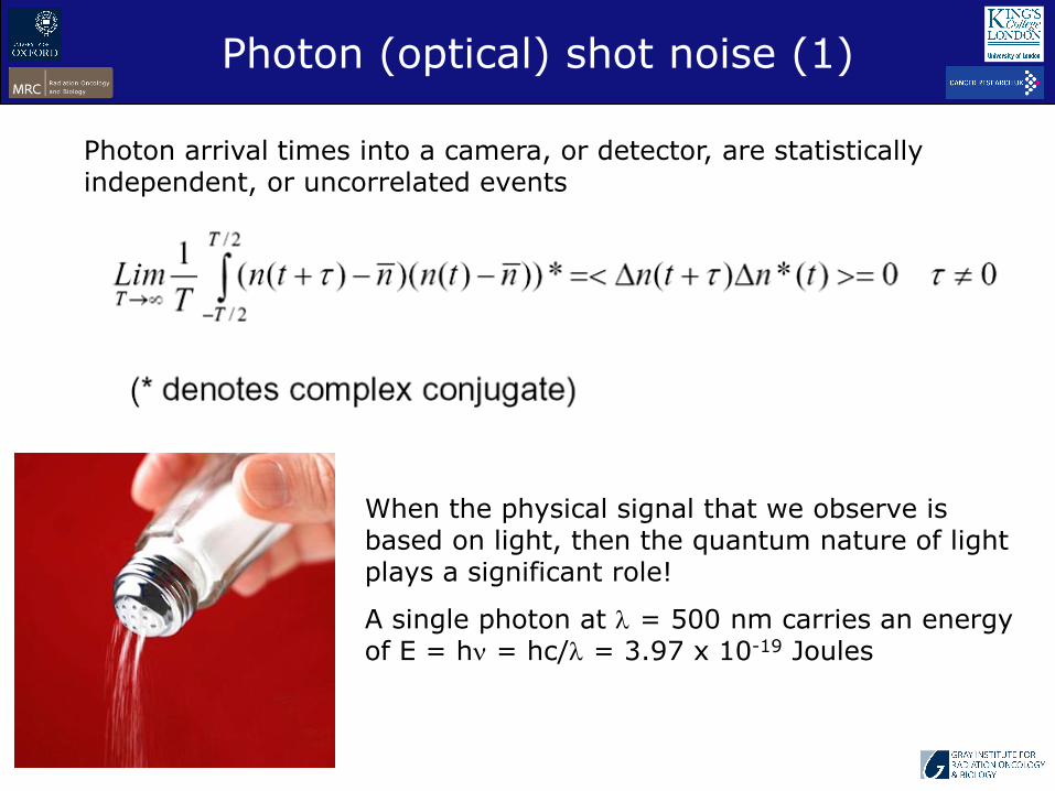
Photon (optical) shot noise (1)

Photon arrival times into a camera, or detector, are statistically independent, or uncorrelated events

When the physical signal that we observe is based on light, then the quantum nature of light plays a significant role!

A single photon at = 500 nm carries an energy of E = h = hc/ = 3.97 x 10-19 Joules

48

The intensity of a source will yield the average number of photons collected, but knowing the average number of photons which will be collected will not give the actual number collected

The actual number collected will be more than, equal to, or less than the average, and the distribution about that average will be a Poisson distribution

Cannot assume that, in a given pixel for two consecutive but independent observation intervals of length T, the same number of photons will be counted

The probability distribution for p photons in an observation window of length T seconds

where is the rate or intensity measured in photons per second

Photon (optical) shot noise (2)

49

Siméon Denis Poisson 1781-1840

1 photon4 photons10 photons

Poisson distribution

For sufficiently large numbers of photons, (typ. >>15-20) the normal (Gaussian) distribution with mean p and variance p (standard deviation p1/2), is a good approximation to the Poisson distribution.

FPoisson (x, p ) Fnormal (x; = p, 2 = p)

Johann Karl Friedrich Gauss 1777–1855

0 20 40 60 80 1000

0.02

0.04

0.06

0.08

0.1

0.1

0

P m n( )

1000 n

0 20 40 60 80 1000

0.02

0.04

0.06

0.08

0.1

0.1

0

G m n( )

1000 n

50

output

sensor

photons

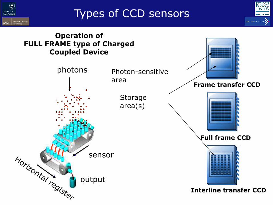
Operation of FULL FRAME type of Charged

Coupled Device

Frame transfer CCD

Full frame CCD

Interline transfer CCD

Types of CCD sensors

Photon-sensitive area

Storage area(s)

51

channels

channelsGlass

structure

input

photoelectronsecondary

electrons

glass

channel

wall

output

electrons

Semiconducting layer

Electrode

- High voltage +

Electrode plating (on each face)

Microchannel plate image intensifier

52

Electron multiplying CCD imager

EMCCD technology is a digital scientific detector innovation first introduced to the imaging community in early 2000, followed by spectroscopy versions in early 2005

As charge is transferred through each stage the phenomenon of impact ionization is utilized to produce secondary electrons, and hence EM gain

When this is done over several hundred stages, the resultant gain can be controlled from unity to hundreds or even thousands of times.

storage

section

imaging

section

o/p

charge-

voltage

conversion

Multiplication

register

readout

register

Unlike a conventional CCD, an EMCCD is not limited by the readout noise of the output amplifier.

a solid state Electron Multiplying (EM) register is added to the end of the normal serial register; it allows weak signals to be multiplied before any readout noise is added by the output amplifier

The EM register has several hundred stages that use higher than normal clock voltages

53

10.4 electrons pixel-1

0.8 electrons pixel-1

Electron multiplication – typ. x1000

EMCCD: the ‘ultimate’ camera?

54

Image generated in a completely different way to normal (wide-field) microscopy

Uses a scanning point (or points) of light instead of full sample illumination

Confocal microscopy provides significant improvements in optical sectioning by blocking the influence of out-of-focus light which would otherwise degrade the image

Confocal microscopy is commonly used where 3D structure is important or where out-of-focus light is to be rejected

Confocal microscopy

55

Rotating Nipkow disc

Fast image acquisition

Alternative and more commonly used arrangement uses scanning laser beams (LSM)

The rotating disc confocal microscope

Petran and Hadravsky: original dual-port optical system

56

Confocal imaging can offer a the resolution x1.4 wrt resolution obtained withconventional microscopes

A confocal microscope can be used in reflection mode and still exhibit the sameout-of-focus rejection performance – sometimes used for detecting goldparticles used in immuno-gold labeling

In a confocal imaging system a single point ofexcitation light (or sometimes a group of points or aslit) is scanned across the specimen. This is adiffraction-limited spot, produced either by imagingan illuminated aperture situated in a conjugate focalplane to the specimen or, more usually, by focusing aparallel laser beam

With only a single point illuminated, the illuminationrapidly falls off above and below the plane of focus asthe beam converges and diverges, thus reducingexcitation of fluorescence for interfering objectssituated out of the focal plane

Fluorescence light passes through a pinhole situatedin a focal plane conjugate to that of the specimen.Light passing through the image pinhole is detectedby a photodetector

Confocal microscopy

57

The laser-scanning confocal microscope

objective

dichromatic

mirror

photodetector

cell

pinhole 2

pinhole 1

laser beam

x

yscanning

spot moves in

x,y directions

light from only one

focal plane passes

through pinhole

58

Two-photon excitation - principle

two-photon excitation

single-photon excitation

300 400 500 600 700 800 900

59

Two-photon excitation – how it works

Only a single voxel is

excited at any one time

This excitation point is

scanned in x,y and z

and an image is built

up in a few seconds

An ultrashort laser

pulse is used for

excitation – very high

peak power, very low

average power

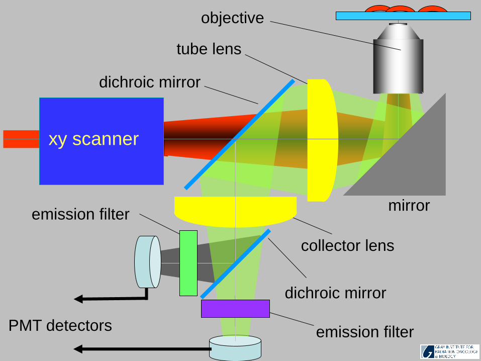
60

emission filter

xy scanner

objective

tube lens

mirror

dichroic mirror

emission filterPMT detectors

collector lens

dichroic mirror

61

emission filter

objective

tube lens

mirror

dichroic mirror

emission filterPMT detectors

collector lens

dichroic mirror

xy scanner

62

Ex vivo 2P imaging - rat gut

With 2P excitation, it is

possible to image

deeply into specimens,

(>>100 microns)

Image sequence of successive optically-sectioned layers

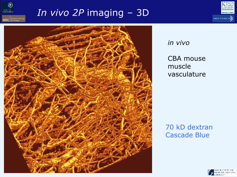
63

in vivo

CBA mouse muscle vasculature

70 kD dextranCascade Blue

In vivo 2P imaging – 3D

64

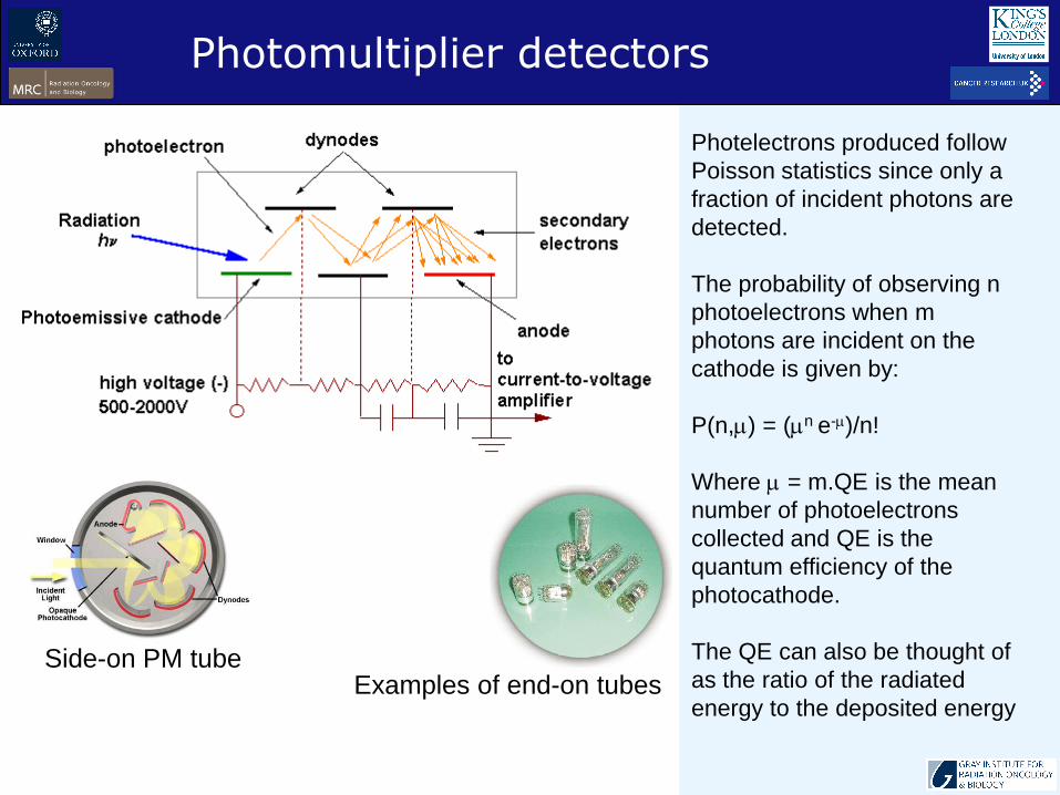
Photelectrons produced follow

Poisson statistics since only a

fraction of incident photons are

detected.

The probability of observing n

photoelectrons when m

photons are incident on the

cathode is given by:

P(n,) = (n e-)/n!

Where = m.QE is the mean

number of photoelectrons

collected and QE is the

quantum efficiency of the

photocathode.

The QE can also be thought of

as the ratio of the radiated

energy to the deposited energy

Photomultiplier detectors

Side-on PM tubeExamples of end-on tubes

65

The quantum efficiency (in %) at a given wavelength λ is related to the

radiant sensitivity R by:

QE = (124/λ) x R (measured in mA/W)

Photomultipliers

66

High quantum efficiency, high gainSmall active area

Avalanche photodiodes

Operation modes:

Linear: current to light intensityGeiger mode: pulse output

67

P22 fibrosarcoma

BD9 rat

Vasculature

(70 kD dextran / FITC)

+ autofluorescence

In vivo 2P imaging – 3D

68

Ex vivo 2P imaging

Mouse earMouse skin

69

P22 fibrosarcoma

BD9 ratHT29 human colon carcinoma

SCID mouse

70

High resolution, microvessel imaging

Liver

metastasis

formation

GFP tumour

cells

71

Fluorescence lifetime imaging

…..able to image molecular

interactions – and applied to

far-field methods with near-field

performance

72Intensity image Lifetime image

Kinetic trace at every pixel acquired (time resolution 130 ps)Kinetics analysed at every pixel to derive lifetime ()Lifetime mapped in (false colour) x (intensity)

Fluorescence lifetime imaging - FLIM

Analysis of the excited state lifetime of a

population of fluorescent probe molecules

Spatially resolved

acquisition of data

Informs on

molecular

environment

+

73

Donor emission

quenched

Protein

Donor

GFP

Protein

Acceptor-

labelled protein

Donor

GFP

Donor

emission

Főrster Resonance Energy Transfer (FRET)

FRET

Sensitized

emission

When donor emission spectrum overlaps with acceptor absorption spectrum

When dipole donor and acceptor moments are aligned Probability of FRET [separation]-6 (0.1-10 nm range)

74

Donor emission

quenched

Protein

Donor

GFPFRET

Sensitized

emission

Population of FRET species

= A1 / (A2+A1)

A1 = amplitude of quenched donor lifetime

A2 = amplitude of control donor lifetime

FRET efficiency

= (D - ) / D

D = control donor lifetime

= quenched donor lifetime

Unquenched

donor lifetime

D

Fully quenched

donor lifetime

Partial FRET

population

+ D

Főrster Resonance Energy Transfer (FRET)

75

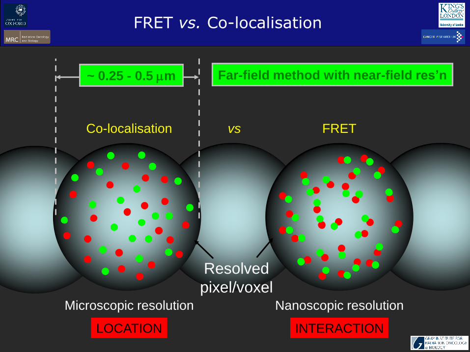
FRET vs. Co-localisation

~ 0.25 - 0.5 m

vs FRETCo-localisation

Microscopic resolution Nanoscopic resolution

LOCATION INTERACTION

Far-field method with near-field res’n

Resolved

pixel/voxel

76

TACdiscriminator

excitation

arrival time

photodetectors

discriminator ADC

reset

time address

memory

event

xy address

add

Time-correlated single photon counting

signal

reference

77

1

10

100

0 10 ns5.02.5 7.5

distribution

Intensity

imageLifetime

image

In vivo 2P lifetime imaging

78

Location of site of PAK1-Cdc42 interaction.

MP FLIM used to determine the extent of

FRET between the GFP-PAK1 donor and

anti-HA-Cy3 acceptor in cells co-expressing

GFP-PAK1 and HA-tagged Cdc42 (WT and

N17 variants).

FLIM/FRET example: GFP donor, Cy3 acceptor