OPTICAL ENCODING BASED ON

SINGLE PIXEL IMAGING

LEONG YONG EN

A project report submitted in partial fulfilment of the

requirements for the award of Bachelor of Engineering

(Honours) Electrical and Electronic Engineering

Lee Kong Chian Faculty of Engineering and Science

Universiti Tunku Abdul Rahman

April 2021

i

DECLARATION

I hereby declare that this project report is based on my original work except for

citations and quotations which have been duly acknowledged. I also declare that it

has not been previously and concurrently submitted for any other degree or award at

UTAR or other institutions.

Signature :

Name : LEONG YONG EN

ID No. : 1604408

Date : 8/5/2021

ii

APPROVAL FOR SUBMISSION

I certify that this project report entitled “OPTICAL ENCODING BASED ON

SINGLE PIXEL IMAGING” was prepared by LEONG YONG EN has met the

required standard for submission in partial fulfilment of the requirements for the

award of Bachelor of Engineering (Honours) Electrical and Electronic Engineering at

Universiti Tunku Abdul Rahman.

Approved by,

Signature :

Supervisor :

Date :

Signature :

Co-Supervisor :

Date :

Chua Sing Yee

9 May 2021

iii

The copyright of this report belongs to the author under the terms of the

copyright Act 1987 as qualified by Intellectual Property Policy of Universiti Tunku

Abdul Rahman. Due acknowledgement shall always be made of the use of any

material contained in, or derived from, this report.

© 2021, Leong Yong En. All right reserved.

iv

ACKNOWLEDGEMENTS

I would like to thank everyone who had contributed to the successful completion of

this project. I would like to express my gratitude to my research supervisor, Dr. Chua

Sing Yee for her invaluable advice, guidance and his enormous patience throughout

the development of the research.

v

ABSTRACT

Single Pixel Imaging (SPI) is an imaging framework that utilises only one light

detector instead of detector arrays required by conventional imaging sensors. This is

achieved by sequentially applying a series of mask patterns and measures the light

intensity using the single light detector. The measurements correspond to the mask

patterns can then be used to reconstruct the image. SPI is inherently encrypted, since

the light intensity collected cannot be related to the original image in any way or

form, and can only be reconstructed based on the mask patterns used. Thus, the

collected light intensities can be perceived as the ciphertext and the configuration of

mask patterns is the key.

Due to the inherent property of SPI, its encryption security and performance

were studied. The image acquisition and reconstruction are essentially optical

encoding and decoding process. Various SPI encoding and decoding schemes were

investigated, which include Hadamard, random, Fourier, and Chaotic. The findings

from the analysis of these existing schemes suggest the need of a new encryption

method. The proposed method is essentially a double encryption that utilises the

mixing of logistic chaotic maps using random index map at the first phase and

Double Random Phase Encoding (DRPE) or Rivest–Shamir–Adleman Encryption

(RSA) at the second phase. Assessment was performed from the perspectives of

reconstruction quality and security analysis. Besides, the proposed method was also

compared to the existing encryption schemes. The results show that the proposed

method has average performance in term of image reconstruction quality at low

sampling rate but has significant improvement in term of security. Therefore, the

proposed method is able to overcome the shortcomings regarding the security of

conventional SPI encoding schemes.

vi

TABLE OF CONTENTS

DECLARATION i

APPROVAL FOR SUBMISSION ii

ACKNOWLEDGEMENTS iv

ABSTRACT v

TABLE OF CONTENTS vi

LIST OF TABLES ix

LIST OF FIGURES x

LIST OF SYMBOLS / ABBREVIATIONS xii

LIST OF APPENDICES xiv

CHAPTER

1 INTRODUCTION 1

1.1 General Introduction 1

1.2 Importance of the Study 1

1.3 Problem Statement 2

1.4 Aims and Objectives 2

1.5 Scope and Limitation of the Study 3

1.6 Contribution of the Study 3

1.7 Outline of the Report 3

2 LITERATURE REVIEW 4

2.1 Introduction 4

2.2 Single Pixel Imaging 5

2.3 Compressed Sensing (CS) 6

2.4 Optical Image Encryption 7

2.4.1 Double Random Phase Encoding 7

2.5 Rivest–Shamir–Adleman Encryption (RSA) 9

vii

2.6 Chaotic Maps 10

2.7 Similar Studies 12

2.7.1 A Novel Compressive Optical Encryption via

Single-Pixel Imaging 12

2.7.2 Compressive optical steganography via single-pixel

imaging 15

2.8 Attacks on Encrypted Single Pixel Imaging 18

2.9 Summary 20

3 METHODOLOGY AND WORK PLAN 21

3.1 Introduction 21

3.2 Simulation Tool 21

3.3 Investigation of SPI Encoding Methods 21

3.3.1 Process Flow 22

3.3.2 Evaluation Metrics 23

3.4 Proposed New Encryption Method 26

3.4.1 First Phase 27

3.4.2 Second Phase 29

3.5 Project Planning 31

3.6 Summary 31

4 RESULTS AND DISCUSSIONS 33

4.1 Introduction 33

4.2 Comparisons Between Present Methods 33

4.2.1 Reconstruction Quality 37

4.2.2 Security 42

4.3 Comparisons Between Proposed Method 48

4.3.1 Reconstruction Quality 48

4.3.2 Security 49

4.4 Overall Comparisons 53

4.5 Summary 58

5 CONCLUSIONS AND RECOMMENDATIONS 60

viii

5.1 Conclusions 60

5.2 Recommendations for future work 60

REFERENCES 62

APPENDICES 65

ix

LIST OF TABLES

Table 4.1: Reconstruction results for image A 34

Table 4.2: Reconstruction results for image 0 35

Table 4.3: Reconstruction results for image 7 36

Table 4.4: Reconstruction results for image cameraman 37

Table 4.5: Tabulated reconstruction quality metrics for different

SPI encoding schemes 38

Table 4.6: Security measurement metric values of all encoding

methods 43

Table 4.7: Quality metrics for SPI-DRPE and SPI-RSA 49

Table 4.8: Results of security analysis 50

Table 4.9: Reconstructed images for image A 53

Table 4.10: Reconstructed images for image 0 54

Table 4.11: Reconstructed images for image 7 55

Table 4.12: Reconstructed images for image cameraman 55

x

LIST OF FIGURES

Figure 2.1: Illustration of SPI system 4

Figure 2.2: Signal acquisition process based on CS (Rani, Dhok

and Deshmukh, 2018) 7

Figure 2.3: Optical implementation of DRP (Alfalou and

Brosseau, 2009) 8

Figure 2.4: Logistic model result, by growth rate. (Boeing, 2016) 11

Figure 2.5: Bifurcation diagram of logistic map. (Boeing, 2016) 12

Figure 2.6: (a)RIM. (b)Cosine fringe corresponding to a value of

1 in the RIM. (c)Optical encryption system based

on SPI. (Zhang, et al., 2019a) 13

Figure 2.7: Relationship between M and CC for simulation and

experiment (Zhang, et al., 2019a) 14

Figure 2.8: Overall look of the steganography system (Zhang, et

al., 2019) 15

Figure 2.9: Flowchart of the steganography(Zhang, et al., 2019) 17

Figure 3.1: Images used for simulation. 22

Figure 3.2: Flowchart of the simulation 22

Figure 3.3: Histogram of secure cryptosystem: (a)plaintext,

(b)ciphertext 25

Figure 3.4: Overall flow of encryption and decryption of the

proposed system 26

Figure 3.5: Mixing process of the logistic map 27

Figure 3.6: Flowchart of the mixing algorithm 28

Figure 3.7: (a)Encryption process of DRPE, (b)Decryption

process of DRPE 29

Figure 3.8: Gantt chart 31

Figure 4.1: Average RMSE of all reconstructed images at

different sampling ratio 40

xi

Figure 4.2: Average PSNR of all reconstructed images at

different sampling ratio 40

Figure 4.3: Average SSIM of all reconstructed images at different

sampling ratio 41

Figure 4.4: Average CC of all reconstructed images at different

sampling ratio 42

Figure 4.5: Histogram of ciphertext and plaintext when using

Hadamard method for image: (a) A, (b) 0, (c) 7, (d)

cameraman 44

Figure 4.6: Histogram of ciphertext and plaintext when using

random method for image: (a) A, (b) 0, (c) 7, (d)

cameraman 45

Figure 4.7: Histogram of ciphertext and plaintext when using

Fourier method for image: (a) A, (b) 0, (c) 7, (d)

cameraman 46

Figure 4.8: Histogram of ciphertext and plaintext when using

chaotic logistic method for image: (a) A, (b) 0, (c)

7, (d) cameraman 47

Figure 4.9: Histogram of final ciphertext and plaintext when

using SPI-DRPE method for image: (a) A, (b) 0, (c)

7, (d) cameraman 51

Figure 4.10: Histogram of final ciphertext and plaintext when

using SPI-RSA method for image: (a) A, (b) 0, (c)

7, (d) cameraman 52

Figure 4.11: Average RMSE for different sampling ratio 56

Figure 4.12: Average PSNR for different sampling ratio 57

Figure 4.13: Average SSIM for different sampling ratio 57

Figure 4.14: Average CC for different sampling ratio 58

xii

LIST OF SYMBOLS / ABBREVIATIONS

(x, y) pixel position

∅ SPI measurement matrix

⨂ convolution

a luminance weightage

A, B 2-dimentional distribution

b contrast weightage

c column index

c structure weightage

CQ ciphertext

eps minimum value to prevent zero error

Km illumination pattern

M number of measurements

MAXI maximum value of pixel of image

N number of pixels

OQ plaintext

r row index

x image vector

zfi processed pixel value

zoi initial pixel value

Ω solid angle of the light cone

𝑖 complex number

𝑣, 𝜇, 𝜉, 𝜂 frequency

𝛼 sparse coefficient

𝜎 noise

𝜑 sparse basis

𝜑(𝑛) Euler’s totient function

ART Arnold transform

CC correlation coefficient

COA ciphertext-only attack

CPA chosen plaintext attack

xiii

CS compressed sensing

DRPE double random phase encoding

FPA focal point array

FRT fractional Fourier transform

FST Fresnel transform

FT Fourier Transform

GPRA generalized phase retrieval algorithm

GT Gyrator transform

HT Hartley transform

IM index map

JT jigsaw transform

KPA known phase attack

LCT linear canocical transform

MP modulated patterns

MSE mean square error

OMP orthogonal matching pursuit

PSNR peak signal to noise ratio

RIM random index map

RMSE root mean square error

RSA Rivest-Shamir-Adleman

SNR signal to noise ratio

SPI single pixel imaging

SSIM structural similarity index

TC total curvature

TV total variation

xiv

LIST OF APPENDICES

APPENDIX A: Simulation codes 65

1

CHAPTER 1

1 INTRODUCTION

1.1 General Introduction

Single Pixel Imaging (SPI) is an optical imaging method where image acquisition is

done by only a single pixel detector. In comparison with modern digital cameras,

silicon focal point array (FPA) sensor is used to detect an image which is made up of

millions of pixels (Edgar, Gibson and Padgett, 2019). One might ask how can a

single pixel detects and reconstruct an image when the pixel can only detect the

intensity of light. This is done by illuminating the target image with arrays of

patterned light, and then recording the array of intensity of light with a single pixel

detector. The light pattern and the light intensity array recorded can be used to

reconstruct the image based on algorithms and principles of compressed sensing (CS).

Based on the image reconstruction method stated just now, it is observed that

SPI imaging is basically going through an encoding and decoding process. For every

image acquisition and reconstruction, the key is the pattern array. Thus, SPI is

inherently more secure compared to conventional imaging methods. Encoding or

encryption is the recording of information with the intention of hiding its true

information and only authorise the true information to the intended or authorised

person with the decoding key. Encryption of information can be dated back to

ancient times where secret information are being transmitted as symbols and sketches.

Thus, this project will study the optical encoding based on SPI to further improve the

security of the SPI scheme.

1.2 Importance of the Study

SPI method is a fast-growing field that is studied by many researchers. The reason

for this is that industrial application requires low costing cameras, SPI provides this

advantage as only one-pixel sensor is needed to record the image. This advantage is

further amplified when recording non-visible light spectrum images as light detector

that is outside of the visible spectrum is significantly more expensive than the normal

detectors. It is also notable that SPI is able to sense compressively, therefore

reducing the data storage and data transferring requirements (Edgar, Gibson and

Padgett, 2019).

2

In this study, the main focus is on the encoding of SPI. The inherent

advantage of SPI can be further enhanced. By improving the security of the SPI

scheme, SPI scheme might become the leading optical imaging method for secret

image transfer. Thus, studies are to be done on the performance of encryption

methods in order to evaluate its feasibility so that it can be referenced to in the future

when developing a more secured, cost effective and high-performance SPI encoding

scheme.

1.3 Problem Statement

Encryption of information needs to be updated and new encryption methods need to

be introduced as new attacking methods are developed. Thus, to make sure that the

secret image is secured, new SPI encoding method can be studied. Besides security,

the performance of the encoding scheme must also be considered. Most encoding

method will cause some alteration to the image when the image is encoded and

decoded. Thus, performance analysis is needed to identify the quality of the image

retrieved. Although there are multiple studies regarding SPI encoding methods, there

is lack of comprehensive security analysis as they are mainly focus on quality

analysis. For instance, “A Novel Compressive Optical Encryption via Single-Pixel

Imaging” by Zhang et al. (2019a). Therefore, multiple security analysis is done to fill

in this research gap.

1.4 Aims and Objectives

In order to solve the problem statement mentioned above, three objectives for this

project have been identified.

1. To review the SPI and different encoding and decoding schemes. This is

important to establish a comprehensive understanding on SPI as well as

different encoding methods.

2. Design a novel encryption method based on SPI to improve the security of

encryption.

3. To analyse the performance of the designed method and available methods.

This validated and proves the feasibility of the method.

3

1.5 Scope and Limitation of the Study

The scope of this study includes the literature review of SPI, image performance

analysis, encryption security and multiple encryption methods. In particular,

encoding and decoding process of SPI were investigated. It is hoped to propose a

secure double encryption method as part of the study. Accordingly, the proposed

method was compared with other SPI encryption methods to compare its

performance using suitable metrics.

In this study, MATLAB was used as the main tool to simulate the results.

Selected datasets that are adequate for the study were used and analysed. No physical

test bench will be constructed. Thus, there will be limitation to the result as some

real-world conditions might not be considered in the simulations.

1.6 Contribution of the Study

The project will contribute to the research gap of the security evaluation of SPI

encoding framework. Many data in information on the SPI encoding, its strengths

and weaknesses will be explored and revealed. Besides that, a more secure SPI based

encryption framework is developed in order to overcome the shortcoming of

available SPI encoding methods. Through this project, further understanding is

gained in terms of the security and the potential of SPI in image cryptography.

1.7 Outline of the Report

This report is divided into five chapters. The first chapter introduces the problem

statement and objectives of the project. Chapter 2 reviews SPI and other encoding

frameworks. It also reviews the Mathematic theory that is often used in encryption.

Besides, similar studies that are relevant to this project is also studied. Next, Chapter

3 presents the work flow of the simulation, the software used for the simulation,

security and quality evaluation metrics used, and the methodology of the proposed

encryption method. Chapter 4 displays the result and discussion of the project. It is

separated into available SPI encoding method simulations and proposed encryption

method simulation results and comparisons. Finally, Chapter 5 concludes the whole

project and gives insight to what can be improved and the limitation of the project.

4

CHAPTER 2

2 LITERATURE REVIEW

2.1 Introduction

The most popular image acquisition method in the market right now is based on

sensor arrays, and pixel counts in cameras nowadays have become a performance

metric as well as marketing strategy. Though, the developing SPI method is found to

have some competitive advantages compared to the conventional cameras.

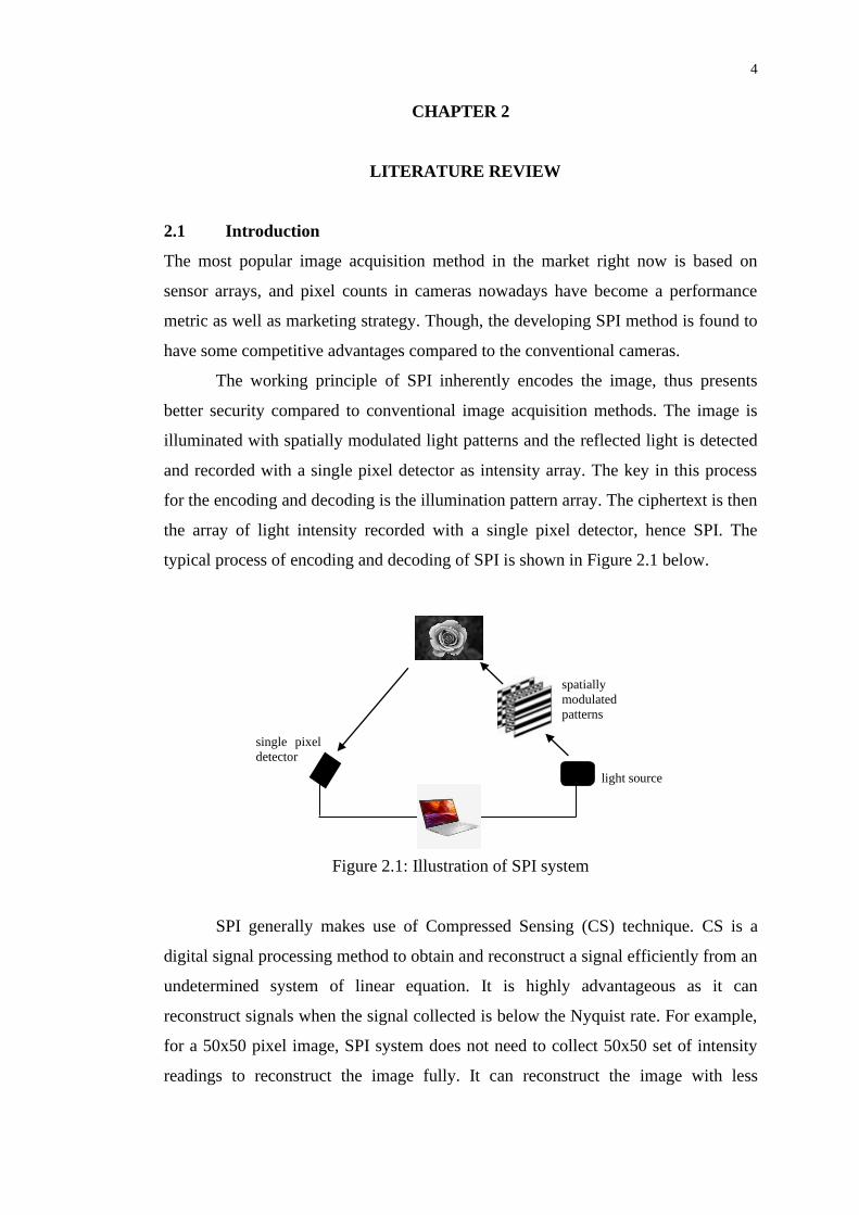
The working principle of SPI inherently encodes the image, thus presents

better security compared to conventional image acquisition methods. The image is

illuminated with spatially modulated light patterns and the reflected light is detected

and recorded with a single pixel detector as intensity array. The key in this process

for the encoding and decoding is the illumination pattern array. The ciphertext is then

the array of light intensity recorded with a single pixel detector, hence SPI. The

typical process of encoding and decoding of SPI is shown in Figure 2.1 below.

SPI generally makes use of Compressed Sensing (CS) technique. CS is a

digital signal processing method to obtain and reconstruct a signal efficiently from an

undetermined system of linear equation. It is highly advantageous as it can

reconstruct signals when the signal collected is below the Nyquist rate. For example,

for a 50x50 pixel image, SPI system does not need to collect 50x50 set of intensity

readings to reconstruct the image fully. It can reconstruct the image with less

light source

spatially

modulated

patterns

single pixel

detector

Figure 2.1: Illustration of SPI system

5

readings. The condition to use CS is that the signal is inherently sparse in some

domain. In a natural image, this criterion is fulfilled as its wavelet domain is sparse

(Rani, Dhok and Deshmukh, 2018).

In the literature review, details of SPI and CS will be discussed. Besides,

studies that have similar objectives as this project is reviewed.

2.2 Single Pixel Imaging

SPI is an image acquisition and reconstruction method that utilizes CS concepts to

reconstruct the image. As mentioned before, the image acquisition method is using

masked patterns to form illumination patterns onto the target image and the light

intensity is recorded. To cater the compressed sensing reconstruction, the masks

pattern used are considered.

It is generally common to use a method that does not match the spatial

properties of the image, such as random pattern (Edgar, Gibson and Padgett, 2019).

Though, this method usually takes more time and can make the reconstruction time

to greatly exceed the acquisition time. Thus, this method is not suitable for

applications that requires real time performance.

The other approach on the mask pattern is to use pattern that are not totally

incoherent with the spatial properties of the image, such as the Hadamard or Fourier

masks. This method trades some image quality for speed, thus are more suitable for

real time applications (Edgar, Gibson and Padgett, 2019).

Mathematically, image, denoted as x can be considered as a 𝑁 × 1 matrix of

N unknown intensities. The mask pattern basis is denoted as ∅, which is a 𝑀 × 𝑁

matrix of 0 and 1 to represent the transmitted and blocked light. The measured signal

is y, which is the product of x and ∅, which is expressed in the Eq. (2.1).

𝑦 = ∅𝑥 (2.1)

The image x is sparse in nature, thus are represented by a sparse basis 𝜑 and

its coefficient which are the uncompressed image denoted by 𝛼 which is K-sparse.

This means that only K number of coefficients in 𝛼 are non-zero. The equation of x

is shown in Eq. (2.2).

𝑥 = 𝜑𝛼 (2.2)

6

Thus, the equation of the measured signal becomes

y=∅φα (2.3)

The measurement basis matrix ∅ should be maximally incoherent with the

sparse basis 𝜑, such as using random binary pattern (Edgar, Gibson and Padgett,

2019). In order to reconstruct the image when the number of measurements is less

than pixels M < N some CS algorithms are used. The image in the transform domain

can be reconstructed when the number of sampling patterns used is 𝑀 ≥

𝑂(𝐾𝑙𝑜𝑔 (𝑁

𝐾)) by solving an optimization problem (Edgar, Gibson and Padgett, 2019).

One of the optimization methods that can be used are the ℓ1 minimization, which can

be expressed as

𝛼∗ = arg 𝑚𝑖𝑛||𝛼||1 𝑠𝑢𝑏𝑗𝑒𝑐𝑡 𝑡𝑜 𝑦 = ∅𝜑𝛼 (2.4)

where the pixel domain representation of image 𝑥∗ can be calculated through

𝑥∗ = 𝜑𝛼∗ (2.5)

There are also other optimization methods that can be used such as the total variation

(TV) minimization and the total curvature (TC) minimization.

For real life practice, the data measured will be suspected to noise 𝜎 which

comes from the instability of light source and electronic readout noise from the

detector. Thus, the equation considering the noise are represented by

𝛼∗ = arg 𝑚𝑖𝑛||𝛼||1 𝑠𝑢𝑏𝑗𝑒𝑐𝑡 𝑡𝑜 ||𝑦 − ∅𝜑𝛼||2 ≤ 𝜎 (2.6)

2.3 Compressed Sensing (CS)

CS is developed and introduced by Donoho, Candes, Romberg and Tao in 2004 and

is used for the acquisition of sparse or compressible signals (Rani, Dhok and

Deshmukh, 2018). Sparsity means that the signal has only few significant parts,

where most of the data is equal or close to zero. This method saves data storage as

most traditional signal acquisition methods need to follow the Nyquist criterion,

causes too many redundant data is recorded when the signal is sparse. CS enable

signal acquisition and deconstruction that discards the non-significant data, thus

taking fewer measurements.

7

The image acquisition algorithm in 2.2 is essentially the compressed sensing

signal acquisition algorithm. Number of measurement matrix M is less than the

length of input signal N. Due the sparse property of natural image, the complete

reconstruction can be done using CS with M proportional with sparsity of image K.

Figure 2.2 shows the acquisition process based on CS.

Figure 2.2: Signal acquisition process based on CS (Rani, Dhok and Deshmukh,

2018)

2.4 Optical Image Encryption

Optical encoding takes advantage of the coherent nature of the laser beam to obtain

efficient encrypted data as well as high speed decryption through parallel processing

(Glückstad and Palima, 2009). It is also able to encrypt information in multiple

dimensions.

2.4.1 Double Random Phase Encoding

One very important optical encryption technique that serves as the basis for many

optical encryption methods now is the double random phase encoding (DRPE)

(Alfalou and Brosseau, 2009).

The general idea of this technique is encrypting the image into a stationary

white noise by altering its spectrum. In DRPE, both amplitude and phase spectrum

are altered to encrypt the information securely, since there are ways to reconstruct

the image with only phase or amplitude information (Alfalou and Brosseau, 2009).

The process can be mathematically explained as follows. the image represented by

I(x, y) are to be multiplied with a first key which is a random phase mask RP1. RP1

can be expressed as

𝑅𝑃1 = exp(𝑖2𝜋𝑛(𝑥, 𝑦)) (2.7)

where

8

n(x, y) = white noise that are uniformly distributed in [0, 1]

After that, it is multiplied by a second encryption key which is a second random

phase mask in Fourier domain. The key is expressed as

𝑅𝑃2 = exp(𝑖2𝜋𝑏(𝑣, 𝜇)) (2.8)

where

𝑏(𝑣, 𝜇) = white noise that is uniformly distributed in [0, 1] independent of 𝑛(𝑥, 𝑦)

In this way, the image is encrypted. The encryption process that fully represents the

process is

𝐼𝑐(𝑥, 𝑦) = (𝐼(𝑥, 𝑦) exp(𝑖2𝜋𝑛(𝑥, 𝑦)))⨂ℎ(𝑥, 𝑦) (2.9)

where

⨂ = convolution

ℎ(𝑥, 𝑦) = 𝐹𝑇−1[𝑅𝑃2]

This method can be implemented optically through a setup illustrated in Figure 2.3

below, where the lenses perform Fourier transform (FT) optically.

Figure 2.3: Optical implementation of DRP (Alfalou and Brosseau, 2009)

To decode the encrypted image, FT of Ic(x, y) is multiplied with conjugate of

RP2. Then, its inverse FT will be |𝐼(𝑥, 𝑦) exp(𝑖2𝜋𝑛(𝑥, 𝑦)) |2 = |𝐼(𝑥, 𝑦)|2.

Besides using FT for DRP, different types of transforms such as fractional

Fourier transform (FRT), Fresnel transform (FST), linear Canonical transform (LCT),

Gyrator transform (GT), and Hartley transform (HT) can also be used (Liu, Guo and

Sheridan, 2014).

9

2.5 Rivest–Shamir–Adleman Encryption (RSA)

Rivest-Shamir-Adleman Encryption (RSA) is a public key cryptosystem which is

named after its developers. A public key cryptosystem, also known as asymmetric

cryptosystem, is done by using two different keys. The two keys are the public key

and the private key. The private key cannot be derived from the public key, which

makes it safe to publish the encryption key without risking the leak of the private key.

RSA cryptosystem utilises the property of field of number theory, where it is simple

to multiply two large prime numbers to generate a composite number, but it is very

hard to do the reverse (Zhao, et al., 2010). There is still no effective algorithm to do

an efficient decomposition yet.

In order to perform RSA, there are a few steps that need to be followed. First,

two distinct prime numbers, p and q are chosen and their product, n is calculated as

shown in Eq. (2.10)

𝑛 = 𝑝𝑞 (2.10)

Next, encryption key, e is generated where it should be less than the Euler’s totient

function 𝜑(𝑛) and more than 1. e must also be the coprime of 𝜑(𝑛). The Euler

totient function 𝜑(𝑛) is expressed as

𝜑(𝑛) = (𝑝 − 1)(𝑞 − 1) (2.11)

Finally, the decryption key, d is calculated. The calculation is shown in Eq. (2.12)

𝑑 = 𝑒−1𝑚𝑜𝑑 𝜑(𝑛) (2.12)

The public key is (e, n) while the private key is (d, n). The private key, d must be

kept secret. The values of p, q, and 𝜑(𝑛) should also be kept secret because it is

possible to calculate the private key using these values.

After preparing the keys, the encryption and decryption process can be

performed. The encryption and decryption process can be represented by Eq. (2.13)

and Eq. (2.14) respectively.

𝑐 = 𝑚𝑒(𝑚𝑜𝑑 𝑛) (2.13)

𝑚 = 𝑐𝑑(𝑚𝑜𝑑 𝑛) (2.14)

where

10

c = ciphertext

m = plaintext

The security of RSA relies on the difficulty to factorize integers. In this case,

the difficulty to factorise n. Factorising n to p and q is the most obvious way to attack

the cryptosystem. But as mentioned before, this is a very hard problem to be solved.

This is especially true when n is large. Thus, p and q should be large enough so that

it is more secure, subjecting to the specific usage of the encryption (Zhou and Tang,

2011).

2.6 Chaotic Maps

Chaotic map is a mapping that exhibits chaotic characteristics. It is derived from

chaos theory which is a branch of mathematics that handles nonlinear dynamical

systems (Boeing, 2016). The term nonlinear indicates that the change in the system

output is not proportional to the input due to feedback or multiplicative effects.

Meanwhile, dynamical systems indicates that the system changes over time

depending on the current state. Chaotic systems exhibit random like behaviour. It

may be derived from a simple looking equation with few interactive parts but it is

very sensitive to initial conditions and can result in a completely different sequence

when a very small change is applied to it. Despite their deterministic simplicity, as

the system changes over time the output can become extremely unpredictable and

divergent.

The unpredictable, random, and sensitivity to key nature of the chaotic

systems makes it a highly studied and applied technique for encryption (Agarwal,

2018). There are many kinds of different chaotic maps that are utilised for encryption.

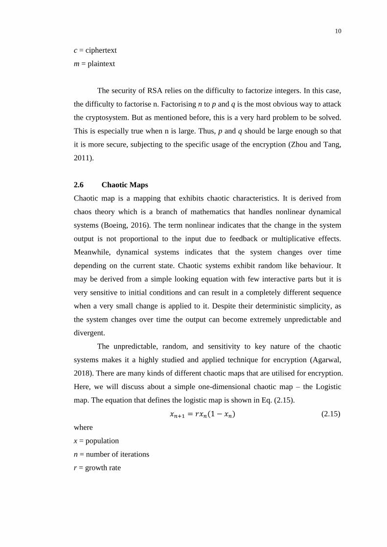
Here, we will discuss about a simple one-dimensional chaotic map – the Logistic

map. The equation that defines the logistic map is shown in Eq. (2.15).

𝑥𝑛+1 = 𝑟𝑥𝑛(1 − 𝑥𝑛) (2.15)

where

x = population

n = number of iterations

r = growth rate

11

Growth rate is a very important parameter as the population might not be

chaotic at certain growth rate. For instance, with growth rate of 0.5, the population

will settle to 0 after many iterations. The relationship between the population and

generations of iteration based on different growth rate are shown in Figure 2.4. Note

that the population starts with 0.5 in this example.

Figure 2.4: Logistic model result, by growth rate. (Boeing, 2016)

Attractor is the value where the system settles toward after many iterations. In

the case where growth rate is 0.5, the system will have one point attractor at 0. When

the growth rate is less than 3.5, the logistic system is not yet chaotic since it only has

limited number of attractor that the system oscillates around. When growth rate is

more than 3.5, the system will have a strange attractor where the system will oscillate

forever and will not repeat or settle to a steady state. A bifurcation diagram shows

this more clearly as it plots the relationship between the attractor and the growth rate.

The bifurcation diagram of logistic map is shown in Figure 2.5.

12

Figure 2.5: Bifurcation diagram of logistic map. (Boeing, 2016)

2.7 Similar Studies

2.7.1 A Novel Compressive Optical Encryption via Single-Pixel Imaging

Zhang et al. (2019a) proposed a novel compressive optical encryption via SPI. The

study involves the theory of their encryption and results, both in simulation and real-

life experiment with an optical setup.

The key of their proposed SPI encryption lies in the random index map (RIM)

which consists of 0 and 1s. The RIM is generated as the secret key. The column and

row index of the 1s in the RIM corresponds to a Fourier basis subset which forms the

measurement matrix ∅ mentioned in the SPI explanation. Thus, we can say that the

RIM has the information of illumination pattern encrypted. The illustration of the

system is shown in Figure 2.6.

13

Figure 2.6: (a)RIM. (b)Cosine fringe corresponding to a value of 1 in the RIM.

(c)Optical encryption system based on SPI. (Zhang, et al., 2019a)

To explain the relationship between the pattern and RIM, assume that a

256x256 RIM is generated with 16000 1s. The row index is denoted as r and column

index as c. When there is a 1 in the RIM, its row and column index will be used to

formulate the cosine and sine fringes in the Fourier basis. It is expressed as

𝑝𝑐(𝜇, 𝑣) = cos[2𝜋𝑐𝜇 + 2𝜋𝑟𝑣] (2.16)

𝑝𝑠(𝜇, 𝑣) = sin[2𝜋𝑐𝜇 + 2𝜋𝑟𝑣] (2.17)

where

𝑝𝑐(𝜇, 𝑣) = cosine fringe

𝑝𝑠(𝜇, 𝑣) = sine fringe

The fringes are then generated by computer and the light with fringes pattern are

projected to the target image. Its resulting signal can be expressed as

𝐼(𝜇, 𝑣) = 𝑝(𝜇, 𝑣)𝑥(𝜇, 𝑣) (2.18)

where

𝑝(𝜇, 𝑣) = ps or pc

𝐼(𝜇, 𝑣) = reflectance function of the target image

14

By recording all of the signals with a single pixel detector, the result can be

expressed as

𝑦(𝑖) ∫ 𝑝𝑖(𝜇, 𝑣)𝑥(𝜇, 𝑣)𝑑𝜇𝑑𝑣Ω

(2.19)

This is analogous to the SPI scheme expressed in equation (2.1), where x is the

column vector reshaped from 𝑥(𝜇, 𝑣), ∅ represents the measurement matrix whose

rows is the fringe 𝑝(𝜇, 𝑣) that are reshaped to a row. In this case, ∅ will be a 32000 x

65536 matrix while y will be a 32000 x 1 column matrix.

The decryption method used in this study utilizes TV minimization. The

decryption process can be expressed as Eq. (2.3).

The result obtained from simulation and experiment are compared using a

metric called correlation coefficient (CC). The result of CC ranges from 0 to 1 where

0 is the worst and 1 is the best. Zhang et al. (2019a) experimented with the number of

sampling done, denoted by M. The results of simulation and experiment are shown in

Figure 2.7.

Figure 2.7: Relationship between M and CC for simulation and experiment (Zhang,

et al., 2019a)

Besides quality analysis, the writer also analysed their cryptosystem by

attempting to crack the ciphertext in 3 ways, namely the inverse FT of ciphertext,

using counterfeit RIM and brute force search of the correct RIM. For the first two

methods, the ciphertext cannot be decrypted and gives out a noise pattern result. For

15

brute search of known RIM, the number of permutations is too large that the

ciphertext cannot be decoded in short time.

To conclude the study, Zhang et al. (2019a) has successfully designed a SPI

encryption method that is secure and has high reconstruction quality.

2.7.2 Compressive optical steganography via single-pixel imaging

Zhang, He et al. (2019) has suggested compressive optical steganography via SPI.

Steganography is a method whereby the secret information is hidden inside another

source of data that is not suspicious. In this study, Zhang et al. (2019b) designed a

steganography technique via SPI, and made simulations and experiments to analyse

the performance of the technique.

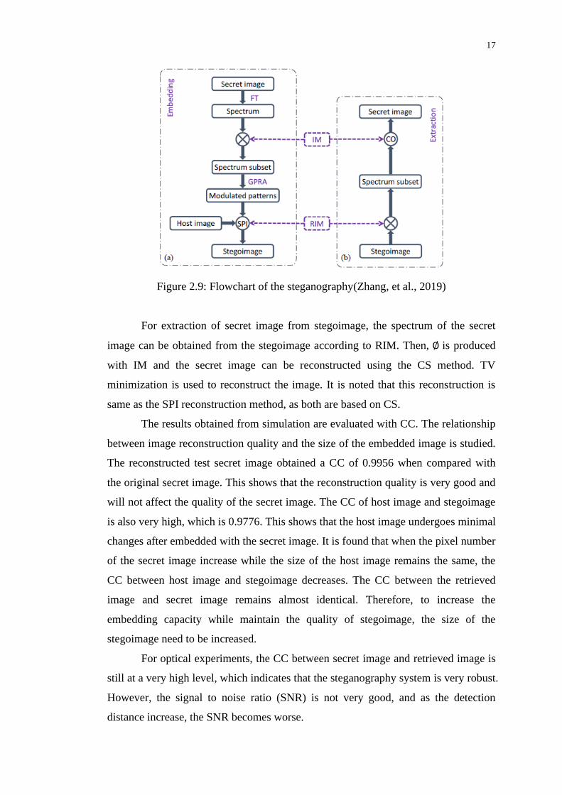
The steganography proposed by Zhang et al. (2019b) can be explained in two

parts, the embedding and extraction of information. In the embedding process, an

image secret image is concealed inside a host image. The host image can be decoded

by anyone with inverse FT. The secret image can only be accessed using the correct

key. The overall look on the system is shown in Figure 2.8.

Figure 2.8: Overall look of the steganography system (Zhang, et al., 2019)

The secret image is first undergone FT. To embed the secret image, an index

map (IM) of 180x180 pixels is generated. In the IM there are 5265 1s. Indices of the

IM is used to form a 10530x32400 measurement matrix denoted by ∅. The secret

image is sparse sampled with ∅ just like the SPI method shown in equation 2.1. The

resulting data is compressed, where the compressed data is denoted as y.

After that, y is embedded into the Fourier spectrum of the host image which

has a resolution of 256x256 pixels. The embedding process is done according to a

16

RIM which represents the secret key. Modulated patterns (MP) need to be

constructed to embed the host image using the SPI system. The MP which contains

the information to the secret image is used to illuminate the host image to enable the

image to be acquired by a SPI system. The result of the acquired signal can be

expressed as Eq. (2.20).

𝑦(𝑖) = ∫ ℎ(𝜇, 𝑣)𝑀𝑃(𝜇, 𝑣)𝑑𝜇𝑑𝑣Ω

(2.20)

where

𝑀𝑃(𝜇, 𝑣) = modulated patterns

ℎ(𝜇, 𝑣) =host image.

Based on the integral property of FT, Eq. (2.19) can be expressed as

𝑦(𝑖) = 𝐹𝑇[ℎ(𝜇, 𝑣)𝑀𝑃(𝜇, 𝑣)](𝜉, 𝜂)|𝜉=0,𝜂=0 (2.21)

The MP can be found by using a generalized phase retrieval algorithm (GPRA). The

algorithm is repeated until the MP converges. The algorithm is done in 3 steps.

Firstly, a MPk is generated for initialization. Then FT is performed on

ℎ(𝜇, 𝑣)𝑀𝑃𝑘(𝜇, 𝑣) and the constrain shown in Eq. (2.21) is imposed. Lastly, inverse

FT is done on the result in step 2 to get hmupdate. It will be used to calculate the new

MP. The update calculation can be expressed as

𝑀𝑃𝑘+1 =ℎ𝑚𝑢𝑝𝑑𝑎𝑡𝑒

ℎ(𝑢,𝑣)+𝑒𝑝𝑠 (2.22)

where

eps = minimum to prevent zero error

The flowchart of the steganography is shown in Figure 2.9.

17

Figure 2.9: Flowchart of the steganography(Zhang, et al., 2019)

For extraction of secret image from stegoimage, the spectrum of the secret

image can be obtained from the stegoimage according to RIM. Then, ∅ is produced

with IM and the secret image can be reconstructed using the CS method. TV

minimization is used to reconstruct the image. It is noted that this reconstruction is

same as the SPI reconstruction method, as both are based on CS.

The results obtained from simulation are evaluated with CC. The relationship

between image reconstruction quality and the size of the embedded image is studied.

The reconstructed test secret image obtained a CC of 0.9956 when compared with

the original secret image. This shows that the reconstruction quality is very good and

will not affect the quality of the secret image. The CC of host image and stegoimage

is also very high, which is 0.9776. This shows that the host image undergoes minimal

changes after embedded with the secret image. It is found that when the pixel number

of the secret image increase while the size of the host image remains the same, the

CC between host image and stegoimage decreases. The CC between the retrieved

image and secret image remains almost identical. Therefore, to increase the

embedding capacity while maintain the quality of stegoimage, the size of the

stegoimage need to be increased.

For optical experiments, the CC between secret image and retrieved image is

still at a very high level, which indicates that the steganography system is very robust.

However, the signal to noise ratio (SNR) is not very good, and as the detection

distance increase, the SNR becomes worse.

18

2.8 Attacks on Encrypted Single Pixel Imaging

In order to understand more about the security of SPI encoding, the attack method on

SPI is studied. In this section, a study done by Jiao et al. (2019) titled “Known-

Plaintext Attack and Ciphertext-Only Attack for Encrypted Single-Pixel Imaging” is

reviewed.

The usual attacks on image encryption are the chosen-plaintext attack (CPA),

known-plaintext attack (KPA) and ciphertext-only attack (COA). In terms of CPA,

assumption is made that the attacker is able to access to the encryption system and

dictate the input plaintext. Key can be recovered by selecting a few pair of ciphertext

and plaintext and analyse it. This attack is not analysed because the situation where

the attacker can access to the encryption system is not likely. For KPA, the attacker

has a few random plaintext-ciphertext pairs. This situation happens more in real life

situations and can poses higher threat. For COA, the attacker only has a few

ciphertext and does not have any information on plaintext. COA analysis on an

encryption system is very important because it can reveal serious problem on the

cryptography system as it indicates that the system only needs very few information

to be cracked. This method is the hardest to implement for an attacker.

Now, KPA on encrypted SPI system will be analysed. Plaintext can only be

retrieved from the ciphertext with the correct key. It is high risk when the same key

is repeatedly used to encrypt an image. The attacker can find out the key from

analysing the cyphertext intensity sequences and collect its plaintext pair. The way of

finding the key which is the illumination pattern similar to the way of reconstruction

of SPI image. Assume the “illumination patterns” are plaintext images and the

“plaintext image” as an illumination pattern. This can be illustrated in Eq. (2.23)

(2.23)

where

OQ = plaintext, Q = 1, 2, …, M

Km = illumination pattern

CQ = ciphertext.

19

This is analogous to Eq. (2.1). Thus, the mth illumination pattern can be found using

SPI reconstruction method. Once all illumination pattern from m = 1 to m = M is

found, the illumination patterns are put combined together to form ∅ which is the

MxN SPI measurement matrix, the key to the encryption system.

For COA on encrypted SPI system, only the ciphertext are known. Recovery

using that little information is extremely hard. In the experiment done by Jiao et al.

(2014), they only found an algorithm to crack the SPI encoding key when under

certain conditions. The conditions are that the pixel values of illumination patterns

before permutation are known, and assumption is made that the same category of

images are repetitively encrypted with SPI. The attacker can collect many example

images that are similar to the actual encrypted image. To find the original

illumination pattern permutation sequence, the attacker can use the example images

and use the known illumination pattern to illuminate the image and record its

intensity. After finishing this process with all known illumination pattern, the

intensities data recorded is compared with its ciphertext counterpart. The

illumination pattern will be arranged based on the best fitting match. Thus, the key is

retrieved.

The key cracked using KPA is very accurate as based on the experiment done

by Jiao et at. (2014), the key recovered shows very high similarity that exceeds 99.8%

compared to the original key. When using the cracked key to decode the test image,

the reconstructed image has acceptable quality with a peak signal to noise ratio

(PSNR) of over 16dB. This KPA scheme can only be successfully done when the

plaintext-ciphertext pairs are enough, which is equal to M. When encrypted image is

decrypted using a random key, noise like image is retrieved. Thus, it can be said that

the SPI system has good security when the key is not known.

For the key cracked with COA, the scheme proposed by Jiao et al. (2014)

produces key in which its effectiveness decreases as the image size increases. When

the ciphertext and example image pair increase, the quality of the key retrieved from

the scheme will increase. In the proposed COA scheme, the plaintext must be similar

and belong to the same category in order to successfully find out the key. if the

plaintext is totally of different category, none of the illumination pattern will be

recovered in the correct order (Jiao, et al., 2019) .

20

2.9 Summary

In this literature review, many important information related to SPI encoding and

optical encryption are studied. The mathematics part of SPI, CS, DRPE, RSA, and

chaotic systems are studied in order to fully understand and implement the

information in this study. Besides that, a few studies related to the project are

discussed. Literatures are reviewed to get a fundamental background and improve

planning in this project. The security of SPI is also analysed by analysing the attack

method and effectiveness to fully understand the security of SPI. The research gap

noticed when studying the literature is the lack of in-depth encryption system studies

on SPI. This is the reason that this project will try to tackle the under researched area

by developing a new SPI based encryption system and analyse its performance.

21

CHAPTER 3

3 METHODOLOGY AND WORK PLAN

3.1 Introduction

In this chapter, the simulation framework for our investigation is explained. Besides,

the steps done to compare different SPI encoding methods are explained. The quality

and security measurement method are also presented. Furthermore, the proposed new

SPI based encryption method is explained clearly in order to enable future

reproduction of results. Lastly, the planning of this project, is shown through the

Gantt chart.

3.2 Simulation Tool

The development of double encryption method and the experiment to evaluate its

performance are done fully through simulation. MATLAB is used because of its

powerful numerical computation functions especially on matrices, which involved

heavily in image processing. The SPI encoding schemes that are commonly used,

namely Hadamard, Fourier and random sampling can be simulated by functions

available in MATLAB. For instance, N Hadamard masks can be produced by using

hadamard(N) function easily.

For CS reconstruction schemes, some common approaches such as L1

optimization, TV optimization and matching pursuit can also be performed easily

with MATLAB. The libraries for the optimization methods are available in

MATLAB, thus simplifying the process. For instance, l1dantzig_pd function is used

as a L1 minimization method to reconstruct the final image.

3.3 Investigation of SPI Encoding Methods

Four existing SPI encoding methods namely Hadamard, random, Fourier and chaotic

logistic are chosen and simulated using MATLAB, which are explained in the next

section. Four different images are used as test image for SPI encoding. The images

that are used for simulation is shown in Figure 3.1. Each image is simulated four

times with sampling ratio of 0.25, 0.5, 0.75, and 1. This is to evaluate the

performance of the encryption at different sampling ratio, as one of the advantages of

22

SPI is it utilises CS so that image can be reconstructed with less information than

conventional imaging framework.

Figure 3.1: Images used for simulation.

3.3.1 Process Flow

The methods investigated in this project are Hadamard, random, Fourier, and chaotic.

The process flow of the simulation of these methods are shown in Figure 3.2.

First, an image is encoded with SPI method using the patterns stated. Subsequently,

security analysis is performed on the ciphertext to evaluate its security. The metrics

used for the security measurement are further explained in Section 3.3.2. After that,

the image is reconstructed through L1 optimisation. L1 optimisation is chosen

because it has the best security as compared to TV minimization and OMP (Xiong, et

Sampling ratio:

0.25, 0.5, 0.75, 1

Sampling ratio:

0.25, 0.5, 0.75, 1

Sampling ratio:

0.25, 0.5, 0.75, 1

Sampling ratio:

0.25, 0.5, 0.75, 1

Encrypt

Encrypt

Encrypt

Encrypt Decrypt

Decrypt

Decrypt

Decrypt

Figure 3.2: Flowchart of the simulation

23

al., 2020). Finally, performance analysis is done on the reconstructed image by using

the original image as the reference. That is further explained in Section 3.3.2.

3.3.2 Evaluation Metrics

Data obtained from experiments must be evaluated quantitatively in order to give

unbiased results and justify the performance comparison.

Our key concerns are efficiency, quality, robustness towards noise and

security. Efficiency can be quantified through the image reconstruction time. Quality

of image produced can be evaluated by using root mean square error (RMSE),

structural similarity index (SSIM), peak signal to noise ratio (PSNR), and correlation

coefficient (CC).

In RMSE, mean square error (MSE) is square rooted. MSE is the average

difference of pixel between the original image and a processed image. Therefore,

RMSE measures the accuracy of the processed image compared to the original image.

The equation of RMSE is shown below

𝑅𝑀𝑆𝐸 = ∑ [(𝑧𝑓𝑖−𝑧𝑜𝑖)

2

𝑁]

0.5𝑁𝑖=1 (3.1)

where

𝑧𝑓𝑖 = processed value

𝑧𝑜𝑖 = original value

SSIM is a perceptual metric that measures the deterioration of image from the

original image. Similar to RMSE, values of original image and processed image are

needed to calculated SSIM. SSIM evaluates the visible structure of the image, and

thus are closer to human perception of similarity. The equation of SSIM in shown

below

𝑆𝑆𝐼𝑀 = [𝑙(𝑥, 𝑦)𝑎. 𝑐(𝑥, 𝑦)𝑏. 𝑠(𝑥, 𝑦)𝑐] (3.2)

where

𝑙(𝑥, 𝑦) = luminance

𝑐(𝑥, 𝑦) = contrast

𝑠(𝑥, 𝑦) = structure

𝑎, 𝑏, 𝑐 = weightage of l, c and s respectively

24

PSNR represents the ratio of maximum possible power of a signal and the

power of noise in the signal. This means that the higher the PSNR, the better

reconstructed image is. PSNR is represented in decibels. The equation representing

PSNR is shown below.

𝑃𝑆𝑁𝑅 = 20 log(𝑀𝐴𝑋𝐼) − 10log (𝑀𝑆𝐸) (3.3)

where

𝑀𝐴𝑋𝐼 = maximum value of pixel of the image

CC is a measure of the relationship between two signals. It tries to calculate

the probability of linear relationship between two signals. This is metric is not only

used in signal processing but also statistics. The equation of CC is shown below

𝐶𝐶 =∑ ∑ (𝐴𝑟𝑐−)(𝐵𝑟𝑐−𝑐𝑟 )

√(∑ ∑ (𝐴𝑟𝑐−)2𝑐 )(∑ ∑ (𝐵𝑟𝑐−)2

𝑐 )𝑟𝑟 (3.4)

where

A, B = two different 2D distributions

r, c = indexes of the rows and columns respectively

Next, security measurement metrics are discussed. The methods selected to

measure the security of the encryption are histogram analysis, key space analysis,

and differential attack analysis. These methods can be visualised and quantified, thus

are selected for the security analysis.

Histogram analysis shows the histogram of pixel intensity values. It counts

the number of pixels at different intensities that are found in the image. For an 8-bit

grayscale image, there are 256 different intensity values. The intensity histogram

displays the distribution of pixel intensity in the image based on the 256 intensity

values. In a secure encryption, the intensity of the ciphertext should be evenly

distributed and different from the histogram of the original image in order to not leak

any information to potential attackers (Jiao, et al., 2020). The example the histogram

of a secure cryptosystem is shown in Figure 3.3.

25

Figure 3.3: Histogram of secure cryptosystem: (a)plaintext, (b)ciphertext

Histogram analysis is also quantifiable. This is possible by calculating the variance

distribution of the histogram. Small variance means that the histogram is distributed

evenly, hence more secure.

Next measurement of security used is the key space analysis. Key space

analysis is performed by calculating all the possible set of keys for the encryption.

The higher the key space value, the stronger the cryptosystem is against brute force

attacks. Key space calculation does not have a specific formula and depends on the

cryptosystem itself. For instance, an encryption uses 2 keys and the values of the

keys are discrete values that ranges from 1 to 100. Then, the key space of that

encryption will be 100 × 100 = 10000. A cryptosystem needs at least a key space

of 1030 in order to be considered as robust (Heucheun Yepdia, Tiedeu and Kom,

2021).

The last security measurement method used in this project is the differential

attack analysis. Differential attack analysis is done by changing the plaintext slightly

and compare its ciphertext with respect to the original plaintext’s ciphertext. In a

good cryptosystem, the slightest change of plaintext should cause a large change in

the ciphertext. There are two metrics that can measure the effect of a slight change of

the plaintext over the ciphertext, which are the number of pixel change rate (NPCR)

and the unified average change intensity (UACI). The equation of these is shown in

Eq. (3.5) and Eq. (3.6) respectively.

𝑁𝑃𝐶𝑅 =∑ 𝐷(𝑖,𝑗)𝑖,𝑗

𝑀×𝑁× 100%, (3.5)

𝑤ℎ𝑒𝑟𝑒 𝐷(𝑖, 𝑗) = 1 𝑤ℎ𝑒𝑛 𝐶(𝑖, 𝑗) ≠ 𝐶′(𝑖, 𝑗), 𝑒𝑙𝑠𝑒 𝐷(𝑖, 𝑗) = 0

𝑈𝐴𝐶𝐼 =1

𝑀×𝑁[∑

|𝐶(𝑖,𝑗)−𝐶′(𝑖,𝑗)|

255𝑖,𝑗 ] × 100 (3.6)

(a)

(a)

(a)

(a)

(b)

(b)

(b)

(b)

26

where

C = ciphertext before slight change

C’ = ciphertext after slight change

(i, j) = pixel index of the image

M, N = length and width of the image, in pixel count

NPCR measures the rate of change of pixel values in the ciphertext when one pixel

of the plaintext is changed. UACI measures the average change of the intensity value

of ciphertext when one pixel of plaintext is changed. The expected value of NPCR

and UACI are 99.6094070 and 33.463507 respectively (Liu and Ding, 2020). This

means that good cryptosystem is expected to have NPCR and UACI that are close to

those values.

3.4 Proposed New Encryption Method

The proposed new encryption method consists of two encryption process. The first

phase encryption is an SPI encoding that utilises a mixed logistic chaotic map as its

mask pattern. Second phase of encryption uses either DRPE or RSA encryption.

Both of them are tested and compared. The overall flow of the encryption and

decryption process is shown in Figure 3.4.

Figure 3.4: Overall flow of encryption and decryption of the proposed system

27

3.4.1 First Phase

The first phase is the SPI encoding phase. The mask patterns used as the key is

derived from a bipolar logistic map. Since the logistic map produces values that

ranges from 0 to 1, the system is made bipolar by following the condition 𝑥 = 1

when 𝑥 ≥ 0.5 and 𝑥 = 0 when 𝑥 < 0.5. Two bipolar logistic maps with two different

initial condition of size 𝑀 × 𝑁 is created where M is the number of sampling

measurements and N is the number of pixels of the image. Next, another bipolar

logistic map of length M is created and is used as a random index map (RIM) to mix

the first two logistic map. The first logistic map A is first chosen as the current map.

The first row of the current logistic map is used as the first mask pattern array. The

subsequent mask pattern is determined by RIM. If the value of RIM = 1, it continues

to take the next row from the current map. If the value of RIM = 0, the current map

switches to the another logistic map and the rows are taken from it. This process

continues for M iterations. After M rows are taken, the measurement matrix is

completed. Each row of the measurement matrix is the mask pattern. The illustration

of the mixing of logistic maps to form the measurement matrix and the flowchart of

the mixing algorithm are shown in Figure 3.5 and 3.6 respectively.

Logistic

map A

Logistic

map A

Logistic

map A

Logistic

map A

Logistic

map B

Logistic

map B

Logistic

map B

Logistic

map B

Mixed logistic

matrix

(measurement

matrix)

Mixed logistic

matrix

(measurement

matrix)

Mixed logistic

matrix

(measurement

matrix)

Mix the rows

according to RIM

Mix the rows

according to RIM

Mix the rows

according to RIM

Mix the rows

according to RIM

Chaotic

mask

pattern

Chaotic

mask

pattern

Chaotic

mask

pattern

Chaotic

mask

pattern

Take each row

Take each row

Take each row

Take each row

Figure 3.5: Mixing process of the logistic map

28

Figure 3.6: Flowchart of the mixing algorithm

29

3.4.2 Second Phase

The second phase of the encryption either uses DRPE or RSA.

DRPE is reviewed in Section 2.4.1. Let us assume that the result from the

first phase encryption is the plaintext here. In this application, the process is done by

multiplying the plaintext with a random phase mask RP1 that is expressed in Eq.

(2.7). The size of n(x,y) in Eq. (2.7) must match the size of the plaintext. After that,

the result undergoes a fast Fourier transform (FFT). Next, it is multiplied by a second

random phase mask RP2 that is expressed as in Eq. (2.8). Similarly, the size of

𝑏(𝑣, 𝜇) must be the same as the size of the plaintext. Finally, it undergoes inverse

FFT to get the final ciphertext. For the decryption, the final ciphertext undergoes

FFT and then it is multiplied with the conjugate of RP2. Next, it undergoes inverse

FFT and then the magnitude of the result will be the plaintext. The encryption and

decryption process of DRPE is depicted in Figure 3.7.

Figure 3.7: (a)Encryption process of DRPE, (b)Decryption process of DRPE

30

For RSA encryption, the cryptosystem is initially designed for encrypting

strings in ASCII code. Some modifications are needed in order to perform RSA on

an image. Note that all the multiplication done here is element wise multiplication.

First, the two initial prime numbers p and q are randomly chosen for each

pixel of the plaintext (result from first phase encryption). The prime numbers are

limited to the 3rd prime to the 30th prime only and their product, n must be larger than

255. This is because the calculation of the encryption and decryption of RSA

involves getting the remainder when divided by n. Since image intensity values range

from 0 to 255, n must be at least 256 to obtain the correct reconstructed value will be

correct. After the selection of suitable prime numbers, all the needed parameters are

calculated for each pixel based on Eq. (2.10), (2.11), and (2.12). The encryption

considers complete. The public key, private key and n for RSA image encryption are

expressed as in Eq. (3.7).

𝑒 = [

𝑒1,1 𝑒1,2 …𝑒2,1 𝑒2,2 …… … 𝑒𝑖,𝑗

], 𝑑 = [

𝑑1,1 𝑑1,2 …

𝑑2,1 𝑑2,2 …

… … 𝑑𝑖,𝑗

], 𝑛 = [

𝑛1,1 𝑛1,2 …𝑛2,1 𝑛2,2 …… … 𝑛𝑖,𝑗

] (3.7)

where

e = public key

d = private key

n = modulus

i, j = plaintext size in pixel

The encryption and decryption are done by following Eq. (2.13) and (2.14)

for each of the pixel of the plaintext. Before encryption, the result from the first

phase encryption needs to be converted from 0-1 to 0-255. This is done by

multiplying it by 255 and obtaining the integer part. Its decimal part is recorded into

an array. The array is added after the decryption process to prevent information loss.

The final ciphertext are expressed as grayscale intensities. Since the encryption

process may produce ciphertext that are more than 255, some modifications need to

be done in order to keep the ciphertext below 256 without information loss. This is

done by utilising Eq. (3.8)

𝑐 = 256𝑘 + 𝑟 (3.8)

where

c = original ciphertext

31

k = multiple constant

r = remainder

The remainder will be used as the final result of the encryption. Eq. (3.8) is used to

retrieve the original ciphertext without losing any information. Due to this, c and k

need to be passed along with the decryption key d in order to decrypt r.

3.5 Project Planning

The project planning is done by creating a Gantt chart shown in Figure 3.8 to ensure

that improtant milestones are achieved in time so that good results can be produced

in time. The Gantt chart shows the time allocated for each important milestone

throughout the 14 week time span.

Figure 3.8: Gantt chart

3.6 Summary

The process flow of SPI encoding methods such as Hadamard, random, Fourier, and

logistic chaotic is presented. The newly proposed encryption method is also

explained in detail. The new encryption method is a double encryption which utilises

SPI at the first phase and DRPE or RSA at the second phase. For the first phase, the

mixing of logistic maps with RIM as the measurement matrix of the SPI is the

modification to improve the encoding security. In the second phase, DRPE or RSA is

used. For RSA which is initially designed for encrypting strings in ASCII code, it is

modified to suit image encryption. Overall performance will be evaluated using CC,

32

RMSE, PSNR, and SSIM in term of image quality. Meanwhile histogram analysis,

key space analysis, and differential attack analysis will be performed to evaluate its

security capability. The Gantt chart is also made to plan work ahead of time.

33

CHAPTER 4

4 RESULTS AND DISCUSSIONS

4.1 Introduction

In this chapter, the results of the simulation of different SPI encoding methods will

be presented and discussed. The SPI encoding methods will be evaluated based on its

reconstruction quality and security. The advantage of each method will be examined.

After that, the results of the proposed method will be presented and reviewed. Since

there are two different encryption method in the second phase, the performance

based on quality and security will be compared and discussed. Issues presented by

the method will also be assessed. Finally, the proposed method will be compared

with the of the conventional SPI encoding methods in order to visualise and discuss

the advantages and potential drawbacks of the proposed methods.

4.2 Comparisons Between Present Methods

Methods that are compared are Hadamard, random, Fourier and chaotic logistic. The

results of the reconstruction for image A, 0, 7, and cameraman are shown in Table

4.1, 4.2, 4.3, and 4.4 respectively. Via visual observation of the reconstructed images,

we can see that the image reconstruction quality becomes better as the sampling ratio

increases. This is because there is more information that are available to reconstruct

the image. All images are still recognisable at all sampling ratio. It is notable that the

Hadamard method has the worst reconstruction quality at sampling ratio of 1. It is

also noticeable that the Fourier method has the best reconstruction quality at lower

sampling ratio. All of these observations are only based on visual inspection and will

be further verified by using the proper quality measurement methods.

34

Table 4.1: Reconstruction results for image A

Sampling ratio

(M/N)

0.25 0.5 0.75 1

Original image

Reconstructed

image

(Hadamard)

Reconstructed

image

(Random)

Reconstructed

image

(Fourier)

Reconstructed

image (Chaotic

logistic)

35

Table 4.2: Reconstruction results for image 0

Sampling ratio

(M/N)

0.25 0.5 0.75 1

Original image

Reconstructed

image

(Hadamard)

Reconstructed

image

(Random)

Reconstructed

image

(Fourier)

Reconstructed

image (Chaotic

logistic)

36

Table 4.3: Reconstruction results for image 7

Sampling ratio

(M/N)

0.25 0.5 0.75 1

Original image

Reconstructed

image

(Hadamard)

Reconstructed

image

(Random)

Reconstructed

image

(Fourier)

Reconstructed

image (Chaotic

logistic)

37

Table 4.4: Reconstruction results for image cameraman

4.2.1 Reconstruction Quality

In this section, the reconstruction quality of the studied methods is discussed by

using RMSE, PSNR, SSIM, and CC. The data is tabulated in Table 4.5 for all

measuring metrics for different sampling ratio.

Sampling ratio

(M/N)

0.25 0.5 0.75 1

Original image

Reconstructed

image

(Hadamard)

Reconstructed

image

(Random)

Reconstructed

image

(Fourier)

Reconstructed

image (Chaotic

logistic)

38

Table 4.5: Tabulated reconstruction quality metrics for different SPI encoding

schemes

Method Image M/N RMSE PSNR SSIM CC

Hadamard

A

1 0.10781 19.347 0.3739 0.84816

0.75 0.13834 17.181 0.31773 0.801

0.5 0.22272 13.045 0.25882 0.66705

0.25 0.30048 10.444 0.18743 0.50954

0

1 0.35003 9.1178 0.18247 0.74565

0.75 0.35575 8.9771 0.15967 0.68542

0.5 0.43398 7.2507 0.13348 0.58513

0.25 0.43745 0.71814 0.082424 0.45747

7

1 0.34052 9.3573 0.15393 0.75023

0.75 0.31519 10.029 0.12889 0.69167

0.5 0.37772 8.4566 0.10867 0.6274

0.25 0.47769 6.4171 0.090723 0.47802

cameraman

1 0.21778 13.239 0.43648 0.85303

0.75 0.21004 13.554 0.39565 0.78479

0.5 0.21974 13.162 0.35618 0.6789

0.25 0.19836 14.051 0.3 0.5858

Method Image M/N RMSE PSNR SSIM CC

random

A

1 0.060912 24.306 0.89809 0.99987

0.75 0.10662 19.443 0.33747 0.84129

0.5 0.17773 15.005 0.22867 0.6948

0.25 0.26677 11.477 0.15214 0.50325

0

1 0.075699 22.418 0.31885 0.99995

0.75 0.33858 9.4068 0.15742 0.82113

0.5 0.39093 8.158 0.11679 0.6515

0.25 0.44904 6.9543 0.078919 0.46348

7

1 0.079563 21.986 0.26204 0.99995

0.75 0.29743 10.532 0.153 0.80839

0.5 0.37138 8.6037 0.115 0.64459

0.25 0.43028 7.325 0.078264 0.44939

cameraman

1 0.028755 30.826 0.99075 0.99985

0.75 0.15753 16.053 0.36772 0.85763

0.5 0.18631 14.595 0.26721 0.70891

0.25 0.21413 13.386 0.17599 0.50224

Method Image M/N RMSE PSNR SSIM CC

Fourier

A

1 0.065313 23.7 0.88235 0.99998

0.75 0.031104 30.144 0.78243 0.97578

0.5 0.04528 26.882 0.64543 0.94977

0.25 0.087619 21.148 0.45295 0.81109

0

1 0.074616 22.543 0.31981 1

0.75 0.14613 16.705 0.27547 0.98785

0.5 0.16697 15.547 0.25987 0.97421

0.25 0.27096 11.342 0.20241 0.92225

39

7

1 0.076676 22.307 0.26425 1

0.75 0.12369 18.153 0.23551 0.99038

0.5 0.16445 15.679 0.21487 0.97697

0.25 0.23953 12.413 0.17501 0.94022

cameraman

1 0.024467 32.228 0.99688 0.99998

0.75 0.094526 20.489 0.73102 0.98608

0.5 0.14614 16.705 0.57709 0.96603

0.25 0.21395 13.394 0.4046 0.91632

Method Image M/N RMSE PSNR SSIM CC

Chaotic logistic

A

1 0.064677 23.785 0.87992 0.99974

0.75 0.12777 17.872 0.29166 0.77607

0.5 0.21606 13.308 0.18746 0.56623

0.25 0.2717 11.318 0.10996 0.36424

0

1 0.080016 21.936 0.31548 0.99988

0.75 0.35836 8.9136 0.14158 0.72006

0.5 0.45584 6.8237 0.096935 0.50814

0.25 0.4596 6.7524 0.056585 0.31911

7

1 0.080415 21.893 0.26118 0.99983

0.75 0.37708 8.4713 0.11729 0.70163

0.5 0.43974 7.1362 0.085395 0.49758

0.25 0.53995 5.3529 0.04589 0.3181

cameraman

1 0.031873 29.932 0.98816 0.99973

0.75 0.1543 16.233 0.32587 0.77657

0.5 0.19574 14.166 0.22396 0.56164

0.25 0.22 13.152 0.15883 0.35995

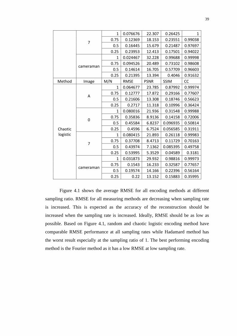
Figure 4.1 shows the average RMSE for all encoding methods at different

sampling ratio. RMSE for all measuring methods are decreasing when sampling rate

is increased. This is expected as the accuracy of the reconstruction should be

increased when the sampling rate is increased. Ideally, RMSE should be as low as

possible. Based on Figure 4.1, random and chaotic logistic encoding method have

comparable RMSE performance at all sampling rates while Hadamard method has

the worst result especially at the sampling ratio of 1. The best performing encoding

method is the Fourier method as it has a low RMSE at low sampling rate.

40

Figure 4.1: Average RMSE of all reconstructed images at different sampling ratio

Figure 4.2 shows the average PSNR for all encoding methods at different

sampling ratio. The higher the PSNR, the better the reconstruction image is. In terms

of PSNR, the performance has a similar trend as RMSE where random and chaotic

logistic method has average performance, Fourier method has the best performance

while Hadamard method has the worst performance.

Figure 4.2: Average PSNR of all reconstructed images at different sampling ratio

Figure 4.3 shows the average SSIM for all encoding methods at different

sampling ratio. SSIM is a perceptual metric that measures the structural similarity of

the image with respect to the original image. SSIM ranges from 0 to 1, with 1 being

0

0.05

0.1

0.15

0.2

0.25

0.3

0.35

0.4

0 0.2 0.4 0.6 0.8 1 1.2

M/N ratio

Average RMSE

Hadamard

random

Fourier

chaotic

0

5

10

15

20

25

30

0 0.2 0.4 0.6 0.8 1 1.2

M/N ratio

Average PSNR

Hadamard

random

Fourier

chaotic

41

the ideal value. The trend of the quality of the reconstructed image is similar to the

ones for RMSE and PSNR. The SSIM of Hadamard method is very low across all

sampling ratio, and performs the worst in this metric.

Figure 4.3: Average SSIM of all reconstructed images at different sampling ratio

Figure 4.3 shows the average CC for all encoding methods at different

sampling ratio. CC measures the relationship between two images. Value of CC

ranges from 0 to 1 where 1 is the best. Fourier performs the best at all sampling ratio

in this metric. The second-best performing encoding method is the random method.

Overall, chaotic logistic method has better CC than Hadamard method. However,

Hadamard method outperforms the chaotic logistic method at lower sampling ratios,

and even outperform the random method at sampling ratio of 0.25. The Hadamard

method has better performance when measured in this metric when compared with

RMSE, PSNR, and SSIM.

0

0.1

0.2

0.3

0.4

0.5

0.6

0.7

0 0.2 0.4 0.6 0.8 1 1.2

M/N ratio

Average SSIM

Hadamard

random

Fourier

chaotic

42

Figure 4.4: Average CC of all reconstructed images at different sampling ratio

After going through all the performance metrics for the encoding methods,

Fourier method has the best overall performance, followed by random method and

chaotic logistic method. The clear worst performer is the Hadamard method. This is

consistent with the result of the visual evaluation done in section 4.2. However, do

note that the performance of random and chaotic logistic method may fluctuate a

little depending on the seed used.

4.2.2 Security

The security tests done in this project are the histogram analysis, key space analysis,

and differential attack analysis. The security measurement metric values of all

encoding methods studied are tabulated in Table 4.6. The security is measured for

sampling ratio of 1 only because different sampling ratio is insignificant to the

security measurements metrics as the results are similar.

0

0.2

0.4

0.6

0.8

1

1.2

0 0.2 0.4 0.6 0.8 1 1.2

M/N ratio

Average CC

Hadamard

random

Fourier

chaotic

43

Table 4.6: Security measurement metric values of all encoding methods

Method Image M/N Histogram variance

NPCR UACI Key space

Hadamard

A

1

5.96 × 104 1.269531 0.004979

40964096 0 5.30 × 104 1.953125 0.007659

7 5.47 × 104 1.733398 0.006798

cameraman 4.31 × 104 3.466797 0.013595

random

A

1

3.65 × 104 2.246094 0.008808

24096×4096 0 2.35 × 104 3.369141 0.013212

7 2.87 × 104 2.758789 0.010819

cameraman 1.71 × 104 0.976563 0.00383

Fourier

A

1

5.93 × 104 0.90332 0.003542

1 0 5.37 × 104 2.001953 0.007851

7 5.55 × 104 1.464844 0.005744

cameraman 4.09 × 104 3.515625 0.013787

chaotic

A

1

5.52 × 104 2.978516 0.01168

3 × 1031 0 4.32 × 104 4.125977 0.018095

7 4.58 × 104 4.614258 0.018095

cameraman 2.93 × 104 2.001953 0.007851

First, results of histogram analysis will be evaluated. As observed from the

histograms in Figure 4.5, 4.6, 4.7, and 4.8, the ciphertext has intensity that is

concentrated on a certain value. Besides that, the concentration tends to follow a

similar pattern as the plaintext. The variance of all the histograms is in the order of

104, which indicates that the histogram is very concentrated around a few values only.

This shows the weakness in the security of SPI encoding as attacker can get clues on

the key and plaintext based on the concentrated values. The ideal histogram is evenly

distributed and different from the histogram of the plaintext. None of these methods

on any images provides a safe encryption in terms of histogram analysis. The

purpose of proposing a new method is to solve this problem.

44

Figure 4.5: Histogram of ciphertext and plaintext when using Hadamard method for

image: (a) A, (b) 0, (c) 7, (d) cameraman

(a)

(a)

(a)

(a)

(b)

(b)

(b)

(b)

(c)

(c)

(c)

(c)

(d)

(d)

(d)

(d)

45

Figure 4.6: Histogram of ciphertext and plaintext when using random method for

image: (a) A, (b) 0, (c) 7, (d) cameraman

(a)

(a)

(a)

(a)

(b)

(b)

(b)

(b)

(c)

(c)

(c)

(c)

(d)

(d)

(d)

(d)

46

Figure 4.7: Histogram of ciphertext and plaintext when using Fourier method for

image: (a) A, (b) 0, (c) 7, (d) cameraman

(a)

(a)

(a)

(a)

(c)

(c)

(c)

(c)

(d)

(d)

(d)

(d)

(b)

(b)

(b)

(b)

47

Figure 4.8: Histogram of ciphertext and plaintext when using chaotic logistic method

for image: (a) A, (b) 0, (c) 7, (d) cameraman

Next, the results of differential attack analysis are discussed. For the

encryption to be good against differential attack, its NPCR and UACI should be

close to 99.6094070 and 33.463507 respectively (Liu and Ding, 2020). Based on

Table 4.6, all the methods on all images produces NPCR and UACI values that are

very low and far from the ideal value. This low value indicates that when the

plaintext is changed slightly, the ciphertext will only have a very slight change. This

is a bad situation for security as attackers can accumulate clues after many iterations.

Now, the key space analysis will be discussed. Key space of an encoding

method is the same for all images. The calculation of key space will depend on the

encoding method. For the Hadamard method, since M Hadamard masks is arranged

randomly, the key space will be MM, where M is the number of sampling

measurements. In this project, number of pixels N is set to 4096, thus the key space

for Hadamard method for sampling ratio of 1 is 40964096. Next, key space calculation

for random method is evaluated. Since values in the measurement matrix are bipolar

and there are 𝑀 × 𝑁 number of elements, the key space for random method when the

(a)

(a)

(a)

(a)

(b)

(b)

(b)

(b)

(c)

(c)

(c)

(c)

(d)

(d)

(d)

(d)

48

sampling ratio is 1 is 24096×4096. Next, the key space for Fourier method is only one

since the Fourier map is used as it is for the encoding. For chaotic logistic method,

there are two element that dictates the map, which is the initial condition that ranges

from 0 to 1 and the growth rate that ranges from 3.7 to 4. Assuming the computer has

a precision of 10-16, the key space will be 1016 × 1016 × 0.3 = 3 × 1031.

The size of key space for all encoding methods except Fourier method meets

the minimum size to be considered robust which is 1030. The key space of Hadamard

and random method may seem extremely large but in reality, it is actually smaller.

The calculation assumes that random number generation in MATLAB is truly

random when in reality it is not. The random number generation in MATLAB is

pseudorandom and depend on some algorithm and seed which has smaller key space

than the key space calculated here.

In summary, the security of available SPI encoding method is not enough as

there are some drawbacks such as concentrated histogram and vulnerable to

differential attack.

4.3 Comparisons Between Proposed Method

Two methods have been proposed to improve the security of the SPI encoding

scheme. They are the mixed logistic map SPI-DRPE and mixed logistic map SPI-

RSA. They will be mentioned as SPI-DRPE and SPI-RSA in this section. Their

reconstruction quality and security will be compared.

4.3.1 Reconstruction Quality

Table 4.7 shows the tabulated reconstruction quality measurement metrics for all

tested images. From Table 4.7, we can observe that the value of all the quality

measurement metrics is the same for all the images and sampling ratios. This is

because the second phase encryption, DRPE and RSA returns perfect results when

decryption is done. Thus, the part that is actually evaluated is the first phase

encryption, which is the same for both methods.

49

Table 4.7: Quality metrics for SPI-DRPE and SPI-RSA

Method Image M/N RMSE PSNR SSIM CC

SPI-DRPE

A

1 0.061144 24.273 0.89434 0.99971

0.75 0.18623 14.599 0.27264 0.76519

0.5 0.24394 12.254 0.17833 0.58183

0.25 0.27833 11.109 0.11665 0.37295

0

1 0.074794 22.523 0.31931 0.99987

0.75 0.36545 8.7434 0.14003 0.71758

0.5 0.43895 7.1517 0.10301 0.51739

0.25 0.48464 6.2916 0.060181 0.3323

7

1 0.078934 22.055 0.26218 0.99983

0.75 0.37735 8.4651 0.11591 0.7124

0.5 0.39017 8.175 0.081261 0.50318

0.25 0.52503 5.5963 0.043772 0.29502

cameraman

1 0.030737 30.247 0.98832 0.99974

0.75 0.16091 15.868 0.33319 0.77954

0.5 0.19661 14.128 0.23415 0.57045

0.25 0.25633 11.824 0.16569 0.35731

SPI-RSA

A

1 0.061144 24.273 0.89434 0.99971

0.75 0.18623 14.599 0.27264 0.76519

0.5 0.24394 12.254 0.17833 0.58183

0.25 0.27833 11.109 0.11665 0.37295

0

1 0.074794 22.523 0.31931 0.99987

0.75 0.36545 8.7434 0.14003 0.71758

0.5 0.43895 7.1517 0.10301 0.51739

0.25 0.48464 6.2916 0.060181 0.3323

7

1 0.078934 22.055 0.26218 0.99983

0.75 0.37735 8.4651 0.11591 0.7124

0.5 0.39017 8.175 0.081261 0.50318

0.25 0.52503 5.5963 0.043772 0.29502

cameraman

1 0.030737 30.247 0.98832 0.99974

0.75 0.16091 15.868 0.33319 0.77954

0.5 0.19661 14.128 0.23415 0.57045

0.25 0.25633 11.824 0.16569 0.35731

4.3.2 Security

The security analysis done are the histogram analysis, differential attack analysis,

and key space analysis. The security analysis is done only for sampling ratio of 1

because the security analysis for different sampling ratio is redundant.

50

Table 4.8: Results of security analysis

Method Image M/N Histogram variance

NPCR UACI Key space

SPI-DRPE

A

1

8.97E+02 3.686523 0.014457 2.7 ×1094 (first

phase),

(40961016)2

(second phase)

0 1.17E+03 3.735352 0.014648

7 1.79E+03 3.881836 0.015223

cameraman 2.40E+02 1.318359 0.00517

SPI-RSA

A

1

1.40E+02 100 47.10445

2.7 × 1094 (first phase)

0 1.23E+02 100 47.89199

7 1.77E+02 100 48.69221

cameraman 1.29E+02 100 47.35618

First, histogram analysis is discussed. Figure 4.9 and 4.10 shows the

histogram of the final ciphertext and plaintext of all images for SPI-DRPE and SPI-

RSA respectively at sampling ratio of 1. For SPI-DRPE, it is observed that the

histogram of final ciphertext is slightly spread out compared to the histogram of

conventional SPI encoding. However, it still slightly resembles the original image

histogram and is still too focused on one spot. The average variance of the histogram

is still high with a value of 1030. For SPI-RSA, the histograms of the final ciphertext

are spread out over the intensity spectrum. Although the histograms do not appear

uniform, they do not resemble the original image histogram. The average variance of

the histogram is 140 which is low compared to SPI-DRPE. This means that the

histogram of SPI-RSA is more spread out compared to SPI-DRPE. Therefore, SPI-

RSA is more secure compared to SPI-DRPE when analysed with histogram as it is

harder to derive any clues from the histogram of SPI-RSA compared with SPI-DRPE.

51

Figure 4.9: Histogram of final ciphertext and plaintext when using SPI-DRPE

method for image: (a) A, (b) 0, (c) 7, (d) cameraman

(a)

(a)

(a)

(a)

(b)

(b)

(b)

(b)

(c)

(c)

(c)

(c)

(d)

(d)

(d)

(d)

52

Figure 4.10: Histogram of final ciphertext and plaintext when using SPI-RSA

method for image: (a) A, (b) 0, (c) 7, (d) cameraman

Next, differential attack analysis is discussed. For the encryption to be good

against differential attack, its NPCR and UACI should be close to 99.6094070 and

33.463507 respectively (Liu and Ding, 2020). Higher value of NPCR and UACI is

better. Based on Table 4.8, the NPCR and UACI of SPI-DRPE is still low and not

close to the ideal value. This means that there is only a little change in the final

ciphertext when one pixel of plaintext is altered. On the other hand, SPI-RSA boasts

an average NPCR and UACI of 100 and 47.8 respectively. They are closer to the

ideal value and higher. NPCR of 100 means that all the pixels in the final ciphertext

will change when one pixel of the plaintext is altered. Thus, SPI-RSA is very

resistant to differential attack, unlike its SPI-DRPE counterpart.

Finally, the key space analysis is discussed. Assume the precision of the

computer is up to 10-16. For the first phase encryption, the key space is calculated as

(1016 × 1016 × 0.3)3 = 2.7 × 1094 . The calculation is done so because there are

three logistic maps used in this encryption and the key space of one logistic map is

1016 × 1016 × 0.3. The key space of the second phase encryption for SPI-DRPE at

(a)

(a)

(a)

(a)

(b)

(b)

(b)

(b)

(c)

(c)

(c)

(c)

(d)

(d)

(d)

(d)

53

the sampling ratio of 1 is calculated as (40961016)2 . This is because there are 2

random number arrays created to form RP1 and RP2. and the random number ranges

from 0 to 1 with precision assumed to be 10-16. 4096 is the number of pixels of the

first ciphertext when sampling ratio is 1. The key space of the second phase

encryption for SPI-RSA is hard to find because the key space of asymmetric

cryptosystem is less studied, thus it is not discussed here. The total key space of the

proposed systems is found by adding phase 1 and phase 2 key space. The phase 2 key

space of DRPE is extremely large, though in reality it is smaller due to the random

number generator being not truly random. The key space of the first phase alone is

2.7 × 1094 which is much larger than 1030. This makes both proposed method a

robust encryption method against brute force attacks.

4.4 Overall Comparisons

The proposed methods are compared with the conventional SPI encoding methods.

The SPI encoding method chosen to be compared with the proposed methods are the

chaotic logistic method and Fourier method. Chaotic logistic method is chosen

because the first phase of the proposed methods is derived from the logistic map.

Fourier method is chosen because it has the best quality performance out of all of the

studied SPI encoding methods. First, visual evaluation is done based on Table 4.9,

4.10, 4.11, and 4.12.

Table 4.9: Reconstructed images for image A

Sampling ratio

(M/N)

0.25 0.5 0.75 1

Original image

Reconstructed

image

(Fourier)

54

Table 4.10: Reconstructed images for image 0

Reconstructed

image (Chaotic

logistic)

Reconstructed

image (SPI-

DRPE and SPI-

RSA)

Sampling ratio

(M/N)

0.25 0.5 0.75 1

Original image

Reconstructed

image

(Fourier)

Reconstructed

image (Chaotic

logistic)

Reconstructed

image (SPI-

DRPE and SPI-

RSA)

55

Table 4.11: Reconstructed images for image 7

Table 4.12: Reconstructed images for image cameraman

Sampling ratio

(M/N)

0.25 0.5 0.75 1

Original image

Reconstructed

image

(Fourier)

Reconstructed

image (Chaotic

logistic)

Reconstructed

image (SPI-

DRPE and SPI-

RSA)

Sampling ratio

(M/N)

0.25 0.5 0.75 1

Original image

Reconstructed

image

(Fourier)

56

The method that produces the reconstruction quality visually is the Fourier

method. The proposed methods and the chaotic logistic method look extremely

similar.

Next, we will evaluate the quality quantitatively. The average RMSE, PSNR,

SSIM, and CC for the studied methods are plotted against the sampling ratio in

Figure 4.11, 4.12, 4.13, and 4.14. The quality evaluation metrics shows an improving

trend when sampling ratio is increased. The Fourier method reigns superior in terms

of reconstruction quality for all metrics at low sampling rate. Chaotic logistic method

has similar quality performance across the board with the proposed methods. This

trend matches the visual evaluation.

Figure 4.11: Average RMSE for different sampling ratio

0

0.05

0.1

0.15

0.2

0.25

0.3

0.35

0.4

0.45

0 0.2 0.4 0.6 0.8 1 1.2

M/N ratio

Average RMSE

Fourier

chaotic

proposed

Reconstructed

image (Chaotic

logistic)

Reconstructed

image (SPI-

DRPE and SPI-

RSA)

57

Figure 4.12: Average PSNR for different sampling ratio

Figure 4.13: Average SSIM for different sampling ratio

0

5

10

15

20

25

30

0 0.2 0.4 0.6 0.8 1 1.2

M/N ratio

Average PSNR

Fourier

chaotic

proposed

0

0.1

0.2

0.3

0.4

0.5

0.6

0.7

0 0.2 0.4 0.6 0.8 1 1.2

M/N ratio

Average SSIM

Fourier

chaotic

proposed

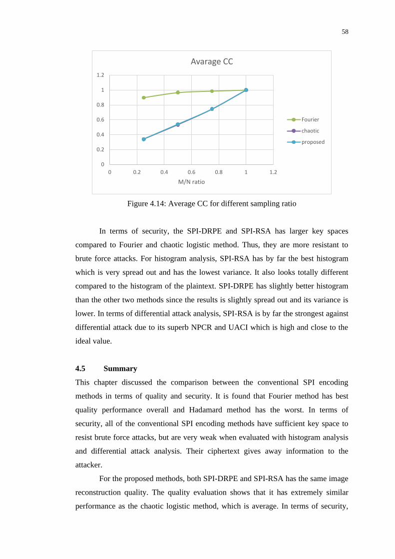
58

Figure 4.14: Average CC for different sampling ratio

In terms of security, the SPI-DRPE and SPI-RSA has larger key spaces

compared to Fourier and chaotic logistic method. Thus, they are more resistant to

brute force attacks. For histogram analysis, SPI-RSA has by far the best histogram

which is very spread out and has the lowest variance. It also looks totally different

compared to the histogram of the plaintext. SPI-DRPE has slightly better histogram

than the other two methods since the results is slightly spread out and its variance is

lower. In terms of differential attack analysis, SPI-RSA is by far the strongest against

differential attack due to its superb NPCR and UACI which is high and close to the

ideal value.

4.5 Summary

This chapter discussed the comparison between the conventional SPI encoding

methods in terms of quality and security. It is found that Fourier method has best

quality performance overall and Hadamard method has the worst. In terms of

security, all of the conventional SPI encoding methods have sufficient key space to

resist brute force attacks, but are very weak when evaluated with histogram analysis

and differential attack analysis. Their ciphertext gives away information to the

attacker.

For the proposed methods, both SPI-DRPE and SPI-RSA has the same image

reconstruction quality. The quality evaluation shows that it has extremely similar

performance as the chaotic logistic method, which is average. In terms of security,

0

0.2

0.4

0.6

0.8

1

1.2

0 0.2 0.4 0.6 0.8 1 1.2

M/N ratio

Avarage CC

Fourier

chaotic

proposed

59

SPI-RSA is the best with good histogram spread that does not give away information,

lowest histogram variance, great resistance against differential attack and very good

resistance against brute force attack. SPI-DRPE method is inferior in every way

when compared with SPI-RSA except the key space. Its security is a slight

improvement compared with the conventional SPI encoding methods in this study.

Thus, SPI-RSA is a very good foundation for better SPI based encryption framework.

60

CHAPTER 5

5 CONCLUSIONS AND RECOMMENDATIONS

5.1 Conclusions

In this project, many SPI and non-SPI encoding and decoding schemes are reviewed.

The reviewed SPI encoding and decoding strengthened the foundation in order to

develop a better encoding scheme. The analysis of DRPE and RSA encryption

framework have helped in developing the proposed SPI based encryption method

that are more secure.

A novel encryption method based on SPI is successfully developed and have

overcome the security problems of SPI encoding using the knowledge of DRPE,

RSA and chaotic theory.

Besides, the performance of the designed method and available SPI based

encoding method are evaluated based on its quality and security using quantifiable

metrics. The designed method is also compared with the available SPI encoding

method. Through the comparisons, the strengths and weaknesses of the proposed

method are found. It is found that the proposed mixed logistic map SPI-RSA has

greatly improved the security of the SPI encoding method.

5.2 Recommendations for future work

The proposed methods, namely mixed logistic map SPI-DRPE and SPI-RSA

encryption framework can be further improved, especially the SPI-DRPE method.

For instance, the first ciphertext can be padded in order to get a more uniform

histogram distribution.

Since this project is done through simulation using MATLAB, it is hoped that

this project can be done physically so that the implication of real-world conditions

such as noise on the proposed methods can be studied. One of the suggestions is that

a DMD can be used as the light pattern modulator of the SPI setup.

The encryption and decryption time analysis of the proposed methods can be

done in the future as time is a very important factor when encryption and decryption

need to be done in real time. However, there is a limitation on the proposed method

in terms of encryption and decryption time. Since the proposed method is a double

61

encryption, two encryption processes need to be done in order to encrypt an image.

This will usually take more time compared to a conventional SPI encoding method

that only encodes the image one time only. A smarter approach is needed in order to

reduce or fully overcome this limitation.

It is hoped that the proposed mixed logistic map SPI-RSA can be a starting

point in inspiring the development of more secure and robust SPI based encoding

methods.

62

REFERENCES

Agarwal, S., 2018. A Review of Image Scrambling Technique Using Chaotic Maps.

International Journal of Engineering and Technology Innovation, 8(2), pp. 77–98.

Alfalou, A. and Brosseau, C., 2009. Optical image compression and encryption

methods. Advances in Optics and Photonics, [e-journal] 1(3), p. 589–589.

http://dx.doi.org/10.1364/AOP.1.000589.

Alfalou, A. and Mansour, A., 2009. A new double random phase encryption scheme

to multiplex and simultaneous encode multiple images. Applied optics, Optical

Society of America, 48(31), pp. 5933–5947. <https://hal.archives-ouvertes.fr/hal-

00579204> [Accessed 9 March 2020].

Boeing, G., 2016. Visual Analysis of Nonlinear Dynamical Systems: Chaos, Fractals,

Self-Similarity and the Limits of Prediction. Systems, [e-journal] 4(4), p. 37–37.

http://dx.doi.org/10.3390/systems4040037.

Donoho, D. L., 2006. Compressed sensing. IEEE Transactions on Information

Theory, 52(4), 1289-1306. IEEE Transactions on Information Theory, [e-journal]

52(4), pp. 1289–1306. http://dx.doi.org/10.1109/TIT.2006.871582.

Edgar, M. P., Gibson, G. M. and Padgett, M. J., 2019. Principles and prospects for

single-pixel imaging. Nature Photonics, [e-journal] 13(1), pp. 13–20.

http://dx.doi.org/10.1038/s41566-018-0300-7.

Glückstad, J. and Palima, D., 2009. Generalized phase contrast: Applications in

optics and photonics / Jesper Glückstad, Darwin Palima. [e-book]. Dordrecht,

Bristol: Springer in association with Canopus Academic Pub.

<http://www.springer.com/gb/ BLDSS> [Accessed 28 August 2020].

Glückstad, J. and Palima, D., 2009. Optical Encryption and Decryption. In: 2009.

Generalized phase contrast. Applications in optics and photonics / Jesper Glückstad,

Darwin Palima. Dordrecht, Bristol: Springer in association with Canopus Academic

Pub, pp. 273–298.

Heucheun Yepdia, L. M., Tiedeu, A. and Kom, G., 2021. A Robust and Fast Image

Encryption Scheme Based on a Mixing Technique. Security and Communication

Networks, [e-journal] 2021, pp. 1–17. http://dx.doi.org/10.1155/2021/6615708.

63

Jiao, K., Ye, G., Dong, Y., Huang, X. and He, J., 2020. Image Encryption Scheme

Based on a Generalized Arnold Map and RSA Algorithm. Security and

Communication Networks, [e-journal] 2020, pp. 1–14.

http://dx.doi.org/10.1155/2020/9721675.

Jiao, S., Lei, T., Gao, Y., Xie, Z. and Yuan, X., 2019. Known-Plaintext Attack and

Ciphertext-Only Attack for Encrypted Single-Pixel Imaging. IEEE Access, 7,

119557-119565. IEEE Access, [e-journal] 7, pp. 119557–119565.

http://dx.doi.org/10.1109/ACCESS.2019.2936119.

Liu, C. and Ding, Q., 2020. A Color Image Encryption Scheme Based on a Novel 3D

Chaotic Mapping. Complexity, [e-journal] 2020, pp. 1–20.

http://dx.doi.org/10.1155/2020/3837209.

Liu, S., Guo, C. and Sheridan, J. T., 2014. A review of optical image encryption

techniques. Optics & Laser Technology, [e-journal] 57, pp. 327–342.

http://dx.doi.org/10.1016/j.optlastec.2013.05.023.

Padgett, M. J. and Boyd, R. W., 2017. An introduction to ghost imaging: quantum

and classical. Philosophical transactions. Series A, Mathematical, physical, and

engineering sciences, [e-journal] 375(2099).

http://dx.doi.org/10.1098/rsta.2016.0233.

Rani, M., Dhok, S. B. and Deshmukh, R. B., 2018. A Systematic Review of

Compressive Sensing: Concepts, Implementations and Applications. IEEE Access, 6,

4875-4894. IEEE Access, [e-journal] 6, pp. 4875–4894.

http://dx.doi.org/10.1109/ACCESS.2018.2793851.

Xiong, R., Zhang, L., Pan, Z., Zhang, D., Wang, Z. and Wang, K., 2020.

Performance comparison based on single-pixel imaging methods in the time domain.

Laser Physics, [e-journal] 30(1), p. 15202–15202. http://dx.doi.org/10.1088/1555-

6611/ab4bba.

Zhang, C., Han, B., He, W., Peng, X. and Xu, C., 2019. A Novel Compressive

Optical Encryption via Single-Pixel Imaging. IEEE Photonics Journal, [e-journal]

11(4), pp. 1–8. http://dx.doi.org/10.1109/JPHOT.2019.2924457.

64

Zhang, C., He, W., Han, B., Liao, M., Lu, D., Peng, X. and Xu, C., 2019.

Compressive optical steganography via single-pixel imaging. Optics express, [e-

journal] 27(9), pp. 13469–13478. http://dx.doi.org/10.1364/OE.27.013469.

Zhao, G., Yang, X., Zhou, B. and Wei, W., 2010. RSA-based digital image

encryption algorithm in wireless sensor networks. In: ICSPS 2010. 2010 2nd

International Conference on Signal Processing Systems : 5-7 July 2010, Dalian,

China : Proceedings. 2010 2nd International Conference on Signal Processing

Systems (ICSPS). Dalian, China, 7/5/2010 - 7/7/2010. Piscataway, N.J.: IEEE, V2-

640-V2-643.

Zhou, X. and Tang, X., 2011. Research and implementation of RSA algorithm for

encryption and decryption. In: Proceedings of the 6th International Forum on

Strategic Technology. August 22-24, 2011, Harbin, China. 2011 6th International

Forum on Strategic Technology (IFOST). Harbin, Heilongjiang, China, 8/22/2011 -

8/24/2011. Piscataway, NJ: IEEE, pp. 1118–1121.

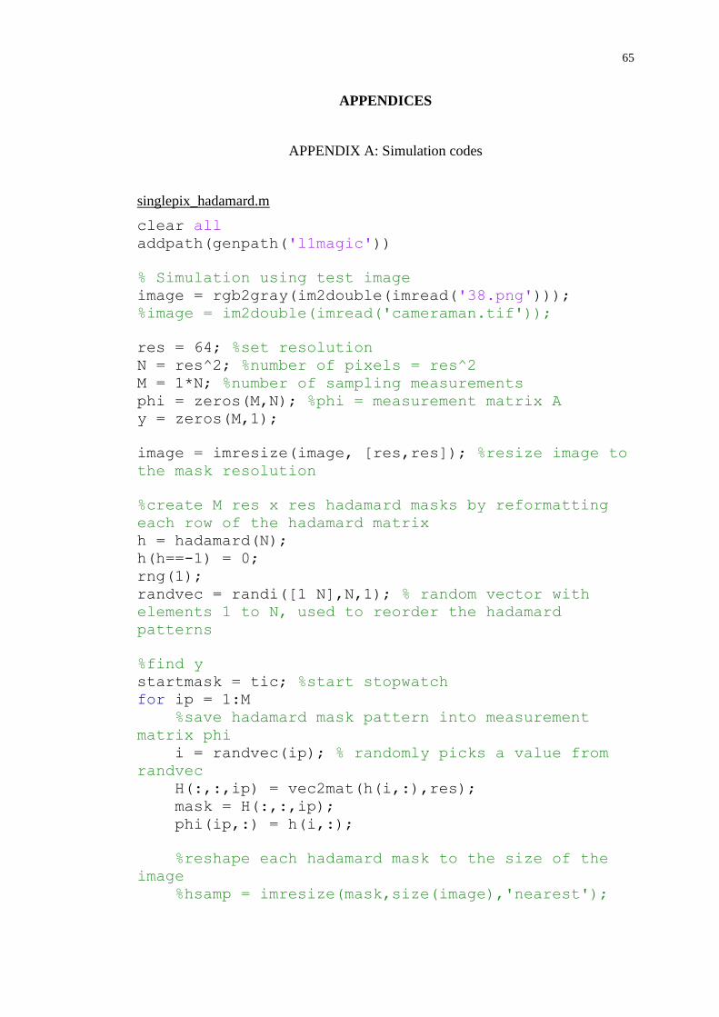
65

APPENDICES

APPENDIX A: Simulation codes

singlepix_hadamard.m

clear all

addpath(genpath('l1magic'))

% Simulation using test image

image = rgb2gray(im2double(imread('38.png')));

%image = im2double(imread('cameraman.tif'));

res = 64; %set resolution

N = res^2; %number of pixels = res^2

M = 1*N; %number of sampling measurements

phi = zeros(M,N); %phi = measurement matrix A

y = zeros(M,1);

image = imresize(image, [res,res]); %resize image to

the mask resolution

%create M res x res hadamard masks by reformatting

each row of the hadamard matrix

h = hadamard(N);

h(h==-1) = 0;

rng(1);

randvec = randi([1 N],N,1); % random vector with

elements 1 to N, used to reorder the hadamard

patterns

%find y

startmask = tic; %start stopwatch

for ip = 1:M

%save hadamard mask pattern into measurement

matrix phi

i = randvec(ip); % randomly picks a value from

randvec

H(:,:,ip) = vec2mat(h(i,:),res);

mask = H(:,:,ip);

phi(ip,:) = h(i,:);

%reshape each hadamard mask to the size of the

image

%hsamp = imresize(mask,size(image),'nearest');

66

hsamp = mask;

%project pattern sequence to image

temp = image;

temp(hsamp==0) = 0;

%record average intensity

y(ip) = sum(sum(temp))./numel(temp);

end

endmask = toc(startmask); %stop stopwatch and record

the reading time

%solve and reconstruct image

% Find x, image represention --> estIm

% y = Ax

% x = A-1*y = A\y --> inverse A

% Note: x = img0/estIm (Nx1), A = phi (MxN), y =

aver (Mx1)

startrecon = tic; %start stopwatch

invphi = pinv(phi);%pinv(A) returns the Moore-

Penrose Pseudoinverse of matrix A.

im0 = invphi*y;%initial solution, im0 = x, y = phi*x,

x = (phi^-1)*y

estIm = l1dantzig_pd(im0, phi, [], y, 0.01, 1e-4,2);

% Reconstruct image

reconIm = vec2mat(estIm,res);

reconIm = (reconIm-

min(min(reconIm)))/(max(max(reconIm))-

min(min(reconIm)));%normalize image

endrecon = toc(startrecon); %end stopwatch and

record reconstruction time

%calculate RMSE

A = zeros(res,res);

scaled_image = imresize(image,size(A));

o = vec2mat(scaled_image,1);

o_un = vec2mat(reconIm,1);

for i = 1:N

diff = (o_un(i,1) - o(i,1));

diff_sq(i,:) = diff^2;

end

diff_sq_sum = sum(diff_sq,1);

RMSE = sqrt(diff_sq_sum/N);

%calculate PSNR

67

peaksnr = psnr(reconIm, scaled_image);

%calculate SSIM

ssimval = ssim(reconIm, scaled_image);

%calculate CC

ccval = corr2(scaled_image, reconIm);

%calculate M/N

MNratio = M/N;

%show the rescaled image

figure;

subplot(1,2,1); imshow(scaled_image);

title('Rescaled image');

%show the reconstructed image

subplot(1,2,2); imshow(reconIm);

title(['Reconstructed image']);

%Security analysis

%histogram analysis

figure; subplot(1,2,1);

imhist(y); title('histogram of y');

[ycounts, ybinLocations] = imhist(y);

subplot(1,2,2);

imhist(scaled_image); title('histogram of image');

[imcounts, imbinLocations] = imhist(scaled_image);%

title('histogram of image');

%image entropy

y_entropy = entropy(y);

%histogram variance

imdata=reshape(transpose(scaled_image),1,[]);

v = var(ycounts);

vim = var(imcounts);

%differential attack analysis: NPCR & UACI

img_chg = image;

img_chg(1,1) = 1;

y_chg = zeros(M,1);

for ip = 1:M

mask = H(:,:,ip);

hsamp = mask;

68

%project pattern sequence to image

temp = img_chg;

temp(hsamp==0) = 0;

%record average intensity

y_chg(ip) = sum(sum(temp))./numel(temp);

end

y = round(255.*y);

y_chg = round(255.*y_chg);

D = 0;

diffsum = 0;

for i=1:M

if(y(i)~=y_chg(i))

D = D + 1;

end

diffsum = diffsum + abs(y(i) - y_chg(i))/255;

end

NPCR = (D/M)*100;

UACI = 100*diffsum/M;

%tabulate results

T = table(MNratio, RMSE, peaksnr, ssimval, ccval,

endmask, endrecon);

disp(T);

singlepix_random.m

clear all

addpath(genpath('l1magic'))

% Simulation using test image

image = rgb2gray(im2double(imread('192.png')));

%image = im2double(imread('A.png'));

res = 64; %set resolution

N = res^2; %number of pixels = res^2

M = 1*N; %number of sampling measurements

phi = zeros(M,N); %phi = measurement matrix A

y = zeros(M,1);

image = imresize(image, [res,res]); %resize image to

the mask resolution

% Find y, measurement --> average intensity

startmask = tic; %start stopwatch

for ip = 1:M

69

rng(ip); %fix the random seed

randp = randi([0 1],res); %binary pattern generated

(sqrt(N)xsqrt(N))

%randsamp =

imresize(randp,size(image),'nearest'); %resize

pattern to image resolution

randsamp = randp;

phi(ip,:) = randp(:)';%save pattern (sqrt(N)xsqrt(N))

into sampling matrix (MxN)

%project pattern sequence to image (keep only

datapoints from on pixels)

temp = image;

temp(randsamp==0) = 0;

%get average intensity

y(ip) = sum(sum(temp))./numel(temp);

end

endmask = toc(startmask); %stop stopwatch and record

the reading time

%solve and reconstruct image

% Find x, image represention --> estIm

% y = Ax

% x = A-1*y = A\y --> inverse A

% Note: x = img0/estIm (Nx1), A = phi (MxN), y =

aver (Mx1)

startrecon = tic; %start stopwatch

invphi = pinv(phi);%pinv(A) returns the Moore-

Penrose Pseudoinverse of matrix A.

im0 = invphi*y;%initial solution, im0 = x, y = phi*x,

x = (phi^-1)*y

estIm = l1dantzig_pd(im0, phi, [], y, 0.01, 1e-4,2);

% Reconstruct image

reconIm = reshape(estIm,res,res);

reconIm = (reconIm-

min(min(reconIm)))/(max(max(reconIm))-

min(min(reconIm)));%normalize image

endrecon = toc(startrecon); %end stopwatch and

record reconstruction time

%calculate RMSE

A = zeros(res,res);

scaled_image = imresize(image,size(A));

70

o = vec2mat(scaled_image,1);

o_un = vec2mat(reconIm,1);

for i = 1:N

diff = (o_un(i,1) - o(i,1));

diff_sq(i,:) = diff^2;

end

diff_sq_sum = sum(diff_sq,1);

RMSE = sqrt(diff_sq_sum/N);

%calculate PSNR

peaksnr = psnr(reconIm, scaled_image);

%calculate SSIM

ssimval = ssim(reconIm, scaled_image);

%calculate CC

ccval = corr2(scaled_image, reconIm);

%calculate M/N

MNratio = M/N;

y_entropy = entropy(y);

%show the rescaled image

figure;

subplot(1,2,1); imshow(scaled_image);

title('Rescaled image');

%show the reconstructed image

subplot(1,2,2); imshow(reconIm);

title(['Reconstructed image']);

%Security analysis

%histogram analysis

figure; subplot(1,2,1);

imhist(y); title('histogram of y');

[ycounts, ybinLocations] = imhist(y);

subplot(1,2,2);

imhist(scaled_image); title('histogram of image');

[imcounts, imbinLocations] = imhist(scaled_image);%

title('histogram of image');

%image entropy

y_entropy = entropy(y);

%histogram variance

imdata=reshape(transpose(scaled_image),1,[]);

71

v = var(ycounts);

vim = var(imcounts);

%differential attack analysis: NPCR & UACI

img_chg = image;

img_chg(1,1) = 1;

y_chg = zeros(M,1);

for ip = 1:M

rng(ip); %fix the random seed

mask = randi([0 1],res);

randsamp = mask;

%project pattern sequence to image

temp = img_chg;

temp(randsamp==0) = 0;

%record average intensity

y_chg(ip) = sum(sum(temp))./numel(temp);

end

y = round(255.*y);

y_chg = round(255.*y_chg);

D = 0;

diffsum = 0;

for i=1:M

if(y(i)~=y_chg(i))

D = D + 1;

end

diffsum = diffsum + abs(y(i) - y_chg(i))/255;

end

NPCR = (D/M)*100;

UACI = 100*diffsum/M;

%tabulate results

T = table(MNratio, RMSE, peaksnr, ssimval, ccval,

endmask, endrecon);

disp(T);

singlepix_fourier.m

clear all

addpath(genpath('l1magic'))

% Simulation using test image

%image = rgb2gray(im2double(imread('192.png')));

image = im2double(imread('cameraman.tif'));

72

res = 64; %set resolution

N = res^2; %number of pixels = res^2

M = 1*N; %number of sampling measurements

phi = zeros(M,N); %phi = measurement matrix A

y = zeros(M,1);

image = imresize(image, [res,res]); %resize image to

the mask resolution

%create N res x res Fourier masks by reformatting

each row of the DCT matrix

dct = dctmtx(N);

dct(dct<=0)=0;

dct(dct>0)=1;

%find y

startmask = tic; %start stopwatch

for ip = 1:M

%save Fourier mask pattern into measurement

matrix phi

H(:,:,ip) = vec2mat(dct(ip,:),res);

mask = H(:,:,ip);

phi(ip,:) = dct(ip,:);

%reshape each Fourier mask to the size of the

image

%dctsamp = imresize(mask,size(image),'nearest');

dctsamp = mask;

%project pattern sequence to image

temp = image;

temp(dctsamp==0) = 0;

%record average intensity

y(ip) = sum(sum(temp))./numel(temp);

end

endmask = toc(startmask); %stop stopwatch and record

the reading time

%y = round(255.*y)./255;

%solve and reconstruct image

% Find x, image represention --> estIm

% y = Ax

% x = A-1*y = A\y --> inverse A

% Note: x = img0/estIm (Nx1), A = phi (MxN), y =

aver (Mx1)

startrecon = tic; %start stopwatch

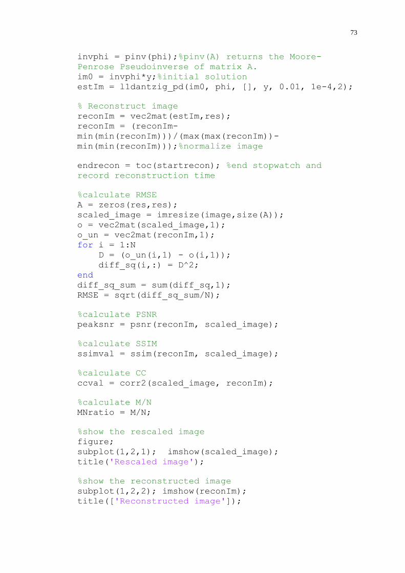
73

invphi = pinv(phi);%pinv(A) returns the Moore-

Penrose Pseudoinverse of matrix A.

im0 = invphi*y;%initial solution

estIm = l1dantzig_pd(im0, phi, [], y, 0.01, 1e-4,2);

% Reconstruct image

reconIm = vec2mat(estIm,res);

reconIm = (reconIm-

min(min(reconIm)))/(max(max(reconIm))-

min(min(reconIm)));%normalize image

endrecon = toc(startrecon); %end stopwatch and

record reconstruction time

%calculate RMSE

A = zeros(res,res);

scaled_image = imresize(image,size(A));

o = vec2mat(scaled_image,1);

o_un = vec2mat(reconIm,1);

for i = 1:N

D = (o_un(i,1) - o(i,1));

diff_sq(i,:) = D^2;

end

diff_sq_sum = sum(diff_sq,1);

RMSE = sqrt(diff_sq_sum/N);

%calculate PSNR

peaksnr = psnr(reconIm, scaled_image);

%calculate SSIM

ssimval = ssim(reconIm, scaled_image);

%calculate CC

ccval = corr2(scaled_image, reconIm);

%calculate M/N

MNratio = M/N;

%show the rescaled image

figure;

subplot(1,2,1); imshow(scaled_image);

title('Rescaled image');

%show the reconstructed image

subplot(1,2,2); imshow(reconIm);

title(['Reconstructed image']);

74

%Security analysis

%histogram analysis

figure; subplot(1,2,1);

imhist(y); title('histogram of y');

[ycounts, ybinLocations] = imhist(y);

subplot(1,2,2);

imhist(scaled_image); title('histogram of image');

[imcounts, imbinLocations] = imhist(scaled_image);%

title('histogram of image');

%image entropy

y_entropy = entropy(y);

%histogram variance

imdata=reshape(transpose(scaled_image),1,[]);

v = var(ycounts);

vim = var(imcounts);

%differential attack analysis: NPCR & UACI

img_chg = image;

img_chg(1,1) = 1;

y_chg = zeros(M,1);

for ip = 1:M

mask = H(:,:,ip);

dctsamp = mask;

%project pattern sequence to image

temp = img_chg;

temp(dctsamp==0) = 0;

%record average intensity

y_chg(ip) = sum(sum(temp))./numel(temp);

end

y = round(255.*y);

y_chg = round(255.*y_chg);

D = 0;

diffsum = 0;

for i=1:M

if(y(i)~=y_chg(i))

D = D + 1;

end

diffsum = diffsum + abs(y(i) - y_chg(i))/255;

end

NPCR = (D/M)*100;

UACI = 100*diffsum/M;

75

%tabulate results

T = table(MNratio, RMSE, peaksnr, ssimval, ccval,

endmask, endrecon);

disp(T);

singlepix_chaotic_logistic.m

clear all

addpath(genpath('l1magic'))

% Simulation using test image

image = rgb2gray(im2double(imread('192.png')));

%image = im2double(imread('cameraman.tif'));

res = 64; %set resolution

N = res^2; %number of pixels = res^2

M = 1*N; %number of sampling measurements

phi = zeros(M,N); %phi = measurement matrix A

y = zeros(M,1);

image = imresize(image, [res,res]); %resize image to

the mask resolution

%create M res x res chaotic masks by reformatting

the logistic map to matrix

r = 3.8; % r parameter for chaotic regime

csize = M*N; % size of chaotic array

x(1)= 0.4; % initial value

for i=1:csize-1

x(i+1) = r*x(i)*(1-x(i));

end

cmat=vec2mat(x, N);

cmat(cmat<0.5) = 0;

cmat(cmat>=0.5) = 1;

%find y

startmask = tic; %start stopwatch

for ip = 1:M

%arrange chaotic mask pattern into res x res

matrix

H(:,:,ip) = vec2mat(cmat(ip,:),res);

mask = H(:,:,ip);

%reshape each chaotic mask to the size of the

image

%csamp = imresize(mask,size(image),'nearest');

csamp = mask;

76

%project pattern sequence to image

temp = image;

temp(csamp==0) = 0;

%record average intensity

y(ip) = sum(sum(temp))./numel(temp);

end

endmask = toc(startmask); %stop stopwatch and record

the reading time

%solve and reconstruct image

% Find x, image represention --> estIm

% y = Ax

% x = A-1*y = A\y --> inverse A

% Note: x = img0/estIm (Nx1), A = phi (MxN), y =

aver (Mx1)

startrecon = tic; %start stopwatch

%get phi using correct seed

r = 3.8; % r parameter for chaotic regime

csize = M*N; % size of chaotic array

x(1)= 0.4; % initial value (seed)

for i=1:csize-1

x(i+1) = r*x(i)*(1-x(i));

end

cmat=vec2mat(x,N);

cmat(cmat<0.5) = 0;

cmat(cmat>=0.5) = 1;

for ip = 1:M

H(:,:,ip) = vec2mat(cmat(ip,:),res);

mask = H(:,:,ip);

phi(ip,:) = cmat(ip,:);

end

invphi = pinv(phi);%pinv(A) returns the Moore-

Penrose Pseudoinverse of matrix A.

im0 = invphi*y;%initial solution

estIm = l1dantzig_pd(im0, phi, [], y, 0.01, 1e-4,2);

% Reconstruct image

reconIm = vec2mat(estIm,res);

reconIm = (reconIm-

min(min(reconIm)))/(max(max(reconIm))-

min(min(reconIm)));%normalize image

77

endrecon = toc(startrecon); %end stopwatch and

record reconstruction time

%calculate RMSE

A = zeros(res,res);

scaled_image = imresize(image,size(A));

o = vec2mat(scaled_image,1);

o_un = vec2mat(reconIm,1);

for i = 1:N

diff = (o_un(i,1) - o(i,1));

diff_sq(i,:) = diff^2;

end

diff_sq_sum = sum(diff_sq,1);

RMSE = sqrt(diff_sq_sum/N);

%calculate PSNR

peaksnr = psnr(reconIm, scaled_image);

%calculate SSIM

ssimval = ssim(reconIm, scaled_image);

%calculate CC

ccval = corr2(scaled_image, reconIm);

%calculate M/N

MNratio = M/N;

%show the rescaled image

figure;

subplot(1,2,1); imshow(scaled_image);

title('Rescaled image');

%show the reconstructed image

subplot(1,2,2); imshow(reconIm);

title(['Reconstructed image']);

%Security analysis

%histogram analysis

figure; subplot(1,2,1);

imhist(y); title('histogram of y');

[ycounts, ybinLocations] = imhist(y);

subplot(1,2,2);

imhist(scaled_image); title('histogram of image');

[imcounts, imbinLocations] = imhist(scaled_image);%

title('histogram of image');

%image entropy

78

y_entropy = entropy(y);

%histogram variance

imdata=reshape(transpose(scaled_image),1,[]);

v = var(ycounts);

vim = var(imcounts);

%differential attack analysis: NPCR & UACI

img_chg = image;

img_chg(1,1) = 1;

y_chg = zeros(M,1);

for ip = 1:M

mask = H(:,:,ip);

csamp = mask;

%project pattern sequence to image

temp = img_chg;

temp(csamp==0) = 0;

%record average intensity

y_chg(ip) = sum(sum(temp))./numel(temp);

end

y = round(255.*y);

y_chg = round(255.*y_chg);

D = 0;

diffsum = 0;

for i=1:M

if(y(i)~=y_chg(i))

D = D + 1;

end

diffsum = diffsum + abs(y(i) - y_chg(i))/255;

end

NPCR = (D/M)*100;

UACI = 100*diffsum/M;

%tabulate results

T = table(MNratio, RMSE, peaksnr, ssimval, ccval,

endmask, endrecon);

disp(T);

new_chaotic_drpe.m

clear all

addpath(genpath('l1magic'))

% Simulation using test image

image = rgb2gray(im2double(imread('192.png')));

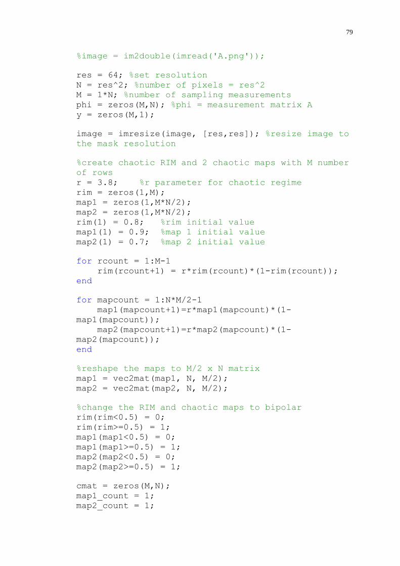
79

%image = im2double(imread('A.png'));

res = 64; %set resolution

N = res^2; %number of pixels = res^2

M = 1*N; %number of sampling measurements

phi = zeros(M,N); %phi = measurement matrix A

y = zeros(M,1);

image = imresize(image, [res,res]); %resize image to

the mask resolution

%create chaotic RIM and 2 chaotic maps with M number

of rows

r = 3.8; %r parameter for chaotic regime

rim = zeros(1,M);

map1 = zeros(1,M*N/2);

map2 = zeros(1,M*N/2);

rim(1) = 0.8; %rim initial value

map1(1) = 0.9; %map 1 initial value

map2(1) = 0.7; %map 2 initial value

for rcount = 1:M-1

rim(rcount+1) = r*rim(rcount)*(1-rim(rcount));

end

for mapcount = 1:N*M/2-1

map1(mapcount+1)=r*map1(mapcount)*(1-

map1(mapcount));

map2(mapcount+1)=r*map2(mapcount)*(1-

map2(mapcount));

end

%reshape the maps to M/2 x N matrix

map1 = vec2mat(map1, N, M/2);

map2 = vec2mat(map2, N, M/2);

%change the RIM and chaotic maps to bipolar

rim(rim<0.5) = 0;

rim(rim>=0.5) = 1;

map1(map1<0.5) = 0;

map1(map1>=0.5) = 1;

map2(map2<0.5) = 0;

map2(map2>=0.5) = 1;

cmat = zeros(M,N);

map1_count = 1;

map2_count = 1;

80

currentmap = 1;

for count = 1:M

if map1_count > M/2

cmat(count:M,:)=map2(map2_count:M/2,:);

break;

elseif map2_count > M/2

cmat(count:M,:)=map1(map1_count:M/2,:);

break;

end

if rim(count)==1

if currentmap == 1

cmat(count,:) = map2(map2_count,:);

currentmap = 2;

map2_count = map2_count+1;

elseif currentmap == 2;

cmat(count,:) = map1(map1_count,:);

currentmap = 1;

map1_count = map1_count+1;

end

else

if currentmap == 1

cmat(count,:) = map1(map1_count,:);

map1_count = map1_count+1;

elseif currentmap == 2;

cmat(count,:) = map2(map2_count,:);

map2_count = map2_count+1;

end

end

end

%find y

startmask = tic; %start stopwatch

for ip = 1:M

%arrange chaotic mask pattern into res x res

matrix

H(:,:,ip) = vec2mat(cmat(ip,:),res);

mask = H(:,:,ip);

%reshape each chaotic mask to the size of the

image

csamp = imresize(mask,size(image),'nearest');

%project pattern sequence to image

temp = image;

temp(csamp==0) = 0;

81

%record average intensity

y(ip) = sum(sum(temp))./numel(temp);

end

endmask = toc(startmask); %stop stopwatch and record

the reading time

%%

%%%%%%%%%%%%%%%%%%%%%%%%%%%%%%%%%%%%%%%%%%%%%%%%%%%%

%%%%%%

A = transpose(y);

yy=A;

rng(2);

A1=rand(1,M);

A11=exp(j*2*pi*A1);%mask1

A111=A.*A11;

B=fft2(A111);

rng(4);

B1=rand(1,M);

B11=exp(j*2*pi*B1);%mask2

B111=B.*B11;

C=ifft2(B111);

C1=abs(C);

imC1=vec2mat(C1,46,46);

figure;imshow(imC1);title('The Encrypted image');

%decryption

% [s1 s2] = size(C);

% sigma = 10;

% Enoise = zeros(s1,s2);

% Enoise(:,:) = normrnd(0,sigma,s1,s2)+ i *

normrnd(0,sigma,s1,s2);

% C = C + Enoise;

D=fft2(C);

D1=D.*exp(-j*2*pi*B1);

D11=ifft2(D1);

D111=D11.*exp(-j*2*pi*A1);

F=abs(D11);

F = transpose(F);

%figure,imshow(F);title('The decrypted image');

%%%%%%%%%%%%%%%%%%%%%%%%%%%%%%%%%%%%%%%%%%%%%%%%%%%%

%%%%%%%%%%%%

%%

%solve and reconstruct image

% Find x, image represention --> estIm

% y = Ax

% x = A-1*y = A\y --> inverse A

82

% Note: x = img0/estIm (Nx1), A = phi (MxN), y =

aver (Mx1)

startrecon = tic; %start stopwatch

%get phi using correct seed

%create chaotic RIM and 2 chaotic maps with M number

of rows

r = 3.8; %r parameter for chaotic regime

rim = zeros(1,M);

map1 = zeros(1,M*N/2);

map2 = zeros(1,M*N/2);

rim(1) = 0.8; %rim initial value

map1(1) = 0.9; %map 1 initial value

map2(1) = 0.7; %map 2 initial value

for rcount = 1:M-1

rim(rcount+1) = r*rim(rcount)*(1-rim(rcount));

end

for mapcount = 1:N*M/2-1

map1(mapcount+1)=r*map1(mapcount)*(1-

map1(mapcount));

map2(mapcount+1)=r*map2(mapcount)*(1-

map2(mapcount));

end

%reshape the maps to M/2 x N matrix

map1 = vec2mat(map1, N, M/2);

map2 = vec2mat(map2, N, M/2);

%change the RIM and chaotic maps to bipolar

rim(rim<0.5) = 0;

rim(rim>=0.5) = 1;

map1(map1<0.5) = 0;

map1(map1>=0.5) = 1;

map2(map2<0.5) = 0;

map2(map2>=0.5) = 1;

cmat = zeros(M,N);

map1_count = 1;

map2_count = 1;

currentmap = 1;

for count = 1:M

if map1_count > M/2

cmat(count:M,:)=map2(map2_count:M/2,:);

break;

elseif map2_count > M/2

83

cmat(count:M,:)=map1(map1_count:M/2,:);

break;

end

if rim(count)==1

if currentmap == 1

cmat(count,:) = map2(map2_count,:);

currentmap = 2;

map2_count = map2_count+1;

elseif currentmap == 2;

cmat(count,:) = map1(map1_count,:);

currentmap = 1;

map1_count = map1_count+1;

end

else

if currentmap == 1

cmat(count,:) = map1(map1_count,:);

map1_count = map1_count+1;

elseif currentmap == 2;

cmat(count,:) = map2(map2_count,:);

map2_count = map2_count+1;

end

end

end

for ip = 1:M

H(:,:,ip) = vec2mat(cmat(ip,:),res);

mask = H(:,:,ip);

phi(ip,:) = cmat(ip,:);

end

invphi = pinv(phi);%pinv(A) returns the Moore-

Penrose Pseudoinverse of matrix A.

im0 = invphi*F;%initial solution

estIm = l1dantzig_pd(im0, phi, [], F, 0.01, 1e-4,2);

% Reconstruct image

reconIm = vec2mat(estIm,res);

reconIm = (reconIm-

min(min(reconIm)))/(max(max(reconIm))-

min(min(reconIm)));%normalize image

endrecon = toc(startrecon); %end stopwatch and

record reconstruction time

84

%%

%calculate RMSE

A = zeros(res,res);

scaled_image = imresize(image,size(A));

o = vec2mat(scaled_image,1);

o_un = vec2mat(reconIm,1);

for i = 1:N

diff = (o_un(i,1) - o(i,1));

diff_sq(i,:) = diff^2;

end

diff_sq_sum = sum(diff_sq,1);

RMSE = sqrt(diff_sq_sum/N);

%calculate PSNR

peaksnr = psnr(reconIm, scaled_image);

%calculate SSIM

ssimval = ssim(reconIm, scaled_image);

%calculate CC

ccval = corr2(scaled_image, reconIm);

%calculate M/N

MNratio = M/N;

%show the rescaled image

figure;

subplot(1,2,1); imshow(scaled_image);

title('Rescaled image');

%show the reconstructed image

subplot(1,2,2); imshow(reconIm);

title(['Reconstructed image']);

%%

%Security analysis

%histogram analysis

figure; subplot(1,2,1);

imhist(C1); title('histogram of final ciphertext');

[ycounts, ybinLocations] = imhist(C1);

subplot(1,2,2);

imhist(scaled_image); title('histogram of image');

[imcounts, imbinLocations] = imhist(scaled_image);%

title('histogram of image');

%image entropy

%y_entropy = entropy(y);

85

%histogram variance

imdata=reshape(transpose(scaled_image),1,[]);

v = var(ycounts);

vim = var(imcounts);

%differential attack analysis: NPCR & UACI

img_chg = image;

img_chg(1,1) = 1;

y_chg = zeros(M,1);

for ip = 1:M

mask = H(:,:,ip);

csamp = mask;

%project pattern sequence to image

temp = img_chg;

temp(csamp==0) = 0;

%record average intensity

y_chg(ip) = sum(sum(temp))./numel(temp);

end

A = transpose(y_chg);

yy=A;

rng(2);

A1=rand(1,M);

A11=exp(j*2*pi*A1);%mask1

A111=A.*A11;

B=fft2(A111);

rng(4);

B1=rand(1,M);

B11=exp(j*2*pi*B1);%mask2

B111=B.*B11;

C=ifft2(B111);

C1_chg=abs(C); %changed final ciphertext

C1 = round(255.*C1);

C1_chg = round(255.*C1_chg);

D = 0;

diffsum = 0;

for i=1:M

if(C1(i)~=C1_chg(i))

D = D + 1;

end

diffsum = diffsum + abs(C1(i) - C1_chg(i))/255;

end

NPCR = (D/M)*100;

UACI = 100*diffsum/M;

86

%%

%tabulate results

T = table(MNratio, RMSE, peaksnr, ssimval, ccval,

endmask, endrecon);

disp(T);

new_chaotic_rsa.m

clear all

addpath(genpath('l1magic'))

% Simulation using test image

image = rgb2gray(im2double(imread('192.png')));

%image = im2double(imread('A.png'));

res = 64; %set resolution

N = res^2; %number of pixels = res^2

M = 1*N; %number of sampling measurements

phi = zeros(M,N); %phi = measurement matrix A

y = zeros(M,1);

image = imresize(image, [res,res]); %resize image to

the mask resolution

%create chaotic RIM and 2 chaotic maps with M number

of rows

r = 3.8; %r parameter for chaotic regime

rim = zeros(1,M);

map1 = zeros(1,M*N/2);

map2 = zeros(1,M*N/2);

rim(1) = 0.8; %rim initial value

map1(1) = 0.9; %map 1 initial value

map2(1) = 0.7; %map 2 initial value

for rcount = 1:M-1

rim(rcount+1) = r*rim(rcount)*(1-rim(rcount));

end

for mapcount = 1:N*M/2-1

map1(mapcount+1)=r*map1(mapcount)*(1-

map1(mapcount));

map2(mapcount+1)=r*map2(mapcount)*(1-

map2(mapcount));

end

%reshape the maps to M/2 x N matrix

87

map1 = vec2mat(map1, N, M/2);

map2 = vec2mat(map2, N, M/2);

%change the RIM and chaotic maps to bipolar

rim(rim<0.5) = 0;

rim(rim>=0.5) = 1;

map1(map1<0.5) = 0;

map1(map1>=0.5) = 1;

map2(map2<0.5) = 0;

map2(map2>=0.5) = 1;

cmat = zeros(M,N);

map1_count = 1;

map2_count = 1;

currentmap = 1;

for count = 1:M

if map1_count > M/2

cmat(count:M,:)=map2(map2_count:M/2,:);

break;

elseif map2_count > M/2

cmat(count:M,:)=map1(map1_count:M/2,:);

break;

end

if rim(count)==1

if currentmap == 1

cmat(count,:) = map2(map2_count,:);

currentmap = 2;

map2_count = map2_count+1;

elseif currentmap == 2;

cmat(count,:) = map1(map1_count,:);

currentmap = 1;

map1_count = map1_count+1;

end

else

if currentmap == 1

cmat(count,:) = map1(map1_count,:);

map1_count = map1_count+1;

elseif currentmap == 2;

cmat(count,:) = map2(map2_count,:);

map2_count = map2_count+1;

end

end

end

%find y

startmask = tic; %start stopwatch

88

for ip = 1:M

%arrange chaotic mask pattern into res x res

matrix

H(:,:,ip) = vec2mat(cmat(ip,:),res);

mask = H(:,:,ip);

%reshape each chaotic mask to the size of the

image

csamp = imresize(mask,size(image),'nearest');

%project pattern sequence to image

temp = image;

temp(csamp==0) = 0;

%record average intensity

y(ip) = sum(sum(temp))./numel(temp);

end

endmask = toc(startmask); %stop stopwatch and record

the reading time

%solve and reconstruct image

% Find x, image represention --> estIm

% y = Ax

% x = A-1*y = A\y --> inverse A

% Note: x = img0/estIm (Nx1), A = phi (MxN), y =

aver (Mx1)

startrecon = tic; %start stopwatch

%get phi using correct seed

%create chaotic RIM and 2 chaotic maps with M number

of rows

r = 3.8; %r parameter for chaotic regime

rim = zeros(1,M);

map1 = zeros(1,M*N/2);

map2 = zeros(1,M*N/2);

rim(1) = 0.8; %rim initial value

map1(1) = 0.9; %map 1 initial value

map2(1) = 0.7; %map 2 initial value

for rcount = 1:M-1

rim(rcount+1) = r*rim(rcount)*(1-rim(rcount));

end

for mapcount = 1:N*M/2-1

map1(mapcount+1)=r*map1(mapcount)*(1-

map1(mapcount));

89

map2(mapcount+1)=r*map2(mapcount)*(1-

map2(mapcount));

end

%reshape the maps to M/2 x N matrix

map1 = vec2mat(map1, N, M/2);

map2 = vec2mat(map2, N, M/2);

%change the RIM and chaotic maps to bipolar

rim(rim<0.5) = 0;

rim(rim>=0.5) = 1;

map1(map1<0.5) = 0;

map1(map1>=0.5) = 1;

map2(map2<0.5) = 0;

map2(map2>=0.5) = 1;

cmat = zeros(M,N);

map1_count = 1;

map2_count = 1;

currentmap = 1;

for count = 1:M

if map1_count > M/2

cmat(count:M,:)=map2(map2_count:M/2,:);

break;

elseif map2_count > M/2

cmat(count:M,:)=map1(map1_count:M/2,:);

break;

end

if rim(count)==1

if currentmap == 1

cmat(count,:) = map2(map2_count,:);

currentmap = 2;

map2_count = map2_count+1;

elseif currentmap == 2;

cmat(count,:) = map1(map1_count,:);

currentmap = 1;

map1_count = map1_count+1;

end

else

if currentmap == 1

cmat(count,:) = map1(map1_count,:);

map1_count = map1_count+1;

elseif currentmap == 2;

cmat(count,:) = map2(map2_count,:);

map2_count = map2_count+1;

end

90

end

end

for ip = 1:M

H(:,:,ip) = vec2mat(cmat(ip,:),res);

mask = H(:,:,ip);

phi(ip,:) = cmat(ip,:);

end

%% RSA

%change y to 0-255

ky = 255.*y;

ky = ky - floor(ky);

y255 = floor(255.*y);

%calculate the value of p & q

rng(3);

temp=randi([3 30],1,M);

p=nthprime(temp);

q = zeros(1,M);

rng(5);

for count = 1:M

q(count)=nthprime(randi([3 30]));

while(p(count)*q(count)<256 ||

p(count)==q(count))

q(count)=nthprime(randi([3 30]));

end

end

n=p.*q;

%calculate the value of phi

Phi = (p-1).*(q-1);

%calculate the value of e

e=ones(1,M);

for count = 1:M

x=2;

while x > 1

e(count)=e(count)+1;

x=gcd(Phi(count),e(count));

end

end

%calculate the value of d

d = zeros(1,M);

for count = 1:M

rem=0;

while(rem~=1);

d(count)=d(count)+1;

rem=mod(d(count)*e(count),Phi(count));

end

end

91

% % %Encryption, %c=mod(m.^e,n);

cr=zeros(1,M);

for count = 1:M

eb=dec2bin_rsa(e(count));

k = 65535;

c = y255(count);

cf = 1;

cf=mod(c*cf,n(count));

for i=k-1:-1:1

c = mod(c*c,n(count));

j=k-i+1;

if eb(j)==1

cf=mod(c*cf,n(count));

end

end

cr(count)=cf;

end

%Convert to proper intensity level

r = mod(cr,256);

K = (cr-r)./256;

% % %Decryption, %mr=mod(c.^d,n);

cr1 = 256.*K + r;

mr = zeros(1,M);

for count = 1:M

db=dec2bin_rsa(d(count));

k = 65535;

c = cr(count);

cf = 1;

cf=mod(c*cf,n(count));

for i=k-1:-1:1

c = mod(c.*c,n(count));

j=k-i+1;

if db(j)==1

cf=mod(c*cf,n(count));

end

end

mr(count)=cf;

end

y_rec = (transpose(mr)+ky)./255;

%%

invphi = pinv(phi);%pinv(A) returns the Moore-

Penrose Pseudoinverse of matrix A.

im0 = invphi*y_rec;%initial solution

92

estIm = l1dantzig_pd(im0, phi, [], y_rec, 0.01, 1e-

4,2);

% Reconstruct image

reconIm = vec2mat(estIm,res);

reconIm = (reconIm-

min(min(reconIm)))/(max(max(reconIm))-

min(min(reconIm)));%normalize image

endrecon = toc(startrecon); %end stopwatch and

record reconstruction time

%calculate RMSE

A = zeros(res,res);

scaled_image = imresize(image,size(A));

o = vec2mat(scaled_image,1);

o_un = vec2mat(reconIm,1);

for i = 1:N

diff = (o_un(i,1) - o(i,1));

diff_sq(i,:) = diff^2;

end

diff_sq_sum = sum(diff_sq,1);

RMSE = sqrt(diff_sq_sum/N);

%calculate PSNR

peaksnr = psnr(reconIm, scaled_image);

%calculate SSIM

ssimval = ssim(reconIm, scaled_image);

%calculate CC

ccval = corr2(scaled_image, reconIm);

%calculate M/N

MNratio = M/N;

%show the rescaled image

figure;

subplot(1,2,1); imshow(scaled_image);

title('Rescaled image');

%show the reconstructed image

subplot(1,2,2); imshow(reconIm);

title(['Reconstructed image']);

%%

%Security analysis

93

%histogram analysis

figure; subplot(1,2,1);

imhist(r/255); title('histogram of final

ciphertext');

[ycounts, ybinLocations] = imhist(r/255);

subplot(1,2,2);

imhist(scaled_image); title('histogram of image');

[imcounts, imbinLocations] = imhist(scaled_image);%

title('histogram of image');

%image entropy

%y_entropy = entropy(y);

%histogram variance

imdata=reshape(transpose(scaled_image),1,[]);

v = var(ycounts);

vim = var(imcounts);

%differential attack analysis: NPCR & UACI

img_chg = image;

img_chg(1,1) = 1;

y_chg = zeros(M,1);

for ip = 1:M

mask = H(:,:,ip);

csamp = mask;

%project pattern sequence to image

temp = img_chg;

temp(csamp==0) = 0;

%record average intensity

y_chg(ip) = sum(sum(temp))./numel(temp);

end

% % %Encryption, %c=mod(m.^e,n);

cr_chg=zeros(1,M);

for count = 1:M

eb=dec2bin_rsa(e(count));

k = 65535;

c = y_chg(count);

cf = 1;

cf=mod(c*cf,n(count));

for i=k-1:-1:1

c = mod(c*c,n(count));

j=k-i+1;

if eb(j)==1

cf=mod(c*cf,n(count));

94

end

end

cr_chg(count)=cf;

end

%Convert to proper intensity level

r_chg = mod(cr_chg,256);

D = 0;

diffsum = 0;

for i=1:M

if(r(i)~=r_chg(i))

D = D + 1;

end

diffsum = diffsum + abs(r(i) - r_chg(i))/255;

end

NPCR = (D/M)*100;

UACI = 100*diffsum/M;

%%

%tabulate results

T = table(MNratio, RMSE, peaksnr, ssimval, ccval,

endmask, endrecon);

disp(T);

dec2bin_rsa.m

function a = dec2bin_rsa(d)

i=1;

a=zeros(1,65535);

while d >= 2

r=rem(d,2);

if r==1

a(i)=1;

else

a(i)=0;

end

i=i+1;

d=floor(d/2);

end

if d == 2

a(i) = 0;

else

a(i) = 1;

end

x=[a(16) a(15) a(14) a(13) a(12) a(11) a(10) a(9)

a(8) a(7) a(6) a(5) a(4) a(3) a(2) a(1)];