www.iap.uni-jena.de

Optical Design with Zemaxfor PhD - Basics

Lecture 5: Aberrations II

2014-05-22

Herbert Gross

Summer term 2014

2

Preliminary Schedule

No Date Subject Detailed content

1 16.04. IntroductionZemax interface, menus, file handling, system description, editors, preferences, updates, system reports, coordinate systems, aperture, field, wavelength, layouts, diameters, stop and pupil, solves

2 24.04. Basic Zemax handling Raytrace, ray fans, paraxial optics, surface types, quick focus, catalogs, vignetting, footprints, system insertion, scaling, component reversal

3 08.05. Properties of optical systems aspheres, gradient media, gratings and diffractive surfaces, special types of surfaces, telecentricity, ray aiming, afocal systems

4 15.05. Aberrations I representations, spot, Seidel, transverse aberration curves, Zernike wave aberrations

5 22.05. Aberrations II PSF, MTF, ESF

6 05.06. Optimization I algorithms, merit function, variables, pick up’s

7 12.06. Optimization II methodology, correction process, special requirements, examples

8 19.06. Advanced handling slider, universal plot, I/O of data, material index fit, multi configuration, macro language

9 25.06. Imaging Fourier imaging, geometrical images

10 03.07. Correction I simple and medium examples

11 10.07. Correction II advanced examples

12 xx.07. Illumination simple illumination calculations, non-sequential option

13 xx.07. Physical optical modelling I Gaussian beams, POP propagation

14 xx.07. Physical optical modelling II polarization raytrace, polarization transmission, polarization aberrations, coatings, representations, transmission and phase effects

15 xx.07. Tolerancing Sensitivities, Tolerancing, Adjustment

1. Point spread function

2. Edge and line spread function

3. Optical transfer function

3

Contents

Diffraction at the System Aperture

Self luminous points: emission of spherical waves Optical system: only a limited solid angle is propagated, the truncaton of the spherical wave

results in a finite angle light cone In the image space: uncomplete constructive interference of partial waves, the image point

is spreaded The optical systems works as a low pass filter

objectpoint

sphericalwave

truncatedspherical

wave

imageplane

x = 1.22 / NA

pointspread

function

object plane

Fraunhofer Point Spread Function

Rayleigh-Sommerfeld diffraction integral, Mathematical formulation of the Huygens-principle

Fraunhofer approximation in the far fieldfor large Fresnel number

Optical systems: numerical aperture NA in image spacePupil amplitude/transmission/illumination T(xp,yp)Wave aberration W(xp,yp)complex pupil function A(xp,yp)Transition from exit pupil to image plane

Point spread function (PSF): Fourier transform of the complex pupil function

12

z

rN p

F

),(2),(),( pp yxWipppp eyxTyxA

pp

yyxxR

iyxiW

ppAP

dydxeeyxTyxEpp

APpp''2

,2,)','(

''cos'

)'()('

dydxrr

erEirE d

rrki

I

PSF by Huygens Principle

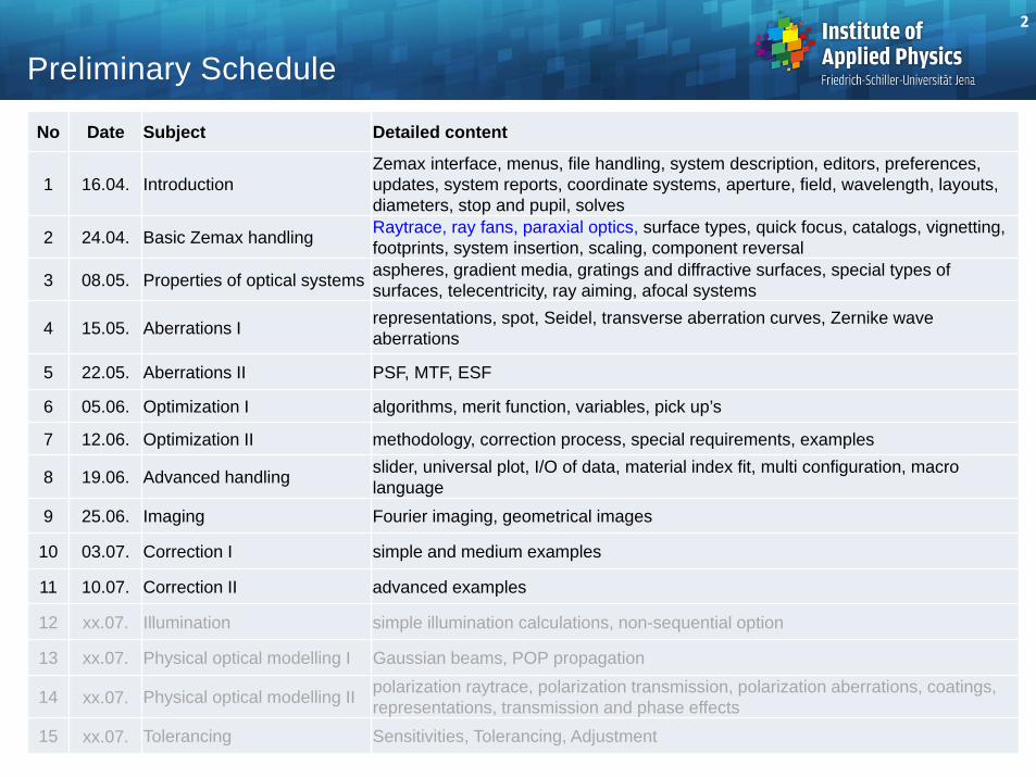
Huygens wavelets correspond to vectorial field components The phase is represented by the direction The amplitude is represented by the length Zeros in the diffraction pattern: destructive interference Aberrations from spherical wave: reduced conctructive superposition

0

212,0 Iv

vJvI

0

2

4/4/sin0, I

uuuI

-25 -20 -15 -10 -5 0 5 10 15 20 250,0

0,2

0,4

0,6

0,8

1,0

vertical lateral

inte

nsity

u / v

Circular homogeneous illuminatedAperture: intensity distribution transversal: Airy

scale:

axial: sincscale

Resolution transversal betterthan axial: x < z

Ref: M. Kempe

Scaled coordinates according to Wolf : axial : u = 2 z n / NA2

transversal : v = 2 x / NA

Perfect Point Spread Function

NADAiry

22.1

2NAnRE

log I(r)

r0 5 10 15 20 25 3010

10

10

10

10

10

10

-6

-5

-4

-3

-2

-1

0Airy distribution:

Gray scale picture Zeros non-equidistant Logarithmic scale Encircled energy

Perfect Lateral Point Spread Function: Airy

DAiry

r / rAiry

Ecirc(r)

0

1

2 3 4 5

1.831 2.655 3.477

0

0.1

0.2

0.3

0.4

0.5

0.6

0.7

0.8

0.9

1

2. ring 2.79%

3. ring 1.48%

1. ring 7.26%

peak 83.8%

Axial distribution of intensityCorresponds to defocus

Normalized axial coordinate

Scale for depth of focus :Rayleigh length

Zero crossing points:equidistant and symmetric,Distance zeros around image plane 4RE

22

0 4/4/sinsin)(

uuI

zzIzI o

42

2 uzNAz

22

''sin' NA

nun

RE

Perfect Axial Point Spread Function

Defocussed Perfect Psf

Perfect point spread function with defocus Representation with constant energy: extreme large dynamic changes

z = -2RE z = +2REz = -1RE z = +1RE

normalizedintensity

constantenergy

focus

Imax = 5.1% Imax = 42%Imax = 9.8%

Comparison Geometrical Spot – Wave-Optical Psf

aberrations

spotdiameter

DAiry

exactwave-optic

geometric-opticapproximated

diffraction limited,failure of the

geometrical model

Fourier transformill conditioned

Large aberrations:Waveoptical calculation shows bad conditioning

Wave aberrations small: diffraction limited, geometrical spot too small and wrong

Approximation for the intermediate range:

22GeoAirySpot DDD

0,0

0,0)(

)(

idealPSF

realPSF

S IID

2

2),(2

),(

),(

dydxyxA

dydxeyxAD

yxWi

S

Important citerion for diffraction limited systems:Strehl ratio (Strehl definition)Ratio of real peak intensity (with aberrations) referenced on ideal peak intensity

DS takes values between 0...1DS = 1 is perfect

Critical in use: the completeinformation is reduced to only one number

The criterion is useful for 'good'systems with values Ds > 0.5

Strehl Ratio

r

1

peak reducedStrehl ratio

distributionbroadened

ideal , withoutaberrations

real withaberrations

I(x )

12

Psf with Aberrations

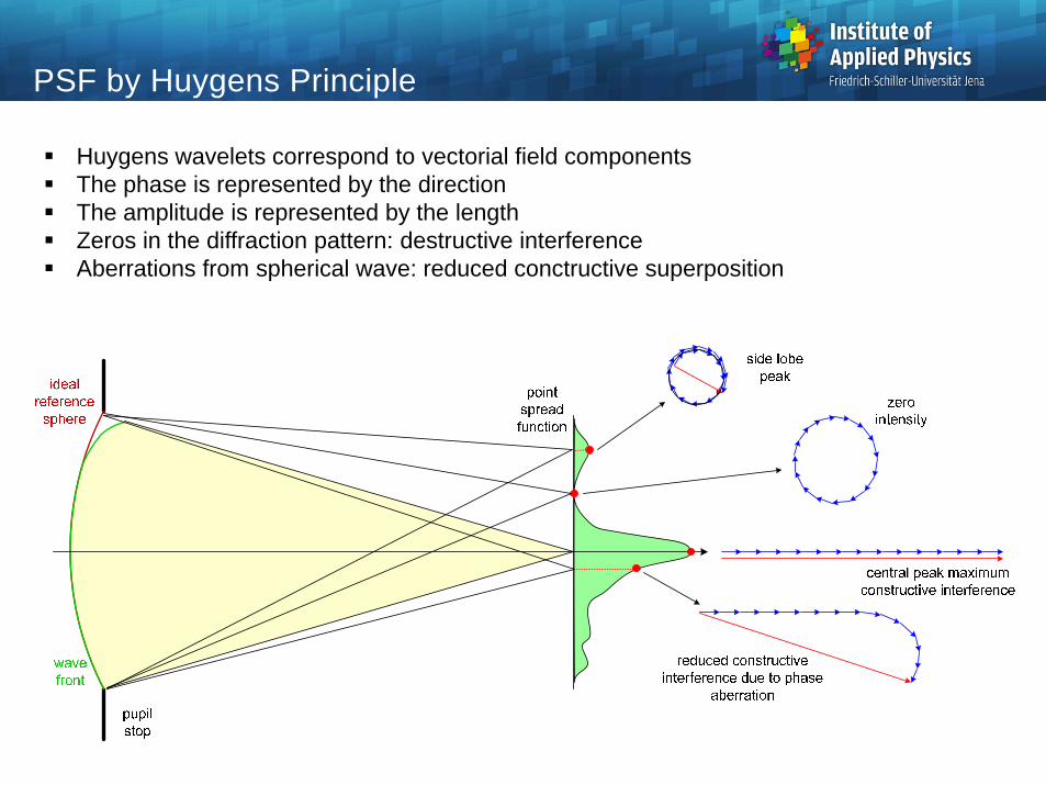
Psf for some low oder Zernike coefficients The coefficients are changed between cj = 0...0.7 The peak intensities are renormalized

spherical

defocus

coma

astigmatism

trefoil

spherical 5. order

astigmatism 5. order

coma 5. order

c = 0.0c = 0.1

c = 0.2c = 0.3

c = 0.4c = 0.5

c = 0.7

13

Point Spread Function with Apodization

w

I(w)

1

0.8

0.6

0.4

0.2

00 1 2 3-2 -1

AiryBesselGauss

FWHM

Apodisation of the pupil:1. Homogeneous2. Gaussian3. Bessel

Psf in focus:different convergence to zero forlarger radii

Encircled energy:same behavior

Complicated:Definition of compactness of thecentral peak:

1. FWHM: Airy more compact as GaussBessel more compact as Airy

2. Energy 95%: Gauss more compact as AiryBessel extremly worse

Only far field model (Fraunhofer)

Two different algorithms available:1. FFT-based

- fast- equidistant exit pupil sampling assumed- high resolution PSF needs many points

2. elementary integration (Huygens)- slow (N4)- independence of pupil and image sampling- valid also for calculation of pupil distortion- gives correct Strehl number

Different options for representation possible

15

PSF in Zemax

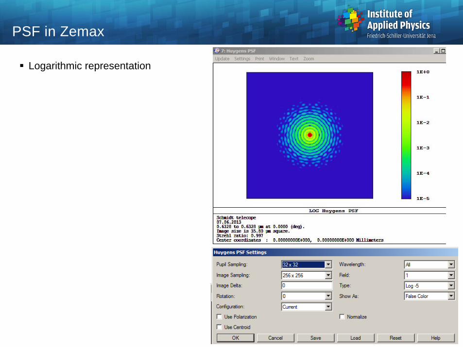
Logarithmic representation

16

PSF in Zemax

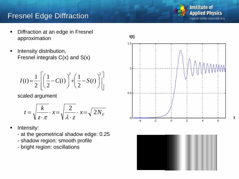
Diffraction at an edge in Fresnelapproximation

Intensity distribution,Fresnel integrals C(x) and S(x)

scaled argument

Intensity:- at the geometrical shadow edge: 0.25- shadow region: smooth profile- bright region: oscillations

22

)(21)(

21

21)( tStCtI

FNxz

xzkt 22

t

-4 -2 0 2 4 60

0.5

1

1.5

I(t)

Fresnel Edge Diffraction

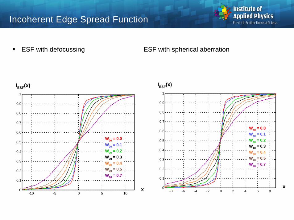
ESF with defocussing ESF with spherical aberration

x

IESF(x)

-10 -5 0 5 100

0.1

0.2

0.3

0.4

0.5

0.6

0.7

0.8

0.9

1

W20 = 0.0W20 = 0.1W20 = 0.2W20 = 0.3W20 = 0.4W20 = 0.5W20 = 0.7

x

IESF(x)

-8 -6 -4 -2 0 2 4 6 80

0.1

0.2

0.3

0.4

0.5

0.6

0.7

0.8

0.9

1

W40 = 0.0W40 = 0.1W40 = 0.2W40 = 0.3W40 = 0.4W40 = 0.5W40 = 0.7

Incoherent Edge Spread Function

Line image: integral over point sptread functionLSF: line spread function

Realization: narrow slitconvolution of slit width

But with deconvolution, the PSF can be reconstructed

dyyxIxI PSFLSF ),()(

Integration

intensity

x

Line spread function

PSF

dyyxIxI PSFLSF ),()(

Linienbild

Line image:Fourier transform of pupil in one dimension

Line spreadfunction with aberrationsHere: defocussing

pppp

pp

xxRi

pp

iLSFdydxyxP

dydxeyxP

xI

pi

2

22

,

,

)(

x

ILSF(x)

-10 -5 0 5 100

0.1

0.2

0.3

0.4

0.5

0.6

0.7

0.8

0.9

1

W20 = 0.0W20 = 0.1W20 = 0.2W20 = 0.3W20 = 0.4W20 = 0.5W20 = 0.7

Line Spread Function

Sampling of the Diffraction Integral

x-6 -4 -2 0 2 4

0

10

20

30

40

50quadratic

phase

wrappedphase

2

smallest samplingintervall

phase

Oscillating exponent :Fourier transform reduces on 2-period Most critical sampling usually

at boundary defines numberof sampling points Steep phase gradients define the

sampling High order aberrations are a

problem

Propagation by Plane / Spherical Waves

Expansion field in simple-to-propagate waves

1. Spherical waves 2. Plane wavesHuygens principle spectral representation

rdrErr

erErrik

2'

)('

)'(

)(ˆˆ)'( 1 rEFeFrE xy

zikxy

z

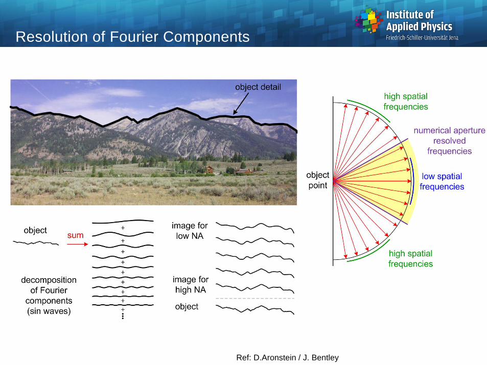
Resolution of Fourier Components

Ref: D.Aronstein / J. Bentley

pppp

ppvyvxi

pp

yxOTF

dydxyxg

dydxeyxgvvH

ypxp

2

22

),(

),(),(

),(ˆ),( yxIFvvH PSFyxOTF

pppp

ppy

px

py

px

p

yxOTF

dydxyxP

dydxvf

yvfxPvf

yvfxPvvH

2

*

),(

)2

,2

()2

,2

(),(

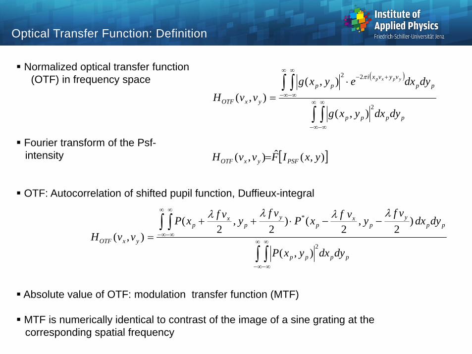
Optical Transfer Function: Definition

Normalized optical transfer function(OTF) in frequency space

Fourier transform of the Psf-intensity

OTF: Autocorrelation of shifted pupil function, Duffieux-integral

Absolute value of OTF: modulation transfer function (MTF)

MTF is numerically identical to contrast of the image of a sine grating at thecorresponding spatial frequency

I Imax V 0.010 0.990 0.980 0.020 0.980 0.961 0.050 0.950 0.905 0.100 0.900 0.818 0.111 0.889 0.800 0.150 0.850 0.739 0.200 0.800 0.667 0.300 0.700 0.538

Contrast / Visibility

The MTF-value corresponds to the intensity contrast of an imaged sin grating Visibility

The maximum value of the intensityis not identical to the contrast valuesince the minimal value is finite too

Concrete values:

minmax

minmax

IIIIV

I(x)

-2 -1.5 -1 -0.5 0 1 1.5 2

0

0.1

0.2

0.3

0.4

0.5

0.6

0.7

0.8

0.9

1

x

Imax

Imin

object

image

peakdecreased

slopedecreased

minimaincreased

Number of Supported Orders

A structure of the object is resolved, if the first diffraction order is propagatedthrough the optical imaging system

The fidelity of the image increases with the number of propagated diffracted orders

Optical Transfer Function of a Perfect System

Aberration free circular pupil:Reference frequency

Maximum cut-off frequency:

Analytical representation

Separation of the complex OTF function into:- absolute value: modulation transfer MTF- phase value: phase transfer function PTF

'sinu

favo

'sin222 0max

unf

navv

2

000 21

22arccos2)(

vv

vv

vvvHMTF

),(),(),( yxPTF vvHiyxMTFyxOTF evvHvvH

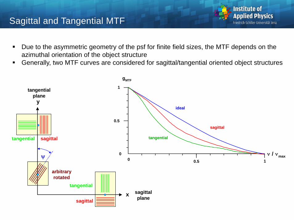
Due to the asymmetric geometry of the psf for finite field sizes, the MTF depends on theazimuthal orientation of the object structure

Generally, two MTF curves are considered for sagittal/tangential oriented object structures

Sagittal and Tangential MTF

y

tangentialplane

tangential sagittal

arbitraryrotated

x sagittalplane

tangential

sagittal

gMTF

tangential

ideal

sagittal

1

0

0.5

0 0.5 1 / max

x

y

x

y

L

L

x

y

o

o

x'

y'

p

p

light source

condenserconjugate to object pupil

object

objectivepupil

directlight

at object diffracted light in 1st order

Interpretation of the Duffieux Iintegral

Interpretation of the Duffieux integral:overlap area of 0th and 1st diffraction order,interference between the two orders

The area of the overlap corresponds to theinformation transfer of the structural details

Frequency limit of resolution:areas completely separated

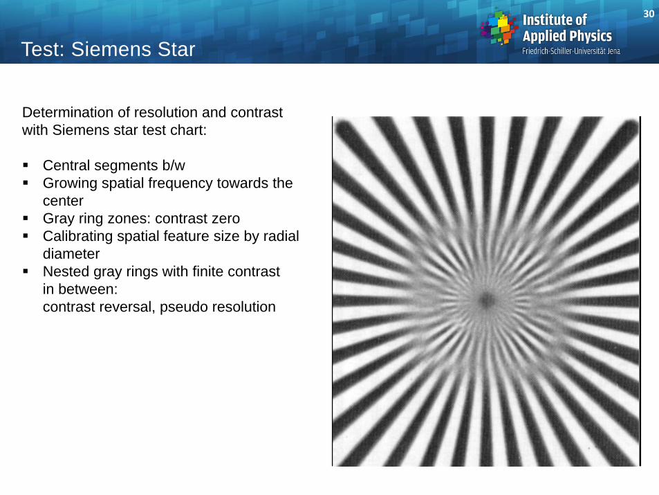
Test: Siemens Star

Determination of resolution and contrast with Siemens star test chart:

Central segments b/w Growing spatial frequency towards the

center Gray ring zones: contrast zero Calibrating spatial feature size by radial

diameter Nested gray rings with finite contrast

in between:contrast reversal, pseudo resolution

30

Contrast and Resolution

High frequent structures :contrast reduced

Low frequent structures:resolution reduced

contrast

resolution

brillant

sharpblurred

milky

31

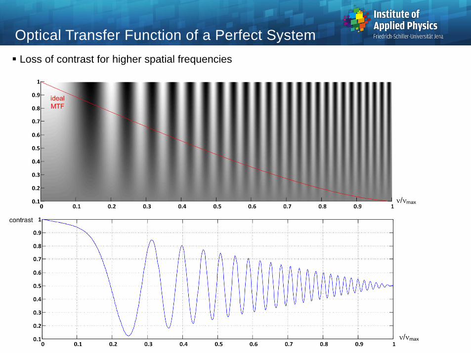
Optical Transfer Function of a Perfect System Loss of contrast for higher spatial frequencies

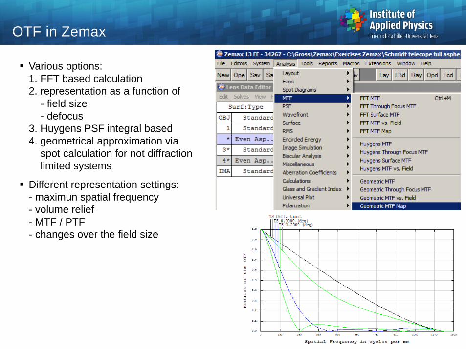
Various options:1. FFT based calculation2. representation as a function of

- field size- defocus

3. Huygens PSF integral based4. geometrical approximation via

spot calculation for not diffractionlimited systems

Different representation settings:- maximun spatial frequency- volume relief- MTF / PTF- changes over the field size

33

OTF in Zemax

Various MTF representations

34

OTF in Zemax