Optical Design with Zemax - Institute of Applied Physics · 2012-11-21 · 3. ABg scattering...
74
www.iap.uni-jena.de Optical Design with Zemax Lecture 10: Physical Optical Modelling II 2012-11-22 Herbert Gross Summer term 2012
Transcript of Optical Design with Zemax - Institute of Applied Physics · 2012-11-21 · 3. ABg scattering...
www.iap.uni-jena.de
Optical Design with Zemax
Lecture 10: Physical Optical Modelling II
2012-11-22
Herbert Gross
Summer term 2012

2 10 Physical Optical Modelling II
Preliminary time schedule

1. Coatings
2. Coating transmission and phase effects
3. Ghost imaging
4. Straylight
5. Scattering in Zemax
6. Fresnel equations
7. Overview
8. Design and calculation of thin films
9. Simple layers
10.Representations
11.Applications and examples
12.Coatings in Zemax
3 10 Physical Optical Modelling II
Contents

10 Physical Optical Modelling II
Ghost Images
Ghost image in photographic lenses:
Reflex film / surface
Ref: K. Uhlendorf, D. Gängler

Different reasons
Various distributions
10 Physical Optical Modelling II
Straylight and Ghost Images
a b

10 Physical Optical Modelling II
Scattering of Light
Scattering of light in diffuse media like frog
Ref: W. Osten
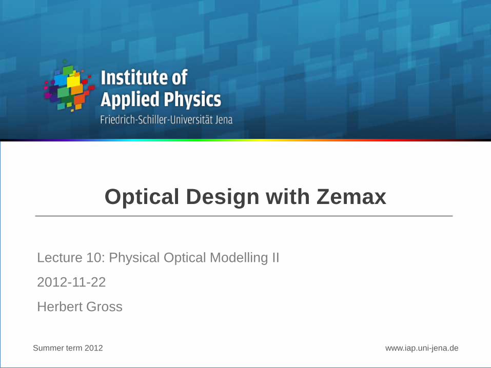
Calculation of reflected light
Colour effects due to coatings
10 Physical Optical Modelling II
Straylight and Ghost Images
Ref.: M. Peschka
sequence 5 - 3
3
5
sequence 6 - 4
4
6
6 - 4
5 - 3
9 - 3
7 - 2
14 - 1115 - 11
20 - 18sequence 13 - 4 sequence 13 - 5
sequence 7 - 2
sequence 20 - 18
sequence 6 - 4

10 Physical Optical Modelling II
Definition of Scattering
• Physical reasons for scattering:
- Interaction of light with matter, excitation of atomic vibration level dipols
- Resonant scattering possible, in case of re-emission l-shift possible
- Direction of light is changed in complicated way, polarization-dependent
• Phenomenological description (macroscopic averaged statistics)
1. Surface scattering:
1.1 Diffraction at regular structures and boundaries:
gratings, edges (deterministic: scattering ?)
1.2 Extended area with statistical distributed micro structures
1.3 Single micros structure: contamination, imperfections
2. Volume scattering:
2.1 Inhomogeneity of refractive index, striae, atmospheric turbulence
2.2 Ensemble of single scattering centers (inclusions, bubble)
Therefore more general definition:
- Interaction of light with small scale structures
- Small scale structures usually statistically distributed (exception: edge, grating)
- No absorption, wavelength preserved
- Propagation of light can not be described by simple means (refraction/reflection)
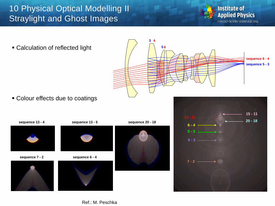
1. Surface scattering
1.1 Edge diffraction
1.2 Scattering at topological structures of surfaces
Dimensions: micro roughness – macroscopic ripple due to manufacturing errors
1.3 Scattering at single localized defects (contamination, micro defects)
perturbation of phase- and amplitude
2. Particle scattering :
2.1 Rayleigh regime , d << l
2.2 Theory of Rayleigh-Debye , d < l
2.3 Mie-scattering, spherical particles d > l
3. Volume scattering
3.1 Scattering at refractive index inhomogeneities,
atmospheric turbulence, striae in glass
3.2 Scattering at crystal boundaries (ceramic)
3.3 Scattering in statistical dense material/particle ensemble
biological tissue, multiple scattering events
10 Physical Optical Modelling II
Scattering Mechanisms

Geometry regular - statistical distributed
Single - multi scattering
Density of scatterers low - high, independence, saturation, change of illumination
Near - far field
Scaling, size of scatterers vs. wavelength, micro - macro
Coherence, scattering vs. re-emission
Polarization dependence
Discret scatterers vs. continuous n-variations
Absorption
Diffraction vs. geometrical approach
Steady state vs time dependence
Wavelength dispersion of material parameters
Finite volume size - boundary conditions
10 Physical Optical Modelling II
Aspects of Scattering

Geometry simplified
Boundaries simplified, mostly at infinity
Isotropic scattering characteristic
Perfect statistics of distributed particles
Multiple scattering neglected
Discretization of volume
Angle dependence of phase function simplified
Scattering centers independent
Scatterers point like objects
Spatially varying material parameters ignored
Field assumed to be scalar
Decoherence effects neglected
Absorption neglected
Interaction of scatterers neglected
l-dispersion of material data neglected
10 Physical Optical Modelling II
Approximations in Scattering Models
10 Physical Optical Modelling II
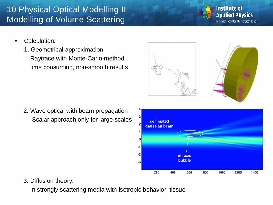
Modelling of Volume Scattering
Calculation:
1. Geometrical approximation:
Raytrace with Monte-Carlo-method
time consuming, non-smooth results
2. Wave optical with beam propagation
Scalar approach only for large scales
3. Diffusion theory:
In strongly scattering media with isotropic behavior; tissue
off axis
bubble
collimated
gaussian beam

Length scale below 1 cm:
Tatarski function due to
viscosity
PSD
Lengths scale up to 5 m:
Kolmogorov spectrum
PSD
Length scale above:
Karman spectrum
PSD
LogC
n2
(k)F
F --> const
Karman
large scale
Kolmogorov
inertial subrange
F =a k 311
F =a ek2
Viskose
Dissipation
Tatarski
k
kko iinner scaleouter scale
2
F ik
k
Ta eb
3
11
F kbTa
6
11
2
22 4
F
o
KaL
kb
10 Physical Optical Modelling II
Atmospheric Turbulence

Analytical solutions:
Spherical particles
1. generalized Lorentz-Mie theory, near and far field
2. multi sphere configurations
3. layered structures
Spheroids
Cylinders
1. single cylinders, with oblique incidence, near and far field
2. stacked cylinders
3. multi cylinder configurations, perpendicular incidence
Numerical solutions in time domain:
Arbitrary geometies
Finite difference time domain method (FDTD), only small volumes ( 2mm3), Dx = l/20
Pseudospectral method (PSTD) , Dx = l/4
Stationary solutions:
Discrete dipole approximation for arbitrary geomtries
T-matrix method
10 Physical Optical Modelling II
Available Solutions Maxwell Theory
Ref: A. Kienle
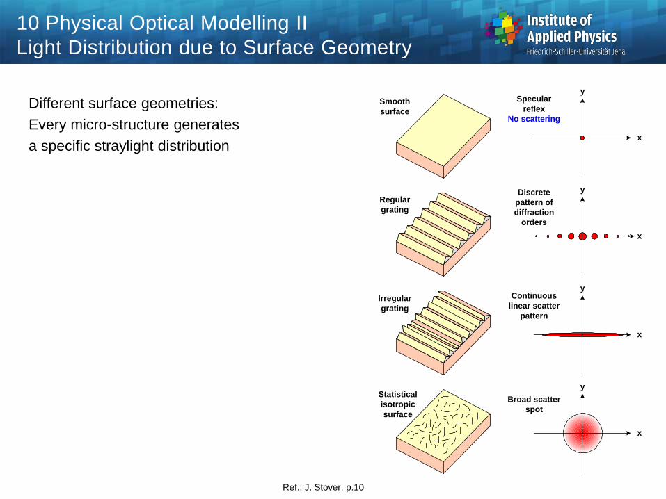
Different surface geometries:
Every micro-structure generates
a specific straylight distribution
10 Physical Optical Modelling II
Light Distribution due to Surface Geometry
x
y
Smooth
surface
Specular
reflex
No scattering
x
y
Regular
grating
Discrete
pattern of
diffraction
orders
x
y
Irregular
grating
Continuous
linear scatter
pattern
x
yStatistical
isotropic
surface
Broad scatter
spot
Ref.: J. Stover, p.10

Scattering at rough surfaces:
statistical distribution of light scattering
in the angle domain
Angle indicatrix of scattering:
- peak around the specular angle
- decay of larger angle distributions
depends on surface treatment
is
dP
dLog
q
qscattering angle
special polishing
Normal polishing
specular angle
10 Physical Optical Modelling II
Phenomenology of Surface Scattering
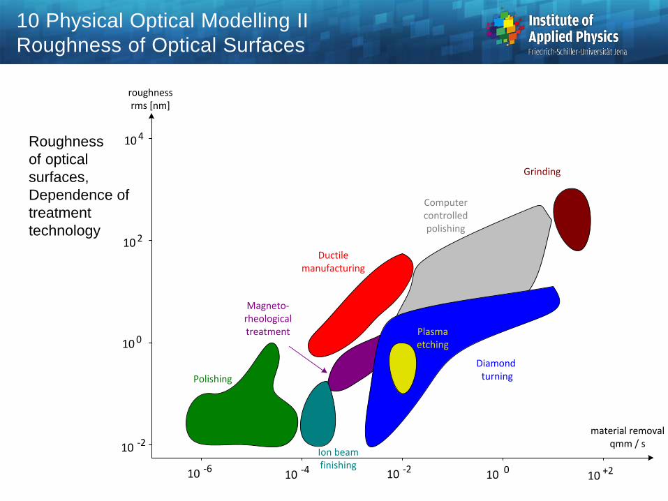
Roughness
of optical
surfaces,
Dependence of
treatment
technology
10 4
10 2
10 0
10 -2
10 -610 -4 10 -2 10 0
10 +2
Grinding
Polishing
Computercontrolledpolishing
Diamond turning
Plasmaetching
Ductilemanufacturing
Ion beam finishing
Magneto-rheological treatment
roughnessrms [nm]
material removalqmm / s
10 Physical Optical Modelling II
Roughness of Optical Surfaces

10 Physical Optical Modelling II
Surface Characterization
h(x)
x
C(Dx)
Dx
PSD(k)
k
A(k)
k
FFT FFT
| |2
< h1h
2 >
correlation
square
dxeyxhkA ikx
L
0
),()(
DD dxxxhxhL
xC )()(1
)(
topology
spectrum
autocorrelation
power spectral
density
2
)(1
)( dxexhL
kF ikx
PSD

10 Physical Optical Modelling II
Spatial Frequency of Surface Perturbations
Power spectral density of the perturbation
Three typical frequency ranges,
scaled by diameter D
1. Long range, figure error
deterministic description
resolution degradation
2. Mid frequency, critical
model description complicated
3. Micro roughness
statistical description
decrease of contrast
limiting lineslope m = -1.5...-2.5
log A2
Four
long range
low frequency
figure
Zernike
mid
frequencymicro
roughness
1/l
oscillation of
the polishing
machine
12/D1/D 40/D

Description of scattering characteristic of a surface: BSDF
(bidirectional scattering distribution function)
Straylight power into the solid angle dW
from the area element dA relative to
the incident power Pi
The BSDF works as the angle response
function
Special cases: formulation as convolution
integral
W
ddP
dP
dP
dLF
i
s
i
sBSDF
qcos
ndW
solid angle
areaelement
scattered power
dPs
normal
incidentpower
dPi
qi
sq
W iiiiiiBSDF dPFP qqqqq cos),(,,,),(
10 Physical Optical Modelling II
BSDF of a Surface

Exponential correlation
decay
PSD is Lorentzian function
Gaussian coerrelation
Fractal surface with
Hausdorf parameter D
K correlation model
parameter B, s
10 Physical Optical Modelling II
Model Functions of Surfaces
C x erms
x
c( )
2
F s
sPSD
rms c
c
( )
1
1
2
2
C x erms
x
c( )
2
1
2
2
F s ePSD
c rms
s c
( )
2
2
4
2
F s
n
n
K
sPSD
n
n( )
1
2
21
2 2
1
F s
A
s BPSD C
( )/
12
2
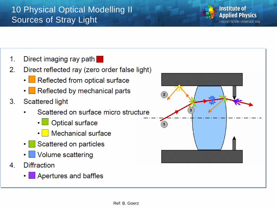
10 Physical Optical Modelling II
Sources of Stray Light
Ref: B. Goerz
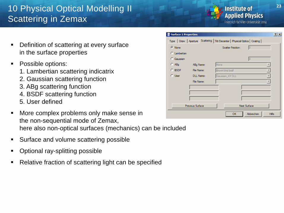
Definition of scattering at every surface
in the surface properties
Possible options:
1. Lambertian scattering indicatrix
2. Gaussian scattering function
3. ABg scattering function
4. BSDF scattering function
5. User defined
More complex problems only make sense in
the non-sequential mode of Zemax,
here also non-optical surfaces (mechanics) can be included
Surface and volume scattering possible
Optional ray-splitting possible
Relative fraction of scattering light can be specified
23 10 Physical Optical Modelling II
Scattering in Zemax

Surface scattering:
Projection of the scattered ray on the surface, difference x to the specular ray: x
Volumne scattering:
Angle scattering description by probability P
Lambertian scattering:
isotropic
Gaussian scattering
ABg model scatter
Henyey-Greenstein volume scattering
(biological tissue model)
Rayleigh scattering
10 Physical Optical Modelling II
Scattering in Zemax
2
2
)(
x
BSDF eAxF
gBSDFxB
AxF
)(
2/32
2
cos214
1)(
gg
gP
ql
q 2
4cos1
8
3)( P

Data file with scattering functions: ABg-data.dat
File can be edited
25 10 Physical Optical Modelling II
Scattering in Zemax

Tools / Catalogs / ABg Scatter Data Catalogs
Specification and definition of scattering
parameters:
wavelength, angle, A, B, g
Tools / Catalogs / SCatter Function Viewer
Graphical representation of the scattering function
26 10 Physical Optical Modelling II
Scattering in Zemax
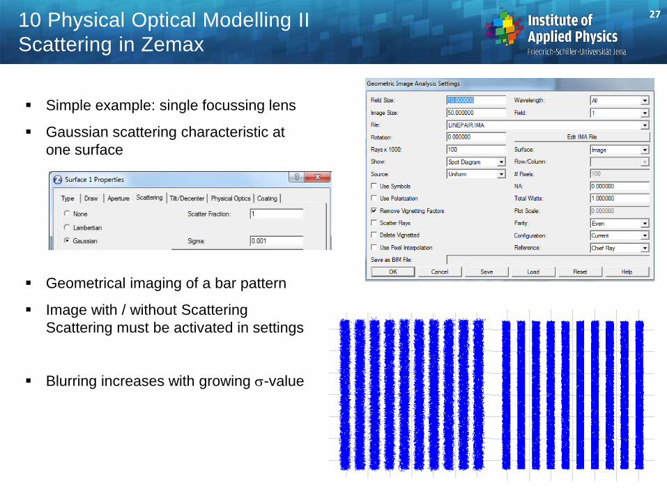
Simple example: single focussing lens
Gaussian scattering characteristic at
one surface
Geometrical imaging of a bar pattern
Image with / without Scattering
Scattering must be activated in settings
Blurring increases with growing -value
27 10 Physical Optical Modelling II
Scattering in Zemax

Example from samples with non-sequential mode
Important sampling accelerates the calculation
28 10 Physical Optical Modelling II
Scattering in Zemax
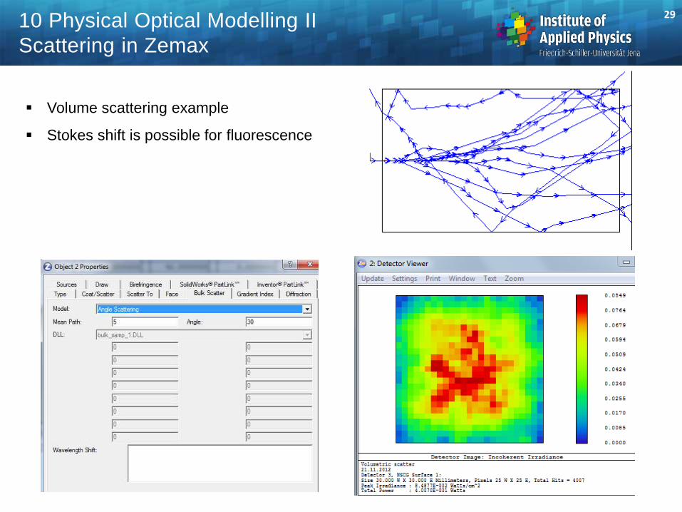
Volume scattering example
Stokes shift is possible for fluorescence
29 10 Physical Optical Modelling II
Scattering in Zemax

Fresnel Formulas
n n'
incidence
reflection transmission
interface
E
B
i
i
E
B
r
r
E
Bt
t
normal to the interface
i
i'i
a) s-polarization
n n'
incidence
reflection
transmission
interface
B
E
i
i
B
E
r
r
B
E t
t
normal to the interface
i'i
i
b) p-polarization
Schematical illustration of the ray refraction ( reflection at an interface
The cases of s- and p-polarization must be distinguished
30

Fresnel Formulas
Electrical transverse polarization
TE, s- or -polarization, E perpendicular to incidence plane
Magnetical transverse polarization
TM, p- or p-polarization, E in incidence plane
Boundary condition of Maxwell equations
at a dielectric interface:
continuous tangential component of E-field
Amplitude coefficients for
reflected field
transmitted field
Reflectivity and transmission
of light power
TEe
rTE
E
Er
1 TE
TEe
tTE r
E
Et 1
' TMTM r
n
nt
nn EE 2211
tt EE 21
TMe
rTM
E
Er
2rP
PR
e
r 2
cos
'cos't
in
in
P
PT
e
t
||
31

Fresnel Formulas: Stokes Relations
1 rt
1cos
'cos|||| r
i
it
Relation between the amplitude coefficients for reflection/transmission:
1. s-components:
field components additive
minus sign due to phase jump
2. p-components:
energy preservation but change of
area size due to projection,
correction factor, no additivity of
intensities
field
amplitudes
incidence reflection
transmission
Ei
Er
Et
cross section
area
continuous
tangential
component
32
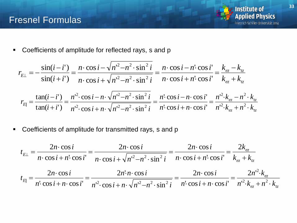
Fresnel Formulas
Coefficients of amplitude for reflected rays, s and p
Coefficients of amplitude for transmitted rays, s and p
tzez
tzezE
kk
kk
inin
inin
innin
innin
ii
iir
'cos'cos
'cos'cos
sin'cos
sin'cos
)'sin(
)'sin(
222
222
tzez
tzezE
knkn
knkn
inin
inin
innnin
innnin
ii
iir
22
22
2222
2222
||'
'
'coscos'
'coscos'
sin'cos'
sin'cos'
)'tan(
)'tan(
tzez
ezE
kk
k
inin
in
innin
in
inin
int
2
'cos'cos
cos2
sin'cos
cos2
'cos'cos
cos2
222
tzez
ezE
knkn
kn
inin
in
innnin
inn
inin
int
22
2
2222||
'
'2
'coscos'
cos2
sin'cos'
cos'2
'coscos'
cos2
33

Fresnel Formulas
Typical behavior of the Fresnel amplitude coefficients as a function of the incidence angle
for a fixed combination of refractive indices
i = 0
Transmission independent
on polarization
Reflected p-rays without
phase jump
Reflected s-rays with
phase jump of
(corresponds to r<0)
i = 90°
No transmission possible
Reflected light independent
on polarization
Brewster angle:
completely s-polarized
reflected light
r
r
t
t
i
Brewster
34

Fresnel Formulas: Energy vs. Intensity
Fresnel formulas, different representations:
1. Amplitude coefficients, with sign
2. Intensity cefficients: no additivity due to area projection
3. Power coefficients: additivity due to energy preservation
r , t
0 10 20 30 40 50 60 70 80 90-1
-0.8
-0.6
-0.4
-0.2
0
0.2
0.4
0.6
0.8
1
i
t
r
r
t
R , T
i0 10 20 30 40 50 60 70 80 90
0
0.1
0.2
0.3
0.4
0.5
0.6
0.7
0.8
0.9
1
T(In)
T(In)
R(In)
R(In)
R , T
i0 10 20 30 40 50 60 70 80 90
0
0.1
0.2
0.3
0.4
0.5
0.6
0.7
0.8
0.9
1
T
T
R
R
35

Fresnel Formulas
Reflectivity and transmittivity of power
Arbitrary azimuthal angle of polarization: decompositioin of components
In case of vanishing absorption:
Energy preservation
Special case of normal incidence
Typical values for some glasses and optical materials in air
)'(sin
)'(sin2
2
ii
iiR
)'(tan
)'(tan2
2
||ii
iiR
)'(sin
2cos'2sin2 ii
iiT
)'(cos)'(sin
'2sin2cos22||
iiii
iiT
ee RRR 22
|| sincos ee TTT 22
|| sincos
1TR
2
'
'
nn
nnR
2'
'4
nn
nnT
n R
1.4 2.778 %
1.5 4.0 %
1.8 8.16 %
2.4 16.96 %
36
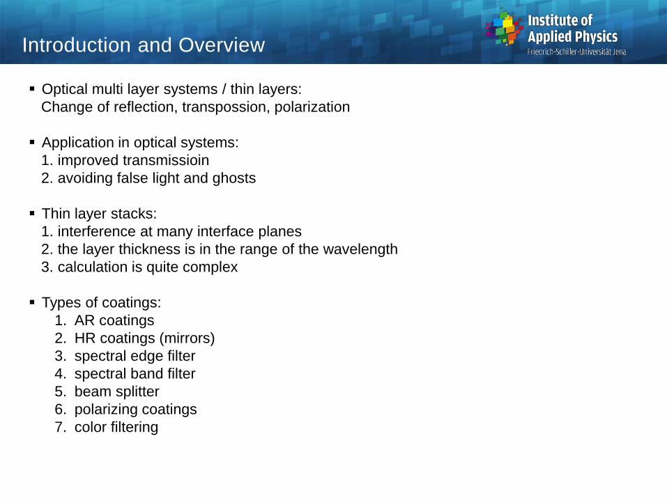
Optical multi layer systems / thin layers:
Change of reflection, transpossion, polarization
Application in optical systems:
1. improved transmissioin
2. avoiding false light and ghosts
Thin layer stacks:
1. interference at many interface planes
2. the layer thickness is in the range of the wavelength
3. calculation is quite complex
Types of coatings:
1. AR coatings
2. HR coatings (mirrors)
3. spectral edge filter
4. spectral band filter
5. beam splitter
6. polarizing coatings
7. color filtering
Introduction and Overview

Types of Coatings
T
l
selective
filter
positive
T
l
selective
filter
negative
R
l
polarization
beam splitter
p s
T
l
band pass
filter
T
l
edge filter
low pass
T
l
edge filter
high pass
R
l
AR coating
R
l
HR coating
R
l
broadband
beam splitter

Comparison of coatings with different number of layers:
1. without coating
2. single layer
3. double layer
4. multi-layer
Comparison of Coatings
l
5
4
3
2
1
0
400 500 600 700 800 900
R in %
uncoated
mono layer
coating
double layer
coating
multi layer
coating

Principle of calculation of a thin layer system:
1. decomposition of field components at the plane interfaces
2. continuity condition of Fresnel equations
3. resulting matrix of layer sequence
4. calculation of th eigenwert values
sspp eEeEE
sspp eHeHH
EenH k
0
0
m
Field Components in Layers
y
z
x
Es
Ep
E
Ers
Etp
Ets
Etp
Et
Er
q
q q'
incidence
plane
incident
reflected
transmitted
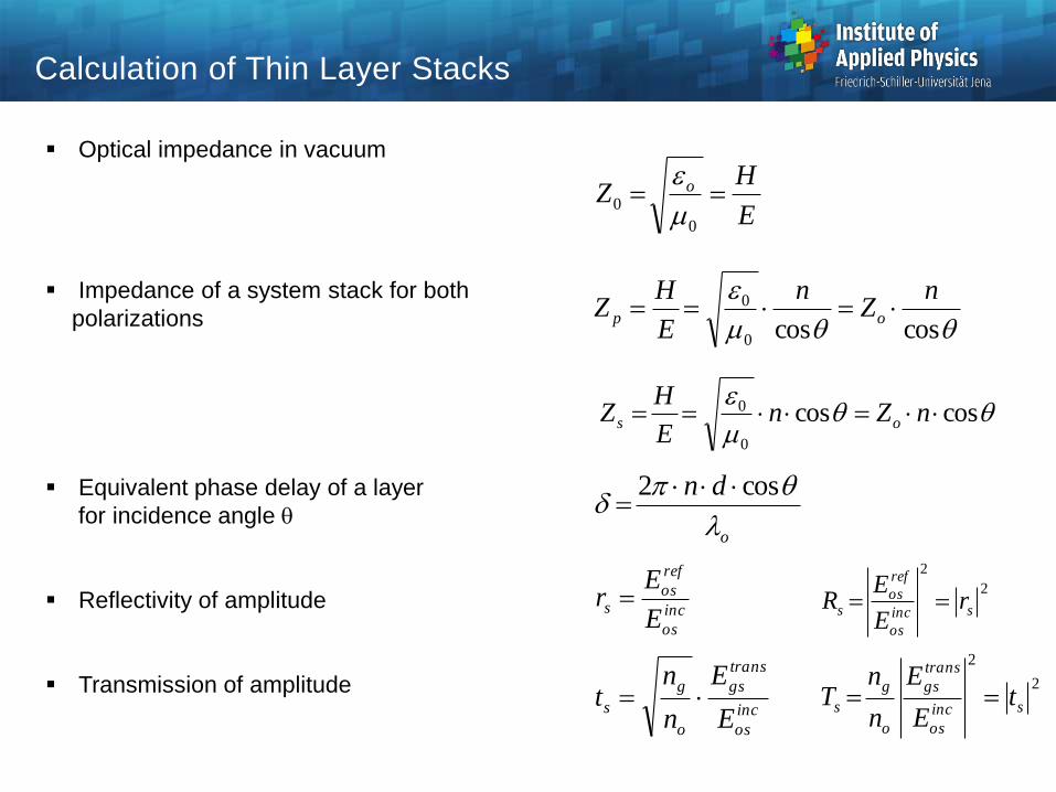
Optical impedance in vacuum
Impedance of a system stack for both
polarizations
Equivalent phase delay of a layer
for incidence angle q
Reflectivity of amplitude
Transmission of amplitude
E
HZ o
0
0m
qqm
coscos0
0 nZ
n
E
HZ op
qqm
coscos
0
0 nZnE
HZ os
o
dn
l
q
cos2
inc
os
ref
oss
E
Er
2
2
sinc
os
ref
oss r
E
ER
inc
os
trans
gs
o
g
sE
E
n
nt
2
2
sinc
os
trans
gs
o
g
s tE
E
n
nT
Calculation of Thin Layer Stacks

Field components:
1. entrance and exit of a layer
2. E and H-field
3. forward and backward
propagating wave
4. both polarization components
Continuity conditions at the interface
planes
Solution of linear system equations
Also valid for absorbing media
Matrix Model of Stack Calculation
d1
n0
n1
ng
Ei0 Er0
Eg
Luft
Layer No 1
substrate
d2n2
dj-1nj-1
djnj
dj+1nj+1
dmnm
q1
q2
qj-1
qj
qj+1
qm
q0
qg
Layer No j-1
Layer No 2
Layer No
m
Layer No j
Layer No j+1
Ejt- Ejr-
Ejr+Ejt+
Ej-1,t+
Ej-1,t- Ej-1,r-
Ej-1,r+
Ej+1,t+
Ej+1,t- Ej+1,r-
Ej+1,r+

Transfer matrices
- for one layer
- for both polarizations
p and s
Matrix of complete stack
(representation with B)
Impedance of air and substrate
must be taken into account
sj
sj
jjjj
j
jj
j
sj
sj
H
E
ni
n
i
H
E
,
,
,1
,1
cossincos
sincos
cos
q
q
pj
pj
jj
j
j
j
jj
j
pj
pj
H
E
ni
n
i
H
E
,
,
,1
,1
cossincos
sincos
cos
q
q
m
m
jm
j
j
B
EM
B
E
1231,1 ... MMMMMMM mmjm
ggo
gs nZ qm
cos
0
qm
cos0
0
0 nZ os
Transfer Matrices

Single layer matrix
Reflectivity of complete system
for s and p polarization
Transmission of complete system
for s and p polarization
Matrix approach:
- analysis method
- optimization by NLSQ-algorithms
- problem: periodicity of phase
In principle solution only for
1. one wavelength
2. one incidence angle
Typically the spectral performance is shown as a function of lo / l
2221
1211
cossin
sincos
MM
MM
Zi
Z
i
M
jjj
j
j
j
j
22211211
22211211
MZMMZZMZ
MZMMZZMZr
sgsgsoso
sgsgsoso
s
22211211
2
MZMMZZMZ
Zt
sgsgsoso
sos
Final Calculations Step

Periodicity of phase:
dependence of performance on thickness
Period is the wavelength
Special thicknesses:
waves in phase,
no effect of the thin layer
stack
Influence of the Layer Thickness
R
0 1 2 3 4 5 6 7 8 90
0.05
0.1
0.15
0.2
0.25
0.3
0.35
0.4
nl = 2.30
nl = 1.70
nl = 1.50
nl = 1.35
nl = 1.22

Fresnel formulas:
reflectivity in general depends on
1. incidence angle
2. polarization
Degredation for broad band
and incidence angle interval
i
l / l o
lDesign
iDesign
R = 0.1
R = 0.0
R = 0.2
R = 0.3
R = 0.4
R = 0.4
R = 0.5
R = 0.5
R = 0.6R = 0.6
R = 0.7
Dependence on Incidence Angle and Polarization
s-polarization
p-polarization
total
R in %
i in °

Special example:
13 layer with
L : n = 1.45
H : n = 2.35
Example Coating
R
0.4 0.6 0.8 1 1.2 1.4 1.60
0.1
0.2
0.3
0.4
0.5
0.6
0.7
0.8
0.9
1
i = 20° p
i = 20° s
i = 30° p
i = 30° s
l / l
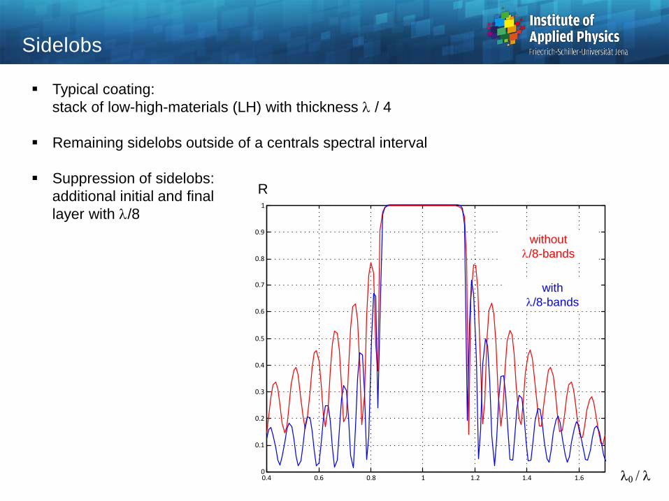
Typical coating:
stack of low-high-materials (LH) with thickness l / 4
Remaining sidelobs outside of a centrals spectral interval
Suppression of sidelobs:
additional initial and final
layer with l/8
Sidelobs
R
l / l0.4 0.6 0.8 1 1.2 1.4 1.60
0.1
0.2
0.3
0.4
0.5
0.6
0.7
0.8
0.9
1
without
l/8-bands
with
l/8-bands

Example Coating
R
l /l 0.4 0.6 0.8 1 1.2 1.4 1.6
0
0.005
0.01
0.015
0.02
0.025
0.03
0.035
0.04
0.045
0.05
i = 0°
i = 10°
i = 20°
i = 40°
i = 30°
Special example:
4 layer with thickness l/4
L : n = 1.45
H : n = 2.35
Reflectivity for different
incidence angles
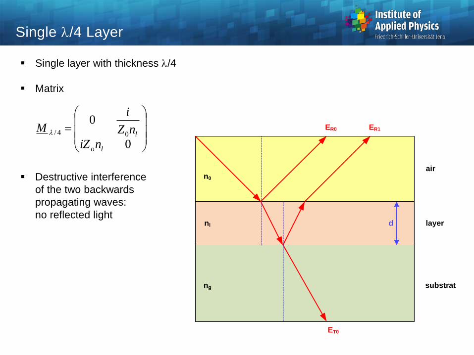
Single layer with thickness l/4
Matrix
Destructive interference
of the two backwards
propagating waves:
no reflected light
0
004/
lo
l
niZ
nZ
i
M l
Single l/4 Layer
d
n0
nl
ng
ER0 ER1
ET0
air
layer
substrat

Reflectivity of amplitude
Phase condition
corresponds to l/4
Amplitude condition:
identical amplitude
Problem:
on a glass with n = 1.5
a layermaterial of
n=1.23 is needed
lnd
4
l
gol nnn
sincos
sincos2
2
innnnnn
innnnnnr
lgogol
lgogol
Single l/4 Layer
l / 4
no nl ng
air layer substrat
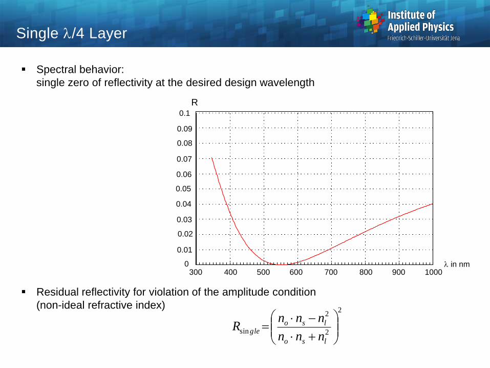
Spectral behavior:
single zero of reflectivity at the desired design wavelength
Residual reflectivity for violation of the amplitude condition
(non-ideal refractive index) 2
2
2
sin
lso
lsogle
nnn
nnnR
Single l/4 Layer
R0.1
0.05
0.01
0
0.02
0.03
0.04
0.06
0.07
0.08
0.09
l in nm300 400 500 600 700 800 900 1000

Double layer: several solutions possible
One simple solution: thickness
Corresponding amplitude condition
Residual reflectivity
2
2
1
2
20
2
1
2
20
nnnn
nnnnR
g
g
double
4/2211 l dndn
g
o
n
n
n
n
2
1
Double Layer
d1
d2
n0
n1
n2
ns
ER0 ER1 ER2
ET0
air
layer 1
layer 2
substrat

Scheme:
Typical broad spectral performance
for reflectivity
Multi Layer
n2
substrat
n3
n4
n5
n6
n7
n8
n1 air
R0.1
0.05
0.01
0
0.02
0.03
0.04
0.06
0.07
0.08
0.09
l in nm300 400 500 600 700 800 900 1000
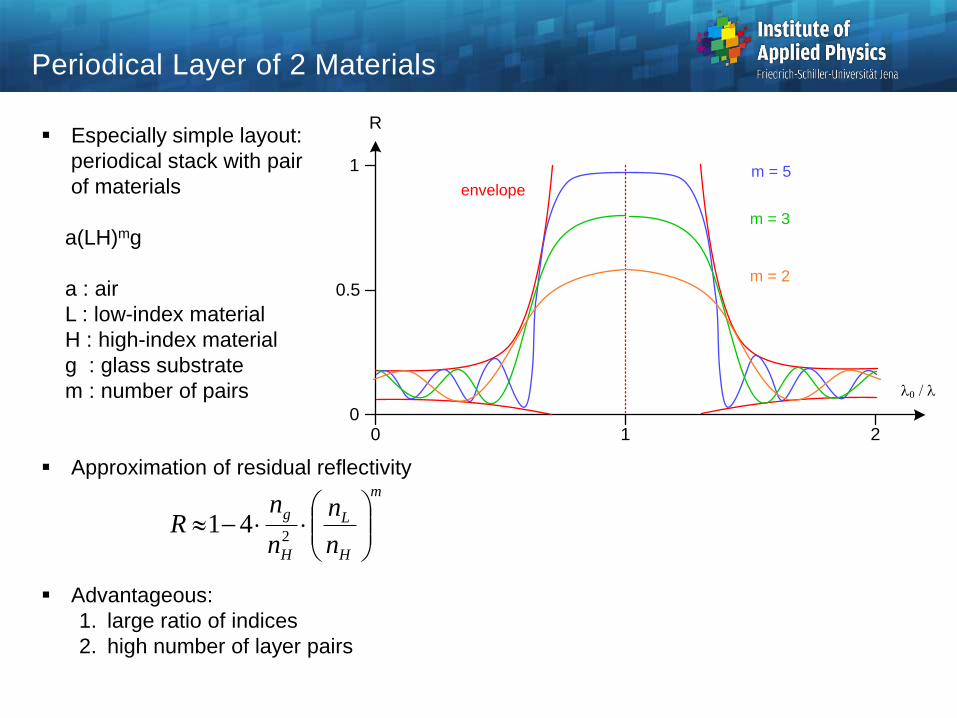
Especially simple layout:
periodical stack with pair
of materials
a(LH)mg
a : air
L : low-index material
H : high-index material
g : glass substrate
m : number of pairs
Approximation of residual reflectivity
Advantageous:
1. large ratio of indices
2. high number of layer pairs
m
H
L
H
g
n
n
n
nR
241
Periodical Layer of 2 Materials
l / l
R
1
00 1 2
0.5
envelope
m = 5
m = 3
m = 2

Comfortable choice:
layer thickness l/4
Peak reflectivity
Spectral width of the reflectivity
interval:
growing with increased n-ratio
2
2
2
max
m
H
L
g
o
m
H
L
g
o
n
n
n
n
n
n
n
n
R
Periodical Layer of 2 Materials
nH / nL
Dl / l
1 1.5 2 2.5 3 3.5 40
0.1
0.2
0.3
0.4
0.5
0.6
0.7
0.8
0.9
1
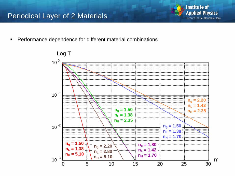
Performance dependence for different material combinations
Periodical Layer of 2 Materials
m0 5 10 15 20 25 30
10-3
10-2
10-1
100
Log T
ng = 1.50
nL = 1.38
nH = 1.70
ng = 1.50
nL = 1.38
nH = 5.10
ng = 1.50
nL = 1.38
nH = 2.35
ng = 2.20
nL = 1.42
nH = 2.35
ng = 1.80
nL = 1.42
nH = 1.70
ng = 2.20
nL = 2.80
nH = 5.10

Combination of layers with real refractive indices can be used to generate arteficial indices
Equivalent Layers
d = l / 4 n = 1.62
n = 2.15
n = 1.38
d = l / 2
d = l / 4
n = 1.38
n = 1.35
n = 2.35
n = 2.35
d = l / 4
d = l / 4
no = 1
d = l / 2
ns = 1.52
n = 1.38
n = 2.35
n = 1.38
ideal equivalent

Graphical visualization of thin layer effects in the complex impedance plane
Every layer is represented by an arc
The arc length corresponds to the phase
Absorbing materilals are represented by spiral curves
Initial and final point must be on the real axis
Exception:metals with complex substrate index
Impedance Diagram
Re Y
Im Y
1 3 42
Layer 1
n = 2.35
Layer 2
n = 1.35
1.52
0.5016 3.633
-1.50
+1.0
Re Y
Im Y
1 3 42
no ng
solution 1
solution 2

Graphical illustration of layer stacks in the complex plane of the reflectivities
Every layer is represented by an arrow with
1. length, corresponds to amplitude
2. direction, corresponds to phase
Im(r)
Re(r)r
1 r2
rres
r'2
r''2
r'res
r''res
Reflectivity Diagram
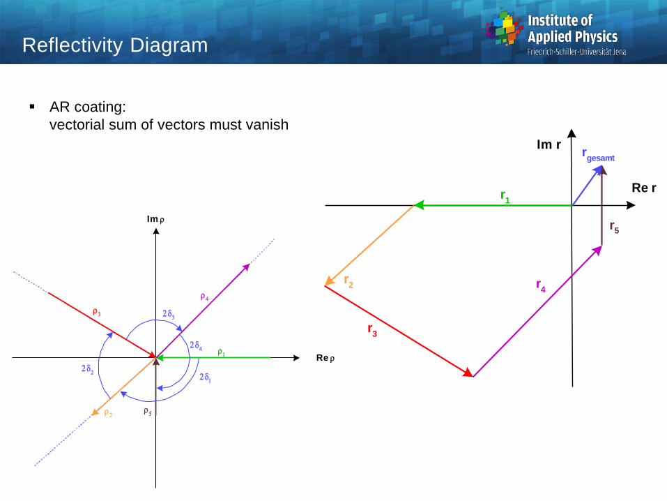
AR coating:
vectorial sum of vectors must vanish
Re r
Im r
r1
r2
r3
r4
r5
rgesamt
Reflectivity Diagram
Re
Im

Material Typ Refractive
index n
Spectral
range
Magnesiumfluorid L 1.38 UV - nIR
Cerfluorid L 1.62
Aluminiumoxid 1.62 UV - nIR
Cryolite 1.35 UV - nIR
Siliziumdioxid 1.48
Magnesiumoxid L 1.72
Zirkonium Dioxid H 2.00 UV - nIR
Hafniumdioxid H 1.98
Titandioxid H 2.45 vis - nIR
Zinksulfid H 2.30 vis - nIR
Cerdioxid 2.20 vis - nIR
Thoriumfluorid 1.52 UV - nIR
Silizium Monoxid 1.95 vis - nIR
Silizium 3.50 nIR - IR
Germanium 4.20 nIR - IR
Zinkselenid 2.44 nIR - IR
Cadmiumtellurid 2.69 nIR - IR
Bleitellurid 5.5 IR
Tellur H 4.80
Lithiumfluorid L 1.37
Coating Materials

Multi-beam interference analogous to the Fabry-Perot
Extrem narrow spectral transmission
Calculation of transmission:
Airy formula
cos21
)1(2
2
RR
RIT
Interference Coating
T
F-0.4 -0.3 -0.2 -0.1 0 0.1 0.2 0.3 0.40
0.1
0.2
0.3
0.4
0.5
0.6
0.7
0.8
0.9
1
R = 0.900
R = 0.950
R = 0.980
R = 0.990
R = 0.999

Transmission in Optical Systems
Residual reflectivity of the (identical) surfaces in an optical system with n surfaces:
Overall transmission of energy:
Transmission decreases
nonlinear
Practical consequences:
1. loss of signal energy
2. contrast reduction in
case of imaging
3.occurence of ghost images
n0 10 20 30 40 50 60
0
0.1
0.2
0.3
0.4
0.5
0.6
0.7
0.8
0.9
1
T
R = 1 %
R = 2 %
R = 4 %
R = 6 %R = 10 %
n
ges RT 1
64
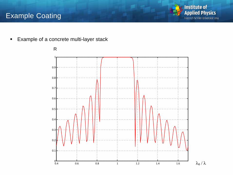
Example of a concrete multi-layer stack
Example Coating
R
l / l0.4 0.6 0.8 1 1.2 1.4 1.60
0.1
0.2
0.3
0.4
0.5
0.6
0.7
0.8
0.9
1
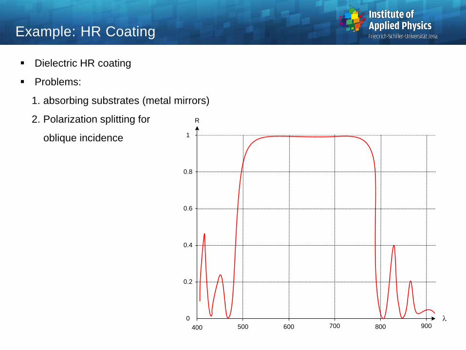
Dielectric HR coating
Problems:
1. absorbing substrates (metal mirrors)
2. Polarization splitting for
oblique incidence
Example: HR Coating
l
1
0.8
0.6
0.4
0.2
0
400 500 600 700 800 900
R

Requirements:
1. steep edge
2. high reflectivity R on one side
3. high transmission T on
the other side
4. no oscillations
Application:
cold mirror, blocking of
infrared light
Thin Layer as Edge Filter
l
1
0.8
0.6
0.4
0.2
0
400 600 800 1000 1200 1400
T in %
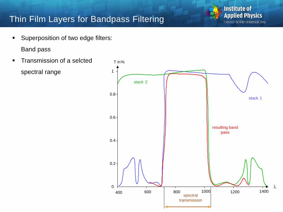
Superposition of two edge filters:
Band pass
Transmission of a selcted
spectral range
Thin Film Layers for Bandpass Filtering
l
1
0.8
0.6
0.4
0.2
0
400 600 800 1000 1200 1400
T in %
stack 1
stack 2
resulting band
pass
spectral
transmission

Special coloring properties by spectral filtering
Example application:
selective spectral transmission
for subtractive color printing
Color Filtering
l
1.0
0.75
0.50
0.25
0
300 400 500 600 700
T in %
yellow magenta cyan
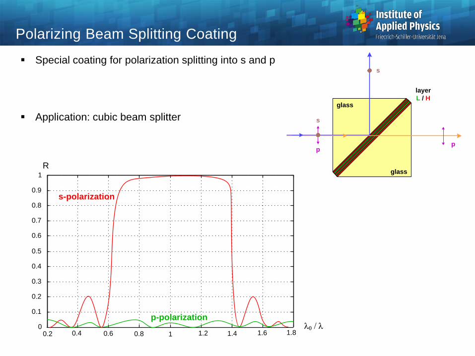
Special coating for polarization splitting into s and p
Application: cubic beam splitter
Polarizing Beam Splitting Coating
layer
L / H
pp
s
s
glass
glass
R
l / l1 1.20.80.6 1.4 1.60.4 1.80.2
s-polarization
p-polarization0
0.1
0.2
0.3
0.4
0.5
0.6
0.7
0.8
0.9
1
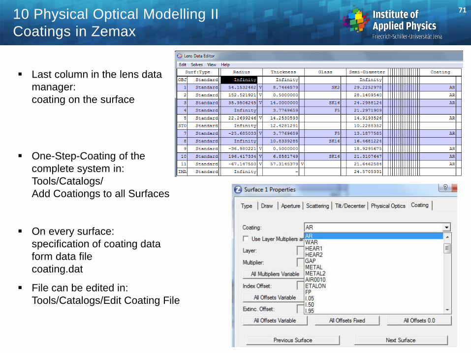
Last column in the lens data
manager:
coating on the surface
One-Step-Coating of the
complete system in:
Tools/Catalogs/
Add Coationgs to all Surfaces
On every surface:
specification of coating data
form data file
coating.dat
File can be edited in:
Tools/Catalogs/Edit Coating File
71 10 Physical Optical Modelling II
Coatings in Zemax

Syntax of the coating file,
Tools/Catalogs/Coating Listing
1. Material specifications:
different indices of the substrate
2. coatings:
all layers: material, thickness in waves
material must be given
3. ideal coatings:
described by transmission value
4. coatings specified by table
explicite values of Rs, Rp, Ts, Tp for each
wavelength and incidence angle
5. encripted coatings
(binary format)
72 10 Physical Optical Modelling II
Coatings in Zemax
MATE BK7
0.4 1.5308485 0
0.46 1.5244335 0
0.5 1.5214145 0
0.7 1.5130640 0
0.8 1.5107762 0
1.0 1.5075022 0
2.0 1.4945016 0
COAT AR
MGF2 .25
COAT HEAR1
MGF2 .25
ZRO2 .50
CEF3 .25
COAT I.05
COAT I.50
COAT I.95
TABLE PASS45
ANGL 0.0
WAVE 0.55 1.0 1.0 0.0 0.0 0.0 0.0 0.0 0.0
ANGL 45.0
WAVE 0.55 0.0 0.0 1.0 1.0 0.0 0.0 0.0 0.0
ANGL 90.0
WAVE 0.55 1.0 1.0 0.0 0.0 0.0 0.0 0.0 0.0
ENCRYPTED ZEC_HEA673
ENCRYPTED VISNIR
ENCRYPTED ZEC_UVVIS
ENCRYPTED ZEC_HEA613
COAT CZ2301,45
MGF2_G 0.08450000 1 0
XIV 0.02640000 1 0
MGF2_G 0.01280000 1 0
XIV 0.07600000 1 0
MGF2_G 0.01380000 1 0
XIV 0.02930000 1 0
MGF2_G 0.03260000 1 0
XIV 0.01070000 1 0

Selection of coating/polarization analysis
Tapering of coatings is possible:
radial polynomial of cosine-shaped
spatial thickness variation
Import of professional coating software
data is possible
Given coatings can be incorporated into the
optimization to a certain flexibility
- thickness scaling
- offset of refractive index
- offset of extinction coefficient
73 10 Physical Optical Modelling II
Coatings in Zemax

Detailed polarization analyses are possible at the individual surfaces by using the coating
menue options
9 Physical Optical Modelling I
Coating Analysis in Zemax