OPTICAL CHARACTERIZATION OF NON-IMAGINGeprints.utar.edu.my/2375/2/EGA-2016-1102576-1.pdf · 2.3.1...

OPTICAL CHARACTERIZATION OF NON-IMAGING DISH CONCENTRATOR FOR OPTIMIZING

INTERCONNECTION OF SOLAR CELLS IN DENSE ARRAY CONCENTRATOR PHOTOVOLTAIC SYSTEM

WONG CHEE WOON

DOCTOR OF PHILOSOPHY IN ENGINEERING

LEE KONG CHIAN FACULTY OF ENGINEERING AND SCIENCE

UNIVERSITI TUNKU ABDUL RAHMAN OCTOBER 2016

OPTICAL CHARACTERIZATION OF NON-IMAGING DISH

CONCENTRATOR FOR OPTIMIZING INTERCONNECTION OF

SOLAR CELLS IN DENSE ARRAY CONCENTRATOR

PHOTOVOLTAIC SYSTEM

By

WONG CHEE WOON

A thesis submitted to the Department of Electrical and Electronic Engineering,

Lee Kong Chian Faculty of Engineering and Science,

Universiti Tunku Abdul Rahman,

in partial fulfillment of the requirements for the degree of

Doctor of Philosophy in Engineering

October 2016

ii

ABSTRACT


CONCENTRATOR FOR OPTIMIZING INTERCONNECTION OF

SOLAR CELLS IN DENSE ARRAY CONCENTRATOR

PHOTOVOLTAIC SYSTEM

Wong Chee Woon

Non-uniform solar illumination is one of the key factors that severely restrains

electrical performance for the dense array concentrator photovoltaic (DACPV)

module consisted of multi-junction solar cells in serial and parallel connection.

The non-uniform illumination can cause the DACPV module to encounter

significant deterioration in output power due to the current mismatch problem.

Addressing this issue, a comprehensive study to optimize the electrical

performance of DACPV system comprised of the non-imaging dish

concentrator (NIDC) prototype is proposed. A numerical simulation has been

developed to analyze the optical characteristics of NIDC by considering

imperfection factors, i.e. circumsolar radiation, slope error, and optical

misalignment. The simulated results are very useful for the designer to optimize

the size of the receiver. From the simulated results, the author can conclude that

the three imperfection factors can cause serious deterioration to the uniform

illumination distributed on solar cells. Based on the simulated flux distribution,

a systematic methodology to optimize the layout configuration of solar cells

interconnection circuit in DACPV module has been proposed by minimizing the

current mismatch caused by non-uniformity of concentrated sunlight. An

iii

optimized layout of interconnection solar cells circuit with a minimum power

loss of 6.5% can be achieved by minimizing the effects of imperfection factors.

Last but not least, a high concentrated solar flux scanner has been designed and

constructed to acquire flux distribution of the NIDC prototype. The scanner is

capable of acquiring high concentrated solar flux distribution up to 1182 suns

accurately and rapidly using an array of triple-junction solar cells. A systematic

technique has been proposed to analyze the amount of imperfection factors for

the NIDC prototype: mirror reflectivity of 0.93, slope error of 3 mrad,

circumsolar ratio of 0.1, and optical misalignment angles of 0.2.

iv

ACKNOWLEDGEMENT

First and foremost, I would like to take this opportunity to express my sincere

appreciation and deepest gratitude to my supervisor, Prof. Dr. Chong Kok

Keong, for his guidance, invaluable advice, understanding and considerations

on my works. I am able to gain many experiences, skills and knowledge from

him.

I wish to express my gratitude to Dr. Lau Sing Liong, my co-supervisor. He had

provided me continuous guidance, directions and advice when I was conducting

my works. I would also wish to indicate special gratitude and deepest

thankfulness to my research’s partners, Siaw Fei Lu, Yew Tiong Keat, Tan Ming

Hui and Tan Woei Chong, for their assistances. Furthermore, I would like to

appreciate to none forgetting all of the lab officers and lab assistants, especially

Mr. Ho Kok Wai. They always give me support, encouragement, advice,

technical expertise and experiences.

To my beloved family, appreciate for the encouragement and mentally support

throughout the duration of my study. Last but not the least, with sincere affection

and love to my friends, thank you for your friendship, constant encouragement

and invaluable help, I wish you all great blessing.

v

APPROVAL SHEET

This thesis entitled “OPTICAL CHARACTERIZATION OF NON-

IMAGING DISH CONCENTRATOR FOR OPTIMIZING

INTERCONNECTION OF SOLAR CELLS IN DENSE ARRAY

CONCENTRATOR PHOTOVOLTAIC SYSTEM” was prepared by WONG

CHEE WOON and submitted as partial fulfillment of the requirements for the

degree of Doctor of Philosophy in Engineering at Universiti Tunku Abdul

Rahman.

Approved by:

___________________________

(Prof. Dr. Chong Kok Keong)

Date:…………………..

Supervisor

Department of Electrical and Electronic Engineering

Lee Kong Chian Faculty of Engineering and Science

Universiti Tunku Abdul Rahman

___________________________

(Dr. Lau Sing Liong)

Date:…………………..

Co-supervisor

Department of Electrical and Electronic Engineering

Lee Kong Chian Faculty of Engineering and Science

Universiti Tunku Abdul Rahman

vi

LEE KONG CHIAN FACULTY OF ENGINEERING AND SCIENCE

UNIVERSITI TUNKU ABDUL RAHMAN

Date: 7 October 2016

SUBMISSION OF THESIS

It is hereby certified that WONG CHEE WOON (ID No: 11UED02576) has

completed this thesis entitled “OPTICAL CHARACTERIZATION OF NON-

IMAGING DISH CONCENTRATOR FOR OPTIMIZING

INTERCONNECTION OF SOLAR CELLS IN DENSE ARRAY

CONCENTRATOR PHOTOVOLTAIC SYSTEM” under the supervision of

Prof. Dr. CHONG KOK KEONG (Supervisor) from the Department of Electrical

and Engineering, Lee Kong Chian Faculty of Engineering and Science, and Dr.

LAU SING LIONG (Co-Supervisor) from the Department of Electrical and

Engineering, Lee Kong Chian Faculty of Engineering and Science.

I understand that University will upload softcopy of my thesis in pdf format into

UTAR Institutional Repository, which may be made accessible to UTAR community

and public.

Yours truly,

____________________

(Wong Chee Woon)

vii

DECLARATION

I hereby declare that the dissertation is based on my original work except for

quotations and citations which have been duly acknowledged. I also declare that

it has not been previously or concurrently submitted for any other degree at

UTAR or other institutions.

Name: Wong Chee Woon

Date: 7 October 2016

viii

TABLE OF CONTENTS

Page

ABSTRACT ii

ACKNOWLEDGEMENT iv

APPROVAL SHEET v

SUBMISSION OF THESIS vi

DECLARATION vii

TABLE OF CONTENTS viii

LIST OF TABLES x

LIST OF FIGURES xi

LIST OF ABBREVIATIONS xvii

CHAPTER

1.0 INTRODUCTION 1 1.1 Research Background and Motivation 1

1.2 The Challenges 3

1.3 Objectives 4

1.4 Contributions 5

1.5 Outline of the Thesis 7

1.6 Publications 9

2.0 LITERATURE REVIEW 10

2.1 Introduction 10

2.2 Effects of Non-Uniform Illumination in CPV System 10

2.3 Optical Design of Solar Concentrators 12

2.3.1 Parabolic Dish Concentrator 13

2.3.2 Fresnel Concentrator 15

2.3.3 Non-Imaging Planar Concentrator 17

2.4 Non-Conventional Solar Cells 19

2.4.1 Radial Solar Cells Receiver 20

2.4.2 Solar Cells with Different Geometries 21

2.4.3 High-Voltage Solar Cells 22

2.5 Techniques to Measure Solar Flux Distribution 23

2.5.1 Direct Measurement Method 23

2.5.2 Indirect Measurement Method 25

3.0 DESIGN AND CONSTRUCTION OF NON-IMAGING 27

DISH CONCENTRATOR

3.1 Introduction 27

3.2 Principle of NIDC 27

3.3 Prototype of NIDC 29

3.3.1 Hardware Design 30

3.3.2 Automotive Radiator Cooling System 32

3.3.3 Sun-Tracking System 34

ix

CHAPTER Page

3.4 Mirror Alignment 37

3.5 Summary 38

4.0 OPTICAL CHARACTERIZATION OF NON-IMAGING 39

DISH CONCENTRATOR

4.1 Introduction 39

4.2 Optical Characterization 39

4.2.1 Tilted Angles of Flat Facet Mirrors 40

4.2.2 Coordinate Transformation 43

4.2.3 Mirror Surface Slope Error 46

4.2.4 Circumsolar Radiation 49

4.3 Results and Discussions 51

4.4 Summary 59

5.0 INTERCONNECTION OPTIMIZATION FOR DENSE 60

ARRAY CONCENTRATOR PHOTOVOLTAIC SYSTEM

BY SIMULATION OF MATLAB/SIMULINK SOFTWARE

5.1 Introduction 60

5.2 Interconnection Optimization for DACPV Module 61

5.2.1 Dense Array Solar Cell 61

5.2.2 Electrical Interconnection 62

5.2.3 Optimal Configurations of DACPV Module 67

5.3 Modeling and Simulation of DACPV Module 74


5.5 Summary 86

6.0 DESIGN AND CONSTRUCTION OF HIGH 87

CONCENTRATED SOLAR FLUX SCANNER

6.1 Introduction 87

6.2 High Concentrated Solar Flux Scanner 88

6.2.1 Transducer 89

6.2.2 Hardware Design 91

6.2.3 Calibration of Solar Cells 94

6.2.4 Signal Conditioning 98

6.2.5 Calibration of Electronic Circuit 102

6.3 Onsite Measurement 103


6.5 Summary 117

7.0 CONCLUSIONS AND FUTURE WORKS 118

7.1 NIDC System 118

7.2 Performance Optimization of DACPV System 119

7.3 High Concentrated Solar Flux Scanner 120

7.4 Concluding Remarks and Future Works 121

REFERENCES 123

APPENDIX A: PROGRAMMING CODE 136

x

LIST OF TABLES

Table

1.1

Papers that are published in peer-reviewed journals

and international conference proceedings

Page

9

6.1 Summary of measured data for solar flux

distribution measurement

110

6.2 Summary of root-mean-square deviation (RMSD)

between modeled and measured solar flux

distribution

114

xi

LIST OF FIGURES

Figures

2.1

Non-uniform solar illumination of a parabolic dish

solar concentrator (Lockenhoff et al., 2010)

Page

14

2.2 A comparison of irradiance distribution using

paraboloidal-dish only and paraboloidal-dish plus

kaleidoscope flux homogenizer (Ries et al., 1997)

15

2.3 A comparison of simulated irradiance distribution

on the solar cell using Fresnel lens only and Fresnel

lens plus homogenizer (Ota and Nishioka, 2012)

16

2.4 Diagrams that describe the superposition concept of

modular Fresnel lenses for CPV system. (a) 3-D

view of the concentration optics, and (b) top view

of modularly faceted Fresnel lenses (Ryu et al.,

2006).

17

2.5 Conceptual layout design of the NIPC (Chong et al.,

2010)

18

2.6 A Cross-sectional view of the planar concentrator.

Blocking effect starts to occur in the fifth row of the

facet mirror counting from the center of the

concentrator (Tan et al., 2014)

19

2.7 Radial large area Si-cell receiver with secondary

optics (Vivar et al., 2009)

20

2.8 Dense array module with four different geometries

of solar cells that compensate the non-uniform solar

flux distribution (Lockenhoff et al., 2010)

21

2.9 (a) The module; (b) a VMJ cell made of N vertical

junctions connected internally in series; (c) a single

vertical junction and its segment of length dx

(Segev and Kribus, 2013)

22

2.10 a) A picture of the flat plate calorimeter and (b)

cross-sectional diagram to show how the solar flux

was measured via determining the heat absorbed by

a cooling fluid circulated through the calorimeter

(Estrada et al., 2007)

24

xii

Figures

2.11

Schematic diagram to show the light-scattering–

CCD method applied to a Lambertian planar

diffuser (Parretta et al., 2006)

Page

25

3.1 Conceptual layout design of the NIDC. All the flat

facet mirrors are gradually lifted from central to

peripheral regions of the concentrator to prevent

shadowing and blocking among adjacent mirrors

28

3.2 The prototype of NIDC located in Universiti Tunku

Abdul Rahman (UTAR), Kuala Lumpur campus,

Malaysia (3.22 North, 101.73 East)

29

3.3 Schematic diagram shows the arrangements of 96

flat facet mirror sets with a dimension of 20 cm ×

20 cm each that are arranged in ten rows and ten

columns on the prototype in which four mirror sets

at the central region of concentrator are omitted

31

3.4 Automotive radiator cooling system (Chong et al.,

2012a)

32

3.5 A Windows-based control program, Universal Sun-

Tracking that has been integrated with the on-axis

general formula

35

3.6 Block diagram to show the complete open-loop

sun-tracking system of the NIDC

37

4.1 The Cartesian coordinate system used to represent

the main coordinate system (x, y, z) attached to the

plane of the dish concentrator and the sub-

coordinate system (x, y, z) is defined attached to

the i, j-facet mirror

41

4.2 Two new tilted angles of i, j-facet mirror about x-

axis (ij) and y-axis (ij) caused by optical

misalignment

43

4.3 A mirror surface with slope error can cause the

reflected ray deviated from the specular reflection

direction

47

4.4 The simulated results of solar flux distribution of

NIDC in 2-D and 3-D mesh plots by assuming =

0, = 0 mrad and = 0

52

xiii

Figures

4.5

The simulated results show the influence of

circumsolar ratio () and slope error () to the flux

distribution of NIDC for 96 facet mirrors at a focal

distance of 210cm. Assume that all flat facet

mirrors are aligned precisely

Page

53

4.6 Spillage loss (with marker) and its corresponding

lowest SCR at receiver edge versus receiver size

(square in shape) for five different values of , i.e.

0 mrad, 1 mrad, 2 mrad, 3 mrad and 4 mrad, are

plotted in the case of = 0 and = 0

55




0, 0.1, 0.2, 0.3 and 0.4, are plotted in the case of =

0 mrad and = 0

56

4.8 The spillage loss of receiver with a dimension of 25

cm × 25 cm all the values of and when = 0

57




0, 0.1, 0.2, 0.3 and 0.4, are plotted in the case

of = 0 and = 0 mrad

58

5.1 Based on the simulated solar flux distribution in the

case of , and are zero, the average SCR of each

solar cell was computed and mapped to its

respective position on the receiver plane with a total

dimension of 25.5 cm × 24.0 cm

63

5.2 Flowchart shows the algorithm to optimize the

electrical interconnection of dense array solar cells

in DACPV module

65

5.3 Schematic diagram to show optimal configuration I

for the case of = 0 mrad and = 0

69

5.4 Schematic diagram to show optimal configuration

II for the case of = 1 mrad and = 0

70


III for the case of = 2 mrad and = 0

71

xiv

Figures

5.6

Schematic diagram to show optimal configuration

IV for the case of = 3 mrad and = 0

Page

72


V for the case of = 4 mrad and = 0

73

5.8 A schematic diagram to show the representation of

a triple-junction solar cell which is simplified from

three-current-source in the series model to the two-

diode model, which is equivalent to a solar cell

block in SimElectronics

74

5.9 The first stage modeling is a sub-system consisting

of a CPV cell and bypass diode

77

5.10 The second stage modeling is a Simulink sub-

system assembly. In this example, 12 4 solar cells

are connected using Series-Parallel configuration to

form a DACPV module (Siaw et al., 2014)

78

5.11 Overall Simulink implementation of DACPV

module simulation with block diagram

78

5.12 A flow chart shows the DACPV module modeling

and simulation approach using Simulink

79

5.13 (a) I-V curve; (b) P-V curve for the optimal

configuration I of DACPV module for the case of

zero values in and

81

5.14 Bar chart to show the power losses in percentage for

optimal configuration I with ranging from 0 to

0.4, and ranging from 0 to 4 mrad

82


optimal configuration II with ranging from 0 to


83


optimal configuration III with ranging from 0 to


83


optimal configuration IV with ranging from 0 to


84

xv

Figures

5.18

Bar chart to show the power losses in percentage for

optimal configuration V with ranging from 0 to


Page

84

5.19 The comparison of electrical power losses among

the five optimal configurations (i.e. optimal

configuration I, II, III, IV and V) of DACPV

module for the case of = 0.4 and = 4 mrad

85

6.1 Schematic diagram to show the detailed

configuration of high concentrated solar flux

scanner

89

6.2 External quantum efficiency of the triple-junction

solar cell with respect to the wavelength of incident

sunlight provided by EMCORE Corporation

(EMCORE Corporation, 2008)

90

6.3 X-ray scanning is carried out after the solder reflow.

(a) High void content bonding (without vacuum)

and (b) Low void content bonding (with vacuum)

92

6.4 A cross-sectional sketch of various materials for the

solar flux scanner assembled in stack

93

6.5 The completed high solar flux scanner consists of

twenty solar cells that are arranged in a linear array

94

6.6 Calibration graph for one of the solar cells used in

the high solar flux scanner. The calibration graphs

of all the twenty solar cells show an excellent linear

relationship between short-circuit current under one

sun, Isc1 and DNI with R2 values of all the linear

graphs higher than 0.95

96

6.7 The electronic circuit layout of high solar flux

scanner consisting of triple-junction solar cells and

the corresponding electronic components

101

6.8 Linear relationship is shown in a graph between one

of the ADCs output voltage and input current source

range from 0.1 A to 3.0 A

102

6.9 Experimental setup of the high solar flux scanner to

measure solar flux distribution of NIDC prototype

consisting of 96 flat facet mirrors with a dimension

of 20 cm × 20 cm each and focal distance of 210 cm

104

xvi

Figures

6.10

Flowchart shows the algorithm of data acquisition

system of high solar flux scanner made of a linear

array of triple-junction solar cells

Page

105

6.11 Measured solar flux distribution map with the

resolution of 20 × 25 pixels (each pixel is 1.0 cm ×

1.2 cm) equivalent to 24 cm × 25 cm of receiver

area for NIDC prototype by using high solar flux

scanner

109

6.12 Comparison between the measured flux profile

(dotted line) and the modeled ideal flux profile

(solid line) at unity mirror reflectivity, = 0, = 0

mrad and = 0

111

6.13 Flowchart to show algorithm of systematic

technique to determine the root-mean-square

deviation (RMSD) of the solar flux profile between

simulated and measured results by high solar flux

scanner

113

6.14 Comparison between the measured flux profile

(dotted line) and the modeled flux profile (solid

line) by setting the imperfection factors as mirror

reflectivity of 0.93, = 0.2, = 3 mrad and = 0.1

115

6.15 (a) I-V curve; (b) P-V curve for the optimal

configuration V of DACPV module for the case of

mirror reflectivity of 0.93, = 0.2, = 3 mrad and

= 0.1

116

xvii

LIST OF ABBREVIATIONS

ADC Analog-to-Digital Converter

CCD Charge-Coupled Device

CLFR Compact Linear Fresnel Reflector

CPV Concentrator Photovoltaic

CSR Circumsolar Ratio

DACPV Dense Array Concentrator Photovoltaic

DNI Direct Normal Irradiance

GSI Global Solar Irradiance

I-V Current-Voltage

NIDC Non-Imaging Dish Concentrator

NIPC Non-Imaging Planar Concentrator

P-V Power-Voltage

RMSD Root-Mean-Square Deviation

SCR Solar Concentration Ratio

SOE Secondary Optical Element

UTAR Universiti Tunku Abdul Rahman

VMJ Vertical Multi-junction

1

CHAPTER 1

INTRODUCTION

1.1 Research Background and Motivation

The depletion of fossil fuels and global warming issues have pressed

mankind to explore alternative sources of energy that are safe, clean and

renewable. At present, the research and development of concentrator

photovoltaic (CPV) systems for converting highly concentrated solar energy

into electrical energy have been expanded rapidly. CPV systems not only have

the potential for reducing the cost of solar electricity, but they are also able to

reduce the dependence of the existing power generation systems on fossil and

nuclear fuels consumptions (Nishioka et al., 2006; Philipps et al., 2012).

The prompt growth of CPV system is mainly due to the encouragement

of multi-junction solar cells that are capable of attaining high electrical

conversion efficiency of 46% (Green et al., 2015; Kurtz and Emery, 2015).

The cell consists of three or more materials connected in series by using

monolithic approach or mechanically stacked approach in which different

materials are sensitive to the different ranges of solar spectrum (Bett et al.,

2007; Philipps et al., 2012). In practice, there are several parasitic power

losses to be considered in a CPV system, such as power consumption for

tracking system, cooling system, measurement and data acquisition system.

2

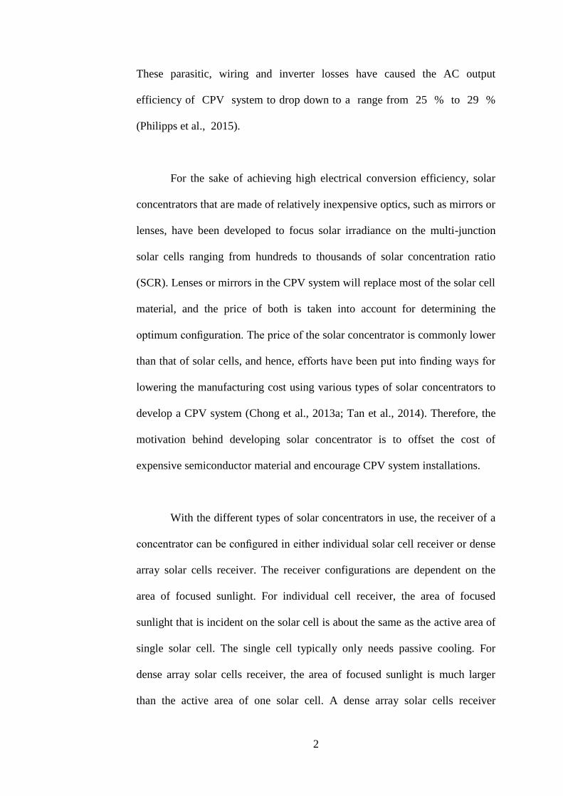
These parasitic, wiring and inverter losses have caused the AC output

efficiency of CPV system to drop down to a range from 25 % to 29 %

(Philipps et al., 2015).

For the sake of achieving high electrical conversion efficiency, solar

concentrators that are made of relatively inexpensive optics, such as mirrors or

lenses, have been developed to focus solar irradiance on the multi-junction

solar cells ranging from hundreds to thousands of solar concentration ratio

(SCR). Lenses or mirrors in the CPV system will replace most of the solar cell

material, and the price of both is taken into account for determining the

optimum configuration. The price of the solar concentrator is commonly lower

than that of solar cells, and hence, efforts have been put into finding ways for

lowering the manufacturing cost using various types of solar concentrators to

develop a CPV system (Chong et al., 2013a; Tan et al., 2014). Therefore, the

motivation behind developing solar concentrator is to offset the cost of

expensive semiconductor material and encourage CPV system installations.

With the different types of solar concentrators in use, the receiver of a

concentrator can be configured in either individual solar cell receiver or dense

array solar cells receiver. The receiver configurations are dependent on the

area of focused sunlight. For individual cell receiver, the area of focused

sunlight that is incident on the solar cell is about the same as the active area of

single solar cell. The single cell typically only needs passive cooling. For

dense array solar cells receiver, the area of focused sunlight is much larger

than the active area of one solar cell. A dense array solar cells receiver

3

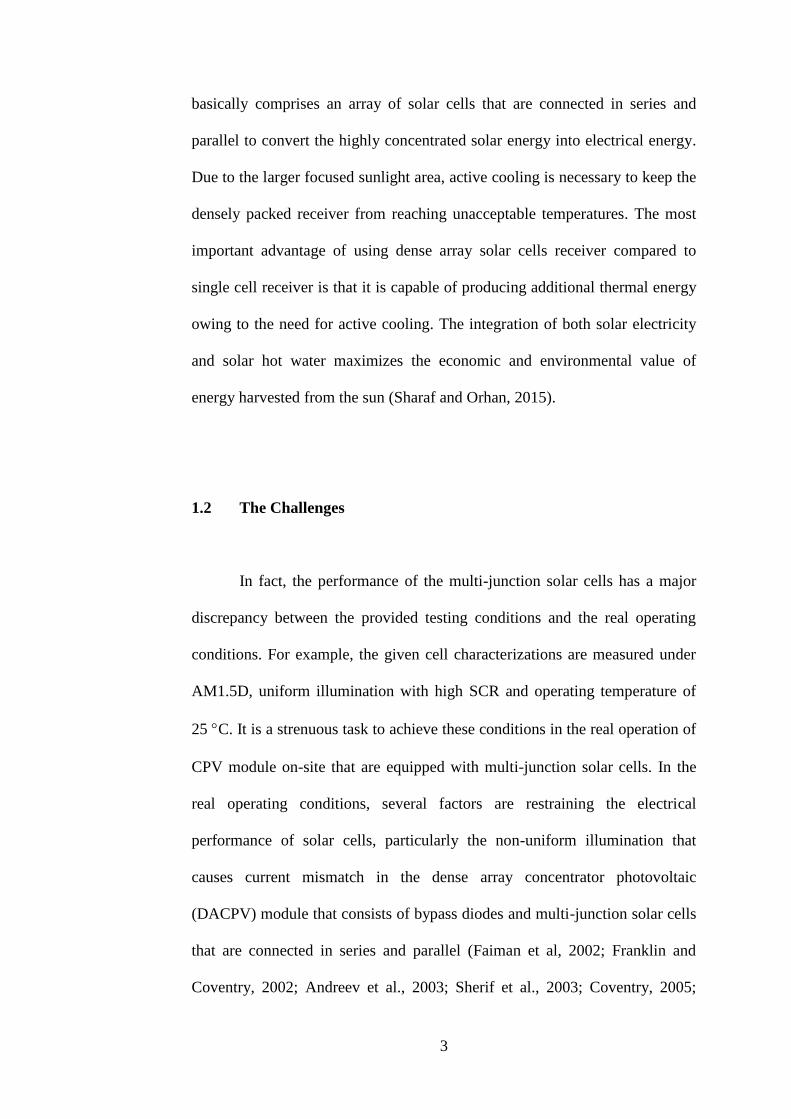
basically comprises an array of solar cells that are connected in series and

parallel to convert the highly concentrated solar energy into electrical energy.

Due to the larger focused sunlight area, active cooling is necessary to keep the

densely packed receiver from reaching unacceptable temperatures. The most

important advantage of using dense array solar cells receiver compared to

single cell receiver is that it is capable of producing additional thermal energy

owing to the need for active cooling. The integration of both solar electricity

and solar hot water maximizes the economic and environmental value of

energy harvested from the sun (Sharaf and Orhan, 2015).

1.2 The Challenges

In fact, the performance of the multi-junction solar cells has a major

discrepancy between the provided testing conditions and the real operating

conditions. For example, the given cell characterizations are measured under

AM1.5D, uniform illumination with high SCR and operating temperature of

25 C. It is a strenuous task to achieve these conditions in the real operation of

CPV module on-site that are equipped with multi-junction solar cells. In the

real operating conditions, several factors are restraining the electrical

performance of solar cells, particularly the non-uniform illumination that

causes current mismatch in the dense array concentrator photovoltaic

(DACPV) module that consists of bypass diodes and multi-junction solar cells

that are connected in series and parallel (Faiman et al, 2002; Franklin and

Coventry, 2002; Andreev et al., 2003; Sherif et al., 2003; Coventry, 2005;

4

Nishioka et al., 2006). When non-uniform illumination is focused on the

module, there will be a significant drop in efficiency as compared with the

module that is operated under uniform illumination (Andreev et al., 2003;

Nishioka et al., 2006; Verlinden et al., 2006). The non-uniform illumination

distributed on the solar cells is mainly caused by optical design limitations,

optical misalignment, low tracking accuracy, circumsolar radiation and the

condition of the refractive lens or reflecting mirrors. (Baig et al., 2012).

1.3 Objectives

In order to overcome the above-identified non-uniform illumination

problem, a systematic and comprehensive study on non-imaging dish

concentrator (NIDC) for the application in DACPV system has been

developed and explored. The main objectives are as follows:

1. To design and construct a prototype of the non-imaging dish

concentrator for the application in dense array concentrator

photovoltaic system.

2. To study the optical characteristics of the non-imaging dish

concentrator with the use of ray-tracing numerical simulation

technique by considering circumsolar radiation, mirror surface slope

error and optical misalignment.

5

3. To develop a systematic method for optimizing the electrical

interconnection of solar cells in dense array concentrator photovoltaic

module configuration to achieve the maximum output power.

4. To design and construct a high concentrated solar flux scanner for

measuring the solar flux distribution of the non-imaging dish

concentrator prototype to validate the numerical simulation results.

1.4 Contributions

The design and construction of cost effective NIDC have been

presented in this study. Instead of using a single piece of the costly parabolic

dish, the NIDC comprises multi-faceted flat mirrors act as an optical aperture

to collect and to focus the incident sunlight at the target with any focal

distance along the optical axis. All the flat facet mirrors are used to

superimpose the sunlight at the receiver, which can produce a reasonably high

SCR and much more uniform solar illumination distributed on the solar cells.

The optical losses of NIDC are less as compared to Fresnel lens system.

Besides, a systematic computational algorithm to study the effects of

imperfection factors, i.e. circumsolar radiation, mirror surface slope error and

optical misalignment, to the solar flux distribution of NIDC has been

developed by using numerical simulation method. A comprehensive analysis

of solar flux distribution at the target has been carried out by considering all

the important criteria to improve the overall performance of DACPV system,

6

such as the maximum SCR, uniform illumination area, and spillage loss. With

the simulated solar flux distribution, the receiver size can be optimized by

minimizing the spillage loss of the DACPV system.

Despite the employment of flat facet mirrors in the NIDC, the resultant

flux distribution from simple super-positioning of all the reflected sunlight is

inevitably non-uniform near the peripheral area. Instead of using non-

conventional solar cells, which incur extra cost and complexity, a systematic

methodology to optimize the layout configuration of solar cells

interconnection circuit in DACPV module has been proposed by minimizing

the current mismatch caused by non-uniformity of concentrated sunlight.

A concentrated solar flux scanner equipped with an array of triple-

junction solar cells has been constructed to measure the solar irradiance across

a receiver plane of NIDC prototype. The flux scanner can perform real time

and direct measurement of high concentrated solar flux distribution profile

with a good degree of accuracy and fast scanning speed. The measured solar

flux profile can be used to validate the numerical simulation that is specially

designed for modeling the solar flux distribution and optimizing the electrical

interconnection of DACPV module. Furthermore, the advantage of this

technique is that the triple-junction solar cells as transducer mounted on the

scanner is the same type as that of assembled in the DACPV module. It has

simplified post-processing layout design of the solar cell interconnection

circuit in the DACPV module because the short-circuit currents of solar cells

7

in their particular locations on the receiver have been measured directly via the

scanner.

1.5 Outline of the Thesis

The organization of the thesis is outlined as follows:

Chapter 1 of this thesis gives an introduction to the research

background and motivation in developing CPV systems. This section

also identifies the challenges in the development of CPV system.

Besides, the project objectives and contributions are clarified in this

chapter.

At first, Chapter 2 gives an introduction to the effects of non-uniform

illumination in CPV System. Next, a literature review about the

various types of solar concentrators and the alternative techniques of

overcoming inhomogeneous illumination in CPV system are presented.

In addition, the techniques to measure solar flux distribution, which

can be classified as direct and indirect measurement methods, are

reviewed.

In Chapter 3, the design and development methodology of NIDC are

discussed in detail including the setup of NIDC prototype and the

design of sun-tracking system.

8

In Chapter 4, the numerical simulation using ray-tracing technique is

presented for the modeling of solar flux distribution on the receiver of

NIDC prototype. The modeling is carried out by considering various

imperfection factors, i.e. circumsolar ratio, mirror surface slope error

and optical misalignment. The simulated solar flux distribution results

are also analyzed in detail.

At the beginning of Chapter 5, the principle of optimizing the circuit

layout of solar cells interconnection is discussed in detail including the

modeling of DACPV module. The electrical performance of the

optimized layout of interconnection solar cells circuit is also discussed

in this chapter.

In Chapter 6, the hardware and software designs of the high

concentrated solar flux scanner are explained in detail. The measured

solar flux profile is also compared with the modeled solar flux profile.

Chapter 7 ends the thesis with the conclusions and future works. The

thesis concludes with the outcomes of the overall research

achievements and the advantages of the developed system.

9

1.6 Publications

Based on the findings from this research, several papers have been

published in peer-reviewed journals and international conference proceedings.

A full list of publications is presented in Table 1.1.

Table 1.1: Papers that are published in peer-reviewed journals and

international conference proceedings.

No

.

Paper Title Year Journal/

Conference

Impart

Factor

1 “Analytical Model of Non-Imaging

Planar Concentrator for the

Application in Dense-Array

Concentrator Photovoltaic System”

(Presented and Published)

2013

1st International

Symposium on

Innovative

Technologies for

Engineering and

Science

N/A

2 "Flux Distribution Analysis of Non-

Imaging Planar Concentrator

Considering Effects of Circumsolar

Radiation and Mirror Slope Error"

(Presented and Published)

2014

Light Energy and

the Environment

Congress

N/A

3 “Performance Optimization of

Dense-Array Concentrator

Photovoltaic System Considering

Effects of Circumsolar Radiation and

Slope Error”

(Published)

2015 Optics Express 3.488

4 “Solar Flux Distribution Study of

Non-Imaging Dish Concentrator

Using Linear Array of Triple-

Junction Solar Cells Scanning

Technique”

(Published)

2016 Solar Energy 3.469

10

CHAPTER 2

LITERATURE REVIEW

2.1 Introduction

To further reduce the cost of CPV power generation systems, optimal

system design is necessary so that maximum solar energy can be harnessed

from the solar cells (Luque et al., 2006; Nishioka et al., 2006). However, we

often find that the delivered electrical power in field conditions is much lower

than the array ratings because mismatch losses have affected the current-

voltage (I-V) and power-voltage (P-V) curves of the solar cells. Mismatch

factors such as soiling, non-uniform irradiance, shading, temperature

variations, cell’s quality as well as aging of solar cells, all contribute to serious

array power reduction in real site testing (Kaushika and Rai; 2007; Picault e al.,

2010; Baig et al., 2012).

2.2 Effects of Non-Uniform Illumination in CPV System

Non-uniform distribution of concentrated solar irradiance is one of the

most significant problems faced by most of CPV systems, especially around

the receiver edges, mainly caused by optical design limitations, structure

misalignment, and low tracking accuracy (Baig et al., 2012). Over the recent

11

years, many studies can be found discussing on the improvement of solar

concentrator optical design to produce more uniform solar illumination at high

concentrations (Chong et al., 2013a). Nevertheless, the overall output current

of multi-junction cells connected in a dense array arrangement is very much

dependent on the solar flux distribution of a solar concentrator. Due to factors

such as sun-shape, circumsolar effect, aberration, imperfection of mirror’s

geometry, etc., it is impossible to produce perfect uniform illumination on the

dense array concentrator photovoltaic (DACPV) receiver and hence causing a

significant loss in the overall output power and average conversion efficiency

(Faiman et al, 2002; Franklin and Coventry, 2002; Andreev et al., 2003; Sherif

et al., 2003; Coventry, 2005; Nishioka et al., 2006).

In recent years, researchers have presented several approaches to study

the effects of non-uniform illumination on the performance of solar cells. For

example, Reis et al. (2013) introduced a distributed diode model for solar cells

to predict the behavior of solar cells that are integrated into CPV systems. The

modeling showed that there is a power loss when solar cells operate under

conditions of inhomogeneous distribution of temperature and illumination.

Furthermore, Cooper et al. (2013) have experimentally validated a model with

a linear semi-dense array of five series-connected triple-junction concentrator

cells. Under the worst-case conditions of non-uniform illumination on the

array, the efficiency of the array drops to 28.5% as compared to 39% for the

case of perfect uniformity.

12

2.3 Optical Design of Solar Concentrators

Solar concentrator plays a vital role in the research and development of

CPV power generation system. The solar concentrator makes use of

geometrical optics in the design of reflective or refractive types of

concentrating devices to focus the solar flux onto a receiver module equipped

with multi-junction solar cells (Chong et al., 2013b). Generally, solar

concentrators can be categorized into two major groups: imaging concentrator

and non-imaging concentrator (Winston et al., 2005; Heinloth, 2006; Luque

and Andreev, 2007). Despite being widely used in optics applications such as

astronomical telescope and camera, the imaging concentrator does not aim to

produce uniform flux distribution profile at the receiver that is highly required

in the DACPV module (Chong et al., 2010). The DACPV module that

receives non-uniform solar illumination will face a severe drop in efficiency

due to the current mismatch problem as opposed to the module under uniform

solar illumination (Andreev et al., 2003; Nishioka et al., 2006; Verlinden et al.,

2006).

How to form a uniform solar illumination on the solar cells is a great

challenge for the researchers who are working in CPV power generation

system. In recent years, several researchers have paid a lot of efforts to design

various types of solar concentrators for producing a uniform distribution of

solar radiation on the solar cells.

13

2.3.1 Parabolic Dish Concentrator

Over the last few decades, a parabolic dish concentrator has been

widely used for solar energy applications, especially for applications involving

high solar concentration and high-temperature collection. For a large dish

concentrator system, using a single parabolic mirror as a reflector is costly due

to the special technology needed to fabricate special mirrors with a thickness

from 0.7 to 1.0 mm and to obtain the parabolic shape (Kussul et al., 2008). For

a large collective area of parabolic dish concentrator, multi-faceted spherical

or concave mirrors are arranged on the approximate parabolic shape structure

as a reflector instead of using a single piece of the parabolic reflector

(Johnston et al., 2003; Ulmer et al., 2008). Despite alignment of mirrors being

required in a faceted parabolic concentrator, its fabrication is cheaper and

simpler as compared with a single precise parabolic reflector.

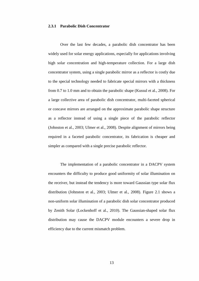
The implementation of a parabolic concentrator in a DACPV system

encounters the difficulty to produce good uniformity of solar illumination on

the receiver, but instead the tendency is more toward Gaussian type solar flux

distribution (Johnston et al., 2003; Ulmer et al., 2008). Figure 2.1 shows a

non-uniform solar illumination of a parabolic dish solar concentrator produced

by Zenith Solar (Lockenhoff et al., 2010). The Gaussian-shaped solar flux

distribution may cause the DACPV module encounters a severe drop in

efficiency due to the current mismatch problem.

14

Figure 2.1: Non-uniform solar illumination of a parabolic dish solar

concentrator (Lockenhoff et al., 2010).

In order to solve the current mismatch problem, two-stage solar

concentrators that comprise a parabolic dish and secondary optics or

homogenizer have been introduced for the application of a CPV system

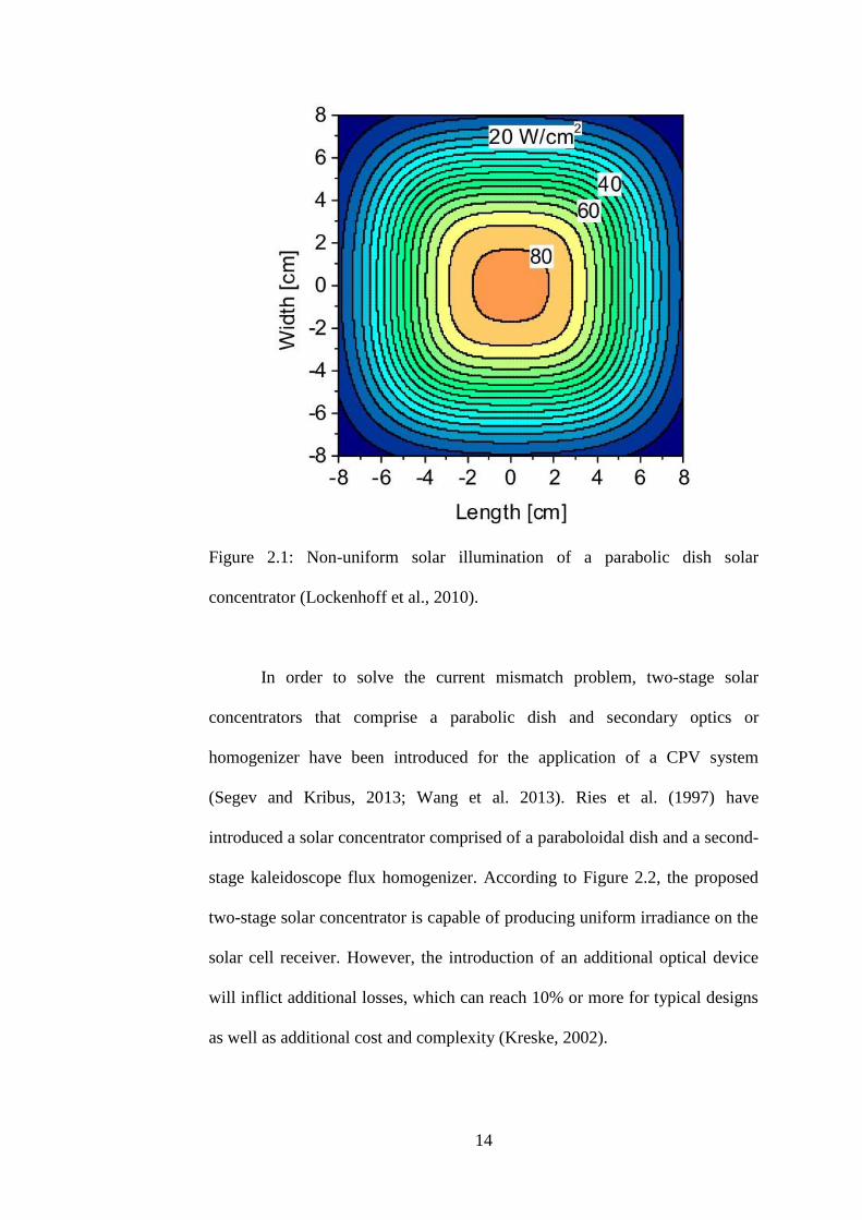
(Segev and Kribus, 2013; Wang et al. 2013). Ries et al. (1997) have

introduced a solar concentrator comprised of a paraboloidal dish and a second-

stage kaleidoscope flux homogenizer. According to Figure 2.2, the proposed

two-stage solar concentrator is capable of producing uniform irradiance on the

solar cell receiver. However, the introduction of an additional optical device

will inflict additional losses, which can reach 10% or more for typical designs

as well as additional cost and complexity (Kreske, 2002).

15

Figure 2.2: A comparison of irradiance distribution using paraboloidal-dish

only and paraboloidal-dish plus kaleidoscope flux homogenizer (Ries et al.,

1997).

2.3.2 Fresnel Concentrator

Besides the aforementioned parabolic dish concentrators, researchers

have proposed various kinds of Fresnel concentrators for the sake of

producing uniform solar flux distribution on the solar cells, which can be

classified as Fresnel reflector and Fresnel lens (Chong et al., 2013). Mills and

Morrison (2002) advocated the use of an advanced form of compact linear

Fresnel reflector (CLFR) that can produce a better uniformity of solar

irradiation compared to parabolic trough or parabolic dish systems. However,

the SCR for linear Fresnel reflector is normally lower than 100 suns (Chong et

al., 2010; Tan et al., 2014).

16

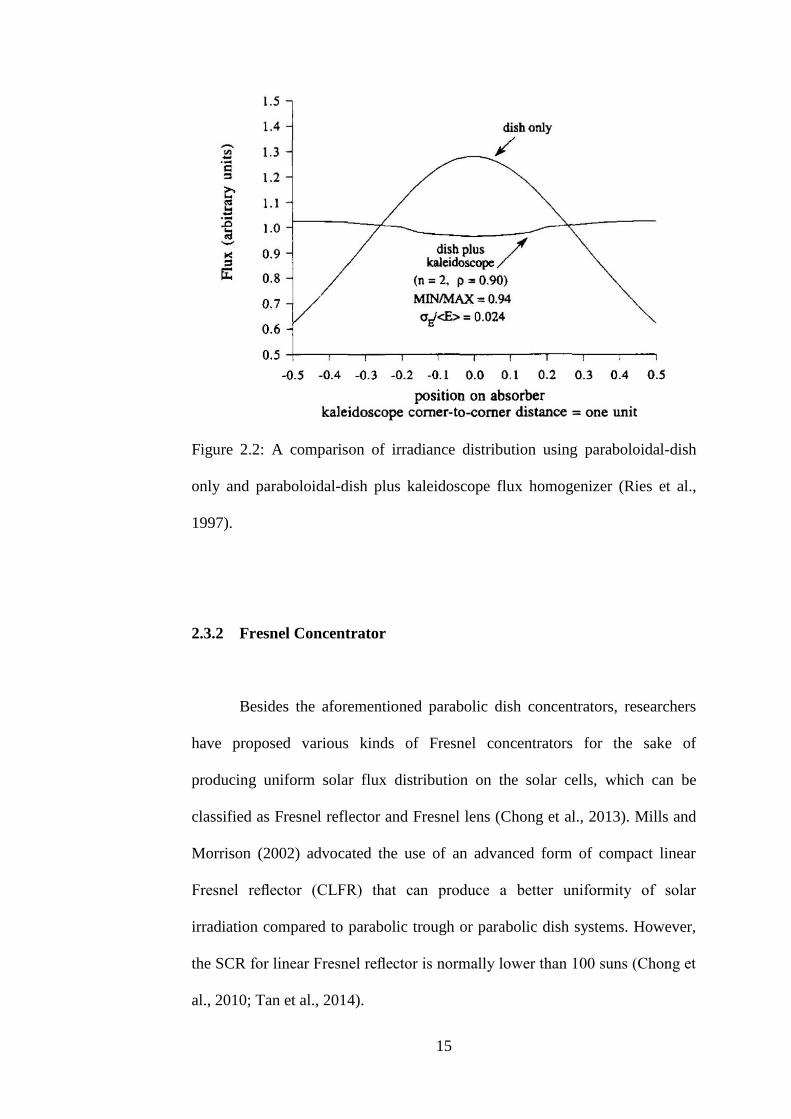
In Fresnel lens system, an additional secondary optical element (SOE)

such as flux homogenizer is needed to produce uniform solar flux distribution,

since the conventional Fresnel lenses always focus a collimated beam to a

point, as presented in Figure 2.3 (Ota and Nishioka, 2012). This approach is

capable of cutting down the expensive solar cell area by increasing the SCR

and the light intensity. However, there are some other factors causing the

inhomogeneous illumination distributed on the solar cells, such as tracking

error, misalignment of the concentrator and the condition of the refractive lens

or reflecting mirrors (Baig et al., 2012; Chong et al., 2013).

Figure 2.3: A comparison of simulated irradiance distribution on the solar cell

using Fresnel lens only and Fresnel lens plus homogenizer (Ota and Nishioka,

2012).

Ryu et al. (2006) introduced a modular Fresnel concentrator for

achieving moderate SCR (several hundreds of suns) and better uniform solar

illumination on the solar cell. Figure 2.4 shows the superposition concept of

modular Fresnel lenses for CPV system. Each modular Fresnel lens refracts

the incident sunlight onto the targeted solar cell. Conversely, the transmission

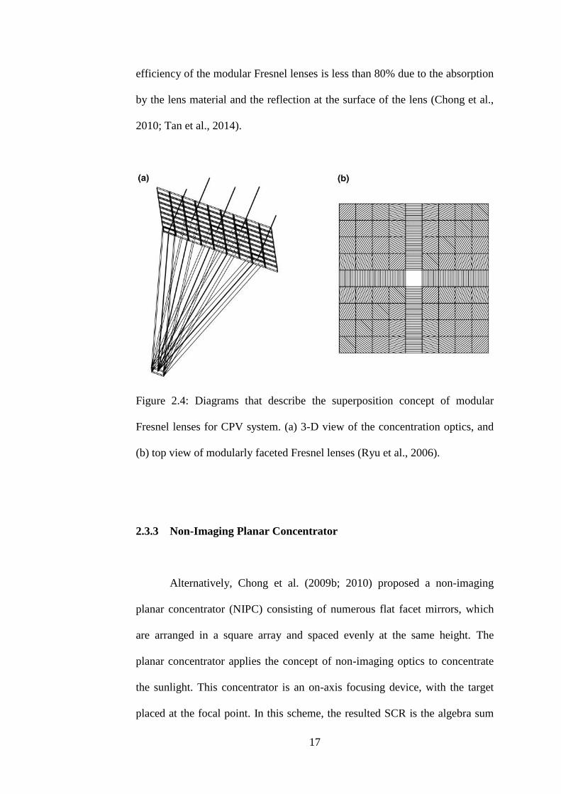
17

efficiency of the modular Fresnel lenses is less than 80% due to the absorption

by the lens material and the reflection at the surface of the lens (Chong et al.,

2010; Tan et al., 2014).

Figure 2.4: Diagrams that describe the superposition concept of modular

Fresnel lenses for CPV system. (a) 3-D view of the concentration optics, and

(b) top view of modularly faceted Fresnel lenses (Ryu et al., 2006).

2.3.3 Non-Imaging Planar Concentrator

Alternatively, Chong et al. (2009b; 2010) proposed a non-imaging

planar concentrator (NIPC) consisting of numerous flat facet mirrors, which

are arranged in a square array and spaced evenly at the same height. The

planar concentrator applies the concept of non-imaging optics to concentrate

the sunlight. This concentrator is an on-axis focusing device, with the target

placed at the focal point. In this scheme, the resulted SCR is the algebra sum

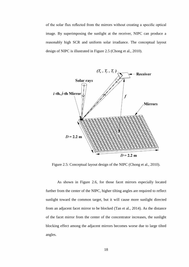
18

of the solar flux reflected from the mirrors without creating a specific optical

image. By superimposing the sunlight at the receiver, NIPC can produce a

reasonably high SCR and uniform solar irradiance. The conceptual layout

design of NIPC is illustrated in Figure 2.5 (Chong et al., 2010).

Figure 2.5: Conceptual layout design of the NIPC (Chong et al., 2010).

As shown in Figure 2.6, for those facet mirrors especially located

further from the center of the NIPC, higher tilting angles are required to reflect

sunlight toward the common target, but it will cause more sunlight directed

from an adjacent facet mirror to be blocked (Tan et al., 2014). As the distance

of the facet mirror from the center of the concentrator increases, the sunlight

blocking effect among the adjacent mirrors becomes worse due to large tilted

angles.

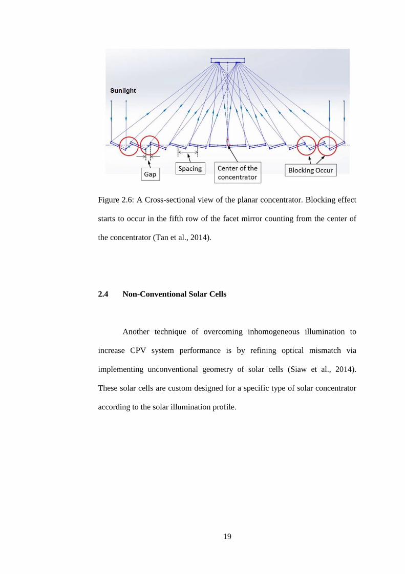
19

Figure 2.6: A Cross-sectional view of the planar concentrator. Blocking effect

starts to occur in the fifth row of the facet mirror counting from the center of

the concentrator (Tan et al., 2014).

2.4 Non-Conventional Solar Cells

Another technique of overcoming inhomogeneous illumination to

increase CPV system performance is by refining optical mismatch via

implementing unconventional geometry of solar cells (Siaw et al., 2014).

These solar cells are custom designed for a specific type of solar concentrator

according to the solar illumination profile.

20

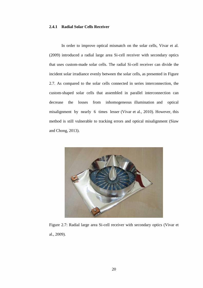
2.4.1 Radial Solar Cells Receiver

In order to improve optical mismatch on the solar cells, Vivar et al.

(2009) introduced a radial large area Si-cell receiver with secondary optics

that uses custom-made solar cells. The radial Si-cell receiver can divide the

incident solar irradiance evenly between the solar cells, as presented in Figure

2.7. As compared to the solar cells connected in series interconnection, the

custom-shaped solar cells that assembled in parallel interconnection can

decrease the losses from inhomogeneous illumination and optical

misalignment by nearly 6 times lesser (Vivar et al., 2010). However, this

method is still vulnerable to tracking errors and optical misalignment (Siaw

and Chong, 2013).

Figure 2.7: Radial large area Si-cell receiver with secondary optics (Vivar et

al., 2009).

21

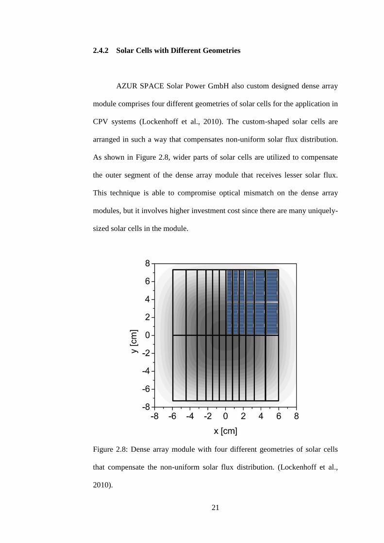
2.4.2 Solar Cells with Different Geometries

AZUR SPACE Solar Power GmbH also custom designed dense array

module comprises four different geometries of solar cells for the application in

CPV systems (Lockenhoff et al., 2010). The custom-shaped solar cells are

arranged in such a way that compensates non-uniform solar flux distribution.

As shown in Figure 2.8, wider parts of solar cells are utilized to compensate

the outer segment of the dense array module that receives lesser solar flux.

This technique is able to compromise optical mismatch on the dense array

modules, but it involves higher investment cost since there are many uniquely-

sized solar cells in the module.

Figure 2.8: Dense array module with four different geometries of solar cells

that compensate the non-uniform solar flux distribution. (Lockenhoff et al.,

2010).

22

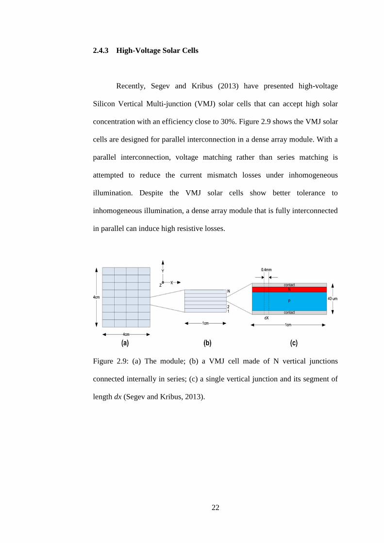
2.4.3 High-Voltage Solar Cells

Recently, Segev and Kribus (2013) have presented high-voltage

Silicon Vertical Multi-junction (VMJ) solar cells that can accept high solar

concentration with an efficiency close to 30%. Figure 2.9 shows the VMJ solar

cells are designed for parallel interconnection in a dense array module. With a

parallel interconnection, voltage matching rather than series matching is

attempted to reduce the current mismatch losses under inhomogeneous

illumination. Despite the VMJ solar cells show better tolerance to

inhomogeneous illumination, a dense array module that is fully interconnected

in parallel can induce high resistive losses.

Figure 2.9: (a) The module; (b) a VMJ cell made of N vertical junctions

connected internally in series; (c) a single vertical junction and its segment of

length dx (Segev and Kribus, 2013).

23

2.5 Techniques to Measure Solar Flux Distribution

The major challenge for achieving high performance of DACPV

module is the non-uniform illumination that results in the current mismatch

among the cells connected in series. For that reason, an accurate measurement

is necessary to obtain the high SCR profile for each location of the solar cell

on the receiver of the solar concentrator. The high SCR profile can be used to

validate the numerical simulation that is specially designed for modeling the

solar flux distribution and optimizing the electrical interconnection of DACPV

module.

How to measure high concentrated solar flux distribution accurately is

an onerous challenge for the researchers who are working in solar facilities. In

recent years, several research laboratories have paid great efforts to design

various types of instruments for measuring the high concentration solar flux

distribution, which can be classified as direct and indirect measurement

methods (Röger et al., 2014).

2.5.1 Direct Measurement Method

In the direct measurement method, Gardon type calorimeter, also

known as a thermo gauge, is the most commonly used heat flux sensor that

directly delivers a measurement signal proportional to the solar flux. Estrada et

al. (2007) developed a calorimeter with the utilization of the cold water

24

calorimetry technique for measuring the concentrated solar flux produced by a

point focus solar concentrator. The solar flux was measured via determining

the heat absorbed by a cooling fluid circulated through the calorimeter (see

Figure 2.10). To estimate the concentrated solar flux, a balance between the

energy absorbed by the fluid and the solar energy focuses on the calorimeter

was carried out. In overall, calorimeter is employed to measure thermal

radiation, and a series of special calibration to the solar radiation spectrum is

carried out with the heat radiation from a blackbody at 850°C (Ballestrín et al.,

2003; Ballestrín et al., 2004; Parretta et al., 2007; Fernandez-Reche et al.,

2008).

Figure 2.10: (a) A picture of the flat plate calorimeter and (b) cross-sectional

diagram to show how the solar flux was measured via determining the heat

absorbed by a cooling fluid circulated through the calorimeter (Estrada et al.,

2007).

25

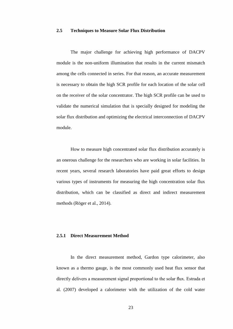
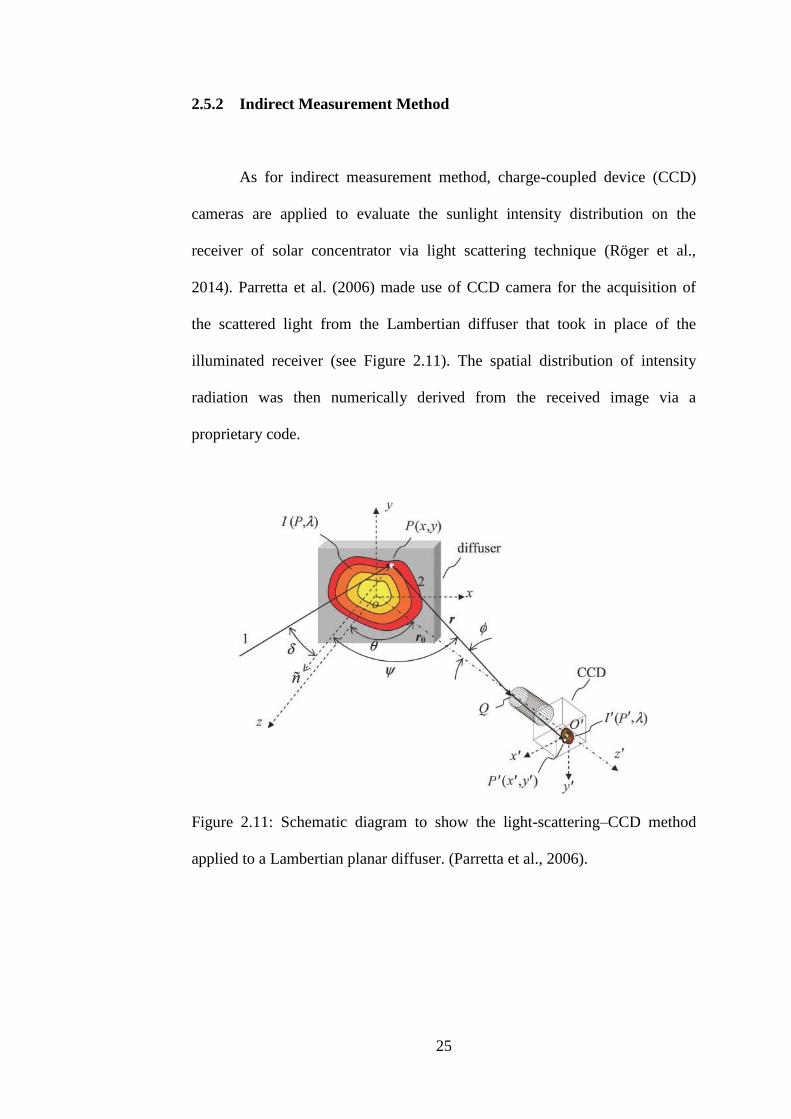
2.5.2 Indirect Measurement Method

As for indirect measurement method, charge-coupled device (CCD)

cameras are applied to evaluate the sunlight intensity distribution on the

receiver of solar concentrator via light scattering technique (Röger et al.,

2014). Parretta et al. (2006) made use of CCD camera for the acquisition of

the scattered light from the Lambertian diffuser that took in place of the

illuminated receiver (see Figure 2.11). The spatial distribution of intensity

radiation was then numerically derived from the received image via a

proprietary code.

Figure 2.11: Schematic diagram to show the light-scattering–CCD method

applied to a Lambertian planar diffuser. (Parretta et al., 2006).

26

Besides, Haueter et al. (1999) and Ulmer et al. (2002) can measure

ultra-high concentrated sunlight up to 5,000 suns and 12,000 suns respectively

by using appropriate combinations of neutral density filters and cooling

devices. Despite the CCD camera having fast response time, flux gauges or

calorimeters were required for the calibration of brightness maps provided by

the CCD cameras (Röger et al., 2014; Salomé et al., 2013).

27

CHAPTER 3

DESIGN AND CONSTRUCTION OF NON-IMAGING DISH

CONCENTRATOR

3.1 Introduction

Inspired by adopting the merit ideas from both NIPC (to produce

reasonably uniform illumination with the use of flat facet mirrors) and

parabolic dish concentrator (to avoid the sunlight blocking and shadowing

effects with the geometry gradually increase in height), the author and his

research teammates have proposed the non-imaging dish concentrator (NIDC)

with single-stage focusing by extracting the best designs from both solar

concentrators (Chong et al, 2012b; Chong et al, 2013b; Tan et al, 2014). The

proposed NIDC is an optical device that is specially designed for the

application in DACPV system, which requires uniform flux distribution on the

receiver.

3.2 Principle of NIDC

To achieve a good uniformity of the solar irradiation with a reasonably

high SCR on the target, a NIDC has been proposed by applying the concept of

non-imaging optics to concentrate the sunlight. The NIDC is formed by

28

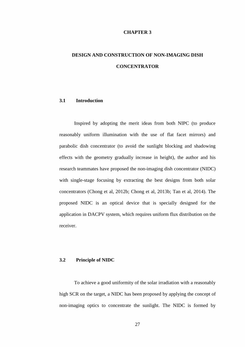
numerous square flat mirrors act as the optical aperture to collect and to focus

the incident sunlight into a target. The conceptual layout design of the NIDC is

illustrated in Figure 3.1. The idea of concentrating the sunlight in the NIDC is

similar to that of NIPC, where the uniform flux distribution on the target can

be acquired from the superposition of the reflected sunlight. In this design, the

incident sunrays are reflected by an array of identical flat mirrors to the target,

in which their size and shape are nearly same as that of the receiver. In order

to eliminate blocking and shadowing effects from the adjacent facet mirrors,

Tan et al. (2014) introduced a computational algorithm to determine the facet

mirrors configuration for the NIDC. The NIDC geometry was designed

according to the proposed algorithm. As shown in Figure 3.1, the facet mirrors

are gradually lifted from central to peripheral regions of the dish concentrator.

Figure 3.1: Conceptual layout design of the NIDC. All the flat facet mirrors

are gradually lifted from central to peripheral regions of the concentrator to

prevent shadowing and blocking among adjacent mirrors.

29

3.3 Prototype of NIDC

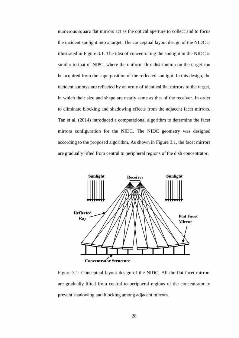
Figure 3.2 shows the prototype of NIDC located in Universiti Tunku

Abdul Rahman (UTAR), Kuala Lumpur campus, Malaysia (3.22 North,

101.73 East). This prototype is capable of producing much more uniform

spatial irradiance for the application in DACPV system. Instead of using a

single piece of the parabolic dish, the NIDC consisting of multi-faceted

mirrors act as the optical aperture to collect and to focus the incident sunlight

at the common receiver that is placed at a focal distance of 210 cm.

Figure 3.2: The prototype of NIDC located in Universiti Tunku Abdul

Rahman (UTAR), Kuala Lumpur campus, Malaysia (3.22 North, 101.73

East).

30

3.3.1 Hardware Design

The structure of the dish concentrator can be divided into two main

components: concentrator frame and flat facet mirror sets. The main material

that is selected for constructing the solar concentrator frame is 20 mm × 20

mm square hollow aluminum bars with a thickness of 1 mm. The hollow bar is

preferred because of weather resistant, significant savings in raw material cost

and light weight compared to the solid bar. Because of that, the concentrator

frame will not apply much load on the turning mechanism, and subsequently,

eases the process of structure development. Sections of the square hollow steel

bars are joined in vertically and horizontally to form the concentrator frame.

Another structure, which is the target supporter, is built by using two sets of

square hollow bars. The target is fixed at a focal point with the distance of 210

cm away from the center of solar concentrator frame.

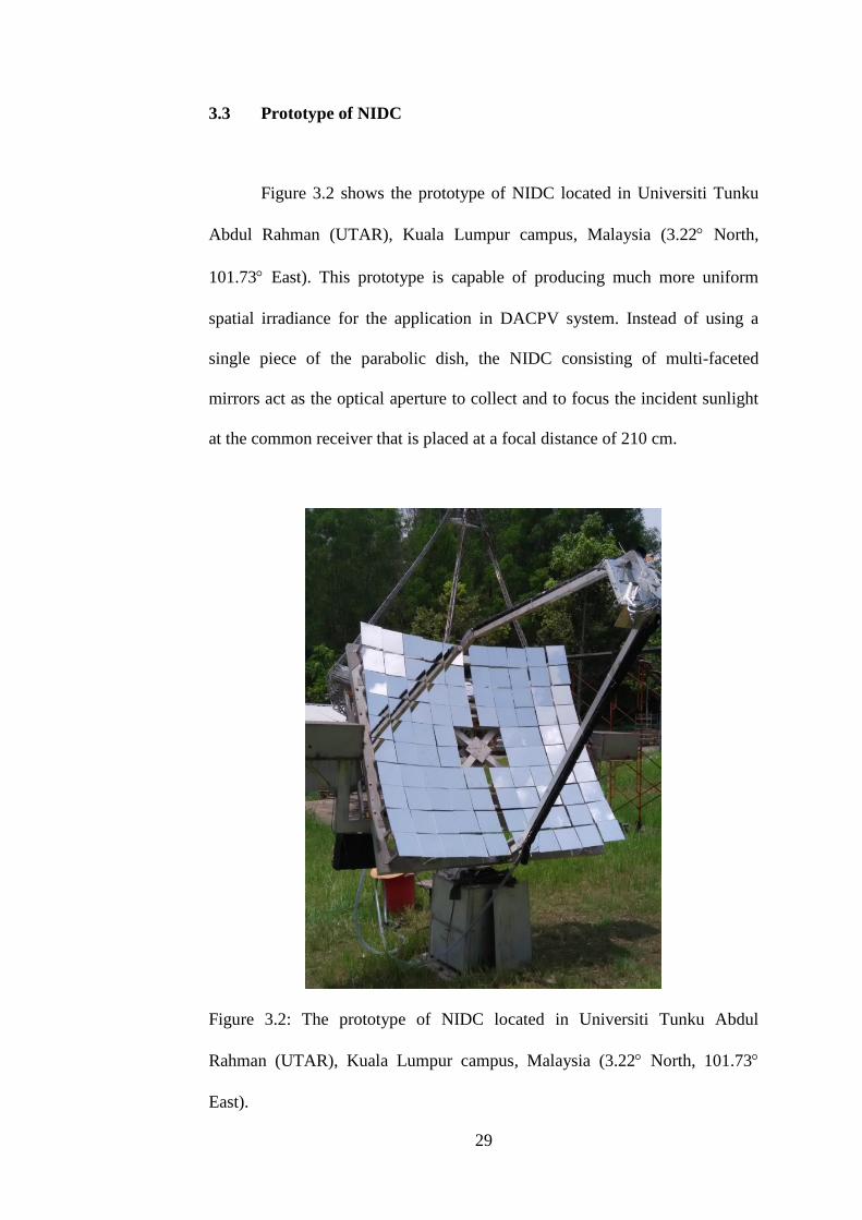
Figure 3.3 shows the prototype consists of 96 flat facet mirror sets to

be arranged into ten rows and ten columns on the concentrator frame. Four

mirror sets in the central region of concentrator are omitted due to the shading

by the receiver. Flat facet mirrors with a dimension of 20 cm × 20 cm and a

thickness of 0.3 cm are selected to form a total reflective area of 3.84 m².

There is a gap spacing of 0.5 cm in between the mirrors. This gap will avoid

any possible blocking when the mirrors are tilted and can also reduce the wind

pressure on the concentrator frame. Besides, the flat facet mirror sets consist

of several other components, namely, the compression springs, machine

screws, silicone pastes and wing nuts (Chong et al., 2009b). The idea of this

31

design is for the presetting of each mirror along the row and column directions.

There are three contact points in each of this screw–spring assembly from

which one of them acts as the pivot point, and the remaining two are

adjustable points. Each mirror can thus be freely tilted to focus sunlight onto

the target by turning the nuts of the adjustable screw–spring sets manually.

Figure 3.3: Schematic diagram shows the arrangements of 96 flat facet mirror

sets with a dimension of 20 cm × 20 cm each that are arranged in ten rows and

ten columns on the prototype in which four mirror sets at the central region of

concentrator are omitted.

32

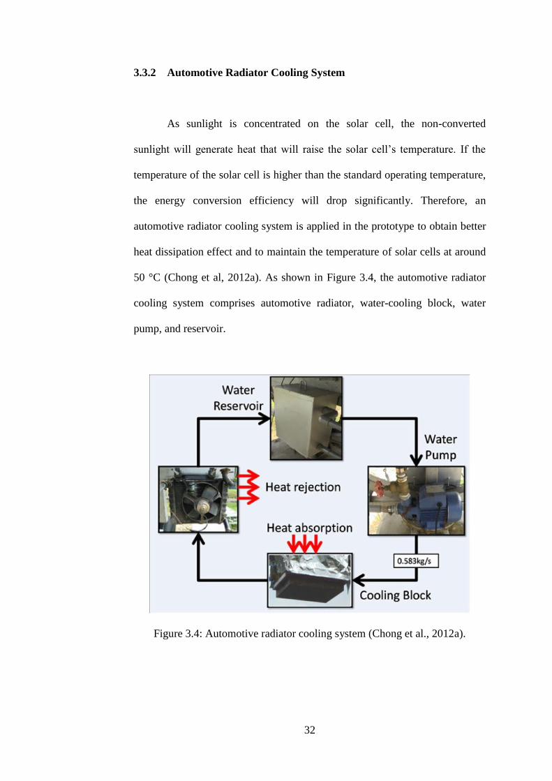
3.3.2 Automotive Radiator Cooling System

As sunlight is concentrated on the solar cell, the non-converted

sunlight will generate heat that will raise the solar cell’s temperature. If the

temperature of the solar cell is higher than the standard operating temperature,

the energy conversion efficiency will drop significantly. Therefore, an

automotive radiator cooling system is applied in the prototype to obtain better

heat dissipation effect and to maintain the temperature of solar cells at around

50 °C (Chong et al, 2012a). As shown in Figure 3.4, the automotive radiator

cooling system comprises automotive radiator, water-cooling block, water

pump, and reservoir.

Figure 3.4: Automotive radiator cooling system (Chong et al., 2012a).

33

An automotive radiator has been used as the key device for the heat

rejection in the cooling system. The materials of automotive radiator casing

and tubes are aluminum alloy with high heat conductivity and light weight. It

is easy to be installed into the prototype of NIDC with minimum load added to

the driving system. The external fins sandwiched between the ducts in the

radiator are made of copper in order to have higher heat conductivity for

increasing heat dissipation rate. The total heat transfer area of radiator is

reasonably large, which includes the surface areas of radiator ducts and of

copper fins.

A copper water-cooling block is selected as a receiver to obtain better

heat dissipation effect and to prevent the solar cell from operating at a high

temperature. In this study, the preferred material of the cooling block is copper

owing to its high thermal conductivity. A DC water pump is utilized for

circulating water between the radiator and the cooling block. Its role is to

create a constant water speed in whole automotive radiator cooling system at

mass flow rate of 0.583 kg/s. Last but not least, the final component is a

reservoir tank which acts as the start point and end point of the water

circulation in the automotive radiator cooling system. It also provides

additional space for storing back flow water when the system stops operation

and to control the total volume of water in the whole cooling system at about

12 liters.

34

3.3.3 Sun-Tracking System

In order to maintain a high output power and stability of the DACPV

system, a high-precision of the sun-tracking system is required to follow the

sun’s trajectory throughout the day. This prototype is designed to operate on

the most common two-axis sun tracking system, which is azimuth-elevation

sun-tracking system.

The drive mechanism for the solar concentrator consists of stepper

motors and associated gears. Two stepper motors, with the specification of

0.05 degree in full step, are coupled to the elevation and azimuth shafts

respectively for driving the concentrator to its desired position. Each stepper

motor is coupled to its respective shaft via a worm gearbox with a gear ratio of

60:1, yielding an overall resolution of 8.33 × 10– 4 /step. Compared with

ordinary gear trains using spur gears, the direction of worm gear transmission

is irreversible because a larger friction involved between the worm and worm-

wheel. In other words, worm gear configurations in which the gear cannot

drive the worm are said to be self-locking. In this way, there is no motor

energy consumption on stationary positions and the usage of complex load

brake mechanisms is not required.

An open-loop control system is preferable for the prototype of solar

concentrator so as to keep the design of the sun-tracking system simple and

cost effective. Open-loop sensors, two 12-bit absolute optical encoders are

attached to the shafts of the azimuth and elevation axes of the concentrator

35

respectively to monitor the turning angles and to send feedback signals to the

controller if there is any abrupt change in the encoder reading. The sensors not

only ensure that the instantaneous azimuth and elevation angles are matched

with the calculated values from the controller but also eliminate any tracking

errors due to the mechanical backlash, accumulated error, wind effects and

other disturbances to the solar concentrator. With the optical encoders, any

discrepancy between the calculated angles and real-time angles of solar

concentrator can be detected, whereby the drive mechanism will be activated

to move the solar concentrator to the correct position.

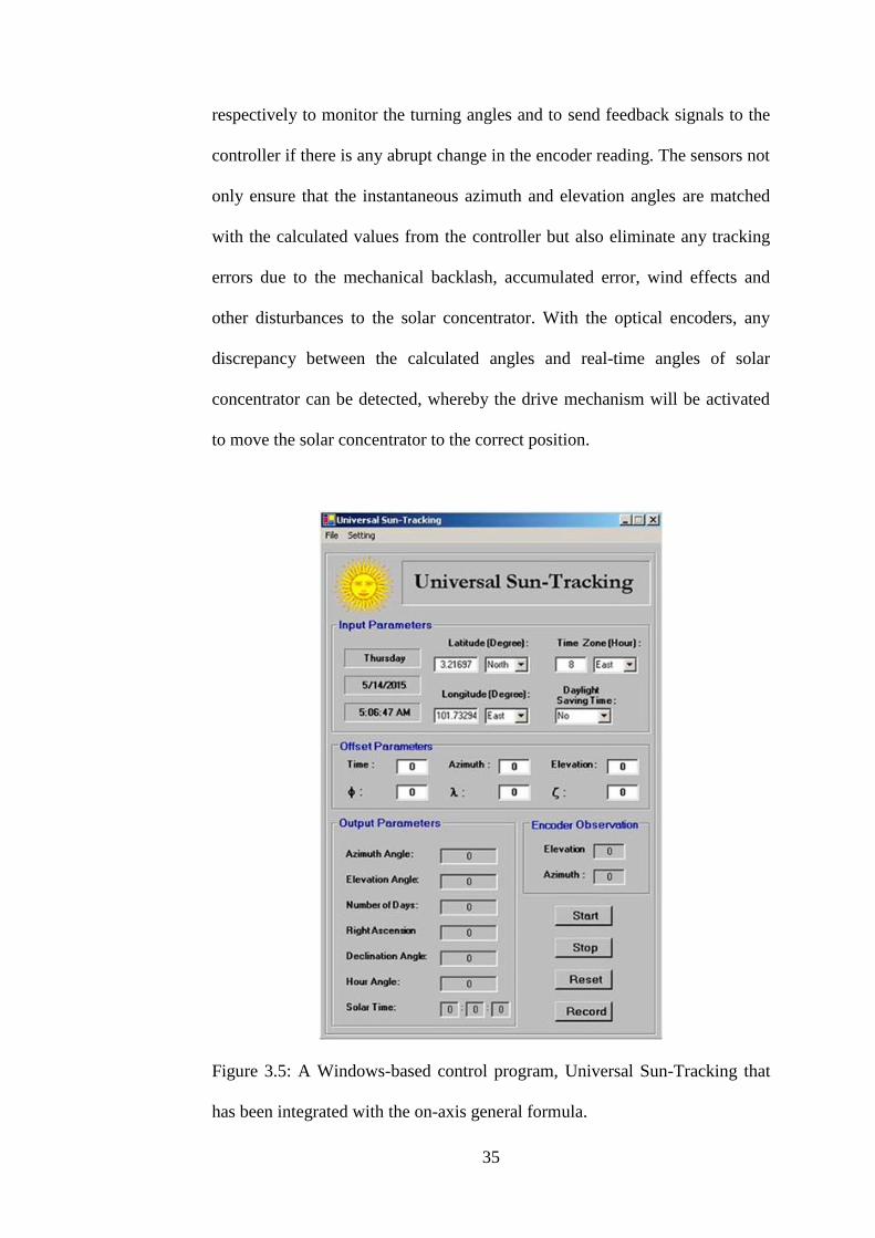
Figure 3.5: A Windows-based control program, Universal Sun-Tracking that

has been integrated with the on-axis general formula.

36

A Windows-based control program was developed by integrating the

general sun-tracking formula to control the sun-tracking mechanism along the

azimuth and elevation axes (see Figure 3.5). The merit of the general sun-

tracking formula is that it can simplify the fabrication and installation work of

solar concentrator with higher tolerance in terms of the tracking axes

alignment (Chong and Wong 2009; Chong et al., 2009a; Chong and Wong,

2010).

In the control algorithm, the sun-tracking angles (azimuth and

elevation) are first computed according to the given information, i.e. local

clock time, date, geographical location, time zone, daylight saving time and

three misalign angles. The control program then generates digital pulses that

are sent to the stepper motor driver via parallel port to drive the solar

concentrator to the pre-calculated angles along azimuth and elevation

movements in sequence. Each time, the control program only activates one of

the two stepper motors through a relay switch. The tracker is programmed to

follow the sun at all times since the program is run in repeated loops (every 1

minute). A feedback signal is sent when the difference between the calculated

angles and encoders’ reading is larger than the encoder resolution, which is

0.176. Figure 3.6 shows the block diagram of the open-loop sun-tracking

system implemented in this prototype.

37

Figure 3.6: Block diagram to show the complete open-loop sun-tracking

system of the NIDC.

3.4. Mirror Alignment

Based on the principle of NIDC, mirror alignment is essential to

produce a uniform solar flux distribution through the superposition of all the

reflected sunlight on the receiver. There are two stages in the mirror alignment

process. The first stage is to fine tune the input parameters for the sun-tracking

system so that the solar concentrator can track the sun accurately. The

parameters that will affect the tracking accuracy are latitude, longitude, local

clock time and the misalign angles. At this stage, four mirrors which are close

to the center of the concentrator frame are selected to concentrate sunlight

onto the target during the sun-tracking, whereas the remaining mirrors are

covered. When the exposed mirrors achieve the smallest tracking error, a

small offset value from the reflected sunlight to the expected target area, the

second stage of mirror alignment can be started. The second stage is to tilt the

remaining mirrors to focus sunlight towards the target. This mirror alignment

38

work must be carried out while the concentrator mirrors are in operation and

tracking the sun.

3.5 Summary

A new configuration of solar concentrator, which is the non-imaging

dish concentrator, has been designed and constructed. This prototype is

capable of producing reasonably uniform solar flux distribution and high SCR

for the application in DACPV system. Instead of using a single piece of

parabolic dish, the NIDC consisting of 96 flat facet mirrors with a dimension

of 20 cm × 20 cm act as the optical aperture. Each facet mirror has been tilted

to collect and to reflect the incident sunlight onto the common receiver that is

placed at a focal distance of 210 cm. Besides, the automotive radiator cooling

system is applied in the prototype for the heat management purpose to lower

down the temperature of solar cells. The prototype is orientated to face the

direct sunlight by using the most common two-axis sun-tracking system,

which is azimuth-elevation tracking system.

39

CHAPTER 4


CONCENTRATOR

4.1 Introduction

The NIDC comprised of multi-faceted mirrors act as an optical

aperture to collect and focus the incident sunlight at any focal distance along

the optical axis. Different from imaging optical devices such as parabolic

reflectors, the geometry of NIDC cannot be explicitly defined by any

analytical surface formula, and thus, numerical simulation is a necessary

means in optical analysis. For the optical modeling of the NIDC, the author

has employed coordinate transformations and ray-tracing technique to express

the reflection of sunlight by the dish concentrator as well as to generate the

solar flux distribution on the receiver plane (Wong et al., 2015).

4.2 Optical Characterization

A numerical simulation using ray-tracing method has been developed

for modeling the solar flux distribution profile on the receiver of NIDC

prototype by assuming unity mirror reflectivity. In reflection-based solar

concentrators, reflected rays could deviate from the specular reflection

40

direction and eventually not hitting on the receiver mainly caused by

circumsolar radiation, mirror surface slope error and optical misalignment.

This small angular deviation of sunray may bring a significant effect to the

solar flux distribution at the receiver. As a result, the modeling of solar flux

distribution is carried out by considering various imperfection factors, i.e.

circumsolar ratio, mirror surface slope error and optical misalignment (Wong

et al., 2015). The imperfection factors mentioned above are never discussed in

the design and development of NIPC, which proposed by Chong et al. (2009b;

2010).

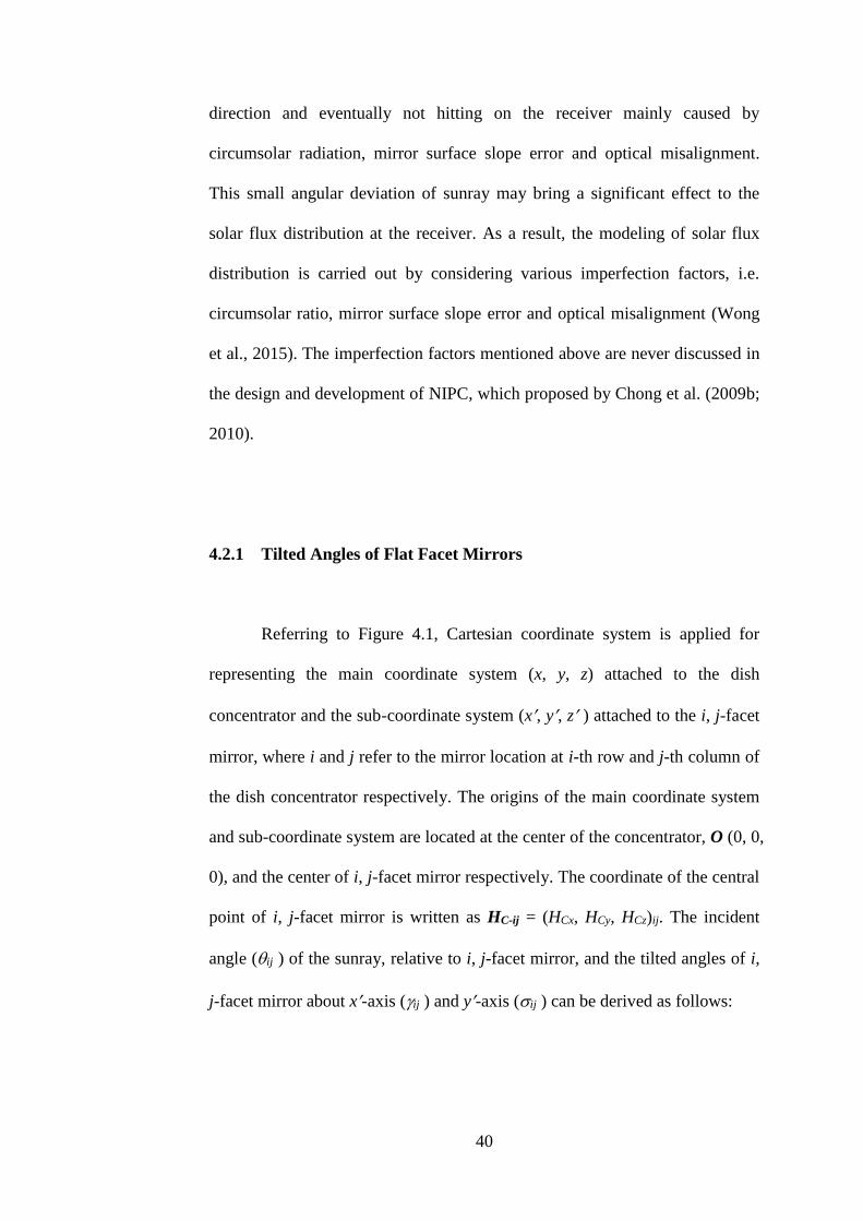
4.2.1 Tilted Angles of Flat Facet Mirrors

Referring to Figure 4.1, Cartesian coordinate system is applied for

representing the main coordinate system (x, y, z) attached to the dish

concentrator and the sub-coordinate system (x, y, z ) attached to the i, j-facet

mirror, where i and j refer to the mirror location at i-th row and j-th column of

the dish concentrator respectively. The origins of the main coordinate system

and sub-coordinate system are located at the center of the concentrator, O (0, 0,

0), and the center of i, j-facet mirror respectively. The coordinate of the central

point of i, j-facet mirror is written as HC-ij = (HCx, HCy, HCz)ij. The incident

angle (ij ) of the sunray, relative to i, j-facet mirror, and the tilted angles of i,

j-facet mirror about x-axis (ij ) and y-axis (ij ) can be derived as follows:

41

2 21

arctan2

Cx Cy

ij

Czij

H H

f H

(4.1)

22 2

arctan Cxij

Cz Cx Cy Czij

H

f H H H f H

(4.2)

22 2

22 2

arctan

2 2

2

Cxij

Cx Cy Cz

Cz Cx Cy Czij

H

H H f H

f H H H f H

(4.3)

where f is the focal length of the dish concentrator or the perpendicular

distance of central points between the dish concentrator and the receiver.

Figure 4.1: The Cartesian coordinate system used to represent the main

coordinate system (x, y, z) attached to the plane of the dish concentrator and the

sub-coordinate system (x, y, z) is defined attached to the i, j-facet mirror.

42

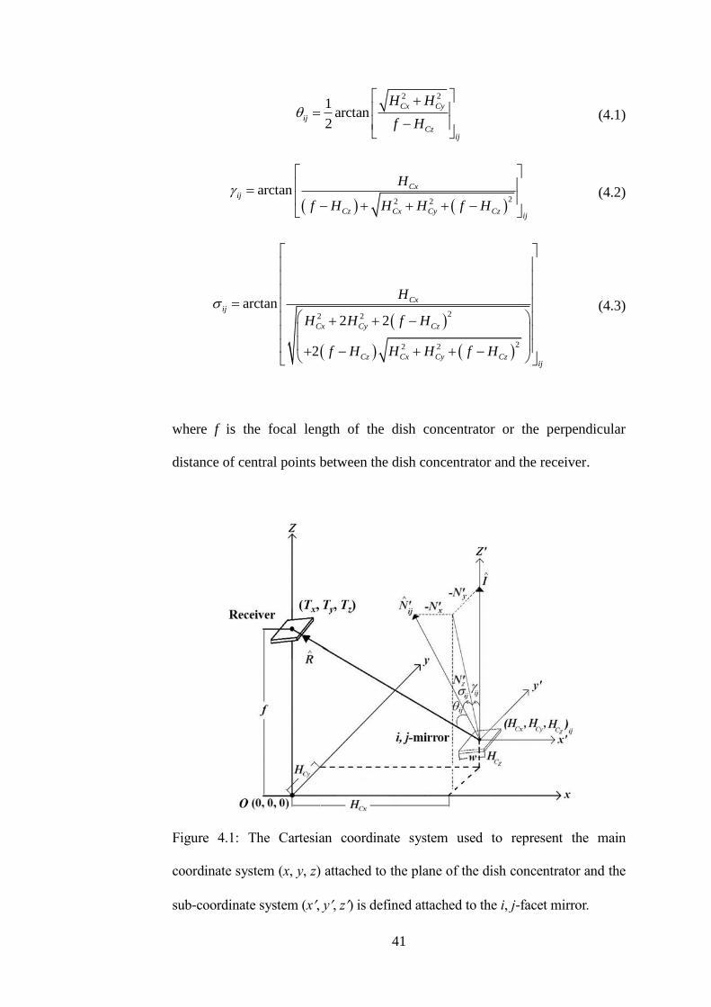
According to the principle of NIDC, all the flat facet mirrors need to be

aligned precisely to produce a uniform solar flux distribution through the

superposition of all the sunlight on the receiver. In fact, it is an arduous work

to achieve perfect optical alignment in the flat facet mirrors of the concentrator.

After the solar concentrator has been constructed, there are many factors to

induce the optical misalignment of facet mirrors, which include manufacturing

defect, imperfect optical alignment, and self-weight mechanical deflection.

The induced optical misalignment makes the normal axis of the facet mirror

deviated from its ideal orientation. The deviation of the normal axis of facet

mirror can contribute to the distortion of the solar flux distribution. As shown

in Figure 4.2, the optical misalignment angles of each facet mirror are

introduced in the numerical modeling of the NIDC prototype in which the new

tilted angles of i, j-facet mirror about x-axis ( 'ij) and y-axis ( 'ij) can be

calculated by using the following expressions:

1 1ij ij r r

(4.4)

1 1ij ij r r

(4.5)

where r and r are the pseudorandom numbers, is the optical misalignment

angle of the mirror, ij and ij are the tilted angles of i, j-facet mirror about x-

axis and y-axis respectively without considering the optical misalignment.

43

Figure 4.2: Two new tilted angles of i, j-facet mirror about x-axis (ij ) and y-

axis (ij ) caused by optical misalignment.

4.2.2 Coordinate Transformation

An initial coordinate of the reflective point on the i, j-facet mirror is

designated as Hijkl = (Hx, Hy, Hz)ijkl, where k and l represent the position of the

reflective point at the k-th row and l-th column of the facet mirror respectively.

To ease the mathematical representation of coordinate transformations, we can

make the translation a linear transformation by increasing the dimensionality

of space. Thus, the coordinates (Hx, Hy, Hz)ijkl can also be represented by (Hx,

Hy, Hz, 1)ijkl, which is also treated as a vector in matrix form

1

x

y

ijklz

ijkl

H

HH

H

(4.6)

44

A new coordinate Hijkl = (Hx, Hy, Hz)ijkl is formed when each mirror has to

be aligned with its corresponding tilted angles ( 'ij and 'ij) for superposing

all the incident sunlight at the common receiver. The final position of

reflective point can also be written in a matrix form as

1

x

y

ijklz

ijkl

H

HH

H

(4.7)

If the pivot point of the i, j-facet mirror (HCx, HCy, HCz)ij is not located

at the origin of the main coordinate system, the reflective point will be treated

under translation transformation before rotation transformations. The initial

coordinates of the reflective point will be first transformed from the main

coordinate system that is attached to the concentrator frame to the sub-

coordinate system that is attached to the local facet mirror via a translation

transformation. The translation transformation matrix is

1

1 0 0

0 1 0

0 0 1

0 0 0 1

Cx

Cy

ijCz

ij

H

HT

H

(4.8)

Then, it is followed by the first rotation transformation with the angle 'ij

about the y-axis of the sub-coordinated system to transform the reflective point

from the sub-coordinate system to a column movement coordinate system.

The first rotation transformation matrix can be written as

45

cos 0 sin 0

0 1 0 0

sin 0 cos 0

0 0 0 1

ij ij

ij

ij ij

(4.9)

The following second rotation transformation with the angle 'ij about the x-

axis of the column movement coordinate system transforms the reflective

point from the column movement coordinate system to a row movement

coordinate system. The second rotation transformation matrix can be written

as

1 0 0 0

0 cos sin 0

0 sin cos 0

0 0 0 1

ij ij

ij

ij ij

(4.10)

Finally, to transform the row movement coordinate system back to the main

coordinate system, we need the last translation matrix that is written as

2

1 0 0

0 1 0

0 0 1

0 0 0 1

Cx

Cy

ijCz

ij

H

HT

H

(4.11)

As a result, the matrix for the coordinate transformations from the initial

coordinate Hijkl = (Hx, Hy, Hz)ijkl to the final coordinate Hijkl = (Hx, Hy, Hz)ijkl

can be shortly represented as

46

2 1ij ijijkl ij ij ijklH T T H (4.12)

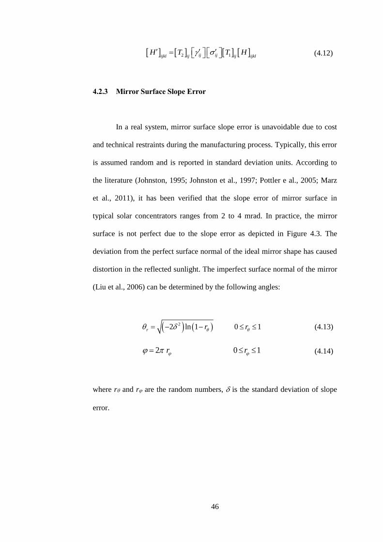
4.2.3 Mirror Surface Slope Error

In a real system, mirror surface slope error is unavoidable due to cost

and technical restraints during the manufacturing process. Typically, this error

is assumed random and is reported in standard deviation units. According to

the literature (Johnston, 1995; Johnston et al., 1997; Pottler e al., 2005; Marz

et al., 2011), it has been verified that the slope error of mirror surface in

typical solar concentrators ranges from 2 to 4 mrad. In practice, the mirror

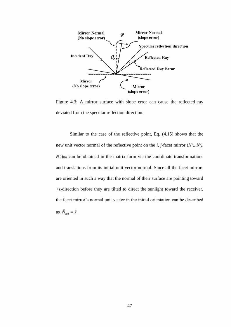
surface is not perfect due to the slope error as depicted in Figure 4.3. The

deviation from the perfect surface normal of the ideal mirror shape has caused

distortion in the reflected sunlight. The imperfect surface normal of the mirror

(Liu et al., 2006) can be determined by the following angles:

22 ln 1 0 1r r r (4.13)

2 0 1r r (4.14)

where r and r are the random numbers, is the standard deviation of slope

error.

47

Figure 4.3: A mirror surface with slope error can cause the reflected ray

deviated from the specular reflection direction.

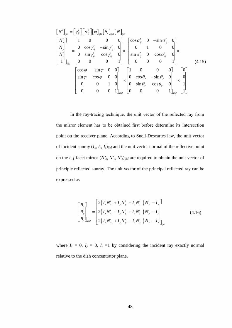
Similar to the case of the reflective point, Eq. (4.15) shows that the

new unit vector normal of the reflective point on the i, j-facet mirror (Nx, Ny,

Nz)ijkl can be obtained in the matrix form via the coordinate transformations

and translations from its initial unit vector normal. Since all the facet mirrors

are oriented in such a way that the normal of their surface are pointing toward

+z-direction before they are tilted to direct the sunlight toward the receiver,

the facet mirror’s normal unit vector in the initial orientation can be described

as ˆ ˆijklN z .

48

1 0 0 0 cos 0 sin 0

0 cos sin 0 0 1 0 0

0 sin cos 0 sin 0 cos 0

1 0 0 0 1 0 0 0 1

cos sin 0

ij ij rijkl ijkl ijkl ijkl

x ij ij

y ij ij

z ij ij ij ij

ijkl

N N

N

N

N

0 1 0 0 0 0

sin cos 0 0 0 cos sin 0 0

0 0 1 0 0 sin cos 0 1

0 0 0 1 0 0 0 1 1

r r

r r

ijkl ijkl

(4.15)

In the ray-tracing technique, the unit vector of the reflected ray from

the mirror element has to be obtained first before determine its intersection

point on the receiver plane. According to Snell-Descartes law, the unit vector

of incident sunray (Ix, Iy, Iz)ijkl and the unit vector normal of the reflective point

on the i, j-facet mirror (Nx, Ny, Nz)ijkl are required to obtain the unit vector of

principle reflected sunray. The unit vector of the principal reflected ray can be

expressed as

2

2

2

x x y y z z x xx

y x x y y z z y y

z ijklx x y y z z z z

ijkl

I N I N I N N IR

R I N I N I N N I

R I N I N I N N I

(4.16)

where Ix = 0, Iy = 0, Iz =1 by considering the incident ray exactly normal

relative to the dish concentrator plane.

49

4.2.4 Circumsolar Radiation

In addition to mirror slope error, circumsolar radiation also contributes

to the distortion of the flux distribution cast on the receiver. Buie et al. (2003a;

2003b) showed that the amount of energy in the circumsolar region is

important because sun-shape plays an important role in determining the

overall flux distribution and overestimated of output power may occur if all

the power is assumed to fall within the extent of the solar disc only. The

seriousness of circumsolar radiation effect is rated in term of the circumsolar

ratio (CSR). Noring et al. (1991) demonstrated that the CSR values typically

vary in the range from zero to 0.3. Circumsolar radiation is also considered in

the optical analysis of the dish concentrator, where the solar rays that strike the

mirror surface and the receiver are treated as cone rays.

In order to study the influence of circumsolar radiation to the solar flux

distribution, for each principal reflected sunray, ˆijklR , P sub-rays are generated

within the solar cone, which subtends to the effective half angle of 43.6 mrad

(Buie et al., 2003a; Buie et al., 2003b). Each sub-ray is denoted as

ˆ 垐 ˆm mx my mzR R x R y R z , where m = 1, 2, 3,…P. By solving the line equation

of the sub-ray and the surface equation of the receiver plane, the coordinate of

the intersection point on the receiver can be calculated as

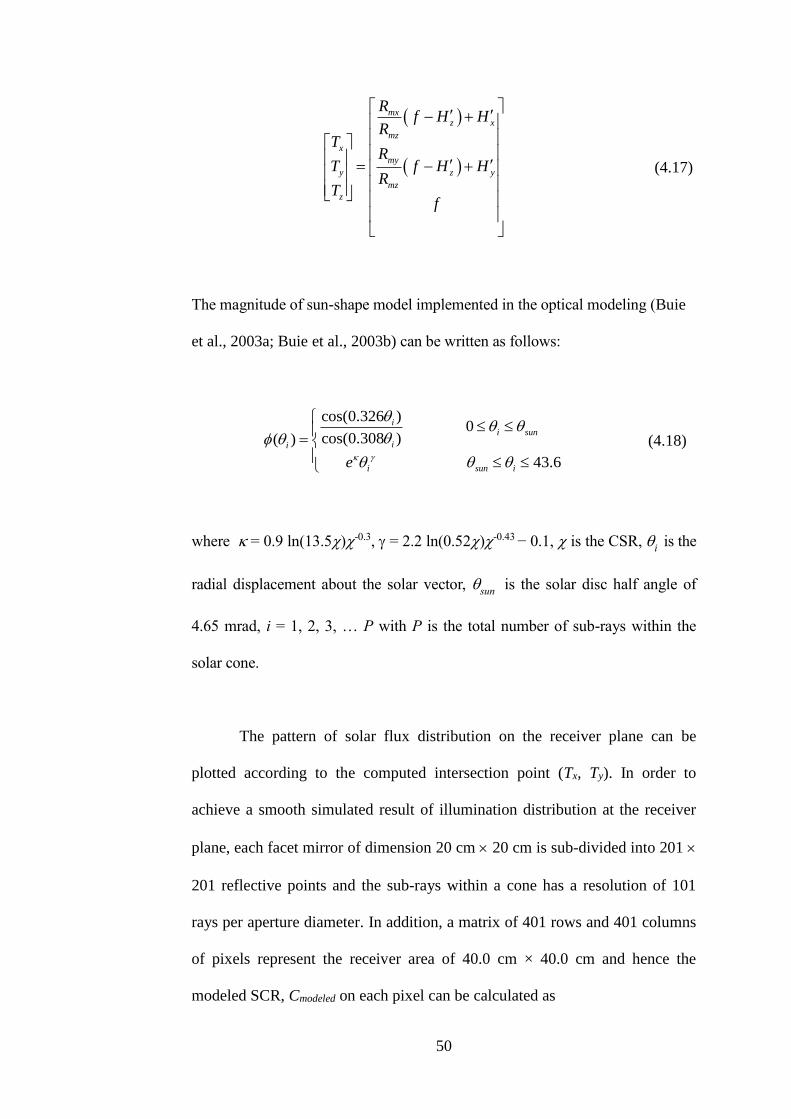
50

mxz x

mz

x

my

y z y

mz

z

Rf H H

RT

RT f H H

RT

f

(4.17)

The magnitude of sun-shape model implemented in the optical modeling (Buie

et al., 2003a; Buie et al., 2003b) can be written as follows:

cos(0.326 )0

cos(0.308 )( )

43.6

ii sun

ii

i sun ie

(4.18)

where = 0.9 ln(13.5)-0.3, = 2.2 ln(0.52)-0.43 − 0.1, is the CSR, i is the

radial displacement about the solar vector, sun is the solar disc half angle of

4.65 mrad, i = 1, 2, 3, … P with P is the total number of sub-rays within the

solar cone.

The pattern of solar flux distribution on the receiver plane can be

plotted according to the computed intersection point (Tx, Ty). In order to

achieve a smooth simulated result of illumination distribution at the receiver

plane, each facet mirror of dimension 20 cm 20 cm is sub-divided into 201

201 reflective points and the sub-rays within a cone has a resolution of 101

rays per aperture diameter. In addition, a matrix of 401 rows and 401 columns

of pixels represent the receiver area of 40.0 cm × 40.0 cm and hence the

modeled SCR, Cmodeled on each pixel can be calculated as

51

2

mod 21

1

area of reflective point (cm ) cos

area of receiver pixel (cm )

N

eled i Pn

i

i

C

(4.19)

where the area of a reflective point = (20/201)2, the area of a receiver pixel =

(40/401)2, N is the total count of sub-rays hitting on the corresponding pixel on

the receiver plane.

4.3 Results and Discussions

In this study, an optical characterization of the prototype of NIDC has

been carried out using the aforementioned ray-tracing method by changing the

values of optical misalignment angle () in the range from 0 to 0.4,

circumsolar ratio () in the range from 0 to 0.4, and, mirror surface slope error

() in the range from 0 to 4 mrad. Figure 4.4 shows the simulated results of

solar flux distribution of NIDC in 2-D and 3-D mesh plots provided that all the

parameters, i.e. , and , are null. By omitting the imperfection factors, the

NIDC is capable of producing 338 cm2 of uniform illumination area, which

consists of a flat top area in the central region of flux distribution where the

SCR is nearly constant, with a maximum SCR of 88 suns at the receiver.

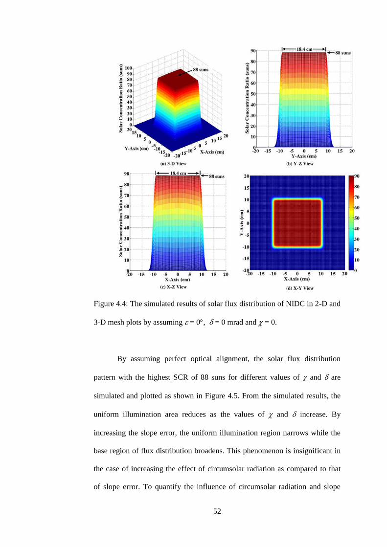
52

Figure 4.4: The simulated results of solar flux distribution of NIDC in 2-D and

3-D mesh plots by assuming = 0, = 0 mrad and = 0.

By assuming perfect optical alignment, the solar flux distribution

pattern with the highest SCR of 88 suns for different values of and are

simulated and plotted as shown in Figure 4.5. From the simulated results, the

uniform illumination area reduces as the values of and increase. By

increasing the slope error, the uniform illumination region narrows while the

base region of flux distribution broadens. This phenomenon is insignificant in

the case of increasing the effect of circumsolar radiation as compared to that

of slope error. To quantify the influence of circumsolar radiation and slope

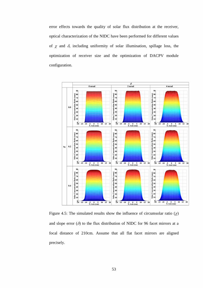
53

error effects towards the quality of solar flux distribution at the receiver,

optical characterization of the NIDC have been performed for different values

of and , including uniformity of solar illumination, spillage loss, the

optimization of receiver size and the optimization of DACPV module

configuration.

Figure 4.5: The simulated results show the influence of circumsolar ratio ()

and slope error () to the flux distribution of NIDC for 96 facet mirrors at a

focal distance of 210cm. Assume that all flat facet mirrors are aligned

precisely.

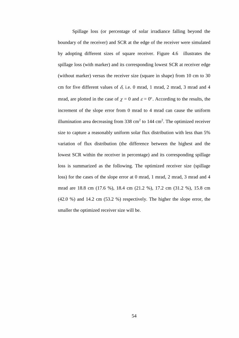
54

Spillage loss (or percentage of solar irradiance falling beyond the

boundary of the receiver) and SCR at the edge of the receiver were simulated

by adopting different sizes of square receiver. Figure 4.6 illustrates the

spillage loss (with marker) and its corresponding lowest SCR at receiver edge

(without marker) versus the receiver size (square in shape) from 10 cm to 30

cm for five different values of , i.e. 0 mrad, 1 mrad, 2 mrad, 3 mrad and 4

mrad, are plotted in the case of = 0 and = 0. According to the results, the

increment of the slope error from 0 mrad to 4 mrad can cause the uniform

illumination area decreasing from 338 cm2 to 144 cm2. The optimized receiver

size to capture a reasonably uniform solar flux distribution with less than 5%

variation of flux distribution (the difference between the highest and the

lowest SCR within the receiver in percentage) and its corresponding spillage

loss is summarized as the following. The optimized receiver size (spillage

loss) for the cases of the slope error at 0 mrad, 1 mrad, 2 mrad, 3 mrad and 4

mrad are 18.8 cm (17.6 %), 18.4 cm (21.2 %), 17.2 cm (31.2 %), 15.8 cm

(42.0 %) and 14.2 cm (53.2 %) respectively. The higher the slope error, the

smaller the optimized receiver size will be.

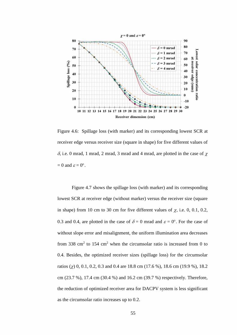
55

Figure 4.6: Spillage loss (with marker) and its corresponding lowest SCR at

receiver edge versus receiver size (square in shape) for five different values of

, i.e. 0 mrad, 1 mrad, 2 mrad, 3 mrad and 4 mrad, are plotted in the case of

= 0 and = 0.

Figure 4.7 shows the spillage loss (with marker) and its corresponding

lowest SCR at receiver edge (without marker) versus the receiver size (square

in shape) from 10 cm to 30 cm for five different values of , i.e. 0, 0.1, 0.2,

0.3 and 0.4, are plotted in the case of = 0 mrad and = 0. For the case of

without slope error and misalignment, the uniform illumination area decreases

from 338 cm2 to 154 cm2 when the circumsolar ratio is increased from 0 to

0.4. Besides, the optimized receiver sizes (spillage loss) for the circumsolar

ratios () 0, 0.1, 0.2, 0.3 and 0.4 are 18.8 cm (17.6 %), 18.6 cm (19.9 %), 18.2

cm (23.7 %), 17.4 cm (30.4 %) and 16.2 cm (39.7 %) respectively. Therefore,

the reduction of optimized receiver area for DACPV system is less significant

as the circumsolar ratio increases up to 0.2.

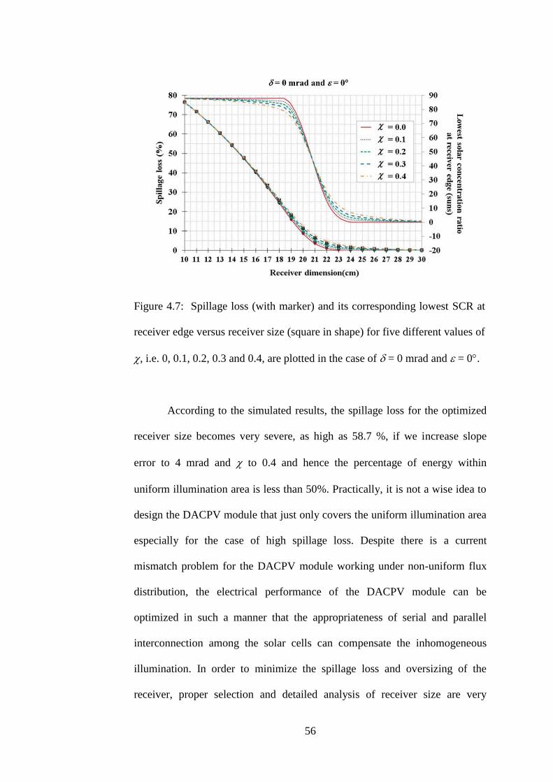
56



, i.e. 0, 0.1, 0.2, 0.3 and 0.4, are plotted in the case of = 0 mrad and = 0.

According to the simulated results, the spillage loss for the optimized

receiver size becomes very severe, as high as 58.7 %, if we increase slope

error to 4 mrad and to 0.4 and hence the percentage of energy within

uniform illumination area is less than 50%. Practically, it is not a wise idea to

design the DACPV module that just only covers the uniform illumination area

especially for the case of high spillage loss. Despite there is a current

mismatch problem for the DACPV module working under non-uniform flux

distribution, the electrical performance of the DACPV module can be

optimized in such a manner that the appropriateness of serial and parallel

interconnection among the solar cells can compensate the inhomogeneous

illumination. In order to minimize the spillage loss and oversizing of the

receiver, proper selection and detailed analysis of receiver size are very

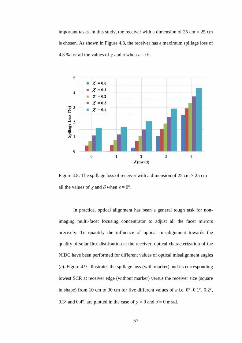
57

important tasks. In this study, the receiver with a dimension of 25 cm × 25 cm

is chosen. As shown in Figure 4.8, the receiver has a maximum spillage loss of

4.3 % for all the values of and when = 0.

Figure 4.8: The spillage loss of receiver with a dimension of 25 cm × 25 cm

all the values of and when = 0.

In practice, optical alignment has been a general tough task for non-

imaging multi-facet focusing concentrator to adjust all the facet mirrors

precisely. To quantify the influence of optical misalignment towards the

quality of solar flux distribution at the receiver, optical characterization of the

NIDC have been performed for different values of optical misalignment angles

(). Figure 4.9 illustrates the spillage loss (with marker) and its corresponding

lowest SCR at receiver edge (without marker) versus the receiver size (square

in shape) from 10 cm to 30 cm for five different values of i.e. 0, 0.1, 0.2,

0.3 and 0.4, are plotted in the case of = 0 and = 0 mrad.

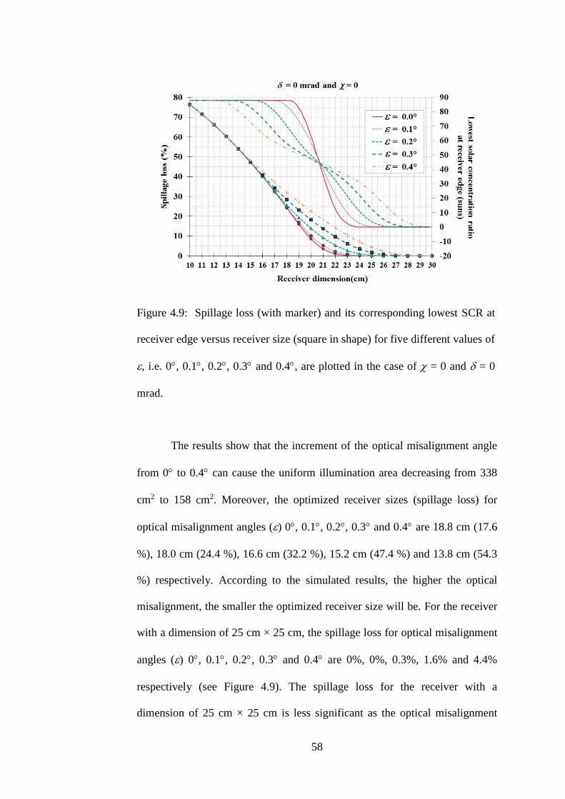
58



, i.e. 0, 0.1, 0.2, 0.3 and 0.4, are plotted in the case of = 0 and = 0

mrad.

The results show that the increment of the optical misalignment angle

from 0 to 0.4 can cause the uniform illumination area decreasing from 338

cm2 to 158 cm2. Moreover, the optimized receiver sizes (spillage loss) for

optical misalignment angles () 0, 0.1, 0.2, 0.3 and 0.4 are 18.8 cm (17.6

%), 18.0 cm (24.4 %), 16.6 cm (32.2 %), 15.2 cm (47.4 %) and 13.8 cm (54.3

%) respectively. According to the simulated results, the higher the optical

misalignment, the smaller the optimized receiver size will be. For the receiver

with a dimension of 25 cm × 25 cm, the spillage loss for optical misalignment

angles () 0, 0.1, 0.2, 0.3 and 0.4 are 0%, 0%, 0.3%, 1.6% and 4.4%

respectively (see Figure 4.9). The spillage loss for the receiver with a

dimension of 25 cm × 25 cm is less significant as the optical misalignment

59

angles increase up to 0.2. As a result, an accurate, inexpensive and fast

approach is necessary to align the facet mirrors of the solar concentrator for

minimizing the distortion of solar flux distribution.

4.4 Summary

A numerical simulation using ray-tracing method to model the solar

flux distribution of NIDC prototype has been developed by considering three

imperfection factors, i.e., circumsolar ratio, mirror slope error and optical

misalignment. A comprehensive analysis on the simulation results has been

carried out by considering all the important criteria to optimize the

performance of DACPV system, such as the maximum SCR, uniform

illumination area, and spillage loss. According to the simulated results, the

three imperfection factors can cause serious deterioration to the uniform flux

distribution area and the percentage of energy within the uniform illumination

area. It is not a wise idea to design the DACPV module that just only covers

the uniform illumination area. Therefore, the receiver size of a DACPV

system can be optimized with the simulated flux distribution by minimizing

the spillage loss. In this study, the receiver with a dimension of 25 cm × 25 cm

is chosen to capture more than 95% of solar irradiance.

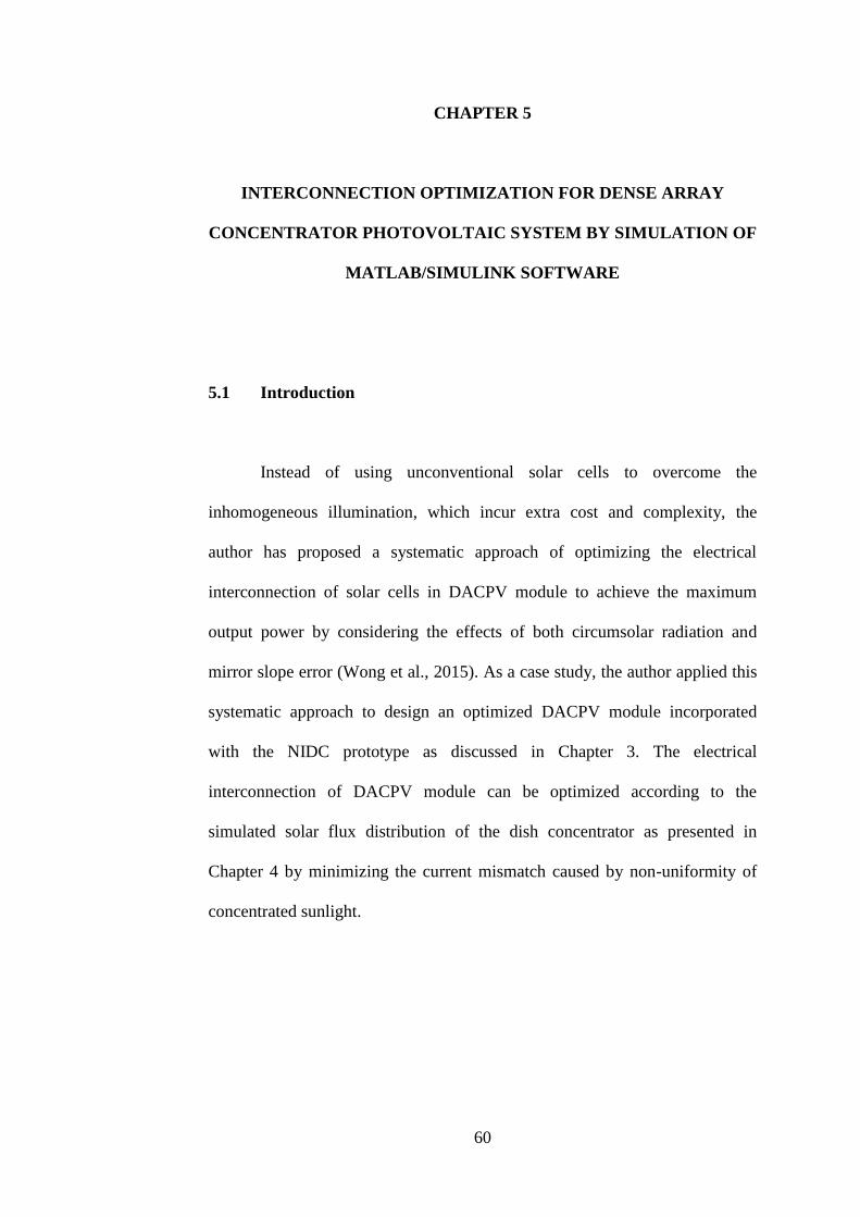
60

CHAPTER 5

INTERCONNECTION OPTIMIZATION FOR DENSE ARRAY

CONCENTRATOR PHOTOVOLTAIC SYSTEM BY SIMULATION OF

MATLAB/SIMULINK SOFTWARE

5.1 Introduction

Instead of using unconventional solar cells to overcome the

inhomogeneous illumination, which incur extra cost and complexity, the

author has proposed a systematic approach of optimizing the electrical

interconnection of solar cells in DACPV module to achieve the maximum

output power by considering the effects of both circumsolar radiation and

mirror slope error (Wong et al., 2015). As a case study, the author applied this

systematic approach to design an optimized DACPV module incorporated

with the NIDC prototype as discussed in Chapter 3. The electrical

interconnection of DACPV module can be optimized according to the

simulated solar flux distribution of the dish concentrator as presented in

Chapter 4 by minimizing the current mismatch caused by non-uniformity of

concentrated sunlight.

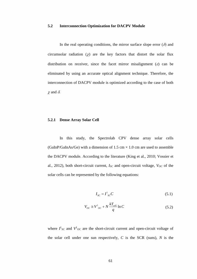
61

5.2 Interconnection Optimization for DACPV Module

In the real operating conditions, the mirror surface slope error ( and

circumsolar radiation () are the key factors that distort the solar flux

distribution on receiver, since the facet mirror misalignment () can be

eliminated by using an accurate optical alignment technique. Therefore, the

interconnection of DACPV module is optimized according to the case of both

and

5.2.1 Dense Array Solar Cell

In this study, the Spectrolab CPV dense array solar cells

(GaInP/GaInAs/Ge) with a dimension of 1.5 cm × 1.0 cm are used to assemble

the DACPV module. According to the literature (King et al., 2010; Vossier et

al., 2012), both short-circuit current, ISC and open-circuit voltage, VOC of the

solar cells can be represented by the following equations:

1

SC SCI I C (5.1)

1 lncellOC OC

kTV V N C

q (5.2)

where I1SC and V1

OC are the short-circuit current and open-circuit voltage of

the solar cell under one sun respectively, C is the SCR (suns), N is the

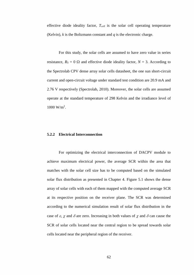
62

effective diode ideality factor, Tcell is the solar cell operating temperature

(Kelvin), k is the Boltzmann constant and q is the electronic charge.

For this study, the solar cells are assumed to have zero value in series

resistance, RS = 0 and effective diode ideality factor, N = 3. According to

the Spectrolab CPV dense array solar cells datasheet, the one sun short-circuit

current and open-circuit voltage under standard test condition are 20.9 mA and

2.76 V respectively (Spectrolab, 2010). Moreover, the solar cells are assumed

operate at the standard temperature of 298 Kelvin and the irradiance level of

1000 W/m2.

5.2.2 Electrical Interconnection

For optimizing the electrical interconnection of DACPV module to

achieve maximum electrical power, the average SCR within the area that

matches with the solar cell size has to be computed based on the simulated

solar flux distribution as presented in Chapter 4. Figure 5.1 shows the dense

array of solar cells with each of them mapped with the computed average SCR

at its respective position on the receiver plane. The SCR was determined

according to the numerical simulation result of solar flux distribution in the

case of , and are zero. Increasing in both values of and can cause the

SCR of solar cells located near the central region to be spread towards solar

cells located near the peripheral region of the receiver.

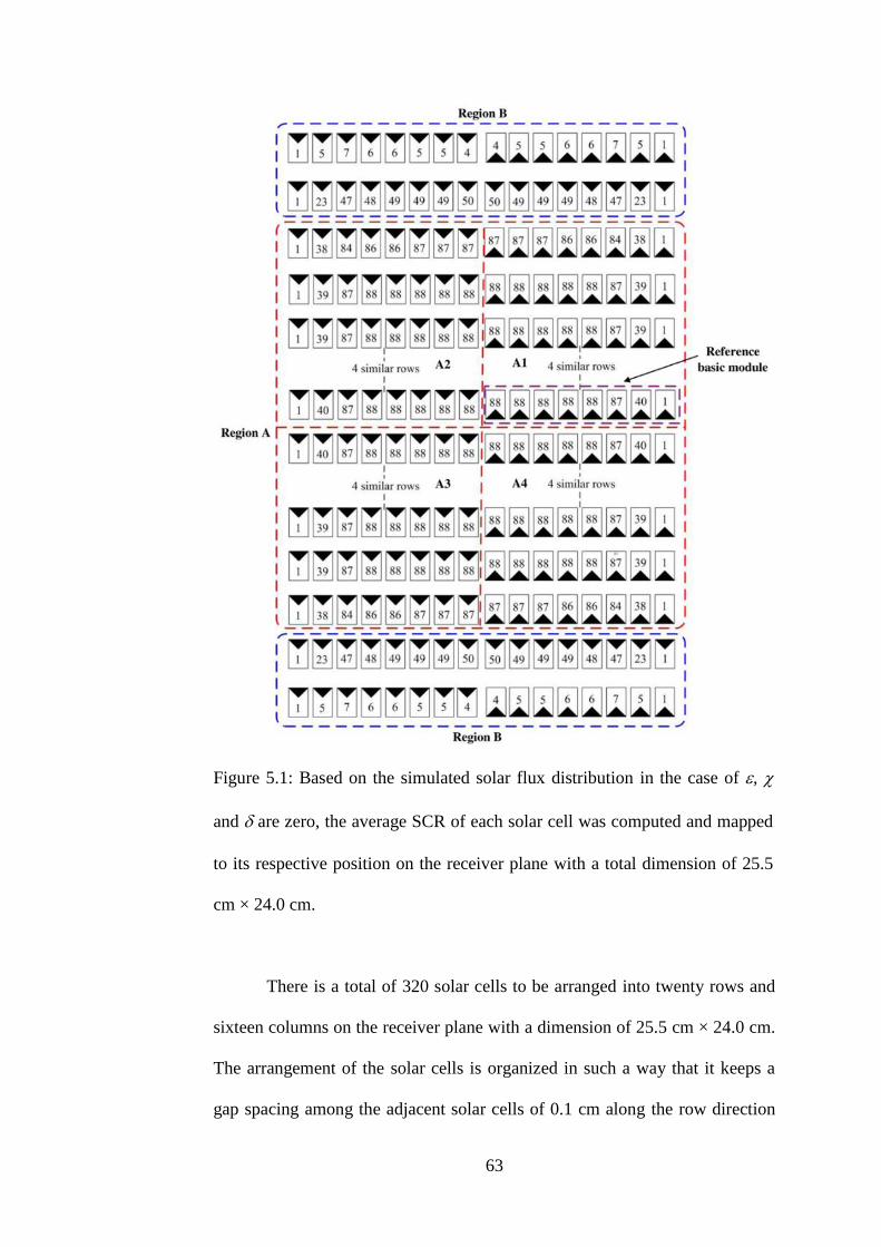
63

Figure 5.1: Based on the simulated solar flux distribution in the case of ,

and are zero, the average SCR of each solar cell was computed and mapped

to its respective position on the receiver plane with a total dimension of 25.5

cm × 24.0 cm.

There is a total of 320 solar cells to be arranged into twenty rows and

sixteen columns on the receiver plane with a dimension of 25.5 cm × 24.0 cm.

The arrangement of the solar cells is organized in such a way that it keeps a

gap spacing among the adjacent solar cells of 0.1 cm along the row direction

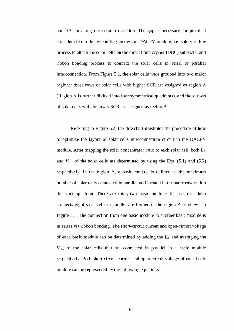
64

and 0.2 cm along the column direction. The gap is necessary for practical

consideration in the assembling process of DACPV module, i.e. solder reflow

process to attach the solar cells on the direct bond copper (DBC) substrate, and

ribbon bonding process to connect the solar cells in serial or parallel

interconnection. From Figure 5.1, the solar cells were grouped into two major

regions: those rows of solar cells with higher SCR are assigned as region A

(Region A is further divided into four symmetrical quadrants), and those rows

of solar cells with the lower SCR are assigned as region B.

Referring to Figure 5.2, the flowchart illustrates the procedure of how

to optimize the layout of solar cells interconnection circuit in the DACPV

module. After mapping the solar concentrator ratio to each solar cell, both ISC

and VOC of the solar cells are determined by using the Eqs. (5.1) and (5.2)

respectively. In the region A, a basic module is defined as the maximum

number of solar cells connected in parallel and located in the same row within

the same quadrant. There are thirty-two basic modules that each of them

connects eight solar cells in parallel are formed in the region A as shown in

Figure 5.1. The connection from one basic module to another basic module is

in series via ribbon bonding. The short-circuit current and open-circuit voltage

of each basic module can be determined by adding the ISC and averaging the

VOC of the solar cells that are connected in parallel in a basic module

respectively. Both short-circuit current and open-circuit voltage of each basic

module can be represented by the following equations:

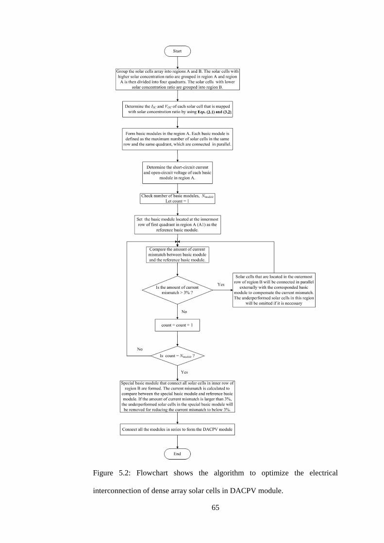
65

Figure 5.2: Flowchart shows the algorithm to optimize the electrical

interconnection of dense array solar cells in DACPV module.

66

SC module

1

n

SCI I (5.3)

1O module

n

OC

C

V

Vn

(5.4)

where ISC and VOC are the short-circuit current and open-circuit voltage of single

solar cell accordingly, and n is the number of solar cells connected in parallel in

a basic module.

The basic module located in the innermost row of the quadrant in the

region A is set as the reference basic module. For example, reference basic

module is selected in the region A1 as shown in Figure 5.1. The current

mismatch is computed to compare the amount of output current between the

other basic modules and the reference basic module. If the amount of current

mismatch is larger than 3 %, the algorithm will select solar cells that are

located in the outermost row of region B to connect in parallel externally with

the corresponding basic modules for reducing the current mismatch to below

3%. Those solar cells in the outermost row of region B that is not utilized for

compensating current mismatch will be removed at the end of the optimization

process.

The subsequent row of solar cells after the outermost row in region B

is defined as a special basic module in which all solar cells are connected in

parallel. The current mismatch is also calculated to compare with the reference

basic module. If the amount of current mismatch is larger than 3%, the

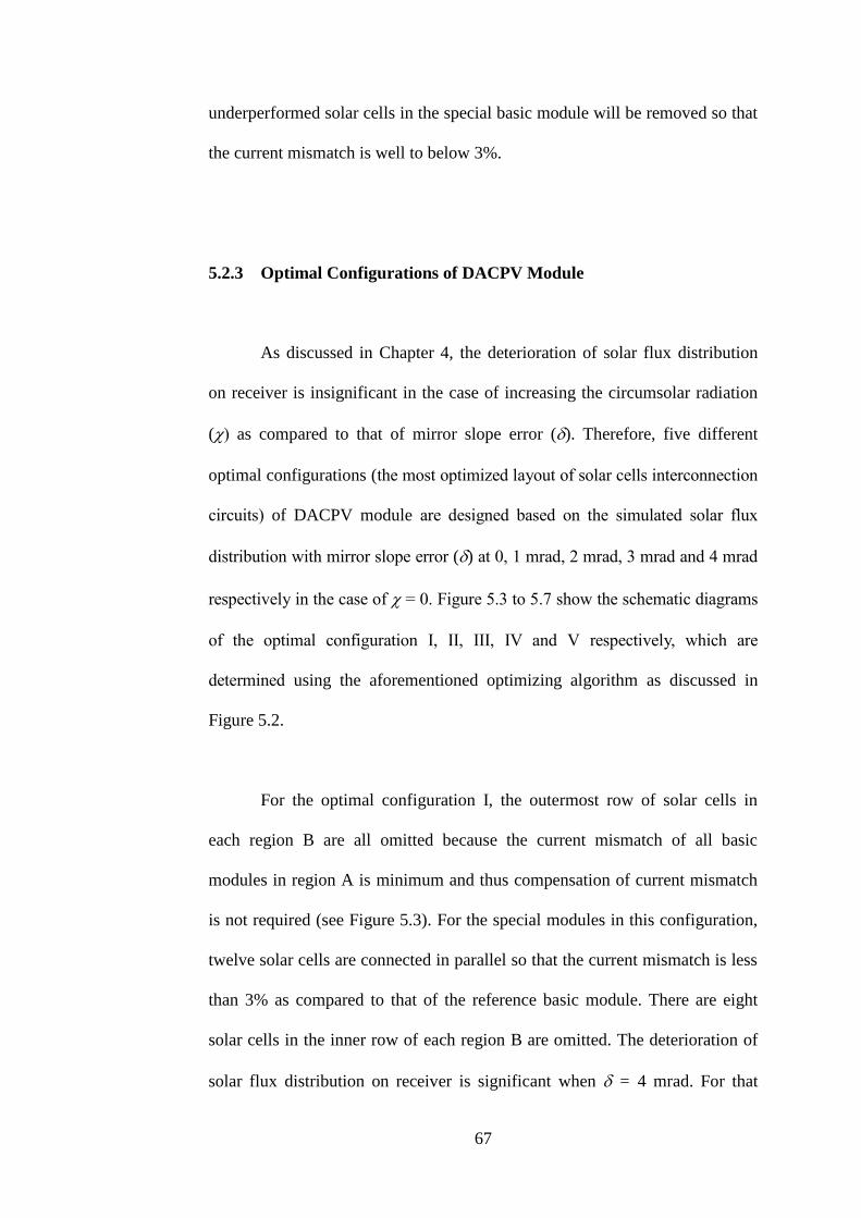
67

underperformed solar cells in the special basic module will be removed so that

the current mismatch is well to below 3%.

5.2.3 Optimal Configurations of DACPV Module

As discussed in Chapter 4, the deterioration of solar flux distribution

on receiver is insignificant in the case of increasing the circumsolar radiation

() as compared to that of mirror slope error (). Therefore, five different

optimal configurations (the most optimized layout of solar cells interconnection

circuits) of DACPV module are designed based on the simulated solar flux

distribution with mirror slope error () at 0, 1 mrad, 2 mrad, 3 mrad and 4 mrad

respectively in the case of = 0. Figure 5.3 to 5.7 show the schematic diagrams

of the optimal configuration I, II, III, IV and V respectively, which are

determined using the aforementioned optimizing algorithm as discussed in

Figure 5.2.

For the optimal configuration I, the outermost row of solar cells in

each region B are all omitted because the current mismatch of all basic

modules in region A is minimum and thus compensation of current mismatch

is not required (see Figure 5.3). For the special modules in this configuration,

twelve solar cells are connected in parallel so that the current mismatch is less

than 3% as compared to that of the reference basic module. There are eight

solar cells in the inner row of each region B are omitted. The deterioration of

solar flux distribution on receiver is significant when = 4 mrad. For that

68

reason, in the optimal configuration V, there are eight basic modules in region

A being connected in parallel externally with all solar cells that are located in

the outermost row of region B for reducing the current mismatch to below 3%

as compared to that of the reference basic module (see Figure 5.7). In addition,

fourteen solar cells located in the innermost row of each region B are

connected in parallel externally to form the special modules in the optimal

configuration V. There are two solar cells in the inner row of each region B

are omitted.

By comparing the schematic diagrams shown in Figure 5.3 to 5.7, the

number of solar cells used is increased for designing the optimized layout of

solar cell interconnection circuits as the value of is increased. The

deteriorated solar flux distribution on receiver requires more solar cells for

compensating the current mismatch among the basic modules. As the value of

is increased, the solar cells near to the peripheral region of the receiver will

receive additional solar flux. At the same time, the flux density around the

central region is reduced. Therefore, the number of solar cells in the basic

module that near to the peripheral has to be increased in order to make up the

current mismatch to be less than 3 %. The number of solar cells used in

optimal configuration I, II, III, IV and V are 280, 288, 296, 308 and 316

respectively.

69

Figure 5.3: Schematic diagram to show optimal configuration I for the case of

= 0 mrad and = 0.

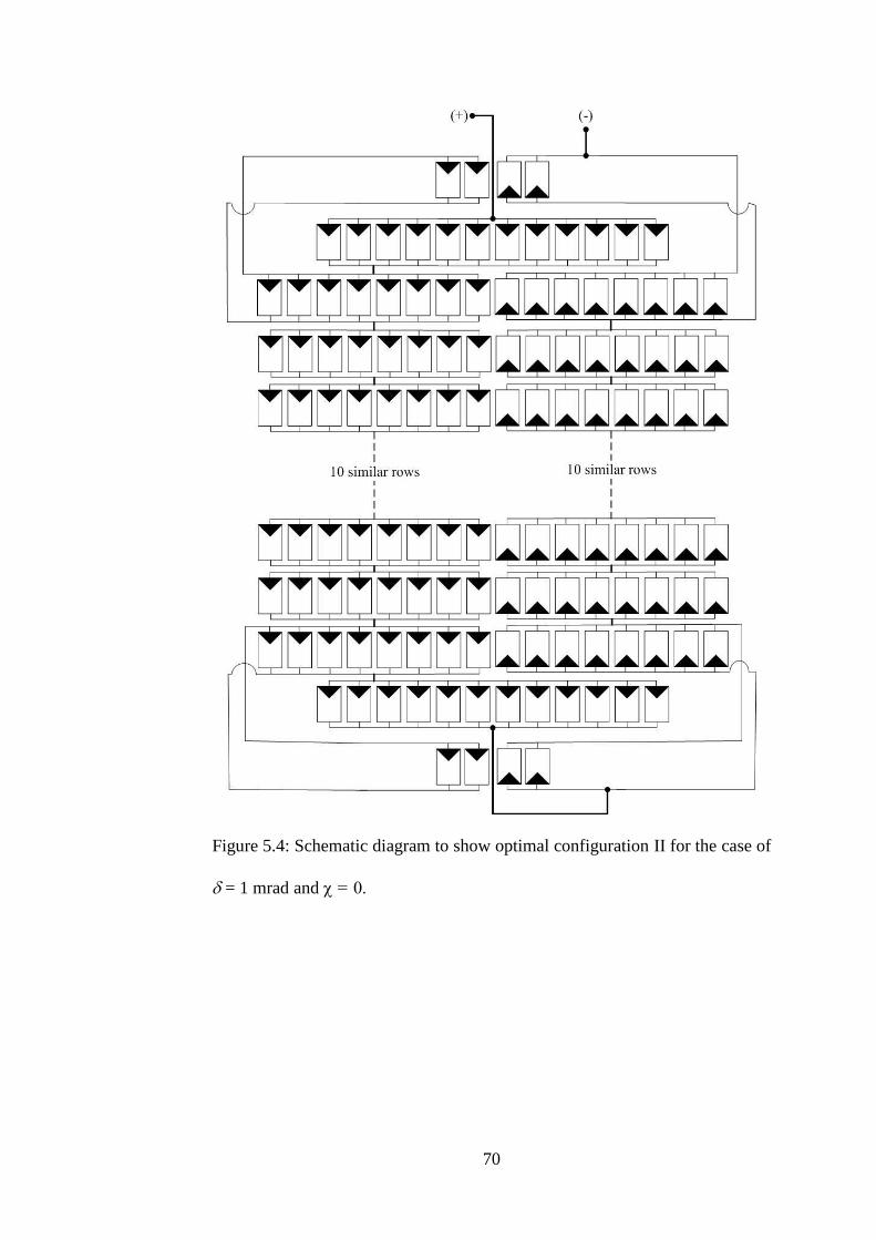
70

Figure 5.4: Schematic diagram to show optimal configuration II for the case of

= 1 mrad and = 0.

71

Figure 5.5: Schematic diagram to show optimal configuration III for the case

of = 2 mrad and = 0.

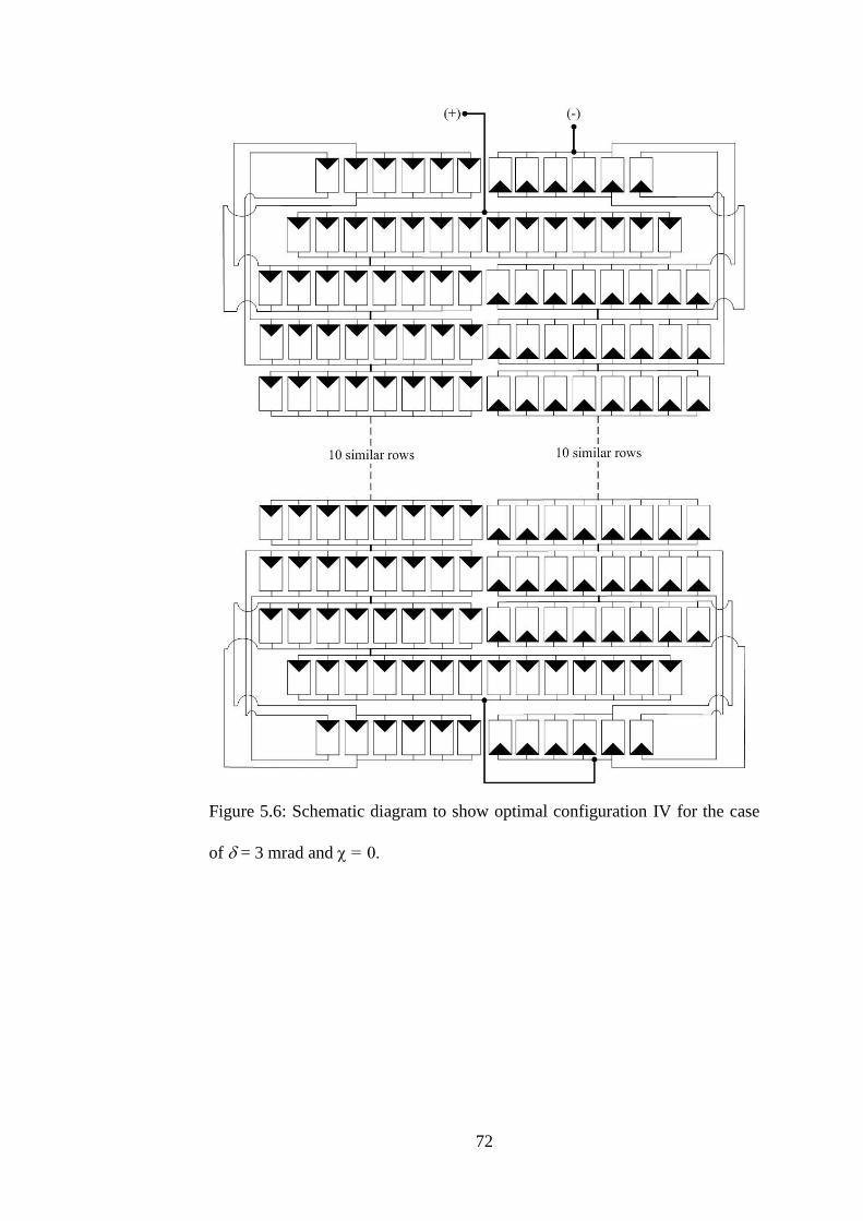
72

Figure 5.6: Schematic diagram to show optimal configuration IV for the case

of = 3 mrad and = 0.

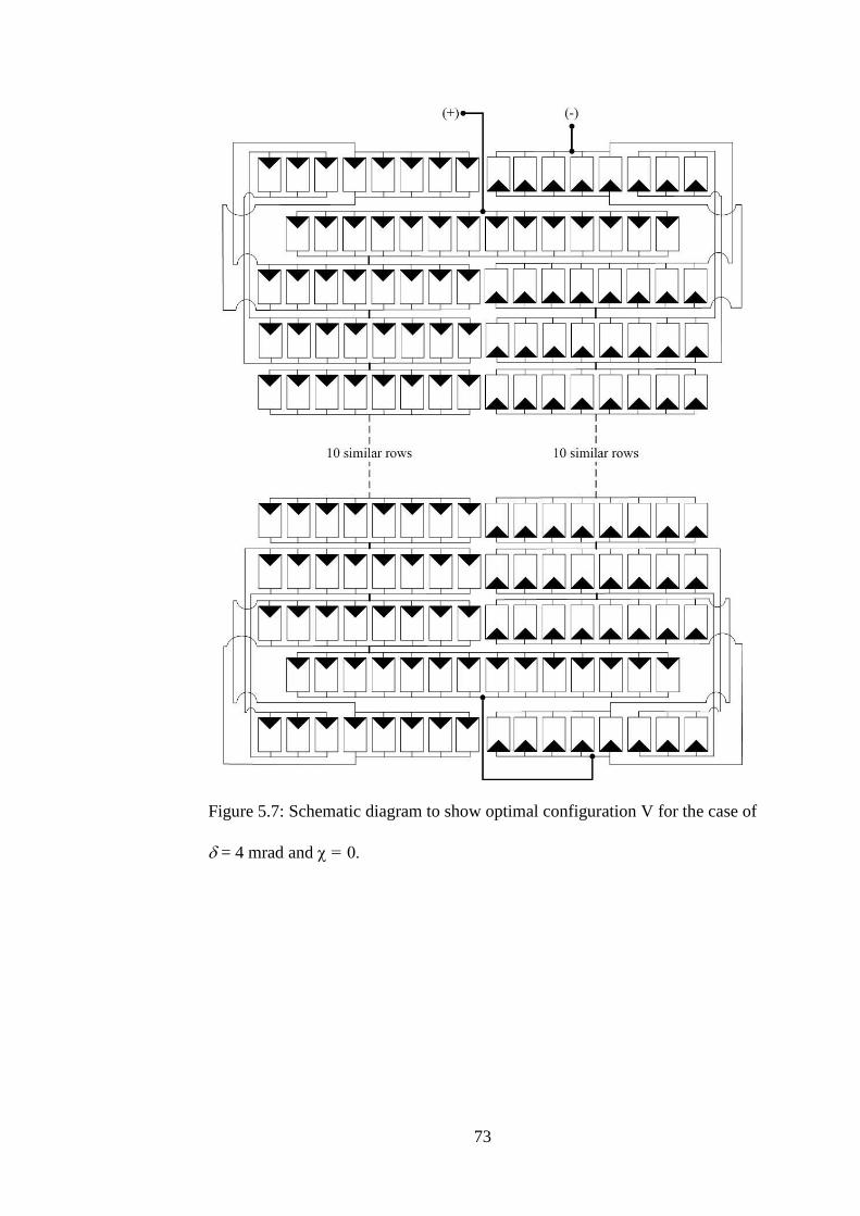
73

Figure 5.7: Schematic diagram to show optimal configuration V for the case of

= 4 mrad and = 0.

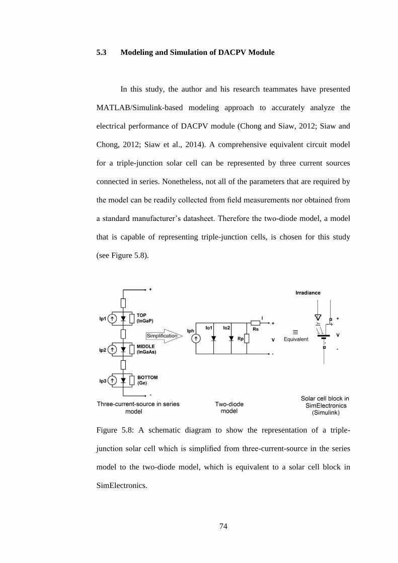
74

5.3 Modeling and Simulation of DACPV Module

In this study, the author and his research teammates have presented

MATLAB/Simulink-based modeling approach to accurately analyze the

electrical performance of DACPV module (Chong and Siaw, 2012; Siaw and

Chong, 2012; Siaw et al., 2014). A comprehensive equivalent circuit model

for a triple-junction solar cell can be represented by three current sources

connected in series. Nonetheless, not all of the parameters that are required by

the model can be readily collected from field measurements nor obtained from

a standard manufacturer’s datasheet. Therefore the two-diode model, a model

that is capable of representing triple-junction cells, is chosen for this study

(see Figure 5.8).

Figure 5.8: A schematic diagram to show the representation of a triple-

junction solar cell which is simplified from three-current-source in the series

model to the two-diode model, which is equivalent to a solar cell block in

SimElectronics.

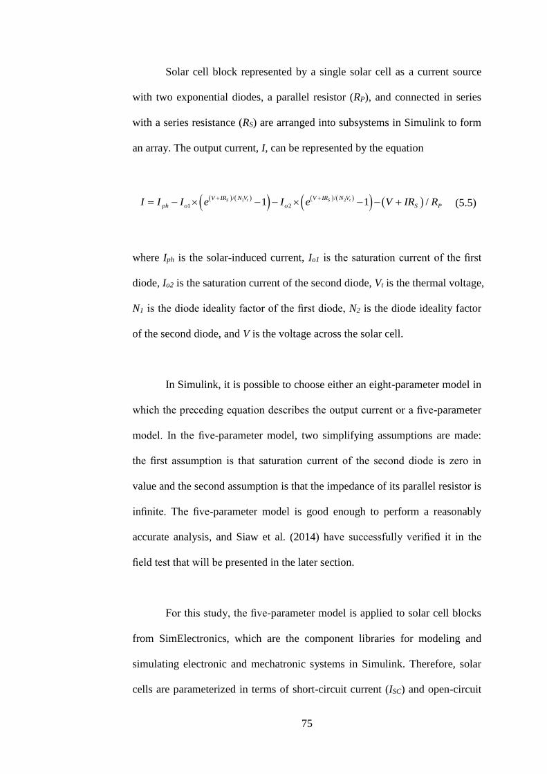
75

Solar cell block represented by a single solar cell as a current source

with two exponential diodes, a parallel resistor (RP), and connected in series

with a series resistance (RS) are arranged into subsystems in Simulink to form

an array. The output current, I, can be represented by the equation

1 2/ /

1 21 1 /S t S tV IR N V V IR N V

ph o o S PI I I e I e V IR R

(5.5)

where Iph is the solar-induced current, Io1 is the saturation current of the first

diode, Io2 is the saturation current of the second diode, Vt is the thermal voltage,

N1 is the diode ideality factor of the first diode, N2 is the diode ideality factor

of the second diode, and V is the voltage across the solar cell.

In Simulink, it is possible to choose either an eight-parameter model in

which the preceding equation describes the output current or a five-parameter

model. In the five-parameter model, two simplifying assumptions are made:

the first assumption is that saturation current of the second diode is zero in

value and the second assumption is that the impedance of its parallel resistor is

infinite. The five-parameter model is good enough to perform a reasonably

accurate analysis, and Siaw et al. (2014) have successfully verified it in the

field test that will be presented in the later section.

For this study, the five-parameter model is applied to solar cell blocks

from SimElectronics, which are the component libraries for modeling and

simulating electronic and mechatronic systems in Simulink. Therefore, solar

cells are parameterized in terms of short-circuit current (ISC) and open-circuit

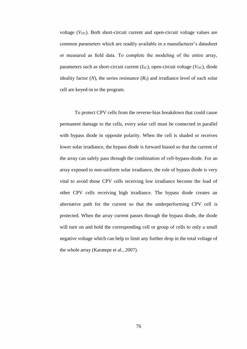
76

voltage (VOC). Both short-circuit current and open-circuit voltage values are

common parameters which are readily available in a manufacturer’s datasheet

or measured as field data. To complete the modeling of the entire array,

parameters such as short-circuit current (ISC), open-circuit voltage (VOC), diode

ideality factor (N), the series resistance (RS) and irradiance level of each solar

cell are keyed-in to the program.

To protect CPV cells from the reverse-bias breakdown that could cause

permanent damage to the cells, every solar cell must be connected in parallel

with bypass diode in opposite polarity. When the cell is shaded or receives

lower solar irradiance, the bypass diode is forward biased so that the current of

the array can safely pass through the combination of cell-bypass-diode. For an

array exposed to non-uniform solar irradiance, the role of bypass diode is very

vital to avoid those CPV cells receiving low irradiance become the load of

other CPV cells receiving high irradiance. The bypass diode creates an

alternative path for the current so that the underperforming CPV cell is

protected. When the array current passes through the bypass diode, the diode

will turn on and hold the corresponding cell or group of cells to only a small

negative voltage which can help to limit any further drop in the total voltage of

the whole array (Karatepe et al., 2007).

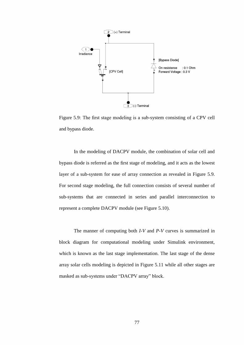
77

Figure 5.9: The first stage modeling is a sub-system consisting of a CPV cell

and bypass diode.

In the modeling of DACPV module, the combination of solar cell and

bypass diode is referred as the first stage of modeling, and it acts as the lowest

layer of a sub-system for ease of array connection as revealed in Figure 5.9.

For second stage modeling, the full connection consists of several number of

sub-systems that are connected in series and parallel interconnection to

represent a complete DACPV module (see Figure 5.10).

The manner of computing both I-V and P-V curves is summarized in

block diagram for computational modeling under Simulink environment,

which is known as the last stage implementation. The last stage of the dense

array solar cells modeling is depicted in Figure 5.11 while all other stages are

masked as sub-systems under “DACPV array” block.

78

Figure 5.10: The second stage modeling is a Simulink sub-system assembly.

In this example, 12 4 solar cells are connected using Series-Parallel

configuration to form a DACPV module (Siaw et al., 2014).

Figure 5.11: Overall Simulink implementation of DACPV module simulation

with block diagram.

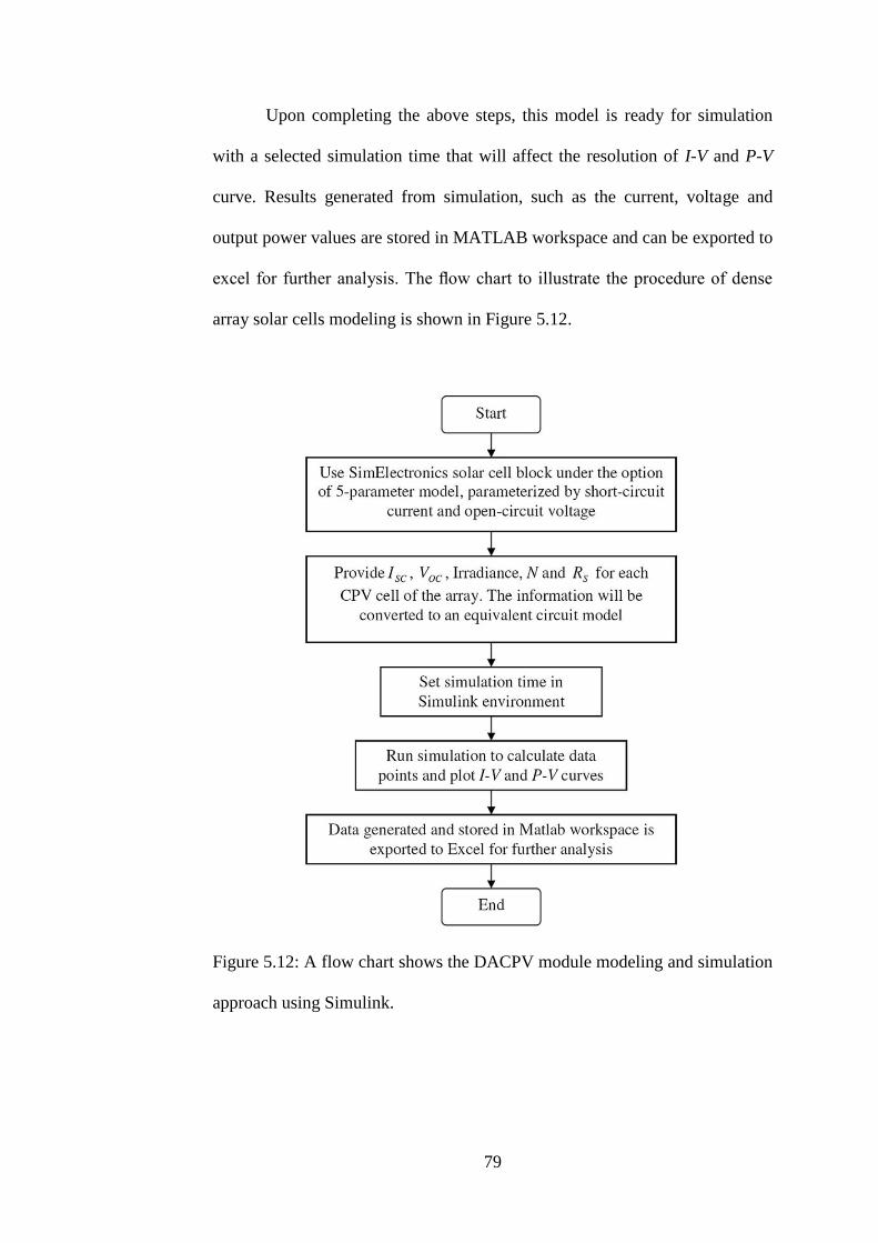
79

Upon completing the above steps, this model is ready for simulation

with a selected simulation time that will affect the resolution of I-V and P-V

curve. Results generated from simulation, such as the current, voltage and

output power values are stored in MATLAB workspace and can be exported to

excel for further analysis. The flow chart to illustrate the procedure of dense

array solar cells modeling is shown in Figure 5.12.

Figure 5.12: A flow chart shows the DACPV module modeling and simulation

approach using Simulink.

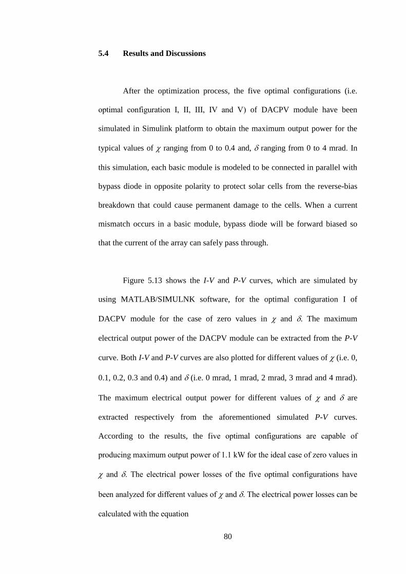
80


After the optimization process, the five optimal configurations (i.e.

optimal configuration I, II, III, IV and V) of DACPV module have been

simulated in Simulink platform to obtain the maximum output power for the

typical values of ranging from 0 to 0.4 and, ranging from 0 to 4 mrad. In

this simulation, each basic module is modeled to be connected in parallel with

bypass diode in opposite polarity to protect solar cells from the reverse-bias

breakdown that could cause permanent damage to the cells. When a current

mismatch occurs in a basic module, bypass diode will be forward biased so

that the current of the array can safely pass through.

Figure 5.13 shows the I-V and P-V curves, which are simulated by

using MATLAB/SIMULNK software, for the optimal configuration I of

DACPV module for the case of zero values in and . The maximum

electrical output power of the DACPV module can be extracted from the P-V

curve. Both I-V and P-V curves are also plotted for different values of (i.e. 0,

0.1, 0.2, 0.3 and 0.4) and (i.e. 0 mrad, 1 mrad, 2 mrad, 3 mrad and 4 mrad).

The maximum electrical output power for different values of and are

extracted respectively from the aforementioned simulated P-V curves.

According to the results, the five optimal configurations are capable of

producing maximum output power of 1.1 kW for the ideal case of zero values in

and . The electrical power losses of the five optimal configurations have

been analyzed for different values of and . The electrical power losses can be

calculated with the equation

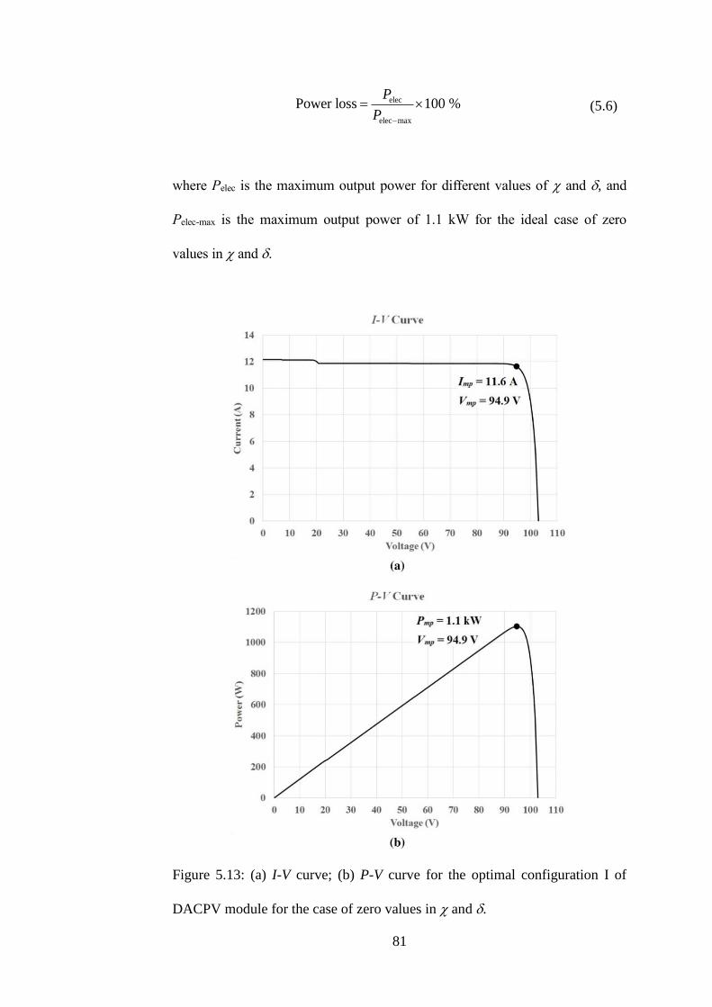
81

elec

elec max

Power loss 100 %P

P

(5.6)

where Pelec is the maximum output power for different values of and , and

Pelec-max is the maximum output power of 1.1 kW for the ideal case of zero

values in and .

Figure 5.13: (a) I-V curve; (b) P-V curve for the optimal configuration I of

DACPV module for the case of zero values in and .

82

The electrical power losses of the optimal configuration I, II, III, IV and

V for the values of , ranging from 0 to 0.4 and , ranging from 0 to 4 mrad are

shown in Figure 5.14 to 5.18, respectively. By comparing the results shown in

Figure 5.14 to 5.18, the optimal configuration I has the highest electrical power

losses and the optimal configuration V has the lowest electrical power losses for

all values of and as compared to the others configurations. This indicates

that a significant performance drop will happen to the configuration of DACPV

that is designed without considering the effect of slope error. The higher the

slope error, the higher the power loss will be in the optimal configuration I. In

addition, when increases from 0 to 0.4, the increment of electrical power

losses of optimal configuration IV and V are less significant for the case of ,

ranging from 0 to 2 mrad as compared with others configurations.

Figure 5.14: Bar chart to show the power losses in percentage for optimal

configuration I with ranging from 0 to 0.4, and ranging from 0 to 4 mrad.

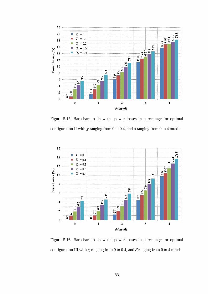
83


configuration II with ranging from 0 to 0.4, and ranging from 0 to 4 mrad.


configuration III with ranging from 0 to 0.4, and ranging from 0 to 4 mrad.

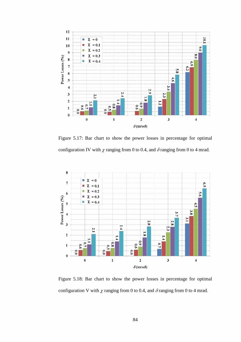
84


configuration IV with ranging from 0 to 0.4, and ranging from 0 to 4 mrad.


configuration V with ranging from 0 to 0.4, and ranging from 0 to 4 mrad.

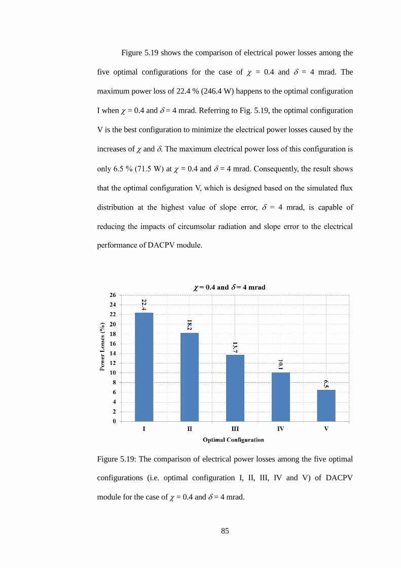
85

Figure 5.19 shows the comparison of electrical power losses among the

five optimal configurations for the case of = 0.4 and = 4 mrad. The

maximum power loss of 22.4 % (246.4 W) happens to the optimal configuration

I when = 0.4 and = 4 mrad. Referring to Fig. 5.19, the optimal configuration

V is the best configuration to minimize the electrical power losses caused by the

increases of and . The maximum electrical power loss of this configuration is

only 6.5 % (71.5 W) at = 0.4 and = 4 mrad. Consequently, the result shows

that the optimal configuration V, which is designed based on the simulated flux

distribution at the highest value of slope error, = 4 mrad, is capable of

reducing the impacts of circumsolar radiation and slope error to the electrical

performance of DACPV module.

Figure 5.19: The comparison of electrical power losses among the five optimal

configurations (i.e. optimal configuration I, II, III, IV and V) of DACPV

module for the case of = 0.4 and = 4 mrad.

86

5.5 Summary

A systematic methodology to optimize the electrical performance of

DACPV system has been proposed by considering both circumsolar radiation

() and mirror slope error (). Based on the simulated solar flux distribution,

optimal electrical interconnection of solar cells in DACVP module can be

designed by minimizing the current mismatch caused by non-uniformity of

concentrated sunlight. The optimal configuration I, II, III, IV and V are the

most optimized layout of solar cells interconnection circuits for the mirror

slope error () at 0, 1 mrad, 2 mrad, 3 mrad and 4 mrad respectively in the

case of = 0. The optimal configuration V is the best configuration for the

typical values of in the range from 0 to 4 mrad, and in the range from 0 to

0.4. The maximum electrical power loss of this configuration is only 6.5 %

(71.5 W) as compared to the ideal case (zero values in and ) that produces a

maximum output power of 1.1 kW. As a result, the optimal configuration V is

capable of reducing the impacts of circumsolar radiation and mirror slope

error to the electrical performance of DACPV module.

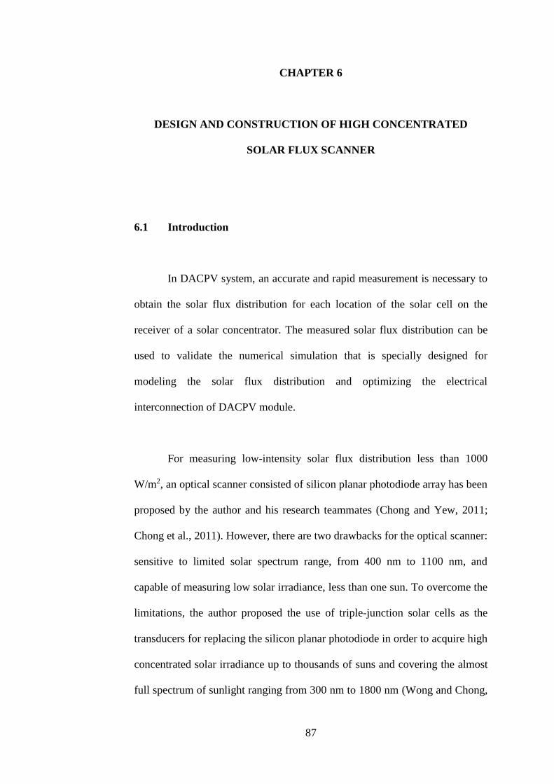
87

CHAPTER 6

DESIGN AND CONSTRUCTION OF HIGH CONCENTRATED

SOLAR FLUX SCANNER

6.1 Introduction

In DACPV system, an accurate and rapid measurement is necessary to

obtain the solar flux distribution for each location of the solar cell on the

receiver of a solar concentrator. The measured solar flux distribution can be

used to validate the numerical simulation that is specially designed for

modeling the solar flux distribution and optimizing the electrical

interconnection of DACPV module.

For measuring low-intensity solar flux distribution less than 1000

W/m2, an optical scanner consisted of silicon planar photodiode array has been

proposed by the author and his research teammates (Chong and Yew, 2011;

Chong et al., 2011). However, there are two drawbacks for the optical scanner:

sensitive to limited solar spectrum range, from 400 nm to 1100 nm, and

capable of measuring low solar irradiance, less than one sun. To overcome the

limitations, the author proposed the use of triple-junction solar cells as the

transducers for replacing the silicon planar photodiode in order to acquire high

concentrated solar irradiance up to thousands of suns and covering the almost

full spectrum of sunlight ranging from 300 nm to 1800 nm (Wong and Chong,

88

2016). Since the transducer used in the solar flux scanning device is the same

type of solar cell to be assembled in the DACPV module, it is a perfect match

for the characterization study of any new solar concentrator.

6.2 High Concentrated Solar Flux Scanner

A high concentrated solar flux scanner, also known as a flux mapping

system, has been designed and constructed to acquire flux distribution profile

of a solar concentrator. The profile is determined by measuring the short-

circuit currents of the calibrated triple-junction solar cells. The advantage of

this technique is that the triple-junction solar cell as transducer mounted on the

scanner is the same type as that of assembled in the DACPV module. It has

simplified post-processing layout design of the solar cell interconnection

circuit in the DACPV module because the short-circuit currents of solar cells

in their particular locations on the receiver have been measured directly via the

scanner. Figure 6.1 illustrates the major components needed to construct the

scanner, including an array of solar cells, relay module, current sensors,

amplifier, microcontroller, stepper motor and computer. This system is

controlled by a computer with a custom designed user interface program. It is

capable of sending commands to the microcontroller to perform desired

functions, such as to collect and to process the results of measurements.

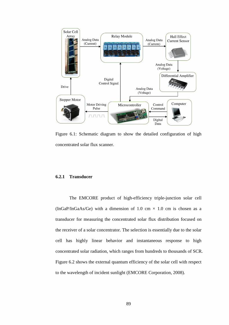
89

Figure 6.1: Schematic diagram to show the detailed configuration of high

concentrated solar flux scanner.

6.2.1 Transducer

The EMCORE product of high-efficiency triple-junction solar cell

(InGaP/InGaAs/Ge) with a dimension of 1.0 cm × 1.0 cm is chosen as a

transducer for measuring the concentrated solar flux distribution focused on

the receiver of a solar concentrator. The selection is essentially due to the solar

cell has highly linear behavior and instantaneous response to high

concentrated solar radiation, which ranges from hundreds to thousands of SCR.

Figure 6.2 shows the external quantum efficiency of the solar cell with respect

to the wavelength of incident sunlight (EMCORE Corporation, 2008).

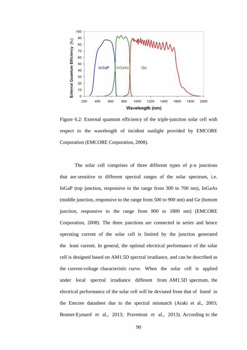
90

Figure 6.2: External quantum efficiency of the triple-junction solar cell with

respect to the wavelength of incident sunlight provided by EMCORE

Corporation (EMCORE Corporation, 2008).

The solar cell comprises of three different types of p-n junctions

that are sensitive to different spectral ranges of the solar spectrum, i.e.

InGaP (top junction, responsive to the range from 300 to 700 nm), InGaAs

(middle junction, responsive to the range from 500 to 900 nm) and Ge (bottom

junction, responsive to the range from 800 to 1800 nm) (EMCORE

Corporation, 2008). The three junctions are connected in series and hence

operating current of the solar cell is limited by the junction generated

the least current. In general, the optimal electrical performance of the solar

cell is designed based on AM1.5D spectral irradiance, and can be described as

the current-voltage characteristic curve. When the solar cell is applied

under local spectral irradiance different from AM1.5D spectrum, the

electrical performance of the solar cell will be deviated from that of listed in

the Emcore datasheet due to the spectral mismatch (Araki et al., 2003;

Bonnet-Eymard et al., 2013; Pravettoni et al., 2013). According to the

91

datasheet by the manufacturer, current measurement demonstrates far better

linearity than voltage measurement under different SCR (EMCORE

Corporation, 2008). The short-circuit current produced by the solar cell

increases linearly with SCR from one sun to as high as 1182 suns and thus the

solar flux map on the receiver can be determined by purely measuring the

short-circuit current of the solar cell.

6.2.2 Hardware Design

Instead of using a two-dimensional array of solar cells, the high solar

flux scanner consists of twenty solar cells that are arranged in a linear array.

The linear array of solar cells measures the solar flux map across a receiver

plane in a direction from left to right. This linear scanning technique can

significantly cut down the cost and complexity of the acquisition system for

solar flux map with much less number of solar cells required. With a linear

array, it is possible to have the arrangement of the solar cells with very

minimum gap spacing between the adjacent cells that will affect the resolution

of the solar flux distribution map. The resolution of the scanner is 1.0 cm × 1.2

cm equal to the dimension of the solar cell (1 cm × 1 cm) plus the gap spacing

between the adjacent cells (1.0 cm × 0.2 cm) along the column direction.

Prior to the assembling of solar flux scanner, the electrical

characteristics of solar cells must be investigated with the application of the

semiconductor parameter analyzer to ensure all of the solar cells have almost

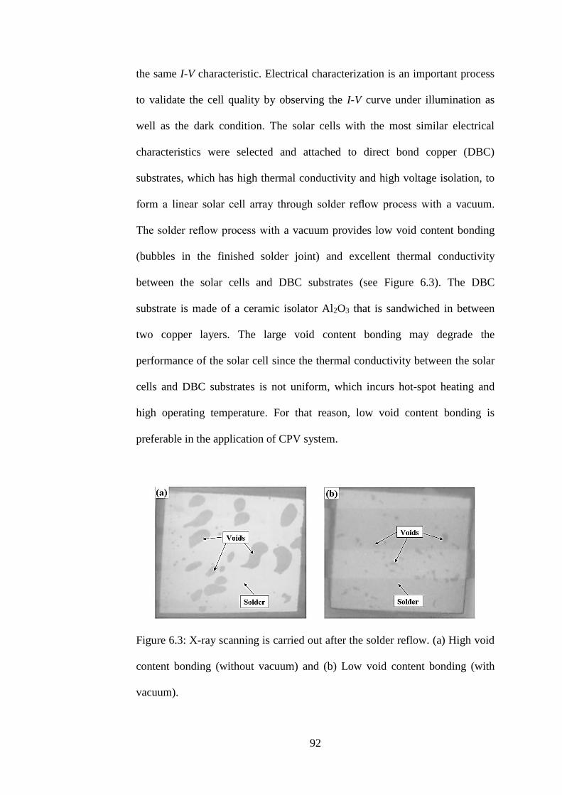
92

the same I-V characteristic. Electrical characterization is an important process

to validate the cell quality by observing the I-V curve under illumination as

well as the dark condition. The solar cells with the most similar electrical

characteristics were selected and attached to direct bond copper (DBC)

substrates, which has high thermal conductivity and high voltage isolation, to

form a linear solar cell array through solder reflow process with a vacuum.

The solder reflow process with a vacuum provides low void content bonding

(bubbles in the finished solder joint) and excellent thermal conductivity

between the solar cells and DBC substrates (see Figure 6.3). The DBC

substrate is made of a ceramic isolator Al2O3 that is sandwiched in between

two copper layers. The large void content bonding may degrade the

performance of the solar cell since the thermal conductivity between the solar

cells and DBC substrates is not uniform, which incurs hot-spot heating and

high operating temperature. For that reason, low void content bonding is

preferable in the application of CPV system.

Figure 6.3: X-ray scanning is carried out after the solder reflow. (a) High void

content bonding (without vacuum) and (b) Low void content bonding (with

vacuum).

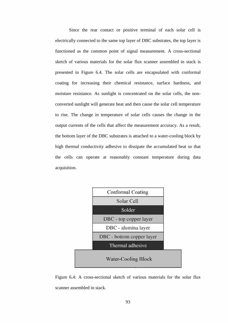
93

Since the rear contact or positive terminal of each solar cell is

electrically connected to the same top layer of DBC substrates, the top layer is

functioned as the common point of signal measurement. A cross-sectional

sketch of various materials for the solar flux scanner assembled in stack is

presented in Figure 6.4. The solar cells are encapsulated with conformal

coating for increasing their chemical resistance, surface hardness, and

moisture resistance. As sunlight is concentrated on the solar cells, the non-

converted sunlight will generate heat and then cause the solar cell temperature

to rise. The change in temperature of solar cells causes the change in the

output currents of the cells that affect the measurement accuracy. As a result,

the bottom layer of the DBC substrates is attached to a water-cooling block by

high thermal conductivity adhesive to dissipate the accumulated heat so that

the cells can operate at reasonably constant temperature during data

acquisition.

Figure 6.4: A cross-sectional sketch of various materials for the solar flux

scanner assembled in stack.

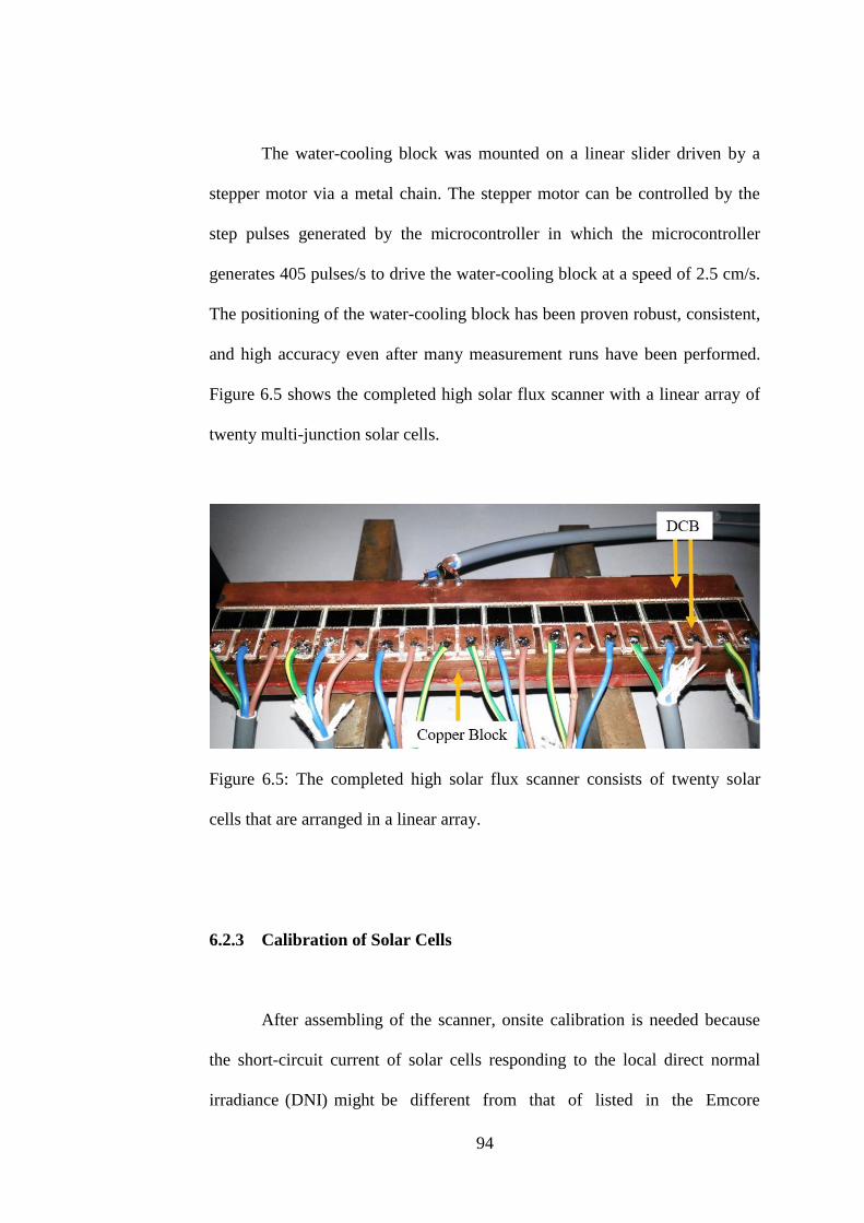
94

The water-cooling block was mounted on a linear slider driven by a

stepper motor via a metal chain. The stepper motor can be controlled by the

step pulses generated by the microcontroller in which the microcontroller

generates 405 pulses/s to drive the water-cooling block at a speed of 2.5 cm/s.

The positioning of the water-cooling block has been proven robust, consistent,

and high accuracy even after many measurement runs have been performed.

Figure 6.5 shows the completed high solar flux scanner with a linear array of

twenty multi-junction solar cells.

Figure 6.5: The completed high solar flux scanner consists of twenty solar

cells that are arranged in a linear array.

6.2.3 Calibration of Solar Cells

After assembling of the scanner, onsite calibration is needed because

the short-circuit current of solar cells responding to the local direct normal

irradiance (DNI) might be different from that of listed in the Emcore

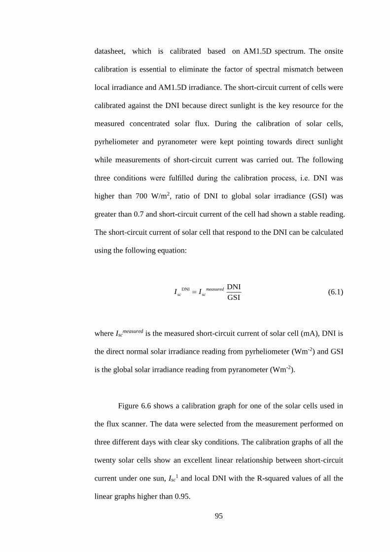
95

datasheet, which is calibrated based on AM1.5D spectrum. The onsite

calibration is essential to eliminate the factor of spectral mismatch between

local irradiance and AM1.5D irradiance. The short-circuit current of cells were

calibrated against the DNI because direct sunlight is the key resource for the

measured concentrated solar flux. During the calibration of solar cells,

pyrheliometer and pyranometer were kept pointing towards direct sunlight

while measurements of short-circuit current was carried out. The following

three conditions were fulfilled during the calibration process, i.e. DNI was

higher than 700 W/m2, ratio of DNI to global solar irradiance (GSI) was

greater than 0.7 and short-circuit current of the cell had shown a stable reading.

The short-circuit current of solar cell that respond to the DNI can be calculated

using the following equation:

DNI DNI

GSI

measured

sc scI I (6.1)

where Iscmeasured is the measured short-circuit current of solar cell (mA), DNI is

the direct normal solar irradiance reading from pyrheliometer (Wm-2) and GSI

is the global solar irradiance reading from pyranometer (Wm-2).

Figure 6.6 shows a calibration graph for one of the solar cells used in

the flux scanner. The data were selected from the measurement performed on

three different days with clear sky conditions. The calibration graphs of all the

twenty solar cells show an excellent linear relationship between short-circuit

current under one sun, Isc1 and local DNI with the R-squared values of all the

linear graphs higher than 0.95.

96

Figure 6.6: Calibration graph for one of the solar cells used in the high solar

flux scanner. The calibration graphs of all the twenty solar cells show an

excellent linear relationship between short-circuit current under one sun, Isc1

and DNI with R2 values of all the linear graphs higher than 0.95.

Regression analysis of the graphs was carried out to study the

standard error of the regression lines for all the solar cells. The standard

errors of all regression lines were calculated, and the errors were in the range

between 0.19 mA and 0.20 mA. The standard errors of all regression lines

provide simple measures of uncertainty in the calibrated short-circuit

current of the solar cells. The standard errors can be caused by the

uncertainties in irradiance (GSI and DNI) and current measurements as well as

variation of local spectral irradiance.

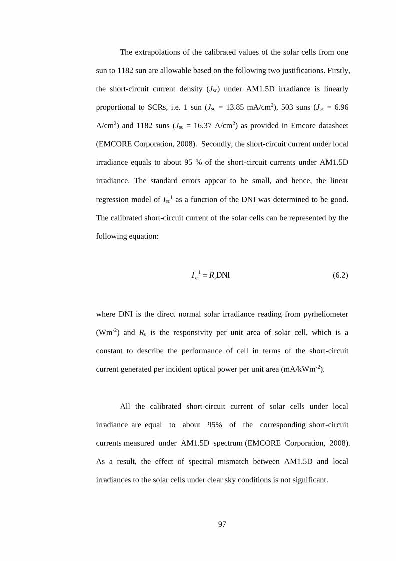
97

The extrapolations of the calibrated values of the solar cells from one

sun to 1182 sun are allowable based on the following two justifications. Firstly,

the short-circuit current density (Jsc) under AM1.5D irradiance is linearly

proportional to SCRs, i.e. 1 sun (Jsc = 13.85 mA/cm2), 503 suns (Jsc = 6.96

A/cm2) and 1182 suns (Jsc = 16.37 A/cm2) as provided in Emcore datasheet

(EMCORE Corporation, 2008). Secondly, the short-circuit current under local

irradiance equals to about 95 % of the short-circuit currents under AM1.5D

irradiance. The standard errors appear to be small, and hence, the linear

regression model of Isc1 as a function of the DNI was determined to be good.

The calibrated short-circuit current of the solar cells can be represented by the

following equation:

1 DNIsc eI R (6.2)

where DNI is the direct normal solar irradiance reading from pyrheliometer

(Wm-2) and Re is the responsivity per unit area of solar cell, which is a

constant to describe the performance of cell in terms of the short-circuit

current generated per incident optical power per unit area (mA/kWm-2).

All the calibrated short-circuit current of solar cells under local

irradiance are equal to about 95% of the corresponding short-circuit

currents measured under AM1.5D spectrum (EMCORE Corporation, 2008).

As a result, the effect of spectral mismatch between AM1.5D and local

irradiances to the solar cells under clear sky conditions is not significant.

98

6.2.4 Signal Conditioning

For the solar flux distribution measurement, signal conditioning is

necessary to convert the short-circuit current generated by the solar cell into a

voltage that is required by the data acquisition (DAQ) device for digital data

processing in a computer. The signal conditioning provides enhancement to

both the performance and accuracy of DAQ device.

The three most common sensors to sense DC current are the resistive

shunt, transimpedance amplifier, and Hall effect-based current sensor. The

resistive shunt is simply a resistor placed in series with the solar cell.

According to Ohm's law, the cell current can be determined by measuring the

voltage drop across the known resistance. This technique offers the lowest cost

and most accurate solution, but it is not suitable to be implemented for high

current measurement. Resistive power dissipation that causes a heating effect

becomes significant when a high current flows through the shunt resistor. This

may induce an erroneous reading, and the resistor will rapidly deteriorate if it

is operated near rated power without proper heat sinking. The transimpedance

amplifier is a current-to-voltage converter. It is used to convert the current

output of the sensor to a usable voltage by using an operational amplifier. The

transimpedance amplifier presents a low impedance to the current sensor, and

the output of the operational amplifier is isolated from the source. However, it

is not suitable to be employed for designing the concentrated solar flux

distribution measurement that is composed of a high input current. This is

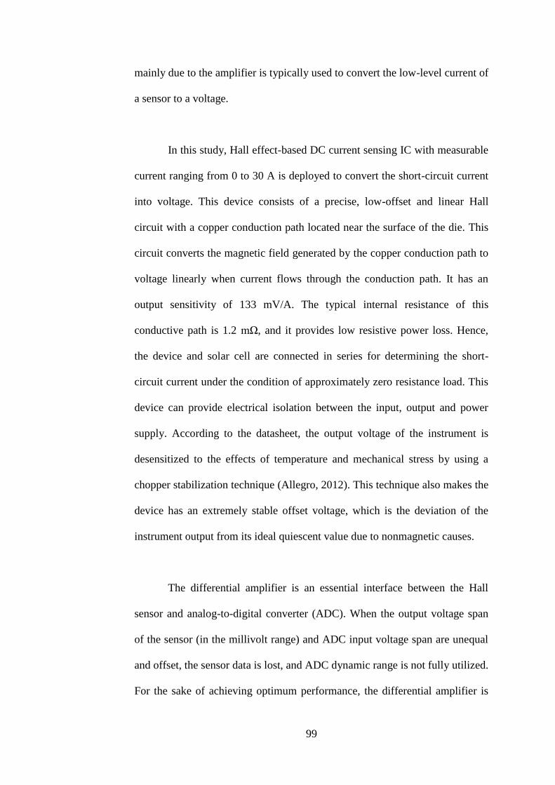
99

mainly due to the amplifier is typically used to convert the low-level current of

a sensor to a voltage.

In this study, Hall effect-based DC current sensing IC with measurable

current ranging from 0 to 30 A is deployed to convert the short-circuit current

into voltage. This device consists of a precise, low-offset and linear Hall

circuit with a copper conduction path located near the surface of the die. This

circuit converts the magnetic field generated by the copper conduction path to

voltage linearly when current flows through the conduction path. It has an

output sensitivity of 133 mV/A. The typical internal resistance of this

conductive path is 1.2 mΩ, and it provides low resistive power loss. Hence,

the device and solar cell are connected in series for determining the short-

circuit current under the condition of approximately zero resistance load. This

device can provide electrical isolation between the input, output and power

supply. According to the datasheet, the output voltage of the instrument is

desensitized to the effects of temperature and mechanical stress by using a

chopper stabilization technique (Allegro, 2012). This technique also makes the

device has an extremely stable offset voltage, which is the deviation of the

instrument output from its ideal quiescent value due to nonmagnetic causes.

The differential amplifier is an essential interface between the Hall

sensor and analog-to-digital converter (ADC). When the output voltage span

of the sensor (in the millivolt range) and ADC input voltage span are unequal

and offset, the sensor data is lost, and ADC dynamic range is not fully utilized.

For the sake of achieving optimum performance, the differential amplifier is

100

used to shift and amplify the voltage span of the sensor to match the ADC

voltage span ranging from 0 V to 5 V. A standalone Hall sensor with no input

current is functioned as a reference sensor to provide the offset voltage for the

amplifier. In addition to the offset voltage, the reference sensor is used to

minimize the noise that is caused by the magnetic field from its surroundings.

The amplifier can eliminate the error by shifting the noise voltage provided by

the reference sensor.

After the voltage level shifting and amplification, the amplified voltage

has to be converted to digital data via a microcontroller integrated with 13

channels of built-in 10-bit ADCs prior the data transferred to the computer.

Owing to the limited number of ADC, multiplexers are required to extend the

measurement channels of the microcontroller. An electronic circuit module

consisted of ten single pole double throw (SPDT) relays functioned as 2-to-1

multiplexers or data selectors is used to measure the short-circuit currents

from twenty solar cells. Figure 6.7 shows the schematic diagram of solar cells

and the corresponding electronic circuit.

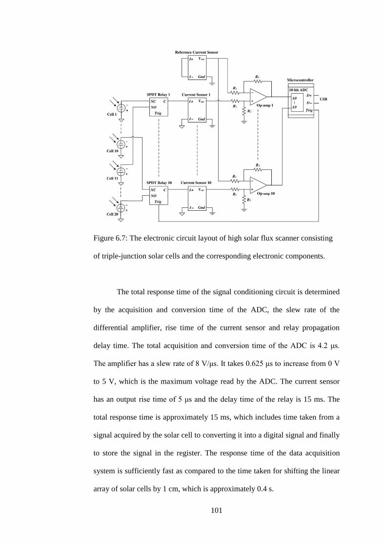
101

Figure 6.7: The electronic circuit layout of high solar flux scanner consisting

of triple-junction solar cells and the corresponding electronic components.

The total response time of the signal conditioning circuit is determined

by the acquisition and conversion time of the ADC, the slew rate of the

differential amplifier, rise time of the current sensor and relay propagation

delay time. The total acquisition and conversion time of the ADC is 4.2 μs.

The amplifier has a slew rate of 8 V/μs. It takes 0.625 μs to increase from 0 V

to 5 V, which is the maximum voltage read by the ADC. The current sensor

has an output rise time of 5 μs and the delay time of the relay is 15 ms. The

total response time is approximately 15 ms, which includes time taken from a

signal acquired by the solar cell to converting it into a digital signal and finally

to store the signal in the register. The response time of the data acquisition

system is sufficiently fast as compared to the time taken for shifting the linear

array of solar cells by 1 cm, which is approximately 0.4 s.

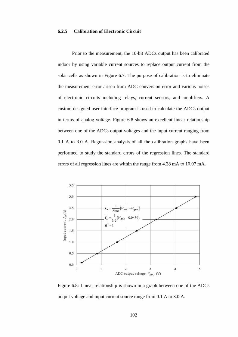
102

6.2.5 Calibration of Electronic Circuit

Prior to the measurement, the 10-bit ADCs output has been calibrated

indoor by using variable current sources to replace output current from the

solar cells as shown in Figure 6.7. The purpose of calibration is to eliminate

the measurement error arisen from ADC conversion error and various noises

of electronic circuits including relays, current sensors, and amplifiers. A

custom designed user interface program is used to calculate the ADCs output

in terms of analog voltage. Figure 6.8 shows an excellent linear relationship

between one of the ADCs output voltages and the input current ranging from

0.1 A to 3.0 A. Regression analysis of all the calibration graphs have been

performed to study the standard errors of the regression lines. The standard

errors of all regression lines are within the range from 4.38 mA to 10.07 mA.

Figure 6.8: Linear relationship is shown in a graph between one of the ADCs

output voltage and input current source range from 0.1 A to 3.0 A.

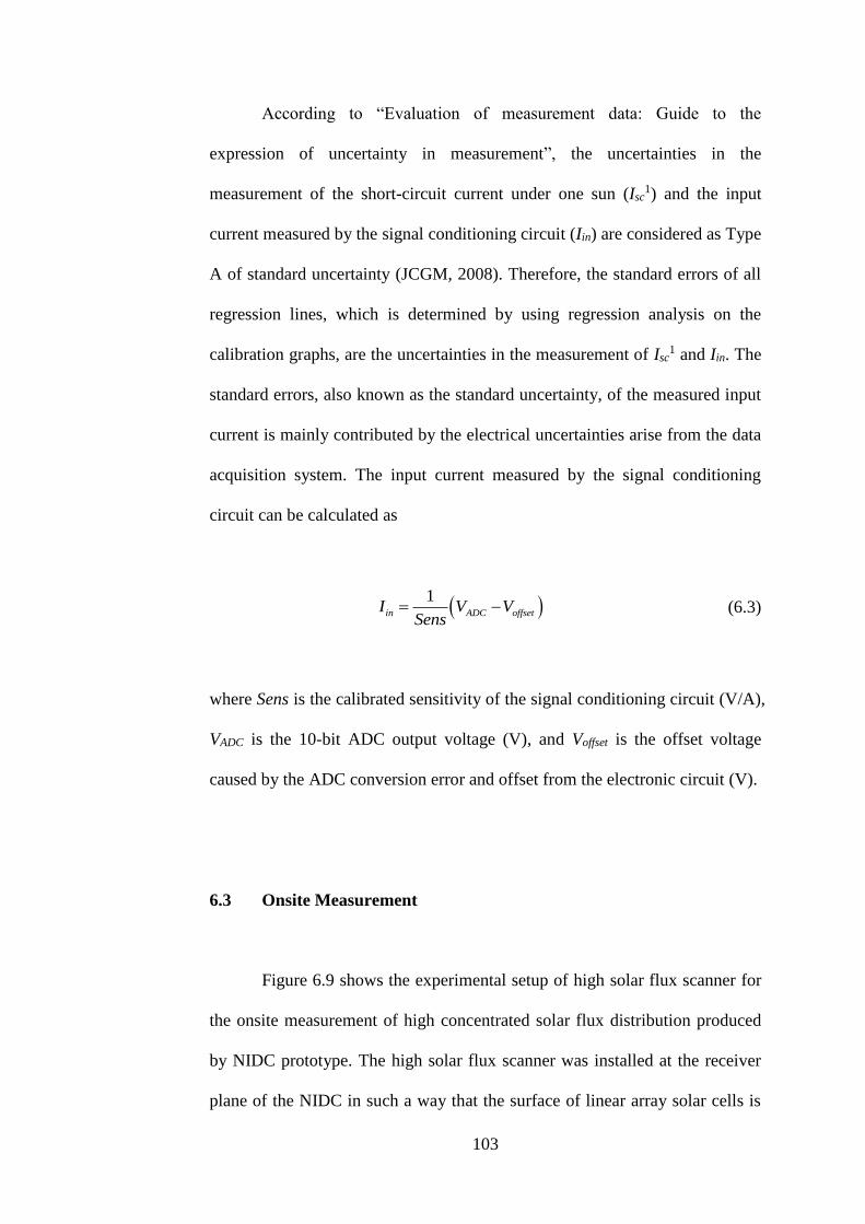
103

According to “Evaluation of measurement data: Guide to the

expression of uncertainty in measurement”, the uncertainties in the

measurement of the short-circuit current under one sun (Isc1) and the input

current measured by the signal conditioning circuit (Iin) are considered as Type

A of standard uncertainty (JCGM, 2008). Therefore, the standard errors of all

regression lines, which is determined by using regression analysis on the

calibration graphs, are the uncertainties in the measurement of Isc1 and Iin. The

standard errors, also known as the standard uncertainty, of the measured input

current is mainly contributed by the electrical uncertainties arise from the data

acquisition system. The input current measured by the signal conditioning

circuit can be calculated as

1

in ADC offsetI V VSens

(6.3)

where Sens is the calibrated sensitivity of the signal conditioning circuit (V/A),

VADC is the 10-bit ADC output voltage (V), and Voffset is the offset voltage

caused by the ADC conversion error and offset from the electronic circuit (V).

6.3 Onsite Measurement

Figure 6.9 shows the experimental setup of high solar flux scanner for

the onsite measurement of high concentrated solar flux distribution produced

by NIDC prototype. The high solar flux scanner was installed at the receiver

plane of the NIDC in such a way that the surface of linear array solar cells is

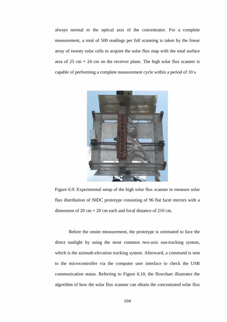
104

always normal to the optical axis of the concentrator. For a complete

measurement, a total of 500 readings per full scanning is taken by the linear

array of twenty solar cells to acquire the solar flux map with the total surface

area of 25 cm × 24 cm on the receiver plane. The high solar flux scanner is

capable of performing a complete measurement cycle within a period of 10 s.

Figure 6.9: Experimental setup of the high solar flux scanner to measure solar

flux distribution of NIDC prototype consisting of 96 flat facet mirrors with a

dimension of 20 cm × 20 cm each and focal distance of 210 cm.

Before the onsite measurement, the prototype is orientated to face the

direct sunlight by using the most common two-axis sun-tracking system,

which is the azimuth-elevation tracking system. Afterward, a command is sent

to the microcontroller via the computer user interface to check the USB

communication status. Referring to Figure 6.10, the flowchart illustrates the

algorithm of how the solar flux scanner can obtain the concentrated solar flux

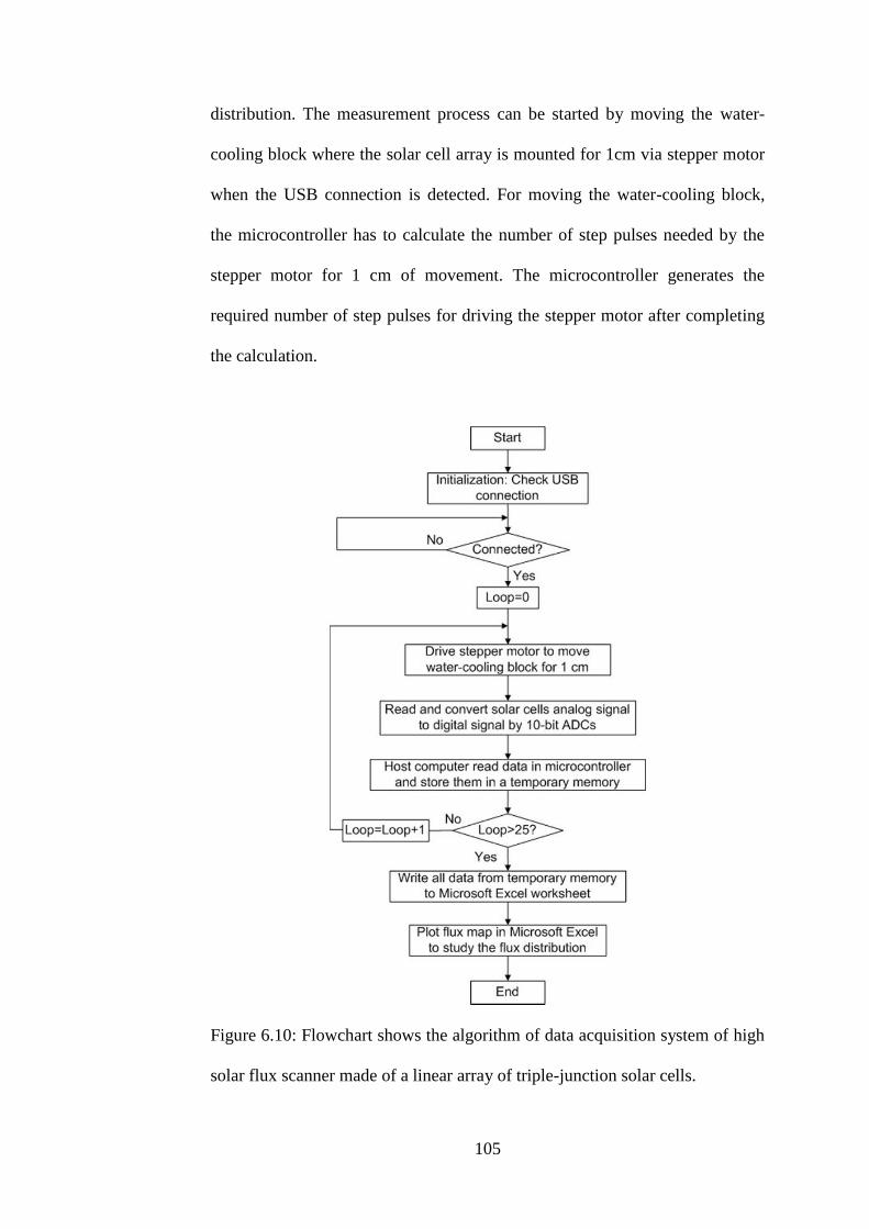
105

distribution. The measurement process can be started by moving the water-

cooling block where the solar cell array is mounted for 1cm via stepper motor

when the USB connection is detected. For moving the water-cooling block,

the microcontroller has to calculate the number of step pulses needed by the

stepper motor for 1 cm of movement. The microcontroller generates the

required number of step pulses for driving the stepper motor after completing

the calculation.

Figure 6.10: Flowchart shows the algorithm of data acquisition system of high

solar flux scanner made of a linear array of triple-junction solar cells.

106

For each centimeter of movement of the water-cooling block, the

microcontroller acquires the analog data from all the solar cells simultaneously

through the signal conditioning circuit. The analog data are converted to the

digital data via the 10-bit ADCs. The digital data are then stored in the USB

communication registers in the microcontroller. After completing the

conversion process, the host computer read the digital data in registers and

stores them in a temporary memory. This data collection process is repeated

25 times. That is equal to 25 cm in the distance of the water-cooling block has

been moved. After the measurement has completed, the data collected are

written to a Microsoft Office Excel worksheet, and the flux map is then plotted.

In this study, the flux map is represented by the measured SCR, Cmeasured and it

can be determined by the following equation:

1

1 ( 25)in cell

measured

sc

I TC

I

(6.4)

where Iin is the measured short-circuit current that is generated by the solar

cell under concentrated flux distribution, is the temperature coefficient of

short-circuit current ( = 0.065 %/ºC), Tcell is the temperature of the solar cell

during measurement in ºC, Isc1 is the calibrated short-circuit current that

responses linearly to DNI.

The high-speed scanning can reduce the problem of heat management

of the solar cell array due to the short exposure time to solar radiation. The

initial and final positions of the array are set to be off from the flux

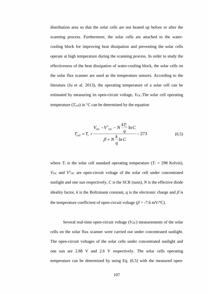
107

distribution area so that the solar cells are not heated up before or after the

scanning process. Furthermore, the solar cells are attached to the water-

cooling block for improving heat dissipation and preventing the solar cells

operate at high temperature during the scanning process. In order to study the

effectiveness of the heat dissipation of water-cooling block, the solar cells on

the solar flux scanner are used as the temperature sensors. According to the

literature (Ju et al. 2013), the operating temperature of a solar cell can be

estimated by measuring its open-circuit voltage, VOC.The solar cell operating

temperature (Tcell) in C can be determined by the equation

1 ln

273

ln

rOC OC

cell r

kTV V N C

qT T

kN C

q

(6.5)

where Tr is the solar cell standard operating temperature (Tr = 298 Kelvin),

VOC and V1OC are open-circuit voltage of the solar cell under concentrated

sunlight and one sun respectively, C is the SCR (suns), N is the effective diode

ideality factor, k is the Boltzmann constant, q is the electronic charge and is

the temperature coefficient of open-circuit voltage ( = -7.6 mV/ºC).

Several real-time open-circuit voltage (VOC) measurements of the solar

cells on the solar flux scanner were carried out under concentrated sunlight.

The open-circuit voltages of the solar cells under concentrated sunlight and

one sun are 2.88 V and 2.6 V respectively. The solar cells operating

temperature can be determined by using Eq. (6.5) with the measured open-

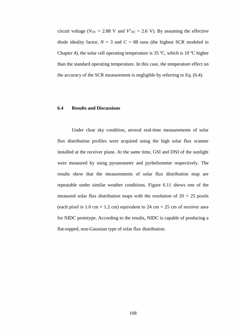
108

circuit voltage (VOC = 2.88 V and V1OC = 2.6 V). By assuming the effective

diode ideality factor, N = 3 and C = 88 suns (the highest SCR modeled in

Chapter 4), the solar cell operating temperature is 35 ºC, which is 10 ºC higher

than the standard operating temperature. In this case, the temperature effect on

the accuracy of the SCR measurement is negligible by referring to Eq. (6.4).


Under clear sky condition, several real-time measurements of solar

flux distribution profiles were acquired using the high solar flux scanner

installed at the receiver plane. At the same time, GSI and DNI of the sunlight

were measured by using pyranometer and pyrheliometer respectively. The

results show that the measurements of solar flux distribution map are

repeatable under similar weather conditions. Figure 6.11 shows one of the

measured solar flux distribution maps with the resolution of 20 × 25 pixels

(each pixel is 1.0 cm × 1.2 cm) equivalent to 24 cm × 25 cm of receiver area

for NIDC prototype. According to the results, NIDC is capable of producing a

flat-topped, non-Gaussian type of solar flux distribution.

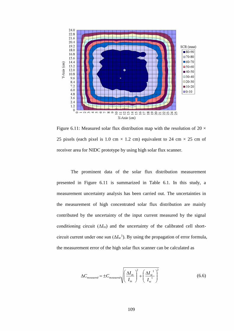
109

Figure 6.11: Measured solar flux distribution map with the resolution of 20 ×

25 pixels (each pixel is 1.0 cm × 1.2 cm) equivalent to 24 cm × 25 cm of

receiver area for NIDC prototype by using high solar flux scanner.

The prominent data of the solar flux distribution measurement

presented in Figure 6.11 is summarized in Table 6.1. In this study, a

measurement uncertainty analysis has been carried out. The uncertainties in

the measurement of high concentrated solar flux distribution are mainly

contributed by the uncertainty of the input current measured by the signal

conditioning circuit (ΔIin) and the uncertainty of the calibrated cell short-

circuit current under one sun (ΔIsc1). By using the propagation of error formula,

the measurement error of the high solar flux scanner can be calculated as

2

1

12

sc

sc

in

inmeasuredmeasured

I

I

I

ICC

(6.6)

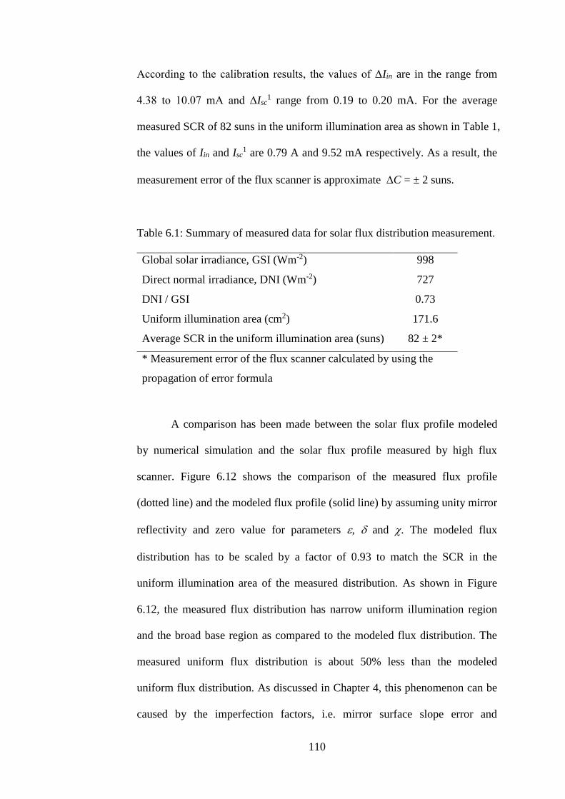
110

According to the calibration results, the values of ΔIin are in the range from

4.38 to 10.07 mA and ΔIsc1 range from 0.19 to 0.20 mA. For the average

measured SCR of 82 suns in the uniform illumination area as shown in Table 1,

the values of Iin and Isc1 are 0.79 A and 9.52 mA respectively. As a result, the

measurement error of the flux scanner is approximate C = ± 2 suns.

Table 6.1: Summary of measured data for solar flux distribution measurement.

Global solar irradiance, GSI (Wm-2) 998

Direct normal irradiance, DNI (Wm-2) 727

DNI / GSI 0.73

Uniform illumination area (cm2) 171.6

Average SCR in the uniform illumination area (suns) 82 ± 2*

* Measurement error of the flux scanner calculated by using the

propagation of error formula

A comparison has been made between the solar flux profile modeled

by numerical simulation and the solar flux profile measured by high flux

scanner. Figure 6.12 shows the comparison of the measured flux profile

(dotted line) and the modeled flux profile (solid line) by assuming unity mirror

reflectivity and zero value for parameters , and . The modeled flux

distribution has to be scaled by a factor of 0.93 to match the SCR in the

uniform illumination area of the measured distribution. As shown in Figure

6.12, the measured flux distribution has narrow uniform illumination region

and the broad base region as compared to the modeled flux distribution. The

measured uniform flux distribution is about 50% less than the modeled

uniform flux distribution. As discussed in Chapter 4, this phenomenon can be

caused by the imperfection factors, i.e. mirror surface slope error and

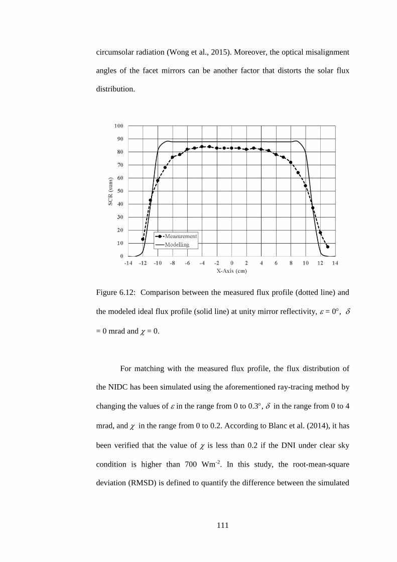
111

circumsolar radiation (Wong et al., 2015). Moreover, the optical misalignment

angles of the facet mirrors can be another factor that distorts the solar flux

distribution.

Figure 6.12: Comparison between the measured flux profile (dotted line) and

the modeled ideal flux profile (solid line) at unity mirror reflectivity, = 0,

= 0 mrad and = 0.

For matching with the measured flux profile, the flux distribution of

the NIDC has been simulated using the aforementioned ray-tracing method by

changing the values of in the range from 0 to 0.3, in the range from 0 to 4

mrad, and in the range from 0 to 0.2. According to Blanc et al. (2014), it has

been verified that the value of is less than 0.2 if the DNI under clear sky

condition is higher than 700 Wm-2. In this study, the root-mean-square

deviation (RMSD) is defined to quantify the difference between the simulated

112

SCR by ray-tracing method and the measured SCR by high flux scanner,

which is expressed as follows:

2

mod , m ,

1RMSD

T

eled t easured t

t

C C

T

(6.7)

where T is the total number of readings.

Referring to Figure 6.13, the flowchart illustrates the procedure of how

to determine the RMSD between the flux profile modeled by numerical

simulation and the flux profile measured by high flux scanner with the

application of Microsoft Office Excel. The process is started by inserting the

SCR values, Cmeasured, of measured flux map (20 × 25 pixels of readings as

shown in Figure 6.11) in 2-D matrix array into the corresponding arrangement

of 20 × 25 cells in a Microsoft Office Excel sheet. The simulated solar flux

distribution with the dimension of 24 cm × 25 cm is also sub-divided into 20 ×

25 pixels (each pixel with an area of 1.0 cm × 1.2 cm) in which average SCR

value, Cmodeled, is computed for each pixel. Subsequently, the computed SCR

values, Cmodeled, are also written into the corresponding arrangement of 20 × 25

cells of Microsoft Office Excel sheet. By mapping the value of Cmodeled to the

value of Cmeasured based on their respective positions on the receiver plane, the

RMSD is determined for each pixel by using the Eq. (6.7). The calculation is

repeated for 500 times because there is a total of 500 pixels per receiver plane

with a total surface area of 25 cm × 24 cm.

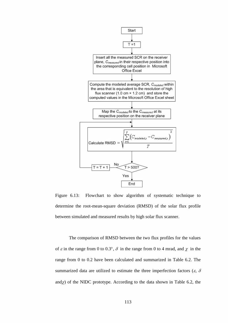
113

Figure 6.13: Flowchart to show algorithm of systematic technique to

determine the root-mean-square deviation (RMSD) of the solar flux profile

between simulated and measured results by high solar flux scanner.

The comparison of RMSD between the two flux profiles for the values

of in the range from 0 to 0.3, in the range from 0 to 4 mrad, and in the

range from 0 to 0.2 have been calculated and summarized in Table 6.2. The

summarized data are utilized to estimate the three imperfection factors (,

and) of the NIDC prototype. According to the data shown in Table 6.2, the

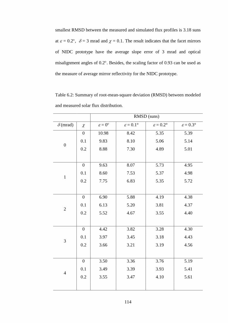
114

smallest RMSD between the measured and simulated flux profiles is 3.18 suns

at = 0.2, = 3 mrad and = 0.1. The result indicates that the facet mirrors

of NIDC prototype have the average slope error of 3 mrad and optical

misalignment angles of 0.2. Besides, the scaling factor of 0.93 can be used as

the measure of average mirror reflectivity for the NIDC prototype.

Table 6.2: Summary of root-mean-square deviation (RMSD) between modeled

and measured solar flux distribution.

RMSD (suns)

(mrad) = 0 = 0.1° = 0.2° = 0.3°

0

0 10.98 8.42 5.35 5.39

0.1 9.83 8.10 5.06 5.14

0.2 8.88 7.30 4.89 5.01

1

0 9.63 8.07 5.73 4.95

0.1 8.60 7.53 5.37 4.98

0.2 7.75 6.83 5.35 5.72

2

0 6.90 5.88 4.19 4.38

0.1 6.13 5.20 3.81 4.37

0.2 5.52 4.67 3.55 4.40

3

0 4.42 3.82 3.28 4.30

0.1 3.97 3.45 3.18 4.43

0.2 3.66 3.21 3.19 4.56

4

0 3.50 3.36 3.76 5.19

0.1 3.49 3.39 3.93 5.41

0.2 3.55 3.47 4.10 5.61

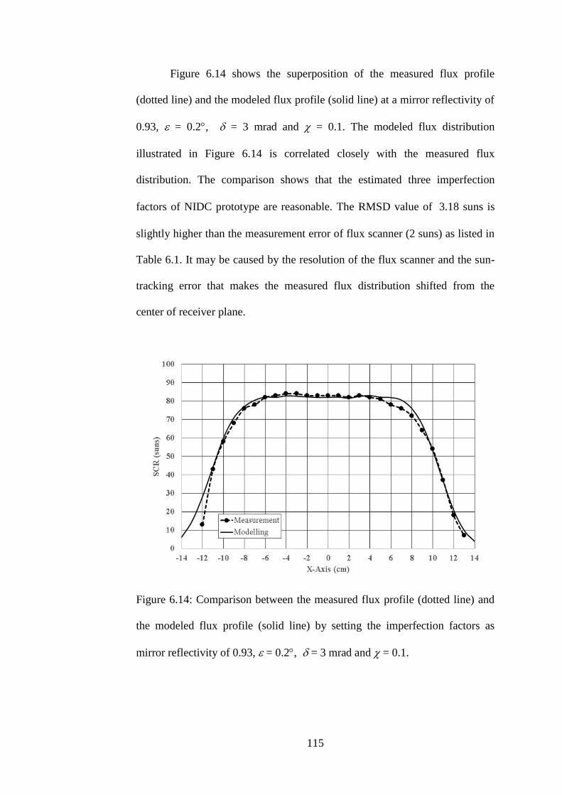
115

Figure 6.14 shows the superposition of the measured flux profile

(dotted line) and the modeled flux profile (solid line) at a mirror reflectivity of

0.93, = 0.2, = 3 mrad and = 0.1. The modeled flux distribution

illustrated in Figure 6.14 is correlated closely with the measured flux

distribution. The comparison shows that the estimated three imperfection

factors of NIDC prototype are reasonable. The RMSD value of 3.18 suns is

slightly higher than the measurement error of flux scanner (2 suns) as listed in

Table 6.1. It may be caused by the resolution of the flux scanner and the sun-

tracking error that makes the measured flux distribution shifted from the

center of receiver plane.

Figure 6.14: Comparison between the measured flux profile (dotted line) and

the modeled flux profile (solid line) by setting the imperfection factors as

mirror reflectivity of 0.93, = 0.2, = 3 mrad and = 0.1.

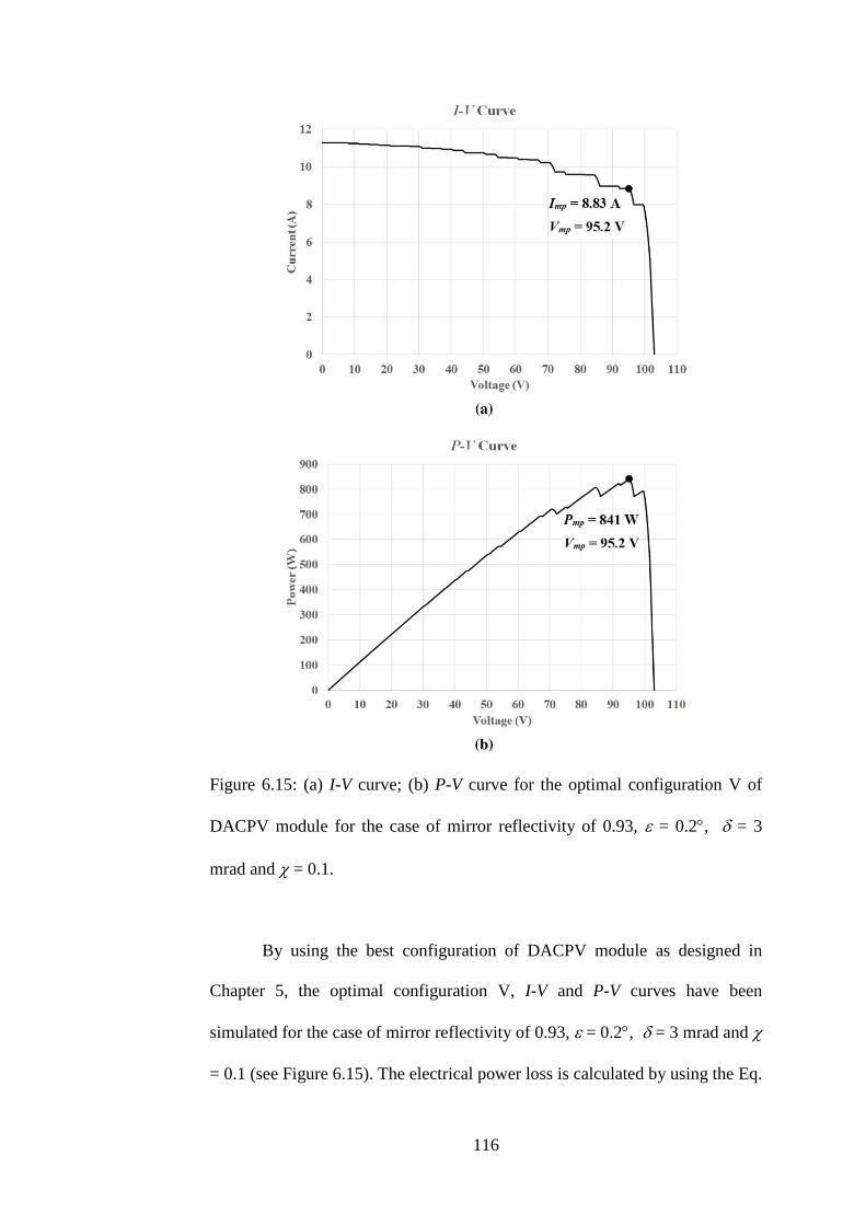
116

Figure 6.15: (a) I-V curve; (b) P-V curve for the optimal configuration V of

DACPV module for the case of mirror reflectivity of 0.93, = 0.2, = 3

mrad and = 0.1.

By using the best configuration of DACPV module as designed in

Chapter 5, the optimal configuration V, I-V and P-V curves have been

simulated for the case of mirror reflectivity of 0.93, = 0.2, = 3 mrad and

= 0.1 (see Figure 6.15). The electrical power loss is calculated by using the Eq.

117

(5.6). According to the results, the imperfection factors i.e. mirror reflectivity,

mirror surface slope error, circumsolar radiation and optical misalignment

cause a power loss of 23.6 % (260 W) as compared to the ideal case without

considering the three imperfection factors. As presented in Chapter 5, the ideal

case can produce a maximum output power of 1.1 kW.

6.5 Summary

A high solar flux scanner has been designed and constructed to acquire

solar flux distribution profile of a non-imaging dish concentrator (NIDC). The

scanner is capable of acquiring high concentrated solar flux distribution up to

1182 suns accurately and rapidly using an array of triple-junction solar cells.

A systematic technique has been proposed to analyze the amount of various

imperfection factors for the NIDC prototype by comparing the modeled and

measured solar flux distribution profiles. Based on the results, average mirror

reflectivity of 0.93, slope error of 3 mrad, circumsolar ratio of 0.1 and optical

misalignment angles of 0.2 have been obtained. By using the optimal

configuration V of DACPV module as designed in Chapter 5, the electrical

power loss of the NIDC prototype with the imperfection factors is 23.6 % (260

W) as compared to the ideal case (without considering the imperfection

factors) that produces a maximum output power of 1.1 kW. This shows that

the imperfection factors can cause serious degradation in the electrical output

power of a DACPV module.

118

CHAPTER 7

CONCLUSIONS AND FUTURE WORKS

7.1 NIDC System

The principle and the methodology of numerical simulation for

analyzing the optical characteristics of the NIDC have been described in detail.

From the simulated results, the author can conclude that the imperfection

factors, i.e., circumsolar ratio, mirror slope error and optical misalignment can

cause serious deterioration to the uniform flux distribution area and the

percentage of energy within the uniform illumination area. The influence of

the optical misalignment and slope error to the flux distribution at the receiver

is more significant compared to that of the circumsolar radiation. In addition,

the simulated results are very useful for the designer to optimize the size of the

receiver by considering the spillage losses. In this research, the receiver with a

dimension of 25 cm × 25 cm is chosen to capture more than 95% of solar

irradiance. In general, the simulated results have shown a reasonably good

uniformity of solar illumination and high SCR at the receiver plane. All the

optical characteristics have strongly recommended that the NIDC is very

suitable for the application in the DACPV system. It will be a cost-effective

alternative with a simple mechanical, structural design and relatively low

fabrication cost as compared to the other CPV systems.

119

7.2 Performance Optimization of DACPV System

A systematic approach to optimizing the electrical performance of

DACPV system has been developed by considering both the effects of

circumsolar radiation () and mirror slope error (). The methodology to

optimize the layout of solar cells interconnection circuit in DACPV module

has been proposed. The optimal configuration I, II, III, IV and V are the most

optimized layout of solar cells interconnection circuits, which are designed

based on the simulated flux distribution with slope error at 0, 1 mrad, 2 mrad,

3 mrad and 4 mrad respectively in the case of = 0. The optimal configuration

V is the best configuration to minimize the electrical power losses caused by

the increases of and . At = 0.4 and = 4 mrad, the maximum electrical

power loss of this configuration is only 6.5 % (71.5 W) as compared to the

ideal case (without considering imperfection factors) that produces a

maximum output power of 1.1 kW. With this technique, the performance of

DACPV system can be optimized for any concentrator such as a parabola, lens,

and non-imaging concentrator with the use of any standard solar cells in the

market. As a conclusion, a comprehensive study has been carried out to

optimize the electrical output power of DACPV system by considering the

circumsolar ratio and slope error in the solar flux distribution.

120

7.3 High Concentrated Solar Flux Scanner

A concentrated solar flux scanner equipped with an array of triple-

junction solar cells has been constructed to measure the solar irradiance across

a receiver plane of NIDC. The methodology and practical demonstration of the

scanner are reported in details. The flux scanner has a linear behavior and

instantaneous response to high concentrated solar radiation of thousands of

SCR. By using the calibrated triple-junction solar cells as the transducers, the

flux scanner is capable of acquiring the concentrated solar flux distribution

profile on the receiver of NIDC prototype in a short period time of 10 seconds.

The measured solar flux distribution shows deviation from a perfect uniform

distribution owing to various imperfection factors.

According to the comparison study between the modeled and measured

solar flux distribution profiles, the NIDC prototype with a peak SCR of 82

suns and an average mirror reflectivity of 0.93. Moreover, a systematic

technique has been developed to analyze imperfection factor of NIDC

prototype. By determining the root-mean-square deviation (RMSD) of the

solar flux profile between simulated and measured results, slope error of 3

mrad, the circumsolar ratio of 0.1 and optical misalignment angles of 0.2

have been obtained. As a conclusion, the flux scanner can perform real time

and direct measurement of high concentrated flux distribution profile with a

good degree of accuracy and fast scanning speed. The study is significant to

any newly constructed solar concentrator for the application of DACPV

module consisted of solar cells same type as that of the solar cells mounted on

121

the high flux scanner. Less post-processing is required to design the layout of

the solar cell interconnection circuit in the DACPV module since the short-

circuit currents of solar cells can be measured directly via the flux scanner.

7.4 Concluding Remarks and Future Works

The overall aims of this research are to develop a novel NIDC

prototype and a systematic methodology to optimize the electrical

interconnection of DACPV module for solving the non-uniform solar

illumination problem that restrains the electrical performance of solar cells.

The research objectives of theoretical and experimental study in optimizing

the electrical performance of DACPV system, as specified in Chapter 1, have

been achieved. The major outcomes of this project are the design and

development of an NIDC prototype, a new systematic method to optimize the

layout of solar cells interconnection circuit in DACPV module, and the

design and development of a high concentrated solar flux scanner. In

conclusion, this research is confirmed to be capable of improving the output of

solar cells with inhomogeneous illumination with a significant improvement in

the electrical performance of DACPV system.

122

The main future works related to this research are descripted as follows:

For the validation of the model with respect to the effects (deterioration

in solar flux distribution and output power of solar cells) of circumsolar

radiation, slope error and optical misalignment, it is desirable to

assemble a DACPV module that is designed based on the optimal

configuration V in the future.

Future work could design an accurate, inexpensive and fast approach to

align the flat facet mirrors of NIDC for eliminating the effect of optical

misalignment on the solar flux distribution.

It is also necessary to apply similar research approach on a bigger

size of NIDC in order to find the most optimized DACPV system.

123

REFERENCES

Allegro, 2012. Fully Integrated, Hall Effect-Based Linear Current Sensor IC

with 2.1 kVRMS Isolation and a Low-Resistance Current Conductor. ACS713

datasheet.

Andreev, V., Grilikhes, V., Rumyantsev, V., Timoshina, N. and Shvarts, M.,

2003. Effect of nonuniform light intensity distribution on temperature

coefficients of concentrator solar cells. 3rd World Conference on Photovoltaic

Energy Conversion, 2003, pp. 881-884.

Araki, K., and Yamaguchi, M., 2003. Influences of spectrum change to 3-

junction concentrator cells. Solar Energy Materials and Solar Cells, 75,

pp.707–714.

Baig, H., Heasman, K.C. and Mallick, T.K., 2012. Non-uniform illumination in

concentrating solar cells. Renewable and Sustainable Energy Reviews. 16 (8),

5890–5909.

Ballestrín, J. et al., 2003. Systematic error in the measurement of very high solar

irradiance. Solar Energy Materials and Solar Cells, 80, pp. 375–381.

Ballestrín, J. et al., 2004. High-heat-flux sensor calibration using calorimetry.

Metrologia, 41(4), pp.314–318.

124

Bett, A.W., Dimroth, F., and Siefer, G., 2007. Multijunction Concentrator Solar

Cells. In: Concentrator Photovoltaics. pp.67–87.

Blanc, P. et al., 2014. Direct normal irradiance related definitions and

applications: The circumsolar issue. Solar Energy, 110, pp.561–577.

Bonnet-Eymard, M. et al., 2013. Optimized short-circuit current mismatch in

multi-junction solar cells. Solar Energy Materials and Solar Cells, 117, pp.120–

125.

Buie, D., Dey, C.J., and Bosi, S., 2003a. The effective size of the solar cone for

solar concentrating systems. Solar Energy, 74(2003), pp.417–427.

Buie, D., Monger, a. G., and Dey, C.J., 2003b. Sunshape distributions for

terrestrial solar simulations. Solar Energy, 74(2003), pp.113–122.

Chong, K.K. and Wong, C.W., 2009. General formula for on-axis sun-tracking

system and its application in improving tracking accuracy of solar collector.

Solar Energy, 83, pp. 298–305.

Chong, K.K, and Wong, C.W., 2010. General Formula for On-Axis Sun-

Tracking System. In: Solar Collectors and Panels, Theory and Applications.

p.444.

125

Chong, K.K. and Yew, T.K., 2011. Novel optical scanner using photodiodes

array for two-dimensional measurement of light flux distribution. IEEE Trans.

Instrum. Meas., 60, pp. 2918–2925.

Chong, K.K. et al.,, 2009a. Integration of an on-axis general sun-tracking

formula in the algorithm of an open-loop sun-tracking system. Sensors, 9, pp.

7849–7865.

Chong, K.-K., and Siaw, F.-L., 2012. Electrical characterization of dense-array

concentrator photovoltaic system. In: 27th European Photovoltaic Solar Energy

Conference and Exhibition. pp.224–227.

Chong, K.K., Lau, S.L., Yew, T.K. and Tan, P.C.L., 2013a. Design and

development in optics of concentrator photovoltaic system. Renew. Sustain.

Energy Rev., 19, pp. 598 – 612

Chong, K.K., Siaw, F.L., Wong, C.W. and Wong, G.S., 2009b. Design and

construction of non-imaging planar concentrator for concentrator photovoltaic

system. Renewable Energy, 34, pp. 1364–1370.

Chong, K.-K., Tan, W.-C., and Wong, C.-W., 2012a. Second prototype non-

imaging planar concentrator for concentrator photovoltaic system. In: 27th

European Photovoltaic Solar Energy Conference and Exhibition. 2012 pp. 257–

259.

126

Chong, K.K., Wong, C.W., Siaw, F.L. and Yew, T.K., 2010. Optical

Characterization of Nonimaging Planar Concentrator for the Application in

Concentrator Photovoltaic System. Journal of Solar Energy Engineering, 132,

011011.

Chong, K.K., Wong, C.W., Yew, T.K. and Tan, M.H., 2012b. Solar

concentrator assembly. Malaysian Patent No. PI 2012002439 (pending).

Chong, K.K., Wong, C.W., Yew, T.K. and Tan, M.H., 2013b. Solar

concentrator assembly. U.S. Patent Application 13/901,519 (pending).

Chong, K.K., Yew, T.K., Wong, C.W. and Lau, S.L., 2011. Study of image

quality of mirror via solar flux distribution measurement using a high speed

optical scanner. Applied Optics, 50, pp. 4927–4935.

Cooper, T., Pravettoni, M., Cadruvi, M., Ambrosetti, G. and Steinfeld, A., 2013.

The effect of irradiance mismatch on a semi-dense array of triple-junction

concentrator cells. Solar Energy Materials and Solar Cells, 116, pp. 238–251.

Coventry, J.S., 2005. Performance of a concentrating photovoltaic/thermal solar

collector. Solar Energy, 78, pp. 211-222.

EMCORE Corporation, 2008. Triple-junction high efficiency solar cells for

terrestrial concentrated photovoltaic applications. EMCORE Photovoltaics

datasheet.

127

Estrada, C.A., Jaramillo, O.A., Acosta, R. and Arancibia-Bulnes, C.A., 2007.

Heat transfer analysis in a calorimeter for concentrated solar radiation

measurements. Solar Energy, 81, pp. 1306–1313.

Faiman, D., Biryukov, S., and Pearlmutter, K.K., May 2002. PETAL: A

research pathway to fossil-competitive solar electricity. 29th IEEE

Photovoltaic Specialist Conference, New Orleans, USA, pp. 1384-1387.

Fernandez-Reche, J. et al., 2008. Concentrating PV: An Alternative to

Calorimeters for Measuring High Solar Flux Densities. Journal of Solar Energy

Engineering, 130(4), p.044502.

Franklin, E.T., and Coventry, J.S., 2002. Effects of highly non-uniform

illumination distribution on electrical performance of solar cells. ANSES Solar

Conference. New Castle, Australia, pp. 1-8.

Green, M.A., Emery, K., Hishikawa, Y., Warta, W. and Dunlop, E.D., 2015.

Solar cell efficiency tables (version 46). Prog. Photovoltaics Res. Appl., 23, pp.

805 – 812.

Haueter, P., Seitz, T. and Steinfeld, A., 1999. A New High-Flux Solar Furnace

for High-Temperature Thermochemical Research. Journal of Solar Energy

Engineering, 121, pp. 77.

128

Heinloth, K. (eds.), 2006, Energy Technologies Subvolume C: Renewable

Energy, Springer, New York, pp. 242–278.

Johnston , G. and Shortis, M., 1997. Photogrammetry: an available surface

characterization tool for solar concentrators, Part II: Assessment of surfaces.

Journal of Solar Energy Engineering, 119(4), pp. 286–291.

Johnston, G., 1995. On the Analysis of Surface Error Distributions on

Concentrated Solar Collectors. Journal of Solar Energy Engineering, 117(4),

pp. 294–296

Johnston, G., Lovegrove, K., and Luzzi, A., 2003. Optical performance of

spherical reflecting elements for use with paraboloidal dish concentrators. Solar

Energy, 74(2), pp.133–140.

Joint Committee for Guides in Metrology (JCGM), 2008. Evaluation of

measurement data: Guide to the expression of uncertainty in measurement.

Ju, X., Vossier, A., Wang, Z., Dollet, A., and Flamant, G., 2013. An improved

temperature estimation method for solar cells operating at high concentrations.

Solar Energy, 93, pp. 80-89.

Karatepe, E., Boztepe, M., and Çolak, M., 2007. Development of a suitable

model for characterizing photovoltaic arrays with shaded solar cells. Solar

Energy, 81(8), pp.977–992.

129

Kaushika, N.D., and Rai, A.K., 2007. An investigation of mismatch losses in

solar photovoltaic cell networks. Energy, 32, pp.755–759.

King, R.R. et al., 2010. Band gap-voltage offset and energy production in next-

generation multijunction solar cells. Progress in Photovoltaics: Research and

Applications, 19(7), pp.6–11.

Kreske, K., 2002. Optical design of a solar flux homogenizer for concentrator

photovoltaics. Applied Optics, 41(10), p.2053.

Kurtz, S., Emery, K., 2015. Conversion efficiencies of best research solar cells

worldwide from 1976 through 2015 for various photovoltaic technologies

[Online]. Available at:

https://commons.wikimedia.org/wiki/File:PVeff(rev150806).jpg [Accessed: 8

November 2015].

Kussul, E. et al., 2008. Micro-facet solar concentrator. Int. J. Sustain. Energy,

27, pp. 61 – 71.

Liu, Y., Dai, J.M., Sun, X.G. and Yu,T.H., 2006. Factors influencing flux

distribution on focal region of parabolic concentrators. In: Proceeding of

International Symposium on Instrumentation Science and Technology, IOP

Science, pp. 59-63.

https://commons.wikimedia.org/wiki/File:PVeff(rev150806).jpg

130

Löckenhoff, R., Kubera, T., and Rasch, K.D., 2010. Water Cooled TJ Dense

Array Modules for Parabolic Dishes. Power, 6, pp.9–12.

Luque, A. L. and Andreev, V. M. (eds.), 2007, Concentrator Photovoltaics,

Springer, New York, pp. 113–132.

Luque, A., Sala, G., and Luque-Heredia, I., 2006. Photovoltaic concentration at

the onset of its commercial deployment. Progress in Photovoltaics: Research

and Applications, 14(5), pp.413–428.

Marz, T., Prahl, C., Ulmer, S., Wilbert, S., and Weber, C., 2011. Validation of

Two Optical Measurement Methods for the Qualification of the Shape Accuracy

of Mirror Panels for Concentrating Solar Systems. Journal of Solar Energy


Mills, D.R., and Morrison, G.L., 2000. Compact Linear Fresnel Reflector solar

thermal powerplants. Solar Energy, 68(3), pp.263–283.

Nishioka, K. et al., 2006. Evaluation of InGaP/InGaAs/Ge triple-junction solar

cell and optimization of solar cell’s structure focusing on series resistance for

high-efficiency concentrator photovoltaic systems. Solar Energy Materials and

Solar Cells, 90, pp. 1308–1321.

Noring, J.E., Grether, D.F. and Hunt, A.J., 1991. Circumsolar radiation data: the

Lawrence Berkeley Laboratory reduced data base” In: National Renewable

131

Energy Laboratory. NREL/TP-262-4429 [Online]. Available at:

http://rredc.nrel.gov/solar/pubs/circumsolar/title.html [Accessed: 15 December

2015].

Ota, Y., and Nishioka, K., 2012. Three-dimensional simulating of concentrator

photovoltaic modules using ray trace and equivalent circuit simulators. Solar

Energy, 86(1), pp.476–481.

Parretta, A. et al., 2007. Double-cavity radiometer for high-flux density solar

radiation measurements. Applied Optics, 46, pp. 2166–2179.

Parretta, A., Privato, C., Nenna, G., Antonini, A. and Stefancich, M., 2006.

Monitoring of concentrated radiation beam for photovoltaic and thermal solar

energy conversion applications. Applied Optics, 45, pp. 7885–7897.

Philipps, S.P., Bett, A.W., Horowitz, K. and Kurtz, S., 2015. Current Status of

Concentrator Photovoltaic (CPV) Technology [Online]. Available at:

http://www.ise.fraunhofer.de/en/publications/veroeffentlichungen-pdf-dateien-

en/studien-und-konzeptpapiere/current-status-of-concentrator-photovoltaic-

cpv-technology.pdf [Accessed: 8 December 2015].

Philipps, S.P., Dimroth, F. and Bett, A.W., 2012. High-Efficiency III-V

Multijunction Solar Cells, in Practical Handbook of Photovoltaics. pp. 417–

448.

http://www.ise.fraunhofer.de/en/publications/veroeffentlichungen-pdf-dateien-en/studien-und-konzeptpapiere/current-status-of-concentrator-photovoltaic-cpv-technology.pdf



132

Picault, D., Raison, B., Bacha, S., de la Casa, J., and Aguilera, J., 2010.

Forecasting photovoltaic array power production subject to mismatch losses.

Solar Energy, 84(7), pp.1301–1309.

Pottler, K., Lupfert, E.,, Johnston, G. and Shortis, M.R., 2005. Photogrammetry:

A Powerful Tool for Geometric Analysis of Solar Concentrators and Their

Components. Journal of Solar Energy Engineering, 127(1), pp. 94-101.

Pravettoni, M., Virtuani, A., Keller, K., Apolloni, M. and Müllejans, H., 2013.

Spectral Mismatch Effect to the Open-circuit Voltage in the Indoor

Characterization of Multi-junction Thin-film Photovoltaic Modules, in:

Conference Record of the 2013 IEEE 39th Photovoltaic Specialists Conference

(PVSC). pp. 706–711.

Reis, F., Pravettoni, M., Wemans, J., Sorasio, G. and Brito, M.C., 2013.

Modelling the effects of inhomogeneous irradiation and temperature profiles on

CPV cells behaviour. IEEE J. Photovoltaics, 5, pp. 112–122.

Ries, H., Gordon, J.M., and Lasken, M., 1997. High-flux photovoltaic solar

concentrators with kaleidoscope-based optical designs. Solar Energy, 60(1),

pp.11–16.

Röger, M. et al., 2014. Techniques to Measure Solar Flux Density Distribution

on Large-Scale Receivers. Journal of Solar Energy Engineering, 136, pp.

031013.

133

Ryu, K., Rhee, J.G., Park, K.M., and Kim, J., 2006. Concept and design of

modular Fresnel lenses for concentration solar PV system. Solar Energy,

80(12), pp.1580–1587.

Salomé, A., Chhel, F., Flamant, G., Ferrière, A. and Thiery, F., 2013. Control

of the flux distribution on a solar tower receiver using an optimized aiming point

strategy: Application to THEMIS solar tower. Solar Energy, 94, pp. 352–366.

Segev, G., and Kribus, A., 2013. Performance of CPV modules based on vertical

multi-junction cells under non-uniform illumination. Solar Energy, 88, pp.120–

128.

Segev, G., and Kribus, A., 2013. Performance of CPV modules based on vertical

multi-junction cells under non-uniform illumination. Solar Energy, 88, pp.120–

128.

Sharaf, O.Z. and Orhan, M.F., 2015. Concentrated photovoltaic thermal

(CPVT) solar collector systems: Part I — Fundamentals, design considerations

and current technologies. Renewable and Sustainable Energy Reviews. 50

(2015), 1500–1565.

Sherif, R., Cotal, H., Paredes, A., Lewandowski, A., Bingham, C. and Mehos,

M., 2003. High concentration tests of a dense PV array using GaInP/GaAs/Ge

triple-junction cells in the high flux solar furnace. 3rd World Conference on

Photovoltaic Energy Conversion, Osaka, Japan, pp. 829-832.

134

Siaw, F.L. and Chong, K.K., 2012. Temperature effects on the performance of

dense-array concentrator photovoltaic system. In: Proceedings of the IEEE

Conference on Sustainable Utilization and Development in Engineering and

Technology (IEEE, 2012), pp. 140–144.

Siaw, F.L. and Chong, K.K., 2013. A systematic method of interconnection

optimization for dense-array concentrator photovoltaic system. Sci. World J.,

2013, pp. 1-11.

Siaw, F.L., Chong, K.K. and Wong, C.W., 2014. A comprehensive study of

dense-array concentrator photovoltaic system using non-imaging planar

concentrator. Renewable Energy, 62, pp. 542–555.

Spectrolab, Inc., 2010. CPV Dense Array Solar Cells. Spectrolab, Inc.

datasheet.

Tan, M.-H., Chong, K.-K., Wong and C.-W., 2014. Optical characterization of

nonimaging dish concentrator for the application of dense-array concentrator

photovoltaic system. Applied Optics, 53, pp. 475–86.

Ulmer, S., Heller, P., and Reinalter, W., 2008. Slope Measurements of Parabolic

Dish Concentrators Using Color-Coded Targets. Journal of Solar Energy


135

Ulmer, S., Reinalter, W., Heller, P., Lupfert, E. and Martınez, D., 2002. Beam

Characterization and Improvement with a Flux Mapping System for Dish

Concentrators. Journal of Solar Energy Engineering, 124, pp. 182.

Verlinden, P.J et al., 2006. Performance and reliability of multijunction III-V

modules for concentrator dish and central receiver applications, in: Conference

Record of the 2006 IEEE 4th World Conference on Photovoltaic Energy

Conversion, WCPEC-4. pp. 592–597.

Vivar, M., Antón, I., and Sala, G., 2010. Radial CPV receiver. Progress in

Photovoltaics: Research and Applications, 18(5), pp.353–362.

Vivar, M., Morilla, C., Antón, I., and Sala, G., 2009. Si-cells radial parquet for

parabolic dish receivers. In: Proceedings of the 24th European Photovoltaic

Solar Energy Conference, Hamburg, Germany, September 2009, pp. 141–144.

Vossier, A., Chemisana, D., Flamant, G., and Dollet, A., 2012. Very high fluxes

for concentrating photovoltaics: Considerations from simple experiments and

modeling. Renewable Energy, 38(1), pp.31–39.

Wang, Z., Zhang, H., Wen, D., Zhao, W., and Zhou, Z., 2013. Characterization

of the InGaP/InGaAs/Ge triple-junction solar cell with a two-stage dish-style

concentration system. Energy Conversion and Management, 76, pp.177–184.

136

Winston, R., Minano, J. C., and Benitez, P., 2005, Non-Imaging Optics,

Elsevier, New York, pp. 1–6.

Wong, C.-W., Chong, K.-K. and Tan, M.-H., 2015. Performance optimization

of dense-array concentrator photovoltaic system considering effects of

circumsolar radiation and slope error. Optics Express, 23, pp. A841.

Wong, C.-W., and Chong, K.-K., 2016. Solar flux distribution study of non-

imaging dish concentrator using linear array of triple-junction solar cells

scanning technique Solar Energy, 125, pp. 86-98.

137

APPENDIX A

A.1 Main

clc

clear

SE = 0e-3; % Mirror Slope Error Value

CSR = 0.0001; % Circumsolar Ratio Value

AE = 0.0; % Optical Misalignment Value

tic; % Start Timer

% ========== Call function ==========

Initial()

Coordinate()

Rotate_Mirror()

% ========== Determine flux distribution ==========

data=zeros(PixSize);

for i=1:1:m

for j=1:1:n

for k=1:1:g

for l=1:1:h

SolarRay()

weight = N{i,j,k,l}(3)/total; % Get the weightage of Ray

data=data+flux*weight;

end

end

end

end

toc; % End Timer

% ========== Plot flux distribution ==========

x=[1:PixSize];

y=[1:PixSize];

[X,Y]= meshgrid(x,y);

figure()

mesh((X-(PixSize/2+0.5))*TargetSize/PixSize,(Y-

(PixSize/2+0.5))*TargetSize/PixSize,data);

138

A.2 Initial()

% ========= Input ===========

alfa_1= 0.00465; % Solar disc half angle (radian)

alfa_2= 0.0436; % Sun-shape half angle (radian)

m = 4; % No of mirrors in row

n = 24; % No of mirrors in column

MirrorSize = 20; % Mirror size (cm)

m_MirrorRes = 201; % Mirror resolution (Odd Num)

m_nR =101; % Solar disc resolution (Odd Num)

TargetSize = 40; % Target size (cm)

L = 210.0; % Target distance (cm)

PixSize = 401; % Target Pixel Size

% =========== Initialize ==========

PI = 3.1415926535897932384626433832795;

mc = (m + 1)/2; % Central mirror in row

nc = (n + 1)/2; % Central mirror in column

g = m_MirrorRes; % No of Rays along mirror in row

h = m_MirrorRes; % No of Rays along mirror in column

gc = (g - 1)/2; % Central Ray along rows

hc = (h - 1)/2; % Central Ray along columns

MirrorRes1 = MirrorSize/(g-1); % Mirror resolution in row

MirrorRes2 = MirrorSize/(h-1); % Mirror resolution in column

scale = PixSize/TargetSize; % pixel per cm

TargetRes = TargetSize/PixSize; % cm per pixel

PixConcentration = (MirrorRes1*MirrorRes2)/TargetRes^2;

I=[0 0 1 1]'; % Incident ray

Normal=[0 0 1 1]'; % Initial normal unit vector

delta = (alfa_2)/(m_nR + 0.5); % Interval angles for subray (radian)

k1=0.9*log(13.5*CSR)*CSR^(-0.3); % Parameter 1 for sun-shape

k2=2.2*log(0.52*CSR)*CSR^(0.43)-0.1; % Parameter 2 for sun-shape

139

A.3 Coordinate()

% Quater1

% Row#1 (x5)

Hc{1,1}= [30.75; 14.25; 1.69];

Hc{1,2}= [10.25; 34.75; 1.93];

Hc{1,3}= [30.75; 34.75; 3.17];

Hc{1,4}= [51.25; 34.75; 5.64];

Hc{1,5}= [51.25; 14.25; 4.16];

% Row#2 (x5)

Hc{1,6}= [10.25; 55.25; 4.64];

Hc{1,7}= [30.75; 55.25; 5.88];

Hc{1,8}= [51.25; 55.25; 8.35];

Hc{1,9}= [71.75; 55.25; 12.06];

Hc{1,10}=[71.75; 34.75; 9.35];

% Row#3 (x5)

Hc{1,11}=[71.75; 14.25; 7.87];

Hc{1,12}=[10.25; 75.75; 8.59];

Hc{1,13}=[30.75; 75.75; 9.83];

Hc{1,14}=[51.25; 75.75; 12.30];

Hc{1,15}=[71.75; 75.75; 16];

% Row#4 (x5)

Hc{1,16}=[92.25; 75.75; 20.95];

Hc{1,17}=[92.25; 55.25; 17];

Hc{1,18}=[92.25; 34.75; 14.29];

Hc{1,19}=[92.25; 14.25; 12.81];

Hc{1,20}=[10.25; 96.25; 13.78];

% Row#5 (x4)

Hc{1,21}=[30.75; 96.25; 15.01];

Hc{1,22}=[51.25; 96.25; 17.49];

Hc{1,23}=[71.75; 96.25; 21.19];

Hc{1,24}=[92.25; 96.25; 26.14];

140

for j=1:1:n

% Quater2

Hc{3,j}=[-Hc{1,j}(1)

Hc{1,j}(2)

Hc{1,j}(3)];

% Quater3

Hc{2,j}=[Hc{1,j}(1)

-Hc{1,j}(2)

Hc{1,j}(3)];

% Quater4

Hc{4,j}=[-Hc{1,j}(1)

-Hc{1,j}(2)

Hc{1,j}(3)];

end

141

A.4 Rotate_Mirror()

%===== Set the reflective points coordinate after mirror alignment =====

for i=1:1:m

for j=1:1:n

% Overlap all the mirror images at target (0,0)

CentralRay=[Hc{i,j}(1)

Hc{i,j}(2)

L - Hc{i,j}(3)];

% Rotational angle along y-axis

Sigma=atan(Hc{i,j}(1)/sqrt((Hc{i,j}(1))^2+2*(Hc{i,j}(2))^2+2*(L -

Hc{i,j}(3))^2+2*(L - Hc{i,j}(3)) *

sqrt(dot(CentralRay,CentralRay))));

% Rotational angle along x-axis

Gamma=atan(Hc{i,j}(2)/((L - Hc{i,j}(3)) +

sqrt(dot(CentralRay,CentralRay))));

% Transformation

MatYSigma = makehgtform('yrotate',-

(Sigma+(cos(PI*rand(1))*(AE/180*PI))));

MatXGamma = makehgtform('xrotate',Gamma+

(cos(PI*rand(1))*(AE/180*PI)));

% Translation

MatTrans1 = makehgtform('translate',-Hc{i,j});

MatTrans2 = makehgtform('translate',Hc{i,j});

for k=1:1:g

for l=1:1:h

% Reflective point

H{i,j,k,l}=[Hc{i,j}(1)+MirrorSize*(gc -(k-1))/(g-1)

Hc{i,j}(2)+MirrorSize*(hc -(l-1))/(h-1)

Hc{i,j}(3)

1];

% Slope error first angle

Theta =((-2*SE^2)*log(1-rand(1)))^0.5;

% Slope error second angle

Phi = 2*PI*rand(1);

% Transformation

MatXTheta = makehgtform('xrotate',Theta);

142

MatZPhi = makehgtform('zrotate',Phi);

% New normal unit vector;

N{i,j,k,l}=MatXGamma*(MatYSigma*(MatZPhi*(MatXTheta

*Normal)));

% Rotated mirror to new position

H{i,j,k,l}=MatTrans2*(MatXGamma*(MatYSigma

*(MatTrans1*H{i,j,k,l})));

end

end

end

end

143

A.5 SolarRay()

%Get the directional vector of Master ray

MDir=(2*N{i,j,k,l}(3))*N{i,j,k,l} - I;

%Normalize the reflected ray

RayDir = MDir/(MDir(1)^2+MDir(2)^2+MDir(3)^2)^0.5;

beta = atan(RayDir(2)/sqrt((RayDir(1)^2+RayDir(3)^2)));

alpha = atan(RayDir(1)/RayDir(3));

if(RayDir(3)<0.0)

alpha=PI+alpha;

end

c1=cos(beta); s1=sin(beta); c2=cos(alpha); s2=sin(alpha);

MatToZ=[1 0 0 0; 0 c1 -s1 0;0 s1 c1 0; 0 0 0 1]* [c2 0 -s2 0; 0 1 0 0; s2 0 c2

0; 0 0 0 1];

IZ = inv(MatToZ);

z =(MatToZ * RayDir);

z3=z(3);

% Parameters used to calculate reflected ray

IZ1=IZ(1);IZ2=IZ(2);IZ3=IZ(3);IZ4=IZ(4);IZ5=IZ(5);



% Parameters used to calculate intersection point on the target

c1=L-H{i,j,k,l}(3);

H1=H{i,j,k,l}(1);

H2=H{i,j,k,l}(2);

MaxR_1 = abs(tan(z3*alfa_1)); % Maximum radius for solar disc

MaxR_2 = abs(tan(z3*alfa_2)); % Maximum radius for sun-shape

CountRay=1;

flux=zeros(PixSize);

total=0;

for xa=-m_nR:1:m_nR

for ya=-m_nR:1:m_nR

px = (xa + 0.5) * delta;

py = (ya + 0.5) * delta;

mag = sqrt(px^2 + py^2);

tt=1000*mag/z3;

if mag <= MaxR_2

144

%Normalize the reflecred subray

Dir{CountRay}=new/(new(1)^2+new(2)^2+new(3)^2)^2;

Dir_x=IZ1*px+IZ5*py+IZ9*z3+IZ13;

Dir_y=IZ2*px+IZ6*py+IZ10*z3+IZ14;

Dir_z=IZ3*px+IZ7*py+IZ11*z3+IZ15;

% Intersection point on the target

Cx = fix((c1*Dir_x/Dir_z+ H1)*scale + 0.5*PixSize);

Cy = fix((c1*Dir_y/Dir_z+ H2)*scale + 0.5*PixSize);

if mag<=MaxR_1

% Sunshape normalize magnitude

SS = cos(0.326*tt)/cos(0.308*tt);

else

% Sunshape normalize magnitude

SS =(tt^k2)*exp(k1);

end

total = total+SS;

xx = Cx+Cy*PixSize;

flux(xx) = flux(xx)+PixConcentration*SS;

CountRay = CountRay + 1;

end

end

end

OPTICAL CHARACTERIZATION OF NON-IMAGINGeprints.utar.edu.my/2375/2/EGA-2016-1102576-1.pdf · 2.3.1...

Documents

Transcript of OPTICAL CHARACTERIZATION OF NON-IMAGINGeprints.utar.edu.my/2375/2/EGA-2016-1102576-1.pdf · 2.3.1...