Opleiding Informatica

Predicting no-shows in Brazilian primary care

Joep Helmonds

Supervisors:

Cor Veenman & Walter Kosters

BACHELOR THESIS

Leiden Institute of Advanced Computer Science (LIACS)www.liacs.leidenuniv.nl 17/06/2018

Abstract

The healthcare sector is confronted worldwide with patients who do not show up for appointments. This no-

show problem leads to under-utilization, higher costs, reduced access and reduced efficiency and productivity

of healthcare.

The goal of this thesis is to contribute to the reduction of the impact of no-shows in healthcare by predicting

no-shows. This prediction could subsequently be used for predictive overbooking.

Municipal healthcare in the city of Vitoria, Espırito Santo, Brazil, with a metropolitan population of 1.9 million,

was confronted with no-show rates up to 30%, costing an estimated 4.5 million euros per year. A dataset with

appointment scheduling and no-show data collected in 2015 and 2016 was used for analysis in this thesis. The

dataset contained 2, 223, 160 appointment records of which 461, 292 were no-shows, a percentage of 20.7%.

Each record in the dataset has 15 attributes, e.g. age, gender and appointment date. With these attributes 6

additional features were calculated in order to analyze waiting time and consecutive no-shows by the same

patient.

The dataset was analyzed using the following machine learning algorithms: Logistic regression; Decision tree;

Bagged decision tree; Random Forest; Gaussian Naıve Bayes; Neural network.

The algorithms were evaluated using:

Binary Evaluators : Accuracy; Precision; Recall and F1 Score.

Probability Evaluators : Logarithmic Loss; Brier Score and Area Under ROC Curve (AUC).

The evaluation shows modest differences between the results of the algorithms, but the following observations

could be made:

• Algorithms with a high accuracy have a low F1-Score

• Trees have a high recall, they find most of the no-shows

• The neural network seems the most promising on the probability side

The conclusion is that the algorithms used provide a level of prediction, since the areas under the ROC

curves reach 0.76. Also making good binary (show/no-show) predictions is not straightforward. Probability

predictions might give a better representation of the predictions and could have more practical use for

overbooking.

Future research could be conducted on the effect of consecutive no-shows; on the implementation of overbook-

ing and on the effect of the neighbourhood on no-shows.

ii

Contents

1 Introduction 1

1.1 Goals . . . . . . . . . . . . . . . . . . . . . . . . . . . . . . . . . . . . . . . . . . . . . . . . . . . . . 1

1.2 Research questions . . . . . . . . . . . . . . . . . . . . . . . . . . . . . . . . . . . . . . . . . . . . . 1

1.3 Related Work . . . . . . . . . . . . . . . . . . . . . . . . . . . . . . . . . . . . . . . . . . . . . . . . 2

1.4 Thesis overview . . . . . . . . . . . . . . . . . . . . . . . . . . . . . . . . . . . . . . . . . . . . . . . 3

1.5 Acknowledgement . . . . . . . . . . . . . . . . . . . . . . . . . . . . . . . . . . . . . . . . . . . . . 3

2 The dataset 4

2.1 Attributes . . . . . . . . . . . . . . . . . . . . . . . . . . . . . . . . . . . . . . . . . . . . . . . . . . 5

2.1.1 Age . . . . . . . . . . . . . . . . . . . . . . . . . . . . . . . . . . . . . . . . . . . . . . . . . . 5

2.1.2 Gender . . . . . . . . . . . . . . . . . . . . . . . . . . . . . . . . . . . . . . . . . . . . . . . . 5

2.1.3 Appointment Registration . . . . . . . . . . . . . . . . . . . . . . . . . . . . . . . . . . . . . 6

2.1.4 Appointment Date . . . . . . . . . . . . . . . . . . . . . . . . . . . . . . . . . . . . . . . . . 6

2.1.5 Status . . . . . . . . . . . . . . . . . . . . . . . . . . . . . . . . . . . . . . . . . . . . . . . . . 6

2.1.6 Diabetes . . . . . . . . . . . . . . . . . . . . . . . . . . . . . . . . . . . . . . . . . . . . . . . 6

2.1.7 Alcoholism . . . . . . . . . . . . . . . . . . . . . . . . . . . . . . . . . . . . . . . . . . . . . 7

2.1.8 Hypertension . . . . . . . . . . . . . . . . . . . . . . . . . . . . . . . . . . . . . . . . . . . . 7

2.1.9 Handicap . . . . . . . . . . . . . . . . . . . . . . . . . . . . . . . . . . . . . . . . . . . . . . 7

2.1.10 Scholarship . . . . . . . . . . . . . . . . . . . . . . . . . . . . . . . . . . . . . . . . . . . . . 7

2.1.11 Sms Reminder . . . . . . . . . . . . . . . . . . . . . . . . . . . . . . . . . . . . . . . . . . . 8

2.2 Extra features . . . . . . . . . . . . . . . . . . . . . . . . . . . . . . . . . . . . . . . . . . . . . . . . 8

2.2.1 Day of the week . . . . . . . . . . . . . . . . . . . . . . . . . . . . . . . . . . . . . . . . . . . 9

2.2.2 Days between scheduling and appointment . . . . . . . . . . . . . . . . . . . . . . . . . . 9

2.2.3 Days since previous appointment . . . . . . . . . . . . . . . . . . . . . . . . . . . . . . . . 10

2.2.4 Previous no shows . . . . . . . . . . . . . . . . . . . . . . . . . . . . . . . . . . . . . . . . . 10

2.2.5 Previous no shows percentage . . . . . . . . . . . . . . . . . . . . . . . . . . . . . . . . . . 10

2.2.6 Previous total appointments . . . . . . . . . . . . . . . . . . . . . . . . . . . . . . . . . . . 10

3 Methods 11

3.1 Machine Learning algorithms . . . . . . . . . . . . . . . . . . . . . . . . . . . . . . . . . . . . . . . 11

iii

3.1.1 Logistic regression . . . . . . . . . . . . . . . . . . . . . . . . . . . . . . . . . . . . . . . . . 11

3.1.2 Decision tree . . . . . . . . . . . . . . . . . . . . . . . . . . . . . . . . . . . . . . . . . . . . 11

3.1.3 Bagged decision tree . . . . . . . . . . . . . . . . . . . . . . . . . . . . . . . . . . . . . . . . 12

3.1.4 Random forest . . . . . . . . . . . . . . . . . . . . . . . . . . . . . . . . . . . . . . . . . . . 13

3.1.5 Gaussian Naıve Bayes . . . . . . . . . . . . . . . . . . . . . . . . . . . . . . . . . . . . . . . 13

3.1.6 Neural networks . . . . . . . . . . . . . . . . . . . . . . . . . . . . . . . . . . . . . . . . . . 13

3.2 Evaluation metrics . . . . . . . . . . . . . . . . . . . . . . . . . . . . . . . . . . . . . . . . . . . . . 14

4 Evaluation 17

4.1 Splitting the data in a training- and testset . . . . . . . . . . . . . . . . . . . . . . . . . . . . . . . 17

4.2 Machine Learning algorithms configuration . . . . . . . . . . . . . . . . . . . . . . . . . . . . . . 17

4.3 Metric results . . . . . . . . . . . . . . . . . . . . . . . . . . . . . . . . . . . . . . . . . . . . . . . . 18

5 Conclusions and Future Research 20

5.1 Research questions . . . . . . . . . . . . . . . . . . . . . . . . . . . . . . . . . . . . . . . . . . . . . 20

5.2 Probability predictions . . . . . . . . . . . . . . . . . . . . . . . . . . . . . . . . . . . . . . . . . . . 21

5.3 In practice . . . . . . . . . . . . . . . . . . . . . . . . . . . . . . . . . . . . . . . . . . . . . . . . . . 21

5.4 Future work . . . . . . . . . . . . . . . . . . . . . . . . . . . . . . . . . . . . . . . . . . . . . . . . . 21

Bibliography 23

Appendices 24

A 25

iv

Chapter 1

Introduction

All disciplines of health care are confronted with patients not showing up to appointments. This results in

frustration with health care workers, inefficiency of health care organisations and social costs. Health care

organisations put effort in the no-show problem in order to improve their efficiency.

Overbooking is one of the possible methods used to mitigate the impact of no-shows at a relatively low cost of

implementation. This method is currently used by airlines to overcome their problem of empty seats in planes.

The problem is that no-shows are hard to predict. Scientific research on the no-show phenomenon is scarce [1].

1.1 Goals

This thesis aims to help choosing the best type of Machine Learning algorithm and configuration for medical

no-show prediction and similar classification problems. Using the results of this thesis it might be possible to

make choices regarding other Machine Learning applications on transactional data.

Outputs of this thesis are the results of applying Machine Learning to this particular dataset of Brazilian

doctor appointments, the advice on what specific type of machine learning algorithm might be useful for this

kind of problem.

1.2 Research questions

The main question to be answered by this thesis is: What is the best Machine Learning approach for medical

appointment no-show classification? In order to answer this question and compare between the outcomes of

algorithms multiple measures will be used, as defined in Section 3.2.

1

In order to answer the main question we distinguish two subquestions:

• Which types of Machine Learning algorithms are applicable to this kind of classification problems?

• Which type of Machine Learning algorithm performs the best on classifying medical appointment

no-shows?

1.3 Related Work

Several sectors of the economy are affected by the no-show problem. No-show is defined as: a person who

reserves space but neither uses nor cancels the reservation [2].

In all sectors of healthcare no-show is a major problem because it has consequences for the accessibility of care.

In their research on no-show prediction, Huang and Hanauer [3] describe the following consequences:

• Underutilized medical resources;

• Increased healthcare costs;

• Decreased access to care;

• Reduced clinic efficiency and provider productivity.

Research has been carried out into the costs of no-show in specific settings. In an outpatient endoscopic clinic

in the USA,who treat only 24 patients a day, an average no-show rate of 18% was found, leading to additional

costs of $725 per day [4].

Scientific research on the total costs of no-show in healthcare has not been found, but rough estimates

are available. In the industry watch section of Health Management Technology [5] the costs of no-show in

healthcare in the USA are estimated at $150 billion per year. This corresponds to about e400 per inhabitant per

year. The no-show costs for the joint Dutch hospitals are estimated at e300 million per year. This corresponds

to about e18 per inhabitant per year.

With such high costs, it is not surprising that some research has been done to reduce no-show percentages.

In BMC Health Services Research, Parviz Kheirkhah et al. [6] describe the following common approaches to

reduce no-show rates:

• Reminder systems

• Penalization

• Blind overbooking

• Overbooking based on predictive no-show models

2

1.4 Thesis overview

This first chapter contains the introduction to the subject and thesis. Chapter 2 describes the origin of the

dataset used and a description of its attributes. Chapter 3 first describes the six machine learning algorithms

which were used to process the dataset, followed by a description of the evaluation metrics. Chapter 4 starts

with the description of the training- and testset, followed by the configuration of the algorithms and finally the

results of the algorithms. In chapter 5 conclusions are drawn and suggestions for future research are added.

The thesis ends with a bibliography and Appendix.

1.5 Acknowledgement

First, I want to thank my supervisors Walter Kosters and Cor Veenman from the Leiden Institute of Advanced

Computer Science (LIACS) for their help and perseverance. Writing a bachelor thesis was a difficult task for

me and you helped me tremendously with your substantive knowledge and experience.

This thesis would not have been possible without the help of Joni Hoppen from Aquarela Advanced Analytics

in Brazil. I came into contact with Joni after discovering a subset of data he had placed on Kaggle. He then

helped me with background information, with a larger dataset and finally with a dataset enriched with patient

identifiers. Thank you for that!

Thanks to Tim Cocx from Leiden University for helping me to set up my thesis.

Finally, I want to thank family and friends for their support during the tough process of writing my bachelor

thesis.

3

Chapter 2

The dataset

The city of Vitoria, capital of the state of Espırito Santo, Brazil, has a population of 356, 000 in the city and a total

of 1, 857, 616 in the metropolitan area. Municipal health care in this area was confronted with high no-show

rates. No-show rates up to 30% were reported, with estimated costs of 19.5 million Real (e4.5 million) [7].

At the end of 2013 the city government started collecting scheduling data of all municipal health care facilities,

including no-show data. A first dataset was collected over a period of two years (2014 and 2015). A subset

of this dataset with 300,000 samples (approximately 24 MB) was published on the Data Science platform

Kaggle [8]. The dataset, named No-show-Issue-Comma-300k.csv was released under a CC BY-NC-SA 4.0

creative commons license. The dataset was analyzed by the publisher using a VORTX platform [7] in order to

advise the cities clinics how to deal with these no-shows.

After consultation with the publisher of the subset, the complete dataset with a total of 1, 575, 487 scheduling

records was made available. Of the collected records, 474, 833 concerned no-shows. This corresponded to 30.14%

of all appointments. The data represented separate appointments, without reference to individual patients. So

it is possible for a single patient to have multiple appointments in the dataset [7].

The dataset was analyzed, but turned out to be not very useful to predict on because it did not contain patient

identifiers to aggregate on the patient level. With the help from Aquarela Advanced Analytics in Brazil, a

second dataset was obtained. This dataset contained unique anonymized patient identifiers, not traceable to

specific persons. These identifiers enabled research to use the appointment history of a patient for training

purposes. Research for this thesis was conducted with this second dataset.

The second dataset was collected in 2015 and 2016, where 2, 223, 160 appointment records were collected, of

which 461, 292 were no shows. This resulted in a no-show rate of 20.7%. This research was conducted almost

solely using the second dataset. Hereafter with all references to ”the dataset” the second dataset is meant.

The dataset contains 15 attributes: ”PatientID”, ”AppointmentID”, ”Sex”, ”ScheduledDate”, ”Appointment-

Date”, ”Age”, ”Neighborhood”, ”StateSupport”, ”Hypertensive”, ”Diabetic”, ”Alcoholism”, ”Disability”,

”ReceivedSMSReminder”, ”StatusAttendance” and ”PartOfCare”.

4

2.1 Attributes

The attributes of the dataset have a different span of values and distribution. Also some attributes contain

impossible or missing values that have been corrected. Not all of the attributes can directly be used in machine

learning algorithms. For some attributes changes had to be made, others couldn’t be used entirely. The next

section covers the extra features created by combining some of the attributes. The attributes mentioned in this

section differ slightly from the 15 ”factors” mentioned above.

The attributes are:

2.1.1 Age

Figure 2.1: Relation between the age and not showing up. On the horizontal axis the age. On thevertical axis the percentage of appointments resulting in no shows.

The ”Age” attribute of the dataset contains the age of the patient for a given appointment. The average age of

a person in this dataset is 37.2 years. Figure 2.1 shows the relative amount of no-shows versus the age of a

person. As can be seen young persons with ages between 10 and 20 are the least likely to show up, as opposed

to older people of around 60 who are the most likely to show up for their appointments. The minimum and

maximum values respectively are −2 and 116 years. As the age of a person can not be a negative value, these

entries are considered faults in the dataset and are deleted.

2.1.2 Gender

The ”Gender” attribute of the dataset contains the gender of the patient for a given appointment. As seen

in Figure 2.2 on average 34.9% of the appointments made are for men. As opposed to male patients, female

patients are 0.2% more likely not to show up. In the dataset this attribute is represented by the letters ’M’ or ’F’,

respectively indicate if a person’s gender is male or female. Most machine learning algorithms prefer numbers

over letters. Therefore ’M’ will be changed to ’1’ and ’F’ will be changed to ’0’. To increase clarity, the resulting

attribute’s name will be changed to ’Male’.

5

Figure 2.2: Relation between gender and not showing up. On the horizontal axis the gender. Onthe vertical axis the percentage of appointments for a patient with that gender. The percentage ineach bar indicates the no show percentage for that gender.

2.1.3 Appointment Registration

The ”Appointment Registration” attribute of the dataset contains the date and time on which an appointment

was created. The first date is 2014-07-30 and the last is 2016-11-23. Note that this is the date when the

appointment was set, the actual appointments took place in the years 2015 and 2016. This attribute is used to

create other relevant variables.

2.1.4 Appointment Date

The ”Appointment Data” attribute of the dataset contains the date and time on which an appointment took

place. For privacy reasons, the times on which appointments took place were all set to 00:00. The first date is

2015-01-02 and the last is 2016-11-23. This attribute is used to create other relevant variables.

2.1.5 Status

The ”Status” attribute of the dataset indicates whether an appointment was a no-show or not. In the original

dataset this column contains the values ’Show-Up’ and ’No-Show’. To make it easier for machine learning

algorithms to work with, these values are respectively mapped to 0 and 1. To increase readability the attribute’s

name is changed to No-Show.

2.1.6 Diabetes

The ”Diabetes” attribute of the dataset indicates whether a patient has diabetes. This attribute for an ap-

pointment is either ’0’ or ’1’, where ’1’ indicates the patient suffers from diabetes. Approximately 7.4% of the

6

appointments involve a patient with diabetes. These patients have an average no-show percentage of 17.7% as

opposed to 21.0% for non-diabetic patients.

2.1.7 Alcoholism

The ”Alcoholism” attribute of the dataset indicates whether a patient is known to be an alcoholic. This attribute

for an appointment is either ’0’ or ’1’, where ’1’ indicates the patient is an alcoholic. Approximately 3.1% of

appointments involve a patient who is an alcoholic. These patients have an average no-show percentage of

20.6% as opposed to 20.8% for non-alcoholic patients.

2.1.8 Hypertension

The ”Hypertension” attribute of the dataset indicates whether a patient has hypertension for a given ap-

pointment. This attribute for an appointment is either ’0’ or ’1’, where ’1’ indicates the patient suffers from

hypertension. Approximately 20.3% of appointments involve a patient with hypertension. These patients have

an average no-show percentage of 17.8% as opposed to 21.5% for non-hypertensive patients.

2.1.9 Handicap

The ”Handicap” attribute of the dataset indicates if the patient is in some way handicapped. This attribute

for an appointment contains one of the following integers: ’0’, ’1’, ’2’, ’3’ or ’4’. Which kind of handicap was

related to each of the numbers was not given. However Machine Learning algorithms can still determine there

is a difference in meaning between them, so this data is used as-is and not translated to binary. Approximately

2.1% of appointments involve a patient with a handicap. These patients have an average no-show percentage

of 19.3% as opposed to 20.8% for non-disabled patients. The no-show percentages of the different disability

categories range from 17.4% to 19.7%.

2.1.10 Scholarship

The ”Scholarship” attribute of the dataset indicates if the patient is receiving benefits of the ’Bolsa Famılia’

social welfare programme of the Brazilian Government. This attribute for an appointment contains the

integer ’1’ or ’0’, respectively indicating whether a patient is receiving benefits or not. Approximately 10.2%

of appointments involve a patient receiving benefits from the scholarship. These patients have an average

no-show percentage of 24.4% as opposed to 20.3% for patients who do not receive these benefits.

7

Figure 2.3: Relation between receiving a sms reminder and not showing up. On the horizontalaxis if a sms reminder was sent. On the vertical axis the percentage of appointments that did ordid not receive a sms reminder. The percentage in each bar indicates the no show percentage forreceiving and not receiving a sms reminder.

2.1.11 Sms Reminder

The ”Sms Reminder” attribute of the dataset indicates the number of sms reminders a patient received. This

attribute for an appointment contains the integer ’2’, ’1’ or ’0’, indicating the number of sms reminders. As can

be seen in Figure 2.3 approximately 41.5% of appointments involve a patient who received at least one sms

reminder prior to the appointment. As also can be seen in Figure 2.3 patients who did receive a sms reminder

are almost twice as likely not to show up for their appointment.

2.2 Extra features

A number of features can not be used in the way they occur in the dataset. A date for instance can not be

directly interpreted by the Machine Learning algorithms. In order to use these features new features were

created by combining other ones.

The attributes are:

8

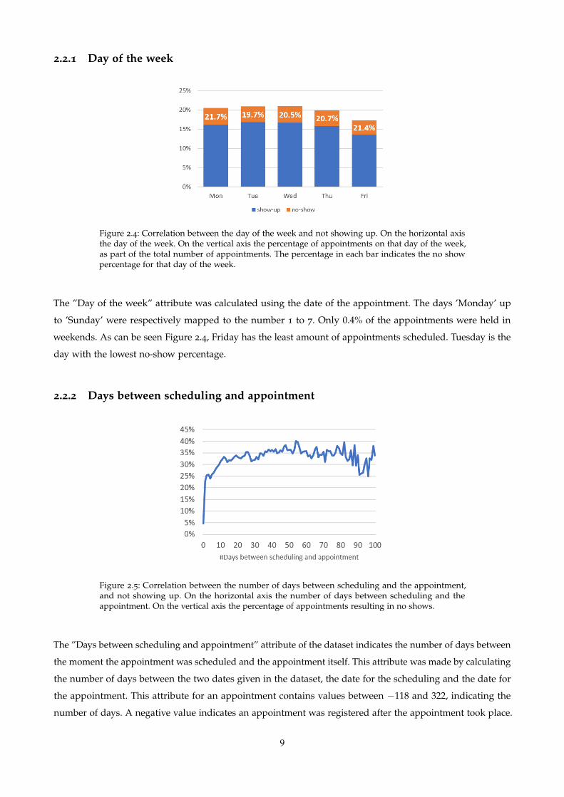
2.2.1 Day of the week

Figure 2.4: Correlation between the day of the week and not showing up. On the horizontal axisthe day of the week. On the vertical axis the percentage of appointments on that day of the week,as part of the total number of appointments. The percentage in each bar indicates the no showpercentage for that day of the week.

The ”Day of the week” attribute was calculated using the date of the appointment. The days ’Monday’ up

to ’Sunday’ were respectively mapped to the number 1 to 7. Only 0.4% of the appointments were held in

weekends. As can be seen Figure 2.4, Friday has the least amount of appointments scheduled. Tuesday is the

day with the lowest no-show percentage.

2.2.2 Days between scheduling and appointment

Figure 2.5: Correlation between the number of days between scheduling and the appointment,and not showing up. On the horizontal axis the number of days between scheduling and theappointment. On the vertical axis the percentage of appointments resulting in no shows.

The ”Days between scheduling and appointment” attribute of the dataset indicates the number of days between

the moment the appointment was scheduled and the appointment itself. This attribute was made by calculating

the number of days between the two dates given in the dataset, the date for the scheduling and the date for

the appointment. This attribute for an appointment contains values between −118 and 322, indicating the

number of days. A negative value indicates an appointment was registered after the appointment took place.

9

The average number of days between when the appointment was scheduled and when it was held for positive

values is 15. As can be seen in Figure 2.5, the appointments which have been scheduled less than 10 days prior

to the appointment have a relatively lower no-show percentage than appointments scheduled more than 10

days prior to the appointment.

2.2.3 Days since previous appointment

The ”Days since previous appointment” attribute of the dataset indicates the number of days since the previous

appointment of this patient. This attribute was made by calculating the number of days between the current

appointment and the most recent appointment of the patient. If no other appointment was found the number

of days was set to 0. This attribute for an appointment contains values between 0 and 688, indicating the

number of days. The average is 33.7 days.

2.2.4 Previous no shows

The ”Previous no shows” attribute of the dataset indicates the number of consecutive no-shows in a row a

patient has had in the past 3 months. This attribute was made by finding the maximum no shows in a row

prior to this appointment in the last 3 months. This attribute for an appointment contains values between 0

and 27, indicating the number of missed appointments. The average is 0.232.

2.2.5 Previous no shows percentage

The ”Previous no shows percentage” attribute of the dataset equals the previous no shows of a patient divided

by the total number of previous appointments. This attribute for an appointment contains values between 0

and 1. The average is 0.173.

2.2.6 Previous total appointments

The ”Previous total appointments” attribute of the dataset indicates the total number of appointments prior to

the current appointment. This attribute was made by iterating over the appointments of a patients and starting

with 0 adding +1 to each new appointment. This attribute for an appointment contains values between 0 and

396, indicating the total number appointments. The average is 10.4.

10

Chapter 3

Methods

3.1 Machine Learning algorithms

This section is an overview covering a number of machine learning algorithms used for classification purposes.

The following algorithms will be used on the dataset to test their capabilities on this type of data.

3.1.1 Logistic regression

Logistic regression is a machine learning algorithm used for predictions on target variables that are binary,

like the target of this research whether a patient will show up or not. Logistic regression is based on odds,

meaning that if p is the probability of a show-up, then 1− p is the probability of a no-show. The other variables

influence this probability in a non-linear way, other than in linear regression.

Logistic regression uses the principles of the logistic or Sigmoid function ( f (x) = 11+e−x ) to compute the effects

of variables on the target. Neural networks also use this function.

3.1.2 Decision tree

Predictive models based on decision trees make use of decision rules which are structured in a tree-like

model [9]. This means that, in order to get the prediction for a given sample, one follows the path specific for

that sample through the tree structure. For decision trees two components can make it more accurate in its

predictions: a deeper tree (more rules) or more complex decision rules.

Decision trees are built by repeatedly splitting the data until a final model is reached. To decide on what

the model should split next, or even if it should split at all, information gain in the form of the entropy is

computed.

11

Figure 3.1 shows an example of a decision tree. As can be seen, the leafs in a decision tree contain the predicted

values. Using this model, if you are female, the model predicts you will survive. These models can also be

used to predict the probability of (in this case) survival. For a female this is 0.73 or 73%, as can be seen in the

Figure 3.1.

Figure 3.1: Example of a decision tree. The leaves are the predicted classes, including theprobability and division. Source: upload.wikimedia.org/wikipedia/commons/f/f3/CART_tree_titanic_survivors.png

Advantages of decision trees include that they are easy to interpret and visualise and have low computing

cost. Disadvantages are that decision trees often overfit the data, making them bad at generalising and that

they can change completely with only small changes in the data.

3.1.3 Bagged decision tree

A bagged decision tree is actually a combination of multiple normal decision trees. The principle used to

combine these normal trees is called bootstrap aggregation. Results from all the trees used are then combined

to give one final prediction.

Bootstrap aggregating (Bagging) was created to improve the predictions made by machine learning algorithms.

It operates by running multiple instances of the chosen machine learning algorithm and combining their results.

For prediction of a numerical value it takes the average of the different instance outputs. For classification it

outputs the most common value [10].

In order to generate different outcomes from the different instances bootstrapping is used. Bootstrapping

is a collective name for methods computing random samples with the ability to replaces values in it. This

creates the possibility to have multiple copies of a value within each sample. Because it uses multiple similar,

but different copies it can help to prevent overfitting. The idea is that by combining different samples into

one outcome, a more stable and correct model can be created, although it can possibly also decrease the

performance of methods that are stable by itself.

12

3.1.4 Random forest

Random forests are very similar to bagged decision trees. The only difference is that random trees use an

adapted version of the decision tree, whereas bagged trees use the normal version. The difference is on the

splitting of (sub) branches. A normal decision tree would consider all the possible variables to split on, whereas

the random forest version only may choose from a random subset of these features [11]. For this reason

random forest has higher chances on getting more variation between it’s multiple trees.

3.1.5 Gaussian Naıve Bayes

The Gaussian Naıve Bayes algorithm uses a Naıve Bayes classifier, based on the assumption that all features

are independent of each other (naıve).

Bayes’ theorem

Bayes’ theorem can be used to calculate the probability that a situation occurs with relation to certain conditions

known in advance [12]. When classifying medical appointments, if no-show is related to a patients age, Bayes’

theorem could more accurately predict a no-show if the patient’s age is known.

The mathematical formula for Bayes’ theorem is: P(A|B) = P(B|A) ∗ P(A)/P(B) where P(A) and P(B) are

the probabilities for occurrence of respectively A or B independent of each other and P(A|B) and P(B|A) are

the probabilities of respectively A and B where the other one is true.

With the example in the medical appointment dataset the theorem would be as follows:

P(no-show|age) = P(age|no-show) ∗ P(no-show)/P(age)

Because Naıve Bayes takes the assumption that all variables are independent, it is relatively fast compared to

other techniques. On the other hand, this might make it less accurate since in a real-life dataset most variables

will be at least somewhat dependant on each other. Another disadvantage of Naıve Bayes is the fact that it

assumes a normal distribution for numerical values.

3.1.6 Neural networks

In essence a neural network is an algorithm which works similar to the human brain. It is constructed of

interlinked neurons. The connections between these neurons give the neural network its properties. Neural

networks appear in different forms and configurations, depending on the application. In this research a

feedforward neural network is used. This is the most standard neural network. This type of network has data

flowing in only one direction, meaning information only flows from input to output [12]. This type does not

contain any loops or cycles. As seen in Figure 3.2 all arrows point from input toward output.

13

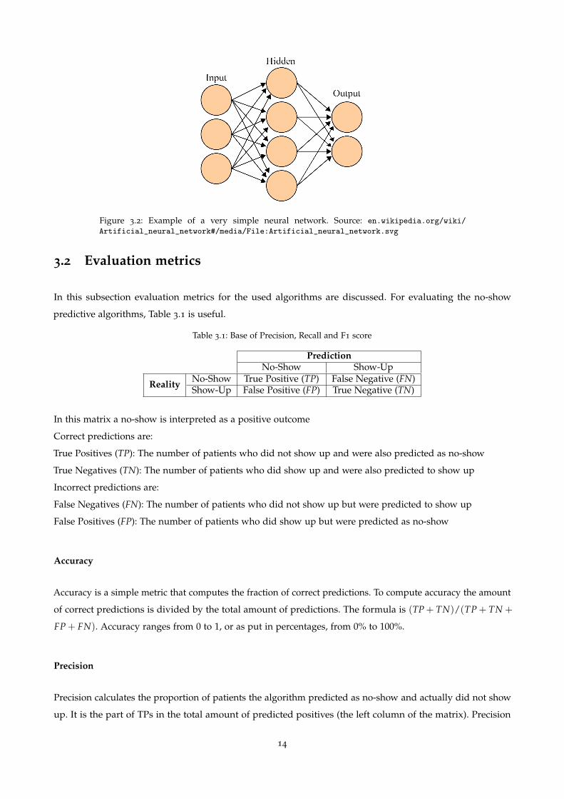
Figure 3.2: Example of a very simple neural network. Source: en.wikipedia.org/wiki/

Artificial_neural_network#/media/File:Artificial_neural_network.svg

3.2 Evaluation metrics

In this subsection evaluation metrics for the used algorithms are discussed. For evaluating the no-show

predictive algorithms, Table 3.1 is useful.

Table 3.1: Base of Precision, Recall and F1 score

PredictionNo-Show Show-Up

Reality No-Show True Positive (TP) False Negative (FN)Show-Up False Positive (FP) True Negative (TN)

In this matrix a no-show is interpreted as a positive outcome

Correct predictions are:

True Positives (TP): The number of patients who did not show up and were also predicted as no-show

True Negatives (TN): The number of patients who did show up and were also predicted to show up

Incorrect predictions are:

False Negatives (FN): The number of patients who did not show up but were predicted to show up

False Positives (FP): The number of patients who did show up but were predicted as no-show

Accuracy

Accuracy is a simple metric that computes the fraction of correct predictions. To compute accuracy the amount

of correct predictions is divided by the total amount of predictions. The formula is (TP + TN)/(TP + TN +

FP + FN). Accuracy ranges from 0 to 1, or as put in percentages, from 0% to 100%.

Precision

Precision calculates the proportion of patients the algorithm predicted as no-show and actually did not show

up. It is the part of TPs in the total amount of predicted positives (the left column of the matrix). Precision

14

indicates how often the algorithm incorrectly predicted a now-show. The formula is TP/(TP + FP). Precision

ranges from 0 to 1, or as put in percentages, from 0% to 100%.

Recall

Recall calculates the proportion of patients the algorithm predicted as no-show in the total amount of actual

no-shows (the top row of Table 3.1). Recall indicates how many no-shows the algorithm missed. The formula

is TP/(TP + FN). Recall ranges from 0 to 1, or as put in percentages, from 0% to 100%.

Basic performance indicators like accuracy are less useful when you work with skewed datasets (with a

no-show percentage of around 20 this medical appointment dataset is considered skewed). In the case of

skewed datasets accuracy is not a good representative of the actual performance. For example, for a dataset

with 100 positives and 9.900 negatives, an algorithm that always predicts negative will result in an accuracy of

99%, which is a bad indication. In these situations the F1 score is a better indicator.

F1 score

The F1 score is a weighted average of Precision and Recall and is calculated as their harmonic mean. The

formula is: 2 ∗ (Precision ∗Recall)/(Precision+ Recall). The F1 score ranges from 0 to 1, or as put in percentage,

from 0% to 100%.

For predictive algorithms additional metrics are relevant. Below Logarithmic Loss and the Brier score are

described.

Logarithmic Loss

Logarithmic Loss is, like a number of other loss functions, used for calculating the accuracy of classification

algorithms. It heavily penalises inaccurate predictions. In cases with two classes the formula to calculate

Logarithmic Loss (LL) is:

LL = − 1N ∑N

i=1[yi log pi + (1− yi) log(1− pi)]

Here N is the number of samples, yi the label of the sample (in our case 1 at a no-show) and pi is the estimated

probability of a no-show for sample: (1 ≤ i ≤ N). Logarithmic Loss ranges from 0 upwards, where 0 is the

best possible score.

Brier score

The Brier score is a straightforward mean squared difference function, where the difference is calculated

between the predicted outcome and the actual outcome for each item. In cases with two classes (0 and 1) the

formula to calculate the Brier score (BS) is:

15

BS = 1N ∑N

i=1(pi − ti)2

Here N is the number of samples, yi the label of the sample (in our case 1 at a no-show) and pi is the estimated

probability of a no-show for sample: (1 ≤ i ≤ N). The Brier score ranges from 0 to 1, where 0 is the best

possible score.

Receiver operating characteristic curve and Area under the curve

The Receiver operating characteristic (ROC) curve is created by plotting the True positive rate (recall) against

the False positive rate (FP/(FP + TN)), using multiple threshold settings. An imported metric derived from

this is the Area under the curve (AUC). The AUC ranges from 0 to 1, where 1 is the best possible score.

16

Chapter 4

Evaluation

This chapter deals with the way the experiments were conducted and discusses the results.

4.1 Splitting the data in a training- and testset

After trying multiple options for splitting the training and testset, the conclusion arose that the following split

was best suited for this type of problem. The testset is made up of all appointments in the last 3 months of the

dataset. This means that patients can occur in both the training- and testset. This decision was made on the

ground that, if this were used to make real predictions regarding no-shows, this data would also be available.

For a prediction about an appointment this week, all history previous to this week for the patient is available.

This means 21 months were left for the trainingset. The first 3 months of the trainingset were left out. These

appointments were used to start building up a patient history. The machine learning models were trained

with 18 of the total 24 months in the dataset.

4.2 Machine Learning algorithms configuration

Each algorithm has to be configured in some way. This section describes how the algorithms used in this

research were configured.

Logistic regression

The Logistic regression algorithm was configured to use the following cost function:

minw,c12 wTw + C ∑n

i=1 log(exp(−yi(XTi w + c)) + 1)

17

Decision tree

The Decision tree was configured to use ’information gain’ as the criterion on which splitting of branches is

based.The minimum of items on which the tree may split was set to 10, 000. Because the classes are imbalanced,

some balancing was conducted for use in the decision tree. This was done by inversely adding weight to the

classes.

Bagged decision tree

The Bagged decision tree was setup using 10 regular decision trees with the above mentioned parameters.

Random Forest

The Random Forest was setup using 10 regular decision trees with the above mentioned parameters.

Gaussian Naıve Bayes

The Gaussian Naıve Bayes algorithm does not have parameters to be configured.

Neural network

The neural network was configured as a feedforward network. The network was constructed to have 3 hidden

layers of 50 neurons each. It used the rectified linear unit function as activation function, defined as:

f (x) = max(0, x)

4.3 Metric results

After applying the algorithms to the dataset, using configurations mentioned above, the results in Table 4.1

are obtained. By looking at only the binary metrics, Accuracy and the F1 score, one can observe two distinct

categories. First, the tree-based algorithms, all of these have a fairly low accuracy and a reasonably high F1

score. Secondly, the rest with a high Accuracy and a low F1 score. Another notable observations is that all the

trees have nearly the same metric scores.

Looking at the probability metrics, Log Loss and AUC, one can see one highly notable thing. Based on the AUC

all algorithms based on trees and the neural network perform the same. This is confirmed by Figure 4.1, where

all the tree-based algorithms and the neural network follow the same curve. The neural network outperforms

the tree-based algorithms on the log loss. The logistic regression and Gaussian Naıve Bayes perfrom the worst

on predicting the probabilities.

18

Table 4.1: Metric results on the dataset

Algorithm Accuracy Precision Recall F1 Score Log Loss Brier Score AUC0 Logistic regression 0.79 0.46 0.05 0.08 0.48 0.15 0.70

1 Decision tree 0.61 0.33 0.82 0.47 0.59 0.21 0.76

2 Bagged decision tree 0.62 0.34 0.82 0.48 0.58 0.21 0.76

3 Random forest 0.60 0.33 0.85 0.47 0.59 0.21 0.76

4 Gaussian Naive Bayes 0.76 0.37 0.23 0.28 0.71 0.19 0.65

5 Neural network 0.79 0.60 0.07 0.13 0.44 0.14 0.76

Figure 4.1: The ROC curves resulting from the application of all algorithms to the dataset in asingle figure.

19

Chapter 5

Conclusions and Future Research

This chapter aims to answer the main question of this thesis using the subquestions, as well as pointing out

practical uses and future possibilities of this field of research.

At the start of this study, research questions were formed to which this research would be focused. These

questions were focused on the classification (binary) of no-shows. However during this research it was found

that predicting using the classification (binary) approach was not really feasible. The research questions will

still be answered, followed by extra information regarding the findings in predicting the probabilities of

no-shows.

5.1 Research questions

What is the best Machine learning approach for medical appointment no-show classification? In order to

answer the main question we distinguished two subquestions.

Which types of machine learning algorithms are applicable to this kind of classification problems?

While doing this research an extra criterion appeared for this type of data. The algorithms should also support

outputting probability predictions additional to binary predictions. For this reason a number of algorithms

were not taken into account. The algorithms used for this research are: Logistic regression; Decision tree;

Bagged decision tree; Random Forest; Gaussian Naıve Bayes; Neural network. All of these algorithms provide

a certain level of no-show prediction. However based on the F1 score and AUC, logistic regression does not

provide added value to solving the no-show problem.

20

Which type of machine learning algorithm performs the best on classifying medical appointment no-

shows?

In order to answer this question first binary classification was tested. The test results of algorithms used for

these binary predictions unfortunately proved binary classification to be quite hard. Because of this the switch

to predicting probabilities was made.

The test results of algorithms used for making probability predictions showed the tree-based algorithms and

the neural network outperformed the others, based on their AUC and log loss. With the neural network being

the best based on the log loss metric.

5.2 Probability predictions

The probability predictions seem to be of much more use as they better represent the data. They can easily be

aggregated to form a higher confidence interval over multiple appointments.

5.3 In practice

Probability predictions can be used in primary care to make predictions over multiple people. This can then

be used to perform overbooking and decrease the impact of no-show on the medical facilities. For these

predictions using the neural network will yield the highest results. However the decision tree is not far behind.

The decision tree has one major advantage as opposed to the neural network, the tree is visible whereas the

neural network is a black-box. This can be of high importance in companies.

5.4 Future work

Further research is required on the following parts within this subject:

Patterns in subsequent show / no-show behaviour.

It might be the case that people follow certain behaviour regarding their show / no-show ordering. For

instance it could be possible that a person (nearly) always shows up if his previous appointment resulted in a

no-show.

Application to real-world healthcare.

It should be further investigated how feasible using probability prediction is in a healthcare situation. How do

these prediction perform if compared to a fixed overbooking percentage.

21

The effect of the neighborhood on no-show behaviour.

One could assume that there are differences between certain neighborhoods regarding their no-show behaviour

on healthcare appointments.

22

Bibliography

[1] M. Smit, “No show, een onderzoek naar factoren die voorspellend zijn voor het niet verschijnen op de

eerste afspraak.,” 2007. Masters Thesis [In Dutch]. 1

[2] Merriam-Webster, “Definition of no-show.” https://www.merriam-webster.com/dictionary/no-show.

Accessed: 2018-06-15. 2

[3] Y. Huang and D. A. Hanauer, “Patient no-show predictive model development using multiple data

sources for an effective overbooking approach,” Applied clinical informatics, vol. 5, no. 03, pp. 836–860, 2014.

2

[4] B. P. Berg, M. Murr, D. Chermak, J. Woodall, M. Pignone, R. S. Sandler, and B. T. Denton, “Estimating

the cost of no-shows and evaluating the effects of mitigation strategies,” Medical Decision Making, vol. 33,

no. 8, pp. 976–985, 2013. 2

[5] J. Gier, “Missed appointments cost the u.s. healthcare system $150b each year,” Health Management

Technology, 2017. 2

[6] P. Kheirkhah, Q. Feng, L. M. Travis, S. Tavakoli-Tabasi, and A. Sharafkhaneh, “Prevalence, predictors and

economic consequences of no-shows,” BMC health services research, vol. 16, no. 1, p. 13, 2015. 2

[7] J. Hoppen, “Reducao de faltas em agendamentos medicos com inteligencia computacional caso de

vitoria-es.” https://aquare.la/pt/artigos/2017/01/30/reducao-de-faltas-em-agendamentos-medicos-com-

inteligencia-computacional-caso-de-vitoria-es/, 2017. [In Portuguese] Accessed: 2017-04-10. 4

[8] J. Hoppen, “No-show-issue-comma-300k.csv.” https://www.kaggle.com/joniarroba/noshowappointments,

2017. Accessed: 2017-04-10. 4

[9] J. R. Quinlan, “Induction of decision trees,” Machine Learning, vol. 1, pp. 81–106, 1986. 11

[10] L. Breiman, “Bagging predictors,” Machine Learning, vol. 24, no. 2, pp. 123–140, 1996. 12

[11] T. K. Ho, “Random decision forests,” in Proceedings of the Third International Conference on Document

Analysis and Recognition, vol. 1, pp. 278–282, IEEE, 1995. 13

[12] S. Russell and P. Norvig, Artificial Intelligence: A modern approach. third ed., 1995. 13

23

Appendices

24

Appendix A

Figure A.1: Correlation matrix between all valuesin the dataset and the extra added features. Valuesabsolute below 0.1 have been removed for clarity.

25