Ophthalmic Diagnostics Using Eye Tracking...
120
Degree project in Communication Systems Second level, 30.0 HEC Stockholm, Sweden RAFAEL ALDANA PULIDO Ophthalmic Diagnostics Using Eye Tracking Technology KTH Information and Communication Technology
Transcript of Ophthalmic Diagnostics Using Eye Tracking...

Degree project inCommunication Systems
Second level, 30.0 HECStockholm, Sweden
R A F A E L A L D A N A P U L I D O
Ophthalmic Diagnostics Using EyeTracking Technology
K T H I n f o r m a t i o n a n d
C o m m u n i c a t i o n T e c h n o l o g y

Ophthalmic Diagnostics UsingEye Tracking Technology
Master of Science Thesis
Rafael Aldana [email protected]
Supervisor: Gustaf Öqvist SeimyrExaminer: Prof. Gerald Q. Maguire Jr.
School of Information and Communication Technology (ICT)KTH Royal Institute of Technology
Stockholm, Sweden
February 15, 2012

i
Abstract
Human eyes directly reflect brain activity and cognition. The study of eyemovements and gaze patterns can therefore say a lot about the human brainand human behavior. Today eye tracking technology is being used to measureacuity of toddlers, to rehabilitate patients in intensive care, to detect if a personis lying or not, and to understand the cognitive level of a non-verbal person.
Current vision testing is mostly based on manual observation and subjectivemethods. With eye tracking technology eye movements can be tested inan automated way that increases reliability and reduces variability andsubjectivity.
Eye tracking technology allows for measuring eye movements and thereforequantitative comparisons of the progress in treatment can be made over thecourse of a patient’s therapy – enabling more effective therapy. This technologyalso enables standardized and automated processes that are more time- andcost-efficient. The most important advantages of this technology is that itis non-invasive and it is not necessary to stabilize the subject’s head duringtesting. These advantages greatly extend the set of subjects that can be studiedand reduce the cost and skills required for studying eye movements and gazepatterns.
This thesis has developed and evaluated a novel calibration procedure for aneye tracker. The development phase has included programming and integrationwith the existing application programming interfaces. The evaluation phaseincluded reliability and validity testing, as well as statistical analysis in termsof repeatability, objectivity, comprehension, relevance, and independence of theperformance of the Tobii T60/T120 Eye Tracker on healthy subjects.
The experimental results have shown that the prototype application givesthe expected benefits in a clinical setting. A conclusion of this thesis is thateye tracking technology could be an improvement over existing methods forscreening of eye alignment and diagnostics of ophthalmic disorders, such asstrabismus (crossed eyes) or amblyopia (lazy eye). However, applying thistechnology to clinical cases will require further development. This developmentis suggested as future work.


iii
Sammanfattning
En människas ögon speglar direkt hennes hjärnaktivitet och kognition. Attundersöka ögonens rörelsemönster kan därför säga mycket om den mänskligahjärnan och om mänskligt beteende. Idag används eye tracking-teknik för attmäta synskärpa hos småbarn, för att rehabilitera patienter i intensivvård, föratt upptäcka om en person talar sanning eller ej, och för att utvärdera denkognitiva nivån hos icke-verbala personer.
Nuvarande syntest bygger främst på manuella observationer och subjektivametoder. Med eye-tracking teknik kan ögonens rörelsemönster testas på ettautomatiserat sätt som ökar tillförlitligheten och minskar variabilitet ochsubjektivitet.
Eye tracking-tekniken tillåter kvantifiering av rörelsemönstrena och möjlig-gör jämförelser samt uppföljning av progression av behandlinger på etteffektivare sätt. Tekniken möjliggör även standardiserade och automatiseradeprocesser som är mer tids- och kostnadseffektiva. De mest intressantafördelarna med denna teknik är att den är icke-invasiv och att det inte ärnödvändigt att stabilisera subjektets huvud under testningen.
I denna tes har en ny metod för att kalibrera eye-tracking utrusning utveck-lats och utvärderats. Utvecklingsfasen bestod bland annat av programmeringsamt integration med befintliga API. I utvärderingsfasen ingick testning avreliabilitet och validitets samt statistisk analys för att undersöka repeterbarhet,objektivitet, förståelse, relevans och oberoende av Tobii T60/T120 Eye Trackerpå friska försökspersoner.
Resultat av experiment har visat att prototypen ger de förväntade förde-larna i en klinisk miljö. En slutsats av denna avhandling är att eye tracking-teknik kan förbättra befintliga metoder för screening av ögats anpassningoch för diagnostik av oftalmologiska sjukdomar, till exempel skelning elleramblyopi, om tekniken ytterligare utvecklas och förbättras.


v
Acknowledgements
I would like to sincerely thank my supervisors Jenny Grant, Peter Tiberg,and Gustaf Öqvist Seimyr. They introduced me to an interesting medicalapplication of software engineering and shared their good experience with me.We have had interesting discussions and they have provided feedback duringthe project, which I have enjoyed so much.
I would also like to thank my supervisor at KTH, Professor Gerald Q.Maguire Jr. I am glad he accepted to be my academic examiner since heconsidered this project very interesting. Gerald’s guidance has also beenessential in some steps of this thesis, such as the testing procedure of theprototype application and the analysis and presentation of results.
There are more people who also deserve great thanks. They are mycolleagues at Tobii Technology, all the involved people from KarolinskaInstitutet and S:t Eriks Ögonsjukhus, and all the test participants.
Finally I would like to thank my friends and my family, all of whom havebeen encouraging me during my stay in Stockholm.
Thank you all.


Contents
Contents vii
List of Acronyms and Abbreviations viii
List of Code Listings x
List of Figures xi
List of Tables xii
1 Introduction 11.1 The problem statement . . . . . . . . . . . . . . . . . . . . . . . . . 21.2 Goals . . . . . . . . . . . . . . . . . . . . . . . . . . . . . . . . . . . 21.3 Limitations . . . . . . . . . . . . . . . . . . . . . . . . . . . . . . . . 31.4 Audience . . . . . . . . . . . . . . . . . . . . . . . . . . . . . . . . . 41.5 Organization of the thesis . . . . . . . . . . . . . . . . . . . . . . . . 4
1.5.1 Research . . . . . . . . . . . . . . . . . . . . . . . . . . . . . . 51.5.2 Development and prototype building . . . . . . . . . . . . . . 51.5.3 Structure of this report . . . . . . . . . . . . . . . . . . . . . 6
2 Strabismus and amblyopia 92.1 Concomitant strabismus . . . . . . . . . . . . . . . . . . . . . . . . . 102.2 Incomitant strabismus . . . . . . . . . . . . . . . . . . . . . . . . . . 102.3 Amblyopia . . . . . . . . . . . . . . . . . . . . . . . . . . . . . . . . . 11
3 Previous work 133.1 Scleral search coil technique . . . . . . . . . . . . . . . . . . . . . . . 133.2 Image-processing techniques, video-oculography system . . . . . . . 143.3 Performance evaluations of remote and binocular 2D eye tracking
systems . . . . . . . . . . . . . . . . . . . . . . . . . . . . . . . . . . 153.4 Study of errors introduced by eye tracking systems . . . . . . . . . . 16
4 Hardware and experimental setup 174.1 The IEyetracker interface . . . . . . . . . . . . . . . . . . . . . . . . 19
vii

viii CONTENTS
4.2 Coordinate system . . . . . . . . . . . . . . . . . . . . . . . . . . . . 214.3 Available gaze data . . . . . . . . . . . . . . . . . . . . . . . . . . . . 224.4 Configuring the screen . . . . . . . . . . . . . . . . . . . . . . . . . . 264.5 Calibration . . . . . . . . . . . . . . . . . . . . . . . . . . . . . . . . 28
4.5.1 Calibration procedure . . . . . . . . . . . . . . . . . . . . . . 284.5.2 Calibration plot . . . . . . . . . . . . . . . . . . . . . . . . . 294.5.3 Calibration buffers . . . . . . . . . . . . . . . . . . . . . . . . 30
4.6 Tracking . . . . . . . . . . . . . . . . . . . . . . . . . . . . . . . . . . 324.7 Magnitudes and units . . . . . . . . . . . . . . . . . . . . . . . . . . 324.8 Test procedure . . . . . . . . . . . . . . . . . . . . . . . . . . . . . . 35
4.8.1 Environment . . . . . . . . . . . . . . . . . . . . . . . . . . . 354.8.2 Equipment . . . . . . . . . . . . . . . . . . . . . . . . . . . . 374.8.3 Workflow . . . . . . . . . . . . . . . . . . . . . . . . . . . . . 38
5 Description of the prototype application 415.1 Specification of the desired report . . . . . . . . . . . . . . . . . . . . 415.2 Workflow of Tobii Alignment . . . . . . . . . . . . . . . . . . . . . . 44
5.2.1 Calibration routines . . . . . . . . . . . . . . . . . . . . . . . 475.2.2 Tracking routine . . . . . . . . . . . . . . . . . . . . . . . . . 52
6 Evaluation 536.1 Study I – Measurement of 2D gaze points on the tracking area . . . 536.2 Study II – Measurement of angles of deviation between gaze and
target vectors . . . . . . . . . . . . . . . . . . . . . . . . . . . . . . . 566.3 Study III – Tobii Alignment validation against scleral search coil
technique . . . . . . . . . . . . . . . . . . . . . . . . . . . . . . . . . 666.3.1 Principles of operation of a scleral search coil . . . . . . . . . 666.3.2 Validation procedure . . . . . . . . . . . . . . . . . . . . . . . 696.3.3 Transformation from voltage to angle of deviation . . . . . . 706.3.4 Interpolation and decimation of a set of samples . . . . . . . 716.3.5 Correlation between the Tobii T120 Eye Tracker and SSC
performances . . . . . . . . . . . . . . . . . . . . . . . . . . . 746.3.6 Graphical comparison between the Tobii T120 Eye Tracker
and SSC performances . . . . . . . . . . . . . . . . . . . . . . 776.3.7 Influence of the changes in the pupil size . . . . . . . . . . . . 886.3.8 Discussion . . . . . . . . . . . . . . . . . . . . . . . . . . . . . 89
7 Conclusions and Future work 917.1 Discussion of the results . . . . . . . . . . . . . . . . . . . . . . . . . 917.2 Future work . . . . . . . . . . . . . . . . . . . . . . . . . . . . . . . . 92
Bibliography 95
A A diagram of the human eye 99

List of Acronyms and Abbreviations
API Application Programming InterfaceCALIB calibration data filecm centimeterCPU Central Processing UnitDHCP Dynamic Host Configuration ProtocolESO esotropiaETT Eye Tracking TechnologyEXE executable applicationEXO exotropiaFFT Fast Fourier TransformGB gigabyteGHz gigahertzHYPO hypotropiaHYPER hypertropiaHz hertzi.e. that isIP Internet ProtocolIR infraredkHz kilohertzLAN Local Area NetworkmA milliampereMbps megabit per secondms millisecondnm nanometerOD Oculus Dexter, right eyeORTHO orthotropiaOS Oculus Sinister, left eyePC Personal Computerrms Root Mean SquareSDK Software Development Kits secondSSC Scleral Search Coil
ix

x List of Acronyms and Abbreviations
TFT Thin-Film TransistorTRACK tracking data fileUCS User Coordinate SystemUSB Universal Serial BusVGA Video Graphics ArrayVOG video-oculography

List of Code Listings
4.1 The IEyetracker interface [36]. . . . . . . . . . . . . . . . . . . . . . 204.2 The Point2D class [36]. . . . . . . . . . . . . . . . . . . . . . . . . . 224.3 The Point3D class [36]. . . . . . . . . . . . . . . . . . . . . . . . . . 224.4 The GazeDataItem class [36]. . . . . . . . . . . . . . . . . . . . . . . 234.5 The XConfiguration class [36]. . . . . . . . . . . . . . . . . . . . . . . 274.6 The CalibrationPlotItem class [36]. . . . . . . . . . . . . . . . . . . . 314.7 The Calibration class [36]. . . . . . . . . . . . . . . . . . . . . . . . . 324.8 Precision of angular magnitude. . . . . . . . . . . . . . . . . . . . . . 345.1 The binocular calibration routine . . . . . . . . . . . . . . . . . . . . 485.2 The monocular calibration on the left eye routine . . . . . . . . . . . 495.3 The monocular calibration on the right eye routine . . . . . . . . . . 505.4 The Merge Calibratios routine . . . . . . . . . . . . . . . . . . . . . . 515.5 The Start Tracking routine . . . . . . . . . . . . . . . . . . . . . . . 526.1 Transformation from voltage to angle of deviation. . . . . . . . . . . 706.2 Linear interpolation. . . . . . . . . . . . . . . . . . . . . . . . . . . . 726.3 Sampling. . . . . . . . . . . . . . . . . . . . . . . . . . . . . . . . . . 736.4 Correlation in the changes in the signals. . . . . . . . . . . . . . . . . 756.5 Calculation of the correlation in the changes in two signals. . . . . . 766.6 Calculation of the average discarding not valid samples. . . . . . . . 76
xi

List of Figures
1.1 The planned development process. . . . . . . . . . . . . . . . . . . . . . 4
2.1 Graphical examples of concomitant strabismus. . . . . . . . . . . . . . . 10
3.1 The scleral search coil setting. Picture taken at Bernadottelaboratorietat S:t Eriks Ögonsjukhus during the Tobii Alignment validation againstSSC technique. . . . . . . . . . . . . . . . . . . . . . . . . . . . . . . . . 14
4.1 Pupil center corneal reflection. Adapted from [6]. . . . . . . . . . . . . . 184.2 A drawing of two subjects with bright and dark pupils each one. Adapted
from [6]. . . . . . . . . . . . . . . . . . . . . . . . . . . . . . . . . . . . . 184.3 Synchronization scenario. Adapted from [34, figure 12]. . . . . . . . . . 194.4 The User Coordinate System on a Tobii T60/T120 Eye Tracker. Adapted
from [34, figure 6]. . . . . . . . . . . . . . . . . . . . . . . . . . . . . . . 214.5 Schematic head movement box. Adapted from [34, figure 16]. . . . . . . 244.6 Gaze point and gaze vector. Adapted from [34, figure 7]. . . . . . . . . . 244.7 Screen configuration schematic. Adapted from [34, figure 17]. . . . . . . 264.8 A 9-point calibration plot example with data for the left eye. . . . . . . 304.9 A 9-point calibration plot example with data for the right eye. . . . . . 314.10 Angle of deviation decomposed into φ and θ. Adapted from [2, p. 6]. . . 334.11 The room used for the first two sets of tests. . . . . . . . . . . . . . . . 364.12 The location of the light sources. Adapted from [2, figure 22]. . . . . . . 374.13 A light meter is required in order to determine the illumination in the
test room. Adapted from [2, figure 22]. . . . . . . . . . . . . . . . . . . . 384.14 The Eyetrackers Found on the Network and the Eyetracker Status boxes. 40
5.1 The 9-point calibration pattern. The points are randomly shown one byone. . . . . . . . . . . . . . . . . . . . . . . . . . . . . . . . . . . . . . . 42
5.2 A graphical generalization of the Tobii Alignment report. . . . . . . . . 445.3 The basic screen layout of Tobii Alignment. . . . . . . . . . . . . . . . . 455.4 An example of the appearance of the Gaze Plotter. Note that boxes of
the same row have the same origin in the horizontal axis, whereas boxesof the same column have the same origin in the vertical axis. . . . . . . 47
xii

List of Figures xiii
6.1 Monocular calibration on subject #4 with 750 nm wavelength IRtransparent lens. . . . . . . . . . . . . . . . . . . . . . . . . . . . . . . . 54
6.2 Monocular calibration on subject #11 with 800 nm wavelength IRtransparent lens. . . . . . . . . . . . . . . . . . . . . . . . . . . . . . . . 54
6.3 Binocular calibration on subject #10. . . . . . . . . . . . . . . . . . . . 556.4 Average φL deviations for every subject, calibration, session, and test.
All measurements are expressed in degrees. Note that the plots ofbinocular calibration are scaled to a different range. . . . . . . . . . . . 57
6.5 Average θL deviations for every subject, calibration, session, and test. Allmeasurements are expressed in degrees. Note that the plots of binocularcalibration are scaled to a different range. . . . . . . . . . . . . . . . . . 58
6.6 Average φR deviations for every subject, calibration, session, and test.All measurements are expressed in degrees. Note that the plots ofbinocular calibration are scaled to a different range. . . . . . . . . . . . 59
6.7 Average θR deviations for every subject, calibration, session, and test.All measurements are expressed in degrees. Note that the plots ofbinocular calibration are scaled to a different range. . . . . . . . . . . . 60
6.8 Average vergence angle (φL −φR) for every subject, calibration, session,and test. All measurements are expressed in degrees. Note that the plotsof binocular calibration are scaled to a different range. . . . . . . . . . . 61
6.9 Linear regression for binocular calibration. All measurements areexpressed in degrees. . . . . . . . . . . . . . . . . . . . . . . . . . . . . . 63
6.10 Linear regression for MONO LR calibration. All measurements areexpressed in degrees. . . . . . . . . . . . . . . . . . . . . . . . . . . . . . 64
6.11 Linear regression for MONO RL calibration. All measurements areexpressed in degrees. . . . . . . . . . . . . . . . . . . . . . . . . . . . . . 65
6.12 Relationship between samples in a linear interpolator for L = 3. . . . . 726.13 Impulse response of a linear interpolator for L = 3. . . . . . . . . . . . . 736.14 Effect of a sampler for M = 8. . . . . . . . . . . . . . . . . . . . . . . . . 746.15 Correlation between both measurement techniques. . . . . . . . . . . . . 776.16 Binocular calibration and φ tracking on subject #1. . . . . . . . . . . . 786.17 Binocular calibration abd θ tracking on subject #1. . . . . . . . . . . . 796.18 Monocular calibration and φ tracking on subject #1. . . . . . . . . . . . 806.19 Monocular calibration abd θ tracking on subject #1. . . . . . . . . . . . 816.20 Vergence angle for subject #1. . . . . . . . . . . . . . . . . . . . . . . . 826.21 Binocular calibration and φ tracking on subject #2. . . . . . . . . . . . 836.22 Binocular calibration abd θ tracking on subject #2. . . . . . . . . . . . 846.23 Monocular calibration and φ tracking on subject #2. . . . . . . . . . . . 856.24 Monocular calibration abd θ tracking on subject #2. . . . . . . . . . . . 866.25 Vergence angle for subject #2. . . . . . . . . . . . . . . . . . . . . . . . 876.26 Comparison between the original and the modified T120 outputs. . . . . 88
A.1 A diagram of the human eye [14]. . . . . . . . . . . . . . . . . . . . . . . 99

List of Tables
4.1 Data validity codes. . . . . . . . . . . . . . . . . . . . . . . . . . . . . . 25
5.1 The location of the calibration points in 2D and 3D coordinates. . . . . 425.2 The location of the calibration points in 2D coordinates and degrees. . . 43
6.1 Mean and standard deviation values with respect to the correspondingtarget point for the nine cardinal positions and all the subjects. Valuesin red are out of the desired range (a deviation within the order ofmagnitude of a microsaccade may be ignored, and the implication of apositive vergence value is crossed fixation). . . . . . . . . . . . . . . . . 62
6.2 Binocular calibration procedure in a SSC setting. . . . . . . . . . . . . . 696.3 Monocular calibration procedure in a SSC setting. . . . . . . . . . . . . 696.4 Correlation between both measurement techniques. . . . . . . . . . . . . 776.5 Mean difference between both measurements expressed in degrees. . . . 89
xiv

Chapter 1
Introduction
Today eye tracking is a very innovative technology by which computers are ableto estimate with high accuracy where users are looking. Eye tracking technology(ETT) can be used in both analytical and interactive applications. Some of theseapplications are assessments, diagnostics, and rehabilitation within the field ofclinical ophthalmology.
An eye tracker estimates the point of gaze with high accuracy using imagesensor technology and mathematical algorithms that find the subject’s eyes. Inother words, the tracker works much like an ophthalmologist would if he/she face apatient and estimates where the subject is looking just by observing the subject’seyes.
For clinical use there is a range of eye movement data that contains valuablediagnostic information. This eye movement data can be objectively quantified andcompared to published data. Deviations that are related to a particular diagnosisor impairment(s) can be identified.
In the field of clinical ophthalmology applying ETT at specialist centers oroptometrists can provide a superior way of studying ocular motor behavior andvision deficiencies in comparison to current clinical techniques. The quantifiabledata could include:
• Saccadic performance, such as latency, overshoot, and undershoot.
• Fixation stability, such as drift.
• Smooth pursuit, such as asymmetries between eye movement and stimuli.
• Alignment, such as strabismus (uncontrolled inward or outward eye move-ment) or amblyopia (lazy eye) – further details are given in chapter 2.
• Nystagmus (rapid eye movements), such as the slope of the slow phase andamplitude of the fast phase – details of these phases can be found in [19, p.28].
1

2 CHAPTER 1. INTRODUCTION
1.1 The problem statementIn the field of ophthalmology, oculomotor behavior, cognitive visual function, andvision deficiencies have been studied from a qualitative eye-movement analysisapproach. In consequence, methodologies that rely on observation have been manualand variable, generally resulting in the identification of disease taking place at a latestage of disease progression.
As the dynamics of eye movement have been subjectively and qualitativelyanalyzed, it has been hard to compare such data to published data or deviationsrelated to a particular diagnosis. As a result, impairments can not be easilyidentified.
Eye movement studies in a subjective and manual way are variable andunreliable. Standardized but manual processes are not time- or cost-efficient. In thesame way, comparison, follow-up, and progression studies also need to be automatedso that they too can be more effective.
The method that has been categorized as the gold standard is the scleral searchcoil technique (SSC) [22, p. 137-145]. SSC provides an accurate, but expensive andinvasive method to study eye movements and eye movement deficits. Moreover, thesubject is required to place their chin on a chin rest in order to be stabilized duringtesting, what limits head movement. The result is a neither natural nor relaxedtest situation, this is especially importunate in research or diagnoses that involvechildren.
1.2 GoalsThis thesis was motivated by the following goals:
• Study of true eye movements
An eye tracker measures at high sampling rates compared to a microsaccade1
interval both the direction of gaze as well as the position of the eyes in spacewith high accuracy. This enables the calculation of head movements and, byextension, calculation of the true eye movements within the orbit of the eye.
• Quantification of eye movement data
ETT allow ophthalmologists to quantify the dynamics of eye movement data.This is useful when studying eye movement data as this data that containsvaluable diagnostic information. The possibility of objectively quantifyingsuch data facilitates comparison to published data and deviations related toa particular diagnosis or that identification of specific impairments.
1Microsaccades are small and involuntary eye movements that move the gaze back to the targetafter a drift. They can be as large as 1 degree and last for 0.3 seconds [18].

1.3. LIMITATIONS 3
• Reduction of variability and increased of efficiency
ETT enables eye movement studies in an objective and automated way thatincreases reliability and reduces variability. In vision research, as well asin clinical assessments of eye movements, automated processes could replacemanual observation. ETT can be used to implement standardized andautomated processes which are more time- and cost-efficient. The abilityto quantify eye movement data makes comparison, follow-up, and progressionstudies more effective.
• Provision of a non-invasive method with improved validity
ETT does not require placing any equipment on the subject’s head and allowsfor a great deal of free head movement. The result is a natural and relaxed testsituation, which is imperative in research or diagnoses that involve children.
In order to reach these goals, the following steps involved were undertaken inthis thesis:
• Investigation of the requirements for a clinical tool to test alignment with aneye tracker.
• Development of the required calibration procedure of an eye tracker and aprototype application, Tobii Alignment, programmed in C#. The applicationis self instructive and very simple to use in a clinical situation.
• Evaluation of the prototype in a clinical environment for a Tobii T60/T120Eye Tracker. This lead to a verification of the expected benefits.
1.3 LimitationsThis thesis excludes:
• Market research
However, the incidence of strabismus is 5-8% in the general population [10,p. 96] and amblyopia has been estimated to affect between 1% and 5% ofthe world population [3, p. 365–375], hence there should be a substantialpotential market in the area of clinical alignment testing methods.
• Cost analysis
The cost of a clinically suitable eye tracker has not been estimated. The costof the necessary development work (either in this thesis or for any furtherdevelopment) has not be estimated.

4 CHAPTER 1. INTRODUCTION
• A complete description of the ophthalmic disorders considered in this work
This thesis focuses on determining the new methods potential to address aspecification defined in conjunction with experts and clinicians in the areaat Karolinska Institutet. Although some information about these disordersis given in chapter 2 to facilitate the reader’s understanding of this thesis –details of the ophthalmic disorders are outside the scope of this work.
• Adjustments for different eye trackers
The application developed in this thesis works only with Tobii Technology’seye trackers. Technology provided access to their code and experts to enablethe development of this application.
• Evaluation of the prototype system in a clinical environment with patients
This thesis focuses on the development of a new method to provide repeatabil-ity, objectivity, comprehension, relevance, and independence. An evaluationwith patients was outside the scope of the project’s definition.
1.4 Audience
Vision researchers and software engineers interested in developing applications forETT hardware for clinical purposes could benefit from this thesis. This thesis mayalso be interesting for others who may wish to use ETT in their applications, suchas for games or assessing if the user is becoming tired.
1.5 Organization of the thesis
The overall development process for the prototype in this thesis is illustrated infigure 1.1.
Figure 1.1: The planned development process.
1.5. ORGANIZATION OF THE THESIS 5
1.5.1 Research
Some limited research in ophthalmology, vision test methods, and eye tracking hasbeen performed to gather background information about ophthalmology in general,vision evaluation tests, and gaze tracking. This has been done by reading relevantliterature, which is included in the bibliography, learning about the vision testprocedures at Berdanottelaboratoriet at S:t Eriks Ögonsjukhus, and asking questionsof the staff at Karolinska Institutet and Tobii Technology.
1.5.2 Development and prototype building
The prototype development process was divided into three major parts because ofthe vision test methodology: operant conditioning, testing, and showing results.
Requirement analysis – Specifying the report that the application must returnA few requirements were already defined by researchers at Karolinska Institutet
before this thesis project started had a clear vision of what they wanted from thenew vision test. This new test was supposed to produce at least the same resultsas the tests that are used today. Therefore, a small study of the methodologythat is currently being used was performed. The requirements were modified a bitduring the application development. The final requirement specification is given inchapter 5.
Design – Specifying what the parts will be and how they will fit togetherSome sketches and sequence diagrams were made before the start of the
development phase. The sequence diagrams were used to lay out the parts of thevision test and how they should be built. See section 5.2.
Implementation – Writing the codeThe prototype application has been developed in Microsoft Visual Studio 2010,
using C# .NET as the programming language. The Tobii Eye Tracker SoftwareDevelopment Kit (SDK) has been used to interface with the eye tracker during thetest. The prototype was tested and evaluated as it was being developed. Finally,the entire prototype was tested and evaluated against the gold standard method.See sections 3.1, 5.2, and 6.3.
Testing – Executing the application with test data for inputThe prototype was tested during development with three sets of tests. First,
tests were performed on sixteen adults to see if the tests would produce the sameresults when replicated. In this testing there was no calculation of angle of deviation,the results were simply the 2D gaze point sets as output by the SDK. Subsequently,tests were performed on twelve adults, most of whom had participated in theprevious test. This testing included calculation of angle of deviation. Finally,tests were performed on two adults in a SSC setting to see if there was correlationbetween the gaze data returned by both procedures. The first two sets of tests

6 CHAPTER 1. INTRODUCTION
were performed at Tobii Technology and the final set of tests were performed atBerdanottelaboratoriet at S:t Eriks Ögonsjukhus. The conditions of these tests areexplained in section 4.8.
Evaluation – Study of reliability and validity as well as statistical analysisThe results have been analyzed using MATLAB R2010b. All the gaze data were
analyzed to compute the mean and standard deviation values for each eye and thetarget point in every isolated test. The analysis shows that the tests produce thesame results when replicated on the same subject when considering both 2D gazepoints got from the SDK and angles of deviation obtained from computing gaze andtarget vectors. See chapter 6.
Maintenance – Repairing software defects and adding capabilitySoftware maintenance has been performed to a limited extent during the
development. Error testing of the different parts of the prototype has beenperformed in sufficiently for a complete prototype, but the complete user interfacehas not been tested. The development and testing of a more complete user interfacewill mostly occur after this thesis project, therefore further details of this userinterface are excluded from the thesis.
1.5.3 Structure of this report
Chapter 2 outlines the various types of strabismus and ocular motility disturbancesthat have been considered in this thesis. It contains basic information on each topic,but excludes in-depth discussion as this is beyond the scope of this work – for detailsthe reader is referred to [3, 4, 5, 7, 10, 15, 23, 27, 29, 41].
Chapter 3 reports on previous work which has been done in the area of alignmenttesting using ETT, including verification of system performance and methods fordata analysis. SSC, the method considered to be the gold standard, is presentedhere.
Chapter 4 introduces the Tobii T60/T120 Eye Tracker and its SDK. Thischapter includes a description of the magnitudes utilized and their units as wellas the input and output parameters.
Chapter 5 presents in detail the desired report that the software should output.This report’s contents were defined in the beginning of the thesis in conjunctionwith experts and clinicians in the area at Karolinska Institutet. The prototypesystem architecture designed and implemented during this thesis is explained inthis chapter.
Chapter 6 contains the evaluation performed for the system architecture andprototype presented in chapter 5. Three different sets of tests were made.

1.5. ORGANIZATION OF THE THESIS 7
Chapter 7 presents a discussion of the results presented in chapter 6 and drawssome conclusions. Finally, the excluded scope of this thesis is re-considered andpresented as suggestions for future work.


Chapter 2
Strabismus and amblyopia
This chapter outlines the various types of ophthalmic disorders that have beenconsidered in this thesis. In regard to figures in which both eyes appear, note thatthe eyes are placed as an ophthalmologist would observe when facing a patient.This is why the left eye is shown on the right and viceversa.
Strabismus is a condition in which one or more visual axis is not directed towardsthe fixation point [10, p. 96]. In fixing a distant point, the visual axes of both eyesnormally are aligned [33, p. 3]. This disorder may occur in one of two major forms:concomitant or incomitant.
In concomitant strabismus, the deviation is, within physiologic limits and for agiven fixation distance, the same in all directions of gaze. In this type of strabismus,all eye muscles function normally; there is simply an error in the position of the eyes.In incomitant strabismus, there is a paralysis of the nerve innervating extraocularmuscle. The deviation therefore varies in different directions of gaze, but is largerwhen the eyes are turned in the direction of action of the underacting or paralyticmuscle [7, 33].
In other words, we speak of concomitance when, in spite of the deviation, oneeye accompanies the other in all its excursions whereas incomitance implies thatthe angle of deviation changes with different positions of gaze.
Amblyopia signifies weak vision. At present, the word “amblyopia” is only rarelyused in connection with organically caused decreases in vision, such as tobacco-alcohol amblyopia or quinine amblyopia. Usually, amblyopia is considered to befunctional, meaning that it is reversible. However, there can also be a combinationof organic and functional causes as well and only when vision loss is reversible byexercises, is there proof of the functional nature of this amblyopia [33].
9

10 CHAPTER 2. STRABISMUS AND AMBLYOPIA
2.1 Concomitant strabismusThe following briefly explains the different types of concomitant strabismus thathave been considered in this thesis. Note that the absence of is technically referredto as orthotropia.
Esotropia is a condition in which one or other eye deviates nasally [10].
Exotropia is a condition in which one or other eye deviates outwards [10].
Hypertropia is a disorder in which one or other eye is rotated upwards [10].
Hypotropia is a disorder in which one or other eye is rotated downwards [10].
(a) Esotropia. (b) Exotropia.
(c) Hypertropia. (d) Hypotropia.
Figure 2.1: Graphical examples of concomitant strabismus.
2.2 Incomitant strabismusIncomitant strabismus is associated with defective movement of the eye or withasymmetrical accommodative1 effort [10]. This condition may be found inassociation with many disorders. It can be congenital or acquired.
Congenital incomitance can be caused by abnormal innervation, trauma eitherduring gestation or delivery, inflammation either neonatal or antenatal, developmen-tal abnormality, muscle insertions to the eyeball or to the orbital contents, fibrosis,adhesions either intermuscular or muscle to orbit, etc.[10]
Acquired incomitance can be caused by trauma, multiple sclerosis, hypertension,space-occupying lesions, diabetes, fractures, n euromuscular junction, muscle fibremembrane, muscle fibre contents, etc.[10]
1Accommodation is the process by which the refractive power of the eyes is altered to ensure aclear retinal image [7].

2.3. AMBLYOPIA 11
2.3 AmblyopiaAmblyopia is a condition of diminished visual form sense which is not a result of anyclinically demonstrable anomaly of the visual pathway and which is not relieved bythe elimination of any defect that constitutes a dioptric obstacle to the formationof the foveal2 image [10].
Amblyopia is caused by inadequate stimulation of the visual system during thecritical period of visual development in early childhood, less than eight years. Thisis most marked under the age of two years [31]. Amblyopia may be unilateral orbilateral and the cause may be anyone or a combination of the following factors:
Light deprivation. There is no stimulus to the retina3. This is uncommon as itis likely that some light enters the eye even in dense cataract4.
Form deprivation. The retina receives a defocused image as with refractiveerrors.
Abnormal binocular interaction. Non-fusible images fall on each fovea as withstrabismus.
The prognosis for achieving good visual acuity decreases when more than oneof these factors are present together [10].
2The fovea is a part of the eye, located in the center of the macula region of the retina [26, p.1698–1705][30]. The fovea is responsible for sharp central vision, which is necessary in humans forfixating when visual detail is of primary importance.
3The retina is a light-sensitive tissue lining the inner surface of the eye [29].4A cataract is a clouding that develops in the crystalline lens of the eye or in its envelope,
varying in degree from slight to complete opacity and obstructing the passage of light [11].


Chapter 3
Previous work
A lot of work has been carried out in the area of ETT solutions for assessment anddiagnosis within ophthalmology. This chapter presents a small sample of this workto provide content for the work done in this thesis project.
3.1 Scleral search coil techniqueThe method that until today has been categorized as the gold standard is the scleralsearch coil technique (SSC) [22, p. 137-145]. It provides an accurate, but expensiveand invasive method to study eye movements and eye movement deficits. It doesthis by recording horizontal, vertical, and torsional eye movements binocularly. Itrequires applying a coil attached to a silicon contact lens to the subject’s sclera(white part of the eye) that picks up an induced voltage according to its positionin a magnetic field. The SSC apparatus is shown in figure 3.1.
Because the coil is attached to a lens attached to the subject’s sclera, the subjectneeds to be administered a local anesthesia and is required to place their chin on achin rest or use a bite bar in order to stabilize his/her head during testing. Moreover,SSC causes effects such as ocular discomfort, hyperaemia1 of the bulbar conjunctiva(a clear mucous membrane that covers the sclera and lines the inside of the eyelids),and reduction in visual acuity, among other effects. The result is a neither naturalnor relaxed test situation, this is especially importunate in research or tests thatinvolve children or test that require a long time to perform.
As the SSC is invasive and complex to setup, this method has been limitedexclusively to a strict research settings. In contrast, using ETT in a more clinicalenvironment the requirements of the procedure are different, i.e., the quantity ofpatients increases – hence the time for setup, calibration, and tracking proceduresdiminishes.
1Hyperaemia or hyperemia is an increase of blood flow. It is a regulatory response, allowingchanges in blood supply through vasodilation. It manifests as redness of the eye, because of theengorgement of vessels with oxygenated blood [27].
13

14 CHAPTER 3. PREVIOUS WORK
This thesis compares the scleral search coil and the Tobii T120 Eye Trackerusing tests on two volunteers aged 26 and 36 years old to analyze its performance interms of linearity, accuracy, and testing with both monocular and binocular tests.
Figure 3.1: The scleral search coil setting. Picture taken at Bernadottelaboratorietat S:t Eriks Ögonsjukhus during the Tobii Alignment validation against SSCtechnique.
3.2 Image-processing techniques, video-oculographysystem
Another system for measuring eye movements in three dimensions is the video-oculography system (VOG). This technique stems from photographic and cinemato-graphic recordings of the eye for measuring pupil size some decades ago. In thelate 1950s this method was refined and also used for measuring eye movements, inaddition to be a pupillometer [4, p. 47–48]. The sampling frequency was limited to25 Hz, which made it difficult to measure saccades [18]. VOG operates by trackingthe pupil center as an indicator of eye position.

3.3. PERFORMANCE EVALUATIONS OF REMOTE AND BINOCULAR 2D EYETRACKING SYSTEMS 15
The term VOG has been used for the image-processing techniques that alsomeasure torsional eye movements2. Today VOG systems work with small videocameras mounted in a mask that also includes some IR-emitting diodes to providethe necessary lighting. Analysis of the data from these cameras utilizes one of twodifferent principles: a two-dimensional correlation technique requiring the selectionof at least two landmarks on the surface of the iris or a polar correlation techniquewhich measures (and saves) a natural luminance profile from a sector of the iris.This saved luminance profile is then compared with the images frame-by-frame andthe degree of torsion is measured [4, p. 47–48].
To performance of the VOG system is about 0.02o, 0.01o, and 0.025o for thevertical, horizontal, and torsional components respectively. The system behavesrobustly within an angular range of ±25o for horizontal and vertical movements.The system’s biggest disadvantage is its low sampling frequency. Unfortunately, thissampling frequency is too low to properly study rapid movements like nystagmus3and saccades [4, p. 47–48]. This disadvantage is overcome by using systems withhigh speed cameras, specifically the Tobii T60/T120 Eye Tracker.
3.3 Performance evaluations of remote and binocular 2Deye tracking systems
Multiple studies have been performed to analyze the performance of eye trackerson healthy subjects in terms of linearity, accuracy, and testing with monocular andbinocular setups. The purpose was to understand the potential use of ETT indifferent clinical applications.
A performance evaluation of a remote and binocular 2D eye tracking system,including a linearity testing, optical filter testing, and a comparison between theSSC and the eye tracker on many test subjects between 16-30 years old with novision disabilities has been carried out by Alexander Hultman in [24]. In all teststhe stimuli were presented in 48 areas using a 17-inch TFT monitor. Each stimuluswas presented with a duration of less than 3 seconds. Two methods were used todescribe linearity. One method described linearity as a line of regression plus theR2-value. For each area the mean, of approximately 120 recorded samples, describedthe accuracy of the eye tracker. The second method described linearity as the errorof linearity as a percentage.
The correlation between the amplitude of each stimulus and the measured eyemovement was determined to be linear, which is close to the theoretically optimalcurve in both the horizontal and verticual plane. Even though the SSC has asignificantly lower standard deviation, the true line of sight could not be accessed
2The prototype application implemented in this thesis only reports horizontal and verticaldeviations.
3Nystagmus is a condition in which the eyes cannot be held still but have a constant tremulousmovement [33, p. 128].

16 CHAPTER 3. PREVIOUS WORK
more accurately, due to the uncertainty of fixation stability, as determined with theSSC rather than the eye tracker. As a conclusion was, ETT can be used for accuratetracking of 2D eye movements. This presupposed an acceptable calibration of eachtest subject the method could be configured with different stimulus configurationsthat could be used in medical experiments, such as visual acuity tests.
The thesis presented in this document also performed linearity testing andoptical filter testing. Performances of optical transparent lenses of 750 and 800 nmwavelength were compared with each other for a monocular setup. However, thestimuli were presented only in 9 areas with a duration of 2.2 seconds each, as asspecified by researchers at Bernadottelaboratoriet at S:t Eriks Ögonsjukhus. Gazedata were sampled only during one second in the middle of such interval. For eacharea the mean and the standard deviation of approximately 60 or 120 recordedsamples, depending on whether the eye tracker used was a Tobii T60 or T120,described their accuracy.
3.4 Study of errors introduced by eye tracking systemsMeasuring of eye movements regarding which types of errors different eye trackingsystems introduce was done by Magnus Olsson [13]. He showed how one can usecurve fitting to get a general idea of how the data has been altered by the eyetracking system and also how one can correct it afterwards.
The result was a program called LINEA that has been developed together withresearchers at Bernadottelaboratoriet at S:t Eriks Ögonsjukhus. The goal was tocorrect the errors introduced by various eye tracking systems in a general way.As such this software managed to correct errors independent of which system wasthe cause or the magnitude and type of the error. Many attempts were made tosolve the problem. One of them was to describe the non linearity using a surfacez = f(x, y). This was presented as the optimal solution, but it failed in one majorway – as the author was not able to fit a surfaze z to a set of arbitrary fixationpoints. Another attempt was to skip pseudo axes completely and only use the baseaxes as references, but this resulted lower accuracy since the skewness was also lessaccurately described.
In the thesis presented in this document the angles of deviation and vergence4
were calculated disregarding the possible errors the eye tracker could introduce.This work sought to describe linearity and accuracy by looking at the mean andstandard deviation values of all gaze point sets, assuming an accuracy and a driftof 0.5 and 0.1 degrees respectively – as specified by the vendor [37].
4The vergence angle is defined as the difference between the rotation about the vertical axisof the left and the right eye. Using the magnitudes described in section 4.7, the vergence angle isdefined as v = φL − φR.
Chapter 4
Hardware and experimental setup
This chapter explains the knowledge needed to develop the prototype using theTobii T60/T120 Eye Tracker. There is also a description of the input and outputparameters, as well as the magnitudes utilized and their units.
Figure 4.1 illustrates how an eye tracker works. The Tobii T60/T120 EyeTracker is based on the principle of corneal-reflection tracking1 [6]. This processinvolves the following steps:
• One or several near-infrared illuminators, invisible to the human eye, createreflection patterns on the cornea of the eyes.
• At high sampling rates, one or more image sensors record an image of thesubject’s eyes.
• Image processing is used to find the eyes, detect the exact position of thepupil and/or iris, and identify the correct reflections from knowledge of theilluminators and their exact positions.
• A mathematical model of the eye is used to calculate the eyes’ position inspace and the point of gaze.
In this thesis project, infrared (IR) light transparent lenses were used to conductmonocular calibration in such a way the subject cannot fixate with the occluded eyewhereas the eye tracker’s sensors can still find that eye. Two IR transparent lenseswith different wavelength (750 nm and 800 nm respectively) provided by productionstaff working at Tobii Technology, who recommended these wavelength values, wereused to occlude the subject’s corresponding eye.
1The cornea is the transparent front part of the eye that covers the iris, pupil, and anteriorchamber. Together with the lens, the cornea refracts light, with the cornea accounting forapproximately two-thirds of the eye’s total optical power [15].
17

18 CHAPTER 4. HARDWARE AND EXPERIMENTAL SETUP
Figure 4.1: Pupil center corneal reflection. Adapted from [6].
Figure 4.2 shows two cases of different pupil color intensity. The Tobii T60/T120Eye Tracker uses two different illumination setups with pupil corneal reflection eyetracking to calculate the gaze position. It can accommodate larger variations inexperimental conditions and ethnicity than an eye tracker that uses only one of thetechniques described below[6]:
• Bright pupil eye tracking. Illuminators are placed close to the optical axis ofthe imaging sensor, which causes the pupil to appear lit up (this is the samephenomenon that causes red eyes in photos).
• Dark pupil eye tracking. Illuminators are placed away from the optical axiscausing the pupil to appear darker than the iris.
Figure 4.2: A drawing of two subjects with bright and dark pupils each one. Adaptedfrom [6].

4.1. THE IEYETRACKER INTERFACE 19
Figure 4.3 illustrates the scenario where the prototype application and the eyetracker are linked each other. Note that the application controls the display, whilethe ETT computes the subject’s gaze.
�������������
���������
��� � ���
Figure 4.3: Synchronization scenario. Adapted from [34, figure 12].
4.1 The IEyetracker interface
The Tobii SDK consists of a core library with a C-style interface. On top of thiscore library they have created language specific bindings that make it possible toaccess the eye tracker functionality from multiple languages [34, p. 10]. They haveimplemented many interfaces, but the most important interface to this project isthe IEyetracker interface. Listing 4.1 shows this interface.

20 CHAPTER 4. HARDWARE AND EXPERIMENTAL SETUP
Listing 4.1: The IEyetracker interface [36].#region Assembly Tobii . Eyetracking . Sdk . dll , v2 . 0 . 5 0 7 2 7#endregion
us ing System ;us ing System . Collections . Generic ;
namespace Tobii . Eyetracking . Sdk{
p u b l i c i n t e r f a c e IEyet racker : I D i s p o s a b l e{
bool RealTimeGazeData { get ; s e t ; }
event EventHandler<Cal ibrat ionStartedEventArgs > CalibrationStarted ;event EventHandler<Calibrat ionStoppedEventArgs> CalibrationStopped ;event EventHandler<ConnectionErrorEventArgs> ConnectionError ;event EventHandler<FramerateChangedEventArgs> FramerateChanged ;event EventHandler<GazeDataEventArgs> GazeDataReceived ;event EventHandler<HeadMovementBoxChangedEventArgs> ←↩
HeadMovementBoxChanged ;event EventHandler<XConfigurationChangedEventArgs> ←↩
XConfigurationChanged ;
void AddCalibrationPoint ( Point2D pt ) ;void AddCalibrationPointAsync ( Point2D pt , EventHandler<←↩
AsyncCompletedEventArgs<Empty>> responseHandler ) ;void ClearCalibration ( ) ;void ComputeCalibration ( ) ;void ComputeCalibrationAsync ( EventHandler<AsyncCompletedEventArgs<←↩
Empty>> responseHandler ) ;void DumpImages ( i n t count , i n t frequency ) ;void EnableExtension ( i n t extensionId ) ;I L i s t <f l o a t > EnumerateFramerates ( ) ;Author izeChal lenge GetAuthorizeChallenge ( i n t realmId , I L i s t <int > ←↩
algorithms ) ;I L i s t <Extension> GetAvailableExtensions ( ) ;C a l i b r a t i o n GetCalibration ( ) ;byte [ ] GetDiagnosticReport ( i n t includeImages ) ;I L i s t <Extension> GetEnabledExtensions ( ) ;f l o a t GetFramerate ( ) ;HeadMovementBox GetHeadMovementBox ( ) ;bool GetLowblinkMode ( ) ;PayPerUseInfo GetPayperuseInfo ( ) ;Uni t In fo GetUnitInfo ( ) ;s t r i n g GetUnitName ( ) ;XConf igurat ion GetXConfiguration ( ) ;void RemoveCalibrationPoint ( Point2D pt ) ;void SetCalibration ( C a l i b r a t i o n calibration ) ;void SetFramerate ( f l o a t framerate ) ;void SetLowblinkMode ( bool enabled ) ;void SetUnitName ( s t r i n g name ) ;void SetXConfiguration ( XConf igurat ion configuration ) ;void StartCalibration ( ) ;void StartTracking ( ) ;void StopCalibration ( ) ;void StopTracking ( ) ;void ValidateChallengeResponse ( i n t realmId , i n t algorithm , byte [ ] ←↩
responseData ) ;}
}

4.2. COORDINATE SYSTEM 21
4.2 Coordinate system
All of the data available from Tobii Eye Trackers that describe spatial coordinatesare given in the User Coordinate System (UCS). This coordinate system uses unitsof millimeters from an origin at the center of the frontal surface of the eye tracker.
The coordinate axes are oriented as shown in figure 4.4: the x-axis pointshorizontally towards the user’s right (green axis), the y-axis points verticallytowards the user’s up (red axis), and the z-axis points towards the user (blue axis),perpendicular to the filter surface [34, p. 22–23]. Note that the eye tracker itself islocated in the monitor’s bezel below the middle of the display’s screen.
Figure 4.4: The User Coordinate System on a Tobii T60/T120 Eye Tracker.Adapted from [34, figure 6].

22 CHAPTER 4. HARDWARE AND EXPERIMENTAL SETUP
4.3 Available gaze data
The possibility to collect gaze data is probably the most interesting functionalityprovided by the SDK. The SDK’s API makes it possible to subscribe to a streamof data that will arrive at the eye tracker’s sampling frequency, which can be set toeither 60 or 120 Hz.
This data will be used as input parameters when calculating angles of deviation.Some of these data are 2D and 3D point objects represented by two or three doublevalues respectively. They are implemented as using the Point2D and Point3Dclasses (see listing 4.2 and listing 4.3 respectively).
Listing 4.2: The Point2D class [36].#region Assembly Tobii . Eyetracking . Sdk . dll , v2 . 0 . 5 0 7 2 7#endregion
us ing System ;
namespace Tobii . Eyetracking . Sdk{
p u b l i c s t r u c t Point2D{
p u b l i c Point2D ( double x , double y ) ;
p u b l i c double X { get ; s e t ; }p u b l i c double Y { get ; s e t ; }
p u b l i c o v e r r i d e s t r i n g ToString ( ) ;}
}
Listing 4.3: The Point3D class [36].#region Assembly Tobii . Eyetracking . Sdk . dll , v2 . 0 . 5 0 7 2 7#endregion
us ing System ;
namespace Tobii . Eyetracking . Sdk{
p u b l i c s t r u c t Point3D{
p u b l i c Point3D ( double x , double y , double z ) ;
p u b l i c double X { get ; s e t ; }p u b l i c double Y { get ; s e t ; }p u b l i c double Z { get ; s e t ; }
p u b l i c o v e r r i d e s t r i n g ToString ( ) ;}
}

4.3. AVAILABLE GAZE DATA 23
Each sample consists of a GazeDataItem class object [34, p. 32–34]. TheGazeDataItem class is shown in listing 4.4. The elements of such an object aredescribed below.
Listing 4.4: The GazeDataItem class [36].#region Assembly Tobii . Eyetracking . Sdk . dll , v2 . 0 . 5 0 7 2 7#endregion
us ing System ;
namespace Tobii . Eyetracking . Sdk{
p u b l i c c l a s s GazeDataItem : IGazeDataItem{
p u b l i c GazeDataItem ( DataTree xdsGazeData ) ;
p u b l i c Point3D LeftEyePosition3D { get ; }p u b l i c Point3D LeftEyePosition3DRelative { get ; }p u b l i c Point2D LeftGazePoint2D { get ; }p u b l i c Point3D LeftGazePoint3D { get ; }p u b l i c f l o a t LeftPupilDiameter { get ; }p u b l i c i n t LeftValidity { get ; }p u b l i c Point3D RightEyePosition3D { get ; }p u b l i c Point3D RightEyePosition3DRelative { get ; }p u b l i c Point2D RightGazePoint2D { get ; }p u b l i c Point3D RightGazePoint3D { get ; }p u b l i c f l o a t RightPupilDiameter { get ; }p u b l i c i n t RightValidity { get ; }p u b l i c long TimeStamp { get ; }
}}
• The Time Stamp is a value that indicates the time when a specific gaze datasample was obtained by the eye tracker. This value should be interpreted asa 64 bit unsigned microsecond timer starting from some unknown point intime. The source of this time stamp is the internal clock in the eye trackerhardware. In a typical use case, such as the one implemented in this prototypeapplication, this time stamp is used to synchronize the gaze data stream whenthe first stimuli was presented on the computer screen. How this is done isdescribed in chapter 5.
• The Eye Position is provided for the left and right eye individually anddescribes the position of each eyeball in 3D space. Three floating point valuesare used to describe the x, y, and z coordinate respectively. The position isspecified in the UCS coordinate system. If a subject wearing glasses and hasa cornea that diverts by a few percent this will highly affect the accuracy –by up to 17% [37].

24 CHAPTER 4. HARDWARE AND EXPERIMENTAL SETUP
• The Relative Eye Position is provided for the left and right eye individuallyand gives the relative position of the eyeball in the head movement box volumeas three normalized coordinates (see figure 4.5). The head movement boxis an imaginary box in which a user can move his/her head and still betracked by the device. This information can be used to help the user positionhimself/herself in front of the tracker.
�
�
�
�
��
�
�� ������
Figure 4.5: Schematic head movement box. Adapted from [34, figure 16].
• The Gaze Point is provided for the left and right eye individually and describesthe position of the intersection between a line originating from the eye’sposition in the same direction as the gaze vector and the tracking plane. Thisis illustrated in figure 4.6. The gaze vector is not explicitly provided in thegaze data stream, but can easily be computed by substracting the 3D gazepoint and the 3D eye position and normalizing the resulting vector.
�����������
����������
���������� �
������ ����� �
Figure 4.6: Gaze point and gaze vector. Adapted from [34, figure 7].

4.3. AVAILABLE GAZE DATA 25
• The Relative Gaze Point is provided for the left and right eye individuallyand corresponds to the two dimensional position of the gaze point within thetracking plane. The coordinates are normalized to [0,1] with the point (0,0) inthe upper left corner from the user’s point of view. The x-coordinate increasesto the right and the y-coordinate increases towards the bottom of the screen.
• The Validity Code is an estimate of how certain the eye tracker is that thedata given for an eye really originates from that eye. When the tracker findstwo eyes in the camera image, identifying which one is the left and which oneis the right eye is very straightforward. Similarly the case when no eyes arefound at all is really simple. The most challenging case is when the trackeronly finds one eye in the camera’s image. When that happens, the imageprocessing algorithms tries to deduce if the eye in question is the left or theright one. This is done by referring to previous eye positions, the positionin the camera sensor and certain image features. The validity codes describethe outcome of this deduction. The validity codes can only appear in certaincombinations. These combinations and their interpretations are summarizedin table 4.1. The validity codes can be used to filter out data that is mostlikely incorrect. Normally it is recommended that all samples with validitycode 2 or higher are removed or ignored, but only samples with validity code0 are considered in the prototype application implemented.
Table 4.1: Data validity codes.
��������LeftRight 0 1 2 3 4
0 Found twoeyes.
Found mostprobable theleft eye only.
1Found
probably theleft eye only.
2Found oneeye withoutany certainty.
3
Foundprobably theright eyeonly.
4
Found mostprobably theright eyeonly.
No eyesfound.

26 CHAPTER 4. HARDWARE AND EXPERIMENTAL SETUP
• The Pupil Diameter data is provided for the left and the right eye individuallyand is an estimate of the pupil size in millimeters. The Tobii Eye Trackerstry to measure the true pupil size, i.e., the algorithms take into account themagnification effect given by the spherical cornea as well as the distance tothe eye.
4.4 Configuring the screenTo compute angles between vectors described by the corresponding eye positionand any point on the eye tracker screen, it is necessary to configure the eye trackingarea geometry. The SDK contains functions to learn the so called x-configurationparameters. Before starting to calculate such angles, it is necessary to know therelative position of the tracking area in relation to the eye tracker screen. Thetracking plane is described by three points in space, the upper left, upper rightand lower left corner points of the eye tracker screen. These three points mustbe described in the UCS coordinate system as illustrated by the red vectors infigure 4.7.
���������
�������
�������� �
��
�
�����������������
Figure 4.7: Screen configuration schematic. Adapted from [34, figure 17].
As the Tobii T60/T120 Eye Tracker includes a 17-inch TFT monitor, thesethree points are mechanically fixed and there positions already measured, thus thecoordinates of these three points can be returned by the SDK. They will be usedas input parameters in conjunction with the gaze data when calculating angles ofdeviation. The XConfiguration class is shown in listing 4.5.

4.4. CONFIGURING THE SCREEN 27
Listing 4.5: The XConfiguration class [36].#region Assembly Tobii . Eyetracking . Sdk . dll , v2 . 0 . 5 0 7 2 7#endregion
us ing System ;
namespace Tobii . Eyetracking . Sdk{
p u b l i c c l a s s XConf igurat ion{
p u b l i c XConf igurat ion ( ) ;
p u b l i c Point3D LowerLeft { get ; s e t ; }p u b l i c Point3D UpperLeft { get ; s e t ; }p u b l i c Point3D UpperRight { get ; s e t ; }
}}
The GetXConfiguration() method of the IEyetracker interface returns thex-configuration parameters. Let P , Q, and R be the upper left, upper right, andlower left corner 3D points of the eye tracker’s screen respectively. After calling thismethod on the Tobii T60/T120 Eye Tracker, the following 3D points are returned:
P (x, y, z) = (−169, 287.6, 93.78)
Q(x, y, z) = (169, 287.6, 93.78)
R(x, y, z) = (−169, 31.8, −4.41)
Let O be the origin in the UCS. Let �H and �V be the horizontal and verticaldirections on the eye tracker screen respectively. �H and �V are calculated as follows:
�H(x, y, z) = �PQ = �OQ − �OP = (Qx − Px, Qy − Py, Qz − Pz) (4.1)
�V (x, y, z) = �PR = �OR − �OP = (Rx − Px, Ry − Py, Rz − Pz) (4.2)
Looking at the values of P , Q and R for the Tobii T60/T120 Eye Tracker wecan see that:
Px = −Qx = Rx (4.3)
Py = Qy (4.4)
Pz = Qz (4.5)

28 CHAPTER 4. HARDWARE AND EXPERIMENTAL SETUP
This implies that �PQ is parallel to the x-axis and equations 4.1 and 4.2 can besimplified as follows:
�H = (2Qx, 0, 0) (4.6)
�V = (0, Ry − Py, Rz − Pz) (4.7)
P , Q, and R describe the tracking plane. Let S be the lower right corner 3Dpoint of the eye tracker’s screen. The position S is calculated as follows:
S(x, y, z) = P+ �H+�V = (Px+2Qx, Py+Ry−Py, Pz+Rz−Pz) = (Qx, Ry, Rz) (4.8)
Finally the tracking area, which is a rectangle, is described by the planar areaenclosed by P , Q, R, and S. In this way, any 3D point on the tracking area can becomputed if we know its normalized 2D coordinates on the tracking area.
Let T and U be the same target point, but given in normalized 2D coordinates asexplained in the Relative gaze points description and in 3D coordinates respectively.U can be computed as follows:
U(x, y, z) = P+Tx · �H+Ty · �V = (Px+2·Tx ·Qx, Py+Ty ·(Ry −Py), Pz+Ty ·(Rz −Pz))(4.9)
For example:
T = (0.9, 0.1) =⇒ U = (135.2, 262.02, 83.961)
4.5 CalibrationIn order to compute the gaze point and gaze direction with high accuracy, the eyetracker firmware adapts the algorithms to the subject sitting in front of the tracker.This adaptation is done during the calibration process, when the subject is lookingat points located at a known set of coordinates. The calibration is initiated andcontrolled by the prototype application using the SDK [34, p. 37–44].
4.5.1 Calibration procedureThe calibration of the eye tracker is done as follows:
1. A small object is shown on the screen to catch the subject’s attention.
2. The position of this object must be stationary for enough time to give thesubject a chance to focus.

4.5. CALIBRATION 29
3. Tell the eye tracker to start collecting data for the specific calibration point.
4. Wait for the eyetracker to finish calibration data collection at the currentposition.
5. Clear calibration point.
6. Repeat steps 1-5 for all desired calibration points.
The object in step 1 should be long enough for the subject to easily focus onit. Otherwise the firmware may not be able to get a good calibration result as thesubject has not had enough time to focus their gaze on the target before the eyetracker starts collecting calibration data.
The normal number of calibration points are 2, 5, or 9. A large number of pointscan be used, but the result will not significantly increase calbiration accuracy formore than 9 points. The calibration points should span an area that is as large asthe area in which targets will later be shown on the screen (a large area should beused in order to ensure good interaction with the subject). The calibration pointsmust also be positioned within the area that is trackable by the eye tracker.
To be able to perform a calibration the client application must first enter thecalibration state. It is entered by calling the method StartCalibration() and isleft by calling StopCalibration(). Some operations can only be performed duringthe calibration state, such as AddCalibrationPoint() [step 3], ClearCalibration()[step 5], and ComputeAndSetCalibration() [last step]. Other operations such asSetCalibration() or GetCalibration() work at any time. Listing 4.1 on page 20includes these methods in the interface provided by the IEyetracker interface.
Chapter 5 will describe the calibration points in the prototype application, wherethey are located, how long they are shown, and why these specific points have beenchosen. Both binocular and monocular procedures will also be explained too.
4.5.2 Calibration plotThe calibration plot is a simple yet concise representation of a performed calibrationand it usually looks something like what is shown in figures 4.8 and 4.9. Thecalibration plot shows the offset between the mapped gaze samples and thecalibration points based on the best possible adaptation of the eye model to thevalues collected by the eye tracker during calibration.
The samples are drawn as small red and green lines representing the left andright eye respectively. The gray circles are the actual calibration points. Eachsample also has a mapped point and validity per eye. In figures 4.8 and 4.9 eachred and green line is a connection between the true point and a mapped pointfiltered by validity. The validity code can take the following values: -1: eye notfound, 0: found but not used, and 1: used.

30 CHAPTER 4. HARDWARE AND EXPERIMENTAL SETUP
When validity is -1 neither a gray circle nor connecting lines are shown. Whenvalidity is 0 only a gray circle will be drawn. When validity is 1 both a gray circleand connecting lines are shown.
Figure 4.8: A 9-point calibration plot example with data for the left eye.
Figure 4.9: A 9-point calibration plot example with data for the right eye.

4.5. CALIBRATION 31
4.5.3 Calibration buffersThe eye tracker firmware uses two buffers to keep track of the calibration data:
• The Temporary Calibration Buffer is only used during calibration. This iswhere data is added or removed during calibration.
• The Active Calibration Buffer contains the data for the calibration that iscurrently set. This buffer is modified either by a call to SetCalibration(),which copies data from the client application to the buffer or a successfulcall to ComputeCalibration(). ComputeCalibration computes the calibrationparamameters based on the data in the temporary buffer and then copies thedata into the active buffer.The CalibrationPlotItem and Calibration classes are shown in listings 4.6 and4.7 respectively. The Temporary Calibration Buffer and Active CalibrationBuffer are each an instance of a Calibration class object. The data within thebuffer are each instance of CalibrationPlotItem objects.
Listing 4.6: The CalibrationPlotItem class [36].#region Assembly Tobii . Eyetracking . Sdk . dll , v2 . 0 . 5 0 7 2 7#endregion
us ing System ;
namespace Tobii . Eyetracking . Sdk{
p u b l i c c l a s s Ca l ib ra t i onPlo t I t em{
pub l i c Ca l ib ra t i onP lo t I t em ( ) ;
p u b l i c f l o a t MapLeftX { get ; s e t ; }p u b l i c f l o a t MapLeftY { get ; s e t ; }p u b l i c f l o a t MapRightX { get ; s e t ; }p u b l i c f l o a t MapRightY { get ; s e t ; }p u b l i c f l o a t TrueX { get ; s e t ; }p u b l i c f l o a t TrueY { get ; s e t ; }p u b l i c i n t ValidityLeft { get ; s e t ; }p u b l i c i n t ValidityRight { get ; s e t ; }
}}

32 CHAPTER 4. HARDWARE AND EXPERIMENTAL SETUP
Listing 4.7: The Calibration class [36].#region Assembly Tobii . Eyetracking . Sdk . dll , v2 . 0 . 5 0 7 2 7#endregion
us ing System ;us ing System . Collections . Generic ;
namespace Tobii . Eyetracking . Sdk{
p u b l i c c l a s s C a l i b r a t i o n{
p u b l i c C a l i b r a t i o n ( byte [ ] rawData ) ;
p u b l i c L i s t <Cal ibrat ionPlot I tem > Plot { get ; }p u b l i c byte [ ] RawData { get ; }
}}
4.6 TrackingIf everything went well during the calibration procedure, then gaze points can becomputed with high accuracy. In the prototype application implemented in thisthesis, the tracking procedure is similar to the calibration procedure in the sensethat the workflow of the sequence of stimuli is exactly the same. The difference liesin the fact that during the tracking procedure we record the gaze patterns ratherthan perform a calibration.
As we obtain the input gaze data items and we know where each input targetpoint is shown on the tracking area, then angles of deviation in the subject’sgaze patterns can be computed as output parameters by using trigonometry. Theworkflow of this method will be described in chapter 5.
4.7 Magnitudes and unitsIn summary, the input parameters are 2D and 3D points. All of the 2D points arenormalized to [0,1] with the point (0,0) in the upper left corner from the subject’spoint of view. The x-coordinate increases to the right and the y-coordinate increasestowards the bottom of the screen. This left handed coordinate system is widelyused in computer graphics. In contrast, the 3D points are described in the UCScoordinate system and their position is expressed in units of millimeters.
Now that we have collected all the input parameters, the output parameterscan be computed. These outputs will be horizontal and vertical angles of deviationin the subject’s gaze patterns for each stimuli area. All of these computations areexpressed in degrees. In the next paragraph, the relevant angles are defined.
Let α be the angle between the vector from the eye’s position to the gaze point(gaze vector) and the vector from the eye’s position to the target point (targetvector). Let φ and θ be the angles obtained after decomposing α such that these

4.7. MAGNITUDES AND UNITS 33
new angles are expressed with respect to the horizontal and vertical axes of thetarget point respectively as shown in figure 4.10.
(a) Angle between the gaze vector (solid line) and the target vector (dashed line).
(b) The φ and θ angles.
Figure 4.10: Angle of deviation decomposed into φ and θ. Adapted from [2, p. 6].

34 CHAPTER 4. HARDWARE AND EXPERIMENTAL SETUP
To calculate how many significant digits those values have, we considered an idealsituation in which the average eye position in space is 60 cm directly in front of theeye tracker filter’s surface, as recommended for the Tobii T60/T120 Eye Tracker[37, p. 13]. Let E be that average eye position. Let U be the set of 3D points, ui,j , onthe tracking area such that there are 1280 × 1024 = 1 310 720 points, one for eachpixel of the monitor. The precision of values that can be achieved for φ and θ are thesmallest angles among all of the vectors described by E and two neighboring pixelson the same horizontal and vertical direction respectively, included in U . Theseangles will be compared relative to the angles between the vectors described by Eand the farthest pixel on the tracking area and its closest horizontal and verticalneighbors respectively.
To find these values, a script in MATLAB R2010b was implemented and run.The code is included in listing 4.8. It implements what is described in equations4.1, 4.2, and 4.9 for all the pixels of the eye tracker screen. For each iteration,the distance between E and ui,j is calculated. The row and column indicesreturned when we call the instruction find looking for the maximum value amongall the distances tells us which is the farthest pixel. Then, the angles between thevectors described by E and the farthest pixel and its closest horizontal and verticalneighbors respectively, are calculated as follows:
Δφ = 0.023197392294608o
Δθ = 0.023298105218762o
Thus, even though all angles of deviation were computed with the precision givenby double precision values in C#, the mean and standard deviation values for eachcardinal stimulus will be presented with one significant floating point digit (sinceboth delta Δφ and Δθ are less than 0.1 degrees), results that will be presented inchapter 5.
Listing 4.8: Precision of angular magnitude.f u n c t i o n [ DeltaPhi , DeltaTheta ] = precision ( P , Q , R , width , height )% Angles are i n i t i a l i z e d to i n f i n i t y s i n c e some could be not a s s i gned% during c a l l to the s c r i p t and we are l o o k i n g f o r the minimum value .angleN = I n f ; angleE = I n f ; angleS = I n f ; angleW = I n f ;H = Q − P ; V = R − P ; % See equat ions 4 .1 and 4 . 2 .% I d e a l average eye p o s i t i o n in space i s 650 m i l l i m e t e r s s t r a i g h t l y in% f r o n t o f the eye t r a c k e r f i l t e r s u r f a c e .E = [ 0 0 6 0 0 ] ;% As many 3D p o i n t s as p i x e l s the eye t r a c k e r has .U = z e r o s ( width , height , 3 ) ;% Distance between E and each p i x e l o f the eye t r a c k e r s c r e e n .D = z e r o s ( width , height ) ;f o r i = 1 : width
f o r j = 1 : height% See equat ion 4 . 9 .U ( i , j , : ) = P + ( i −0.5) / width ∗H + ( j −0.5) / height ∗V ;

4.8. TEST PROCEDURE 35
D ( i , j ) = s q r t ( ( ( E (1 )−U ( i , j , 1 ) ) ^2 + ( E (2 )−U ( i , j , 2 ) ) ^2 + ( E (3 )−U ( i , j←↩, 3 ) ) ^2) ) ;
endend[ Tx , Ty ] = f i n d ( D == max(max( D ) ) ) ;u = P + Tx (1 ) / width ∗H + Ty (1 ) / height ∗V ; % See equat ion 4 . 9 .Eu = u − E ;i f Ty (1 ) > 1
neighborNorth = [ Tx (1 ) Ty (1 ) −1];% See equat ion 4 . 9 .uN = P + neighborNorth (1 ) / width ∗H + neighborNorth (2 ) / height ∗V ;EuN = uN − E ;angleN = 180/ p i ∗ acos (sum( Eu . ∗ EuN ) . / ( s q r t ( Eu (1 )^2+Eu (2 )^2+Eu (3 ) ^2) ∗←↩
s q r t ( EuN (1 )^2+EuN (2 )^2+EuN (3 ) ^2) ) ) ;endi f Tx (1 ) < width
neighborEast = [ Tx (1 )+1 Ty (1 ) ] ;% See equat ion 4 . 9 .uE = P + neighborEast (1 ) / width ∗H + neighborEast (2 ) / height ∗V ;EuE = uE − E ;angleE = 180/ p i ∗ acos (sum( Eu . ∗ EuE ) . / ( s q r t ( Eu (1 )^2+Eu (2 )^2+Eu (3 ) ^2) ∗←↩
s q r t ( EuE (1 )^2+EuE (2 )^2+EuE (3 ) ^2) ) ) ;endi f Ty (1 ) < height
neighborSouth = [ Tx (1 ) Ty (1 ) +1] ;% See equat ion 4 . 9 .uS = P + neighborSouth (1 ) / width ∗H + neighborSouth (2 ) / height ∗V ;EuS = uS − E ;angleS = 180/ p i ∗ acos (sum( Eu . ∗ EuS ) . / ( s q r t ( Eu (1 )^2+Eu (2 )^2+Eu (3 ) ^2) ∗←↩
s q r t ( EuS (1 )^2+EuS (2 )^2+EuS (3 ) ^2) ) ) ;endi f Tx (1 ) > 1
neighborWest = [ Tx (1 )−1 Ty (1 ) ] ;% See equat ion 4 . 9 .uW = P + neighborWest (1 ) / width ∗H + neighborWest (2 ) / height ∗V ;EuW = uW − E ;angleW = 180/ p i ∗ acos (sum( Eu . ∗ EuW ) . / ( s q r t ( Eu (1 )^2+Eu (2 )^2+Eu (3 ) ^2) ∗←↩
s q r t ( EuW (1 )^2+EuW (2 )^2+EuW (3 ) ^2) ) ) ;endDeltaPhi = min ( angleE , angleW ) ; % P r e c i s i o n f o r Phi .DeltaTheta = min ( angleN , angleS ) ; %P r e c i s i o n f o r Theta .
4.8 Test procedureThis section describes the workflow of a test procedure for the measurement ofgaze deviations of a subject as well as the scenario into consideration, i.e., the testconditions and the tools needed.
4.8.1 EnvironmentIn order to correctly perform the test, a clinical environment is crucial to avoiddistraction on the test subjects (as these distractions could greatly impact theoutcome of the test). The testing room must be isolated from disturbances and theTobii display must be positioned steadily on the table. Light conditions have thegreatest effect on test results, therefore they must be carefully controlled. Firstly,

36 CHAPTER 4. HARDWARE AND EXPERIMENTAL SETUP
the light intensity must be measured (and if necessary adjusted) to correspondwith the level agreed with experts and clinicians at Karolinska Institutet. Thisambient light level is between 200 and 300 lux. In addition, it is imperative toavoid any light reflections in the room and that all light sources are wide spreadacross the room (i.e., that the light is diffuse). The light sources must not be angledtowards the eye tracker nor towards the participant in order to avoid disturbingthe tracker and the test subject respectively. A further prerequisite for an adequatetesting environment is that the test room remain isolated from sunlight and otheruncontrolled light sources. If there are windows in the room, these must be coveredso that all light sources are controlled exclusively by the test leader [2].
The room used for the first two sets of tests is shown in figure 4.11. The lightsources were Cromalite model TIZ50W230V halogen lamps located in windows oflight 40 × 60 cm sized as represented in figure 4.12. The room used for the final setof tests is shown in figure 3.1. The light source was ordinary light located in theceiling of the room and generating between 200 and 300 lux.
Figure 4.11: The room used for the first two sets of tests.

4.8. TEST PROCEDURE 37
Figure 4.12: The location of the light sources. Adapted from [2, figure 22].
4.8.2 Equipment
There are several tools needed for conducting these tests. An eye tracker anda computer are required to conduct the tests. In the measurements reportedin this thesis we have used a Tobii Technology T60 Eye Tracker for the firsttwo sets of tests (see sections 6.1 and 6.2) and a Tobii Technology T120 EyeTracker for the final set of experiments (see section 6.3). An Intel® Pentium®model Dual-Core CPU T4400 @ 2.20 GHz PC running the Microsoft Corporation®Windows© 7 Professional operating system and equipped with 2 GB of memory anda Mobile Intel® model 4 Series Express Chipset Family graphics card connected tothe Tobii display (with eye tracker) using a VGA cable has been used for all thestudies. The eye tracker needs to be connected to the computer using either a USBor Ethernet cable. The eye tracker can also be connected to an office LAN or to aseparate network router. When using an Ethernet cable to connect the eye trackerthe host, router, or other device connected to the same network segment must beconfigured to automatically give the eye tracker an IP address via DHCP as the eyetracker will make a request for an IP address when it is powered on [37]. In thetests reported in this thesis we have directly connected the PC and eye tracker viaa cross over cable. The Ethernet interface of the PC was configured to operate infull duplex mode at 100 Mbps.

38 CHAPTER 4. HARDWARE AND EXPERIMENTAL SETUP
In addition, a light meter, such as the one shown in figure 4.13, is needed in orderto ensure the correct light intensity for each of the tests. In the tests conducted inthis thesis project we have used a Clas Ohlson model ST-1300 light meter. Thismeter was calibrated by Fangfang Helenius at Tobii Technology on 2011.08.10.
Figure 4.13: A light meter is required in order to determine the illumination in thetest room. Adapted from [2, figure 22].
4.8.3 Workflow
The following is the outline of the workflow that the specialist would carry out in aclinical environment. Note that although we refer to a “patient” in this description,the actual test subjects for all of the tests conducted in this thesis project wereeighteen volunteers from among technical staff working at Tobii Technology (sixteenof them for the first set of tests and twelve of them for the second set of tests) andthe author of this thesis and the author’s supervisor in the case of the final setof experiments. Informed consent was obtained from all of these volunteers. Weassume that as these persons were all working with the Tobii eye trackers that theywere fully aware of the operation of the device. All of the volunteers were alsoinformed about the purpose of these tests, before they agreed to participate. All ofthe participants were above the age of 25. As this age was greater than 18, theydid not need to have parental permission to participate.

4.8. TEST PROCEDURE 39
• Before patient arrives:
1. Start computer, eye tracker, and the application.2. Make sure that the eye tracker is connected and works. A simple way
for the specialist to ensure this is looking for the eye tracker in the“Eyetrackers Found on the Network” box and clicking on “Connect toEyetracker” button. See figure 4.14.
3. Enter patient ID (in the tests conducted in this thesis project the ID wassimply a sequentially assigned number).
• After the patient has arrived, position the patient in front of the eye tracker.Make sure that the patient is placed in the correct position relative to the eyetracker. A very simple way for the specialist to make sure that the patientis placed properly is looking at “Eyetracker Status” box in which both eyesare represented by white circles on a black background. The average distanceof the eyes to the front filter surface is shown at the upper left corner of thisbox. If the bar at the bottom of the box is green, it means that the patientis placed at a distance of between 60 and 65 cm. Otherwise, the bar is red.The patient should be positioned so that both eyes are shown and the box isgreen. See figure 4.14.
• If the binocular calibration procedure is chosen, conduct binocular calibration.The calibration will be automatically saved and uploaded to the eye tracker.
• If the monocular calibration procedure is chosen:
1. Occlude left eye (OS) with IR light transparent lens and conductmonocular calibration on the right eye (OD). The calibration will beautomatically saved waiting for the other monocular calibration result.
2. Occlude right eye (OD) with IR light transparent lens and conductmonocular calibration on the left eye (OS). The calibration will beautomatically saved waiting for the specialist to order the applicationto merge both calibrations.
3. Order the application to merge both calibrations. The result will beautomatically saved and uploaded to the eye tracker.
• Start the tracking test.
The monocular calibration procedure explained above can be swapped in thesense that calibration on the right eye (OD) could be done first. After a test isperformed, the result can be examined in the application, the gaze points consideredas signal samples regarding fixation are plotted on the screen in continuous time,sample by sample, see section 5.2. The result is also exported as a bitmap imageand a text document according to the specification presented in section 5.1.

40 CHAPTER 4. HARDWARE AND EXPERIMENTAL SETUP
Figure 4.14: The Eyetrackers Found on the Network and the Eyetracker Statusboxes.

Chapter 5
Description of the prototype application
This chapter presents in detail the desired report that the software should outputas well as the prototype system architecture designed and implemented during thisthesis.
5.1 Specification of the desired reportIn the beginning of the thesis project a specification of the desired report of a testwas defined in conjunction with experts and clinicians in the area at KarolinskaInstitutet. The document is the output of the prototype application and shows theinformation about the subject’s gaze patterns that are consided most valuable.
As was described in sections 4.5.1 and 4.6, small objects are shown on the screento catch the subject’s attention for both the calibration and tracking procedures.In the prototype application, the objects are randomly shown in nine cardinalpositions. The object is a yellow circle with a black center on a black grid overa gray background as shown in figure 5.1.
The location of the calibration points is a combination of the normalized2D coordinates 0.1, 0.5, and 0.9 in order to ensure both good interaction andtrackability. These locations are shown in table 5.1 along with their 3D coordinatesin the UCS coordinate system – according to equation 4.9.
In the ideal situation in which the average eye position in space is 60 cmstraightly in front of the eye tracker’s filter surface, as it is recommended for theTobii T60/T120 Eye Tracker [37, p. 13], the angles between the vectors describedby that average eye position and the center of the screen and left/right and up/downaxes respectively, are calculated by trigonometry. Table 5.2 shows the correspondingstandard angle pairs expressed as (φ, θ).
41

42 CHAPTER 5. DESCRIPTION OF THE PROTOTYPE APPLICATION
Figure 5.1: The 9-point calibration pattern. The points are randomly shown oneby one.
Table 5.1: The location of the calibration points in 2D and 3D coordinates.
Point 2D coordinate 3D coordinate (mm, mm, mm)1 (0.1, 0.1) (-135.2, 262.02, 83.961)2 (0.5, 0.1) (0, 262.02, 83.961)3 (0.9, 0.1) (135.2, 262.02, 83.961)4 (0.1, 0.5) (-135.2, 159.7, 44.685)5 (0.5, 0.5) (0, 159.7, 44.685)6 (0.9, 0.5) (135.2, 159.7, 44.685)7 (0.1, 0.9) (-135.2, 57.38, 5.409)8 (0.5, 0.9) (0, 57.38, 5.409)9 (0.9, 0.9) (135.2, 57.38, 5.409)

5.1. SPECIFICATION OF THE DESIRED REPORT 43
Table 5.2: The location of the calibration points in 2D coordinates and degrees.
Point 2D coordinate (φ, θ) (degrees, degrees)1 (0.1, 0.1) (-13.2, 10.9)2 (0.5, 0.1) (0, 10.9)3 (0.9, 0.1) (13.2, 10.9)4 (0.1, 0.5) (-13.2, 0)5 (0.5, 0.5) (0, 0)6 (0.9, 0.5) (13.2, 0)7 (0.1, 0.9) (-13.2, -10.9)8 (0.5, 0.9) (0, -10.9)9 (0.9, 0.9) (-13.2, -10.9)
Thus, the stimuli shown in the nine cardinal positions range from 13.2 degreesfrom central vertical axis to left and right vertical axes and 10.9 degrees from centralhorizontal axis to up and down horizontal axes, when the average position of thesubject’s eyes is 60 cm directly in front of the eye tracker’s filter surface.
The report shows a gaze point set for each cardinal position and eye. Eachset has the ranges [φi − 2, φi + 2] and [θj − 2, θj + 2], where φi = {−13.2, 0, 13.2}and θj = {−10.9, 0, 10.9} are taken on their nine possible combinations. The meanand the standard deviation for each gaze point set and eye are shown for both φ-and θ-axes. All measurements are expressed in degrees with one significant floatingpoint digit as explained in section 4.7 starting on page 32.
Figure 5.2 illustrates a graphical example of the report generated by theprototype application as implemented in this thesis project. In this example, thecircles represent areas in which gaze points could be plotted. Thus, only a meanvalue and the standard deviation of each gaze point set for both φ-axis and θ-axisare shown for both the left and right eye at each point. In this graphical example,standard deviation is not shown since only representative circles which containpossible gaze points are drawn. In this way, it can be estimated how much thesubject’s gaze patterns deviate from an ideal orthotropia case. The graph shownby default for each point has a range of ±2 degrees. If some value lies outside thisrange, then the box is re-scaled up to a range of ±5 degrees, the labels on the boxare shown, and grid lines are added to the current axes such that there is a grid lineevery 1o in order to allow the ophthalmologist to notice easily that some disorderhas been recorded in the test (as simulated in figure 5.4 on page 47).
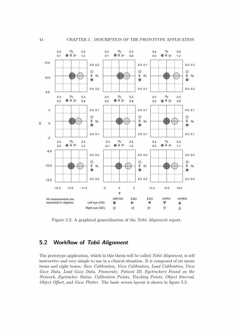
44 CHAPTER 5. DESCRIPTION OF THE PROTOTYPE APPLICATION
��� �
�
�
��
����� � �� �� � �� �
���
���
��� ���
���
���
��� ���
���
���
��� ���
���
���
��� ���
���
���
��� ���
���
���
��� ���
���
���
��� ���
���
���
���� ���
���
���
��� ���
��������������������
���� ������������������ �����
�����
����
�����
����
���
����
�� �����!�"��!�#����� $�%���&��'�()
�"#*���&��'�+()
, , ,
,
,
, ,
, ,
-
-
- - -
- -
- -
,
-
., ., .,
., ., .,
., ., .,
.- .- .-
.-.-.-
.- .- .-
��/ ��/ ��/ ��/
��/ ��/ ��/ ��/ ��/ ��/
��� ���
��� ��� ��� ������ ���
���
���
���
���
���
���
���
���
���
���
���
���
���
���
���
���
���
���
Figure 5.2: A graphical generalization of the Tobii Alignment report.
5.2 Workflow of Tobii Alignment
The prototype application, which in this thesis will be called Tobii Alignment, is selfinstructive and very simple to use in a clinical situation. It is composed of six menuitems and eight boxes: Save Calibration, View Calibration, Load Calibration, ViewGaze Data, Load Gaze Data, Framerate, Patient ID, Eyetrackers Found on theNetwork, Eyetracker Status, Calibration Points, Tracking Points, Object Interval,Object Offset, and Gaze Plotter. The basic screen layout is shown in figure 5.3.
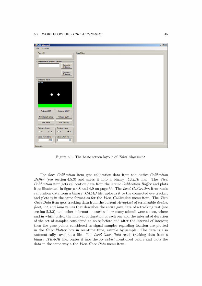
5.2. WORKFLOW OF TOBII ALIGNMENT 45
Figure 5.3: The basic screen layout of Tobii Alignment.
The Save Calibration item gets calibration data from the Active CalibrationBuffer (see section 4.5.3) and saves it into a binary .CALIB file. The ViewCalibration item gets calibration data from the Active Calibration Buffer and plotsit as illustrated in figures 4.8 and 4.9 on page 30. The Load Calibration item readscalibration data from a binary .CALIB file, uploads it to the connected eye tracker,and plots it in the same format as for the View Calibration menu item. The ViewGaze Data item gets tracking data from the current ArrayList of serializable double,float, int, and long values that describes the entire gaze data of a tracking test (seesection 5.2.2), and other information such as how many stimuli were shown, whereand in which order, the interval of duration of each one and the interval of durationof the set of samples considered as noise before and after the interval of interest;then the gaze points considered as signal samples regarding fixation are plottedin the Gaze Plotter box in real-time time, sample by sample. The data is alsoautomatically saved to a file. The Load Gaze Data reads tracking data from abinary .TRACK file, copies it into the ArrayList mentioned before and plots thedata in the same way a the View Gaze Data menu item.

46 CHAPTER 5. DESCRIPTION OF THE PROTOTYPE APPLICATION
The Patient ID box is where the patient’s identifier is entered. This identifier willbe used in conjunction with date, time, and type of calibration to name the calibra-tion, tracking, and report files. For example, if the patient ID is 33565791, the dateis October 6, 2012, the time is 12:34:56 and the tracking test is run after a monocularcalibration, the name of the files will be 33565791-20121006123456-monocular. Inthis way, comparing and following up the patient’s therapy is facilitated. This filename is generated when the binocular calibration is run or when both monocularcalibrations for the left and right eye are merged. The tracking and report files willhave the same root file name with the necessary number of suffixes if more than onetracking test is run for a given calibration.
The Eyetrackers Found on the Network box lists the eye trackers found on thenetwork. When an eyetracker is found on the network it is added to the list. Whenit disappears from the network it is removed from the list.
The Eyetracker Status box visualizes the position of the eyes. This is mainly atool to help the user position himself/herself in front of the tracker. This routineuses the relative eye position data from the left and right eye as explained insection 4.3 starting on page 22. This box also includes a set of six buttons as shownin figure 4.14 on page 40. The Calibrate LEFT and Calibrate RIGHT buttons runcalibrations, assuming that the specialist is occluding the patient’s right and lefteye with an IR light transparent lens respectively. Then the calibration is savedin memory. The calibrations of the left and right eye will be saved into .CALIBbinary files with the suffix “left” and “right” respectively when the user clicks onthe MERGE Calibrations button. This button calls an external .EXE applicationprovided by Tobii Technology which gets as input two .CALIB files, each one foreach eye, and returns as output a .CALIB file after merging both eye calibrationmodels. The file will be given a name in such a way it will be easily related to theinput. The Calibrate BOTH button runs a binocular calibration, assuming thatno IR light transparent lens is being used. Then the calibration is saved. TheHide/Show Status button disables/enables the Eyetracker Status box. The StartTracking button runs a tracking test (see section 5.2.2).
The Calibration Points and Tracking Points boxes let the user choose how manystimuli will be shown in the calibration and tracking procedures respectively. TheObject Interval and Object Offset boxes let the user decide the interval of durationof each of those objects and the interval of duration of the set of samples consideredas noise before and after the interval of interest.
The Gaze Plotter box is the most important one. After a tracking test is run, leftand right eye’s samples are plotted in red and green respectively in real-time. Thereare 9 cardinal positions similar those it is illustrated in figure 5.2. The percentage ofsamples that were validated is printed as well. It was agreed with the supervisor ofthis thesis project to remove the labels regarding ophthalmic disorders by allowingthe ophthalmologist to have the final say by observing the computed statistics. Anexample of the appearance of the Gaze Plotter is shown in figure 5.4.
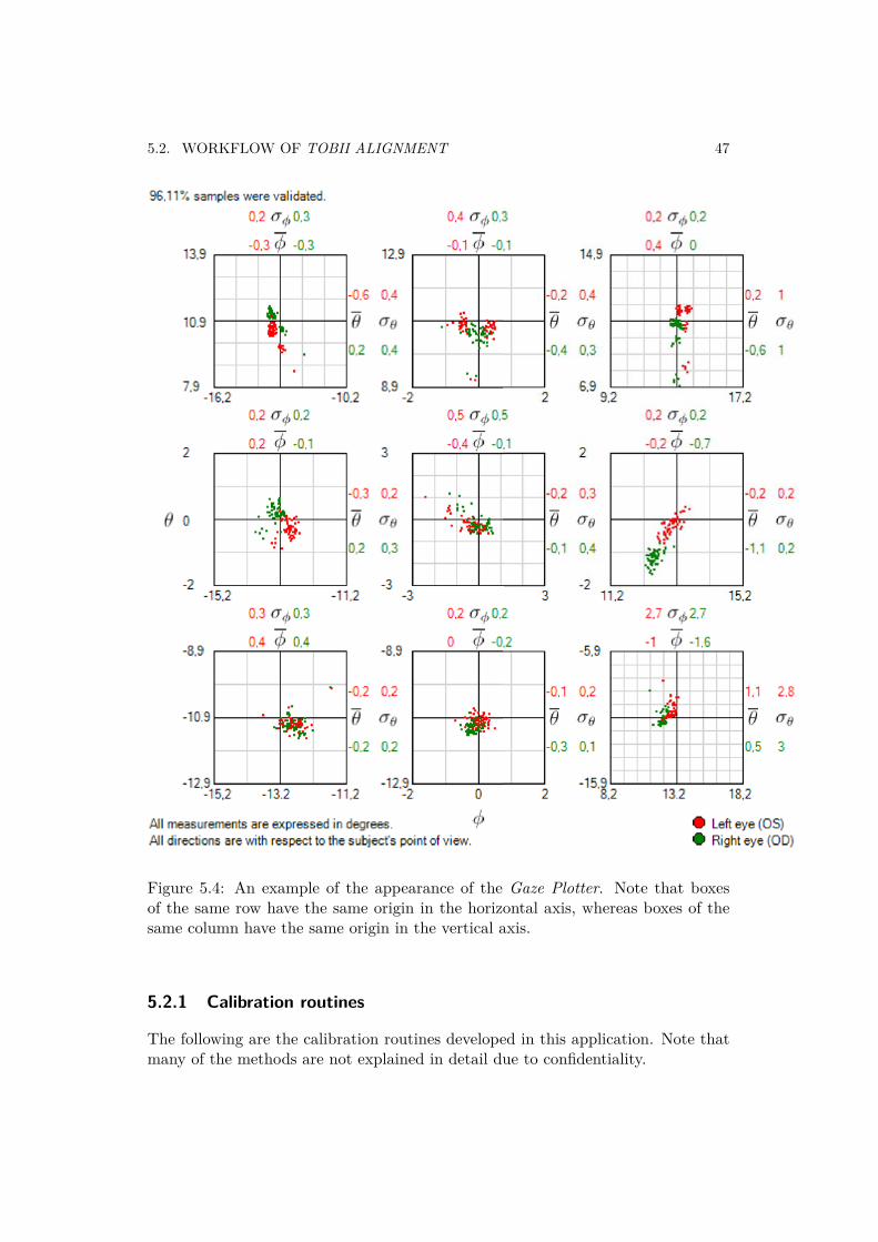
5.2. WORKFLOW OF TOBII ALIGNMENT 47
Figure 5.4: An example of the appearance of the Gaze Plotter. Note that boxesof the same row have the same origin in the horizontal axis, whereas boxes of thesame column have the same origin in the vertical axis.
5.2.1 Calibration routines
The following are the calibration routines developed in this application. Note thatmany of the methods are not explained in detail due to confidentiality.

48 CHAPTER 5. DESCRIPTION OF THE PROTOTYPE APPLICATION
Listing 5.1: The binocular calibration routinep r i v a t e void _calibrateBinocularButton_Click ( o b j e c t sender , EventArgs e ){
i f ( _isTracking ){
// Unsubscr ibe from gaze data stream_connectedTracker . StopTracking ( ) ;_isTracking = f a l s e ;
}UpdateUIElements ( ) ; // Update user i n t e r f a c e e lements
var runner = new Cal ibrat ionRunner ( ) ;
t ry{
// Star t a new c a l i b r a t i o n procedureC a l i b r a t i o n binocularCalibration = runner . RunCalibration (←↩
_connectedTracker , _howManyCalibrationPoints ) ;
// Show a c a l i b r a t i o n p lo t i f eve ryth ing went OKi f ( binocularCalibration != n u l l ){
// Save the c a l i b r a t i o n on the r i g h t eyebinocularFileName = participantTextBox1 . Text + ' − ' + ←↩
UpdateTodayNow ( ) + ' − ' + _howManyCalibrationPoints + "←↩points −b i n o c u l a r . c a l i b " ;
SaveCalibration ( binocularCalibration , binocularFileName ) ;
var resultForm = new Cal ibrat ionResultForm ( ) ;resultForm . SetPlotData ( binocularCalibration ) ;resultForm . Text = "BINOCULAR C a l i b r a t i o n Result " ;resultForm . ShowDialog ( ) ;loadedCalibration = " b i n o c u l a r " ;
}e l s e{
MessageBox . Show ( " Not enough data to c r e a t e a c a l i b r a t i o n ( or ←↩c a l i b r a t i o n aborted ) . " ) ;
}}catch ( EyetrackerExcept ion ee ){
MessageBox . Show ( " Fa i l ed to c a l i b r a t e . Got except ion " + ee ," C a l i b r a t i o n Fa i l ed " ,MessageBoxButtons . OK ,MessageBoxIcon . Error ) ;
}f i n a l l y{
rightCalibration = n u l l ;leftCalibration = n u l l ;
i f ( ! _isTracking ){
// Star t s u b s c r i b i n g to gaze data stream_connectedTracker . StartTracking ( ) ;_isTracking = true ;
}UpdateUIElements ( ) ; // Update user i n t e r f a c e e lements
}}

5.2. WORKFLOW OF TOBII ALIGNMENT 49
Listing 5.2: The monocular calibration on the left eye routinep r i v a t e void _calibrateLeftButton_Click ( o b j e c t sender , EventArgs e ){
// Hide the c u r s o r when the mouse p o i n t e r e n t e r s the button .Cursor . Hide ( ) ;
i f ( _isTracking ){
// Unsubscr ibe from gaze data stream_connectedTracker . StopTracking ( ) ;_isTracking = f a l s e ;
}UpdateUIElements ( ) ; // Update user i n t e r f a c e e lements
var runner = new Cal ibrat ionRunner ( objectInterval ) ;
t ry{
// Star t a new c a l i b r a t i o n procedureleftCalibration = runner . RunCalibration ( _connectedTracker , ←↩
howManyCalibrationPoints ) ;
// Show a c a l i b r a t i o n p lo t i f eve ryth ing went OKi f ( leftCalibration != n u l l ){
var resultForm = new Cal ibrat ionResultForm ( ) ;resultForm . SetPlotData ( leftCalibration ) ;resultForm . Text = " Monocular C a l i b r a t i o n on the LEFT Eye Result←↩
" ;resultForm . ShowDialog ( ) ;loadedCalibration = n u l l ;
}e l s e{
MessageBox . Show ( " Not enough data to c r e a t e a c a l i b r a t i o n ( or ←↩c a l i b r a t i o n aborted ) . " ) ;
}}catch ( EyetrackerExcept ion ee ){
MessageBox . Show ( " Fa i l ed to c a l i b r a t e . Got except ion " + ee ," C a l i b r a t i o n Fa i l ed " ,MessageBoxButtons . OK ,MessageBoxIcon . Error ) ;
}f i n a l l y{
i f ( ! _isTracking ){
// Star t s u b s c r i b i n g to gaze data stream_connectedTracker . StartTracking ( ) ;_isTracking = true ;
}UpdateUIElements ( ) ; // Update user i n t e r f a c e e lements
// Show the c u r s o r when the mouse p o i n t e r l e a v e s the button .Cursor . Show ( ) ;
}}

50 CHAPTER 5. DESCRIPTION OF THE PROTOTYPE APPLICATION
Listing 5.3: The monocular calibration on the right eye routinep r i v a t e void _calibrateRightButton_Click ( o b j e c t sender , EventArgs e ){
i f ( _isTracking ){
// Unsubscr ibe from gaze data stream_connectedTracker . StopTracking ( ) ;_isTracking = f a l s e ;
}UpdateUIElements ( ) ; // Update user i n t e r f a c e e lements
var runner = new Cal ibrat ionRunner ( ) ;
t ry{
// Star t a new c a l i b r a t i o n procedurerightCalibration = runner . RunCalibration ( _connectedTracker , ←↩
_howManyCalibrationPoints ) ;
// Show a c a l i b r a t i o n p lo t i f eve ryth ing went OKi f ( rightCalibration != n u l l ){
var resultForm = new Cal ibrat ionResultForm ( ) ;resultForm . SetPlotData ( rightCalibration ) ;resultForm . Text = " Monocular C a l i b r a t i o n on the RIGHT Eye ←↩
Result " ;resultForm . ShowDialog ( ) ;loadedCalibration = n u l l ;
}e l s e{
MessageBox . Show ( " Not enough data to c r e a t e a c a l i b r a t i o n ( or ←↩c a l i b r a t i o n aborted ) . " ) ;
}}catch ( EyetrackerExcept ion ee ){
MessageBox . Show ( " Fa i l ed to c a l i b r a t e . Got except ion " + ee ," C a l i b r a t i o n Fa i l ed " ,MessageBoxButtons . OK ,MessageBoxIcon . Error ) ;
}f i n a l l y{
i f ( ! _isTracking ){
// Star t s u b s c r i b i n g to gaze data stream_connectedTracker . StartTracking ( ) ;_isTracking = true ;
}UpdateUIElements ( ) ; // Update user i n t e r f a c e e lements
}}
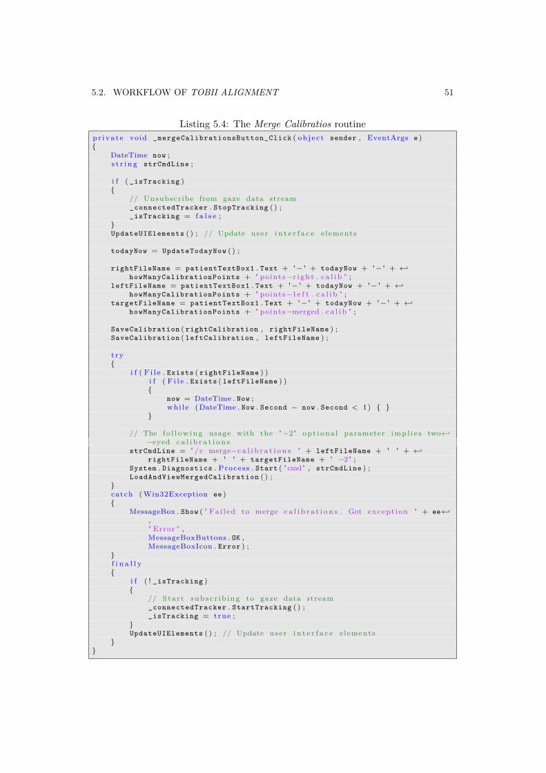
5.2. WORKFLOW OF TOBII ALIGNMENT 51
Listing 5.4: The Merge Calibratios routinep r i v a t e void _mergeCalibrationsButton_Click ( o b j e c t sender , EventArgs e ){
DateTime now ;s t r i n g strCmdLine ;
i f ( _isTracking ){
// Unsubscr ibe from gaze data stream_connectedTracker . StopTracking ( ) ;_isTracking = f a l s e ;
}UpdateUIElements ( ) ; // Update user i n t e r f a c e e lements
todayNow = UpdateTodayNow ( ) ;
rightFileName = patientTextBox1 . Text + ' − ' + todayNow + ' − ' + ←↩howManyCalibrationPoints + " points −r i g h t . c a l i b " ;
leftFileName = patientTextBox1 . Text + ' − ' + todayNow + ' − ' + ←↩howManyCalibrationPoints + " points − l e f t . c a l i b " ;
targetFileName = patientTextBox1 . Text + ' − ' + todayNow + ' − ' + ←↩howManyCalibrationPoints + " points −merged . c a l i b " ;
SaveCalibration ( rightCalibration , rightFileName ) ;SaveCalibration ( leftCalibration , leftFileName ) ;
t ry{
i f ( F i l e . Exists ( rightFileName ) )i f ( F i l e . Exists ( leftFileName ) ){
now = DateTime . Now ;whi l e ( DateTime . Now . Second − now . Second < 1) { }
}
// The f o l l o w i n g usage with the "−2" o p t i o n a l parameter i m p l i e s two←↩−eyed c a l i b r a t i o n s
strCmdLine = " /c merge−c a l i b r a t i o n s " + leftFileName + ' ' + ←↩rightFileName + ' ' + targetFileName + " −2" ;
System . Diagnostics . Process . Start ( "cmd" , strCmdLine ) ;LoadAndViewMergedCalibration ( ) ;
}catch ( Win32Exception ee ){
MessageBox . Show ( " Fa i l ed to merge c a l i b r a t i o n s . Got except ion " + ee←↩," Error " ,MessageBoxButtons . OK ,MessageBoxIcon . Error ) ;
}f i n a l l y{
i f ( ! _isTracking ){
// Star t s u b s c r i b i n g to gaze data stream_connectedTracker . StartTracking ( ) ;_isTracking = true ;
}UpdateUIElements ( ) ; // Update user i n t e r f a c e e lements
}}
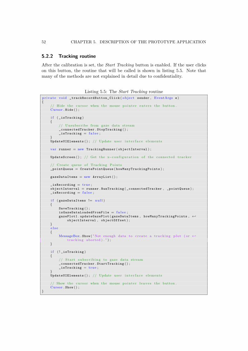
52 CHAPTER 5. DESCRIPTION OF THE PROTOTYPE APPLICATION
5.2.2 Tracking routineAfter the calibration is set, the Start Tracking button is enabled. If the user clickson this button, the routine that will be called is shown in listing 5.5. Note thatmany of the methods are not explained in detail due to confidentiality.
Listing 5.5: The Start Tracking routinep r i v a t e void _trackRecordButton_Click ( o b j e c t sender , EventArgs e ){
// Hide the c u r s o r when the mouse p o i n t e r e n t e r s the button .Cursor . Hide ( ) ;
i f ( _isTracking ){
// Unsubscr ibe from gaze data stream_connectedTracker . StopTracking ( ) ;_isTracking = f a l s e ;
}UpdateUIElements ( ) ; // Update user i n t e r f a c e e lements
var runner = new TrackingRunner ( objectInterval ) ;
UpdateScreen ( ) ; // Get the x−c o n f i g u r a t i o n o f the connected t r a c k e r
// Create queue o f Tracking Points_pointQueue = CreatePointQueue ( howManyTrackingPoints ) ;
gazeDataItems = new ArrayList ( ) ;
_isRecording = true ;objectInterval = runner . RunTracking ( _connectedTracker , _pointQueue ) ;_isRecording = f a l s e ;
i f ( gazeDataItems != n u l l ){
SaveTracking ( ) ;isGazeDataLoadedFromFile = f a l s e ;gazePlot1 . updateGazePlot ( gazeDataItems , howManyTrackingPoints , ←↩
objectInterval , objectOffset ) ;}e l s e{
MessageBox . Show ( " Not enough data to c r e a t e a t r a c k i n g p l o t ( or ←↩t r a c k i n g aborted ) . " ) ;
}
i f ( ! _isTracking ){
// Star t s u b s c r i b i n g to gaze data stream_connectedTracker . StartTracking ( ) ;_isTracking = true ;
}UpdateUIElements ( ) ; // Update user i n t e r f a c e e lements
// Show the c u r s o r when the mouse p o i n t e r l e a v e s the button .Cursor . Show ( ) ;
}

Chapter 6
Evaluation
This chapter contains the evaluation performed for the system architecture andprototype presented in chapter 5. Three different sets of tests were made. Animportant precaution regarding reliability is to measure all subjects with the samedevice and firmware for each study in order to avoid possible sources of variance.
6.1 Study I – Measurement of 2D gaze points on thetracking area
The purpose of this study was to measure relative gaze points of sixteen subjectsabove the age of 25 as a first concept of solution of the prototype application. Bothbinocular and monocular calibrations were conducted at Tobii Technology by usinga Tobii T60 Eye Tracker. The IR transparent lenses mentioned on page 17 wereused to conduct monocular calibration.
It turned out that crossed fixations1 were obtained at distances of between 60and 65 cm. For binocular calibration crossed fixations of larger than 40 pixels2were observed in 18.7% of the objects across all of the objects shown to the sixteensubjects. For monocular calibration by using a 750 nm wavelength IR transparentlens the percentage was 38.6%. For monocular calibration by using a 800 nmwavelength IR transparent lens crossed fixations of larger than 40 pixels on thetracking plane were collected in 45.6% of the objects across all of the objects shownto the sixteen subjects as well.
Figures 6.1, 6.2, and 6.3 show examples of crossed fixations obtained from750 nm monocular, 800 nm monocular, and binocular calibrations for subjects #4,#11, and #10 respectively.
1A crossed fixation occurs when the left eye is located further to the right than the right eye.2A segment of 40 pixels long on the diagonal of a 17-inch monitor with a resolution of
1280 × 1024 pixels observed from a point that is 60 cm straightly in front of the screen describesan angle of 1o. This threshold of 1o could discard crossed fixations since it is of the same order ofmagnitude as a microsaccade [18].
53

54 CHAPTER 6. EVALUATION
Figure 6.1: Monocular calibration on subject #4 with 750 nm wavelength IRtransparent lens.
Figure 6.2: Monocular calibration on subject #11 with 800 nm wavelength IRtransparent lens.

6.1. STUDY I – MEASUREMENT OF 2D GAZE POINTS ON THE TRACKINGAREA 55
Figure 6.3: Binocular calibration on subject #10.
These results show that the 750 nm wavelength IR transparent lens producesbetter results than the 800 nm IR transparent lens. This can be reasonable since atypical human eye will respond to wavelengths from about 390 to 750 nm althoughsome people may be able to perceive wavelengths from 380 to 780 nm [8]. Thus,some of the sixteen subjects who had participated in this study may have fixatedunconsciously with the eye occluded by the 750 nm wavelength IR transparent lensas well as the not occluded eye. This might be why the results obtained after750 nm monocular calibration are more similar to the obtained after binocularcalibration (without any IR transparent lens) than the obtained after 800 nmmonocular calibration.
This observation motivated a series of tests using VOG with monocularcalibration, which has been performed by researchers at Bernadottelaboratoriet atS:t Eriks Ögonsjukhus. Crossed fixations at distances of between 60 and 65 cmwere obtained there as well (these tests are not included in this report). The resultsfrom the VOG looked very much like the results from the round of tests that I haveconducted with the Tobii T60 Eye Tracker in Study I.
This finding matched the results expected from [17]. Binocular eye movementsof normal adult readers were examined as they read single sentences by AntjeNuthmann and Reinhold Kliegl in this work. Analyses of horizontal and verticalfixation disparities carried out in Nuthmann’s and Kliegl’s work indicated that themost prevalent type of disparate fixation were crossed as well.

56 CHAPTER 6. EVALUATION
Either the distance to the display of the Tobii T60 Eye Tracker or that a displayis used affect the results. This motivated studies II & III.
6.2 Study II – Measurement of angles of deviationbetween gaze and target vectors
The study II has been carried out after implementing a new version of the prototypeapplication. This phase of testing included calculation of angle of deviation (as wasexplained in section 5.1). The purpose of this study was to measure gaze deviationsof twelve subjects above the age of 25 using a second version of the prototypeapplication. Both binocular and monocular calibrations were conducted at TobiiTechnology by using a Tobii T60 Eye Tracker. A 750 nm wavelength IR transparentlens provided by production staff working at Tobii Technology was used to occludethe subject’s corresponding eye since this lens performed better than the 800 nmwavelength lens did in the study I (see section 6.1).
In this study eighteen tracking tests were performed on every subject. Thetests were divided into two rounds that took place on two different days and atdifferent times (one round in the morning, one round in the afternoon). Eachround consisted of nine tracking tests: three tests after a binocular calibration,three tests after a monocular calibration run first on the left eye (MONO LR), andthree tests after a monocular calibration run first on the right eye (MONO RL).For the first round, the MONO LR procedure was performed first, followed by theMONO RL procedure. For the second round, the order of the monocular calibrationwas reversed. In this way, repeatability and independence of results obtained afterdifferent combinations of procedures at different times were analyzed and evaluated.
Figures 6.4 to 6.7 show average deviation with respect to the correspondingtarget point for every subject, calibration, session, and test. Looking at these figures,the reader may see that many tests produced similar results when replicated on agiven subject. Thus, there is a good grade of repeatability and independence forevery pair of sessions.
Figure 6.8 shows the average vergence angle values for every subject, calibration,session, and test. Looking at this figure, the reader may see that most of the vergenceangle values are negative. Since the origin is the vertical axis of the correspondingtarget point, when we have φL − φR < 0, there is uncrossed fixation on averageacross all of the objects shown for each subject for the corresponding calibration,what implies that uncrossed fixations were more frequent than crossed fixations.

6.2. STUDY II – MEASUREMENT OF ANGLES OF DEVIATION BETWEEN GAZEAND TARGET VECTORS 57
� � � � � � � � � �
� ��� ���� ��� ��� �� �� ��
�����
�������
(a) Binocular calibration, session #1.
� � � � � � � � �
� ��� ���� ��� ��� �� �� ��
�����
�������
(b) Binocular calibration, session #2.
� � � � � � � � �
�� ��� ��� ���� ��� ��� �� �� ��� ��
�����
�������
(c) MONO LR calibration, session #1.
� � � � � � � � �
�� ��� ��� ���� ��� ��� �� �� ��� ��
�����
�������
(d) MONO LR calibration, session #2.
� � � � � � � � �
�� ��� ��� ���� ��� ��� �� �� ��� ��
�����
�������
(e) MONO RL calibration, session #1.
� � � � � � � � �
�� ��� ��� ���� ��� ��� �� �� ��� ��
�����
�������
(f) MONO RL calibration, session #2.
Figure 6.4: Average φL deviations for every subject, calibration, session, and test.All measurements are expressed in degrees. Note that the plots of binocularcalibration are scaled to a different range.

58 CHAPTER 6. EVALUATION
� � � � � � � � �
� ��� ���� ��� ��� �� �� ��
�����
�������
(a) Binocular calibration, session #1.
� � � � � � � � �
� ��� ���� ��� ��� �� �� ��
�����
�������
(b) Binocular calibration, session #2.
� � � � � � � � �
�� ��� ��� ���� ��� ��� �� �� ��� ��
�����
�������
(c) MONO LR calibration, session #1.
� � � � � � � � �
�� ��� ��� ���� ��� ��� �� �� ��� ��
�����
�������
(d) MONO LR calibration, session #2.
� � � � � � � � �
�� ��� ��� ���� ��� ��� �� �� ��� ��
�����
�������
(e) MONO RL calibration, session #1.
� � � � � � � � �
�� ��� ��� ���� ��� ��� �� �� ��� ��
�����
�������
(f) MONO RL calibration, session #2.
Figure 6.5: Average θL deviations for every subject, calibration, session, and test.All measurements are expressed in degrees. Note that the plots of binocularcalibration are scaled to a different range.

6.2. STUDY II – MEASUREMENT OF ANGLES OF DEVIATION BETWEEN GAZEAND TARGET VECTORS 59
� � � � � � � � �
� ��� ���� ��� ��� �� �� ��
�����
�������
(a) Binocular calibration, session #1.
� � � � � � � � �
� ��� ���� ��� ��� �� �� ��
�����
�������
(b) Binocular calibration, session #2.
� � � � � � � � �
�� ��� ��� ���� ��� ��� �� �� ��� ��
�����
�������
(c) MONO LR calibration, session #1.
� � � � � � � � �
�� ��� ��� ���� ��� ��� �� �� ��� ��
�����
�������
(d) MONO LR calibration, session #2.
� � � � � � � � �
�� ��� ��� ���� ��� ��� �� �� ��� ��
�����
�������
(e) MONO RL calibration, session #1.
� � � � � � � � �
�� ��� ��� ���� ��� ��� �� �� ��� ��
�����
�������
(f) MONO RL calibration, session #2.
Figure 6.6: Average φR deviations for every subject, calibration, session, and test.All measurements are expressed in degrees. Note that the plots of binocularcalibration are scaled to a different range.

60 CHAPTER 6. EVALUATION
� � � � � � � � �
� ��� ���� ��� ��� �� �� ��
�����
�������
(a) Binocular calibration, session #1.
� � � � � � � � �
� ��� ���� ��� ��� �� �� ��
�����
�������
(b) Binocular calibration, session #2.
� � � � � � � � �
�� ��� ��� ���� ��� ��� �� �� ��� ��
�����
�������
(c) MONO LR calibration, session #1.
� � � � � � � � �
�� ��� ��� ���� ��� ��� �� �� ��� ��
�����
�������
(d) MONO LR calibration, session #2.
� � � � � � � � �
�� ��� ��� ���� ��� ��� �� �� ��� ��
�����
�������
(e) MONO RL calibration, session #1.
� � � � � � � � �
�� ��� ��� ���� ��� ��� �� �� ��� ��
�����
�������
(f) MONO RL calibration, session #2.
Figure 6.7: Average θR deviations for every subject, calibration, session, and test.All measurements are expressed in degrees. Note that the plots of binocularcalibration are scaled to a different range.
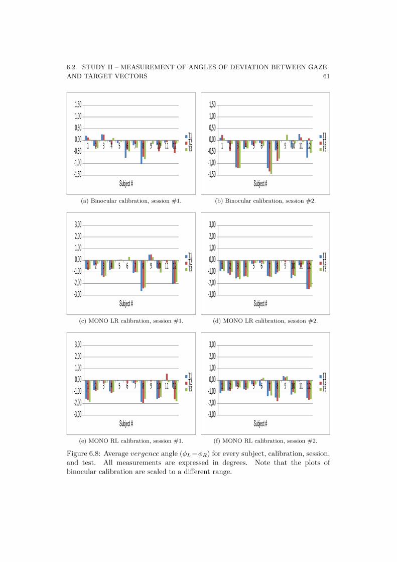
6.2. STUDY II – MEASUREMENT OF ANGLES OF DEVIATION BETWEEN GAZEAND TARGET VECTORS 61
� � � � � � � � �
� ��� ���� ��� ��� �� �� ��
�����
�������
(a) Binocular calibration, session #1.
� � � � � � � � �
� ��� ���� ��� ��� �� �� ��
�����
�������
(b) Binocular calibration, session #2.
� � � � � � � � �
�� ���� ��� ��� �� ��� ��� ��
�����
�������
(c) MONO LR calibration, session #1.
� � � � � � � � �
�� ���� ��� ��� �� ��� ��� ��
�����
�������
(d) MONO LR calibration, session #2.
� � � � � � � � �
�� ���� ��� ��� �� ��� ��� ��
�����
�������
(e) MONO RL calibration, session #1.
� � � � � � � � �
�� ���� ��� ��� �� ��� ��� ��
�����
�������
(f) MONO RL calibration, session #2.
Figure 6.8: Average vergence angle (φL −φR) for every subject, calibration, session,and test. All measurements are expressed in degrees. Note that the plots ofbinocular calibration are scaled to a different range.

62 CHAPTER 6. EVALUATION
However, the values shown before are the average of all the deviations withrespect to the corresponding target point for a given test. If we calculate theaverage of the deviations with respect to each target point separately between allthe subjects, then the crossed fixations are obtained as observed in the study I.This is why positive vergence angle values are obtained (see table 6.1).
Table 6.1: Mean and standard deviation values with respect to the correspondingtarget point for the nine cardinal positions and all the subjects. Values in red are outof the desired range (a deviation within the order of magnitude of a microsaccademay be ignored, and the implication of a positive vergence value is crossed fixation).
φL φR v θL θR σφL σφR σθL σθR
NW 0.3 -0.3 0.6 -0.7 -0.1 0.4 0.4 0.3 0.3N 0.3 -0.2 0.5 -0.5 -0.5 0.2 0.2 0.2 0.2NE 0.1 -0.2 0.3 -0.2 -0.7 0.2 0.2 0.2 0.2W 0.7 0.0 0.7 -0.5 0.0 0.2 0.2 0.2 0.2C 0.2 -0.5 0.7 -0.4 -0.4 0.2 0.2 0.3 0.2E -0.2 -0.8 0.6 -0.2 -0.6 0.2 0.2 0.2 0.2SW 1.0 0.3 1.3 0.1 0.4 0.4 0.4 0.3 0.3S 0.4 -0.6 1.0 0.1 0.3 0.4 0.3 0.1 0.3SE -0.5 -1.3 0.8 0.2 0.2 0.4 0.4 0.4 0.3
Figures 6.9, 6.10, and 6.11 show the linear regression for φL, φR, θL, and θR
for average results of binocular, MONO LR, and MONO RL calibrations in thetwo different sessions for all the subjects. In these figures, each blue dot representsthe average angle of deviation across all of the objects shown for each subject forthe corresponding calibration and variable. This offers a better approach to seehow valid the results are regarding repeatability and independence. Results showR2-values up to 0.7566.
These results in conjunction with the illustrated in figures 6.4 to 6.7 suggestthat there is a good grade of repeatability and independence of results obtainedafter different combinations of procedures at different times.

6.2. STUDY II – MEASUREMENT OF ANGLES OF DEVIATION BETWEEN GAZEAND TARGET VECTORS 63
(a) φL. (b) φR.
(c) θL. (d) θR.
Figure 6.9: Linear regression for binocular calibration. All measurements areexpressed in degrees.

64 CHAPTER 6. EVALUATION
(a) φL. (b) φR.
(c) θL. (d) θR.
Figure 6.10: Linear regression for MONO LR calibration. All measurements areexpressed in degrees.

6.2. STUDY II – MEASUREMENT OF ANGLES OF DEVIATION BETWEEN GAZEAND TARGET VECTORS 65
(a) φL. (b) φR.
(c) θL. (d) θR.
Figure 6.11: Linear regression for MONO RL calibration. All measurements areexpressed in degrees.

66 CHAPTER 6. EVALUATION
6.3 Study III – Tobii Alignment validation against scleralsearch coil technique
In the study III several scleral search coil experiments were conducted, wherea Tobii T120 Eye Tracker and the SSC were used simultaneously. The SSC isconsidered the gold standard in eye tracking, thus this experiment shows precislyhow close the results of the prototype appliction with the Tobii T120 Eye Trackeris to this gold standard.
This section describes the validation procedure carried out to compare thenew method with the SSC. Although, for this study, all angles of deviation wereexpressed with respect to the center of the screen instead of the correspondingtarget point (as were the angles of deviation in the earlier studies). Since theresults obtained in the study II show that the test results were independent ofthe different combinations of procedures conducted at different times, thus inStudy III only MONO LR calibration was run before each set of tracking tests.Before describing this procedure, the principles of operation of the SSC installedat Bernadottelaboratoriet at S:t Eriks Ögonsjukhus are detailed in the followingsubsection.
6.3.1 Principles of operation of a scleral search coil
The basic principles of the electromagnetic recording used in this measurementtechnique originate from research conducted in [22, p. 137–145] and later in [25, p.447–450]. A small induction coil, with N turns, is embedded in a flexible ring ofsilicone rubber which adheres to the limbus (the border of the cornea and the sclera)of the adult human eye. Around the head of the subject an alternating horizontalHx and vertical Hy magnetic field is generated and consequently an alternatingvoltage Ei will be induced in the coil in accordance with Faraday’s law:
Ei = −dΨdt
(6.1)
If all turns contain the same flux (φ) we find with the coupled flux:
Ψ =N∑
k=1φk (6.2)
that:
Ei = −N · dφ
dt(6.3)

6.3. STUDY III – TOBII ALIGNMENT VALIDATION AGAINST SCLERAL SEARCHCOIL TECHNIQUE 67
Flux is represented by:
φA =∫
AμH · dA. (6.4)
In which μ is the absolute permeability (μ = μ0μr) and Hn is the magneticinduction component perpendicular to the total area of A.
In case of a homogeneus magnetic field equation 6.4 becomes:
φ = μH · A (6.5)
When the eye looks up by the angle θ and the vertical magnetic field intensityis given by Hv = H cosωt, then the induced voltage for this vertical position willbe:
Ei = ωNAμH sin θ sinωt (6.6)
Before we add a second coil to these considerations we define appropriate anglesin a coordinate system. We consider a sphere comparable with the terrestrial globe.The eye is positioned in the centre and looking in the direction of the intersectionbetween the earth’s equator and the 0o meridian Greenwich.
The axes of rotation are taken as follow:
x-axis• : 90o West longitude to 90o East longitude.
y-axis• : North to South.
z-axis• : 0o longitude to 180o longitude.
As a result of these assumptions the primary positions of the horizontal/verticalcoils are in parallel with respectively the x−y and y−z plane. Horizontal deflectioncan thus be described as a rotation of φ degrees about the y-axis. For a verticaldeflection we find a rotation of respectively θ degrees about the x-axis.
When we use two magnetic fields spatially and temporally in quadrature andtwo lens coils in spatial quadrature, it is easy to deduce that:

68 CHAPTER 6. EVALUATION
1. Position of the axis of rotation for vertical deflection changes with horizontaldeflection.
2. Position of the axis of rotation for horizontal deflection does not change withvertical deflection.
These deductions lead to two DC signals:
Eφ ∝ sinφ cos θ (6.7)
Eθ ∝ sin θ (6.8)
If φ and θ are all less than 20o, sinφ departs from φ in radians by less than 2%and cos θ departs from unity by less than 6% so that approximately:
Eφ ∝ φ (6.9)
Eθ ∝ θ (6.10)
The coil-frame is a cube (70x70x70 cm) in which six coils are embedded. Eachcoil is individually shielded with copper shielding tape. In this way the electricfield, which is generated at the same time as the magnetic field, is considerablyreduced. The left and right coils generate a horizontal magnetic field, while thetop and bottom coils generate a vertical magnetic field. The current through thehorizontal coils is a sine waveform, while the current through the vertical coils isa cosine waveform. Both current values are identical (325 mA rms) and both havethe same frequency (20 kHz).
For easy calibration, the coil-frame is supplied with a third set of coils. Thecurrent through these coils corresponds to an eye deflection of 10o. The actualvalue is 325 times the sine of 10o, which is 56.4 mA (rms).
A calibration signal, equivalent to 10 degrees eye deflection, is obtained bypressing the calibration button. Pressing the H-calibration button will induce asine waveform magnetic field, while pressing the V-calibration button will induce acosine waveform magnetic field.
With the aid of a calibration device, capable of simulating horizontal and verticalposition a registration of a calibration is recorded. A current with a value equalto the sine of 10o times the regular current (325 mA rms) is fed to the calibrationmagnet coils located in front and at the back of the SSC. The SSC is thus energizedby the calibration magnetic field perpendicular to this coil. Whether the coil isnot exactly perpendicular to this calibration magnetic field does not influence this

6.3. STUDY III – TOBII ALIGNMENT VALIDATION AGAINST SCLERAL SEARCHCOIL TECHNIQUE 69
calibration technique much. When for example the primary position of the coil is5o to the right the induced voltage will only be 0.4% less (cosine 5o = 0.996).
6.3.2 Validation procedure
Two tables of events were designed by Gustaf Öqvist Seimyr, the supervisor of thisthesis project, in order to study a comparison between the SSC and the Tobii T120Eye Tracker performance for both binocular and monocular calibrations. Theseevents are listed in tables 6.2 and 6.3.
Table 6.2: Binocular calibration procedure in a SSC setting.
Event Duration (s) Time (ms)Start SSC recording 0 0View far center target (600 cm) 10 10000Horizontal and vertical SSC calibration signal 5 15000Place Tobii T120 Eye Tracker in front of the subject 15 30000View near center target (60 cm) 10 40000Run binocular calibration 30 70000Run tracking test three times 90 160000Stop SSC recording 0 160000
Table 6.3: Monocular calibration procedure in a SSC setting.
Event Duration (s) Time (ms)Start SSC recording 0 0View far center target (600 cm) 10 10000Horizontal and vertical SSC calibration signal 5 15000Place Tobii T120 Eye Tracker in front of the subject 15 30000View near center target (60 cm) 10 40000Calibrate left eye (OS) 30 70000Calibrate right eye (OD) 30 100000Run tracking test three times 90 190000Stop SSC recording 0 190000
After all the assumptions made in section 6.3.1, it is possible to calculate allthe angles of deviation values from the text file returned by an application whichrecords the voltage values at a framerate of 1 kHz for both the left and right eyefrom the SSC system. In that text file, voltage values are organized in a matrix insuch a way the first column is the time stamp in seconds with a precision of 1 ms,the second and third columns are the right eye’s horizontal and vertical deflection

70 CHAPTER 6. EVALUATION
voltages respectively, and the fourth and fifth columns are the left eye’s horizontaland vertical deflection voltages respectively. There are as many rows as samples.
6.3.3 Transformation from voltage to angle of deviationTo transform the voltage values to angle of deviation values, the maximum absolutevalue for each voltage column for rows from samples 10001 to 15000 (see tables6.2 and 6.3) which corresponds with an eye deflection of 10o is found. This valuecorresponds to the event when the volunteer was looking at the far center targetpoint, and the calibration button was pressed to obtain the calibration signal. Then,all the voltage values of each column are divided by their corresponding maximumabsolute values and finally multiplied by 10o. In this way, all values are transformedto angle of deviation expressed with respect to the vector from the eye’s position tothe far center target point (far center target vector).
In order to avoid considering a peak voltage value as maximum, we utilize themaximum of the mean of all voltage values for half a second (i.e., 500 ms) after theactual maximum. This can be easily done by finding the actual absolute maximumvalue for each column and calculating the maximum of the mean. After thesecalculations, all the voltage values of each column of the original matrix are dividedby their corresponding “maximum” absolute values and finally multiplied by 10o.In this way, all values are transformed to angle of deviation while avoiding theinfluence of a peak voltage value.
In addition, all the angle of deviation values have to be subtracted from theexisting offsets. These offsets can be approximated as the average values of theangles of deviation when the volunteer is looking at the near center target for 2.2seconds. Note that the volunteer is aware of the duration of the objects that areshown on the screen during the tests. Thus, the offsets are the average of the valuesfor each angle of deviation column for rows 30001 to 32200 (see tables 6.2 and 6.3).Listing 6.1 shows how “maximum” values were calculated and how the offset issubtracted by using MATLAB.
Listing 6.1: Transformation from voltage to angle of deviation.f u n c t i o n angleData = transformer ( voltageData )% angleData = trans fo rmer ( voltageData )% voltageData : " time ( sec ) " , "RE Hor " , "RE Ver " , "LE Hor " , "LE Ver "
% Actual maximum v o l tage va lue s f o r the c a l i b r a t i o n i n t e r v a lmaximum = max( abs ( voltageData ( 1 0 0 0 1 : 1 5 0 0 0 , : ) ) ) ;% Get the indexes o f the a c t u a l maximum v o l t a g e v a l u e smaxIndex2 = f i n d ( abs ( voltageData (10001 :15000 ,2 ) ) == maximum (2 ) ) ;maxIndex3 = f i n d ( abs ( voltageData (10001 :15000 ,3 ) ) == maximum (3 ) ) ;maxIndex4 = f i n d ( abs ( voltageData (10001 :15000 ,4 ) ) == maximum (4 ) ) ;maxIndex5 = f i n d ( abs ( voltageData (10001 :15000 ,5 ) ) == maximum (5 ) ) ;% Let them be the maximum va lue s the mean o f a l l v o l tage va lue s f o r h a l f a% second a f t e r the a c t u a l maximum f o r each columnmaximum (2 ) = mean( voltageData ( maxIndex2 +10001: maxIndex2 +10100 ,2) ) ;maximum (3 ) = mean( voltageData ( maxIndex3 +10001: maxIndex3 +10100 ,3) ) ;

6.3. STUDY III – TOBII ALIGNMENT VALIDATION AGAINST SCLERAL SEARCHCOIL TECHNIQUE 71
maximum (4 ) = mean( voltageData ( maxIndex4 +10001: maxIndex4 +10100 ,4) ) ;maximum (5 ) = mean( voltageData ( maxIndex5 +10001: maxIndex5 +10100 ,5) ) ;
angleData ( : , 1 ) = voltageData ( : , 1 ) ; % Time ( seconds )% Al l the vo l tage va lue s o f each column are d iv ided by t h e i r cor re spond ing% "maximum" ab s o l u te va lue s and f i n a l l y m u l t i p l i e d by 10angleData ( : , 2 ) = voltageData ( : , 2 ) / maximum (2 ) ∗10 ;angleData ( : , 3 ) = voltageData ( : , 3 ) / maximum (3 ) ∗10 ;angleData ( : , 4 ) = voltageData ( : , 4 ) / maximum (4 ) ∗10 ;angleData ( : , 5 ) = voltageData ( : , 5 ) / maximum (5 ) ∗10 ;% Al l the ang le va lue s o f each column are s u b s t r a c t e d each mean value% correspond ing to the f i x a t i o n at the near c e n t e r t a r g e t (60 cm)angleData ( : , 2 ) = angleData ( : , 2 ) − mean( angleData (30001 :32200 ,2 ) ) ;angleData ( : , 3 ) = angleData ( : , 3 ) − mean( angleData (30001 :32200 ,3 ) ) ;angleData ( : , 4 ) = angleData ( : , 4 ) − mean( angleData (30001 :32200 ,4 ) ) ;angleData ( : , 5 ) = angleData ( : , 5 ) − mean( angleData (30001 :32200 ,5 ) ) ;
6.3.4 Interpolation and decimation of a set of samplesAfter carrying out the transformation explained in the previous subsection, we mustdeal with a problem that often occurs in practice. Suppose that xi[n] is the set ofsamples returned by the SSC system, taken with a sampling frequency fSi. Weintend to find another set of samples xo[n] corresponding to the sampling of thesame analog signal with a sampling frequency fSo equal to the framerate of theTobii T120 Eye Tracker.
We address the problem by studying the case where fSo = (L/M) fSi, whereL and M are integers, i.e., there is a rational relationship between the samplingfrequencies. As fSi = 1000 Hz and fSo = 120 Hz, L/M = 3/25 < 1. Thus, we talkabout decimating by a rational factor.
It is easy to see that concatenating an interpolation and decimation by integerfactors L and M respectively the desired goal is achieved. There might be a questionof which should be done first: interpolation or decimation. To answer this questionwe must remember that decimation destroys information. For this reason it isnecessary to first perform interpolation and then decimation.
To interpolate a signal it is padded with zeros and low-pass filtered with animpulse response shaped filter [39, p. 23]:
h[n] = sincn
L(6.11)
This filter is ideal and, therefore, unfeasible. As a result it is necessary toapproximate an impulse response. A commonly used filter is the linear interpolator.It is known by this name because the new samples are calculated by drawing straightlines between the neighboring values. Listing 6.2 shows the calculations of theinterpolated samples as implemented in MATLAB R2010b.

72 CHAPTER 6. EVALUATION
Listing 6.2: Linear interpolation.f u n c t i o n x2 = interpolator ( x1 , L )% x2 = i n t e r p o l a t o r ( x1 , L)% x1 : s e t o f samples to i n t e r p o l a t e .% L : f a c t o r o f i n t e r p o l a t i o n .
x2 = x1 ( 1 , : ) ; % The f i r s t sample o f each column o f x1 i s takenf o r i = 1 : l ength ( x1 )−1
% For each p a i r o f samples , c a l c u l a t e the s l o p e o f the l i n e they% d e s c r i b em ( 1 , : ) = ( x1 ( i +1 , :) − x1 ( i , : ) ) . / L ;% I n t e r p o l a t e with as many samples as L?1f o r j = 1 : L−1
x2 = [ x2j . ∗ m ( 1 , : )+x1 ( i , : ) ] ;
endx2 = [ x2
x1 ( i +1 , :) ] ; % Add the next sample o f x1end
An example for L = 3 is illustrated in figure 6.12. The reader might ask whatrelationship exists between this interpolation and ideal low-pass filter. The answeris that linear interpolation is equivalent to a zero padding followed by a triangularimpulse response filter, as shown in figure 6.13.
�� �� �� � � � ��
� � �
�
������
� � � � � �
� �
���������������� �
�
���������������
��������
Figure 6.12: Relationship between samples in a linear interpolator for L = 3.
It is known from the literature that when the signal is sufficiently sampled (i.e.,at least twice the Nyquist rate), the linear interpolator is a good approximation tothe ideal low-pass interpolation.

6.3. STUDY III – TOBII ALIGNMENT VALIDATION AGAINST SCLERAL SEARCHCOIL TECHNIQUE 73
�� �� � � �
����
�
���
����
� ��� �
Figure 6.13: Impulse response of a linear interpolator for L = 3.
If the final sampling frequency is M times smaller than fSo = L · fSi, i.e.:
fSo =L · fSi
M=
fSinterpolated
M(6.12)
Decimation is relatively simple. It will be sufficient to take one out of every Msamples of the interpolated input signal and copy them into the final output, i.e.,the system with the following input/output relationship will compute:
xo[n] = xinterpolated[Mn] (6.13)
Listing 6.3 shows the calculations of the new sampling that were implementedin MATLAB R2010b. Figure 6.14 shows the effect of a sampler for M = 8.
Listing 6.3: Sampling.f u n c t i o n x2 = sampler ( x1 , M )% x2 = sampler ( x1 , M)% x1 : s e t o f samples to decimate .% M: f a c t o r o f sampling .
x2 = [ ] ;
% Take one out o f every M samples o f the i n t e r p o l a t e d input s i g n a l and copy% them i n t o the f i n a l output .f o r i = 1 : M : l ength ( x1 )
x2 = [ x2x1 ( i , : ) ] ;
end
Thus, if we perform interpolation for L = 3 and then decimation for M = 25 tothe set of samples xi[n] with a sampling frequency fSi = 1000 Hz, the resulting setof samples xo[n] corresponds to sampling the same analog signal with a samplingfrequency fSo = 120 Hz.

74 CHAPTER 6. EVALUATION
�� �� �� � � � ��
�� �� �� � � � ��
�� �� �� �� �� �� � �� � � � � � � �
� �
� �
�
�
���������
���������������
Figure 6.14: Effect of a sampler for M = 8.
6.3.5 Correlation between the Tobii T120 Eye Tracker and SSCperformances
To figure out how the Tobii T120 Eye Tracker performs when compared with thegold standard, a correlation between tracking test data sets and their correspondingSSC sampled and transformed outputs in time was calculated.
After transforming the SSC data set in such a way that its values describeangles of deviation, it was necessary to look for synchronization points in both datasets. The synchronization must be done before the decimation, otherwise therewill be a phase error. This is a hard task since the validation procedure explainedin section 6.3.2 was manual and not that precise.
Interpolations for L = 3 to the set of samples from the SSC and L = 25 tothe set of samples from the Tobii T120 Eye Tracker were performed. Thus, sets ofsamples with a sampling frequency fSo = 3000 Hz were obtained.
Let x and y be two digital signals with the same sampling frequency and Nsamples each. The correlation in the changes in these two signals is calculated as:
rxy =
N∑i=1
(xi − x) · (yi − y)√√√√ N∑
i=1(xi − x)2 ·
√√√√ N∑i=1
(yi − y)2(6.14)
Listing 6.4 shows how the correlation in the changes in these signals with asampling frequency fS = 3000 Hz and their best corresponding indexes in the sets

6.3. STUDY III – TOBII ALIGNMENT VALIDATION AGAINST SCLERAL SEARCHCOIL TECHNIQUE 75
of samples were determined. In this way, it is possible to see which is the bestindex to use as a start offset to get the correlation value closest to 1.0, so that bothsets can be plotted in the same figure after sampling for M = 25. We considerthe best start offset as the average of the individual corresponding starting offsetsfor the left and right eye, with both horizontal and vertical deviations. This scriptalso calculates the ratio of valid samples returned by the Tobii T120 Eye Tracker.Listing 6.5 implements equation 6.14 on page 74 for the set of samples of the SSCsynchronized with samples from the Tobii T120 Eye Tracker as explained before.Listing 6.6 calculates the average of the set of samples discarding the invalid samplesreturned by the Tobii T120 Eye Tracker.
Listing 6.4: Correlation in the changes in the signals.f u n c t i o n [ r , index , sscRatio , tobiiRatio , best , bestIndex ] = ←↩
bestCorrelation ( ssc , tobii , start )% [ r , index , sscRat io , t o b i i R a t i o , best , best Index ] = b e s t C o r r e l a t i o n ( ssc , ←↩
t o b i i , s t a r t )
[ rows , columns ] = s i z e ( ssc ) ;r0 = −1∗ones (1 , columns −1) ;index0 = ones (1 , columns −1) ;sscRatio0 = z e r o s (1 , columns −1) ;tobiiRatio0 = z e r o s (1 , columns −1) ;ssc = transformer ( ssc ) ;ssc = ssc ( start : start +9∗2200+1000 ,:) ;tobii = interpolator ( tobii , 2 5 ) ;
f o r j = 2 : columnssscJ = interpolator ( ssc ( : , j ) , 3 ) ;f o r i = 1 : l ength ( sscJ )−l ength ( tobii )+1
[ r , sscRatio , tobiiRatio ] = correlator ( sscJ ( i : i+length ( tobii ) −1) ,←↩tobii ( : , j ) ) ;
i f r > r0 ( j−1)r0 ( j−1) = r ;index0 ( j−1) = i ;sscRatio0 ( j−1) = sscRatio ;tobiiRatio0 ( j−1) = tobiiRatio ;end
endend
r = r0 ;index = index0 ;sscRatio = sscRatio0 ;tobiiRatio = tobiiRatio0 ;best = [ start round (sum( r . ∗ index ) /sum( r ) ) ] ; bestIndex = sum( best ) ;

76 CHAPTER 6. EVALUATION
Listing 6.5: Calculation of the correlation in the changes in two signals.f u n c t i o n [ r , sscRatio , tobiiRatio ] = correlator ( ssc , tobii )% [ r , s scRat io , t o b i i R a t i o ] = c o r r e l a t o r ( ssc , t o b i i )% r : sample c o r r e l a t i o n c o e f f i c i e n t% sscRat io : percentage o f v a l i d samples in the s s c data s e t% t o b i i R a t i o : percentage o f v a l i d samples in the Tobi i data s e t
i f l ength ( ssc ) ~= length ( tobii )d i sp ( ' s s c and t o b i i have d i f f e r e n t s i z e ' )r = 0 ;sscRatio = 0 ;tobiiRatio = 0 ;re turn ;
end
sumNumerator = 0 ;sumXroot = 0 ;sumYroot = 0 ;[ sscmean , sscRatio ] = calcMean ( ssc ) ;[ tobiimean , tobiiRatio ] = calcMean ( tobii ) ;
f o r i = 1 : l ength ( ssc )i f i snan ( ssc ( i ) ) == 0 && isnan ( tobii ( i ) ) == 0
sumNumerator = sumNumerator + ( ssc ( i )−sscmean ) ∗( tobii ( i )−←↩tobiimean ) ;
sumXroot = sumXroot + ( ssc ( i )−sscmean ) ^2 ;sumYroot = sumYroot + ( tobii ( i )−tobiimean ) ^2 ;
endend
r = sumNumerator / ( s q r t ( sumXroot ) ∗ s q r t ( sumYroot ) ) ;
Listing 6.6: Calculation of the average discarding not valid samples.f u n c t i o n [ m , validityRatio ] = calcMean ( x )% [m, v a l i d i t y R a t i o ] = calcMean ( x )% m: mean o f x d i s c a r d i n g not v a l i d e lements% v a l i d i t y R a t i o : percentage o f v a l i d samples returned by the Tobi i Eye ←↩
Tracker
calcSum = 0 ;k = 0 ;
f o r i = 1 : l ength ( x )i f i snan ( x ( i ) ) == 0
calcSum = calcSum + x ( i ) ;k = k + 1 ;
endend
m = calcSum . / k ;validityRatio = k / l ength ( x ) ;
Correlation between both measurements for every volunteer, test, and variableare summarized in table 6.4 and illustrated in figure 6.15. All these correlationresults are over 0.9799 (the value in red), hence the reader may consider that thereis a very good correlation between both measurement techniques.

6.3. STUDY III – TOBII ALIGNMENT VALIDATION AGAINST SCLERAL SEARCHCOIL TECHNIQUE 77
Table 6.4: Correlation between both measurement techniques.
Subject # Test # rφL rφR rθL rθR
Binocular #11 0.9952 0.9937 0.9977 0.99302 0.9956 0.9934 0.9975 0.99343 0.9951 0.9918 0.9957 0.9913
Binocular #21 0.9945 0.9946 0.9971 0.99492 0.9951 0.9916 0.9925 0.99333 0.9967 0.9936 0.9960 0.9966
Monocular #11 0.9962 0.9927 0.9980 0.99312 0.9966 0.9931 0.9982 0.99403 0.9962 0.9930 0.9981 0.9944
Monocular #21 0.9959 0.9799 0.9882 0.99502 0.9974 0.9818 0.9890 0.99573 0.9968 0.9895 0.9900 0.9947
Figure 6.15: Correlation between both measurement techniques.
6.3.6 Graphical comparison between the Tobii T120 Eye Tracker andSSC performances
Figures from 6.16 to 6.25 show examples of graphical comparisons between theSSC and the eye tracker performances for every volunteer, calibration, and outputvariable. A comparison between calculations of vergence angle is included.
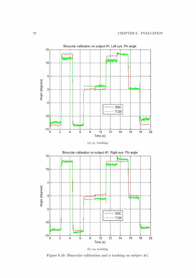
78 CHAPTER 6. EVALUATION
(a) φL tracking.
(b) φR tracking.
Figure 6.16: Binocular calibration and φ tracking on subject #1.

6.3. STUDY III – TOBII ALIGNMENT VALIDATION AGAINST SCLERAL SEARCHCOIL TECHNIQUE 79
(a) θL tracking.
(b) θR tracking.
Figure 6.17: Binocular calibration abd θ tracking on subject #1.

80 CHAPTER 6. EVALUATION
(a) φL tracking.
(b) φR tracking.
Figure 6.18: Monocular calibration and φ tracking on subject #1.

6.3. STUDY III – TOBII ALIGNMENT VALIDATION AGAINST SCLERAL SEARCHCOIL TECHNIQUE 81
(a) θL tracking.
(b) θR tracking.
Figure 6.19: Monocular calibration abd θ tracking on subject #1.

82 CHAPTER 6. EVALUATION
(a) Binocular calibration.
(b) Monocular calibration.
Figure 6.20: Vergence angle for subject #1.

6.3. STUDY III – TOBII ALIGNMENT VALIDATION AGAINST SCLERAL SEARCHCOIL TECHNIQUE 83
(a) φL tracking.
(b) φR tracking.
Figure 6.21: Binocular calibration and φ tracking on subject #2.
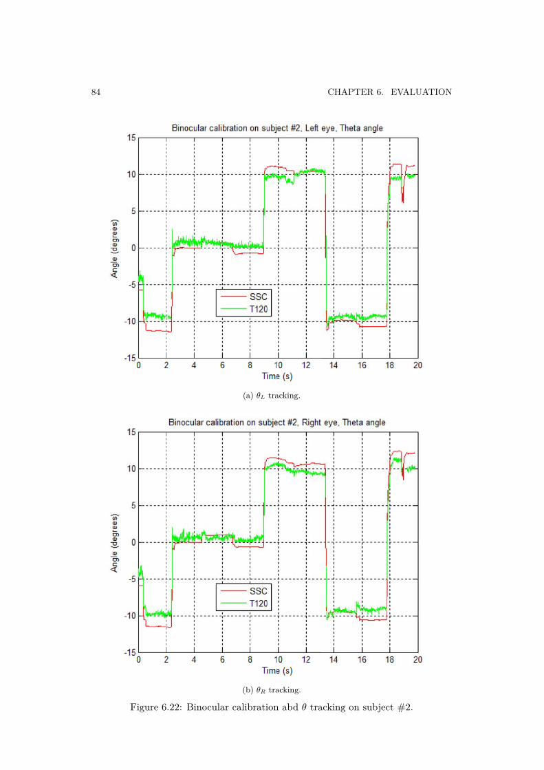
84 CHAPTER 6. EVALUATION
(a) θL tracking.
(b) θR tracking.
Figure 6.22: Binocular calibration abd θ tracking on subject #2.

6.3. STUDY III – TOBII ALIGNMENT VALIDATION AGAINST SCLERAL SEARCHCOIL TECHNIQUE 85
(a) φL tracking.
(b) φR tracking.
Figure 6.23: Monocular calibration and φ tracking on subject #2.

86 CHAPTER 6. EVALUATION
(a) θL tracking.
(b) θR tracking.
Figure 6.24: Monocular calibration abd θ tracking on subject #2.

6.3. STUDY III – TOBII ALIGNMENT VALIDATION AGAINST SCLERAL SEARCHCOIL TECHNIQUE 87
(a) Binocular calibration.
(b) Monocular calibration.
Figure 6.25: Vergence angle for subject #2.

88 CHAPTER 6. EVALUATION
6.3.7 Influence of the changes in the pupil size
Looking at figures in section 6.3.6, the reader may see that there is a very good phasesynchronization between the SSC and the Tobii T120 Eye Tracker performances.However, the reader may also see that there is no linear relationship between theamplitudes of the two measurements for an object shown during a given test –sometimes the SSC amplitude is higher than the eye tracker’s one, and other timesthe opposite happens. Moreover, the output from the eye tracker is much noisier,but this is expected since the SSC filters the analog signal in order to smooth it.This filtering by the SSC could explain why measurements of vergence angle by theTobii T120 Eye Tracker are quite noisy and do not give stable information.
It was conjectured in conjunction with experts and clinicians in the area atKarolinska Institutet that the changes in the pupil size during saccades from anobject to another object could affect the measurements returned by the eye tracker.Figure 6.26 shows a plot in which every output sample of the eye tracker for a giventest is divided by its corresponding pupil diameter normalized to the mean.
Figure 6.26: Comparison between the original and the modified T120 outputs.

6.3. STUDY III – TOBII ALIGNMENT VALIDATION AGAINST SCLERAL SEARCHCOIL TECHNIQUE 89
6.3.8 DiscussionNeither the comparison illustrated in the previous section nor the correspondingones for tests (these plots are not included in this report) reveal any significantdifference between the original and the modified outputs. Table 6.5 shows meandifferences between both measurements for every volunteer, calibration, and outputvariable. All the values are under 1.5 degrees (the value in red) and most of them areless than or equal to 1 degree, which can be considered a reasonable difference sincethis is of the same order of magnitude as a microsaccade [18]. Microsaccades occurduring prolonged visual fixation in both healthy subjects and those who presentophthalmic disorders [18]. Thus, mean differences between both measurements thatare less than or equal to 1 degree may be considered to be small and negligibleindependent of the subject.
Table 6.5: Mean difference between both measurements expressed in degrees.
Subject # Test # ΔφL ΔφR ΔθL ΔθR
Binocular #11 1.1 0.8 0.5 1.02 1.0 0.8 0.5 1.03 1.1 0.9 0.7 1.1
Binocular #21 1.2 0.9 1.0 1.12 1.2 1.0 0.9 1.13 1.2 0.9 1.0 1.0
Monocular #11 1.0 0.9 0.5 1.12 1.0 0.8 0.5 1.13 1.1 0.9 0.6 1.0
Monocular #21 0.9 1.1 1.5 1.12 1.0 1.1 1.5 1.03 1.0 1.3 1.4 1.0
This study has been made within a framework in which it is assumed that theTobii T120 Eye Tracker was already tested and evaluated regarding accuracy andprecision as described in [2]. As a result of this assumption and the results ofmy own comparison, it seems that the differences between the amplitudes of bothmeasurements are due to the fact that the primary positions of the SSC coils werenot perfectly in parallel with the x−y plane of the eye tracker. As the SSC and theTobii T120 Eye Tracker were not interacting through any communication medium,it was impossible to compute the relation between these two planes in order toobtain a correlated effect which can be corrected for.


Chapter 7
Conclusions and Future work
In this chapter a discussion of the results of chapter 6 is made and followingthis some conclusions are presented in section 7.1. Finally, some ideas that wereconsidered but not implemented in this thesis project and some new ideas that havecome up in the course of this project are suggested as future work in section 7.2.
7.1 Discussion of the results
The tests carried out in the three studies carried out during this thesis projectshow that the prototype is able to produce significant results once the participantunderstands the procedure and does his/her best during a test. The new eye trackingtest may become successful, but requires further development and improvements.
The application worked successfully during the tests. However, the applicationalso had a few problems. It does not respond correctly after minimizing andrestoring the window because there are errors regarding paint events of the graphicsof the Gaze Plotter, which might be time consuming since the application needs tobe restarted and calibration and/or tracking files loaded from the disk. This has tobe corrected and carefully tested.
Although definite conclusions from the tests cannot be made, it seems that theprototype met the requirement specification in all the aspects.
Results from the current tests of the application suggest that the methodologymay be successful, but will require further development and improve. Thismethodology, could lower variability, subjectivity, and time. The application isfaster than testing based on manual observation or subjective methods if theparticipant is attentive. In addition, the tester does not need to be an educatedand well trained ophthalmologist in order to perform the eye tracking test. Allthese benefits could result in a change of how vision testing is performed. PerhapsEye Tracking Technology could be used at medical centers as a standard method ofvision testing.
91

92 CHAPTER 7. CONCLUSIONS AND FUTURE WORK
The application is able to save and load eye tracker calibrations for eachparticipant. Although for all the tests carried out in the three studies calibrationswere run before a set of tracking tests, it is possible to start a new test withoutneeding to calibrate the eye tracker if a participant gets tired and needs to rest fora while. In such a case the application simply loads an earlier saved calibration file.However, there is still the need to calibrate the system for each participant.
Deviations larger than 1 degree occurred in some subjects who are apparentlyhealthy and many of them involved crossed fixations. For actual patients, thisthreshold of 1 degree could discard crossed fixations by allowing the ophthalmologistto have the final say. However, this would once again require the participation of atrained ophthalmologist.
The results obtained in the study I were contrasted with a series of testsconducted at Bernadottelaboratoriet at S:t Eriks Ögonsjukhus using a video-oculography system with monocular calibration. This series of tests suggested thatthe prototype application offers a certain degree of reliability. The results obtainedin the study II show that results are independent of different combinations ofprocedures conducted at different times. Regarding repeatability, the tests producesimilar results under these different combinations of procedures as shown by theR2-values in section 6.2 starting on page 56. The results obtained in the study IIIshow that the prototype application can be validated by comparison with theSSC gold standard, since the phase synchronization is very good as illustrated infigures 6.16 to 6.25 starting on page 78.
Evaluations of the prototype application shows that vision testing with eyetracking technology has great potential for success with real patients, but requiresthat it be further developed, improved, and evaluated.
7.2 Future workIn the beginning of this thesis project, it was agreed with experts and cliniciansin the area at Karolinska Institutet to consider stimulus 18.5 degrees from centralposition left, right, up-left, up-center, up-right, down-left, down-center, and down-right. Unfortunately, using a Tobii T60/120 Eye Tracker reduced the actual rangeof stimuli to 13.2 and 10.9 degrees for horizontal and vertical axes respectively.These limitations were required in order to ensure good interactivity between thesubject and the system.
The eye tracker should be placed so that the gaze angle will not exceedapproximate 35.0 degrees to any point on the screen [37, p. 24]. This gaze angle isthe angle between the gaze vector and the vector described by the average subject’seye position and the origin of the UCS. This front filter surface vector and the gazevector coming from the ideal average UCS 3D eye position (0,0,600) and pointingto the normalized 2D coordinates either (0,0) or (1,0) on the tracking area describean angle of approximate 31.4 degrees; according to the corner 3D points returned

7.2. FUTURE WORK 93
by the method GetXConfiguration() when using the Tobii T60/T120 Eye Tracker,according to equation 4.9 and trigonometry. In this way, good trackability wasensured according to [37, p. 24].
Thus, the limitation ensures good interactivity between the subject and thesystem. That is why an eye tracker with a larger screen and, consequently, largertracking area should be used for testing Tobii Alignment. The Tobii T60 XL EyeTracker has a 24-inch TFT monitor and a maximum gaze angle of approximate 42.0degrees [38].
Another method could be, for example, using the Tobii T60/T120 Eye Trackerwith a physical board overlay laid on the screen in such a way its trackability isfully exploited. All the stimuli would be printed on that board emulating normalized2D coordinates from (0,0) to (1,1). Then, when either the calibration or trackingprocedure were performed, the specialist would tell to the subject which stimulushe/she should look at.
In this thesis project, the first and last 600 milliseconds long intervals wereconsidered to be noise samples. The purpose was to ignore the samples during aninterval twice as long as a maximal microsaccade lasts [18], before and after thisinterval a second period were used for signal samples. A criteria not implementedin the prototype application was to consider the farthest third of samples from themean gaze point for each gaze point set and eye as noise. This criteria could beimplemented later.
The evaluation presented in this work does not consider situations where the testparticipant subjects present ophthalmic disorders. These subjects were explicitlyexcluded as it was agreed with experts and clinicians in the area at KarolinskaInstitutet, that this thesis project would aim to describe a novel procedure andexamine its validity regarding repeatability, objectivity, comprehension, relevance,and independence on healthy subjects. This prototype application was comparedto the gold standard in the study III, but in the future a study should considerthis comparison for patients with ophthalmic disorders.
Two binocular calibrations without any IR transparent lens could be performedand we could merge the model of the left eye from one calibration run with themodel of the right eye from the calibration run, to see if occluding the eyes affectsthe results of the tracking tests.
To see just what filter the people who built the SSC use (see section 6.3.7), theFast Fourier Transform (FFT) of each output from the SSC and the Tobii T120 EyeTracker may be computed to decompose both sequences of values into componentsof different frequencies [12]. Then, the cross-correlation can be obtained as theinverse transform of the product of the individual transforms [12] to figure out howthe Tobii T120 Eye Tracker performs when compared with the gold standard bytaking into account the filtering by the SSC.

94 CHAPTER 7. CONCLUSIONS AND FUTURE WORK
Finally, it would be very interesting to use a projector as the tracking area.Again, it is necessary to know the projector’s area geometry, what can be determinedby using a motion sensing input device. Today there are several such devices onthe market. They are based around a webcam-style add-on peripheral with aninfrared projector and camera and a special microchip to track the movement ofobjects and individuals in three dimension [21]. Using this kind of devices three ofthe four corner points of the projector and the eye tracker’s front filter surface canbe tracked such that the relative position of the tracking plane can be configuredin relation to the origin of the eye tracker’s coordinate system and uploaded tothe eye tracker. For example, the geometric quality of depth data obtained bythe Microsoft’s Kinect sensor decreases with increasing distance to the sensor, andranges from a few millimeters up to about 4 cm at the maximum range of the sensor,which is 5 meters [1]. In this way, the eye tracker could be placed so that the gazeangle does not exceed the limitations required in order to ensure good interactivitybetween the subject and the system, but the subject would fixate to further targets,allowing the gaze pattern to be more stable.
Moreover, this system could be used to record gaze patterns from several subjectssequentially from one subject to the next such that all samples would be recordedat the same framerate, but at different phases. A non-medical application could bestudying effectiveness of a commercial in some sample audience, such as whether theaudience was attentive to the commercial and/or which elements they were lookingat.

Bibliography
[1] K. Khoshelham, Accuracy Analysis of Kinect Depth Data. ITC Facultyof Geo-information Science and Earth Observation, University of Twente,2011. Available from: http://www.isprs.org/proceedings/XXXVIII/5-W12/Papers/ls2011_submission_40.pdf.
[2] Accuracy and Precision Test Method for Remote Eye Trackers. Tobii Technology,2011. Available from: http://www.tobii.com/en/eye-tracking-research/global/about-tobii/eye-tracking/test-method/.
[3] J. L. Weber and Joanne Wood, Amblyopia: Prevalence, Natural History,Functional Effects and Treatment. Scholar Search. Clinical and ExperimentalOptometry 88, 2005.
[4] Gunnar Lennerstrand and Jan Ygge, Advances in Strabismus Research: Basicand Clinical Aspects. Portland Press, 2000.
[5] Gunnar Lennerstrand and Gustaf Öqvist Seimyr, Advances in PediatricOphthalmology Research. The Sigvard & Marianne Bernadotte ResearchFoundation for Children Eye Care, 2010.
[6] The Basics of Eye Tracking. Tobii Technology, 2011. Available from: http://www.tobii.com/eye-tracking-integration/global/eye-tracking/the-basics-of-eye-tracking/.
[7] Gunter K. von Noorden, Binocular Vision and Ocular Motility, Theory andManagement of Strabismus, 4th Edition. The C. V. Mosby Company, 1990.
[8] Cecie Starr, Biology: Concepts and Applications. Thomson Brooks/Cole. ISBN053446226X.
[9] Andrew W. Troelsen, C# and the .NET Platform, 2nd Edition. Berkeley, Calif.:Apress, 2003.
[10] Fiona Rowe, Clinical Orthoptics. Blackwell Science Ltd, 1997.
[11] David A. Quillen, Common Causes of Vision Loss in Elderly Patients.American Academy of Family Physicians, 1999. Available from: http://www.aafp.org/afp/990700ap/99.html.
95

96 BIBLIOGRAPHY
[12] Samir S. Soliman and Mandyam D. Srinath, Continuous and Discrete Signalsand Systems. Prentice Hall. ISBN: 0-13-569112-5, 1998.
[13] Magnus Olsson, Correction Software for Measuring of Eye Movements. Masterof Science Thesis. (UPTEC IT 06 045). Uppsala Universitet. Uppsala, Sweden,2007.
[14] Wikipedia, the free encyclopedia, A diagram of the human eye. Available from:http://en.wikipedia.org/wiki/File:Eye-diagram.svg.
[15] B. Cassin and S. Solomon, Dictionary of Eye Terminology. Gainsville, Florida:Triad Publishing Company, 1990.
[16] Howard Anton, Elementary Linear Algebra, 10th Edition. Wiley, 2000.
[17] Antje Nuthmann and Reinhold Kliegl, An Examination of Binocular ReadingFixations Based on Sentence Corpus Data. Journal of Vision, volume 9, 2009.Available from: http://www.ncbi.nlm.nih.gov/pubmed/19757909.
[18] K. Holmqvist, M. Nyström, R. Andersson, J. Jarodzka, and J. van de Weijer,Eye tracking data and dependent variables, Under revision. 2011.
[19] Oleg Špakov, iComponent - Device-Independent Platform for Analyzing EyeMovement Data and Developing Eye-Based Applications. Academic Dissertation.University of Tampere, 2008.
[20] María de Diego, Alberto González, and Gema Piñero, Introducción a lasSeñales Aleatorias. Editorial Universidad Politécnica de Valencia, 2003.
[21] Wikipedia, the free encyclopedia, Kinect. Available from: http://en.wikipedia.org/wiki/Kinect.
[22] D. A. Robinson, A Method of Measuring Eye Movement Using a Scleral SearchCoil in a Magnetic Field. IEEE Trans. Biomed. Eng., vol. BME-l0, 1963.
[23] R. John Leigh and David S. Zee, The Neurology of Eye Movements, 3rd Edition.Contemporary Neurology Series, 1999.
[24] Alexander Hultman, A Performance Evaluation of a Remote and Binocular2D Eye Tracking System, Tobii ET-1750. Master of Science Thesis. KarolinskaInstitutet. Stockholm, Sweden, 2005.
[25] H. Collewijn, F. van der Mark, and T. C. Jansen, Precise Recording of HumanEye Movementes. Vision Research 14, 1975.
[26] Masayuki Iwasaki and Hajime Inomara, Relation Between SuperficialCapillaries and Foveal Structures in the Human Retina – InvestigativeOphthalmology & Visual Science (journal) - volume 27, 1986. Available from:http://www.iovs.org/content/27/12/1698.full.pdf.

BIBLIOGRAPHY 97
[27] Jon Aster, Vinay Kumar, Abul K. Abbas, and Nelson Fausto, Robbins & CotranPathologic Basis of Disease, 8th Edition. Philadelphia: Saunders. ISBN 1-4160-3121-9, (p. 113), 2009.
[28] Michael T. Heath, Scientific Computing – An Introductory Survey, 2nd Edition.McGraw-Hill, 2002.
[29] Sensory Reception: Human Vision: Structure and function of the Human Eye- vol. 27. Encyclopaedia Britannica, 1987.
[30] Helga Kolb, Simple Anatomy of the Retina. Webvision. Universityof Utah, 2011. Available from: http://webvision.med.utah.edu/book/part-i-foundations/simple-anatomy-of-the-retina/.
[31] S. Awaya, S. Miyake, E. Koizumi, and T. Hirai, The Sensitive Period ofVisual System in Humans. In: M. Lenk-Schafer, C. Calcutt, M. Doyle and S.Moore (eds) Transactions of the Sixth International Orthoptic Congress, BritishOrthoptic Society, London, (p. 44), 1987.
[32] Andrew Webb, Statistical Pattern Recognition, 2nd Edition. Wiley, 2005.
[33] Joseph Lang, Strabismus. SLACK Incorporated, 1984.
[34] Tobii SDK 3.0 – Developers Guide. Tobii Technology, 2011.Available from: http://www.tobii.com/eye-tracking-research/global/products/software/tobii-software-development-kit/tobii-software-development-kit/.
[35] Tobii SDK User Manual. Tobii Technology, 2011. Available from: http://www.tobii.com/en/eye-tracking-research/global/library/manuals/.
[36] Tobii Eyetracking SDK Library v2.0.50727. Tobii Technology, 2011.Available from: http://www.tobii.com/eye-tracking-research/global/products/software/tobii-software-development-kit/tobii-software-development-kit/.
[37] Tobii T60 & T120 User Manual. Tobii Technology, 2011. Available from: http://www.tobii.com/en/eye-tracking-research/global/library/manuals/.
[38] Tobii T60 XL User Manual. Tobii Technology, 2011. Available from: http://www.tobii.com/en/eye-tracking-research/global/library/manuals/.
[39] Antonio Albiol Colomer, Valery Naranjo Ornedo, and Josep Prades Nebot,Tratamiento Digital de la Señal – Teoría y Aplicaciones. Editorial UniversidadPolitécnica de Valencia, 2007.
[40] Ulrika Sverkersten, Visually Induced Ocular Torsion. Doctor of PhilosophyThesis. Karolinska Institutet, ISBN 978-91-7457-341-1, Stockholm, Sweden,2011.

98 BIBLIOGRAPHY
[41] Jan Ygge, Ögat och Synen. Karolinska Institutet University Press, 2011.

Appendix A
A diagram of the human eye
Figure A.1: A diagram of the human eye [14].
99

100 APPENDIX A. A DIAGRAM OF THE HUMAN EYE
1. posterior compartment
2. ora serrata
3. ciliary muscle
4. ciliary zonules
5. canal of Schlemm
6. pupil
7. anterior chamber
8. cornea
9. iris
10. lens cortex
11. lens nucleus
12. ciliary process
13. conjunctiva
14. inferior oblique muscule
15. inferior rectus muscule
16. medial rectus muscle
17. retinal arteries and veins
18. optic disc
19. dura mater
20. central retinal artery
21. central retinal vein
22. optical nerve
23. vorticose vein
24. bulbar sheath
25. macula
26. fovea
27. sclera

101
28. choroid
29. superior rectus muscule
30. retina


www.kth.se
TRITA-ICT-EX-2012:25