OPERATIONS RESEARCH CENTER - Duke Universitycynthia/docs/BertsimasChRuOR38611.pdf · Dimitris...

OPERATIONS RESEARCH CENTER

Working Paper

MASSACHUSETTS INSTITUTEOF TECHNOLOGY

by

ORC: Ordered Rules for ClassificationA Discrete Optimization Approach to Associative Classification

OR 386-11

Dimitris BertsimasAllison ChangCynthia Rudin

October 2011

Submitted to the Annals of Statistics

ORDERED RULES FOR CLASSIFICATION:A DISCRETE OPTIMIZATION APPROACH TO

ASSOCIATIVE CLASSIFICATION∗

By Dimitris Bertsimas, Allison Chang, and Cynthia Rudin

Massachusetts Institute of Technology

We aim to design classifiers that have the interpretability of asso-ciation rules yet match the predictive power of top machine learningalgorithms for classification. We propose a novel mixed integer op-timization (MIO) approach called Ordered Rules for Classification(ORC) for this task. Our method has two parts. The first part minesa particular frontier of solutions in the space of rules, and we showthat this frontier contains the best rules according to a variety ofinterestingness measures. The second part learns an optimal rankingfor the rules to build a decision list classifier that is simple and in-sightful. We report empirical evidence using several different datasetsto demonstrate the performance of this method.

1. Introduction. Our goal is to develop classification models that areon par in terms of accuracy with the top classification algorithms, yet areinterpretable, or easily understood by humans. This work thus addresses adichotomy in the current state-of-the-art for classification: On the one hand,there are algorithms such as support vector machines (SVM) [Vapnik, 1995]that are highly accurate but not interpretable; for instance, trying to explaina support vector kernel to a medical doctor is not likely to persuade himto use an SVM-based diagnostic system. On the other hand, there are algo-rithms such as decision trees [Breiman et al., 1984, Quinlan, 1993] that areinterpretable, but not specifically optimized to achieve the highest accuracy.For applications in which the user needs an accurate model as well as anunderstanding of how it makes predictions, we develop a new classificationmodel that is both intuitive and optimized for accuracy.

Our models are designed to be interpretable from multiple perspectives.First, the models are designed to be convincing : for each prediction, the algo-rithm also provides the reasons for why this particular prediction was made,highlighting exactly which data were used to make it. To achieve this, weuse “association rules” to build “decision lists,” that is, ordered sets of rules.

∗Supported by NSF Grant IIS-1053407.AMS 2000 subject classifications: Primary 68T05; secondary 90C11Keywords and phrases: Association rules, associative classification, integer optimization

1

2 BERTSIMAS, CHANG, AND RUDIN

The second way our models are interpretable involves their size: these mod-els are designed to be concise. Psychologists have long studied human abilityto process data, and have shown that humans can simultaneously processonly a handful of cognitive entities, and are able to estimate relatedness ofonly a few variables at a time [e.g. Miller, 1956, Jennings et al., 1982]. Thusconciseness contributes to interpretability, and our formulations include twotypes of regularization towards concise models. The first encourages rulesto have small left-hand-sides, so that the reasons given for each predictionare sparse. The second encourages the decision list to be shorter. That is,the regularization essentially pulls the default rule (the rule that applies ifnone of the rules above it apply) higher in the list. We aim to construct aconvincing and concise model that limits the reasoning required by humansto understand and believe its predictions. These models allow predictions tomore easily be communicated in words, rather than in equations.

The principal methodology we use in this work is mixed integer optimiza-tion (MIO), which helps our classification algorithm achieve high accuracy.Rule learning problems suffer from combinatorial explosion, in terms of bothsearching through a dataset for rules and managing a massive collection ofpotentially interesting rules. A dataset with even a modest number of fea-tures can contain thousands of rules, thus making it difficult to find usefulones. Moreover, for a set of L rules, there are L! ways to order them intoa decision list. On the other hand, MIO solvers are designed precisely tohandle combinatorial problems, and the application of MIO to rule learningproblems is reasonable given the discrete nature of rules. However, design-ing an MIO formulation is a nontrivial task because the ability to solve anMIO problem depends critically on the strength of the formulation, whichis related to the geometry of the feasible set of solutions. This is consider-ably more challenging than linear optimization, which has a similar formbut without integrality constraints on the variables. We develop MIO for-mulations for both the problem of mining rules and the problem of learningto rank them. Our experiments show predictive accuracy on a variety ofdatasets at about the same level as the current top algorithms, as well asadvantages in interpretability.

In Section 2, we discuss related work. In Section 3, we state our nota-tion and derive MIO formulations for association rule mining. In Section 4,we present a learning algorithm, also an MIO formulation, that uses thegenerated rules to build a classifier. In Section 5, we show results on clas-sification accuracy, and in Section 6, we demonstrate the interpretability ofour classifiers. In Section 7, we discuss the application of our methodologyto large-scale data. We conclude in Section 8.

ORDERED RULES FOR CLASSIFICATION 3

2. Related Work. Association rule mining was introduced by Agrawalet al. [1993] to aid market-basket analysis, the purpose of which was to dis-cover sets of items, or itemsets, that were often purchased together, suchas the well-known (though probably fictitious) correlation between sales ofbeer and diapers [Buchter and Wirth, 1998]. To help increase store profitand customer satisfaction, these easy-to-understand patterns could be usedto guide the management of store layout, customer segmentation, and itemsfor sale. Consider the rule {i, j} ⇒ k, where s% of customers purchaseditems i, j, and k, and c% of customers who purchased items i and j alsopurchased item k. In this case, {i, j} is the body of the rule, k is the head,s is the support, and c is the confidence. In general, the most challengingpart of rule mining is to first generate all itemsets with support exceeding aspecified threshold, called frequent itemsets. Frequent itemsets have a down-ward closure property, that is, any subset of a frequent itemset must alsobe frequent. Even so, the problem of counting the number of maximal fre-quent itemsets, or itemsets that are not subsets of other frequent itemsets,is #P-complete, suggesting that the problem of enumerating all frequentitemsets can in general be hard [Yang, 2004]. Since the introduction of theApriori method by Agrawal and Srikant [1994], researchers have proposedmany algorithms for frequent pattern mining that apply heuristic techniquesto traverse the search space, which grows exponentially with the number ofitems in the dataset [Han et al., 2007, Hipp et al., 2000, Goethals, 2003].

Frequent itemset generation often leads to an overwhelming number ofrules, making it difficult to distinguish the most useful rules. To make senseof such an enormous collection of rules, users typically rank them by ameasure of “interestingness,” which can be defined in many different ways.There is a large body of literature on interestingness measures, such aslift, conviction, Laplace, and gain [review articles include those of Tan andKumar, 2000, McGarry, 2005, Geng and Hamilton, 2006]. The existence of somany interestingness measures introduces another problem of how to selectan interestingness measure for a particular task. Bayardo and Agrawal [1999]showed that if the head of the rule is fixed, then a number of interestingnessmetrics are optimized by rules that lie along the upper support-confidenceborder, where a rule on this border has the highest confidence among ruleswith equal or higher support. They proposed an algorithm to mine onlythis border, which indeed produces a reduced set of rules. In this paper, weextend the idea of an optimal border to general rules, not just the case ofrules with fixed heads, and we use MIO to find the border.

Association rules were originally designed for data exploration, and laterassociative classification developed as a framework to use the rules for clas-


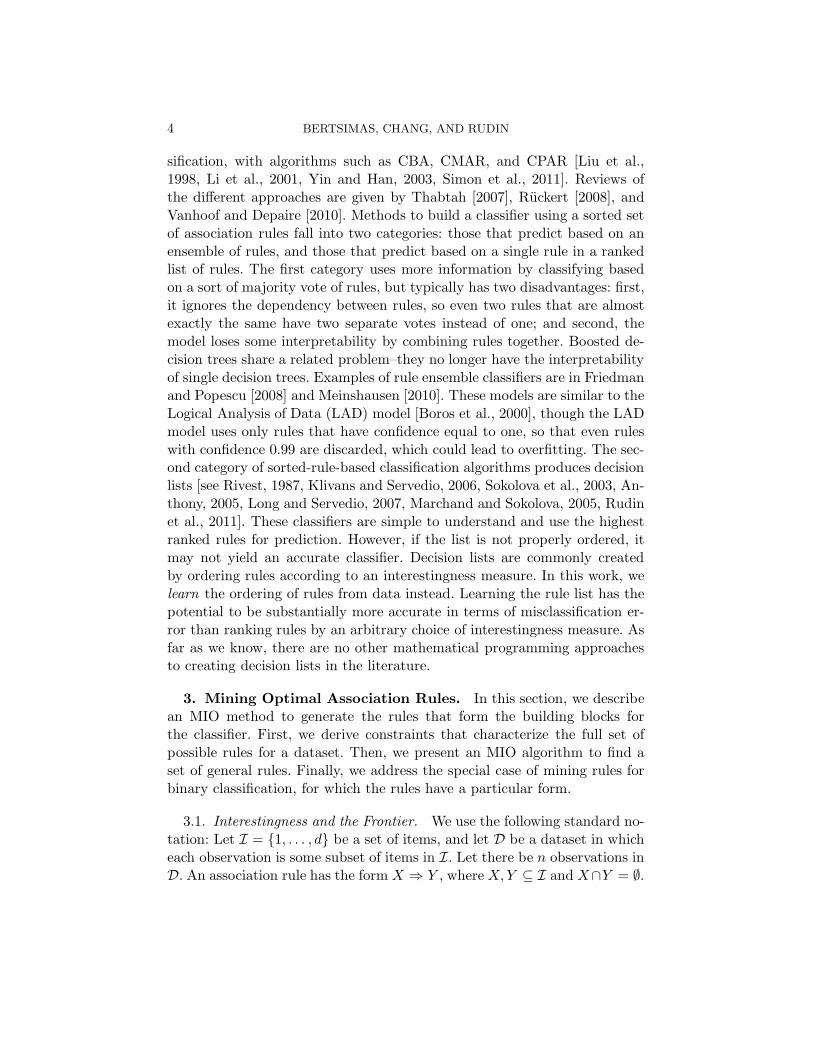
sification, with algorithms such as CBA, CMAR, and CPAR [Liu et al.,1998, Li et al., 2001, Yin and Han, 2003, Simon et al., 2011]. Reviews ofthe different approaches are given by Thabtah [2007], Ruckert [2008], andVanhoof and Depaire [2010]. Methods to build a classifier using a sorted setof association rules fall into two categories: those that predict based on anensemble of rules, and those that predict based on a single rule in a rankedlist of rules. The first category uses more information by classifying basedon a sort of majority vote of rules, but typically has two disadvantages: first,it ignores the dependency between rules, so even two rules that are almostexactly the same have two separate votes instead of one; and second, themodel loses some interpretability by combining rules together. Boosted de-cision trees share a related problem–they no longer have the interpretabilityof single decision trees. Examples of rule ensemble classifiers are in Friedmanand Popescu [2008] and Meinshausen [2010]. These models are similar to theLogical Analysis of Data (LAD) model [Boros et al., 2000], though the LADmodel uses only rules that have confidence equal to one, so that even ruleswith confidence 0.99 are discarded, which could lead to overfitting. The sec-ond category of sorted-rule-based classification algorithms produces decisionlists [see Rivest, 1987, Klivans and Servedio, 2006, Sokolova et al., 2003, An-thony, 2005, Long and Servedio, 2007, Marchand and Sokolova, 2005, Rudinet al., 2011]. These classifiers are simple to understand and use the highestranked rules for prediction. However, if the list is not properly ordered, itmay not yield an accurate classifier. Decision lists are commonly createdby ordering rules according to an interestingness measure. In this work, welearn the ordering of rules from data instead. Learning the rule list has thepotential to be substantially more accurate in terms of misclassification er-ror than ranking rules by an arbitrary choice of interestingness measure. Asfar as we know, there are no other mathematical programming approachesto creating decision lists in the literature.

3. Mining Optimal Association Rules. In this section, we describean MIO method to generate the rules that form the building blocks forthe classifier. First, we derive constraints that characterize the full set ofpossible rules for a dataset. Then, we present an MIO algorithm to find aset of general rules. Finally, we address the special case of mining rules forbinary classification, for which the rules have a particular form.

3.1. Interestingness and the Frontier. We use the following standard no-tation: Let I = {1, . . . , d} be a set of items, and let D be a dataset in whicheach observation is some subset of items in I. Let there be n observations inD. An association rule has the form X ⇒ Y , where X,Y ⊆ I and X∩Y = ∅.


We want to formulate a set of constraints that define the space P ofpossible rules. In what follows, the ti are data, while b, h, xi, yi, and zi arevariables. The binary vector ti ∈ {0, 1}d represents observation i:

tij = 1[observation i includes item j], 1 ≤ i ≤ n, 1 ≤ j ≤ d.

The binary vectors b, h ∈ {0, 1}d represent the body and head respectivelyof a given rule X ⇒ Y . That is, for j = 1, . . . , d,

bj = 1[j∈X] and hj = 1[j∈Y ].

We also use variables xi, yi, and zi, for i = 1, . . . , n, to represent

xi = 1[observation i includes X], yi = 1[observation i includes Y ], and

zi = 1[observation i includes X and Y ].

P is constrained by (1) through (10). Note that ed is the d-vector of ones.Each constraint is explained below.

bj + hj ≤ 1, ∀j,(1)

xi ≤ 1 + (tij − 1)bj , ∀i, j,(2)

xi ≥ 1 + (ti − ed)T b, ∀i,(3)

yi ≤ 1 + (tij − 1)hj , ∀i, j,(4)

yi ≥ 1 + (ti − ed)Th, ∀i,(5)

zi ≤ xi, ∀i,(6)

zi ≤ yi, ∀i,(7)

zi ≥ xi + yi − 1, ∀i,(8)

bj , hj ∈ {0, 1}, ∀j,(9)

0 ≤ xi, yi, zi ≤ 1, ∀i.(10)

Since an item cannot be in both the body and head of a rule (X ∩ Y = ∅),b and h must satisfy (1). To understand (2), consider the two cases bj = 0and bj = 1. If bj = 0, then the constraint is just xi ≤ 1, so the constrainthas no effect. If bj = 1, then the constraint is xi ≤ tij. That is, if bj = 1(item j is in X) but tij = 0 (item j is not in observation i), then xi = 0.This set of constraints implies that xi = 0 if observation i does not includeX. We need (3) to say that xi = 1 if observation i includes X. Note thattTi b is the number of items in the intersection of observation i and X, andeTd b is the number of items in X. Constraint (3) is valid because

tTi b =d∑

j=1

tijbj ≤d∑

j=1

bj = eTd b,


Table 1

The body X of the rule is in observation i since (2) and (3) are satisfied.

j1 2 3 4 5

ti (1 if item j in observation i, 0 otherwise) 1 0 1 1 0b (1 if item j in body of rule, 0 otherwise) 1 0 0 1 0

where equality holds if and only if observation i includes X and otherwisetTi b ≤ eTd b− 1. Table 1 helps to clarify (2) and (3). Constraints (4) and (5)capture the yi in the same way that (2) and (3) capture the xi. The zi are 1 ifand only if xi = yi = 1, which is captured by (6) through (8). Constraints (9)and (10) specify that b and h are restricted to be binary, while the values ofx, y, and z are restricted only to be between 0 and 1.

Each point in P corresponds to a rule X ⇒ Y , where X = {j : bj = 1}and Y = {j : hj = 1}. There are 2d binary variables and 3n continuousvariables. Computationally, it is favorable to reduce the number of integervariables, and here we explain why x, y, and z are not also restricted to beintegral. There are two cases when deciding whether X is in observation i.If it is, then (3) implies xi ≥ 1, so xi = 1. If it is not, then there exists jsuch that tij = 0 and bj = 1, so (2) implies xi ≤ 0, or xi = 0. Thus, in eithercase, xi is forced to be an integer, regardless of whether we specify it as aninteger variable. The argument is similar for yi. For zi, there are two caseswhen deciding whether X and Y are both in observation i. If they are, thenxi = yi = 1, so (8) implies zi ≥ 1, or zi = 1. If they are not, then either (6)or (7) implies zi ≤ 0, or zi = 0. Thus, zi is also always integral.

P grows exponentially in the number of items d = |I|. It includes the fullset of association rules, which is many more than we usually need or wish tocollect. In order to generate only the potentially interesting rules, we judgeeach rule according to three of its fundamental properties, namely

sX =1

n

n∑

i=1

xi, sY =1

n

n∑

i=1

yi, and s =1

n

n∑

i=1

zi,

called coverage, prevalence, and support respectively. When we refer to thesemeasures for a particular rule r, we use the notation sX(r), sY (r), and s(r);we omit the parenthetical “(r)” when referring to them in general. We nowdefine a partial order ≤p over the set of possible rules to rank them in orderof interestingness. Given two rules r and r∗, we have r ≤p r∗, or r∗ is atleast as interesting as r if and only if:

sX(r) ≥ sX(r∗), sY (r) ≥ sY (r∗), and s(r) ≤ s(r∗).


Moreover, r =p r∗ if and only if sX(r) = sX(r∗), sY (r) = sY (r∗), and

s(r) = s(r∗). In words, “r ≤p r∗” means the coverage and prevalence of r∗

are no greater than that of r, but the support of r∗ is at least that of r. LetF ∗ be the set of rules that are not dominated by any other rules, that is,

F∗ = {r : There does not exist any r such that r <p r.}.

The rules r ∈ F∗ fall along a three dimensional frontier in sX , sY , and s.For intuition on why this frontier reasonably captures interestingness,

consider the interestingness measure of confidence, which is the empiricalprobability of Y given X. Refer to the data in Tables 2 and 3. Suppose wehave 20 observations, and we wish to compare the interestingness of tworules: a {chips}⇒{guacamole} and b {cookies}⇒{milk}. In Case 1 in thetable, the two rules have equal coverage sX = 8

20 , but the support s is higherfor a ( 7

20 versus 520 ), so a has higher confidence (a is more interesting). In

Case 2, the rules have equal support s = 520 , but the coverage sX is lower

for b ( 820 versus 10

20), so b has higher confidence (b is more interesting).This example shows that higher support and lower coverage increase theconfidence of a rule; for other measures, lower prevalence also often increasesthe interestingness.

Table 2

Number of observations containing certainitems (assume 20 observations total in both

Case 1 and Case 2).

Case 1 Case 2

{chips} 8 10{cookies} 8 8

{chips, guacamole} 7 5{cookies, milk} 5 5

Table 3

Support, coverage, and confidenceof rules a {chips}⇒{guacamole}

and b {cookies}⇒{milk}.

Case 1 Case 2

supp 7/20 5/20a cov 8/20 10/20

conf 7/8 5/10supp 5/20 5/20

b cov 8/20 8/20conf 5/8 5/8

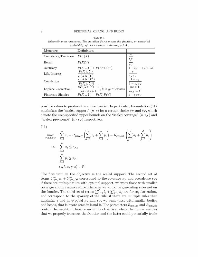
The point is that many measures in addition to confidence, includingthose in Table 4, increase with decreasing sX (holding sY and s constant),decreasing sY (holding sX and s constant), and increasing s (holding sXand sY constant). Thus, the rules that optimize each of these measures is inthe frontier F∗, and this is the set of rules that we focus on generating.

3.2. MIO Algorithm for General Association Rule Mining. We can findeach rule on the frontier F∗ corresponding to ≤p by putting upper boundson both sX and sY , and then maximizing s. We vary the bounds over all


Table 4

Interestingness measures. The notation P (A) means the fraction, or empiricalprobability, of observations containing set A.

Measure Definition

Confidence/Precision P (Y |X)s

sXRecall P (X |Y )

s

sYAccuracy P (X ∪ Y ) + P (Xc ∪ Y c) 1− sX − sY + 2s

Lift/InterestP (X ∪ Y )

P (X)P (Y )

s

sXsY

ConvictionP (X)P (Y c)

P (X ∪ Y c)

1− sY1− s/sX

Laplace CorrectionnP (X ∪ Y ) + 1

nP (X) + k, k is # of classes

ns+ 1

nsX + kPiatetsky-Shapiro P (X ∪ Y )− P (X)P (Y ) s− sXsY

possible values to produce the entire frontier. In particular, Formulation (11)maximizes the “scaled support” (n ·s) for a certain choice sX and sY , whichdenote the user-specified upper bounds on the “scaled coverage” (n ·sX) and“scaled prevalence” (n · sY ) respectively.

maxb,h,x,y,z

n∑

i=1

zi −Rgen xy

(

n∑

i=1

xi +n∑

i=1

yi

)

−Rgen bh

d∑

j=1

bj +d∑

j=1

hj

(11)

s.t.n∑

i=1

xi ≤ sX ,

n∑

i=1

yi ≤ sY ,

(b, h, x, y, z) ∈ P.

The first term in the objective is the scaled support. The second set ofterms

∑ni=1 xi +

∑ni=1 yi correspond to the coverage sX and prevalence sY ;

if there are multiple rules with optimal support, we want those with smallercoverage and prevalence since otherwise we would be generating rules not onthe frontier. The third set of terms

∑dj=1 bj +

∑dj=1 hj are for regularization,

and correspond to the sparsity of the rule; if there are multiple rules thatmaximize s and have equal sX and sY , we want those with smaller bodiesand heads, that is, more zeros in b and h. The parameters Rgen xy and Rgen bh

control the weight of these terms in the objective, where the former ensuresthat we properly trace out the frontier, and the latter could potentially trade


off sparsity for closeness to the frontier.Solving (11) once for each possible pair (sX , sY ) does not yield the entire

frontier since there may be multiple optimal rules at each point on thefrontier. To find other optima, we add constraints making each solutionfound so far infeasible, so that they cannot be found again when we re-solve.Specifically, for each pair (sX , sY ), we iteratively solve the formulation asfollows: Let (h∗, b∗) be the first optimum we find for (11). In each iteration,we add the constraint

(12)∑

j:b∗j=0

bj +∑

j:b∗j=1

(1− bj) +∑

j:h∗

j=0

hj +∑

j:h∗

j=1

(1− hj) ≥ 1

to the formulation. This constraint says that in either the vector b or thevector h, at least one of the components must be different from in the pre-vious solution; that is, at least one of the zeros must be one or one of theones must be zero. The previous solution bj = b∗j and hj = h∗j is infeasiblesince it would yield 0 ≥ 1 in (12). After adding this constraint, we solveagain. If the optimal value of s =

∑ni=1 zi decreases, then we exit the loop.

Otherwise, we have a new optimum, so we repeat the step above to generateanother constraint and re-solve.

3.3. MIO Algorithm for Associative Classification. As our main goal isto use association rules to construct a decision list for binary classification,we show in this section how to use MIO to mine rules for this purpose. Inthis case, the rules are of a specific form, either X ⇒ 1 or X ⇒ −1. That is,we prespecify the heads Y of the rules to be a class attribute, 1 or −1. Ourrule generation algorithm mines two separate frontiers of rules, one frontierfor each class.

Suppose we want rules on the frontier for a fixed class y ∈ {−1, 1}. LetS = {i : observation i has class label y}. Then s = 1

n

∑

i∈S xi. Since sY =|S| is equal for all rules of interest, we simplify the partial order (2) so thatgiven two rules r and r∗, we have r ≤p r

∗ if and only if:

sX(r) ≥ sX(r∗) and s(r) ≤ s(r∗).

Also, r =p r∗ if and only if sX(r) = sX(r∗) and s(r) = s(r∗). Each ruleon the corresponding two dimensional frontier in sX and s can be found byupper bounding sX and maximizing s. Since Y is fixed, we do not need theh, y, or z variables from (11). Formulation (13) finds a rule with maximum s


for a given upper bound sX on n · sX .

maxb,x

∑

i∈S

xi −Rgen x

n∑

i=1

xi −Rgen b

d∑

j=1

bj(13)

s.t.n∑

i=1

xi ≤ sX ,

xi ≤ 1 + (tij − 1)bj , ∀i, j,

xi ≥ 1 + (ti − ed)T b, ∀i,

bj ∈ {0, 1}, ∀j,

0 ≤ xi ≤ 1, ∀i.

The first term in the objective corresponds to support, and the otherscorrespond to coverage and sparsity, similar to the terms in (11). Solving (13)once for each value of sX does not yield the entire frontier since there maybe multiple optima. Analogous to the general case, we solve the formulationiteratively: Start by setting sX = n since the largest possible value of thescaled coverage is n. Let b∗ be the first optimum. Add the “infeasibilityconstraint”

(14)∑

j:b∗j=0

bj +∑

j:b∗j=1

(1− bj) ≥ 1

to the formulation, and solve again. If we find another optimum, then werepeat the step above to generate another constraint and re-solve. If theoptimal value of s =

∑

i∈S xi decreases, then we set the upper bound on sXto a smaller value and iterate again. Note that we can set this new value tobe the minimum of

∑ni=1 xi and sX−1 (previous bound minus one); we know

that no rule on the remainder of the frontier has scaled coverage greater than∑n

i=1 xi, so using this as the bound provides a tighter constraint than usingsX − 1 whenever

∑ni=1 xi < sX − 1.

Thus our rule generation algorithm, called “RuleGen,” generates the fron-tier, one rule at a time, from largest to smallest coverage. The details areshown in Figure 1. RuleGen allows optional minimum coverage thresholdsmincov−1 and mincov1 to be imposed on each of the classes of rules. Also,iter lim limits the number of times we iterate the procedure above for afixed value of sX with adding (14) between iterates. To find all rules on thefrontiers, set mincov−1 = mincov1 = 0 and iter lim = ∞.

To illustrate the steps of the algorithm, Figure 2 shows the followingfictitious example:


Set mincov−1, mincov1, iter lim.

For Y in {-1,1}

Initialize sX ← n, iter ← 1, s ← 0.

Initialize collection of rule bodies RY = ∅.

Repeat

If iter = 1 then

Solve (13) to obtain rule X⇒ Y.

s←∑

i∈S

x[i]

iter← iter+ 1

RY ←RY ∪ X

Add new constraint (14).

If iter ≤ iter lim then

Solve (13) to obtain rule X⇒ Y.

If∑

i∈S

x[i] < s then

sX← min

(

n∑

i=1

x[i], sX− 1

)

iter← 1

Else iter← iter+ 1

Else

sX← sX− 1

iter← 1

While sX ≥ n · mincovY

Fig 1. RuleGen algorithm. (Note sX=sX and s=s.)

a. Suppose we are constructing the frontier for data with n = 100. Initial-ize sX to n and solve (13). Assume the first solution has

∑

i∈S xi = 67.Then the algorithm adds the first rule to RY and sets s to 67. It addsthe infeasibility constraint (14) to (13) and re-solves. Assume the newrule still has

∑

i∈S xi = 67, so the algorithm adds this rule to RY, thenadds another infeasibility constraint to (13) and re-solves.

b. Assume the new rule has∑

i∈S xi = 65 and∑n

i=1 xi = 83 (correspond-ing to the support and coverage respectively). Since

∑

i∈S xi decreased,the algorithm sets sX to min (

∑ni=1 xi, sX− 1) = min(83, 99) = 83 be-

fore re-solving to obtain the next rule and adding it to RY.c. This process continues until the minimum coverage threshold is reached.


Fig 2. Illustrative example to demonstrate the steps in the RuleGen algorithm.

4. Building a Classifier. Suppose we have generated L rules, whereeach rule ℓ is of the form Xℓ ⇒ −1 or Xℓ ⇒ 1. Our task is now to rankthem to build a decision list for classification. Given a new observation, thedecision list classifies it according to the highest ranked rule ℓ such that Xℓ

is in the observation, or the highest rule that “applies.” In this section, wederive an empirical risk minimization algorithm using MIO that yields anoptimal ranking of rules. That is, the ordering returned by our algorithmmaximizes the (regularized) classification accuracy on a training sample.

We always include in the set of rules to be ranked two “null rules:”∅ ⇒ −1, which predicts class −1 for any observation, and ∅ ⇒ 1, whichpredicts class 1 for any observation. In the final ranking, the higher of thenull rules corresponds effectively to the bottom of the ranked list of rules;all observations that reach this rule are classified by it, thus the class itpredicts is the default class. We include both null rules in the set of rulesbecause we do not know which of them would serve as the better default,that is, which would help the decision list to achieve the highest possibleclassification accuracy; our algorithm learns which null rule to rank higher.

We use the following parameters:

piℓ =

1 if rule ℓ applies to observation i and predicts its class correctly,

−1 if rule ℓ applies to observation i but predicts its class incorrectly,

0 if rule ℓ does not apply to observation i,

viℓ = 1[rule ℓ applies to observation i] = |piℓ|,

Rrank = regularization parameter, trades off accuracy with conciseness,

and decision variables:

rℓ = rank of rule ℓ,

r∗ = rank of higher null rule,

uiℓ = 1[rule ℓ is the rule that predicts the class of observation i].


The rℓ variables store the ranks of the rules; r∗ is the rank of the defaultrule, which we want to be high for conciseness. The uiℓ variables help capturethe mechanism of the decision list, enforcing that only the highest applicablerule predicts the class of an observation: for observation i, uiℓ = 0 for allexcept one rule, which is the one, among those that apply, with the highestrank rℓ. The formulation to build the optimal classifier is:

maxr,r∗,g,u,s,α,β

n∑

i=1

L∑

ℓ=1

piℓuiℓ +Rrankr∗(15)

s.t.L∑

ℓ=1

uiℓ = 1, ∀i,(16)

gi ≥ viℓrℓ, ∀i, ℓ,(17)

gi ≤ viℓrℓ + L(1− uiℓ), ∀i, ℓ,(18)

uiℓ ≥ 1− gi + viℓrℓ, ∀i, ℓ,(19)

uiℓ ≤ viℓ, ∀i, ℓ,(20)

rℓ =L∑

k=1

ksℓk, ∀ℓ,(21)

L∑

k=1

sℓk = 1, ∀ℓ,(22)

L∑

ℓ=1

sℓk = 1, ∀k,(23)

r∗ ≥ rA,(24)

r∗ ≥ rB ,(25)

r∗ − rA ≤ (L− 1)α,(26)

rA − r∗ ≤ (L− 1)α,(27)

r∗ − rB ≤ (L− 1)β,(28)

rB − r∗ ≤ (L− 1)β,(29)

α+ β = 1,(30)

uiℓ ≤ 1−r∗ − rℓL− 1

, ∀i, ℓ,(31)

α, uiℓ, sℓk ∈ {0, 1}, ∀i, ℓ, k,

0 ≤ β ≤ 1,

rℓ ∈ {1, 2, . . . , L}, ∀ℓ.


Table 5

Observation ti is represented by {1 0 1 1 0}, and its class is −1. The highest rule thatapplies is the one ranked 8th (rℓ = 8) since {1 0 1 0 0}⊂{1 0 1 1 0} (the rules ranked10th and 9th do not apply). Thus uiℓ = 1 for this rule. This rule has piℓ = 1 since therule applies to ti and correctly predicts −1, so the contribution of observation i to the

accuracy part of the objective in (15) is∑L

ℓ=1piℓuiℓ = 1.

Observation ti: {1 0 1 1 0}, class=−1Ranked rules piℓ rℓ uiℓ

{0 1 0 0 1} ⇒ −1 0 10 0{0 1 1 0 0} ⇒ 1 0 9 0{1 0 1 0 0} ⇒ −1 1 8 1{1 0 0 0 1} ⇒ −1 0 7 0{0 0 0 0 0} ⇒ 1 1 6 0

......

......

{0 0 1 1 0} ⇒ −1 −1 1 0

The first term in the objective corresponds to classification accuracy.Given an ordering of rules, the quantity ci =

∑Lℓ=1 piℓuiℓ equals 1 if the

resulting decision list correctly predicts the class of observation i and −1otherwise. Thus, the number of correct classifications is

n∑

i=1

(

ci + 1

2

)

=1

2

(

n+n∑

i=1

ci

)

.

So to maximize classification accuracy, it suffices to maximize

n∑

i=1

ci =n∑

i=1

L∑

ℓ=1

piℓuiℓ.

Table 5 shows an example of the parameters (piℓ) and variables (rℓ, uiℓ) fora particular ranking of rules and observation to be classified.

Constraint (16) enforces that for each i, only one of the uiℓ variablesequals one while the rest are zero. To capture the definition of the uiℓ, wealso use auxiliary variables gi, which represent the highest rank of the rulessuch that Xℓ is in observation i. Through (17) and (18), there is only one ℓsuch that uiℓ = 1 is feasible, namely the ℓ corresponding to the highest valueof viℓrℓ. Constraints (19) and (20) help improve the linear relaxation andthus are intended to speed up computation. We assign the integral ranks rℓusing (21) through (23), which imply sℓk = 1 if rule ℓ is assigned to rank k.The matching between ranks and rules is one-to-one.

We add regularization in order to favor a shorter overall list of rules.That is, our regularizer pulls the rank of one of the null rules as high as


possible. If rA is the rank of ∅ ⇒ −1 and rB is the rank of ∅ ⇒ 1, then weadd r∗ to the objective function, where r∗ is the maximum of rA and rB .The regularization coefficient of r∗ in the objective is Rrank. We capture r∗using (24) through (30): Either α = 1 and β = 0 or β = 1 and α = 0. Ifα = 1, then r∗ = rB . If β = 1, then r∗ = rA. Since we are maximizing, r∗equals the higher of rA and rB . Note that if α is binary, then β need not bebinary because the constraint α + β = 1 forces integral values for β. If therank rℓ of rule ℓ is below r∗, then uiℓ = 0 for all i, so (31) is also valid, andwe include it to help speed up computation.

The Ordered Rules for Classification (ORC) algorithm consists of gener-ating rules using the method shown in Figure 1, computing the piℓ and viℓ,and then solving (15). The rule generation step could also be replaced by adifferent method, such as Apriori [Agrawal and Srikant, 1994]. We use ourinteger optimization approach in the experiments. Note that (13) and (15)are not restricted to binary classification problems; both formulations canbe directly applied in the multi-class setting.

5. Computational Results. We used a number of publicly availabledatasets to demonstrate the performance of our approach. Eight are fromthe UCI Machine Learning Repository: Breast Cancer Wisconsin (Origi-nal), Car Evaluation, Haberman’s Survival, Mammographic Mass, MONK’sProblem 2, SPECT Heart, Tic-Tac-Toe, and Congressional Voting Records[Asuncion and Newman, 2007]. Crime1 and Crime2 are derived from a studyfunded by the US Department of Justice [Courtney and Cusick, 2010]. Ti-tanic is from a report on the sinking of the “Titanic” [British Board of Trade,1990]. For each dataset, we divided the data evenly into three folds and usedeach fold in turn as a test set, training each time with the other two folds.The training and test accuracy were averaged over these three folds. Wecompared the ORC algorithm with six other classification methods—logisticregression [see Hastie et al., 2001, Dreiseitl and Ohno-Machado, 2002], Sup-port Vector Machines (SVM) [Vapnik, 1995, Burges, 1998], Classificationand Regression Trees (CART) [Breiman et al., 1984], C4.5 [Quinlan, 1993](J48 implementation), Random Forests [Breiman, 2001], and AdaBoost [Fre-und and Schapire, 1995]—all run using R 2.15.0. We used the radial basiskernel and regularization parameter C = 1 for SVM, and decision trees asbase classifiers for AdaBoost. The ORC algorithm was implemented usingILOG AMPL 11.210 with the Gurobi solver.1

1For B.Cancer, Mammo, MONK2, and TicTacToe, we used Gurobi 3.0.0 on a computerwith two Intel quad core Xeon E5440 2.83GHz processors and 32GB of RAM. For the otherdatasets, we used Gurobi 4.5.2 on a computer with an Intel quad core Xeon E5687 3.60GHzprocessor and 48GB of RAM.


Here we explain how we chose the parameter settings for the ORC exper-iments; these parameters were the same for all datasets. In generating ruleswith (13), we wanted to ensure that Rgen x was small enough that the solverwould never choose to decrease the scaled support

∑

i∈S xi just to decreasethe scaled coverage

∑ni=1 xi. That is, Rgen x should be such that we would

not sacrifice maximizing s for lower sX ; this required only that this param-eter be a small positive constant, so we chose Rgen x = 0.1

n. Similarly, we

did not want to sacrifice maximizing s or lowering sX for greater sparsity,so we chose Rgen b = 0.1

nd. In order to not sacrifice classification accuracy for

a shorter decision list in ranking the rules with (15), we chose Rrank = 1L.

We also used a minimum coverage threshold of 0.05, and iterated up to fivetimes at each setting of sX (mincov−1 = mincov1 = 0.05, iter lim = 5);these choices were based on preliminary experiments to determine parame-ters that would yield a reasonable number of rules.

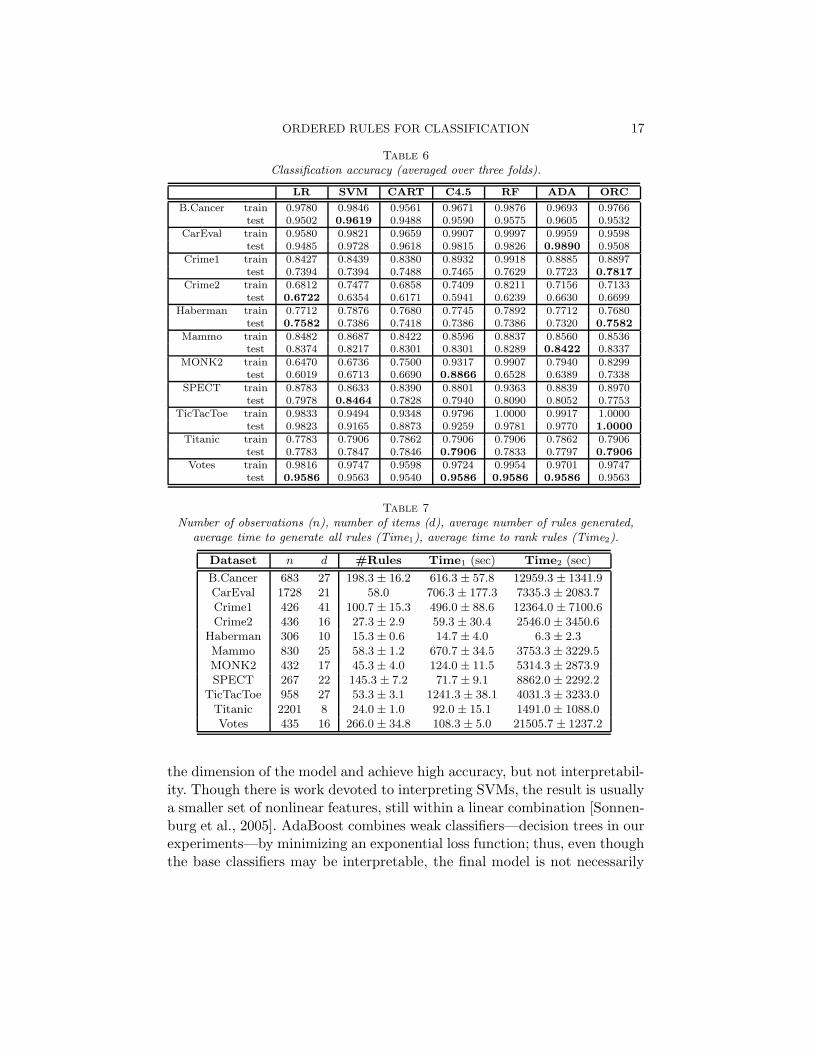
Table 6 shows the average training and test classification accuracy foreach dataset; corresponding standard deviations are in the appendix. Boldindicates the highest average in the row. Table 7 shows the dataset sizes aswell as average number of rules generated by RuleGen and average runtimesfor our algorithms (±one standard deviation); runtimes for the other meth-ods were too small to be a significant factor in assessment. Time1 is the totaltime for generating all rules; Time2 is the time when the final solution wasfound, either before solving to optimality or before being terminated after aspecified time limit. We generally terminated the solver before (15) solvedto provable optimality. The appendix includes more detail about the exper-iments. Table 8 shows a pairwise comparison of the ORC algorithm to theother algorithms; for each of the other methods, the table contains a countof the number of datasets for which the method is more accurate, equallyaccurate, or less accurate than ORC. These results show that in terms ofaccuracy, the ORC algorithm is on par with top classification methods.

6. Interpretability. Interpretability is subjective, but in this section,we aim to demonstrate that the ORC classifier performs well in terms ofbeing easy to understand. Classifiers generated by CART and C4.5 are in-terpretable because of their decision tree structure. Other methods are notas easily interpreted. For example, the logistic regression model is

p =1

1 + e−β0+βT t,

where p is the probability that the class of observation t is 1. The SVMmodel is a hyperplane that maximizes the margin between the hyperplaneand the closest point to it from both classes; by using kernels, we can raise


Table 6

Classification accuracy (averaged over three folds).

LR SVM CART C4.5 RF ADA ORC

B.Cancer train 0.9780 0.9846 0.9561 0.9671 0.9876 0.9693 0.9766test 0.9502 0.9619 0.9488 0.9590 0.9575 0.9605 0.9532

CarEval train 0.9580 0.9821 0.9659 0.9907 0.9997 0.9959 0.9598test 0.9485 0.9728 0.9618 0.9815 0.9826 0.9890 0.9508

Crime1 train 0.8427 0.8439 0.8380 0.8932 0.9918 0.8885 0.8897test 0.7394 0.7394 0.7488 0.7465 0.7629 0.7723 0.7817

Crime2 train 0.6812 0.7477 0.6858 0.7409 0.8211 0.7156 0.7133test 0.6722 0.6354 0.6171 0.5941 0.6239 0.6630 0.6699

Haberman train 0.7712 0.7876 0.7680 0.7745 0.7892 0.7712 0.7680test 0.7582 0.7386 0.7418 0.7386 0.7386 0.7320 0.7582

Mammo train 0.8482 0.8687 0.8422 0.8596 0.8837 0.8560 0.8536test 0.8374 0.8217 0.8301 0.8301 0.8289 0.8422 0.8337

MONK2 train 0.6470 0.6736 0.7500 0.9317 0.9907 0.7940 0.8299test 0.6019 0.6713 0.6690 0.8866 0.6528 0.6389 0.7338

SPECT train 0.8783 0.8633 0.8390 0.8801 0.9363 0.8839 0.8970test 0.7978 0.8464 0.7828 0.7940 0.8090 0.8052 0.7753

TicTacToe train 0.9833 0.9494 0.9348 0.9796 1.0000 0.9917 1.0000test 0.9823 0.9165 0.8873 0.9259 0.9781 0.9770 1.0000

Titanic train 0.7783 0.7906 0.7862 0.7906 0.7906 0.7862 0.7906test 0.7783 0.7847 0.7846 0.7906 0.7833 0.7797 0.7906

Votes train 0.9816 0.9747 0.9598 0.9724 0.9954 0.9701 0.9747test 0.9586 0.9563 0.9540 0.9586 0.9586 0.9586 0.9563

Table 7

Number of observations (n), number of items (d), average number of rules generated,average time to generate all rules (Time1), average time to rank rules (Time2).

Dataset n d #Rules Time1 (sec) Time2 (sec)

B.Cancer 683 27 198.3 ± 16.2 616.3 ± 57.8 12959.3 ± 1341.9CarEval 1728 21 58.0 706.3 ± 177.3 7335.3 ± 2083.7Crime1 426 41 100.7 ± 15.3 496.0 ± 88.6 12364.0 ± 7100.6Crime2 436 16 27.3± 2.9 59.3 ± 30.4 2546.0 ± 3450.6

Haberman 306 10 15.3± 0.6 14.7± 4.0 6.3± 2.3Mammo 830 25 58.3± 1.2 670.7 ± 34.5 3753.3 ± 3229.5MONK2 432 17 45.3± 4.0 124.0 ± 11.5 5314.3 ± 2873.9SPECT 267 22 145.3 ± 7.2 71.7± 9.1 8862.0 ± 2292.2

TicTacToe 958 27 53.3± 3.1 1241.3 ± 38.1 4031.3 ± 3233.0Titanic 2201 8 24.0± 1.0 92.0 ± 15.1 1491.0 ± 1088.0Votes 435 16 266.0 ± 34.8 108.3 ± 5.0 21505.7 ± 1237.2

the dimension of the model and achieve high accuracy, but not interpretabil-ity. Though there is work devoted to interpreting SVMs, the result is usuallya smaller set of nonlinear features, still within a linear combination [Sonnen-burg et al., 2005]. AdaBoost combines weak classifiers—decision trees in ourexperiments—by minimizing an exponential loss function; thus, even thoughthe base classifiers may be interpretable, the final model is not necessarily


Table 8

Number of datasets for which each algorithm exceeded, tied, or fell below ORC inclassification accuracy.

>ORC =ORC <ORC

LR 4 1 6SVM 3 1 7CART 2 0 9C45 5 1 5RF 4 0 7ADA 5 0 6

Table 9

Average number of leaves for CART and C4.5, average length of decision list for ORC.

CART C4.5 ORC

B.Cancer 5 5.3 12.7CarEval 14 27.7 12.7Crime1 11.3 16.3 21Crime2 8.3 16.3 9.3SPECT 6.3 7.7 18Haber 4.7 3.7 4.3Mammo 4 8.7 12.3MONK2 14.7 29.3 19.7TicTacToe 21 34.7 9Titanic 3.7 5 3.3Votes 3 4.7 7.3

Average 8.7 14.5 11.8Standard Deviation 5.8 11.3 5.9

as interpretable. Random Forests also combines trees.Recall that we want our models to be concise because simpler models

are easier to understand. Though we cannot exactly compare concisenessamong different types of models, one reasonable measure for decision treesand lists is the number of rules. Table 9 shows the number of rules in themodels generated by CART, C4.5, and ORC for each dataset, averaged overthe three folds. For CART and C4.5, the number of rules is the number ofleaves; for ORC, it is the number of rules above and including the default.In general, the ORC decision lists are larger models than those produced byCART, but can be significantly smaller than those produced by C4.5. Thestandard deviations in the bottom row of Table 9 also indicate that ORCproduces a more consistently small model compared to C4.5.

In the remainder of this section, we show the decision lists for a few of thedatasets from Section 5 as examples of the interpretability of the decisionlists produced by ORC.


Table 10

Rules for predicting whether a patient survived at least five years (+5) or not (<5).

s sX Rule

1 80 93 Number of nodes = 0 ⇒ 5+2 53 83 1 ≤ Number of nodes ≤ 9 ⇒ 5+3 18 55 40 ≤ Age ≤ 49 ⇒ <54 20 71 50 ≤ Age ≤ 59 ⇒ <55 147 204 Default ⇒ 5+

6.1. Haberman’s Survival. In this dataset, each “observation” representsa patient who underwent surgery for breast cancer. The goal is to predictwhether the patient survived at least five years (5+) or not (< 5). Table 10shows the ORC classifier from training on Folds 1 and 2. We can easily statein words how this classifier makes predictions:

1. If the patient has no more than nine positive axillary nodes, then sheis classified as 5+.

2. If she has more than nine nodes and is in her 40s or 50s, then she isclassified as <5.

3. Otherwise, she is classified as 5+.

6.2. Crime. The Crime1 and Crime2 datasets were derived from a studyof crime among youth as they transition to adulthood. There were threewaves of interviews—the first when the youth were between 17 and 18 yearsof age, the second when they were between 19 and 20, and the third whenthey turned 21. Table 11 shows some of the binary variables from the firsttwo waves. Using the data, we can design a number of prediction problems.The two problems corresponding to Crime1 and Crime2 are:

• Crime1: Based on the 41 binary variables fromWaves 1 and 2, predictwhether or not a youth is arrested between the Wave 2 and Wave 3 in-terviews. There were 426 observations after removing those with miss-ing values.

• Crime2: Based on the 16 variables in the top half of Table 11 thatdescribe the background of the youth, predict whether a youth reportsa violent offense at any of the Wave 1, 2, or 3 interviews. There were432 observations after removing those with missing values.

As an example of the kind of interpretable result we can obtain from theCrime2 data, Table 12 shows the decision list from training on Folds 1 and 3.


Table 11

Variable descriptions.

Variable Description

Female Respondent is femaleMale Respondent is male

Hispanic Respondent is hispanicWhite Respondent is whiteBlack Respondent is black

OtherRace Respondent is mixed or other raceAlcoholOrSubstanceAbuse Alcohol or substance abuse diagnosisMentalHealthDiagnosis Mental health diagnosis

TeenageParent Respondent is a teenage parentSexAbuseVictim Victim of sex abuseInFosterCare W1 In foster care at Wave 1InKinshipCare W1 In kinship care at Wave 1InGroupCare W1 In group care at Wave 1

IndependentOtherCare W1 Independent living or other care at Wave 1NoMomOrStepmom No mom or stepmomNoDadOrStepdad No dad or stepdad

PropertyDamage W1 Deliberately damaged property at Wave 1StoleOver50 W1 Stole something worth >$50 at Wave 1

SoldMarijuanaOrDrugs W1 Sold marijuana or other drugs at Wave 1BadlyInjuredSomeone W1 Badly injured someone at Wave 1

UsedWeapon W1 Used or threatened to use a weapon at Wave 1ViolentOffense W1 Violent offense at Wave 1

NonviolentOffense W1 Nonviolent offense at Wave 1ViolentOffense W2 Violent offense at Wave 2

NonviolentOffense W2 Nonviolent offense at Wave 2ArrestedBetweenW1andW2 Arrested since Wave 1 at Wave 2

InSchool W1 In school at Wave 1Employed W1 Employed at Wave 1InSchool W2 In school at Wave 2Employed W2 Employed at Wave 2

Table 12

Rules for predicting whether there is a violent offense in any wave (1) or not (−1).

s sX Rule

1 29 41 InGroupCare W1 ⇒ 12 13 19 Female, SexAbuseVictim, IndependentOtherCare W1 ⇒ −13 13 16 AlcoholOrSubstanceAbuse, MentalHealthDiagnosis ⇒ 14 14 26 Female, Black, InFosterCare W1 ⇒ −15 103 154 Black ⇒ 16 32 53 Female, White ⇒ −17 41 58 AlcoholOrSubstanceAbuse ⇒ 18 119 291 Default ⇒ −1


6.3. Titanic. Each row of this dataset represents one of the 2201 passen-gers aboard the Titanic, a passenger liner that sank in 1912 after strikingan iceberg. The features of the dataset are: social class (first, second, third,crew), age (adult, child), and gender (male or female). We want to predictwhether or not each passenger survived. Table 13 shows the decision list fromtraining on Folds 2 and 3. This result makes sense in light of the “womenand children first” policy and the fact that little effort was made to help thethird-class passengers.

Table 13

Rules for predicting whether a passenger survived the Titanic sinking (1) or not (−1).

s sX Rule

1 341 462 Third Class ⇒ −12 888 1108 Adult, Male ⇒ −13 477 1467 Default ⇒ 1

6.4. Tic-Tac-Toe. Our final example is the Tic-Tac-Toe dataset. Eachdata point represents a board configuration at the end of a Tic-Tac-Toegame where player x played first, and the classification problem is to identifywhether player x won. This is an easy task for a human, who needs onlyto determine if there are three x’s in a row. There are nine features inthe original data, each representing a square on a Tic-Tac-Toe board. Thepossible values for each feature are: x, o, or b (player x, player o, or blank).

This example demonstrates that for certain datasets, the ORC algorithmmay have a substantial advantage by optimizing both accuracy and concise-ness. Figure 3 shows the CART classifier from training on Folds 1 and 2.The notation o.5 means ‘o’ in box 5, x.7 means ‘x’ in box 7, etc. Figure 4shows the C4.5 classifier. The ORC classifier, shown in Figure 5, decidesthe class of a board the same way a typical human would: if the board hasthree x’s in a row, which can occur in eight different configurations, thenplayer x wins; otherwise, player x does not win. It achieves perfect accuracyin training and testing; the accuracies of CART and C4.5 are about 0.94and 0.99 respectively for training and 0.88 and 0.93 respectively for testing.The ORC classifier is much more concise than either of those produced byCART or C4.5. It has only nine rules, versus 21 for CART and 36 for C4.5.

7. Large-Scale Models. MIO is computationally intensive, as illus-trated in Table 7. Nevertheless, even for large datasets, our MIO approachhas the potential to order rules into an accurate decision list. The runtimesin the Time2 column of Table 7 could in fact be substantially shorter if we


Fig 3. CART Classifier for Tic-Tac-Toe dataset (predicted class in parentheses).

Fig 4. C4.5 Classifier for Tic-Tac-Toe dataset (predicted class in parentheses), left branchalways means ‘no’ and right branch always means ‘yes.’


1

win x

s=54 x

sX=54 x

2

win x

s=61 x

sX=61 x

3

win x x x

s=42

sX=42

4

win

s=54

sX=54 x x x

5

win x

s=57 x

sX=57 x

6

win x

s=61 x

sX=61 x

7

win x

s=54 x

sX=54 x

8

win

s=55 x x x

sX=55

9

no win

s=215

sX=638

Fig 5. Rules for predicting whether player x wins a Tic-Tac-Toe game.

were seeking just a good solution rather than an optimal solution. The MIOsolver typically finds a good solution quickly, but takes longer to improveupon it and to finally prove optimality. As it was not our goal to obtain asolution in the shortest time possible, we allowed the solver to search for thebest solution it could find in a reasonable amount of time. For larger datasetsthan those shown in Section 5, we can run (15) just until we obtain a goodsolution, or let it run for a longer period of time to obtain better solutions.As the speed of computers continues to advance exponentially, and also ascloud computing becomes more accessible, we expect our MIO approach toproduce high quality solutions with decreasing computing effort.

In this section, we show results on an additional dataset from the UCIRepository, Wine Quality, which has n = 4898 observations and d = 44items, yielding a data table with nd = 215, 512 entries. The largest datasetin Section 5 was CarEval, which had nd = 36, 288. The large size of theWine dataset caused long runtimes for (13), which we did want to solve tooptimality to obtain rules on the frontier. Thus we used Apriori to generatethe rules instead. We ran Apriori using R, and specified minimum supportthresholds of 0.006 and 0.1 for the positive and negative class rules respec-tively to generate a reasonable number of rules. Otherwise, our experimentalsetup was the same as for the other datasets; we divided the data into threefolds, and to rank the rules, we used (15) with Rrank = 1

L. We let (15) run

for approximately 20 hours. Figure 6 shows the accuracy of the solutionsfound by the solver over time. (Train12 refers to training on Folds 1 and 2,Train13 refers to training on Folds 1 and 3, and Train23 refers to trainingon Folds 2 and 3.) The figure illustrates how a good solution is often foundrelatively quickly but then improves only slowly. Averaged over three folds,we generated 71.3 rules, and the time to find the final solution of (15) be-fore termination was 57258.3 seconds. Table 14 shows the accuracy of the


algorithms. ORC achieves about the same accuracy as SVM and AdaBoost,though Random Forests achieved the highest accuracy for this dataset.

In terms of interpretability, ORC produces a much more concise modelthan C4.5. Averaged over three folds, the C4.5 trees have 184.7 leaves,whereas the ORC lists have 25.3 rules in addition to higher test accuracythan C4.5. (CART was even more concise, with an average of 4.7 leaves,but it lost accuracy.) This is another example of the consistency of the ORCalgorithm in producing classification models that have interpretability ad-vantages and compete well against the best methods in accuracy.

0 5 10 15 20

0.0

0.2

0.4

0.6

0.8

1.0

Accuracy Along Solution Paths

Time (hours)

Cla

ssifi

catio

n A

ccur

acy

Train12Train13Train23

Fig 6. Accuracy of solutions found by ORC algorithm over time for Wine data.

Table 14

Classification accuracy for Wine dataset (averaged over three folds).


Wine train 0.8040 0.8460 0.7850 0.9129 0.9918 0.8432 0.8304test 0.7987 0.8105 0.7842 0.8085 0.8608 0.8105 0.8103

8. Conclusion. In this work, we developed algorithms for producinginterpretable, yet accurate, classifiers. The classifiers we build are decisionlists, which use association rules as building blocks. Both of the challengesaddressed in this work, namely the task of mining interesting rules, and thetask of ordering them, have always been hampered by “combinatorial ex-plosion.” Even with a modest number of items in the dataset, there may


be an enormous number of possible rules, and even with a modest num-ber of rules, there are an enormous number of ways to order them. On theother hand, MIO methods are naturally suited to handle such problems;they not only encode the combinatorial structure of rule mining and ruleordering problems, but also are able to capture the new forms of regular-ization introduced in this work, that is, favoring more compact rules andshorter lists. Our computational experiments show that ORC competes wellin terms of accuracy against the top classification algorithms on a variety ofdatasets. In our paper, we used only one setting of the parameters for all ofthe experiments to show that even an “untuned” version of our algorithmperforms well; however, by varying these parameters, it may be possible toachieve still better predictive performance. Since our paper is among thefirst to use MIO methods for machine learning, and in particular to createdecision lists using optimization-based (non-heuristic) approaches, it opensthe door for further research on how to use optimization-based approachesfor rule mining, creating interpretable classifiers, and handling new forms ofregularization.

APPENDIX A: DETAILS FROM COMPUTATIONAL EXPERIMENTS

As explained in Section 3, each observation in our data is representedby a binary vector. Six of the datasets used in our experiments had onlycategorical variables: CarEval, MONK2, SPECT, TicTacToe, Titanic, andVotes. Thus it was straightforward to transform them into binary features.Here we describe how we transformed the other datasets:

1. Breast Cancer Wisconsin (Original). The dataset has 699 rows.There are 683 remaining observations after removing rows with missingvalues. There are nine original features, each taking integer valuesbetween 1 and 10. We used categorical variables to capture whethereach feature is between 1 and 4, 5 and 7, or 8 and 10.

2. Crime1 and Crime2. The derivation of these datasets is describedin Section 6.

3. Haberman’s Survival. The dataset has three features: age, year ofoperation, and number of positive axillary nodes. We removed thesecond feature since it did not seem to be predictive of survival andthus would not contribute to interpretability. We split the age featureinto five bins by decades: 39 and under, 40 to 49, 50 to 59, 60 to 69,and 70 and over. We also split the nodes feature into five bins: none,1 to 9, 10 to 19, 20 to 29, and at least 30.

4. Mammographic Mass. The dataset has 961 rows, each representinga patient. There are 830 remaining observations after removing rows


with missing values. The only feature that is not categorical is patientage, which we split into seven bins: 29 and under, 30 to 39, 40 to 49,50 to 59, 60 to 69, 70 to 79, and 80 and over.

5. Wine Quality. We used the data for white wine. All features werecontinuous, so we binned them by quartiles. A wine was in class 1 ifits quality score between 7 and 10, and class −1 if its quality scorewas between 1 and 6.

Table 15 shows the standard deviations that correspond to the averages inTable 6. Table 16 shows the following results for each dataset (Train12 refersto training on Folds 1 and 2, Train13 refers to training on Folds 1 and 3, andTrain23 refers to training on Folds 2 and 3): L−1 and L1 are the numbers ofrules generated by RuleGen for class −1 and class 1 respectively. Time1 isthe total time for generating all L−1+L1 rules; Time2 is the time when thefinal solution was found, either before solving to optimality or before beingterminated after a specified amount of time. Table 16 also shows the timelimit we used for each of the different datasets. For some datasets, the timelimit was significant longer than Time2, illustrating how it can take a longtime for the solver to reach provable optimality even though the solutionappears to have converged. Note that in running (15) for the TicTacToedataset, Train12 solved to optimality in 1271 seconds; Train12 and Train23had optimality gaps of about 0.02% and 0.01% respectively when the finalsolutions were found.

Table 17 shows the average classification accuracy for three methods, twoof which are SVM and ORC from Table 6. The other is a tuned version ofSVM, where we varied the C parameter and chose the one with the bestaverage test performance in hindsight. The overall performance of the un-tuned ORC algorithm is still on par with that of the tuned SVM algorithm.

REFERENCES

Rakesh Agrawal and Ramakrishnan Srikant. Fast algorithms for mining association rules.In Proceedings of the 20th International Conference on Very Large Databases, pages487–499, 1994.

Rakesh Agrawal, Tomasz Imielinski, and Arun Swami. Mining association rules betweensets of items in large databases. In Proceedings of the 1993 ACM SIGMOD InternationalConference on Management of Data, pages 207–216, 1993.

Martin Anthony. Decision lists. Technical report, CDAM Research Report LSE-CDAM-2005-23, 2005.

A. Asuncion and D.J. Newman. UCI machine learning repository, 2007. URLhttp://www.ics.uci.edu/ mlearn/MLRepository.html.

Roberto J. Bayardo and Rakesh Agrawal. Mining the most interesting rules. In Proceedings


Table 15

Standard deviation of classification accuracy.


B.Cancer train 0.0114 0.0022 0.0110 0.0137 0.0064 0.0116 0.0108test 0.0417 0.0142 0.0091 0.0167 0.0198 0.0274 0.0091

CarEval train 0.0027 0.0018 0.0035 0.0018 0.0005 0.0018 0.0093test 0.0027 0.0066 0.0046 0.0044 0.0076 0.0044 0.0036

Crime1 train 0.0108 0.0318 0.0070 0.0073 0.0020 0.0054 0.0073test 0.0244 0.0141 0.0147 0.0070 0.0267 0.0041 0.0186

Crime2 train 0.0217 0.0169 0.0484 0.0273 0.0066 0.0219 0.0258test 0.0559 0.0369 0.0366 0.0402 0.0376 0.0438 0.0700

Haberman train 0.0247 0.0221 0.0221 0.0321 0.0225 0.0172 0.0242test 0.0442 0.0204 0.0453 0.0484 0.0283 0.0204 0.0442

Mammo train 0.0136 0.0088 0.0076 0.0036 0.0020 0.0089 0.0165test 0.0249 0.0245 0.0217 0.0097 0.0115 0.0240 0.0202

MONK2 train 0.0256 0.0035 0.0284 0.0361 0.0053 0.0231 0.0217test 0.0526 0.0145 0.0729 0.0743 0.0208 0.0139 0.0356

SPECT train 0.0399 0.0366 0.0227 0.0117 0.0032 0.0141 0.0471test 0.0297 0.0619 0.0425 0.0507 0.0195 0.0234 0.0389

TicTac train 0.0080 0.0133 0.0047 0.0072 0.0000 0.0048 0.0000test 0.0148 0.0262 0.0061 0.0066 0.0156 0.0095 0.0000

Titanic train 0.0037 0.0054 0.0055 0.0054 0.0054 0.0087 0.0054test 0.0074 0.0143 0.0106 0.0108 0.0120 0.0101 0.0108

Votes train 0.0190 0.0020 0.0105 0.0103 0.0020 0.0121 0.0072test 0.0276 0.0080 0.0159 0.0138 0.0000 0.0000 0.0080

Wine train 0.0037 0.0019 0.0047 0.0107 0.0013 0.0009 0.0007test 0.0142 0.0050 0.0055 0.0029 0.0053 0.0120 0.0035

of the 5th ACM SIGKDD International Conference on Knowledge Discovery and DataMining, pages 145–154, 1999.

Endre Boros, Peter L. Hammer, Toshihide Ibaraki, Alexander Kogan, Eddy Mayoraz, andIlya Muchnik. An implementation of logical analysis of data. IEEE Transactions onKnowledge and Data Engineering, 12(2):292–306, 2000.

Leo Breiman. Random forests. Machine Learning, 45(1):5–32, 2001.Leo Breiman, Jerome H. Friedman, Richard A. Olshen, and Charles J. Stone. Classification

and Regression Trees. Wadsworth, 1984.British Board of Trade. Report on the loss of the ‘Titanic’ (s.s.). In British Board of

Trade Inquiry Report (reprint). Gloucester, UK: Allan Sutton Publishing, 1990.Oliver Buchter and Rudiger Wirth. Discovery of association rules over ordinal data: A

new and faster algorithm and its application to basket analysis. 1394:36–47, 1998.Christopher J.C. Burges. A tutorial on support vector machines for pattern recognition.

Data Mining and Knowledge Discovery, 2:121–167, 1998.Mark E. Courtney and Gretchen Ruth Cusick. Crime during the transition to adulthood:

How youth fare as they leave out-of-home care in Illinois, Iowa, and Wisconsin, 2002-2007. Technical report, Ann Arbor, MI: Inter-university Consortium for Political andSocial Research [distributor], 2010.

Stephan Dreiseitl and Lucila Ohno-Machado. Logistic regression and artificial neural net-work classification models: a methodology review. Journal of Biomedical Informatics,35:352–359, 2002.

Yoav Freund and Robert Schapire. A decision-theoretic generalization of on-line learningand an application to boosting. Computational Learning Theory, 904:23–37, 1995.


Table 16

Number of rules generated for the negative (L−1) and positive (L1) classes, average timein seconds to generate all rules (Time1), average time in seconds to rank rules (Time2),

time limit on ranking rules.

L−1 L1 Time1 Time2 Limit on Time2

Train12 123 66 551 12802B.Cancer Train13 136 53 637 11703 14400 (4 hours)

Train23 135 82 661 14373Train12 45 13 598 8241

CarEval Train13 45 13 610 4952 21600 (6 hours)Train23 48 10 911 8813Train12 60 58 582 15481

Crime1 Train13 70 25 501 17373 18000 (5 hours)Train23 43 46 405 4238Train12 17 12 94 6489

Crime2 Train13 15 14 47 1071 7200 (2 hours)Train23 13 11 37 78Train12 6 10 19 9

Haber Train13 4 11 11 5 600 (10 minutes)Train23 5 10 14 5Train12 33 26 637 1340

Mammo Train13 29 28 706 2498 10800 (3 hours)Train23 29 30 669 7422Train12 28 21 135 2786

MONK2 Train13 30 16 125 8440 10800 (3 hours)Train23 27 14 112 4717Train12 10 127 73 9611

SPECT Train13 6 144 62 10686 10800 (3 hours)Train23 10 139 80 6289Train12 11 43 1278 1232

TicTacToe Train13 14 36 1202 3292 10800 (3 hours)Train23 12 44 1244 7570Train12 13 10 75 295

Titanic Train13 15 10 104 1756 7200 (2 hours)Train23 15 9 97 2422Train12 110 116 103 22899

Votes Train13 137 146 109 20536 25200 (7 hours)Train23 141 148 113 21082Train12 34 41 – 58978

Wine Train13 35 34 – 39483 74000 (∼20 hours)Train23 35 35 – 73314

Jerome H. Friedman and Bogdan E. Popescu. Predictive learning via rule ensembles. TheAnnals of Applied Statistics, 2(3):916–954, 2008.

Liqiang Geng and Howard J. Hamilton. Interestingness measures for data mining: a survey.ACM Computing Surveys, 38, September 2006.

Bart Goethals. Survey on frequent pattern mining. Technical report, Helsinki Institutefor Information Technology, 2003.

Jiawei Han, Hong Cheng, Dong Xin, and Xifeng Yan. Frequent pattern mining: currentstatus and future directions. Data Mining and Knowledge Discovery, 15:55–86, 2007.

Trevor Hastie, Robert Tibshirani, and Jerome H. Friedman. The elements of statisticallearning: data mining, inference, and prediction. Springer, New York, 2001.

Jochen Hipp, Ulrich Guntzer, and Gholamreza Nakhaeizadeh. Algorithms for association


Table 17

Results of tuned SVM (highest in row highlighted in bold).

Dataset SVM (default C = 1) SVM (hindsight) C ORC

B.Cancer train 0.9846± 0.0022 0.9868 ± 0.0044 1.2 0.9766 ± 0.0108test 0.9619± 0.0142 0.9634± 0.0203 0.9532 ± 0.0091

CarEval train 0.9821± 0.0018 1 7.2 0.9598 ± 0.0093test 0.9728± 0.0066 0.9988± 0.0010 0.9508 ± 0.0036

Crime1 train 0.8439± 0.0318 0.9648 ± 0.0035 4.6 0.8897 ± 0.0073test 0.7394± 0.0141 0.7512 ± 0.0361 0.7817± 0.0186

Crime2 train 0.7477± 0.0169 0.6996 ± 0.0216 0.4 0.7133 ± 0.0258test 0.6354± 0.0369 0.6445 ± 0.0391 0.6699± 0.0700

Haberman train 0.7876± 0.0221 0.7761 ± 0.0279 0.4 0.7680 ± 0.0242test 0.7386± 0.0204 0.7582± 0.0442 0.7582± 0.0442

Mammo train 0.8687± 0.0088 0.8608 ± 0.0095 0.6 0.8536 ± 0.0165test 0.8217± 0.0245 0.8313 ± 0.0197 0.8337± 0.0202

MONK2 train 0.6736± 0.0035 0.6736 ± 0.0035 1 0.8299 ± 0.0217test 0.6713± 0.0145 0.6713 ± 0.0145 0.7338± 0.0356

SPECT train 0.8633± 0.0366 0.8745 ± 0.0319 1.2 0.8970 ± 0.0471test 0.8464± 0.0619 0.8502± 0.0566 0.7753 ± 0.0389

TicTacToe train 0.9494± 0.0133 0.9901 ± 0.0009 6 1test 0.9165± 0.0262 0.9844 ± 0.0143 1

Titanic train 0.7906± 0.0054 0.7906 ± 0.0054 1 0.7906 ± 0.0054test 0.7847± 0.0143 0.7847 ± 0.0143 0.7906± 0.0108

Votes train 0.9747± 0.0020 0.9793 ± 0.0034 1.4 0.9747 ± 0.0072test 0.9563± 0.0080 0.9586± 0.0069 0.9563 ± 0.0080

Wine train 0.8460± 0.0019 0.9117 ± 0.0079 4.8 0.8304 ± 0.0007test 0.8105± 0.0050 0.8348± 0.0035 0.8103 ± 0.0035

rule mining - a general survey and comparison. SIGKDD Explorations, 2:58–64, June2000.

Dennis L. Jennings, Teresa M. Amabile, and Lee Ross. Informal covariation assessments:Data-based versus theory-based judgements. In Daniel Kahneman, Paul Slovic, andAmos Tversky, editors, Judgment Under Uncertainty: Heuristics and Biases,, pages211–230. Cambridge Press, Cambridge, MA, 1982.

Adam R. Klivans and Rocco A. Servedio. Toward attribute efficient learning of decisionlists and parities. Journal of Machine Learning Research, 7:587–602, 2006.

Wenmin Li, Jiawei Han, and Jian Pei. CMAR: Accurate and efficient classification basedon multiple class-association rules. IEEE International Conference on Data Mining,pages 369–376, 2001.

Bing Liu, Wynne Hsu, and Yiming Ma. Integrating classification and association rulemining. In Proceedings of the 4th International Conference on Knowledge Discoveryand Data Mining, pages 80–96, 1998.

Philip M. Long and Rocco A. Servedio. Attribute-efficient learning of decision lists andlinear threshold functions under unconcentrated distributions. In Advances in NeuralInformation Processing Systems (NIPS), volume 19, pages 921–928, 2007.

Mario Marchand and Marina Sokolova. Learning with decision lists of data-dependentfeatures. Journal of Machine Learning Research, 2005.

Ken McGarry. A survey of interestingness measures for knowledge discovery. The Knowl-edge Engineering Review, 20:39–61, 2005.

Nicolai Meinshausen. Node harvest. The Annals of Applied Statistics, 4(4):2049–2072,2010.


George A. Miller. The magical number seven, plus or minus two: Some limits to ourcapacity for processing information. The Psychological Review, 63(2):81–97, 1956.

J. Ross Quinlan. C4.5: Programs for Machine Learning. Morgan Kaufmann, 1993.Ronald L. Rivest. Learning decision lists. Machine Learning, 2(3):229–246, 1987.Ulrich Ruckert. A Statistical Approach to Rule Learning. PhD thesis, Technischen Uni-

versitat Munchen, 2008.Cynthia Rudin, Benjamin Letham, Ansaf Salleb-Aouissi, Eugen Kogan, and David Madi-

gan. Sequential event prediction with association rules. In Proceedings of the 24thAnnual Conference on Learning Theory (COLT), 2011.

Gyorgy J. Simon, Vipin Kumar, and Peter W. Li. A simple statistical model and as-sociation rule filtering for classification. In Proceedings of the 17th ACM SIGKDDInternational Conference on Knowledge Discovery and Data Mining, pages 823–831,2011.

Marina Sokolova, Mario Marchand, Nathalie Japkowicz, and John Shawe-Taylor. Thedecision list machine. In Advances in Neural Information Processing Systems (NIPS),volume 15, pages 921–928, 2003.

Soren Sonnenburg, Gunnar Ratsch, and Christin Schafer. Learning interpretable svms forbiological sequence classification. 3500(995):389–407, 2005.

Pang-Ning Tan and Vipin Kumar. Interestingness measures for association patterns: a per-spective. Technical report, Department of Computer Science, University of Minnesota,2000.

Fadi Thabtah. A review of associative classification mining. The Knowledge EngineeringReview, 22:37–65, March 2007.

Koen Vanhoof and Benoıt Depaire. Structure of association rule classifiers: a review.In Proceedings of the International Conference on Intelligent Systems and KnowledgeEngineering (ISKE), pages 9–12, 2010.

Vladimir N. Vapnik. The Nature of Statistical Learning Theory. Springer-Verlag, NewYork, 1995.

Guizhen Yang. The complexity of mining maximal frequent itemsets and maximal fre-quent patterns. In Proceedings of the 10th ACM SIGKDD International Conference onKnowledge Discovery and Data Mining, pages 344–353, 2004.

Xiaoxin Yin and Jiawei Han. CPAR: Classification based on predictive association rules.In Proceedings of the 2003 SIAM International Conference on Data Mining, pages 331–335, 2003.

Operations Research Center

Massachusetts Institute of Technology

Cambridge, MA 02139

E-mail: [email protected]@[email protected]

OPERATIONS RESEARCH CENTER - Duke Universitycynthia/docs/BertsimasChRuOR38611.pdf · Dimitris...

Documents

Transcript of OPERATIONS RESEARCH CENTER - Duke Universitycynthia/docs/BertsimasChRuOR38611.pdf · Dimitris...