OPERATION OF HVAC SYSTEM FOR ENERGY SAVINGS AND …

Journal of Thermal Engineering, Vol. 5, No. 3, pp. 181-197, April, 2019 Yildiz Technical University Press, Istanbul, Turkey

This paper was recommended for publication in revised form by Regional Editor Ahmet Selim Dalkilic 1 Department of Electrical Engineering, KFUPM, Dhahran, Saudi Arabia 2 Department of Mechanical Engineering, KFUPM, Dhahran, Saudi Arabia *E-mail address: [email protected] Orcid id: 0000-0003-0670-6306 Manuscript Received 23 November 2017, Accepted 2 December 2017

OPERATION OF HVAC SYSTEM FOR ENERGY SAVINGS AND ECONOMIC ANALYSIS

M. Kassas1, W. M. Hamanah1, O. Al-Tamimi1, A. Sahin2, B. S. Yilbas2,*, and C. B. Ahmed1

ABSTRACT

In recent years, energy savings in air-conditioning (A/C) systems has become one of the hot topics of

applied energy towards innovative management and efficient utilization of the operating systems. Achieving thermal

comfort with minimum energy consumption is the main concern for innovative designing of an air conditioning

system. The A/C system is one of the chief contributors to energy consumption in warm and hot environments. An

innovative design of an A/C operating system is essential to satisfy a high thermal performance and maintain the

desired thermal comfort level. The aim of this work is to introduce innovative design of an operating system to

simulate and experiment the thermal performance of A/C units for two identical houses located in Dhahran area of

Saudi Arabia. In this case, the thermal model for both houses has been developed incorporating two different air-

conditioning operating systems. In the analysis, several physical properties and parameters, such as climate

conditions and heat gain/loss, have been taken into account inside the house. Matlab/Simulink software is used to

simulate the ON/OFF and the VFD air conditioning controller systems. LabView platform with the data acquisition

is utilized for the experimental work to monitor the real time climate and electrical power data.

Keywords: Air-Conditioning, Energy Savings, Variable Frequency Drives VFD, ON/OFF Cycle, Modeling

INTRODUCTION

Energy savings and efficient utilization of the cooling systems require innovative design of the thermal units

that meets the demand with reasonable comfort levels. The performance of variable refrigerant flow systems and best

practices for waste energy minimization are the recent interests [1-2] and several approaches were proposed to

achieve energy efficient systems [3-6]. On the other hand, many residential areas around the world are characterized

by hot and humid atmosphere, such as in the Arabian Gulf, Africa, S America, S. Asia, and part of USA. For

example, the primary energy consumption in Saudi Arabia is the HVAC system which accounts for about 60% of the

energy used in the houses [7]. Space-conditioning has gone on the rise throughout the Kingdom of Saudi Arabia

(KSA) and also consumption of more energy has increased due to the severe hot temperature, high humidity, and

dust storms. The significant focus in designing HVAC systems is ensuring the thermal comfort and reducing the

energy consumption. To evaluate the energy consumptions used by the space-conditioning, thermal modeling and

simulation of the house must be developed and two types of HVAC system operations will be presented. One HVAC

system operates by an ON/OFF cycle and the other HVAC system operates by using a variable speed driver (VFD).

The concept of using simulation as a tool for performance validation and energy analysis of HVAC systems

is studied by Salsbury and Diamond [8]. They described one way of making use of new technology by applying

simulations configured to represent optimum operation to monitor data. The idea is to use simulation predictions as

performance targets with which to compare monitored system outputs for performance validation and energy

analysis. They presented results from applying the concepts to a large dual-duct air-handling unit installed in an

office building in San Francisco. Muratori et al conducted an estimation of required energy to get a coziness level

which was developed by using Matlab/Simulink depending on the predicted temperature variation [9]. They

compared their results with the IEA Building Energy Simulation Test (IEA BESTTEST) results. In addition, the

results are validated with actual metered residential load data. A simple-physically-based model is used to simulate

heating and electric energy consumption throughout the year for domestic HVAC systems. They depend on

mailto:[email protected]

Journal of Thermal Engineering, Research Article, Vol. 5, No. 3, pp. 181-197, April, 2019

182

thermodynamic and heat transfer to regulate air volume in the household. Matlab easily simulates diver scenarios to

implement the model. A validation against actual metered residential load data provided by American Electric Power

(AEP) is reported by Karmacharya et al [10]. The thermal model of the house is developed by Wen and Burke [11].

They used the autoregressive model with external inputs or with exogenous inputs (ARX model) to obtain the

prediction state of the HVAC system. The proposed method is validated by experimentation in a particular home

using the GE Nucleus energy management system for data aggregation and algorithm implementation. An ARX

model and thermostat regulator is used to simulate and validate their data.

Energy consumption in residential areas is always the main concern and retains a lot of research attention.

Zhu has conducted a case study by using a computer simulation code to assess different energy saving approaches.

The researcher found that the simulation can offer a reusable tool for energy efficiency researches [12]. Another case

study was investigated by Zhou and Park [13] to reduce energy consumption of the building by using the control

optimization strategy. Yu et al demonstrated a study for a low energy envelope design of a residential building in the

hot summer and cold winter zone in China. They reported that the best energy saving strategy for the HVAC system

could be developed through energy modeling to evaluate the effects of envelope design on energy consumption of air

conditioners [14]. Nasution et al conducted an experiment for the energy efficiency by using a variable speed driver

for a centralized air conditioning system. They controlled the HVAC system using a PID controller as a variable

speed compressor and a conventional ON/OFF controller. The energy consumption for both controllers was

investigated, and the result shows that an excellent energy saving and temperature control can be achieved by using a

variable speed compressor [15].

Thermal analysis of the HVAC system incorporating the ON/OFF controller and the VFD controller are

carried out, both experimentally and numerically, to assess the energy consumption of the HVAC system. The

experimental set-up with Lab-View based data acquisition monitoring and measurement system is developed while

the thermal model and simulation of the house is carried out incorporating different types of A/C system controller

(ON/OFF, VFD) units. Predictions of power requirements of the HVAC system are validated through the

measurements. Analysis related to the assessment of energy consumption, energy saving, and the cost with the

payback period is provided.

ANALYTICAL MOLDING

Thermal Model of the House

In developing strategies to minimize energy consumption in houses, it is crucial to understand the dynamics

of working, heat energy generation and losses [16]. This section aims to investigate some of the contributions of heat

generation and losses through the developed empirical models. From these models, a thermal model is derived to

allow the researcher to build the relationship of heat flows with the variations in temperature [10]. The developed

models have adjustable parameters corresponding to different contributions of the heat budget by understanding the

form of variation temperatures. Therefore, we aim to determine the most important factors in the energy consumption

and production within the house.

The thermal model of a house is presented in Figure 1 [17, 18]. The aim of this section is to show the

parameters extracted in real-time were a reasonable representation of the house, in that they could be used to control

the cooling plant of a real house. This means that, at any instant, the model would have to represent the thermal

aspects of a house in its present condition, thus allowing predictions to be made.

The proposed thermal model of the house includes three layers for the wall, roof and windows. The

temperature can be found at each desired point on the surface or center of the plaster, concrete, and outside wall of

the plaster or stucco. Moreover, using three layers can enhance the thermal house parameters such as the type of

building materials and thickness depending on the desired temperature in the house.

Thermal energy absorbed by air in the house, heat transfer via floor, wall and windows are represented in

following equations.

𝑄Absorbed in the House Air(𝑡) =dT𝐻

dt× 𝐶Air (1)


183

Figure 1. Thermal circuit model of house

𝑄Absorbed in the Roof(𝑡) =dT1

dt× 𝐶Roof (2)

𝑄Absorbed in the Walls(𝑡) =dT2

dt× 𝐶Wall (3)

𝑄Absorbed in the Windows(𝑡) =dT3

dt× 𝐶Window (4)

𝑄Absorbed in the House Air(𝑡) = (𝑄Heat Passes to the House(𝑡) + 𝑄Heat Sources in the House(𝑡) − 𝑄Cooler)

−(𝑄Absorbed in the Roof(𝑡) + 𝑄Absorbed in the Walls(𝑡) + 𝑄Absorbed in the Windows(𝑡)) (5)

The heat transfer through the roof, walls and windows and the absorbed heat in roof, wall and windows are

expressed in the following equations:

𝑄Heat Passes to the House

(𝑡) = 𝑄 Heat Passes though Roof

(𝑡) + 𝑄 Heat Passes through Walls

(𝑡) + 𝑄 Heat Passes through Windows

(𝑡) (6)

𝑄 Heat Passes though Roof

= 𝑄Absorbed in the Roof(𝑡) + 𝑈11(𝑇1(𝑡) − 𝑇𝐻(𝑡)) (7)

𝑄 Heat Passes though Walls

= 𝑄Absorbed in the Walls(𝑡) + 𝑈21(𝑇2(𝑡) − 𝑇𝐻(𝑡)) (8)

𝑄 Heat Passes though Windows

= 𝑄Absorbed in the Windows(𝑡) + 𝑈31(𝑇3(𝑡) − 𝑇𝐻(𝑡)) (9)

Finally, the following equations present the thermal model incorporating the parameters related to the house:


184

CoolerHouse in the SourcesHeat

H331H221H111Air House thein Absorbed

Q(t)Q

(t)T(t)TU(t)T(t)TU(t)T(t)TU(t)Q

(10)

CoolerQ(t)House in the SourcesHeat Q

31U21U11U(t)HT(t)3T31U(t)2T21U(t)1T11U

AirC

1(t)

HT (11)

(t)T(t)TU(t)T(t)TUC

1(t) H1111out12

Roof

1

T (12)

)()()()(1

)( 1112222 tTtTUtTtTUC

tT HoutWall

(13)

)()()()(1

)( 3313323 tTtTUtTtTUC

tT HoutWindow

(14)

Factors Affecting Cooling Load

The amount of cooling required depends on a large number of factors. These include the dimensions of the

house, outdoor temperature, lights, the outdoor humidity, wind speed, the level of insulation in the house, the amount

of air leakage in the house, the amount of southern, eastern, and western facing glass in the house, whether this glass

is single, double, or triple glazed, and whether window treatments (curtains or blinds) are kept closed or open. Other

factors include the amount of shading from trees, roof overhang, awnings, or buildings and how much heat is

generated in the house by people during cooking, sleeping and some electric equipments inside the house that

produce heat [19].

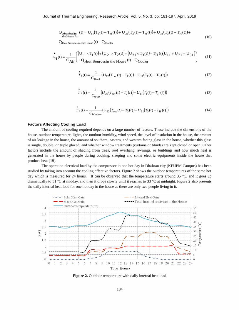
The operation electrical load by the compressor in one hot day in Dhahran city (KFUPM Campus) has been

studied by taking into account the cooling effective factors. Figure 2 shows the outdoor temperatures of the same hot

day which is measured for 24 hours. It can be observed that the temperature starts around 35 oC, and it goes up

dramatically to 51 oC at midday, and then it drops slowly until it reaches to 33 oC at midnight. Figure 2 also presents

the daily internal heat load for one hot day in the house as there are only two people living in it.

Figure 2. Outdoor temperature with daily internal heat load


185

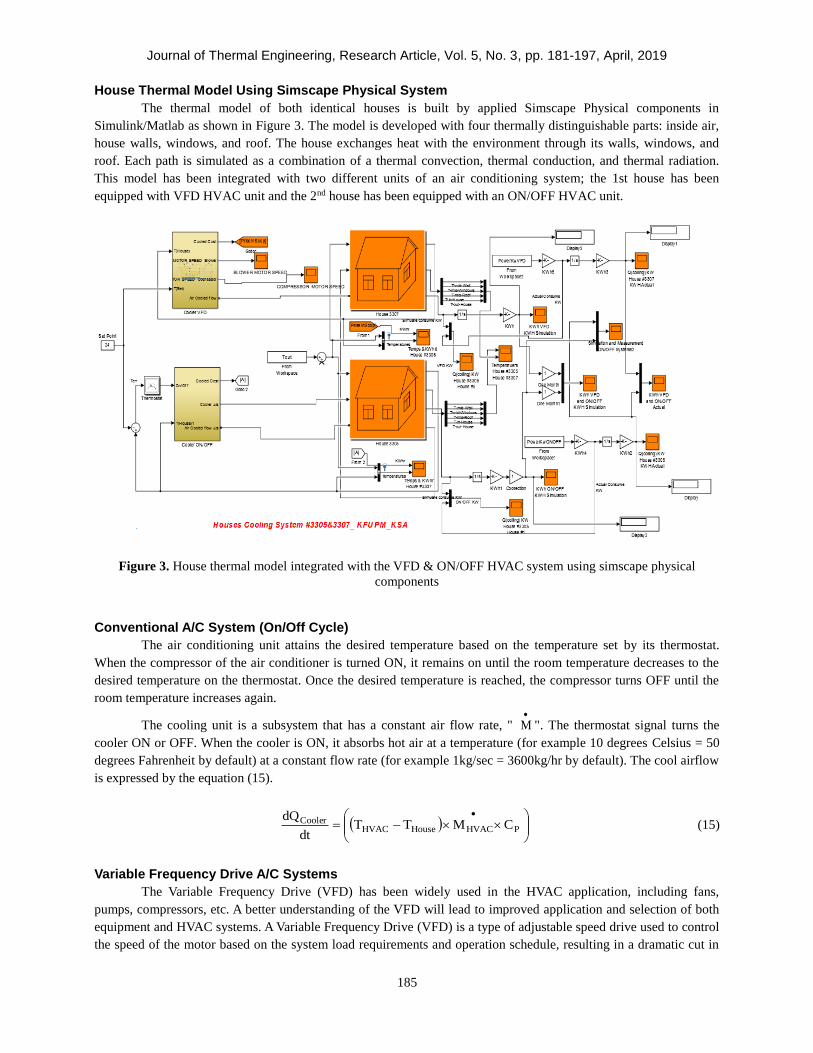
House Thermal Model Using Simscape Physical System

The thermal model of both identical houses is built by applied Simscape Physical components in

Simulink/Matlab as shown in Figure 3. The model is developed with four thermally distinguishable parts: inside air,

house walls, windows, and roof. The house exchanges heat with the environment through its walls, windows, and

roof. Each path is simulated as a combination of a thermal convection, thermal conduction, and thermal radiation.

This model has been integrated with two different units of an air conditioning system; the 1st house has been

equipped with VFD HVAC unit and the 2nd house has been equipped with an ON/OFF HVAC unit.

Figure 3. House thermal model integrated with the VFD & ON/OFF HVAC system using simscape physical

components

Conventional A/C System (On/Off Cycle)

The air conditioning unit attains the desired temperature based on the temperature set by its thermostat.

When the compressor of the air conditioner is turned ON, it remains on until the room temperature decreases to the

desired temperature on the thermostat. Once the desired temperature is reached, the compressor turns OFF until the

room temperature increases again.

The cooling unit is a subsystem that has a constant air flow rate, "

M ". The thermostat signal turns the

cooler ON or OFF. When the cooler is ON, it absorbs hot air at a temperature (for example 10 degrees Celsius = 50

degrees Fahrenheit by default) at a constant flow rate (for example 1kg/sec = 3600kg/hr by default). The cool airflow

is expressed by the equation (15).

PHVACHouseHVACCooler CMTTdt

dQ (15)

Variable Frequency Drive A/C Systems The Variable Frequency Drive (VFD) has been widely used in the HVAC application, including fans,

pumps, compressors, etc. A better understanding of the VFD will lead to improved application and selection of both

equipment and HVAC systems. A Variable Frequency Drive (VFD) is a type of adjustable speed drive used to control

the speed of the motor based on the system load requirements and operation schedule, resulting in a dramatic cut in


186

energy consumption [20]. VFD technology allows the air conditioner to automatically vary its power output to

specifically maintain room temperature at a desired or comfortable level. A non-inverter appliance maintains the

temperature by repeatedly switching the power ON and OFF, which consumes much more electrical energy upon

starting.

The VFD cooler has two options; constant value and variable air flow rate, " (t)MHVAC

". Based on equation

16, the variable airflow rate is delivered from the cooler system using a PI system. The air specific heat is multiplied

with airflow rate to produce cooler gain by equation 17. The HVAC coil temperature ( HVACT ) uses variable values

that are controlled by the PI system. Equation 18 is used to calculate the absorbed heat by the air in the house. In the

second subsystem equation 19, HouseT and SettingT are the inputs signal for the HVAC coil temperature subsystem and

the cooling air flow subsystem. The cooling airflows ( CoolerQ ) into the house are produced from the difference

between indoor temperature ( HouseT ) and the HVAC coil temperature ( HVACT ) and then multiplied by cooling gain.

(t)TKdt

(t))Td(TKM House1

Housesetting

0HVAC

(16)

PHVAC C(t)MGain(t)Cooler

(17)

)())((

32 tTKdt

tTTdKT House

HousesettingHVAC

(18)

Gain(t)Cooler TTdt

dQHVACHouse

Cooler (19)

EXPERIMENTAL ANALYSIS

Experimental Setup

The major role of the experimental work in this study is to confirm the validly of the simulation work, and

to evaluate the performance and energy consumption of the A/C systems. The monitoring and measurement hardware

system is comprised of four major blocks: two 5-ton Al-Zamil rooftop units, a Data Acquisition (DAQ) chassis with

National Instrument modules (Lab-View), sensors, and a host computer. The National Instrument DAQ-chassis

monitoring system has several modules such as voltage measurements, current measurements, and thermocouples.

There are four thermocouple sensors (three sensors for indoor and one for outdoor temperature), two humidity

sensors (indoor and outdoor), an irradiation sensor, barometric pressure sensor, and three air flow sensors. The host

computer has the National Instrument (NI) software, which is the main communicator with DAQ-chassis. The host

computer will initiate the execution commands, store the data and display them on the monitor.

Experiment Procedures

The experiments were conducted in the Guest Houses in KFUPM campus, Dhahran, Saudi Arabia. The floor

plan and the duct plan are shown in Figure 5.a. Each house consists of two rooms (one living room and one

bedroom), kitchen and bathroom. Moreover, all details of the houses which are integrated with ON/OFF and VFD

HVAC systems are described in this section and followed by a HVAC monitoring and measurement system.


187

Sensors Location in the Houses

Different types of sensors have been chosen and placed in both houses to read and measure the required data

for the experiment, Figure 4.b, and provide the location of each sensor in the house. Three thermocouple sensors are

fixed in the bedroom, corridor and living room. The temperatures are measured from three positions and then we

take the average temperature for a house. Airflow sensors are located near inlet air ducts to measure A/C unit flow in

kilogram per second. A pressure sensor is also placed inside the house to measure in-house pressure. A thermocouple

sensor and an irradiation sensor are placed on the roof of the house to measure the ambient temperature in degree and

daily irradiation in watt per meter square.

(a) (b)

Figure 4. (a) Floor plan for both houses, (b) Ducts plan and sensor’s locations in the houses

Monitoring and Measurement Systems

The monitoring and measurement systems for both units have been developed to achieve different tasks

such as displaying several physical and electrical characteristics, as well as environmental conditions. Furthermore,

the data acquisition systems incorporate signals, sensors, actuators, signal conditioning, data acquisition devices, and

application software. The purpose of data acquisition system is to measure the electrical or physical parameters such

as voltage, current, temperature irradiation, humidity, pressure, and wind speed. The PC-based data acquisition

system uses a combination of modular hardware, application software (Lab-View), and a computer to take

measurements [21]. Figure 5 shows the drawing map of the monitoring and measurement system.

In

HVAC System

Host Computer

Lab-View

3-Phase AC

Source

Out

Digital

Model

Thermal Couple

SensorsUniversal Model

NI9225,

4- Channel

NI9227,

4- Channel

Air Flow

Sensor

Out In

Irradiation

Sensor

Humidity

Outdoor SensorCTsPTs

OutIn

Humidity

Indoor Sensor

Figure 5. HVAC monitoring and measurement system


188

The superimposed graph displayed in Figure 6.a shows the instantaneous values of four temperatures and

pressure with time and Figure 6.b displays the instantaneous values (peak to peak) of line voltage with corresponding

RMS values.

Figure 6. (a), (b), Monitoring and measurement system (Lab-View Platform)

RESULTS AND DISCUSSION

In this section, the results for the simulation model with validation against the measuring data are provided

and the monthly results for variations of the energy consumption, energy savings, and COP variation have been

expressed. In addition, the cost analysis of both the ON/OFF and the VFD HVAC system with payback period for

each unit have been calculated.

Validation of the Simulation Results with Measurement Data for Both HVAC Systems

Simulation results for in-house air temperature and power consumption for one typical day, with normal

activities, (9th of April 2016) have been presented using Simulink/Matlab. The normal internal activities of the house

are shown in the Figure 2. The simulation results are produced for ON/OFF and VFD air conditioning units.

Measurement data are collected by Lab-View program for both residential houses. These data are validated with the

simulation results for both in-house air temperature and power consumption. Set point temperature is 24 oC with a

threshold (+1 oC & -1.5 oC) and the initial house air temperature is 24.1 oC.

Typical Day Activities (April 9, 2016) for the On/Off Cycle A/C Unit

Typical day activities validation for indoor temperature is shown in Figure 7. Simulated results are closely

following the measurement results where the number of pulses is also equal to 53. The average cycle period is also

identical, and the ON-time operation obtained by simulation and measurement are the same (451.05 min = 7.5175 h).

The outdoor air temperature affects directly the ON/OFF A/C unit as well as the ON pulse numbers. The outdoor

temperature as shown in Figure 7 is still constant and equal to 23 oC from midnight to 6:00 AM and then it

increases dramatically to 42.5 oC at 12:30 PM. The temperature decreases again slowly to reach 27.5 oC at 7:30 PM.

The house has permanent activities (fridge, computer, monitor, Wi-Fi, lights, and printer) and variable activities

(cooking, washing machine, open/close door and windows, etc.).

The activities of heat losses begin at 1.087 kW and goes up to reach 1.27 kW. Then it goes down to 0.87kW

as the outdoor temperature stays at 23 oC. From 2:30 AM to 4:00 AM, a decrease is observed in duty cycle that is

affected by outdoor temperature reduction to 21oC as well as a reduction in in-house activities. While the outdoor

temperature increases from 05:30 AM to 10:00 AM, the duty cycle is still low, and it is affected directly by the tree’s

shadow that is close to the east window of the house. From 10:00 AM to 6:00 PM, the ON/OFF frequency increases

due to the increase in the outdoor temperature that reaches 42.5 oC at midday. The social activities (lunch, dinner,

washing machine, open/close windows and door, etc.), increase the duty cycle. The ON/OFF frequency again

(a) (b)


189

decreases slowly as a result of the outdoor temperature reduction to 26 oC and some of the social activities (cooking

dinner, boiling tea water, etc.), so the duty cycle decreases slowly again.

The simulation and the measurement of the power consumption for the ON/OFF cycle unit on April 9, 2016

are presented in Figure 8. The simulated results are similar to the measurement results (4.95 kW rated value), where

the number of the ON/OFF pulses are also equal (53 pulses). The OFF time is (989.112 min = 16.4852 h). The

outdoor temperature shown in Figure 7 went up at 10:00 AM to 32 oC and reached 42.5 oC at 12:30 PM. This causes

the condenser of the A/C unit to start increasing the power consumption. The total power reached to 5.4 kW when the

condenser of the A/C unit is connected directly with the compressor supply. On the other hand, when the outdoor

temperature reaches 27.5 oC, the compressor A/C unit temperature decreases so the condenser power consumption

also decreases. In this case, the total power reaches the nominal power of 4.95 kW.

Figure 7. Measured and simulated indoor temperature and the outdoor temperature on 9th of April 2016

Figure 8. Measured and simulated consuming power for the ON/OFF cycle A/C unit on the 9th of April 2016


190

Typical Activities (April 9, 2016) for the VFD A/C Unit

Similarly, the typical activities validation for the indoor temperature is displayed in Figure 9. The simulated

results are similar to those of the measurement, where the temperature for both values is in the same level (24.5 oC to

23 oC). The outdoor temperature and typical activities (permanent and social heat load) have a direct effect on the

VFD A/C unit performance, where the amount of flow rate is increased or decreased to match closely the set point

temperature (24 oC).

The simulation and measurement of the power consumption for the VFD A/C unit on the 9th of April, 2016

are shown in Figure 10. The power consumption starts to rise at 05:30 AM and reaches a maximum value (1.7 kW)

at 10:00 AM until 12:00 PM because of the in-house activities (cooking breakfast/lunch, washing machine,

open/close windows and door, etc.), and rise in the outdoor temperature. The power consumption decreases gradually

until it reaches 0.9 kW at 3:00 PM and increases again to 1.3 kW because of the increase in the in-house activities

(cooking dinner, washing machine, open/close door, boiling tea water, etc.). It then goes down to 0.4 kW till 09:00

PM and finally goes up to 0.9 kW at midnight.

Figure 9. Outdoor measured temperature and indoor measured temperature and indoor simulated temperatures by

the VFD HVAC unit on the 9th of April, 2016

Figure 10. Measured and simulated power consumption for the VFD A/C unit on the 9th of April, 2016


191

Energy Analysis for Both On/Off Cycle and VFD HVACSystems

The energy consumption for the ON/OFF cycle and the VFD HVAC units is calculated by integrating the

area under power consumption curve as shown in Figures 8 & 10 for typical activities (9 th of April, 2016) for both

simulation results and data measurement. Table 1 shows the energy consumption of both ON/OFF and VFD HAVC

for one typical day.

Table 1. Energy analysis for the ON/OFF cycle and the VFD HVAC systems for one day

Day

Simulated Results Measurement Data

ON/OFF Cycle Unit

(kWh)

VFD Unit

(kWh)

Saving

%

ON/OFF Cycle

Unit (kWh)

VFD Unit

(kWh)

Saving

%

Typical activities

(April 9, 2016) 37.212 22.4 39.53 38.44 23.71 38.31

A summary of measured energy consumption for two months (April 2016 and May 2016) that is used for

the validation of the simulation results is presented in Table 2. The comparison of the energy consumption for the

ON/OFF cycle and the VFD HVAC units and energy savings are also presented in the Table.

Table 2. Comparison energy consumption for the ON/OFF cycle and the VFD HVAC systems for two months, 2016

Months

Simulated Results Measurement Data

ON/OFF Cycle Unit

(kWh)

VFD Unit

(kWh)

Saving

(%)

ON/OFF Cycle Unit

(kWh)

VFD Unit

(kWh)

Saving

%

April 1042.058 571.0345 45.2012 1098.3 519.3 52.7184

May 1763.567 1038.548 41.1109 1606.11 1130.88 29.589

Monthly Variation of Energy Consumption

Table 3 presents a summary of the results of energy consumption for seven months of study. Both the

ON/OFF cycle HVAC and the VFD HVAC systems are used with the same conditions. The average operation

period of the ON/OFF cycle and the number of ON pulse also are displayed in the table. The energy consumption in

kW is presented for both the ON/OFF cycle and the VFD HVAC systems. The hottest months, June and July, show

the higher duty cycle per month. The comparison of the energy consumption for both systems is shown in Figure 11

and the energy savings per month is presented in Figure 12. Table 3 shows that a considerable amount of savings of

energy occur from April 2016 to Oct. 2016.

Table 3. Comparison energy used for the ON/OFF and the VFD HVAC systems for several months

Months

ON/OFF Cycle HVAC System VFD HVAC System

Numbers

of (ON)

Pulses

The

average of

ON Time

(mins)

The

average of

OFF Time

(mins)

The

average

ON Duty

Cycle (%)

Energy

used per

Month

(kWh)

Energy

used per

Month

(kWh)

Energy

Saving

(%)

April 2016 1450 7.0172 16.982 50.342 1042.058 571.0345 45.2012

May 2016 1906 11.492 12.507 53.072 1763.567 1038.548 41.1109

June 2016 2190 13.500 10.499 54.15 2004.897 1329.972 33.6638

July 2016 2309 13.796 10.203 54.380 2117.09 1419.172 32.9659

Aug. 2016 2208 13.046 10.953 53.166 2002.028 1326.967 33.7188

Table 3. (Cont.) Comparison energy used for the ON/OFF and the VFD HVAC systems for several months


192

Months

ON/OFF Cycle HVAC System VFD HVAC System

Numbers

of (ON)

Pulses

The

average of

ON Time

(mins)

The

average of

OFF Time

(mins)

The

average

ON Duty

Cycle (%)

Energy

used per

Month

(kWh)

Energy

used per

Month

(kWh)

Energy

Saving

(%)

Sep. 2016 2150 11.732 12.267 53.333 1742.216 1142.922 34.3983

Oct. 2016 1540 7.9502 16.049 51.633 1219.962 756.8483 37.9613

Figure 11. Energy consumption for the ON/OFF cycle and the VFD HVAC system

Monthly Energy Savings

The energy consumption is the power (P) multiplied with the time of operation (t) of the AC system [22],

whereas the percentage of energy savings is calculated based on the difference between energy consumed using the

ON/OFF control and energy consumed using the VFD control.

(kW)1000

PFIVPower

(20)

where I is the current (Ampere), V is voltage (Volts), and PF is the power factor.

(kWh)t PowerEnergy (21)

100Energy HVAC ON/OFF

Energy] HVAC VFD[Energy HVAC ON/OFFSavingsEnergy

(22)

The energy savings per month is shown in Figure 12.


193

Figure 12. Energy saving rate per month

Average Monthly COP Variations

The coefficient of performance (COP) is commonly used to express the efficiency of an air-conditioning

system [22]. The main purpose of the A/C system is to remove heat or to process load from the evaporator ( LQ ).

The energy required at the compressor ( comW ) is to accomplish the refrigeration effect. Thus, the COP is expressed

as:

(kWh)n ConsumptioEnergy Total

(kWh) Input)(Energy Gain Heat Internal

comW

LQ

1h2h

4h1hCOP

(23)

where, 1h and 2h (kJ/kg) are the enthalpy at the compressor inlet and that of the compressor outlet, respectively, 4h

(kJ/kg) is the enthalpy at the evaporator inlet, LQ (kWh) is the refrigerating effect, and comW (kWh) is the

compression work.

The maximum theoretical COP for the air conditioning system is expressed by Carnot’s theorem given by

the following equation:

CTHT

CT

MaximumCOP

(24)

where CT is the cold temperature and HT is the hot temperature. The air conditioning system cools the house to

22.5 oC for (ON/OFF) and 24 oC for (VFD). If the average outdoor temperature is 35.55 oC the theoretical maximum

COP is:

1.72=

CTHT

CT

OFFONMaxCOP

(25)


194

2.10=

CTHT

CT

MaxCOPVFD

(26)

The total internal heat gain for the 9th of April 2016 is calculated based on the solar heat gain, mass heat

gain, and the internal house activities in both houses. On the other hand, the monthly average COP variation is

calculated based in the measured energy and the internal Heat Gain (April 2016).

The daily average of internal Heat Gain for the month of April for both houses = 42.922 kWh

The daily average of energy used for the month of April by the ON/OFF HVAC unit = 36.61 kWh

The daily average of energy used for the month of April by the VFD HVAC unit = 20.82 kWh

1.172kWh 36.61

kWh 42.922

W

QCOP

com

LOFFON (27)

2.062kWh 20.82

kWh 42.922

W

QCOP

com

LVFD (28)

Cost Analysis of Both the On/Off and the VFD HVAC System

The payback period is calculated by counting the number of years it will take to recover the cash invested in

installing the VFD HVAC unit instead of the conventional ON/OF HVAC unit. The payback period for setting the

temperature to 24 oC can be calculated by the following formula.

Saving Annual

Cost AdditionalPeriodPayback (29)

The cost difference between the ON/OFF unit and the VFD unit is about 40% (8750SR) in which the VFD

unit is higher cost than the conventional ON/OFF unit.

Based on the calculation performed in Table 4, the payback period is six years and 6 months, so if the user

installs a VFD HVAC system, he can recover the extra paid money within 6 years and 6 months. During the time

after the payback period, the user will start to get the benefit of having the VFD HVAC in the house as the energy

consumption is going to be less than that of having an ON/OFF unit.

Table 4. Payback period for a residential HVAC

Electrical Energy Cost [23] Annual Consumption

Residential Sector

ON/OFF VFD

Annual

Energy

Savings

Annual Cost

Saving

Payback

Years kWh Halalah

1-2000 5

2001-4000 10

4001-6000 20

6001- 8000 30

4 8734.92

kWh

34%

4481.484

kWh

4481.484 kWh* 0.3

Hala=1325.54SR

6 years

&

6 months

8000 < 30

CONCLUSIONS

The HVAC systems incorporating the ON/OFF controller and the VFD controller are considered to

determine the compressor power consumptions for the HVAC unit in residential areas located at the King Fahd

University of Petroleum and Minerals campus in the Kingdom of Saudi Arabia. Thermal analysis is carried out in


195

line with the experimental conditions to assess the energy consumption of the HVAC system. The experimental set-

up is developed incorporating the LabVIEW based data acquisition monitoring and measurement system. The

thermal model considers different types of A/C system controller (ON/OFF, VFD) units. The predictions of the

power consumptions of the HVAC system have been compared with those of the measured data. The developed

mathematical thermal house model is integrated with the cooling source model of an ON/OFF cycle and VFD air

conditioning systems. The developed thermal models are simulated by using Simscape physical components in

Matlab/Simulink environment. In addition, the analysis pertinent to the assessment of energy consumptions, energy

savings, and the cost of the payback period have been evaluated. In general, the variable frequency drive controller

provides higher efficiency and low cost of A/C system. In addition, the specific conclusions derived from the present

study are listed as follows:

The energy consumptions have been examined for several months and it is demonstrated that the energy

savings reach between 32% - 45% during the period from April 2016 to October 2016. It has been noticed that

the performance system simulation is affected by the outdoor temperature and the indoor activities during the

day. Energy savings with VFD reached 45% in a medium outdoor temperature.

The simulation results matched significantly with the experimental data measurement with an error of about

3%.

The daily and monthly average COP variations of actual and ideal system are calculated and the findings

revealed that VFD unit has higher COP than the ON/OFF cycle.

The cost analysis and the payback period have been calculated. It is found that the user needs only 6 years and

a half to recover the additional cost. In the near future, if there is any further drop in the price of the VFD unit,

it will become a catalyst in the promotion of energy conversion through the use of a VFD unit.

The paper has shown that installing a VFD for a residential HVAC system gives considerable energy savings

over the ON/OFF cycle.

ACKNOWLEDGMENT The authors acknowledge the support by the DSR funded project RG1205-1&2 at King Fahd University of

Petroleum and Minerals, Dhahran, Saudi Arabia for this research work. Also, the authors acknowledge the donation

of two 5-tons A/C systems from the Al-Zamil Air-Conditioning Company, Industrial City, Dammam, Saudi Arabia.

NOMENCLATURE H Heat transfer coefficient, W/m2.K

Tout External house temperature, K

TH Internal house temperature, K

T1 Internal roof temperature, K

T2 Internal wall temperature, K

T3 Internal windows temperature, K

CAir Specific heat of air, J/kg

CRoof Specific heat of roof, J/kg

CWall Specific heat of wall, J/kg

CWind Specific heat of window, J/kg

QAir The rate of energy stored in the volumetric space of the house, J

QRoof The rate of energy stored in the wall, J

QWall The rate of energy stored in the roof, J

QWind The rate of energy store in the windows, J

(t)MHVAC

Mass flow rate of supply air, kg/s

CP Air specific heat, J/kg. K

THouse In-House temperature, K

THVAC HVAC coil A/C temperature, K

K0 The effective cooler gain, kg/K (default 0K = 1 kg/K)

K1 The effective time cooler gain, kg/s.K (default 1K = 1 kg/s. K)

K2 The effective HVAC gain, default 2K = 0.005


196

K3 The effective time HVAC gain, 1S(default 3K = 0.9

1S)

dt

dQCooler The absorbed heat flow rate by cooler, J/s

SourceHouseHeatQ The heat source, J

REFERENCES [1] Salmi, W., Vanttola, J., Elg, M., Kuosa, M., Lahdelma, R. (2017). Using waste heat of ship as energy source for

an absorption refrigeration system. Applied Thermal Engineering, 115, 501-516.

[2] Aly, W. I., Abdo, M., Bedair, G., Hassaneen, A. E. (2017). Thermal performance of a diffusion absorption

refrigeration system driven by waste heat from diesel engine exhaust gases. Applied Thermal Engineering, 114, 621-

630.

[3] Wang, J., Wang, B., Wu, W., Li, X., Shi, W. (2016). Performance analysis of an absorption-compression hybrid

refrigeration system recovering condensation heat for generation. Applied Thermal Engineering, 108, 54-65.

[4] Xu, Y., Jiang, N., Wang, Q., Chen, G. (2016). Comparative study on the energy performance of two different

absorption-compression refrigeration cycles driven by low-grade heat. Applied Thermal Engineering, 106, 33-41.

[5] Sun, L., Han, W., Jin, H. (2015). Energy and exergy investigation of a hybrid refrigeration system activated by

mid/low-temperature heat source. Applied Thermal Engineering, 91, 913-923.

[6] Farsi, A., Mohammadi, S. H., Ameri, M. (2017). Thermo-economic comparison of three configurations of

combined supercritical CO2 refrigeration and multi-effect desalination systems. Applied Thermal Engineering, 112,

855-870.

[7] Al-Shaalan, A., Ahmed, W., Alohaly, A. (2014). Design guidelines for buildings in Saudi Arabia considering

energy conservation requirements. In Applied Mechanics and Materials (Vol. 548, pp. 1601-1606). Trans Tech

Publications.

[8] Salsbury, T., Diamond, R. (2000). Performance validation and energy analysis of HVAC systems using

simulation. Energy and buildings, 32(1), 5-17.

[9] Muratori, M., Marano, V., Sioshansi, R., Rizzoni, G. (2012, July). Energy consumption of residential HVAC

systems: a simple physically-based model. In 2012 IEEE Power and Energy Society General Meeting (pp. 1-8).

IEEE.

[10] Karmacharya, S., Putrus, G., Underwood, C., Mahkamov, K. (2012, June). Thermal modelling of the building

and its HVAC system using Matlab/Simulink. In 2012 2nd International Symposium On Environment Friendly

Energies And Applications (pp. 202-206). IEEE.

[11] Wen, Y., Burke, W. (2013, April). Real-time dynamic house thermal model identification for predicting HVAC

energy consumption. In 2013 IEEE Green Technologies Conference (GreenTech) (pp. 367-372). IEEE.

[12] Zhu, Y. (2006). Applying computer-based simulation to energy auditing: A case study. Energy and

buildings, 38(5), 421-428.

[13] Zhou, D., Park, S. H. (2012). Simulation-assisted management and control over building energy efficiency–a

case study. Energy Procedia, 14, 592-600.

[14] Yu, J., Yang, C., Tian, L. (2008). Low-energy envelope design of residential building in hot summer and cold

winter zone in China. Energy and Buildings, 40(8), 1536-1546.

[15] Nasution, H., Dahlan, A. A., Aziz, A. A., Azmi, U., Sumeru, S., Shodiya, S. (2016). Energy Efficiency of A

Variable Speed of The Centralized Air Conditioning System Using PID Controller. Jurnal Teknologi, 78(8-4).

[16] Coley, D. A., Penman, J. M. (1996). Simplified thermal response modelling in building energy management.

Paper III: Demonstration of a working controller. Building and environment, 31(2), 93-97.

[17] Hamanah,W.M., (2016), “Modeling, Simulation and Energy Performance of VFD and ON/OFF Cycle HVAC

Systems,” M.S. thesis, KFUPM, Az Zahran, Saudi Arabia.

[18] Hamanah, W. M., Kassas, M., Mokheimer, E. M., Ahmed, C. B., Said, S. A. M. (2019). Comparison of Energy

Consumption for Residential Thermal Models With Actual Measurements. Journal of Energy Resources

Technology, 141(3), 032002.


197

[19] Ohyama, K., Kondo, T. (2008). Energy‐ Saving Technologies for Inverter Air Conditioners. IEEJ Transactions

on Electrical and Electronic Engineering, 3(2), 183-189.

[20] Ohyama, K., Kondo, T. (2008). Energy‐ Saving Technologies for Inverter Air Conditioners. IEEJ Transactions

on Electrical and Electronic Engineering, 3(2), 183-189.

[21] Belhadj, C. A., Hamanah, W. M., Kassas, M. (2017, June). LabVIEW based real time Monitoring of HVAC

System for Residential Load. In 2017 IEEE International Conference on Computational Intelligence and Virtual

Environments for Measurement Systems and Applications (CIVEMSA) (pp. 66-71). IEEE.

[22] Affandi, M. (2004). Energy Saving in an Air-Conditioning System Using an Inverter and a Temperature-Speed

Controller (Doctoral dissertation, Universiti Teknologi Malaysia).

[23] Council of Ministers, (2016) Consumption Tariff, Saudi Electricity Company, No.95 https://www.se.com.sa/en

us/customers/Pages/TariffRates.aspx/

https://www.se.com.sa/en%20us/customers/Pages/TariffRates.aspx

https://www.se.com.sa/en%20us/customers/Pages/TariffRates.aspx

OPERATION OF HVAC SYSTEM FOR ENERGY SAVINGS AND …

Documents

Transcript of OPERATION OF HVAC SYSTEM FOR ENERGY SAVINGS AND …