Operating Leverage and Future Earnings · high operating leverage induces an asymmetric effect on...

1

Operating Leverage and Future Earnings

David Aboody

Anderson School of Management at UCLA

Shai Levi

The Faculty of Management, Tel Aviv University

Dan Weiss

The Faculty of Management, Tel Aviv University

Dec 7, 2014

Abstract

This study examines the impact of operating leverage, defined as the ratio between fixed and

variable costs, on future earnings. First, we find that high operating leverage has a longer impact

on future earnings than low operating leverage, primarily because of a slower cost-adjustment

process. Second, for firms with high operating leverage, a negative revenue shock has a larger

negative impact on future earnings than a positive revenue shock. That is, we document that

high operating leverage induces an asymmetric effect on future earnings, mainly driven by a

slower cost-adjustment process on the downside than on the upside. Examining the implications

of high operating leverage, we find that firms with high operating leverage hold low financial

leverage and pay their executives more equity-based compensation. Overall, our findings are an

important addition to two streams of studies: operating leverage and cost behavior.

Acknowledgments: The authors are grateful for constructive suggestions and helpful comments from Yacov

Amihud, Eli Amir, Ilan Cooper, Eti Einhorn, Efrat Shust, Tzahi Versano, Avi Wohl, and participants of the seminars

at Tel Aviv University and UCLA.

2

Operating Leverage and Future Earnings

1. Introduction

This study examines the effect of operating leverage, defined as the ratio between fixed and

variable costs (Lev, 1974; Balakrishnan et al., 2013) on future earnings. Microeconomic models

predict that high operating leverage leads to high earnings volatility. For example, the earnings

volatility of a firm with only fixed costs is equal to the firm’s revenue volatility, and for the same

firm with some variable costs and similar revenue volatility, earnings volatility is relatively

lower. Firms can adjust some costs in response to revenue shocks, but adjusting other costs may

be difficult in the short run. Whereas some recent studies document an immediate cost response

to revenue shocks (e.g., Chen et al., 2012; Banker et al., 2013), we examine whether operating

leverage, an outcome of a cost structure choice, has a long-lasting impact on earnings.

Investigating the enduring relationship between operating leverage and future earnings, we

also examine whether operating leverage affects future earnings growth symmetrically under

favorable versus unfavorable revenue shocks. Whether operating leverage should affect future

earnings growth symmetrically is unclear. On one hand, microeconomics and management

accounting textbooks usually entertain a linear fixed-variable cost model, suggesting a

symmetrical reaction to favorable and unfavorable revenue shocks (Garrison et al., 2012;

Horngren et al., 2013). On the other hand, prior studies following Anderson et al. (2003)

documented a contemporaneous asymmetric cost response to revenue shocks - costs decrease

less when revenue falls than they increase when revenue rises by an equivalent amount. Later

studies showed the resulting contemporaneous earnings asymmetry - earnings decease more

when revenue falls than they increase when revenue rises by an equivalent amount (Anderson et

al., 2007; Weiss, 2010; Kama and Weiss, 2013; Banker and Byzalov, 2014). However, the

literature has not yet explored the potentially asymmetric impact of operating leverage on the

earnings-adjustment process over a long period. Because firms with high operating leverage have

difficulty adjusting resources in the short run, one would expect ongoing cost- and earnings-

adjustment processes for firms with high operating leverage. Addressing this void, we investigate

the length of the response period by testing the enduring association between operating leverage

and earnings growth. Allowing for a differential cost response between favorable and

unfavorable revenue shocks, our empirical tests separate the sample into revenue increases and

3

decreases to provide means for testing a long-lasting asymmetric impact of operating leverage on

future earnings.

Results are based on a sample of 80,290 firm-year observations from 1961 to 2012. We adopt

Lev’s (1974) operating leverage measure, which uses a long time series of eight years.1 Findings

show that firms with higher operating leverage (i.e., more fixed costs and less variable costs)

experience a greater increase in earnings in the three years following a positive revenue shock

and a greater decrease in earnings in the three years following a negative revenue shock. These

results are consistent with the prevalent assertion that high operating leverage increases earnings

volatility. Importantly, we show that slow cost adjustments drive the slow earnings-adjustment

process for high-operating-leverage firms. Overall, the findings for firms with high operating

leverage suggest a slow and ongoing adjustment process over three subsequent years, above and

beyond an immediate response to revenue shocks documented in prior studies.

Notably, the results suggest the long-lasting operating leverage effect on earnings growth is

asymmetric. Specifically, for high-operating-leverage firms, we find that future earnings increase

less when revenue rises than they decrease when revenue falls in the three subsequent years. That

is, the impact of high operating leverage on future earnings is more pronounced on the downside

than on the upside. We also find that costs, not revenue, are the main cause of this asymmetry.

These findings suggest the long-term cost-adjustment process of firms with high operating

leverage leads to enduring asymmetric earnings behavior.

Results from performing a battery of context analyses reconfirm the findings and offer

further insights. First, we demonstrate that the results are prominent in the pharmaceutical

industry, which is characterized by the highest operating leverage. By contrast, we document a

marginal effect for retailers, characterized by the lowest operating leverage. Second, we

document that high operating leverage provides means for taking advantage of a prosperous

economy, whereas low operating leverage is expedient for promptly adjusting resources when

the economy takes a downturn. Third, evidence from replicating the analyses for subsamples

with two consecutive favorable versus unfavorable revenue shocks further corroborates the

findings. In sum, we find that (i) operating leverage has a long-lasting effect on future earnings

for up to three years because of a gradual cost-adjustment process, which boosts earnings

1 Using a long time series introduces a selection bias toward mature firms.

4

volatility, and (ii) operating leverage has an asymmetric impact on future earnings: future

earnings increase less when revenue rises than they decrease when revenue falls.

Furthermore, we provide additional subtle insights on the costs and benefits of operating

leverage. Such analyses are noteworthy given our findings that the outcome of a negative

revenue shock is more severe than the benefits from a positive revenue shock for high-operating-

leverage firms. We document two reasons for adopting high operating leverage: (i) revenue

increases are much more prevalent than revenue decreases (71.5% to 28.5%), and high operating

leverage provides a means for taking advantage of increasing demand and prosperous periods,

and (ii) firms adopt high operating leverage because of having financial leverage constraints

(Kahl et al., 2013).

Finally, high operating leverage, in spite of the benefits to shareholders, imposes a burden on

risk-averse managers that dislike high earnings volatility and low performance levels when

revenue falls or the economy takes a downturn. In our final analysis, we find that high operating

leverage is associated with higher equity-based compensation costs. Because option value

increases with volatility and its downside is protected, shareholders that prefer high operating

leverage will increase the use of options to incentivize managers to choose high operating

leverage.

Our paper contributes as follows. First, the results expand our understanding of how

operating leverage influences the length of firms’ earnings adjustment period in response to

demand shocks. Our results indicate that contrary to earlier studies that view cost-adjustment

processes as short-term phenomena, we find that cost-adjustment processes in high-operating-

leverage firms last over three years. That is, operating leverage influences firm earnings three

years ahead, particularly when revenue falls.

Second, the documented asymmetry shows that high operating leverage adds an operational

constraint on firm responses to unfavorable demand shocks. On the other hand, high operating

leverage provides a means of taking advantage of favorable demand shocks. These findings add

an important dimension to the operating leverage literature (Lev, 1974; Kallapur and Eldenburg,

2005; Kahl et al., 2013; Banker et al., 2014).

Finally, our paper also contributes to the sticky cost literature, which documents an

immediate asymmetric cost response to revenue shocks. We document asymmetric cost behavior

driven by high fixed costs. Our evidence links operating leverage with cost stickiness.

5

Specifically, cost stickiness is more pronounced for high-operating-leverage firms than for low-

operating-leverage firms because adjusting resources is more difficult for high-operating-

leverage firms. Moreover, the stickiness phenomenon continues beyond the year of the revenue

shock and affects earnings in subsequent years, particularly for high-operating-leverage firms.

The remaining sections of this paper are organized as follows: Section 2 lays out the

hypotheses, Section 3 describes the research design for estimating operating leverage, Section 4

presents the main empirical findings, Section 5 adds contextual analyses, Section 6 presents

insights on costs and benefits of operating leverage, and Section 7 concludes.

2. Hypotheses and Literature Review

Operating leverage reflects the proportion of fixed costs in a firm’s cost structure. High

operating leverage, that is a high proportion of fixed costs to variable costs, results in high

sensitivity of profits to changes in activity level and a high break-even point. Firms with high

operating leverage tend to have high profit margins, where a change in activity level has a large

impact on earnings (Lanen et al., 2013). Although numerous studies explore various aspects of

firms’ financial leverage, literature focusing on operating leverage is limited.

In an early study, Lev (1974) associates operating leverage and risk. He shows that operating

leverage increases both the overall and systematic risk. Kallapur and Eldenburg (2005) report

that uncertainty leads firms to prefer technologies with low operating leverage; i.e., low fixed

and high variable costs. Recently, Novy-Marks (2010) documents that operating leverage

predicts returns in the cross section. Both Lev and Novy-Marks argue that operating leverage is

associated with a value premium.

Prior studies have also investigated a relationship between operating leverage and financial

leverage, suggesting substitution between the two leverages. Van Horne (1977) argues that firms

with high operating leverage choose low financial leverage. Mandelker and Rhee (1984)

demonstrate how operating leverage contributes to systematic risk above and beyond financial

leverage, in support of Van Horne’s argument. Recently, Kahl et al. (2013) show that firms with

high operating leverage have low financial leverage but also large cash holdings.

Taking a different perspective, operating leverage is a fundamental concept in management

accounting. Textbooks assert that high operating leverage leads to high earnings volatility and a

6

high break-even point (Garrison et al., 2012; Horngren et al., 2013). Although this assertion is

widely taught, it has not been empirically validated. Particularly, prior studies have not yet

examined the relationship between operating leverage and future profitability.

Some prior studies report an immediate cost response to revenue shocks (e.g., Chen et al.,

2012; Banker et al., 2013; Cannon, 2014). However, these studies cannot speak to whether the

adjustment process is fully completed within the concurrent year. Therefore, the adjustment

process might continue over time.

Addressing the length of the cost-adjustment process, we note that firms make long-term

commitments in acquiring capacity, resulting in fixed costs. Fixed costs arise from the

possession of facilities, infrastructure, machines, and equipment and from retaining experienced

and skilled personnel. The fixed costs include property taxes, lease payments, depreciation,

insurance, and salaries of key personnel. These fixed costs are slowly modified because of their

high cost of adjustment. Specifically, an adjustment process is spread over a long period in

response to revenue shocks, both revenue increases and revenue decreases. Therefore, we

examine whether operating leverage has a long-lasting impact on earnings.

Hypothesis 1

Operating leverage has a positive (negative) long-lasting effect on future profitability when

revenue rises (falls).

Operating leverage is commonly measured by the ratio between fixed and variable costs

(Lev, 1974; Balakrishnan et al., 2013; Banker et al., 2014).2 Although the fixed-variable cost

model underlying the operating-leverage concept implies a linear and symmetric cost structure,

Anderson et al. (2003) and a large body of subsequent studies document cost asymmetry - costs

increase more when revenue rises than they decrease when revenue falls by an equivalent

amount. The literature explores various immediate managerial responses to increases versus

decreases in revenue resulting in asymmetric costs.3

2 Taking a different path, Novy-Marks (2010) measures operating leverage in a different context. He measures

firms’ operating costs relative to their capital stocks, not the ratio of fixed to variable costs. 3 See, e.g., Balakrishnan et al. (2004), Balakrishnan and Gruca (2008), Chen et al. (2012), Dierynck et al. (2012),

Banker et al. (2013), Kama and Weiss (2013), Cannon (2014), Holzhacker et al. (2014), Banker et al. (2014), and

Shust and Weiss (2014). Banker and Byzalov (2014) offer a review of the asymmetric costs literature.

7

More importantly, asymmetric costs result in earnings asymmetry - earnings increase less

when revenue rises than they decrease when revenue falls by an equivalent amount (Anderson et

al., 2007; Weiss 2010). Banker and Chen (2006) use the earnings-returns relationship for

documenting that both fixed-variable costs and asymmetric costs have one-year-ahead predictive

power with respect to stock prices. That is, past choices of cost structures influence stock prices

one year ahead.

Considering a long-lasting impact of operating leverage on future earnings, we have in mind

a capacity choice, which is a choice made in advance, before demand is realized. Capacity

choices influence a firm’s cost structure, which, in turn, determines its operating leverage. In

other words, the level of capacity utilization is likely to affect the extent of cost asymmetry

(Balakrishnan et al., 2004), and, in turn, the level of future earnings asymmetry. Under high

capacity utilization (strained capacity), a response to a revenue decrease would be lower than the

response to a revenue increase of an equivalent amount. Managers would use a revenue decrease

to relieve pressure on available resources and not reduce resource levels proportionately.

Conversely, a revenue increase is likely to cross resource thresholds and trigger a

disproportionate increase in resources. Therefore, capacity set in advance is expected to

influence cost asymmetry and, in turn, earnings asymmetry over an enduring process of cost

adjustment. This phenomenon is more influential in firms with intensive capital investments, that

is, a high proportion of fixed costs. Following this path, Shust and Weiss (2014) report that

depreciation enhances the extent of cost asymmetry. Again, firms with intensive capital

investments have more depreciation expenses, which induce greater costs and earnings

asymmetry over time. Therefore, high operating leverage determined in advance is likely to

induce future earnings asymmetry.

In a similar vein, Balakrishnan et al. (2013) argue that long-run cost-structure choices also

influence cost asymmetry. However, the empirical literature has not yet looked into the impact of

fixed-variable cost structures on the level of future earnings asymmetry. Overall, we expect to

find that operating leverage has an asymmetric impact on future earnings.

Hypothesis 2

Operating leverage has an asymmetric impact on future earnings: Future earnings increase less

when revenue rises than they decrease when revenue falls.

8

3. Estimating Operating Leverage, Sample, and Descriptive Statistics

3.1 Operating Leverage

Estimating operating leverage, Lev (1974) runs a time-series regression of costs on revenue

and uses the estimated coefficient on revenue as a measure of a firm’s operating leverage.4

Following the same path, Noreen and Soderstrom (1994), Banker et al. (1995), Noreen and

Soderstrom (1997), Kallapur and Eldenburg (2005) and Banker et al., (2014) use the log-linear

specification for estimating time-series regressions of costs on revenue. We build on these prior

studies by estimating the following time-series model for each firm i and year t:

OCi,k = α + βi,t REVi,k + i,k, k = t-8,…,t-1, (1)

where OC is the natural logarithm of total operating costs, estimated as revenue minus income

from operations. REV is the natural logarithm of revenue.5

As in Lev (1974), we use revenue as an imperfect proxy for the activity volume, because

activity volume levels are not observable. Employing revenue as a fundamental stochastic

variable for measuring activity levels is in line with Dechow et al. (1998), Kallapur and

Eldenburg (2005), and a number of sticky cost studies (e.g., Anderson et al., 2003; Banker and

Chen, 2006; Weiss, 2010). Prior studies use this specification because it is consistent with the

generalized Cobb-Douglas production function (see also Noreen and Soderstrom (1994) and

Banker et al. (1995)). In estimating regression model (1), we use windows of eight years of data

per firm.

To the extent that revenue is a reasonable proxy of actual activity volume, Noreen and

Soderstrom (1994) demonstrate that the coefficient β is the ratio of marginal to average costs.

Because the fixed-variable cost model underlying the operating-leverage measurement assumes

linearity, Kallapur and Eldenburg (2005) interpret the coefficient β as the proportion of variable

costs to total costs. For two firms, i=1,2, suppose VCi is the variable costs and FCi is the fixed

costs, and the estimated β1 < β2. We get

1 - β1 > 1 - β2, (2)

1 – (VC1/(VC1+FC1)) > 1 – (VC2/(VC2+FC2), (3)

Operating Leverage of firm 1 = FC1 / VC1 > Operating Leverage of firm 2 = FC2 / VC2 . (4)

4 Lev (1974) uses 20-year and 12-year windows for estimating the time-series regressions.

5 In addition, we replicate the analyses using values of the variables rather than the natural logarithm. The results are

essentially the same.

9

Because operating leverage is the ratio between fixed costs and variable costs, if 1 - β1 > 1 - β2,

the operating leverage of firm 1 is greater than the operating leverage of firm 2. Therefore, we

utilize 1- β as our proxy for operating leverage. Particularly, if costs are primarily fixed, then

estimated 1- β is high, indicating a high ratio of fixed to variable costs, which results in a high

operating leverage.

Our tests investigate the effect of operating leverage on future profitability, conditioning on

revenue shocks. Hence, our research design follows the timeline presented in Figure 1. As

mentioned above, the operating leverage is measured for the period t-8 to t-1. Subsequently, at

fiscal year t, we measure the shock to revenue, that is, whether revenue increased or decreased in

fiscal year t versus fiscal year t-1. Finally, we investigate earnings for the contemporaneous year

t and three years ahead using both portfolio analyses and regression analyses.

[Figure 1 about here]

3.2 Sample and Descriptive Statistics

Our sample includes 81,290 observations from 1961 to 2012, which encompasses all firms

with data on Compustat, excluding financial institutions (SIC 6000-9999) and utilities (SIC

4900-4949). In addition, we exclude firms with total assets lower than $10 million, and firms

with negative revenue or negative book value of equity.

Figures reported in Panel A of Table 1 show that the mean (median) value of operating

leverage, OL=1-β, is 0.076 (0.030). That is, the vast majority of the costs are variable. The small

difference between the mean and the median indicate a symmetric cross-sectional distribution of

OL. In estimating equation (1) per window of eight years, we find that 97.4% of the t-statistics in

estimating are 1.96 or higher; that is, the operating leverage is significant at the 0.05 level in

97.4% of the time-series estimations.

Measuring earnings change over one-, two-, and three-year-ahead windows, EBITi,t+i is the

change in earnings before interest and taxes from year t to year t+i, deflated by total assets at t-1,

i=1,..,3. As reported by prior studies and consistent with US GDP growth during our sample

period, our firms exhibit an increase in their operating performance for one-, two- and three-

year-ahead windows. Specifically, the mean (median) contemporaneous change in operating

income is 0.010 (0.012). The one-, two-, and three-year-ahead windows mean (median) change

in EBIT is 0.022, 0.036, and 0.051 (0.020, 0.028, and 0.037), respectively. About 28.5% of our

10

sample firm-years exhibit a negative demand shock, measured by a revenue decrease, RevDec.

That is, 71.5% of our sample firm-years exhibit an annual increase in revenue.

Regarding correlations, one-, two-, and three-year-ahead operating performances changes are

positively and significantly correlated – see results reported in Panel B of Table 1. The

correlation between the change in the contemporaneous performance, EBITi,t, and the lagged

change in performance, EBITi,t-1, is significantly negative, capturing the mean reversion

property of earnings.

[Table 1 about here]

4. Main Findings

We begin by testing the first hypothesis that operating leverage affects firms’ future

profitability. A firm with higher operating leverage has higher fixed costs and lower variable

costs, and revenue from each additional unit of production is offset by a smaller increase in

variable cost. Therefore, earnings of firms with higher operating leverage are expected to be

more sensitive to revenue. We test if the cost adjustment to a revenue shock in year t continues in

subsequent years and affects future profitability.

We use a portfolio analysis to test how negative and positive revenue shocks affect future

earnings growth. We assign firms into three equal portfolios based on their operating leverage,

OLt, which is estimated using data from years t-8 through t-1. In addition, all firms are

independently sorted into quartiles based on their revenue growth at year t, and results are

presented for the lower quartile (revenue falls) and upper quartile (revenue rises).

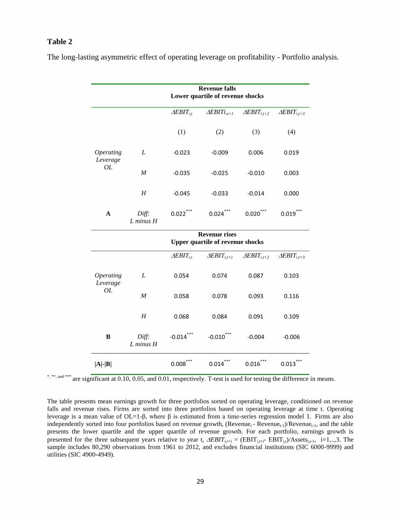
Testing the first hypothesis, results reported in Table 2 for revenue falls indicate that the

high-operating-leverage portfolio shows a slow earnings-adjustment process starting in the

concurrent year, -4.5%, which continues through the subsequent three years (-3.3%, -1.4%, and

0.0%, respectively). For the low-operating-leverage portfolio, we find an enduring earnings

response in the concurrent year and one year ahead (-2.3% and -0.9%, respectively), which

reverses to earnings growth in the second and third years ahead (+0.6% and +1.9%,

respectively). The findings indicate a monotonic earnings-adjustment process, which continues

through the three subsequent years beyond the contemporaneous response to the revenue falls.

That is, the earnings-adjustment process when revenue falls is enduring and lasts over three years

11

beyond the immediate response. As reported in row A of the table, the difference between the

earnings growth of the low- and high-operating-leverage firms is statistically significant in each

of the four years (p-value<.01). Overall, the results suggest that high operating leverage has a

negative long-lasting effect on future profitability when revenue falls. In contrast, firms with low

operating leverage have a significantly lower decrease in profitability over a shorter period.

When revenue rises, the earnings growth of firms in the high-operating-leverage portfolio is

higher than the earnings growth of firms in the low-operating-leverage portfolio. In the high-

operating-leverage portfolio, earnings grow by 6.8% in the year of the revenue shock, year t, and

by 8.4%, 9.1%, and 10.9% in years t+1, t+2, and t+3, respectively. For the low-operating-

leverage portfolio, earnings increase by 5.4%, 7.4%, 8.7%, and 10.3%, in years t to t+3,

respectively. As reported in row B, the difference between the earnings growth of the low- and

high-operating-leverage portfolios is statistically significant in years t and t+1 (p-value<.01).

Therefore, high operating leverage has a positive effect on future profitability one year after

revenue rises.

As a whole, we conclude that operating leverage has a positive (negative) long-lasting effect

on future profitability when revenue rises (falls), in line with the first hypothesis, and operating

leverage increases earnings volatility.

Next, we test our second hypothesis, that operating leverage has an asymmetric impact on

future earnings. The difference between the earnings growth of high- and low-operating-leverage

portfolios is presented in row A for revenue falls, and in row B for revenue rises. The difference

between these two effects is presented in the bottom row, marked |A|-|B|. We find that the

incremental impact of high operating leverage on earnings change when revenue falls on year tis

significantly greater than when revenue rises on year t, as well as in each of the three subsequent

years (p-value<.01 in each of the four years). For instance, the incremental impact of high

operating leverage over low operating leverage in the first subsequent year, t+1, is +1.4% (p-

value<0.01).6 That is, we observe that the difference in performance for the high-operating-

leverage group relative to the low-operating-leverage group (see bottom row) is much greater for

the negative revenue shocks (see row A) than for the positive shocks (see row B). This evidence 6 We also observe that in the low-operating-leverage portfolio of Table 2, 32.76% of observations have a revenues

decrease, while in the high-operating-leverage portfolio, 27.71% of observations have a revenue decrease. The

Wilcoxon test for the difference between the two proportions is 12.77 (p-value <.0001). Hence, the high-operating-

leverage portfolio experiences significantly more positive revenue shocks than the low-operating-leverage portfolio.

12

suggests operating leverage has an asymmetric impact on future earnings: future earnings

increase less when revenue rises than they decrease when revenue falls. Overall, our portfolio

analysis paints a clear picture in support of the second hypothesis.


To further test our two hypotheses, we also use a regression model with the following

specification:

ΔEBITi,t+k = α + β1 RevDeci,t + β2 OLi,t + β3 RevDeci,t OLi,t + β4 ΔEBITi,t-1 + β5 MVi,t-1

+ β6 BMi,t-1+εi,t, k= 0,1,2,3. (5)

We estimate equation (5) separately for changes in EBIT over each of four horizons, from

year t to year t+k, where k= 0,1, 2, 3. Thus, ΔEBITi,t+k is the accumulated change in earnings

before interest and taxes from year t to year t+k, where k goes from 0 to 3, deflated by total

assets at t-1. RevDeci,t is an indicator variable that equals 1 if revenue in year t was lower than

the revenue in year t-1. OLi,t is operating leverage defined as 1-βi,t, where βi,t is defined by

equation (1). ΔEBITi,t-1 is the change in earnings before interest and taxes from year t-2 to year t-

1, deflated by total assets at t-2. MV i, t-1 is the natural log of the market value of the firm at the

end of year t-1. B/M i, t-1 is the book value of equity divided by the market value of equity at the

end of year t-1. In addition, we include both year and industry fixed effects, using Fama and

French’s (1997) 12-industry classification. Finally, all significance levels are based on standard

errors that are clustered by firm and year.

The coefficients β2 and β3 are the focus of our tests. The association between operating

leverage and future earnings when revenue rises is captured by β2. The interactive term of

operating leverage multiplied by revenue fall, or more specifically, the coefficients β2+β3,

capture the association between operating leverage and future earnings when revenue falls.

Significant values for β2 (β2+β3) when k=1, 2, and 3 will support our first hypothesis that a

significant long-lasting association exists between operating leverage and future earnings.

According to the second hypothesis, operating leverage has a greater effect on future earnings

during revenue downswings than upswings, and the coefficient β3 is expected to be negative and

significant.

Our control variables are as follows: the change in EBIT from year t-2 to year t-1, ΔEBITi, t-1,

controls for the time-series properties of earnings that can affect future earnings. Market value,

13

MVi, t-1, and the book-to-market ratio, BMi, t-1, control for potential effects of risk and growth

(Fama and French, 1992).

Estimation results are reported in Table 3. Testing the first hypothesis, we find that operating

leverage has a long-lasting effect on future firm performance. For a positive revenue shock, the

contemporaneous (k=0) β2 is positive and significant (β2=0.029, t-statistic=9.56). The coefficient

β2 is also significant and positive for one year ahead (β2=0.022, t-statistic=3.68), and marginally

significant for two years ahead (β2=0.015, t-statistic=1.72). However, β2 is insignificant for three

years ahead (β2=0.014, t-statistic=1.20). In sum, when revenue rises, operating leverage affects

profitability growth two years ahead, and by the third year, the effect of operating leverage on

profitability fades.

When revenue falls, β2+β3 is significant and negative in year t (β2+β3=0.029-0.074=-0.045, t-

statistic= -7.69). Looking ahead, β2+β3 is significant and negative one year after the revenue

shock, at year t+1 (β2+β3 =0.022-0.066=-0.044, t-statistic= -4.04), two years ahead (β2+β3 =

0.015-0.059=-0.044, t-statistic= -3.03), and three years ahead (β2+β3 =0.014-0.054=-0.040, t-

statistic= -2.92). So when revenue falls, operating leverage has a long-lasting effect on

profitability, of at least three years.

In sum, we find that the association between operating leverage and future earnings is

significant two years ahead when revenue rises, and at least three years ahead when revenue

falls. These results suggest that operating leverage has a long-lasting effect on the earnings-

adjustment process, which continues beyond the year of the revenue shock, and is longer for

negative revenue shocks.

As for the control variables, ΔEBITi,t-1 is negative and significant, capturing the mean

reversion in operating performance. Similarly, both market value and market-to-book value are

significantly negative, indicating that larger and more mature firms have less volatility in their

operating performance.

The second hypothesis predicts that for high-operating-leverage firms, future earnings

increase less when revenue rises than they decrease when revenue falls. As reported in Table 3,

β3 is significant and negative in the year of the revenue shock, year t (β3=-0.074, t-statistic=-

12.02), β3 is significant and negative for earnings one year ahead, year t+1 (β3 =

-0.066, t-statistic=-6.46), for two years ahead (β3 = -0.059, t-statistic=-4.75), and for three years

14

ahead (β3 =-0.054, t-statistic=-4.90). That is, in the year of the revenue shock as well as in each

of the three subsequent years, β3 is negative and significant. The evidence suggests that operating

leverage enhances the asymmetric effect of revenue changes on profitability, consistent with the

second hypothesis.


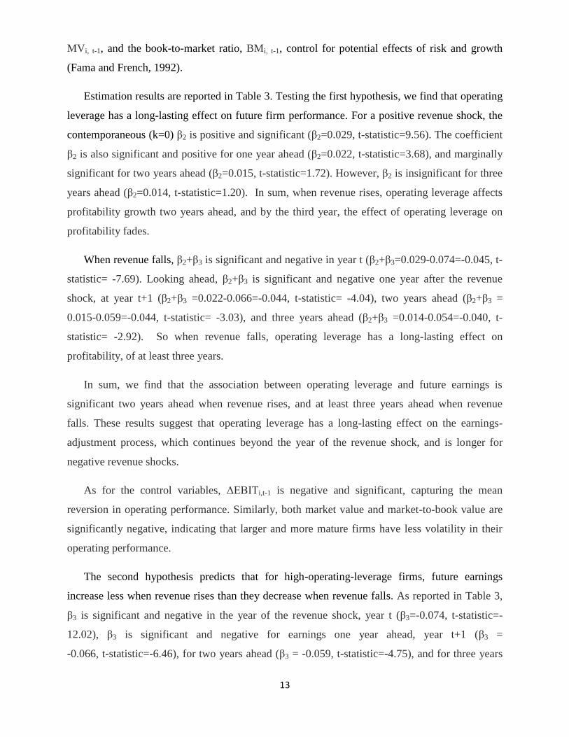
The final analysis in this section provides insight on the causes of the asymmetric effect that

operating leverage has on future profitability during negative and positive revenue shocks. As the

sticky cost literature shows, on average, costs increase more when revenue rises than they

decrease when revenue falls by an equivalent amount (Banker and Byzalov, 2014). This

phenomenon, on its own, would lead to operating-performance asymmetry as earnings increase

less when revenue rises than they decrease when revenue falls by an equivalent amount, as

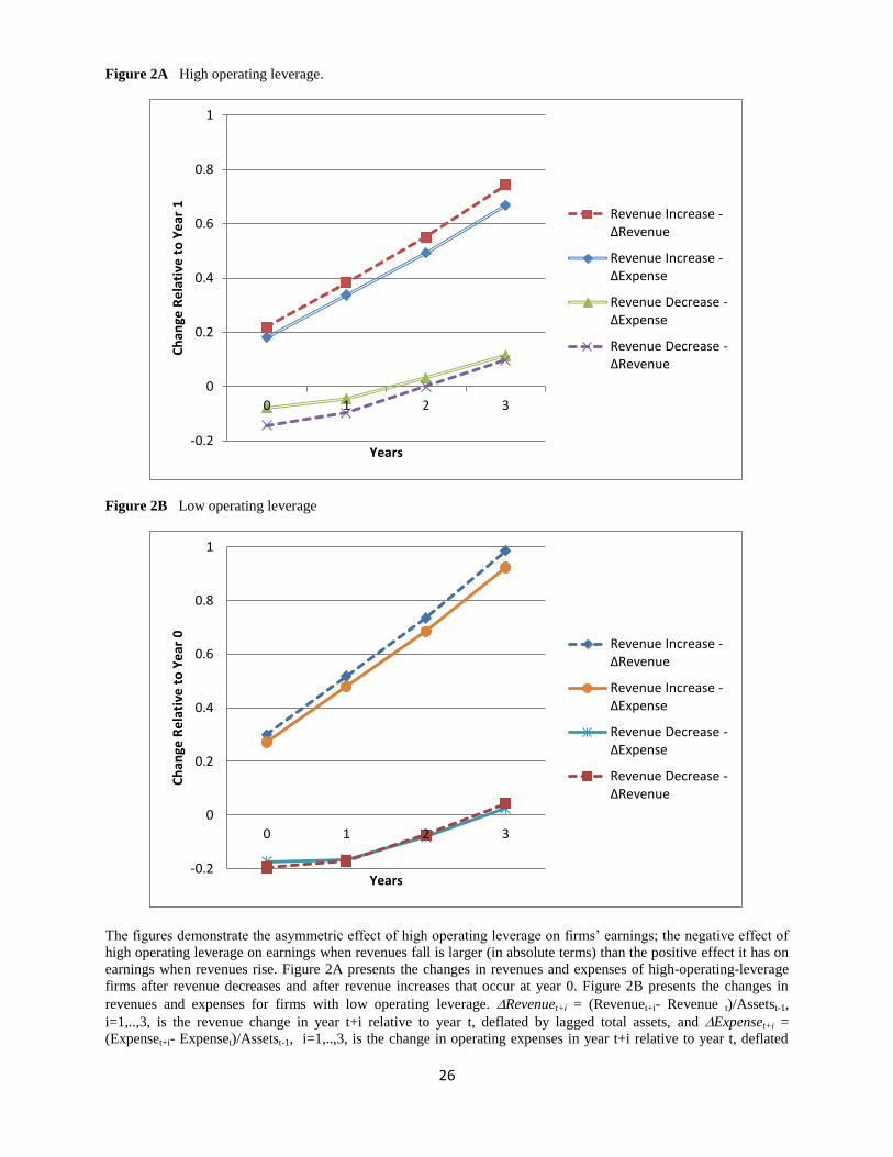
reported in Tables 2 and 3. In Figure 2, we separately analyze revenue and costs, and examine

their role in the performance asymmetry.

Figure 2A describes the expenses and revenues of firms with high operating leverage when

revenue rises and when revenue falls. The high-operating-leverage portfolio is defined as in

Table 2 and includes firms in the upper third of OL. When revenue falls, expenses decrease less

than revenue. The gap between revenues and expenses decreases in the years after the revenue

shock, indicating a slow adjustment process that takes about three years to stabilize. When

revenue rises at year t, both revenue and expenses increase linearly over the three subsequent

years. Thus, the asymmetry reported in Tables 2 and 3 for high-operating-leverage firms is

driven primarily by slow adjustment of expenses in response to revenue falls.

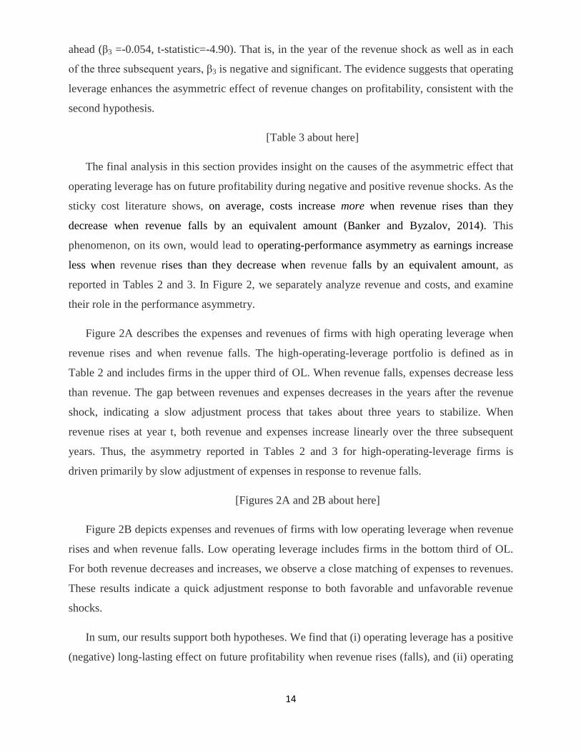
[Figures 2A and 2B about here]

Figure 2B depicts expenses and revenues of firms with low operating leverage when revenue

rises and when revenue falls. Low operating leverage includes firms in the bottom third of OL.

For both revenue decreases and increases, we observe a close matching of expenses to revenues.

These results indicate a quick adjustment response to both favorable and unfavorable revenue

shocks.

In sum, our results support both hypotheses. We find that (i) operating leverage has a positive

(negative) long-lasting effect on future profitability when revenue rises (falls), and (ii) operating

15

leverage has an asymmetric impact on future earnings: future earnings increase less when

revenue rises than they decrease when revenue falls.

5. Contextual Analyses

We perform three contextual analyses to provide support to our main results on the long-

lasting impact of operating leverage on future earnings.

5.1 Comparative Industry Analysis

We compare the effect of the impact of operating leverage on future earnings in two

industries: retailers, which is the industry with the lowest operating leverage in our sample,

OL=0.004, with pharmaceuticals, which is the industry with the highest operating leverage in our

sample, OL=0.106. Industry definition is based on Fama and French’s (1997) 48-industry

classification.

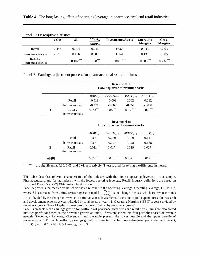
Results reported in Panel A of Table 4 indicate a meaningful difference in the attributes of

the two industries. First, the gross and operating margins of retailers are 30.3% and 4.3%,

respectively. By contrast, the gross and operating margins of pharmaceutical firms are 58.5% and

13.1%, respectively. The difference in gross and operating margins of the two industries is

highly significant (p-value<0.01). The significant difference is consistent with a lower operating

leverage in the retailing industry than in the pharmaceutical industry.

Second, we compare the cost response to demand shocks. Specifically, ∆𝐶𝑜𝑠𝑡𝑖𝑡

∆𝑅𝑒𝑣𝑖𝑡 is the change

in costs, which are revenue minus EBIT, divided by the change in revenue of firm i at year t. We

compute this variable only when costs and revenue change in the same direction.7 The findings

show a significant gap in the level of cost response between the two industries: 0.946 for retailers

and 0.808 for pharmaceutical firms. That is, retailers adjust more costs than pharmaceutical firms

in response to an equivalent change in revenue. Therefore, cost variability in the retailing

industry is higher than in the pharmaceutical industry. Again, this result is in line with lower

operating leverage in the retailing industry than in the pharmaceutical industry.

7 Costs response is in an opposite direction to the revenue shock in about 15% of our sample observations (costs rise

when revenue falls or vice versa). See Weiss (2010) and Banker and Byzalov (2014) for discussions of this issue.

16

Results reported in Panel B for revenue falls indicate that pharmaceutical firms have a slow

earnings-adjustment process, which starts in the year of the revenue fall and continues in the

subsequent three years (-7.4%, -6.9%, -5.4%, and -3.4%, respectively). The earnings change of

retail firms is -1.9% in the year of the revenue fall, and -0.9%, +0.2%, and +1.2% in the three

subsequent years, respectively. The results demonstrate that pharmaceutical firms, which are

characterized by high operating leverage, do worse than retail firms in adjusting to revenue falls.

Specifically, retailers’ earnings decline less than the earnings of pharmaceutical firms in the year

of the revenue shock and in the following year, and retailers’ earnings bounce back and grow in

the second and third years after the revenue shock. Overall, the results for revenue falls suggest

that pharmaceutical firms characterized by high operating leverage have significantly more

negative long-lasting earnings changes in the three subsequent years compared with retail firms

with low operating leverage (p-value<0.01 in all the years; see row A in Panel B).

Results reported for revenue rises indicate the pharmaceutical firms with high operating

leverage show an ongoing improvement in earnings starting in the concurrent year as well as in

the subsequent three years (p-value<0.01 in all the years; see row B in Panel B). Again, the

earnings-adjustment process when revenue rises is enduring and lasts over three years beyond

the contemporaneous response. Testing the difference between the industries when revenue rises,

results reported in row B show that pharmaceutical firms make greater adjustments to revenue

increases in the concurrent year and in all three years ahead (p-value<0.01, 0.05, 0.10, and 0.05

on years t, t+1, t+2, and t+3 respectively). That is, pharmaceutical firms characterized by high

operating leverage have a positive effect on future profitability when revenue rises, which

continues three years ahead. As a whole, the comparative industry analysis illustrates the positive

(negative) long-lasting effect of operating leverage on future profitability when revenue rises

(falls), and reconfirms the first hypothesis.

Demonstrating the asymmetric effect, the incremental impact of high operating leverage in

pharmaceutical firms on future earnings growth over retail firms is presented in row A for

revenue decreases, and in row B for revenue increases. As in Table 2, the difference between

these two rows is presented in the bottom row, marked |A|-|B|. The evidence suggests that high

operating leverage in pharmaceutical firms increases the asymmetric impact on future earnings

relative to retailers with low operating leverage: future earnings increase less when revenue rises

than they decrease when revenue falls. This result reconfirms the second hypothesis.

17


5.2 Operating Leverage and Macro Conditions

As reported earlier, high operating leverage has a negative long-lasting effect on firms’

profitability when revenue rises. If negative revenue shocks are infrequent, firms might choose

high operating leverage to benefit from the more frequent positive shocks or expansion in the

economy. As reported in Panel A of Table 1, firms’ revenue increase 71.5% of the time, and

decrease only 28.5% of the time in our sample. Thus, managers might choose high operating

leverage to benefit from the higher frequency of revenue increases.

To further investigate this issue, we separate the sample years to low, medium, and high GDP

growth years (GDP data are taken from the NBER). We report our results in Table 5. Looking at

the low GDP growth years, we observe that the contemporaneous performance of the low-

operating-leverage group is significantly higher than the high-operating-leverage group. Whereas

the low-operating-leverage group has an increase of 0.7% in its operating performance, the high-

operating-leverage group exhibits a decrease of -0.2% in its performance, and the difference is

significant at the 1% level. That is, firms with low operating leverage outperform those with

high operating leverage in low GDP periods. The difference in performance persists for one year

and two years ahead. However, the three-year-ahead earnings growth of the low- and high-

operating-leverage portfolios are insignificantly different from each other. Overall, low operating

leverage is advantageous in low GDP growth periods. For the medium GDP growth period, we

observe no significant difference in performance across all operating-leverage portfolios.

Results for the high GDP growth years indicate that future earnings grow more for the high-

operating-leverage group than for low- or medium-operating-leverage groups. Specifically, for

the one-, two-, and three-year-ahead performance for the low-operating-leverage group, the

increase in performance is 3.0%, 4.0%, and 5.1%, respectively. For the one-, two-, and three-

year-ahead performance for the high-operating-leverage group, the increase in performance is

3.7%, 5.2%, and 7.6%, respectively. All differences are significant at the 1% level. That is, the

high-operating-leverage group outperforms both the low- and medium-operating-leverage groups

in each of the one-, two-, and three-year-ahead portfolios. Taken together, our results indicate the

benefits from high operating leverage are pronounced in periods of high economic expansion.


18

5.3 Two Consecutive Negative versus Positive Revenue Shocks

To gain further insights on the impact of operating leverage on future earnings, conditional

on unfolding demand, we examine the phenomena in hand in periods following two consecutive

increases or decreases in revenue (rather than a single revenue shock examined earlier).

Specifically, we also sort firms into two portfolios based on their revenue growth. Two

consecutive revenue decreases are firms with revenue decreases in both years t and t+1. Two

consecutive revenue increases are firms with revenue increases in both years t and t+1. In each of

the two portfolios,8 we also sort firms into three portfolios based on operating leverage at time t.

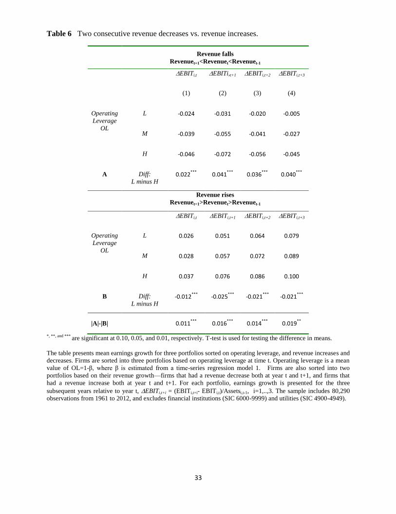
Results reported in Table 6 for two consecutive revenue decreases indicate a monotonic

relationship between the operating-leverage portfolio and firm performance in the

contemporaneous and one-, two-, and three-year-ahead portfolios. Notably, earnings decline

significantly more for high-operating-leverage firms than for low-operating-leverage firms in the

contemporaneous and one-, two-, and three-year-ahead portfolios. For two negative consecutive

revenue shocks, the findings reconfirm the earlier results for the single revenue shock reported in

Table 2. By contrast, for two consecutive revenue increases, earnings increase significantly

more for high-operating-leverage firms than for low-operating-leverage firms in the

contemporaneous and one-, two-, and three-year-ahead portfolios. For two positive consecutive

revenue shocks, the findings indicate a long-lasting effect over three subsequent years, which is

longer than the effect reported in Table 2 for the single demand shock. Overall, consistent with

the first hypothesis, the findings indicate a long-lasting impact of operating leverage on future

earnings growth in three subsequent years.

Testing the second hypothesis, the under-performance of firms with high operating leverage

over firms with low operating leverage on the downside significantly exceeds the over-

performance of firms with high operating leverage over firms with low operating leverage on the

upside (see results reported in the bottom row in Table 6). That is, the results show a clear

asymmetry between the impact of operating leverage when revenues fall in two consecutive

periods and the impact of operating leverage when revenues rise in two consecutive periods.

8 The portfolio with two consecutive revenue increases has 41,254 observations, and the portfolio with two

consecutive revenue decreases has 11,242 observations.

19

Taken as a whole, the findings in the context of two consecutive revenue shocks indicate (i)

operating leverage has a positive (negative) long-lasting effect on future profitability, and (ii)

operating leverage has an asymmetric impact on future earnings.


6. COSTS AND BENEFITS OF OPERATING LEVERAGE

Our results indicate the outcome of a negative revenue shock is more severe than the benefits

from a positive revenue shock for high-operating-leverage firms. This result raises an interesting

question of why risk-averse managers adopt a high operating leverage. The remainder of our

study suggests why some managers adopt a high operating leverage and others do not.

6.1 Operating Leverage and Financial Leverage

As documented in our main findings, firms with higher operating leverage experience low

operating performance when revenue falls. An adverse shock in revenues could force firms to

forgo profitable projects, violate debt covenants, or even default and go into potentially costly

financial distress. Hence, we expect that high fixed-cost firms will choose more conservative

financial policies. Van Horne (1977) suggests that high fixed-cost firms choose a lower leverage

ratio as a means for financial flexibility. Kahl et al. (2013) report a tradeoff between operating

leverage and financial leverage.

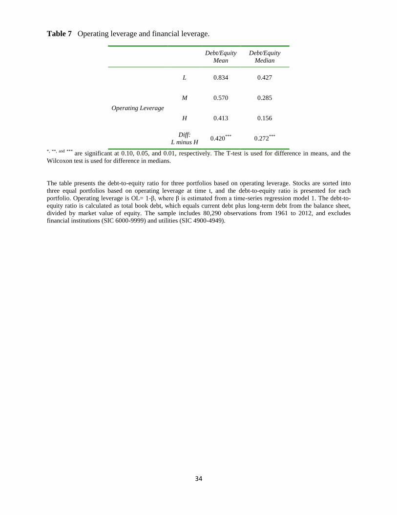
To examine Van Horne’s claim, Table 7 presents mean and median values of debt-to-equity

ratios for three equal portfolios classified by operating leverage. The debt-to-equity ratio is

calculated as total book debt, which is the sum of current debt and long-term debt from the

balance sheet, divided by market value of equity. As expected, we find a monotonic relationship

between the debt-to-equity ratio and operating leverage for both the mean and median.

Specifically, the mean debt-to-equity ratio decreases from 0.834 in the low-operating-leverage

group, to 0.570 in the medium-operating-leverage group, to 0.413 in the high-operating-leverage

group.

Consistent with Van Horne’s claim, we find a tradeoff between financial leverage and

operating leverage. The results suggest that firms with high financial leverage manage their real

resources to achieve low operating leverage, or vice versa. An alternative explanation for the

20

tradeoff is that the high earnings volatility induced by high operating leverage reduces firms’

debt capacity and leads them to lower their financial leverage.


6.2 Operating Leverage and Management Compensation

Lastly, assuming managers are risk averse, high operating leverage exposes them to

additional risk. Operating leverage increases earnings volatility, and firms are expected to

compensate the managers for this precariousness. Without proper incentives, managers will

choose a suboptimal level of operating leverage for the firm. We test the association between

operating leverage and executive equity-based compensation using a portfolio analysis.

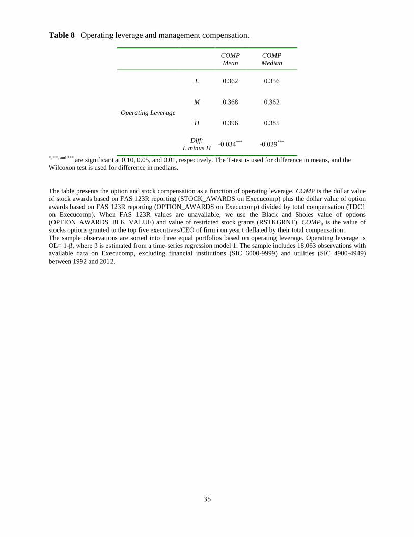
Table 8 presents mean and median values of executive compensation for three equal

portfolios sorted by operating leverage. Executive compensation, COMP, is the dollar value of

stock awards based on FAS 123R reporting (STOCK_AWARDS on Execucomp) plus the dollar

value of option awards based on FAS 123R reporting (OPTION_AWARDS on Execucomp)

divided by total compensation (TDC1 on Execucomp). When FAS 123R values are unavailable,

we use the Black and Sholes value of options (OPTION_AWARDS_BLK_VALUE) and value

of restricted stock grants (RSTKGRNT).

Results reported in Table 8 indicate a monotonic relationship between COMP and operating

leverage. Specifically, the mean COMP increases from 0.362 for the low-operating-leverage

group, to 0.368 for the medium-operating-leverage group, to 0.396 for the high-operating-

leverage group. The median ratio follows a similar pattern.9

The results suggest that high-operating-leverage is associated with greater equity-based

compensation. That is, executives are protected on the downside from the unfavorable revenue

shocks and benefit from the upside of greater earnings volatility. As such, options provide a

better incentive alignment for the extra risk that high operating leverage imposes on executives.

Taken together, our results indicate that boards understand the implications of operating leverage

and to a reasonable extent, efficiently align the incentives of their executives with the operating

environment of the firm.


9 Further checking the robustness of the evidence, we find that untabulated results from estimating a regression

model with additional control variables (size, book-to-market ratio, and sales volatility) reconfirm the findings.

21

7. Summary

This study examines the effect of operating leverage on firms’ future earnings. We predict

and find that operating leverage has a long-lasting impact on future firm performance. In line

with expectations, we show that high operating leverage increases earnings volatility due to a

slower cost-adjustment process for high-operating-leverage firms. More importantly, we find that

operating leverage has an asymmetric effect on future operating performance. Specifically,

operating leverage has a larger effect on earnings when revenue falls than when revenue rises.

Further investigation reveals that a slower cost-adjustment process on the downside primarily

drives the asymmetric effect. Turning to the costs and benefits of high operating leverage, we

find effects on firms’ capital structure and on executive equity-based compensation. Overall, our

study is an important addition to two streams of literatures: operating leverage and cost behavior.

22

Reference

Anderson, M., Banker, R., Huang, R., Janakiraman, S. 2007. Cost behavior and fundamental

analysis of SG&A costs. J. of Account. Audit. and Finance. 22 (1), 1-28.

Anderson, M., Banker, R., Janakiraman, S. 2003. Are selling, general and administrative costs

"sticky?” J. of Account. Res. 41, 47-63.

Balakrishnan, R., Gruca, T. S. 2008. Cost stickiness and core competency: A note.

Contemp. Account. Res. 25 (4), 993–1006.

Balakrishnan, R., Labro, E., Soderstrom, N. 2013. Cost structure and sticky costs. J of

Management Acct Res. Forthcoming.

Balakrishnan, R., Petersen, M., Soderstrom, N. 2004. Does capacity utilization affect the

“stickiness” of cost? J. of Account. Audit. and Finance. 19, 283-299.

Balakrishnan, R., Sivaramakrishnan, K., Sprinkle, G., 2013. Managerial Accounting. Wiley,

New York.

Banker, R. D., Byzalov, D., Ciftci, M., Mashruwala, M. 2013. The moderating effect of prior

revenues changes on asymmetric cost behavior. J of Management Acct Res.

Forthcoming..

Banker, R. D., Byzalov, D. 2014. Asymmetric cost behavior. J of Management Acct Res.

Forthcoming.

Banker, R. D., D. Byzalov, and L. Chen. 2013. Employment protection legislation, adjustment

costs and cross-country differences in cost behavior. J of Account and Econ. 55(1): 111–

127.

.Banker, R.D., Byzalov, D., Plehn-Dujowich, J. 2014. Sticky cost behavior: Theory and

evidence. The Account. Rev. Forthcoming.

Banker, R.D., Chen, L. 2006. Predicting earnings using a model of cost variability and cost

stickiness. The Account. Rev. 78, 285-307.

Banker, R. D., Potter, G., Schroeder, R. G. 1995. An empirical analysis of manufacturing

overhead cost drivers. J. of Account. and Econ. 19, 115–37.

Cannon, J.N. 2014. Determinants of "sticky costs": An analysis of cost behavior using United

States air transportation industry data. The Account. Rev. Forthcoming.

Chen, C. X., Lu, H., Sougiannis, T. 2012. The agency problem, corporate governance, and the

asymmetrical behavior of selling, general, and administrative costs. Contemp. Account.

Res. 29, 252–282.

23

Dechow, P., Kothari, S., Watts, R. 1998. The relation between earnings and cash flows. J. of

Account. and Econ. 25, 133-168.

Dierynck, B., Landsman, W., Renders, A. 2012. Do managerial incentives drive cost behavior?

Evidence about the role of the zero earnings benchmark for labor cost behavior in

Belgian private firms. The Account. Rev. 87(4), 1219-1246.

Fama, E. F., French, K. R. 1992. The cross-section of expected stock returns. J.

of Finance. 47, 427-465.

Fama, E. F., French, K. R., 1997. Industry costs of equity. J. of Financial Econ.

43, 153-193.

Garrison, R. H., Noreen, E. W., Brewer, P. C. 2012. Managerial Accounting, 14th

ed. McGraw

Hill, New York.

Holzhacker, M., Krishnan, R., Mahlendorf, M. 2014. The impact of changes in regulation on cost

behavior. Contemp. Account. Res. Forthcoming.

Horngren, C. T., Sundem, G. L., Schwartzberg, J. O., Burgstahler, D. 2013. Introduction to

Management Accounting, 16th

ed. Pearson, Upper Saddle River, NJ.

Kahl, M., Null, J., Nilsson, M. 2013. Operating leverage and corporate financial policies.

Working paper, University of Colorado at Boulder.

Kallapur, S., Eldenburg, L. 2005. Uncertainty, real options, and cost behavior: Evidence from

Washington State hospitals. J. of Account. Res. 43 (5), 735-752.

Kama, I., Weiss, D. 2013. Do earnings targets and managerial incentives affect sticky costs? J. of

Account. Res. 51 (1), 201–224.

Lev, B. 1974. On the association between operating leverage and risk. J. of Financial and Quant.

Anal. 9, 627-641.

Lanen, W. N., Anderson, S., Maher, M. 2013. Fundamentals of Cost Accounting. McGraw Hill

Irwin, New York.

Mandelker, G.N., Rhee, S.G., 1984. The impact of the degrees of operating and financial

leverage on systematic risk of common stock. J. of Financial and Quant. Anal. 19, 45-57.

Noreen, E., and N. Soderstrom. 1994. Are overhead costs strictly proportional to activity?

Evidence from hospital service departments. J. of Account. and Econ. 17, 255–278.

Noreen, E., Soderstrom, N. 1997. The accuracy of proportional cost models: Evidence from

hospital service departments. Rev. of Account. Stud. 2, 89–114.

Novy-Marx, R. 2010. Operating leverage. Rev. of Finance. 15, 103-134.

24

Shust, E., Weiss, D. Discussion of asymmetric cost behavior: Cash flow versus expenses. J. of

Manag. Account. Res.. Forthcoming.

Van Horne, J. C. 1977. Financial Management and Policy. Prentice-Hall, Englewood Cliffs, NJ.

Weiss, D. 2010. Cost behavior and analysts’ earnings forecasts. The Account. Rev. 85,1441–

1474.

25

Figure 1 Timeline for operating-leverage estimation.

t-8… …t-1 t t+1 t+3

Estimation of Operating

Leverage (OL)

Testing the Effect of OL on

Earnings Growth

t+2

26

Figure 2A High operating leverage.

Figure 2B Low operating leverage

The figures demonstrate the asymmetric effect of high operating leverage on firms’ earnings; the negative effect of

high operating leverage on earnings when revenues fall is larger (in absolute terms) than the positive effect it has on

earnings when revenues rise. Figure 2A presents the changes in revenues and expenses of high-operating-leverage

firms after revenue decreases and after revenue increases that occur at year 0. Figure 2B presents the changes in

revenues and expenses for firms with low operating leverage. Revenuet+i = (Revenuet+i- Revenue t)/Assetst-1,

i=1,..,3, is the revenue change in year t+i relative to year t, deflated by lagged total assets, and Expenset+i =

(Expenset+i- Expenset)/Assetst-1, i=1,..,3, is the change in operating expenses in year t+i relative to year t, deflated

-0.2

0

0.2

0.4

0.6

0.8

1

0 1 2 3

Ch

ange

Re

lati

ve t

o Y

ear

1

Years

Revenue Increase - ∆Revenue

Revenue Increase -∆Expense

Revenue Decrease - ∆Expense

Revenue Decrease - ∆Revenue

-0.2

0

0.2

0.4

0.6

0.8

1

0 1 2 3

Ch

ange

Re

lati

ve t

o Y

ear

0

Years

Revenue Increase - ∆Revenue

Revenue Increase - ∆Expense

Revenue Decrease - ∆Expense

Revenue Decrease - ∆Revenue

27

by lagged total assets, and operating expenses are revenue minus earnings before interest and taxes. In each year,

stocks are sorted into three portfolios based on operating leverage, and the figures present the results for firms in the

high- and low-operating-leverage portfolios. Operating leverage is OL=1-β, where β is estimated from a time-series

regression presented in model 1.

28

Table 1 Descriptive statistics.

Panel A: Descriptive statistics

Lower

Upper

Variable N Mean Quartile Median Quartile Std Dev Minimum Maximum

OLi,t (=1- βi,t) 80,290 0.076 -0.017 0.030 0.119 0.190 -0.452 1.123

EBITi,t 80,290 0.010 -0.020 0.012 0.042 0.082 -0.493 0.440

EBITi,t+1 74,295 0.022 -0.027 0.020 0.070 0.120 -0.656 0.609

EBITi,t+2 68,833 0.036 -0.029 0.028 0.094 0.148 -0.774 0.793

EBITi,t+3 63,764 0.051 -0.030 0.037 0.116 0.175 -0.718 1.109

RevDeci,t 80,290 0.286 0 0 1 0.452 0 1

EBITi,t-1 80,290 0.011 -0.018 0.012 0.040 0.074 -0.347 0.453

MVi,t 80,290 5.162 3.513 4.994 6.635 2.144 0.000 13.348

B/Mi,t 80,290 0.883 0.402 0.674 1.112 0.750 0.000 8.133

Panel B: Pearson correlations

EBITi,t EBITi,t+1 EBITi,t+2 EBITi,t+3 RevDeci,t EBITi,t-1 MVi,t B/Mi,t

OLi,t -0.01***

-0.02***

-0.02***

-0.01***

0.07***

0.03***

-0.1***

-0.08***

EBITi,t 0.63***

0.44***

0.36***

-0.36***

-0.04***

0.01***

-0.04***

EBITi,t+1

0.72***

0.54***

-0.24***

-0.11***

0.00 -0.02***

EBITi,t+2

0.76***

-0.18***

-0.11***

0.01* -0.02

***

EBITi,t+3

-0.16***

-0.08***

0.02***

-0.03***

RevDeci,t

-0.11***

-0.14***

0.16***

EBITi,t-1

0.07***

-0.14***

MVi,t

-0.51 *, **, and ***

are significant at 0.10, 0.05, and 0.01, respectively.

Operating leverage, OLi,t, is 1-βi,t, where βi,t is estimated from a time-series regression model 1. EBITi,t+i is the

change in earnings before interest and taxes from year t to year t+i, deflated by total assets, at t-1, i=1,..,3. RevDec i,t

is an indicator variable that equals 1 if revenue in year t was lower than the revenue in year t. EBITi,t-1 is the

change in earnings before interest and taxes from year t-2 to year t-1, deflated by lagged total assets. MVi,t is the

natural log of the market value of the firm at the end of year t. B/Mi,t is the book value of equity divided by the

market value of equity at the end of year t. The sample includes 80,290 observations from 1961 to 2012. It excludes

financial institutions (SIC 6000-9999) and utilities (SIC 4900-4949), and firms with total assets lower than $10

million, and firms with negative book value of equity.

29

Table 2

The long-lasting asymmetric effect of operating leverage on profitability - Portfolio analysis.

Revenue falls

Lower quartile of revenue shocks

EBITi,t EBITi,t+1 EBITi,t+2 EBITi,t+3

(1) (2) (3) (4)

Operating

Leverage

OL

L -0.023 -0.009 0.006 0.019

M -0.035 -0.025 -0.010 0.003

H -0.045 -0.033 -0.014 0.000

A Diff:

L minus H 0.022

*** 0.024

*** 0.020

*** 0.019

***

Revenue rises

Upper quartile of revenue shocks


Operating

Leverage

OL

L 0.054 0.074 0.087 0.103

M 0.058 0.078 0.093 0.116

H 0.068 0.084 0.091 0.109

B Diff:

L minus H -0.014

*** -0.010

*** -0.004 -0.006

|A|-|B| 0.008***

0.014***

0.016***

0.013***

*, **, and *** are significant at 0.10, 0.05, and 0.01, respectively. T-test is used for testing the difference in means.

The table presents mean earnings growth for three portfolios sorted on operating leverage, conditioned on revenue

falls and revenue rises. Firms are sorted into three portfolios based on operating leverage at time t. Operating

leverage is a mean value of OL=1-β, where β is estimated from a time-series regression model 1. Firms are also

independently sorted into four portfolios based on revenue growth, (Revenuet - Revenuet-1)/Revenuet-1, and the table

presents the lower quartile and the upper quartile of revenue growth. For each portfolio, earnings growth is

presented for the three subsequent years relative to year t, EBITi,t+i = (EBITi,t+i- EBITi,t)/Assetsi,t-1, i=1,..,3. The

sample includes 80,290 observations from 1961 to 2012, and excludes financial institutions (SIC 6000-9999) and

utilities (SIC 4900-4949).

30

Table 3 The long-lasting effect of operating leverage on profitability - Regression analysis.

ΔEBITi,t+k = α + β1 RevDeci,t + β2 OLi,t + β3 RevDeci,t OLi,t + β4 ΔEBITi,t-1 + β5 MVi,t-1

+ β6 BMi,t-1+εi,t, k= 0,1,2,3 (5)

Dependent Variables

Independent Variables EBITt EBITt+1 EBITt+2 EBITt+3

RevDect -0.061 -0.062 -0.058 -0.059 (-34.29)

*** (-28.68)

*** (-21.66)

*** (-21.17)

***

OLt 0.029 0.022 0.015 0.014 (9.56)

*** (3.68)

*** (1.72)

* (1.20)

RevDect OLt -0.074 -0.066 -0.059 -0.054 (-12.02)

*** (-6.46)

*** (-4.75)

*** (-4.90)

***

EBITt-1 -0.082 -0.211 -0.258 -0.249 (-4.27)

*** (-6.84)

*** (-8.94)

*** (-8.66)

***

MVt-1 -0.002 -0.001 -0.001 -0.001 (-5.71)

*** (-2.74)

*** (-1.37) (-0.88)

B/Mt-1 -0.002 -0.004 -0.008 -0.013 (-1.60) (-1.93)

* (-3.28)

*** (-3.99)

***

Observations 80,290 74,295 68,833 63,764

Adjusted R2 18.12% 13.65% 11.55% 10.70%

OLt + RevDect OLt -0.045 -0.044 -0.044 -0.040

(-7.69)***

(-4.04)***

(-3.03)***

(-2.92)***

*, **, and ***

are significant at 0.10, 0.05, and 0.01, respectively. Values in parentheses are t-statistics.

This table estimates the relation between operating leverage and future earnings growth. Operating leverage, OL, is

1-β, where β is estimated from a time-series regression model 1. EBITi,t+i is the change in earnings before interest

and taxes from year t to year t+i, deflated by total assets, at t-1, i=1,..,3. RevDec i,t is an indicator variable that

equals 1 if revenue in year t was lower than revenue in year t-1. EBITt-1 is the change in earnings before interest

and taxes from year t-2 to year t-1, deflated by lagged total assets. MVi,t is the natural log of the market value of the

firm at the end of year t. B/Mi,t is the book value of equity divided by the market value of equity at the end of year t.

The sample includes 80,155 observations from 1961 to 2012, and excludes financial institutions (SIC 6000-9999)

and utilities (SIC 4900-4949). Regression is estimated with industry (12-industry classification from Fama and

French (1997)) and year fixed effects. Errors are clustered on year and firm.

31

Table 4 The long-lasting effect of operating leverage in pharmaceutical and retail industries.

Panel A: Descriptive statistics # Obs OL ∆𝑪𝒐𝒔𝒕𝒊𝒕

∆𝑹𝒆𝒗𝒊𝒕

Investments/Assets Operating

Margins

Gross

Margins

Retail 6,498 0.004 0.946 0.068 0.043 0.303

Pharmaceuticals 2,596 0.106 0.808 0.144 0.131 0.585

Retail -

Pharmaceuticals -0.102

*** 0.138

*** -0.076

*** -0.088

*** -0.282

***

Panel B: Earnings-adjustment process for pharmaceutical vs. retail firms

Revenue falls

Lower quartile of revenue shocks


Retail -0.019 -0.009 0.002 0.012

Pharmaceuticals -0.074 -0.069 -0.054 -0.034

A Retail -

Pharmaceuticals

0.054***

0.060***

0.056***

0.046***

Revenue rises

Upper quartile of revenue shocks


Retail 0.051 0.079 0.109 0.141

Pharmaceuticals 0.071 0.097 0.128 0.168

B Retail -

Pharmaceuticals

-0.021***

-0.017**

-0.019*

-0.027**

|A|-|B| 0.033***

0.043***

0.037***

0.019***


This table describes relevant characteristics of the industry with the highest operating leverage in our sample,

Pharmaceuticals, and for the industry with the lowest operating leverage, Retail. Industry definitions are based on

Fama and French’s (1997) 48-industry classification.

Panel A presents the median values of variables relevant to the operating leverage. Operating leverage, OL, is 1-β,

where β is estimated from a time-series regression model 1. ∆𝐶𝑜𝑠𝑡𝑖𝑡

∆𝑅𝑒𝑣𝑖𝑡 is the change in costs, which are revenue minus

EBIT, divided by the change in revenue of firm i at year t. Investments/Assets are capital expenditures plus research

and development expense at year t divided by total assets at year t-1. Operating Margins is EBIT at year t divided by

revenue at year t. Gross Margins is gross profit at year t divided by revenue at year t-1.

Panel B presents mean earnings growth for portfolios of pharmaceutical firms and retail firms. Firms are also sorted

into two portfolios based on their revenue growth at time t—firms are sorted into four portfolios based on revenue

growth, (Revenuet - Revenuet-1)/Revenuet-1, and the table presents the lower quartile and the upper quartile of

revenue growth. For each portfolio, earnings growth is presented for the three subsequent years relative to year t,

EBITi,t+i = (EBITi,t+i- EBITi,t)/Assetsi,t-1, i=1,..,3.

32

Table 5 The effect of operating leverage on firms’ performance in good and bad economies.

Operating Leverage EBITi,t EBITi,t+1 EBITi,t+2 EBITi,t+3

Low GDP

growth

years

L 0.007 0.024 0.041 0.059

M 0.001 0.014 0.032 0.053

H -0.002 0.011 0.034 0.060

Diff: L minus H 0.009***

0.013***

0.007* 0.000

Medium

GDP

growth

years

L 0.012 0.025 0.037 0.045

M 0.011 0.021 0.030 0.037

H 0.013 0.021 0.034 0.042

Diff: L minus H -0.001 0.004 0.004 0.003

High

GDP

growth

years

L 0.018 0.030 0.040 0.051

M 0.018 0.030 0.040 0.058

H 0.021 0.037 0.052 0.076

Diff: L minus H -0.003**

-0.007***

-0.012***

-0.025***

*, **, and ***

are significant at 0.10, 0.05, and 0.01, respectively. T-test is used for testing the difference in means.

The table presents mean earnings growth based on operating leverage and GDP growth. In each year t, firms are

sorted into three portfolios on operating leverage. Operating leverage is a mean value of OL= 1-β, where β is

estimated from a time-series regression model 1. The sample years are sorted into three portfolios based on the US

GDP growth at year t, and three operating-leverage portfolios are presented for the low, medium, and high GDP

growth years. For each portfolio, earnings growth relative to year t is presented for three subsequent years, EBITi,t+i

= (EBITi,t+i- EBITi,t)/Assetsi,t-1, i=1,..,3. The sample includes 46,728 annual earnings announcements with December

fiscal year end between 1961 and 2012, and excludes financial institutions (SIC 6000-9999) and utilities (SIC 4900-

4949).

33

Table 6 Two consecutive revenue decreases vs. revenue increases.

Revenue falls

Revenuet+1<Revenuet<Revenuet-1


(1) (2) (3) (4)

Operating

Leverage

OL

L -0.024 -0.031 -0.020 -0.005

M -0.039 -0.055 -0.041 -0.027

H -0.046 -0.072 -0.056 -0.045

A Diff:

L minus H 0.022

*** 0.041

*** 0.036

*** 0.040

***

Revenue rises

Revenuet+1>Revenuet>Revenuet-1


Operating

Leverage

OL

L 0.026 0.051 0.064 0.079

M 0.028 0.057 0.072 0.089

H 0.037 0.076 0.086 0.100

B Diff:

L minus H -0.012

*** -0.025

*** -0.021

*** -0.021

***

|A|-|B| 0.011***

0.016***

0.014***

0.019**


The table presents mean earnings growth for three portfolios sorted on operating leverage, and revenue increases and

decreases. Firms are sorted into three portfolios based on operating leverage at time t. Operating leverage is a mean

value of OL=1-β, where β is estimated from a time-series regression model 1. Firms are also sorted into two

portfolios based on their revenue growth—firms that had a revenue decrease both at year t and t+1, and firms that

had a revenue increase both at year t and t+1. For each portfolio, earnings growth is presented for the three

subsequent years relative to year t, EBITi,t+i = (EBITi,t+i- EBITi,t)/Assetsi,t-1, i=1,..,3. The sample includes 80,290

observations from 1961 to 2012, and excludes financial institutions (SIC 6000-9999) and utilities (SIC 4900-4949).

34

Table 7 Operating leverage and financial leverage.

Debt/Equity

Mean

Debt/Equity

Median

Operating Leverage

L 0.834 0.427

M 0.570 0.285

H 0.413 0.156

Diff:

L minus H 0.420

*** 0.272

***

*, **, and *** are significant at 0.10, 0.05, and 0.01, respectively. The T-test is used for difference in means, and the

Wilcoxon test is used for difference in medians.

The table presents the debt-to-equity ratio for three portfolios based on operating leverage. Stocks are sorted into

three equal portfolios based on operating leverage at time t, and the debt-to-equity ratio is presented for each

portfolio. Operating leverage is OL= 1-β, where β is estimated from a time-series regression model 1. The debt-to-

equity ratio is calculated as total book debt, which equals current debt plus long-term debt from the balance sheet,

divided by market value of equity. The sample includes 80,290 observations from 1961 to 2012, and excludes

financial institutions (SIC 6000-9999) and utilities (SIC 4900-4949).

35

Table 8 Operating leverage and management compensation.

COMP

Mean

COMP

Median

Operating Leverage

L 0.362 0.356

M 0.368 0.362

H 0.396 0.385

Diff:

L minus H -0.034

*** -0.029

***

*, **, and *** are significant at 0.10, 0.05, and 0.01, respectively. The T-test is used for difference in means, and the

Wilcoxon test is used for difference in medians.

The table presents the option and stock compensation as a function of operating leverage. COMP is the dollar value

of stock awards based on FAS 123R reporting (STOCK_AWARDS on Execucomp) plus the dollar value of option

awards based on FAS 123R reporting (OPTION_AWARDS on Execucomp) divided by total compensation (TDC1

on Execucomp). When FAS 123R values are unavailable, we use the Black and Sholes value of options

(OPTION_AWARDS_BLK_VALUE) and value of restricted stock grants (RSTKGRNT). COMPit is the value of

stocks options granted to the top five executives/CEO of firm i on year t deflated by their total compensation.

The sample observations are sorted into three equal portfolios based on operating leverage. Operating leverage is

OL= 1-β, where β is estimated from a time-series regression model 1. The sample includes 18,063 observations with

available data on Execucomp, excluding financial institutions (SIC 6000-9999) and utilities (SIC 4900-4949)

between 1992 and 2012.

Operating Leverage and Future Earnings · high operating leverage induces an asymmetric effect on...

Documents

Transcript of Operating Leverage and Future Earnings · high operating leverage induces an asymmetric effect on...