OpenPNM: A Pore Network Modeling Package

Jeff Gostick1,*, Mahmoudreza Aghighi1,+, James Hinebaugh2, Tom Tranter3, Michael A. Hoeh4, Harold Day1,

Brennan Spellacy1, Mostafa Elsharqawy2, Aimy Bazylak2, Alan Burns3, Werner Lehnert4,5 and Andreas

Putz6

1McGill University, Montreal, QC, Canada

2University of Toronto, Toronto Ontario, Canada

3University of Leeds, Leeds, UK

4Forschungszentrum Jülich, Jülich, Germany

5RWTH Aachen University, Aachen, Germany

6Automotive Fuel Cell Cooperation, Burnaby, BC, Canada

*Corresponding Author: jeff.gostick@mcgill.ca

+Corresponding Author: mahmoudreza.aghighi@mail.mcgill.ca

Abstract

Pore network modeling is a widely used technique for simulating multiphase transport in porous

materials, but there are very few software options available. This work outlines the OpenPNM package

that has been jointly developed by several porous media research groups to help address this gap.

OpenPNM is written in Python using NumPy and SciPy for most mathematical operations, thus combining

Python's ease of use with the performance necessary to perform large simulations. The package assists

the user with managing and interacting with all the topological, geometrical and thermophysical data. It

also includes a suite of commonly used algorithms for simulating percolation and performing transport

calculations on the pore networks. Most importantly, it was designed to be highly flexible to suit any

application and easily customized to include user-specified pore-scale physics models. The framework is

fast, powerful and concise. An illustrative example is included which determines the effective diffusivity

through a partially water-saturated porous material with just 29 lines of code.

1. Introduction

Pore network modeling (PNM) is a well-established and long-standing approach for simulating

transport in porous materials [1]–[4]. PNMs represent an alternative to the more traditional and widely

used continuum modeling where a porous material is treated as a volume averaged continuum without

resolving micro-scale features. Continuum models are mathematically rigorous but they have some

practical limitations. Firstly, each phenomena being modelled requires experimentally measured

constitutive relationships that describe the macroscopic transport properties of the media, such as the

permeability coefficient or effective diffusivity. These can be challenging to measure, especially for

multiphase flow conditions. Secondly, treating the porous medium as a volume-averaged continuum

means that discrete pore-scale phenomena and events are not resolved, so only the average amount of

a fluid phase within each computational node is known. Moreover, the distribution of phases within the

continuum is often not well predicted by such models, which rely on simple extensions to Darcy’s law for

multiphase flow, rather than more rigorous formulations [5], [6]. Finally, it is sometimes not appropriate

to invoke the volume-average approximation [7], particularly in engineered materials such as thin

membranes and electrodes [8].

PNMs solve these issues, but sacrifice some mathematical rigor. Instead of solving nth-order partial

differential equations (PDEs), the pore space is treated as a network of “pipes”. Transport inside the

network is modeled using finite difference schemes to solve 1D analytical solutions of the relevant

transport equations. Despite this simplification, PNMs successfully and efficiently predict numerous

aspects of multiphase transport [9]. The sizes and connectivity of the pores and throats are chosen to

match the known physical structure, meaning that the interplay between the structure and flow

characteristics is implicit. Structural properties of the porous material can be readily obtained from

various imaging techniques [10], [11] or computer generated structures [12]–[14]. In the most basic case,

pore and throat sizes are adjusted arbitrarily to allow the model to reproduce known experimental

properties [15]. PNMs are naturally geared towards percolation calculations [16], so they simulate

realistic fluid invasion processes with computational ease [17]. This allows for truly pore-scale

descriptions of the fluid distribution within the media, which has major impacts on almost all other

transport processes. By simply setting pores and throats filled with one phase as closed to other phases,

one can use PNMs to predict constitutive relationships for experimentally inaccessible multiphase

parameters [18]–[20]. Extensive reviews of pore network modeling and comparisons between the

approaches are available in the literature [21]–[25].

The present work provides an overview of the OpenPNM package for pore network simulations.

Presently, the only commercially viable software product is PoreXpert®, a program arising from a

research group at Plymouth University (formerly known as Pore-Cor [26]), and groups sometimes publish

overviews of their in-house code [27], [28]. To the best of our knowledge, no projects are underway to

produce an open-source, community-developed PNM framework. This situation is in stark contrast to

the field of computational fluid dynamics where a multitude of powerful commercial [29], [30] and open

source options [31]–[34] exist. Generally, researchers in the PNM community each must develop their

own code to be used internally by their research group. This requires considerable resources and

investment, and existing code may not be optimized for speed, modularity, extensibility, or

maintainability, and it is almost never well documented for future users. The authors of the present work

are all too familiar with each of these problems, which were key motivators behind the development of

OpenPNM. The aim of OpenPNM is to provide the porous media community with a general, powerful

and flexible framework for tackling all manner of PNM problems from the same code base. It is hoped

that this will enable the sharing of code between researchers, provide a common baseline for comparing

models, and to allow us all to build upon the work of others, rather than duplicating it, thus dramatically

increasing the pace of research and discovery.

OpenPNM was designed with three overall objectives in mind: accessibility to a wide audience,

generality to as many applications as possible, and extensibility to simulate any type of physical processes.

The first and foremost principle was to ensure that the code is accessible, in both the conceptual and

physical sense. OpenPNM was coded in Python, which is a powerful, easy to use, and free object-

oriented programming (OOP) language that is being increasingly used for engineering calculations [35],

[36]. Great effort was expended creating detailed documentation and help files for all methods, and the

OpenPNM website (openpnm.org) has a continuously growing list of tutorials and examples. The code

is hosted publicly and is completely open-source and free. It is registered with the Python package index

(PyPI) so it can be installed with a simple pip install openpnm command. OpenPNM requires no

compilation of source code during installation, as it is written entirely in Python, which is an interpreted

scripting language. OpenPNM maintains good computational performance by relying heavily on NumPy

[37] and SciPy [38] to perform numerical operations, both of which employ precompiled C-code so are

quite fast. Another critical aspect of accessibility is to ensure that the code is well tested. At the time of

this writing 85% of the 7000 lines of code in the package are tested on a regular basis using an extensive

suite of unit and integration tests. The second overall principle was generality, so the package is fully

agnostic to the topology, shape and dimension of the network, allowing traditional cubic lattices and fully

random networks to be treated identically. This is accomplished using approaches borrowed from graph

theory such as adjacency and incidence matrices to store the topology and architecture of the network.

OpenPNM includes a large suite of tools for working with the network topology, such as finding pores

connected to given pores, or for labeling pores and throats for quick access later. Finally, the package

was designed to be easily customized by researchers wishing to apply their own pore-scale models, for

example to calculate pore-wall surface area in some special way. Many common pore-scale models are

included with the package, but extensibility and customization was a primary consideration. Adding

custom models is straightforward and require only basic function definitions that contain blocks of

procedural-style code.

In this work, the OpenPNM architecture is introduced and explained. It provides an overview of the

code so that readers can get started using the software more quickly and effectively, but does not provide

exhaustive details about each method or function. The code itself is heavily documented in that regard,

so the interested reader is directed there for more details. It is highly recommended to use an integrated

development environment (IDE) that supports autocomplete and provides an object inspection pane to

render context aware help files for each method (we highly recommend Spyder). Some familiarity with

Python and a basic knowledge of object oriented programming would be helpful, such as knowing

definitions of a method and class.

2. Data Storage

OpenPNM stores all data, such as pore diameters, in NumPy ndarrays [37], which have become the

de facto standard numerical array data-type in Python. They support slicing, fancy indexing, broadcasting,

vectorization, and all the typically expected array operations. This approach was chosen over a more

object oriented approach such as that used by NetworkX [39] because these operations are very fast

when vectorized. OpenPNM also relies heavily on SciPy [38], which is a package of mathematical tools

designed to work specifically on NumPy arrays.

2.1. Pore and Throat Properties

One of the main design considerations of OpenPNM was to accommodate all networks of arbitrary

dimensionality, connectivity, shape and so on. To accomplish this, OpenPNM stores all pore and throat

data in the most generic way possible: as lists (i.e. arrays) of either NP or NT length, corresponding to the

number of pores and throats in the network, respectively. This means that each pore (or throat) has an

index, and all properties for that pore (or throat) are stored in the array element corresponding to that

index. Thus, the diameter for pore 15 is stored in the ‘pore.diameter’ array in element 15, and the length

of throat 32 is stored in the ‘throat.length’ array at element 32. All of the property arrays are stored

within a dictionary, which is the Python equivalent to a structured variable or struct in other

programming languages. This allows each property array to be accessed by its name or key, with a syntax

like net[‘pore.diameter’] or net[‘throat.length’], where net is the name of the dictionary object.

Several rules have been implemented to control the integrity of the data stored in each dictionary.

Firstly, all names must begin with either ‘pore’ or ‘throat’ which serves to identify the type of information

stored there. Secondly, for the sake of consistency, only data arrays of length NP or NT are allowed in the

dictionary. Any scalar values written to the dictionaries are cast into full length vectors, effectively

applying the scalar value to all locations in the network. This simplifies numerical steps such as slicing or

indexing into arrays, or multiplying arrays, since all arrays are of equal and known length. The drawback

of this approach is that storing data is not as memory-efficient as possible, but this is not that important

on modern computers which typically have several GB of RAM. There is no limitation on the size of the

other dimensions, meaning that NP × 3 or NT × 2 arrays are allowed, such as the ‘pore.coords’ array which

stores the [X,Y,Z] coordinates of each pore in a NP × 3 list. There are also no limitations on the data type

that can be stored; however, OpenPNM distinguishes between Boolean arrays and all other array types.

The Boolean arrays are treated as labels, as described below, while all other arrays are assumed to

contain numerical data describing pore or throat properties.

In addition to assigning the usual physical properties to each pore or throat, it is also possible to assign

labels. Labels enable easy retrieval of a list of important pores (or throats), such as all pores on the ‘top’

of the network. Several labels are added to the Network object during the generation steps (i.e. ‘top’),

but users can apply their own labels as needed. For instance, one might perform a complex filtering to

find all pores within a certain distance of some location that also possess a volume within some range.

To avoid repeating this query, it is possible to apply a label to the pores such as ‘list1’. Labels are applied

by adding a new array to the dictionary with the label name, containing True values for the pore (or

throat) locations where the label applies. Thus, the array stored net[‘pore.top’] is set to True for every

pore on the ‘top’ of the Network object and False elsewhere.

2.2. Network Topology

The only topology definitions required by OpenPNM are (a) each throat connects exactly two pores,

no more and no less and (b) throats are non-directional, meaning that transport in either direction is

equal. Other general but non-essential rules are that (c) pores can have an arbitrary number of throats,

including zero; however, pores with zero throats lead to singular matrices and other problems so should

be avoided, and (d) two pores are connected by no more than one throat, unless there is some real

physical reason for this, as unintentional duplicate connections impact the rate of exchange between

pores.

One of the challenges when storing networks in list-based arrays is tracking the topology of the pore

and throat connections. One important throat property is which pores are found on either end. This

means that the Network connectivity can be stored as a list of throat properties equivalently to other

physical throat properties in an NT × 2 list of [pore I, pore J] pairs. This storage scheme happens to define

an adjacency matrix in the sparse storage scheme known as IJV (or COO in scipy.sparse), a commonly

used means of representing topology in graph theory. It is an NP × NP array with non-zero values, V, at

locations (I,J) indicating that pores I and J are connected. It is symmetrical if the throats are bidirectional

(which is assumed in OpenPNM), and highly sparse since a given pore only connects with a small subset

of nearby pores in the network. Figure 1 shows a simple Network topology along with its corresponding

adjacency matrix and its IJV (or COO) representation. Also shown in Figure 1 is the incidence matrix for

the same topology. Adjacency and incidence matrices are theoretically equivalent means of representing

topology and both can be represented in IJV format, but each has different practical advantages as

discussed below.

OpenPNM Network objects include numerous methods for querying the topology, such as finding

pores connected to a given throat (find_connected_pores), or finding the throats neighboring certain

pores (find_neighbor_throats). Each of these queries is performed by inspecting the adjacency or

incidence matrices. For instance, to find all pores that are direct neighbors to pore 5 requires finding

which columns on row 5 of the adjacency matrix contain non-zeros. Alternatively, to find all throats that

are directly connected to pore 5, it is easier to find all non-zero entries on row 5 of the incidence matrix.

Both of these operations are efficiently performed on sparse matrices stored in the List-of-Lists (LIL)

format, so OpenPNM stores copies of both in a private location for use in the event of such queries.

3. Implementation

OpenPNM has 5 main objects: Network, Geometry, Physics, Phase, and Algorithm. Each of these

inherits from the Core class, and has some additional methods or functionality added for its specific role.

The following sections describe in more detail what these roles are.

3.1. The Core Objects

The Core objects in OpenPNM contain data and are used to perform calculations. Each Core object is

a subclassed version of Python’s dictionary, with a number of additional methods added that are specific

to handling OpenPNM’s data. The main role of the Core class is to manage the data stored in the

dictionary. This means storing and tracking label and property arrays, implementing the data integrity

checks outlined above, returning lists of pores and throats or the total number of pores and throats on

the object based on some combination of labels, and so forth.

3.1.1. Network

A Network object represents a fully self-contained topological entity. This means that when two

separate Network objects are created, they do not interact with each other. If two separate Networks

need to exchange information, then they must be stitched together to form a single Network, using the

provided topology manipulation tools. At minimum, a Network needs pore coordinates and the throat

connections (i.e. the sparse IJV adjacency matrix) to define its topology.

The GenericNetwork class has a number of additional methods added for performing topological

queries, such as finding the pores that are directly connected to a given pore (find_neighbor_pores),

finding the throats that connect given pairs of pores (find_connecting_throat), and many others.

The GenericNetwork class itself is not responsible for creating network topologies. For this, there are

several subclasses of the GenericNetwork class, such as Cubic which creates the standard lattice with

specified connectivity patterns (i.e. 6, 8, 26, etc.), and Delaunay which uses a Delaunay tessellation to

connect random points in space. In addition to generating topologies, it is also possible to import

networks from external sources such as networks extracted for tomographic images and a number of

formats are supported.

3.1.2. Geometry

Geometry objects track and manage the physical properties and dimensions of pores and throats.

OpenPNM was designed to allow networks to include multiple regions with differing properties for

modeling multilayered, stratified, or generally heterogeneous media. In these cases, multiple Geometry

objects can be created and assigned to different sub-sets of pores and throats. The difference between

separate Geometry objects lies in the unique set of pore scale models that were applied to calculate the

geometrical properties (models are discussed in more detail in Section 3.4).

Several subclassed versions of GenericGeometry are included in the package for convenience

including the standard Stick_and_Ball as well as Voronoi which is combined with the Delaunay Network

class to model fibrous materials [40], [41]. Most frequently however, users will define their own custom

Geometry classes, which will consist of an assortment of pore-scale models with suitable parameters.

3.1.3. Phase

Phase objects manage the thermophysical properties of the solids, liquids and gases that exist in the

Network. Because fluids can move around during the course of a simulation, such as invasion percolation,

a Phase object is defined everywhere in the Network, and the actual presence of a phase in a given

location is tracked using an ‘occupancy’ list, which is a number between 0 and 1 to indicate the fractional

filling.

Because thermophysical properties are generally dependent on each other (i.e. viscosity is a function

of temperature), consideration was made to regenerate property values as conditions change. For

example, if the temperature of a Phase changes, all temperature-dependent properties can be

recalculated by calling the regenerate method of the Phase object.

OpenPNM includes predefined Phase subclasses for Air, Water and Mercury. Many of the models are

taken from The Properties of Liquids and Gases [42] or other such compilations. Creating new fluids

requires only defining a new subclass of GenericPhase and assigning the suitable models, either from the

Phase models library or custom written models, with the appropriate parameters.

3.1.4. Physics

The combination of pore-scale geometry and thermophysical properties are what dictate the actual

transport processes in the pore network. For instance, fluid viscosity and throat diameter are both

required to calculate the hydraulic conductance according to the Hagen-Poiseuille model. When a

Physics object is created, it must be told which Phase and Geometry objects it applies to. This allows the

models attached to a Physics object to find both the necessary thermophysical and geometrical

properties.

The only subclass that is included with the package is called Standard, which contains an assortment

of commonly used pore-scale physics models such as the Hagen-Poiseuille model for hydraulic

conductance and the Washburn equation for capillary entry pressure [43]. Creating custom pore-scale

Physics models is one of the key ways PNMs differentiate themselves, so creating and adding custom

models was designed to be as flexible as possible. As with the Geometry and Phase, a custom Physics

class can be created by choosing or coding the necessary pore-scale models, then assigning them to a

GenericPhysics object.

3.1.5. Algorithm Objects

Algorithm objects also derive from the Core class, and they too store their own data, which is typically

the result of some algorithm or calculation. Algorithms have numerous additional methods beyond

those supplied by Core, and these methods can be quite complex, depending on the Algorithm.

The results of any calculation are stored on the Algorithm object to prevent overwriting or interfering

with data on other objects. For instance, when a diffusion calculation determines the concentration of a

species in each pore, the resulting array is stored under ‘pore.mole_fraction’ on the Algorithm, even

though mole fraction is rightfully a Phase property. This stored data may be used in subsequent

calculations, but it must be explicitly transferred to the new Algorithm object.

3.2. Object Relationships

A given simulation consists of only one Network object, and one or more each of Geometry, Phase,

and Physics objects. It is useful to think about these various objects in terms of layers, which stack

together for a typical simulation as shown in Figure 2. The Network contains all the pores and throats

for a particular simulation and forms the base layer. In the example of Figure 2, a layer of two Geometry

objects is present and they each apply to a separate group of pores (and/or throats). Such a situation

would occur when modeling spatially heterogeneous materials, where different pore size distributions

are to be applied to different regions thus requiring multiple Geometry objects. Spatial overlap of

Geometry objects is forbidden since it creates a conflict over which Geometry object should calculate

and store the information for those locations. Next a layer of two Phase objects are added to the stack

to allow multiphase simulations. Phases span all pores and throats but are immiscible and so are

represented side by side. Next, a layer of four Physics objects can be seen between the Geometry and

Phase layers. Physics objects act as a bridge connecting geometrical information about pores (and/or

throats) with the properties of the fluids in that pore (and/or throat). Thus, Physics objects require

information from one Geometry and one Phase object, and therefore exist at each intersection of

Geometry and Phase objects as shown in Figure 2(b). A Physics object only applies to one phase since

the thermophysical properties of the Phases are different and these change the behavior of pore-scale

Physics.

Once a simulation stack has been set up as shown in Figure 2(b), it is ready for calculations. An

arbitrary number of Algorithm objects can be created and added as layers to the stack, with each

Algorithm looking up the information it requires from other objects in the simulation, and producing

results, such as changing the occupancy of the phases in various pores due to percolation.

One drawback of having multiple Geometry and Physics objects for different regions of the Network

is that a single list containing all property values for the entire network is not readily available. OpenPNM

addresses this issue by allowing Network and Phase objects (which by definition encompass all pores and

throats) to retrieve and combine data from the Geometry and Physics objects, respectively. The data

exchange between the various layers is indicated by the arrows in Figure 2(c), which conveys that

associated objects are able to read data from each other. Writing data between layers is not allowed.

3.3. Pore Scale Models

Pore-scale models are the most important aspect of OpenPNM as they elevate the basic topological

graph to the level of a pore network model by giving physical meaning to the pores and throats. Models

are also the main way that users can customize OpenPNM to suit their particular scientific endeavors.

Before delving into the relevant machinery of the code, it is better to first discuss the meaning of ‘models’.

The main difference between PNMs and continuum models is how the transport properties between

two physical locations in the domain are treated. For a specific example, consider viscous flow. In

continuum modeling the flow rate and/or pressure drop between two neighboring locations is dictated

by the permeability coefficient of the medium, which is typically measured in the lab on a sample of

representative material. In a PNM, by contrast, the two neighboring locations are treated as actual pores

(modeled as a sphere or cube for instance), and they are connected by a throat (typically modeled a pipe

although more realistic geometries are possible [44]). The flow rate between these two pores is treated

as flow through a pipe, which can be described by any number of analytical solutions depending on the

geometry assigned to the pipe. One typical approach is to use the Hagen-Poiseuille equation for single

phase flow in a cylindrical tube:

𝑞 =𝜋𝑅𝑖−𝑗

4

8𝜇𝐿𝑖−𝑗(𝑃𝑖 − 𝑃𝑗)

(1)

where Pi and Pj are the pressures in pores i and j, Li-j and Ri-j are the length and radius of the throat (pipe)

connecting pores i and j, and is the fluid viscosity. The dimensions and geometry of this pore-throat-

pore conduit are shown in Figure 3. If pressure loss in each half-pore is neglected for simplicity then the

total flow rate given by Eq.(1) can be generalized as:

𝑄 = 𝑔𝑖−𝑗(𝑃𝑖 − 𝑃𝑗) (2)

where gi-j is the hydraulic conductance of the conduit.

Therefore, a hydraulic conductance model would return values of g given throat radii R and length L

from the Geometry object and viscosity from the Phase object. Using the vectorization capabilities of

NumPy this can be done in a few lines:

def hydraulic_conductance(geometry, physics): mu = physics.interpolate_data(physics[‘pore.viscosity’]) L = geometry[‘throat.length’] R = geometry[‘throat.radius’] g = 3.14159*(R**4(/(8*mu*L) return g

There are few key points illustrated here. Firstly, viscosity is a Phase property, yet it is accessed via physics.

This utilizes the data exchange rules outlined in Section 3.2.1. Secondly, like most Phase properties,

viscosity is defined in pores so it must be interpolated to find throat values. Thirdly, the length of g is NT

since it is the result of element-wise operations between ‘throat.radius’ and ‘throat.length’. Finally, the

pore and throat properties used were not passed in as hard coded numerical values; instead the objects

containing the values were passed, and the values were retrieved ‘on demand’. This means that if the

viscosity is changed on the Phase object, then re-running the above code will automatically utilize the

updated values without any effort on the part of the user. This is the mechanism by which changing

conditions are transmitted to all other dependent properties.

The above code snippet is a simple but representative example of a pore-scale model. It is expected

that users will devise their own such models of arbitrary complexity. To utilize any custom-made pore

scale models, a user only needs to create a file in the working directory (e.g. ‘my_models.py’), populate

it with their own function definitions, and import the file by entering import my_models. This will provide

access to all the models in the file with my_models.hydraulic_conductance.

3.3.1. Assigning Models to Core Objects

In order to ensure that physical properties can be recalculated as needed it is necessary to save the

pore-scale model and all parameters in memory. To accomplish this, every Core object has a models

attribute (e.g. physics.models), containing a ModelsDict, as shown in Figure 4.

The ModelsDict has an add method that performs the service of associating the model with the Core

object. The arguments required by this method are (a) the name of the pore or throat property

(propname) where the values generated by the model are to be stored (e.g. propname =

‘throat.hydraulic_conductance’); (b) a handle to the model that is to be used (e.g. model =

my_models.hydraulic_conductance) and (c) any parameters that are required by the specific model. The

add method stores all of the received parameters in the ModelsDict using the given propname as a key.

Also shown in Figure 4 is the ModelWrapper object which houses the specific arguments for each model.

There are a few nuances that must be considered when dealing with models. Firstly, models are stored

in the ModelsDict under a specified propname, and by default the values produced by the model will be

stored in the parent Core object under the same propname. Secondly, the numerical values produced

by a model remain in the Core object as constant values until regenerate is called. Models are run in the

order they were added, but this can be changed using the reorder method.

4. Algorithms

Numerous key algorithms are included with OpenPNM, including various percolation algorithms (i.e.

Drainage and InvasionPercolation), and several linear transport models such as FickianDiffusion,

StokesFlow, OhmicConduction, and FourierConduction.

Each algorithm is slightly different, but in general, Algorithms are instantiated by passing in a Network

object and some additional arguments. Algorithm objects have a setup method which allows specifying

various parameters required by the algorithm. The calculation is executed by calling the run method.

Finally, the results are stored on the Algorithm object but can be transferred to the other Core objects

(usually a Phase) for use in further calculations.

4.1. Percolation and Invasion

Performing multi-phase transport calculations within the pore network is a central role of PNMs.

Realistic pore-scale fluid configurations are simulated using percolation theory to determine how an

invading phase will displace a defending phase. OpenPNM contains several algorithms for performing

such calculations, and these are outlined below.

4.1.1. Drainage

In a porosimetry experiment [45], the volume of a non-wetting fluid injected into a specimen is tracked

at discrete pressure steps. The process is referred to as drainage, and is mathematically simulated as an

access limited, bond percolation problem. Access limitations are important since the invading phase can

only invade throats that are accessible from the surface of the sample, and subsequently those

connected directly to the reservoir of invading phase. Simulating porosimetry experiments is an essential

part of PNMs since the results can be compared to experimental data to verify that correct pore and

throat size distributions have been used when combined with other information such as the permeability

and porosity of the material.

To conduct this simulation in OpenPNM, throats must first be assigned capillary entry pressures,

indicating the pressure that must be applied to the invading phase for it to enter that throat. Relating

throat invasion pressure to geometric throat properties is almost universally done with the Washburn

equation, but other more suitable options are available [46], [47]. The Drainage algorithm uses the

connected_components method included in the csgraph module of SciPy.sparse to perform a standard

graph-theory clustering operation over the Network.

4.1.2. Invasion Percolation

Invasion percolation differs from drainage in subtle but important ways. In drainage, all accessible

throats with entry pressures lower than a certain value are simultaneously invaded (along with their

neighboring pores). Invasion percolation applies a similar logic on the scale of single throats, by invading

only the single most easily invaded accessible throat and its neighboring pore on each step. In physical

terms this is equivalent to a quasi-static, rate controlled injection experiment [48], [49].

During an invasion percolation simulation, when a pore is invaded, new throats become accessible

and join the invasion front. The algorithm must choose the throat with the lowest entry pressure for the

next invasion, requiring a continually maintained, dynamically changing, and sorted list of throat entry

pressures [50]. A standard graph theory algorithm for this process is not available in SciPy, so a basic

algorithm was implemented in OpenPNM using Python’s built-in heapq module, which is based on

priority queues using a heap data structure [51]. In simple terms this means that a list of initially

accessible throats is sorted into a heap, which has the property that the smallest value is always found

in element 0. This allows instant access to the next throat that should be invaded. The pore attached to

this throat is then invaded, and all of its throats are added to the heap and the procedure is repeated

until all pores and throats are invaded.

4.2. Resistor Network Calculations

One of the main uses of pore network models is to simulate transport phenomena through the pore

space, usually in the presence of a second phase. The primary example is the diffusion of a gaseous

species through a pore space that is partially filled with a liquid. In order to model a domain of any useful

size, it is difficult to model such a scenario by discretizing the pore space as a finite-element mesh. Firstly,

it would take many nodes to model even a few pores. Secondly, the placement of liquid is a complex

task, requiring the solution of high order PDEs [52], or a Lattice-Boltzmann approach [53], both of which

are highly computationally intensive. An alternative to these methods is the Full Morphology approach

based on image analysis [54] which can analyze a two or three dimensional pixel image of a porous

material and place phases using structuring elements, however, the user is still reliant on other methods

to solve the equations of fluid flow and also limited to much smaller domains. Pore network modeling

starts by recognizing that in many applications an approximate model of a suitably large domain is more

useful than a highly rigorous model of a limited number of pores. With this in mind, each throat

represents a resistor in the network through which the species of interest must travel to reach the

neighboring pore. The resistance to diffusion or flow offered by a throat constriction is a function of its

geometry, as well as the fluid properties such as viscosity or diffusion coefficient. In PNMs, this resistance

is described by an appropriate pore-scale physics model, such as the Hagen-Poiseuille model given in

Eq.(1). This and other pore-scale physics models are cast in terms of a resistance by analogy with Ohm’s

law. In the case of Eq.(1), pressure (P) is the driving force, R4/8L represent the conductance to flow due

to the geometrical properties of the throat, provides the resistance to flow caused by the flowing fluid’s

viscosity, and Q is the volumetric flow of fluid analogous to current in Ohm’s law. This can be recast as:

𝑄𝑖−𝑗 =𝜋𝑅𝑖−𝑗

4

8𝜇𝐿(𝑃𝑖 − 𝑃𝑗) = 𝑔𝑖−𝑗(𝑋𝑖 − 𝑋𝑗)

(3)

where gi-j is the conductance between the pores i and j, and X is the unknown to be solved for. At steady-

state and in the absence of any source or sink terms, the net material flow through pore i is zero, hence:

0 =∑𝑔𝑖−𝑗(𝑋𝑖 − 𝑋𝑗)

𝑛

𝑖−𝑗

(4)

where pore i has n neighbors. Applying this equation to each pore in the network results in a system of

linear equations in X that can be readily solved by any matrix inversion algorithm subject to given

boundary conditions. Importantly, the conductance gi-j can be set to very small values for pores blocked

by another phase, making it trivial to incorporate the impact of multiple phases on transport processes.

Performing transport calculations in OpenPNM begins with instantiating an Algorithm object, then

specifying the necessary boundary conditions using the apply_boundary_conditions method of the

Algorithm. The Algorithm’s run method is then called which handles the processes of building the

coefficient matrix, applying specified boundary conditions, and calling the matrix inversion routine. The

main requirement from the user is to ensure that the conductance values for each throat are calculated

correctly, meaning that the appropriate models for geometrical sizes, thermophysical properties, and

pore-scale physics have been applied.

5. Application and Demonstration

The intense development of OpenPNM over the past few years has resulted in a concise and powerful

framework that can perform significant computations in minimal lines of code. This final section will

describe the steps required to calculate the effective diffusivity of a porous material as a function of liquid

water saturation, which is a typical application of PNMs [19]. The full script is given in the appendix.

The first step is to create a Network object, in this case with 3125 pores on a cubic grid with a spacing

of 100 m between them:

pn = OpenPNM.Network.Cubic(shape=[25, 25, 5], spacing=0.0001)

Next, a Geometry object must be instantiated:

geo = OpenPNM.Geometry.GenericGeometry(network=pn, pores=pn.pores(), throats=pn.throats())

In this step the Geometry object is associated with Network (using the handle pn) and assigned to all the

pores and throats. The GenericGeometry class has no predefined pore-scale models, so these must be

added. The script in the appendix illustrates how to add geometrical properties such as 'pore.diameter'

and 'throat.length' models to the geo object, as well as direct assignment of calculated values such as

‘pore.volume’. Some subclasses are included with OpenPNM which have the pore-scale geometry

models predefined and these can be used as template for users to create one for their own specific

material(s).

Next, Phases are added using the predefined subclasses for Air and Water:

air = OpenPNM.Phases.Air(network=pn) water = OpenPNM.Phases.Water(network=pn)

Only the Network object with which these Phase objects are to be associated is required as an argument.

This simulation will require first invading liquid water into the network, then diffusing gas through dry

void space. The Phases will each require their own Physics objects:

phys_air = OpenPNM.Physics.GenericPhysics(network=pn, phase=air, geometry=geo) phys_water = OpenPNM.Physics.GenericPhysics(network=pn,

phase=water, geometry=geo)

Physics objects require the Network, a Phase and a Geometry object as arguments. Both the Physics

objects above operate on the same pores and throats (defined by the geo object), but each apply to a

different Phase. Both the above objects are instances of the GenericPhysics class which has no pore-

scale models. The appendix illustrates how to add 'throat.capillary_pressure' to the water phase and

'throat.diffusive_conductance' to the gas phase.

Finally, two Algorithm objects are required to perform the water invasion and gas diffusion simulations.

For water invasion, drainage will be used:

D = OpenPNM.Algorithms.Drainage(network=pn) D.setup(invading_phase=water, defending_phase=air) D.set_inlets(pn.pores('bottom')) D.run()

The run method will perform the simulation and place arrays called 'pore.inv_Pc' and 'throat.inv_Pc' in

D‘s dictionary. These arrays contain the pressure at which each pore and throat was invaded, thus

requiring a simple Boolean comparison to find all locations invaded at some applied pressure (for

example 8000 Pa).

Finally, gas diffusion is calculated using the provided FickianDiffusion Algorithm subclass:

FD = OpenPNM.Algorithms.FickianDiffusion(network=pn, phase=air)

The Phase on which this Algorithm operates is required as an argument, as this gives the algorithm access

to the diffusive conductance values stored on phys_air. Mole fraction boundary conditions are set on

the top and bottom of the Network:

FD.set_boundary_conditions(bctype='Dirichlet', bcvalue=0.5, pores=pn.pores('top')) FD.set_boundary_conditions(bctype='Dirichlet', bcvalue=0.1, pores=pn.pores('bottom'))

The transport calculation is executed by calling the run command:

FD.run()

Each specific transport phenomena subclass has a method for calculating the effective value of its

transport property for the entire Network; for FickianDiffusion this is calc_effective_diffusivity, which in

this case is approximately half of the bulk value, and 10% less than the dry Network.

6. Summary

Modeling transport phenomena in porous materials with PNMs offers many advantages over the

traditional volume averaged continuum approach. They incorporate structural features of the material,

explicitly track phases, resolve events at the pore scale, and handle multiphase flow situations with ease.

OpenPNM represents the first open-source software package for performing such simulations. The

package aims to provide users with an easy to use, computationally efficient and fully customizable

framework for performing PNM calculations of all sorts. OpenPNM is coded in Python which is becoming

one of the principle programming languages for scientific computing due to its power, simplicity, and the

fact that is it free. We offer this package to the porous media community in the hope that it will become

a standard tool in the field, allowing researchers to share code, build on each other’s work and compare

results directly.

Acknowledgements

OpenPNM was made possible by the support of the Automotive Fuel Cell Cooperation and the Natural

Science and Engineering Research Council of Canada (NSERC) through the Collaborative Research &

Development and the Discovery Grant programs. Financial support from the NSERC Canada Research

Chairs Program, NSERC Collaborative Research and Training Experience Program (CREATE) in Distributed

Generation for Remote Communities (DGRC), Canadian Foundation for Innovation (CFI), and Ontario

Ministry of Research and Innovation Early Researcher Award are also gratefully acknowledged. European

collaborators would also like to acknowledge the support and funding of the Engineering and Physical

Sciences Research Council (EPSRC).

References

[1] I. Chatzis and F. a. L. Dullien, “The Modeling of Mercury Porosimetry and the Relative Permeability

of Mercury in Sandstones Using Percolation Theory,” Int Chem Eng U. S., vol. 25:1, Jan. 1985.

[2] I. Chatzis and F. A. L. Dullien, “Modelling Pore Structure By 2-D And 3-D Networks With

ApplicationTo Sandstones,” J. Can. Pet. Technol., vol. 16, no. 01, Jan. 1977.

[3] R. G. Larson, L. E. Scriven, and H. T. Davis, “Percolation theory of two phase flow in porous media,”

Chem. Eng. Sci., vol. 36, no. 1, pp. 57–73, 1981.

[4] M. M. Dias and A. C. Payatakes, “Network models for two-phase flow in porous media Part 1.

Immiscible microdisplacement of non-wetting fluids,” J. Fluid Mech., vol. 164, pp. 305–336, Mar.

1986.

[5] C. T. Miller, G. Christakos, P. T. Imhoff, J. F. McBride, J. A. Pedit, and J. A. Trangenstein, “Multiphase

flow and transport modeling in heterogeneous porous media: challenges and approaches,” Adv.

Water Resour., vol. 21, no. 2, pp. 77–120, Mar. 1998.

[6] W. G. Gray and S. M. Hassanizadeh, “Paradoxes and Realities in Unsaturated Flow Theory,” Water

Resour. Res., vol. 27, no. 8, pp. 1847–1854, Aug. 1991.

[7] Y. Bachmat and J. Bear, “On the Concept and Size of a Representative Elementary Volume (Rev),” in

Advances in Transport Phenomena in Porous Media, J. Bear and M. Y. Corapcioglu, Eds. Springer

Netherlands, 1987, pp. 3–20.

[8] P. A. García-Salaberri, J. T. Gostick, G. Hwang, A. Z. Weber, and M. Vera, “Effective diffusivity in

partially-saturated carbon-fiber gas diffusion layers: Effect of local saturation and application to

macroscopic continuum models,” J. Power Sources, vol. 296, pp. 440–453, Nov. 2015.

[9] M. J. Blunt, B. Bijeljic, H. Dong, O. Gharbi, S. Iglauer, P. Mostaghimi, A. Paluszny, and C. Pentland,

“Pore-scale imaging and modelling,” Adv. Water Resour., vol. 51, pp. 197–216, Jan. 2013.

[10] H. Dong and M. J. Blunt, “Pore-network extraction from micro-computerized-tomography images,”

Phys. Rev. E, vol. 80, no. 3, p. 036307, Sep. 2009.

[11] D. Silin, L. Tomutsa, S. M. Benson, and T. W. Patzek, “Microtomography and Pore-Scale Modeling of

Two-Phase Fluid Distribution,” Transp. Porous Media, vol. 86, no. 2, pp. 495–515, Aug. 2010.

[12] J. Hinebaugh, Z. Fishman, and A. Bazylak, “Unstructured Pore Network Modeling with

Heterogeneous PEMFC GDL Porosity Distributions,” J. Electrochem. Soc., vol. 157, no. 11, pp.

B1651–B1657, Nov. 2010.

[13] S. L. Bryant, D. W. Mellor, and C. A. Cade, “Physically representative network models of transport

in porous media,” AIChE J., vol. 39, no. 3, pp. 387–396, Mar. 1993.

[14] R. Thiedmann, I. Manke, W. Lehnert, and V. Schmidt, “Random geometric graphs for modelling the

pore space of fibre-based materials,” J. Mater. Sci., vol. 46, no. 24, pp. 7745–7759, Jul. 2011.

[15] M. A. Ioannidis and I. Chatzis, “Network modelling of pore structure and transport properties of

porous media,” Chem. Eng. Sci., vol. 48, no. 5, pp. 951–972, 1993.

[16] A. G. Hunt, “Basic transport properties in natural porous media: Continuum percolation theory and

fractal model,” Complexity, vol. 10, no. 3, pp. 22–37, Jan. 2005.

[17] M. Rebai and M. Prat, “Scale effect and two-phase flow in a thin hydrophobic porous layer.

Application to water transport in gas diffusion layers of proton exchange membrane fuel cells,” J.

Power Sources, vol. 192, no. 2, pp. 534–543, Jul. 2009.

[18] M. J. Blunt, M. D. Jackson, M. Piri, and P. H. Valvatne, “Detailed physics, predictive capabilities and

macroscopic consequences for pore-network models of multiphase flow,” Adv. Water Resour., vol.

25, no. 8–12, pp. 1069–1089, Aug. 2002.

[19] J. Gostick, M. Ioannidis, M. Fowler, and M. Pritzker, “Pore network modeling of fibrous gas diffusion

layers for polymer electrolyte membrane fuel cells,” J. Power Sources, vol. 173, no. 1, pp. 277–290,

Nov. 2007.

[20] P. C. Reeves and M. A. Celia, “A Functional Relationship Between Capillary Pressure, Saturation, and

Interfacial Area as Revealed by a Pore-Scale Network Model,” Water Resour. Res., vol. 32, no. 8, pp.

2345–2358, Aug. 1996.

[21] M. Sahimi, “Flow phenomena in rocks: from continuum models to fractals, percolation, cellular

automata, and simulated annealing,” Rev. Mod. Phys., vol. 65, no. 4, pp. 1393–1534, Oct. 1993.

[22] M. J. Blunt, “Flow in porous media — pore-network models and multiphase flow,” Curr. Opin.

Colloid Interface Sci., vol. 6, no. 3, pp. 197–207, Jun. 2001.

[23] M. A. Celia, P. C. Reeves, and L. A. Ferrand, “Recent advances in pore scale models for multiphase

flow in porous media,” Rev. Geophys., vol. 33, no. S2, pp. 1049–1057, Jul. 1995.

[24] V. Joekar-Niasar and S. M. Hassanizadeh, “Analysis of Fundamentals of Two-Phase Flow in Porous

Media Using Dynamic Pore-Network Models: A Review,” Crit. Rev. Environ. Sci. Technol., vol. 42, no.

18, pp. 1895–1976, Sep. 2012.

[25] M. Prat, “Recent advances in pore-scale models for drying of porous media,” Chem. Eng. J., vol. 86,

no. 1–2, pp. 153–164, Feb. 2002.

[26] A. Johnson, I. M. Roy, G. P. Matthews, and D. Patel, “An improved simulation of void structure, water

retention and hydraulic conductivity in soil with the Pore-Cor three-dimensional network,” Eur. J.

Soil Sci., vol. 54, no. 3, pp. 477–490, Sep. 2003.

[27] A. Raoof, H. M. Nick, S. M. Hassanizadeh, and C. J. Spiers, “PoreFlow: A complex pore-network

model for simulation of reactive transport in variably saturated porous media,” Comput. Geosci.,

vol. 61, pp. 160–174, Dec. 2013.

[28] C. Varloteaux, S. Békri, and P. M. Adler, “Pore network modelling to determine the transport

properties in presence of a reactive fluid: From pore to reservoir scale,” Adv. Water Resour., vol. 53,

pp. 87–100, Mar. 2013.

[29] Comsol, Multiphysics Reference Guide for COMSOL 4.2. 2011.

[30] ANSYS Inc., ANSYS Fluent 14.0 Theory Guide. 2009.

[31] “OpenFOAM.” [Online]. Available: www.openfoam.org.

[32] M. Secanell, A. Putz, P. Wardlaw, V. Zingan, M. Bhaiya, M. Moore, J. Zhou, C. Balen, and K. Domican,

“OpenFCST: An Open-Source Mathematical Modelling Software for Polymer Electrolyte Fuel Cells,”

ECS Trans., vol. 64, no. 3, pp. 655–680, Aug. 2014.

[33] K. Pruess, C. Oldenburg, and G. Moridis, “TOUGH2 User’s Guide, Version 2.1.” 2012.

[34] R. Cimrman, “SfePy - Write Your Own FE Application,” ArXiv14046391 Cs, Apr. 2014.

[35] T. E. Oliphant, “Python for Scientific Computing,” Comput. Sci. Eng., vol. 9, no. 3, pp. 10–20, May

2007.

[36] K. J. Millman and M. Aivazis, “Python for Scientists and Engineers,” Comput. Sci. Eng., vol. 13, no.

2, pp. 9–12, Mar. 2011.

[37] S. van der Walt, S. C. Colbert, and G. Varoquaux, “The NumPy Array: A Structure for Efficient

Numerical Computation,” Comput. Sci. Eng., vol. 13, no. 2, pp. 22–30, Mar. 2011.

[38] E. Jones, T. Oliphant, and P. Peterson, “SciPy: Open source scientific tools for Python,” 2001.

[Online]. Available: http://www.scipy.org/.

[39] A. A. Hagberg, D. A. Schult, and P. J. Swart, “Exploring Network Structure, Dynamics, and Function

using NetworkX,” in Proceedings of the 7th Python in Science Conference, Pasadena, CA USA, 2008,

pp. 11 – 15.

[40] J. T. Gostick, “Random Pore Network Modeling of Fibrous PEMFC Gas Diffusion Media Using

Voronoi and Delaunay Tessellations,” J. Electrochem. Soc., vol. 160, no. 8, pp. F731–F743, 2013.

[41] K. E. Thompson, “Pore-scale modeling of fluid transport in disordered fibrous materials,” AIChE J.,

vol. 48, no. 7, pp. 1369–1389, Jul. 2002.

[42] B. E. Poling, J. M. Prausnitz, and J. P. O’Connell, The properties of gases and liquids. McGraw-Hill,

2001.

[43] E. W. Washburn, “Note on a Method of Determining the Distribution of Pore Sizes in a Porous

Material,” Proc. Natl. Acad. Sci. U. S. A., vol. 7, no. 4, pp. 115–116, Apr. 1921.

[44] V. Joekar-Niasar, M. Prodanović, D. Wildenschild, and S. M. Hassanizadeh, “Network model

investigation of interfacial area, capillary pressure and saturation relationships in granular porous

media,” Water Resour. Res., vol. 46, no. 6, p. W06526, Jun. 2010.

[45] H. Giesche, “Mercury Porosimetry: A General (Practical) Overview,” Part. Part. Syst. Charact., vol.

23, no. 1, pp. 9–19, Jun. 2006.

[46] W. B. Lindquist, “The geometry of primary drainage,” J. Colloid Interface Sci., vol. 296, no. 2, pp.

655–668, Apr. 2006.

[47] G. Mason and N. R. Morrow, “Effect of Contact Angle on Capillary Displacement Curvatures in Pore

Throats Formed by Spheres,” J. Colloid Interface Sci., vol. 168, no. 1, pp. 130–141, Nov. 1994.

[48] V. Sygouni, C. D. Tsakiroglou, and A. C. Payatakes, “Capillary pressure spectrometry: Toward a new

method for the measurement of the fractional wettability of porous media,” Phys. Fluids, vol. 18,

no. 5, p. 053302, 2006.

[49] M. A. Knackstedt, A. P. Sheppard, and W. V. Pinczewski, “Simulation of mercury porosimetry on

correlated grids: Evidence for extended correlated heterogeneity at the pore scale in rocks,” Phys.

Rev. E, vol. 58, no. 6, p. R6923, 1998.

[50] A. P. Sheppard, M. A. Knackstedt, W. V. Pinczewski, and M. Sahimi, “Invasion percolation: new

algorithms and universality classes,” J. Phys. Math. Gen., vol. 32, no. 49, p. L521, Dec. 1999.

[51] R. Sedgewick and K. D. Wayne, Algorithms, 4th ed. Upper Saddle River, NJ: Addison-Wesley, 2011.

[52] A. Q. Raeini, M. J. Blunt, and B. Bijeljic, “Modelling Two-phase Flow in Porous Media at the Pore

Scale Using the Volume-of-fluid Method,” J Comput Phys, vol. 231, no. 17, pp. 5653–5668, Jul. 2012.

[53] C. Pan, M. Hilpert, and C. T. Miller, “Lattice-Boltzmann simulation of two-phase flow in porous

media,” Water Resour. Res., vol. 40, no. 1, p. W01501, Jan. 2004.

[54] M. Hilpert and C. T. Miller, “Pore-morphology-based simulation of drainage in totally wetting

porous media,” Adv. Water Resour., vol. 24, no. 3–4, pp. 243–255, Feb. 2001.

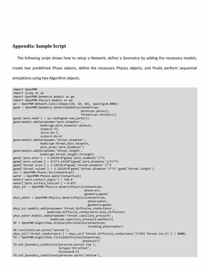
Appendix: Sample Script

The following script shows how to setup a Network, define a Geometry by adding the necessary models,

create two predefined Phase objects, define the necessary Physics objects, and finally perform sequential

simulations using two Algorithm objects.

import OpenPNM import scipy as sp import OpenPNM.Geometry.models as gm import OpenPNM.Physics.models as pm pn = OpenPNM.Network.Cubic(shape=[10, 10, 10], spacing=0.0001) geom = OpenPNM.Geometry.GenericGeometry(network=pn, pores=pn.pores(), throats=pn.throats()) geom['pore.seed'] = sp.rand(geom.num_pores()) geom.models.add(propname='pore.diameter', model=gm.pore_diameter.weibull, shape=2.77, loc=6.9e-7, scale=9.8e-6) geom.models.add(propname='throat.diameter', model=gm.throat_misc.minpore, pore_prop='pore.diameter') geom.models.add(propname='throat.length', model=gm.throat_length.straight) geom['pore.area'] = 3.14159/4*geom['pore.diameter']**2 geom['pore.volume'] = 4/3*3.14159*(geom['pore.diameter']/2)**3 geom['throat.area'] = 3.14159/4*geom['throat.diameter']**2 geom['throat.volume'] = 3.14159/4*geom['throat.diameter']**2* geom['throat.length'] air = OpenPNM.Phases.Air(network=pn) water = OpenPNM.Phases.Water(network=pn) water['pore.contact_angle'] = 110.0 water['pore.surface_tension'] = 0.072 phys_air = OpenPNM.Physics.GenericPhysics(network=pn, phase=air, geometry=geom) phys_water = OpenPNM.Physics.GenericPhysics(network=pn, phase=water, geometry=geom) phys_air.models.add(propname='throat.diffusive_conductance', model=pm.diffusive_conductance.bulk_diffusion) phys_water.models.add(propname='throat.capillary_pressure', model=pm.capillary_pressure.washburn) OP = OpenPNM.Algorithms.OrdinaryPercolation(network=pn, invading_phase=water) OP.run(inlets=pn.pores('bottom')) phys_air['throat.conductance'] = phys_air['throat.diffusive_conductance']*(OP['throat.inv_Pc'] > 8000) FD = OpenPNM.Algorithms.FickianDiffusion(network=pn, phase=air) FD.set_boundary_conditions(pores=pn.pores('top'), bctype='Dirichlet', bcvalue=0.5) FD.set_boundary_conditions(pores=pn.pores('bottom'),

bctype='Dirichlet', bcvalue=0.1) FD.run(conductance='throat.conductance')

Figures

Figure 1: Schematic of random network architecture with pore (node) and throat (bond) numbers labeled. Also shown are the adjacency matrix (bottom left) and incidence matrix (bottom right) representation of this network.

Figure 2: Schematic representation of Core object relationships. Overlap in the vertical direction indicates that objects are associated with the same pores (and or throats), while overlap in the horizontal direction indicates with which Phases each object is associated. Phases by definition don’t overlap with each other but span all pores/throats, Geometry objects span all Phases but only a limited set of pores/throats, and Physics objects exist at the intersection of Phase

and Geometry objects.

Figure 3: Schematic diagram showing the definitions and dimension of a typical pore-throat-pore conduit.

Figure 4: Schematic diagram showing how pore-scale models are associated with Core objects. When the regenerate method of the ModelsDict is called, it

calls the run method of each ModelWrapper in the order they are stored. The values returned from the model are placed into the Core object’s dictionary under the same property name as the model is stored.

Figure 5: 3D rendering of a pore network showing water invading in from bottom (blue) and gas diffusion from top to bottom (yellow to red). The size of the spheres are proportional to the pore diameter. Throats are drawn as thin lines to enhance visualization.