OpenFOAMWorkshop 2014:Effects of grid quality on solution accuracyWritten by J. RhoadsJuly 3, 2014

General InformationThe 9th OpenFOAM Workshop was held in Zagreb, Croatia from June 23-26, 2014. Around 250participants in the workshop took part in a series of presentations, tutorials, and special interestgroups, with the intent on furthering the collective understanding of both OpenFOAM and CFDin general. Of particular interest was the significant discussion in regard to preprocessing–bothin terms of grid generation and grid effects on the solution.

Grid GenerationGrid generation remains a significant challenge for CFD. There are several open source solutionsthat were discussed in varying levels of detail:

• blockMesh - Block structured grids for simple geometries

• snappyHexMesh - Automated hex-core poly mesher with some inflation layer capabilities

• cfMesh - Automated hex-core poly mesher that allows for retaining edges and can subdi-vide first layer of cells to create pseudo boundary layer mesh

• foamyHexMesh - Additional automated poly mesher

Interestingly, all of the open source tools for complex geometries use some sort of cut-cellapproach (for automation purposes) in place of a bottom-up approach similar to that used inPointwise. These methods are commonly favored because of their relative stability/robustness,their ability to handle arbitrarily complex geometries, and their scaling properties when run inparallel using distributed memory.

However, all open source solutions for complex geometries sacrifice control over the surfacemesh and boundary layer cells in favor of automation. Each of the three automated methods havesome form of boundary layer tools, but they all suffer from limitations including overall bound-ary layer thickness, lack of control over initial cell height, and limited robustness of inflationlayers near complex features (such as concave corners). Further, all of these automated solu-tions use discrete representations of the underlying geometry, inherently limiting the surfaceresolution to that of the initial representation. That is, surface curvature information is lost,making grid refinement studies problematic.

Several attendees voiced the opinion that while open source tools are suitable (and indeedquite useful) for rough calculations, some precise, high fidelity simulations require more control

1

2

over the mesh than open source solutions can currently provide. In such applications, accuratelycapturing the physics of the boundary layers is paramount. Having sudden changes in cellorientation, cell thickness, or cell type can introduce significant numerical errors (as discussedfollowing section), which will destroy the integrity of the boundary layer and can compromisethe overall accuracy of the CFD solution. For such applications, a bottom-up approach withexact control over the elements near the viscous surfaces is sometimes preferred in order toreduce grid-induced effects in the simulation results.

Grid Effects on Solution AccuracyIntuitively, the method of discretization can have a clear impact on the accuracy of any sim-ulation. Subdividing the simulation volume with highly skewed, non-orthogonal differentialelements will produce a solution with significant errors because of the numerics employed to ap-proximate the differential equations being studied. From the discussions at the workshop, therewere two primary error-inducing grid effects that were commonly discussed, non-orthogonalityand skewness. However, flow alignment can also have an effect on the simulation accuracy, andwill be discussed briefly.

Test CaseThe error arising from grid effects can easily be seen by considering a simple 2D test caseconsidering purely advective transport of a passive scalar (such as temperature when neglectingbuoyancy and thermal diffusion). This test case was used to investigate both flow-aligned andskewness effects. Once the solution on the domain has been calculated, a local error at position(x, y) can be computed as

Err(x, y) =Tsim(x, y) − T (x, y)

〈T (x, y)〉· 100,

and a global error can be taken to be the standard deviation of this error,

σ =

√1N

∑i, j

(Err(xi, y j)

)2,

which provides a single number to quantify the total error in the solution.It should be noted that a non-linear gradient was necessary in order to see these grid effects,

as a linear profile will be perfectly represented by linear interpolations, thereby introducing nofurther error. However, in physically relevant flows, many non-linear gradients exist due to shearin the flow.

Flow MisalignmentWhen orthogonal cells are perfectly aligned with the flow, only interpolation errors are present inthe solution since all face quantities can be accurately calculated from the cell centers. However,when the flow passes at an angle relative to these orthogonal cells, a numerical mixing processoccurs, resulting in artificial numerical diffusion.

These results suggest that flow misalignment introduces non-negligible numerical diffusion,which can increase the error in the solution by almost an order of magnitude above the baselineinterpolation errors.

www.pointwise.com

Pointwise, Inc.213 S. Jennings Ave.

Fort Worth, TX 76104Tel: 817-377-2807

3

Figure 1: A profile for the passive scalar was applied at the inlet boundary condition, and thesimulation domain was rotated with respect to the flow direction. The evolution of the passivescalar across the domain was then tracked to provide a measure of the numerical diffusion.

Figure 2: Grid misalignment leads to a simple geometrically imposed preferential direction dueto the projected area.

Non-OrthogonalityNon-orthogonality is a significant contributor to error in OpenFOAM because of the way thatgradients are calculated at cell faces. By default, gradients at cell faces are calculated by takingthe difference between values at neighboring cell centers and dividing by the appropriate dis-tance. This results in an approximation for the gradient in the direction of the vector connectingthe two cell centers. However, when a term being computed in the system requires the dot prod-uct of the gradient with the face area, this can introduce significant error due to the misalignedface normal and cell-center vectors, as illustrated in Figure 4.

This term is especially critical for diffusive terms, since the discretization of the Laplacianleads to

µ∇2φ→

∫V∇ · (µ∇φ) dV →

∑f

µ f S f · (∇φ) f ,

www.pointwise.com

Pointwise, Inc.213 S. Jennings Ave.

Fort Worth, TX 76104Tel: 817-377-2807

4

(a) (b)

Figure 3: Solution error for orthogonal mesh at (a) 0 degrees and (b) 20 degrees with respect tothe flow shows appreciable error when not flow-aligned.

where φ represents a quantity being solved for and µ is some diffusivity (be it viscosity, thermaldiffusivity, etc.), and S f represents the directional area of each face, f .

It is possible to correct for this grid effect by increasing nNonOrthogonalCorrectorsin the OpenFOAM fvSolution dictionary. In practice, this begins to contribute significanterrors when the angle between the face normal and cell-center vector is above 70 or 80 degrees.However, the simplistic test case outlined above does not suffer from non-orthogonality effectssince the equations being modeled do not contain a Laplacian term.

Figure 4: Non-orthogonality arises from misalignment between face normal vectors and thevector connecting adjacent cell centers (which represents the approximation for the gradientacross the shared face).

SkewnessSkewness can introduce a significant numerical diffusion and is of particular concern in Open-FOAM due to the methods used to compute fluxes between adjacent cells. The skewCorrectedmethod can help mitigate skewness effects to some degree, but simulated experiments show thatwhile this decreases the errors somewhat, it does not completely eliminate the grid effects fromthe solution.

Skewness is of particular importance for convective derivatives, as these derivatives requirethe value on the face to be computed when calculating the flux to the adjacent cell. This can beseen in the discretization of the convective term,

(v · ∇) φ→∫

V∇ · (vφ) dV →

∑f

S f ·(v fφ f

)

www.pointwise.com

Pointwise, Inc.213 S. Jennings Ave.

Fort Worth, TX 76104Tel: 817-377-2807

5

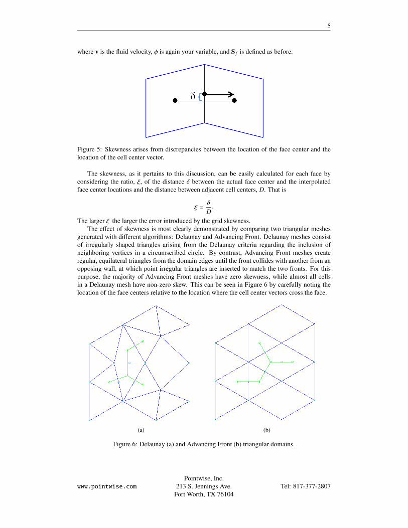
where v is the fluid velocity, φ is again your variable, and S f is defined as before.

Figure 5: Skewness arises from discrepancies between the location of the face center and thelocation of the cell center vector.

The skewness, as it pertains to this discussion, can be easily calculated for each face byconsidering the ratio, ξ, of the distance δ between the actual face center and the interpolatedface center locations and the distance between adjacent cell centers, D. That is

ξ =δ

D.

The larger ξ the larger the error introduced by the grid skewness.The effect of skewness is most clearly demonstrated by comparing two triangular meshes

generated with different algorithms: Delaunay and Advancing Front. Delaunay meshes consistof irregularly shaped triangles arising from the Delaunay criteria regarding the inclusion ofneighboring vertices in a circumscribed circle. By contrast, Advancing Front meshes createregular, equilateral triangles from the domain edges until the front collides with another from anopposing wall, at which point irregular triangles are inserted to match the two fronts. For thispurpose, the majority of Advancing Front meshes have zero skewness, while almost all cellsin a Delaunay mesh have non-zero skew. This can be seen in Figure 6 by carefully noting thelocation of the face centers relative to the location where the cell center vectors cross the face.

(a) (b)

Figure 6: Delaunay (a) and Advancing Front (b) triangular domains.

www.pointwise.com

Pointwise, Inc.213 S. Jennings Ave.

Fort Worth, TX 76104Tel: 817-377-2807

6

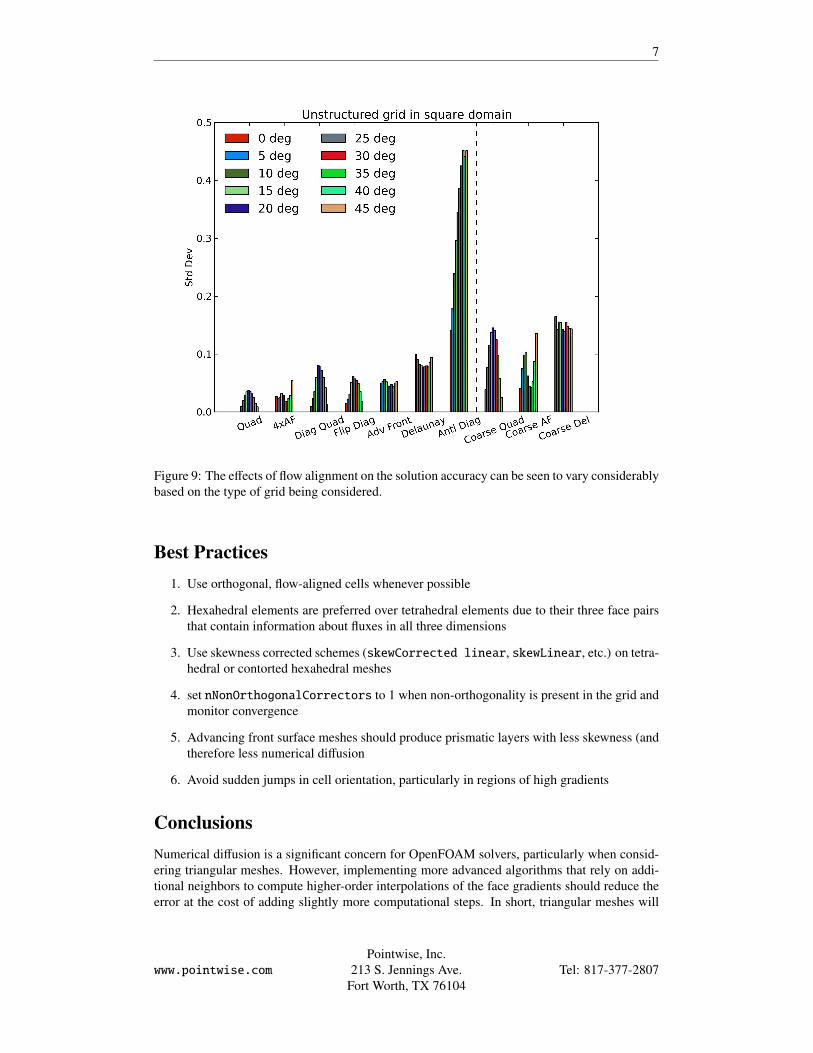
For comparison, the maximum skewness can be calculated for each cell. Comparing a squaredomain populated with these two algorithms as seen in Figure 7 along with the solutions fromthese grids in Figure 8, it is clear that the Delaunay mesh has considerably more skewness andconsequently higher numerical diffusion. However, it should be noted that due to the somewhatrandom orientation of each of the triangles in Delaunay meshes, they are far less sensitive to flowalignment, as seen in Figure 9. The effects of skewness are likely the primary reason tetrahedralgrids tend to be highly diffusive in OpenFOAM with the default solvers.

(a) (b)

Figure 7: Calculated maximum skewness for (a) Delaunay and (b) Advancing Front triangulardomains.

(a) (b)

Figure 8: Calculated error of solution on (a) Delaunay and (b) Advancing Front triangular do-mains.

www.pointwise.com

Pointwise, Inc.213 S. Jennings Ave.

Fort Worth, TX 76104Tel: 817-377-2807

7

Figure 9: The effects of flow alignment on the solution accuracy can be seen to vary considerablybased on the type of grid being considered.

Best Practices1. Use orthogonal, flow-aligned cells whenever possible

2. Hexahedral elements are preferred over tetrahedral elements due to their three face pairsthat contain information about fluxes in all three dimensions

3. Use skewness corrected schemes (skewCorrected linear, skewLinear, etc.) on tetra-hedral or contorted hexahedral meshes

4. set nNonOrthogonalCorrectors to 1 when non-orthogonality is present in the grid andmonitor convergence

5. Advancing front surface meshes should produce prismatic layers with less skewness (andtherefore less numerical diffusion

6. Avoid sudden jumps in cell orientation, particularly in regions of high gradients

ConclusionsNumerical diffusion is a significant concern for OpenFOAM solvers, particularly when consid-ering triangular meshes. However, implementing more advanced algorithms that rely on addi-tional neighbors to compute higher-order interpolations of the face gradients should reduce theerror at the cost of adding slightly more computational steps. In short, triangular meshes will

www.pointwise.com

Pointwise, Inc.213 S. Jennings Ave.

Fort Worth, TX 76104Tel: 817-377-2807

8

work in OpenFOAM, but the presence of numerical diffusion must be taken into account wheninterpreting the results.

Further work investigating three-dimensional diffusion on tetrahedral grids may shed morelight on the problem at hand and suggest ways to improve the quality of solutions obtains fromtetrahedral grids. It should be noted that tetrahedra suffer from a potentially limiting geometricconstraint when computing higher-order interpolations of gradients. That is to say, it is possiblefor all of the face neighbors of a tetrahedral element to lie within the same plane. In such asituation, including the face neighbors will not provide any information about the gradient inthe third dimension. For this reason, it may be necessary to not only include face-neighbors, butedge neighbors as well.

Because of the formulations in OpenFOAM, hex-dominant or polyhedral meshes have fewerrestrictions in terms of the numerics. However, the flow field in the boundary layer must also beaccurately captured by the grid, which poses a challenge to top-down preprocessing approaches.As commonly concluded in CFD, the solution comes down to the mesh.

Additional Resources• http://sourceforge.net/projects/openfoam-extend/files/OpenFOAM_Workshops/

• http://openfoamwiki.net/index.php/Handy_links

• http://openfoamworkshop.org/index.html

www.pointwise.com

Pointwise, Inc.213 S. Jennings Ave.

Fort Worth, TX 76104Tel: 817-377-2807