University of Birmingham Assessing the relative importance ...
Biogeosciences, 10, 2379–2392, 2013www.biogeosciences.net/10/2379/2013/doi:10.5194/bg-10-2379-2013© Author(s) 2013. CC Attribution 3.0 License.
EGU Journal Logos (RGB)
Advances in Geosciences
Open A
ccess
Natural Hazards and Earth System
Sciences
Open A
ccess
Annales Geophysicae
Open A
ccess
Nonlinear Processes in Geophysics
Open A
ccess
Atmospheric Chemistry
and Physics
Open A
ccess
Atmospheric Chemistry
and Physics
Open A
ccess
Discussions
Atmospheric Measurement
Techniques
Open A
ccess
Atmospheric Measurement
Techniques
Open A
ccess
Discussions
Biogeosciences
Open A
ccess
Open A
ccess
BiogeosciencesDiscussions
Climate of the Past
Open A
ccess
Open A
ccess
Climate of the Past
Discussions
Earth System Dynamics
Open A
ccess
Open A
ccess
Earth System Dynamics
Discussions
GeoscientificInstrumentation
Methods andData Systems
Open A
ccess
GeoscientificInstrumentation
Methods andData Systems
Open A
ccess
Discussions
GeoscientificModel Development
Open A
ccess
Open A
ccess
GeoscientificModel Development
Discussions
Hydrology and Earth System
Sciences
Open A
ccess
Hydrology and Earth System
Sciences
Open A
ccess
Discussions
Ocean Science
Open A
ccess
Open A
ccess
Ocean ScienceDiscussions
Solid Earth
Open A
ccess
Open A
ccess
Solid EarthDiscussions
The Cryosphere
Open A
ccess
Open A
ccess
The CryosphereDiscussions
Natural Hazards and Earth System
SciencesO
pen Access
Discussions
The relative importance of decomposition and transportmechanisms in accounting for soil organic carbon profiles
B. Guenet1,2, T. Eglin1, N. Vasilyeva3, P. Peylin1, P. Ciais1, and C. Chenu3
1Laboratoire des Sciences du Climat et de l’Environnement, UMR8212, CEA-CNRS-UVSQ, 91191 Gif-sur-Yvette, France2Department of Biology, University of Antwerpen, Universiteitsplein 1, 2610, Wilrijk, Belgium3AgroParisTech, UPMC-CNRS-AgroParisTech UMR Bioemco7618, 78850 Thiverval-Grignon, France
Correspondence to:B. Guenet ([email protected])
Received: 5 September 2012 – Published in Biogeosciences Discuss.: 15 October 2012Revised: 8 March 2013 – Accepted: 14 March 2013 – Published: 10 April 2013
Abstract. Soil is the major terrestrial reservoir of carbonand a substantial part of this carbon is stored in deep lay-ers, typically deeper than 50 cm below the surface. Severalstudies underlined the quantitative importance of this deepsoil organic carbon (SOC) pool and models are needed tobetter understand this stock and its evolution under climateand land-uses changes. In this study, we tested and comparedthree simple theoretical models of vertical transport for SOCagainst SOC profiles measurements from a long-term barefallow experiment carried out by the Central-ChernozemState Natural Biosphere Reserve in the Kursk Region of Rus-sia. The transport schemes tested are diffusion, advection andboth diffusion and advection. They are coupled to three dif-ferent formulations of soil carbon decomposition kinetics.The first formulation is a first order kinetics widely usedin global SOC decomposition models; the second one, so-called “priming” model, links SOC decomposition rate to theamount of fresh organic matter, representing the substrate in-teractions. The last one is also a first order kinetics, but SOCis split into two pools. Field data are from a set of three barefallow plots where soil received no input during the past 20,26 and 58 yr, respectively. Parameters of the models were op-timised using a Bayesian method. The best results are ob-tained when SOC decomposition is assumed to be controlledby fresh organic matter (i.e., the priming model). In com-parison to the first-order kinetic model, the priming modelreduces the overestimation in the deep layers. We also ob-served that the transport scheme that improved the fit withthe data depended on the soil carbon mineralisation formula-tion chosen. When soil carbon decomposition was modelledto depend on the fresh organic matter amount, the transport
mechanism which improved best the fit to the SOC profiledata was the model representing both advection and diffu-sion. Interestingly, the older the bare fallow is, the lesser theneed for diffusion is, suggesting that stabilised carbon maynot be transported within the profile by the same mechanismsthan more labile carbon.
1 Introduction
Soils are the major reservoir of terrestrial organic carbon (C)representing more than twice the amount of C stored in theatmosphere and three times the amount of C stored in ter-restrial vegetation (Schimel, 1995; Schlesinger, 1990; MEA,2005). In spite of the importance of the stock, the dynam-ics of soil C is not deeply understood (Sugden et al., 2004).Soil scientists have mainly focused on the surface horizons(Lueken et al., 1962; Sparling et al., 1982; Wu et al., 1993),which were considered to be the only depth of the soil whichcan emit CO2 to the atmosphere in significant amounts. How-ever, recent studies have shown that the amount of C storedin the deep layers (below 30 cm) could represent between 30and 63 % of the total amount of soil C (Batjes, 1996; Jobbagyand Jackson, 2000; Tarnocai et al., 2009). Consequently, in-creasing attention has been paid to deep soil C and in par-ticular to its dynamics (Fontaine et al., 2007; Salome et al.,2010; Rumpel et al., 2010; Sanaullah et al., 2010).
Transport mechanisms of soil C into deep layers is stillnot well understood. The models applied at site-level gener-ally represent both vertical advection and diffusion (Elzeinand Balesdent, 1995; Bruun et al., 2007; Braakhekke et al.,
Published by Copernicus Publications on behalf of the European Geosciences Union.

2380 B. Guenet et al.: Decomposition and transport mechanisms in accounting for SOC profiles
2011), but models also exist with only advection (Feng etal., 1999; Dorr and Munnich, 1989; Jenkinson and Coleman,2008) or only diffusion (O’Brien and Stout, 1978; Wynn etal., 2005). To our knowledge, no formal and comprehen-sive comparison of the three transport mechanisms combinedto different representations of decomposition has been per-formed, even if Bruun et al. (2007) suggested that the rep-resentation of both advection and diffusion mechanisms im-proved their model for a sandy soil. However, they compareda model with both advection and diffusion to an advection-only model, but they do not compare these models with adiffusion-only model.
The Soil Organic Matter (SOM) decomposition mecha-nisms proposed as equations that can be encapsulated inmodels are also very diverse (for review see, Manzoni andPorporato, 2009; Wutzler and Reichstein, 2008). Within allthese approaches, the most used formulation is the first orderkinetics as in CENTURY (Parton et al., 1988) or in RothC(Coleman and Jenkinson, 1996). In this formulation, the de-cay of each SOM pool is proportional to the pool’s size,thereby considering that there are no interactions betweentwo decomposing pools.
In particular, within the fourth Assessment Report (AR4)of the Intergovernmental Panel on Climate Change (IPCC),the climate-carbon models used during the Coupled CarbonCycle Climate Model Intercomparison Project (C4MIP) rep-resented the SOM decomposition with first order kinetics(Friedlingstein et al., 2006). This approach is now criticised(Fontaine and Barot, 2005; Wutzler and Reichstein, 2008),in particular, for its incapacity to represent the relationshipexisting between Fresh Organic Matter (FOM) inputs (e.g.,roots exudates, litter, etc.) and the mineralisation of the SOM.This interaction seems to be a major mechanism of SOM sta-bilisation in the deep soil layers (Fontaine et al., 2007) evenif it could be soil dependent (Salome et al., 2010). However,here again, to our knowledge no clear comparison betweenfirst order kinetics and any of the alternative decomposi-tion formulations linking FOM input to SOM mineralisationhas been done.
To study how FOM may possibly interact with SOM min-eralisation, experimental sites such as long-term bare fallowsoils are interesting experiments. Instead of the complexity ofreal soils where FOM is permanently added and depends onecosystem properties, in a bare fallow, the input of FOM hasbeen stopped. Consequently, the relationship between FOMinput and SOM mineralisation is switched-off in the bare fal-low, whereas it remains switched on in the control plots. Inour case, we used bare fallow soils sampled at different yearsincluding periods where FOM was assumed to be still avail-able, because it had not yet decomposed, and periods whereFOM stock was assumed to be close to zero (Barre et al.,2010).
In this study, we developed a suite of conceptual modelsto compare the three main transport schemes (advection onlyTA ; diffusion only TD, both togetherTAD) proposed in the
literature using measurement of soil C profiles obtained in along-term bare fallow and a control plot near Kursk in Rus-sia. We also aimed to cross the three transport schemes withthe different formulations used to describe SOM mineralisa-tion: a first order kinetics without relationship between FOMinput and SOM mineralisation and a formulation inspiredfrom Wutzler and Reichstein (2008) where the relationshipbetween FOM input and SOM mineralisation is represented.Moreover, we used a three pools model with decompositionbased on first order kinetics with both advection and diffu-sion to better understand how increasing the number of pa-rameters may improve the fit with the data. We first optimisedthe parameters of each of the seven possible models, usingthe observed soil carbon profiles and a statistical optimisa-tion method (least square minimization). We then comparedthe model outputs with measurements from all soil carbonprofiles from the bare fallow.
2 Materials and methods
2.1 The Kursk long-term field experiment data
2.1.1 Site and soil plots description
Soils were sampled at the long-term field experiment theCentral-Chernozem State Natural Biosphere Reserve namedafter V. V. Alekhin in the Kursk Region of Russia. The cli-matic zone is a forest steppe temperate, moderately coldwith a mean annual precipitation of 587 mm and a meanannual air temperature of 5.4◦C (Central-Chernozem StateNatural Biosphere Reserve, 1947–1997). The soil is a HaplicChernozem defined as a silty loam Haplic Luvisol followingthe FAO classification. Two long-term plots were sampledwithin the site located in the Streletskyi section of the re-serve at 51◦ N, 36◦ E, about 18 km south of the city of Kursk(Vinogradov, 1984).
The first plot is a long-term bare fallow soil where no freshinput entered the soils since 1947. The soil was weeded man-ually and tilled every year by horse traction at a depth cor-responding to 17–18 cm until the middle of the 1970s andthen using a machine at a depth of 22–24 cm. Before the startof the experiment, the soil was under a natural steppe thathad been under hay-harvest and pasture for at least the lastfour centuries. The second plot is geographically close to thefirst one (about 50 m). It is the same natural steppe that hasbeen absolutely reserved since the establishment of the Re-serve in 1935 (Afanasyeva, 1966). It is a natural steppe since1935 and was used previously for pasture. Dominant plantspecies are meadow bromegrass (Bromus ripariusRehm.),wild oats (Stipa pennataL.), narrow-leaved meadow grass(Poa angustifoliaL.), intermediate wheatgrass (Elytrigia in-termedia (Host) Nevski), meadowsweet rose (Filipendulavulgaris Moench), and green strawberry (Fragaria viridis
Biogeosciences, 10, 2379–2392, 2013 www.biogeosciences.net/10/2379/2013/
B. Guenet et al.: Decomposition and transport mechanisms in accounting for SOC profiles 2381
Duch.). This soil is considered as a control (undisturbed) plotfor the bare fallow experiment.
2.1.2 Soil sampling and carbon measurements
Soils were sampled at the bare fallow plot in 1967, 1973 and2005 at depths of every 10 cm down to 150 cm. The soil of thesteppe was sampled in 2006 at depths of every 10 cm downto 150 cm. Soils were sampled five times in the steppe, in thebare fallow in 1967 and 2005 and three times in 1973. Thecorresponding profiles are hereafter called 20YBF, 26YBFand 58YBF for the bare fallow soil sampled in 1967, 1973and 2005, respectively (i.e., after 20, 26 and 58 yr of bare fal-low) and S for the steppe. C contents obtained by the Tyurinmethod in 1967 and 1973 are corrected by a multiplicativefactor 1.13, determined particularly for this soil to match drycombustion method and, thus, avoid any underestimation ofthe C content (Vasilyeva et al., 2013). In years 2005 and2006, soil C was measured by dry combustion (Vario Ele-mentar, Analysensysteme, Hanau, Germany).
The bulk density of the soils was first measured for eachlayer until 120 cm depth in 1959, and this measurement wasrepeated in 2002 for the bare fallow and for the steppe plots.To take into account the difference in bulk density betweenthe samples, the C stocks are expressed in kg C m−2 as fol-lows:
Cstock= TOC× BD × h (1)
with TOC being the total organic carbon content of the layerconsidered, expressed in kg C kg−1 soil, BD the bulk densityexpressed in kg soil m−3 and h the layer height expressedin m. Since bulk densities are available only until 120 cm,the soil profiles in kg C m−2 are calculated only until 120 cmdepth. The bulk densities measured in 1959 are used for thesoil layer sampled in 1967 and in 1973, whereas the bulk den-sities measured in 2002 are used for the soil layers sampled in2005 and in 2006. The chronosequence used in this study isinteresting because it follows the decrease of the FOM stockfrom an equilibrium to another. Indeed, Barre et al. (2010)showed that FOM stock are generally close to zero after 40 yrof bare fallow. Thus, FOM stock is assumed to be high andat the equilibrium for the steppe and close to zero, but also atthe equilibrium for the 58YBF. The 20YBF and the 26YBFprofiles being intermediate situations.
2.2 Soil carbon decomposition models
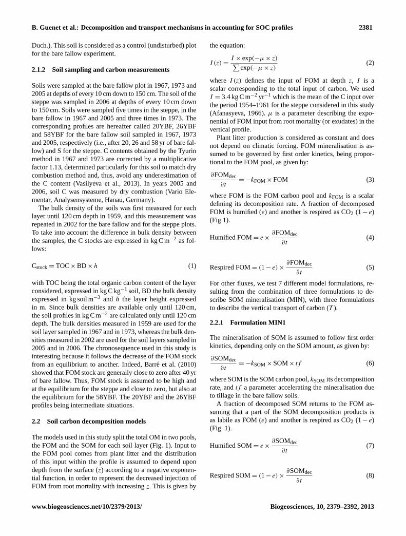
The models used in this study split the total OM in two pools,the FOM and the SOM for each soil layer (Fig. 1). Input tothe FOM pool comes from plant litter and the distributionof this input within the profile is assumed to depend upondepth from the surface (z) according to a negative exponen-tial function, in order to represent the decreased injection ofFOM from root mortality with increasingz. This is given by
the equation:
I (z) =I × exp(−µ × z)∑
exp(−µ × z)(2)
where I (z) defines the input of FOM at depthz, I is ascalar corresponding to the total input of carbon. We usedI = 3.4 kg C m−2 yr−1 which is the mean of the C input overthe period 1954–1961 for the steppe considered in this study(Afanasyeva, 1966).µ is a parameter describing the expo-nential of FOM input from root mortality (or exudates) in thevertical profile.
Plant litter production is considered as constant and doesnot depend on climatic forcing. FOM mineralisation is as-sumed to be governed by first order kinetics, being propor-tional to the FOM pool, as given by:
∂FOMdec
∂t= −kFOM × FOM (3)
where FOM is the FOM carbon pool andkFOM is a scalardefining its decomposition rate. A fraction of decomposedFOM is humified (e) and another is respired as CO2 (1− e)(Fig 1).
Humified FOM= e ×∂FOMdec
∂t(4)
Respired FOM= (1− e) ×∂FOMdec
∂t(5)
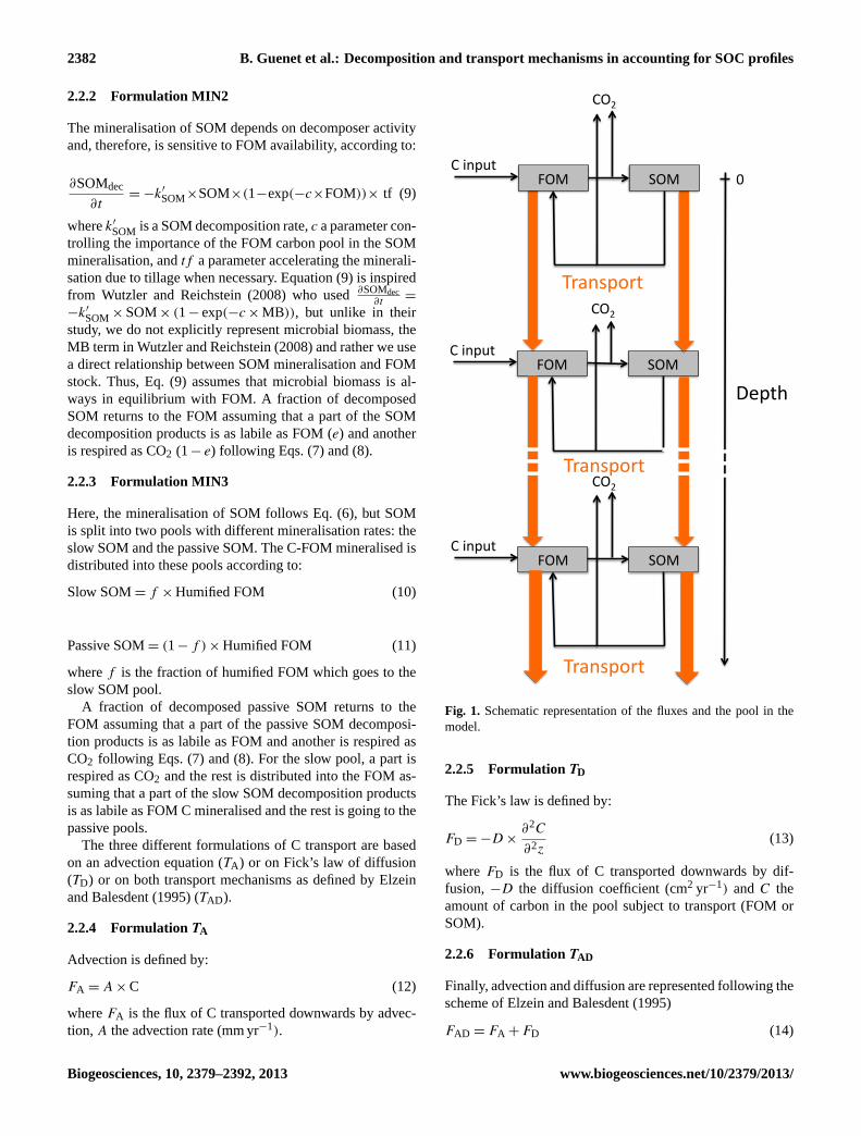
For other fluxes, we test 7 different model formulations, re-sulting from the combination of three formulations to de-scribe SOM mineralisation (MIN), with three formulationsto describe the vertical transport of carbon (T ).
2.2.1 Formulation MIN1
The mineralisation of SOM is assumed to follow first orderkinetics, depending only on the SOM amount, as given by:
∂SOMdec
∂t= −kSOM× SOM× tf (6)
where SOM is the SOM carbon pool,kSOM its decompositionrate, andtf a parameter accelerating the mineralisation dueto tillage in the bare fallow soils.
A fraction of decomposed SOM returns to the FOM as-suming that a part of the SOM decomposition products isas labile as FOM (e) and another is respired as CO2 (1− e)(Fig. 1).
Humified SOM= e ×∂SOMdec
∂t(7)
Respired SOM= (1− e) ×∂SOMdec
∂t(8)
www.biogeosciences.net/10/2379/2013/ Biogeosciences, 10, 2379–2392, 2013
2382 B. Guenet et al.: Decomposition and transport mechanisms in accounting for SOC profiles
2.2.2 Formulation MIN2
The mineralisation of SOM depends on decomposer activityand, therefore, is sensitive to FOM availability, according to:
∂SOMdec
∂t= −k′
SOM×SOM×(1−exp(−c×FOM))× tf (9)
wherek′
SOM is a SOM decomposition rate,c a parameter con-trolling the importance of the FOM carbon pool in the SOMmineralisation, andtf a parameter accelerating the minerali-sation due to tillage when necessary. Equation (9) is inspiredfrom Wutzler and Reichstein (2008) who used∂SOMdec
∂t=
−k′
SOM× SOM× (1− exp(−c × MB)), but unlike in theirstudy, we do not explicitly represent microbial biomass, theMB term in Wutzler and Reichstein (2008) and rather we usea direct relationship between SOM mineralisation and FOMstock. Thus, Eq. (9) assumes that microbial biomass is al-ways in equilibrium with FOM. A fraction of decomposedSOM returns to the FOM assuming that a part of the SOMdecomposition products is as labile as FOM (e) and anotheris respired as CO2 (1− e) following Eqs. (7) and (8).
2.2.3 Formulation MIN3
Here, the mineralisation of SOM follows Eq. (6), but SOMis split into two pools with different mineralisation rates: theslow SOM and the passive SOM. The C-FOM mineralised isdistributed into these pools according to:
Slow SOM= f × Humified FOM (10)
Passive SOM= (1− f ) × Humified FOM (11)
wheref is the fraction of humified FOM which goes to theslow SOM pool.
A fraction of decomposed passive SOM returns to theFOM assuming that a part of the passive SOM decomposi-tion products is as labile as FOM and another is respired asCO2 following Eqs. (7) and (8). For the slow pool, a part isrespired as CO2 and the rest is distributed into the FOM as-suming that a part of the slow SOM decomposition productsis as labile as FOM C mineralised and the rest is going to thepassive pools.
The three different formulations of C transport are basedon an advection equation (TA) or on Fick’s law of diffusion(TD) or on both transport mechanisms as defined by Elzeinand Balesdent (1995) (TAD).
2.2.4 FormulationTA
Advection is defined by:
FA = A × C (12)
whereFA is the flux of C transported downwards by advec-tion, A the advection rate (mm yr−1).
FOM SOM C input
Transport
CO2
FOM SOM C input
Transport
CO2
Depth
FOM SOM C input
CO2
Transport
0
Fig. 1. Schematic representation of the fluxes and the pool in themodel.
2.2.5 FormulationTD
The Fick’s law is defined by:
FD = −D ×∂2C
∂2z(13)
whereFD is the flux of C transported downwards by dif-fusion, −D the diffusion coefficient (cm2 yr−1) andC theamount of carbon in the pool subject to transport (FOM orSOM).
2.2.6 FormulationTAD
Finally, advection and diffusion are represented following thescheme of Elzein and Balesdent (1995)
FAD = FA + FD (14)
Biogeosciences, 10, 2379–2392, 2013 www.biogeosciences.net/10/2379/2013/

B. Guenet et al.: Decomposition and transport mechanisms in accounting for SOC profiles 2383
FOM decomposi-on following first order
kine-c
SOM decomposi-on following first order
kine-c (MIN1)
SOM decomposi-on controlled by FOM availability (MIN2)
Advec-on (TA)
Diffusion (TD)
Advec-on + Diffusion
(TAD)
Advec-on (TA)
Diffusion (TD)
Advec-on + Diffusion
(TAD)
MIN1-TA MIN1-TD MIN1-TAD MIN2-TA MIN2-TD MIN2-TAD
SOM described by two pools with SOM decomposi-on following first order kine-c (MIN3)
Advec-on + Diffusion
(TAD)
MIN3-TAD
Fig. 2.Presentation of the seven formulations used in this study.
FAD = A × C − D ×∂2C
∂2z(15)
whereFAD is the flux of C transported downwards by ad-vection and diffusion,A the advection rate,−D the diffu-sion coefficient andC the amount of carbon in the pool sub-ject to transport. We finally build the seven different modelsby forming pair of (MIN,T ) formulations as illustrated byFig. 2. Thus, the FOM and SOM pools dynamics correspondto:
∂FOM
∂t∂z= I +
∂FX
∂z+ e ×
∂SOMdec
∂t−
∂FOMdec
∂t(16)
∂SOM
∂t∂z=
∂FX
∂z+ e ×
∂FOMdec
∂t−
∂SOMdec
∂t(17)
All the models were developed using R 2.11.1 and run at ayearly time step. The models run from the ground (0 cm) un-til 200 cm and the vertical resolution is 5 mm for each layer.To compare with the data, C stocks are then summed each20 layers to obtain 10 cm layers. Moreover only the layersuntil 120 cm are used since the data could be converted inkg C m−2 only until 120 cm. The equations were solved us-ing the deSolve library (Soetaert et al., 2010). This librarysolves a system of ordinary differential equations resultingfrom one dimensional partial differential equations that havebeen converted to ordinary differential equations by numeri-cal differencing. We run the models with the steppe condition(i.e., with input of FOM) during 2000 yr to reach the equilib-rium. The steppe was assumed to be at the equilibrium and
we used the C stocks obtained after the 2000 yr run for thesteppe. Then we run the model for 58 yr without FOM inputto reproduce the 58YBF plots condition. From this run, weextracted the data after 20 and 26 yr to reproduce the 20YBFand 26YBF plots condition, respectively.
2.3 Parameter optimisation
The 10 parameters used for each simulation are listed in Ta-ble 1. Eight of them are optimised for each model using aBayesian inversion method with priors (see Tarantola, 1987)against the entire dataset (48 data points, i.e., 12 for each pro-file), with a statistical approach based on a Bayesian frame-work (Tarantola, 1987). Our approach is based on Santarenet al. (2007). The optimal parameter set corresponds to theminimum of the cost function
J (x) =1
2
[(y − H(x))t R−1 (y − H(x)) + (x − xb)
t P −1b (x − xb)
](18)
and contains both the mismatch between modelled and ob-served fluxes and the mismatch between prior and optimisedparameters.x is the vector of unknown parameters,xb theprior parameters,H(x) the model outputs andy the vectorof observations.Pb describes the prior parameter error vari-ances/covariances, whileR contains the prior data error vari-ances/covariances.
An efficient gradient-based iterative algorithm, called L-BFGS-B (Zhu et al., 1995) was used to minimise the costfunction. This algorithm prescribes a range of values for eachparameter. At each iteration, the gradient of the cost func-tion J (x) is computed, with respect to all the parameters.The L-BFGS-B algorithm does not provide uncertainties or
www.biogeosciences.net/10/2379/2013/ Biogeosciences, 10, 2379–2392, 2013
2384 B. Guenet et al.: Decomposition and transport mechanisms in accounting for SOC profiles
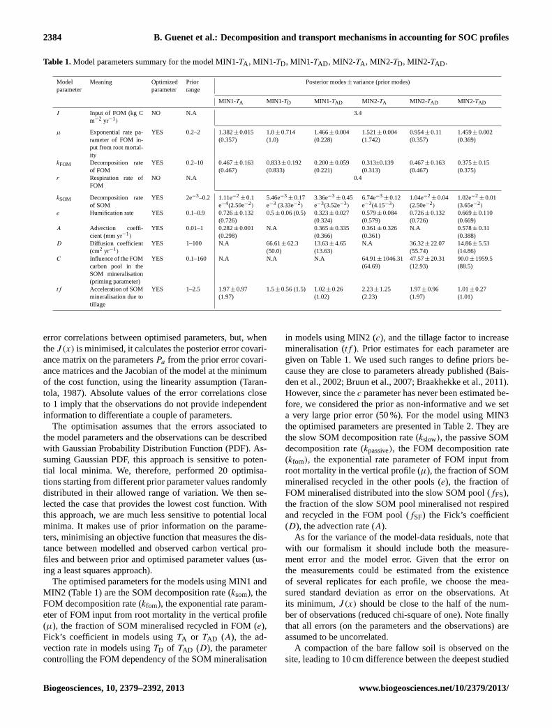
Table 1.Model parameters summary for the model MIN1-TA , MIN1-TD, MIN1-TAD , MIN2-TA , MIN2-TD, MIN2-TAD .
Model Meaning Optimized Prior Posterior modes± variance (prior modes)parameter parameter range
MIN1-TA MIN1-TD MIN1-TAD MIN2-TA MIN2-TAD MIN2-TAD
I Input of FOM (kg Cm−2 yr−1)
NO N.A 3.4
µ Exponential rate pa-rameter of FOM in-put from root mortal-ity
YES 0.2–2 1.382± 0.015(0.357)
1.0± 0.714(1.0)
1.466± 0.004(0.228)
1.521± 0.004(1.742)
0.954± 0.11(0.357)
1.459± 0.002(0.369)
kFOM Decomposition rateof FOM
YES 0.2–10 0.467± 0.163(0.467)
0.833± 0.192(0.833)
0.200± 0.059(0.221)
0.313±0.139(0.313)
0.467± 0.163(0.467)
0.375± 0.15(0.375)
r Respiration rate ofFOM
NO N.A 0.4
kSOM Decomposition rateof SOM
YES 2e−3–0.2 1.11e−2± 0.1
e−4(2.50e−2)
5.46e−3± 0.17
e−3 (3.33e−2)
3.36e−3± 0.45
e−3(3.52e−3)
6.74e−3± 0.12
e−3(4.15−3)
1.04e−2± 0.04
(2.50e−2)
1.02e−2± 0.01
(3.65e−2)
e Humification rate YES 0.1–0.9 0.726± 0.132(0.726)
0.5± 0.06 (0.5) 0.323± 0.027(0.324)
0.579± 0.084(0.579)
0.726± 0.132(0.726)
0.669± 0.110(0.669)
A Advection coeffi-cient (mm yr−1)
YES 0.01–1 0.282± 0.001(0.298)
N.A 0.365± 0.335(0.366)
0.361± 0.326(0.361)
N.A 0.578± 0.31(0.388)
D Diffusion coefficient(cm2 yr−1)
YES 1–100 N.A 66.61± 62.3(50.0)
13.63± 4.65(13.63)
N.A 36.32± 22.07(55.74)
14.86± 5.53(14.86)
C Influence of the FOMcarbon pool in theSOM mineralisation(priming parameter)
YES 0.1–160 N.A N.A N.A 64.91± 1046.31(64.69)
47.57± 20.31(12.93)
90.0± 1959.5(88.5)
tf Acceleration of SOMmineralisation due totillage
YES 1–2.5 1.97± 0.97(1.97)
1.5± 0.56 (1.5) 1.02± 0.26(1.02)
2.23± 1.25(2.23)
1.97± 0.96(1.97)
1.01± 0.27(1.01)
error correlations between optimised parameters, but, whentheJ (x) is minimised, it calculates the posterior error covari-ance matrix on the parametersPa from the prior error covari-ance matrices and the Jacobian of the model at the minimumof the cost function, using the linearity assumption (Taran-tola, 1987). Absolute values of the error correlations closeto 1 imply that the observations do not provide independentinformation to differentiate a couple of parameters.
The optimisation assumes that the errors associated tothe model parameters and the observations can be describedwith Gaussian Probability Distribution Function (PDF). As-suming Gaussian PDF, this approach is sensitive to poten-tial local minima. We, therefore, performed 20 optimisa-tions starting from different prior parameter values randomlydistributed in their allowed range of variation. We then se-lected the case that provides the lowest cost function. Withthis approach, we are much less sensitive to potential localminima. It makes use of prior information on the parame-ters, minimising an objective function that measures the dis-tance between modelled and observed carbon vertical pro-files and between prior and optimised parameter values (us-ing a least squares approach).
The optimised parameters for the models using MIN1 andMIN2 (Table 1) are the SOM decomposition rate (ksom), theFOM decomposition rate (kfom), the exponential rate param-eter of FOM input from root mortality in the vertical profile(µ), the fraction of SOM mineralised recycled in FOM (e),Fick’s coefficient in models usingTA or TAD (A), the ad-vection rate in models usingTD of TAD (D), the parametercontrolling the FOM dependency of the SOM mineralisation
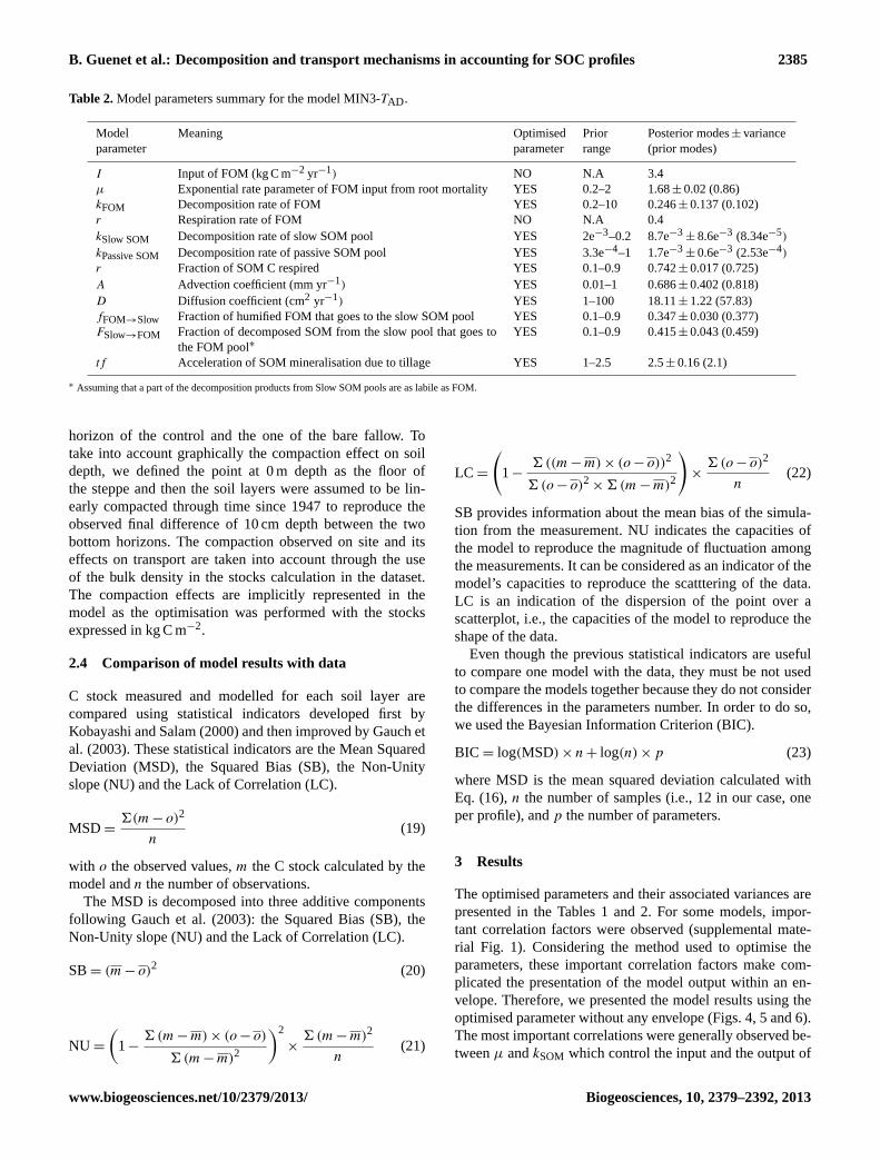
in models using MIN2 (c), and the tillage factor to increasemineralisation (tf ). Prior estimates for each parameter aregiven on Table 1. We used such ranges to define priors be-cause they are close to parameters already published (Bais-den et al., 2002; Bruun et al., 2007; Braakhekke et al., 2011).However, since thec parameter has never been estimated be-fore, we considered the prior as non-informative and we seta very large prior error (50 %). For the model using MIN3the optimised parameters are presented in Table 2. They arethe slow SOM decomposition rate (kslow), the passive SOMdecomposition rate (kpassive), the FOM decomposition rate(kfom), the exponential rate parameter of FOM input fromroot mortality in the vertical profile (µ), the fraction of SOMmineralised recycled in the other pools (e), the fraction ofFOM mineralised distributed into the slow SOM pool (fFS),the fraction of the slow SOM pool mineralised not respiredand recycled in the FOM pool (fSF) the Fick’s coefficient(D), the advection rate (A).
As for the variance of the model-data residuals, note thatwith our formalism it should include both the measure-ment error and the model error. Given that the error onthe measurements could be estimated from the existenceof several replicates for each profile, we choose the mea-sured standard deviation as error on the observations. Atits minimum,J (x) should be close to the half of the num-ber of observations (reduced chi-square of one). Note finallythat all errors (on the parameters and the observations) areassumed to be uncorrelated.
A compaction of the bare fallow soil is observed on thesite, leading to 10 cm difference between the deepest studied
Biogeosciences, 10, 2379–2392, 2013 www.biogeosciences.net/10/2379/2013/
B. Guenet et al.: Decomposition and transport mechanisms in accounting for SOC profiles 2385
Table 2.Model parameters summary for the model MIN3-TAD .
Model Meaning Optimised Prior Posterior modes± varianceparameter parameter range (prior modes)
I Input of FOM (kg C m−2 yr−1) NO N.A 3.4µ Exponential rate parameter of FOM input from root mortality YES 0.2–2 1.68± 0.02 (0.86)kFOM Decomposition rate of FOM YES 0.2–10 0.246± 0.137 (0.102)r Respiration rate of FOM NO N.A 0.4kSlow SOM Decomposition rate of slow SOM pool YES 2e−3–0.2 8.7e−3
± 8.6e−3 (8.34e−5)
kPassive SOM Decomposition rate of passive SOM pool YES 3.3e−4–1 1.7e−3± 0.6e−3 (2.53e−4)
r Fraction of SOM C respired YES 0.1–0.9 0.742± 0.017 (0.725)A Advection coefficient (mm yr−1) YES 0.01–1 0.686± 0.402 (0.818)D Diffusion coefficient (cm2 yr−1) YES 1–100 18.11± 1.22 (57.83)fFOM→Slow Fraction of humified FOM that goes to the slow SOM pool YES 0.1–0.9 0.347± 0.030 (0.377)FSlow→FOM Fraction of decomposed SOM from the slow pool that goes to
the FOM pool∗YES 0.1–0.9 0.415± 0.043 (0.459)
tf Acceleration of SOM mineralisation due to tillage YES 1–2.5 2.5± 0.16 (2.1)
∗ Assuming that a part of the decomposition products from Slow SOM pools are as labile as FOM.
horizon of the control and the one of the bare fallow. Totake into account graphically the compaction effect on soildepth, we defined the point at 0 m depth as the floor ofthe steppe and then the soil layers were assumed to be lin-early compacted through time since 1947 to reproduce theobserved final difference of 10 cm depth between the twobottom horizons. The compaction observed on site and itseffects on transport are taken into account through the useof the bulk density in the stocks calculation in the dataset.The compaction effects are implicitly represented in themodel as the optimisation was performed with the stocksexpressed in kg C m−2.
2.4 Comparison of model results with data
C stock measured and modelled for each soil layer arecompared using statistical indicators developed first byKobayashi and Salam (2000) and then improved by Gauch etal. (2003). These statistical indicators are the Mean SquaredDeviation (MSD), the Squared Bias (SB), the Non-Unityslope (NU) and the Lack of Correlation (LC).
MSD =6(m − o)2
n(19)
with o the observed values,m the C stock calculated by themodel andn the number of observations.
The MSD is decomposed into three additive componentsfollowing Gauch et al. (2003): the Squared Bias (SB), theNon-Unity slope (NU) and the Lack of Correlation (LC).
SB= (m − o)2 (20)
NU =
(1−
6(m − m) × (o − o)
6 (m − m)2
)2
×6(m − m)2
n(21)
LC =
(1−
6((m − m) × (o − o))2
6(o − o)2× 6(m − m)2
)×
6(o − o)2
n(22)
SB provides information about the mean bias of the simula-tion from the measurement. NU indicates the capacities ofthe model to reproduce the magnitude of fluctuation amongthe measurements. It can be considered as an indicator of themodel’s capacities to reproduce the scatttering of the data.LC is an indication of the dispersion of the point over ascatterplot, i.e., the capacities of the model to reproduce theshape of the data.
Even though the previous statistical indicators are usefulto compare one model with the data, they must be not usedto compare the models together because they do not considerthe differences in the parameters number. In order to do so,we used the Bayesian Information Criterion (BIC).
BIC = log(MSD) × n + log(n) × p (23)
where MSD is the mean squared deviation calculated withEq. (16),n the number of samples (i.e., 12 in our case, oneper profile), andp the number of parameters.
3 Results
The optimised parameters and their associated variances arepresented in the Tables 1 and 2. For some models, impor-tant correlation factors were observed (supplemental mate-rial Fig. 1). Considering the method used to optimise theparameters, these important correlation factors make com-plicated the presentation of the model output within an en-velope. Therefore, we presented the model results using theoptimised parameter without any envelope (Figs. 4, 5 and 6).The most important correlations were generally observed be-tweenµ andkSOM which control the input and the output of
www.biogeosciences.net/10/2379/2013/ Biogeosciences, 10, 2379–2392, 2013

2386 B. Guenet et al.: Decomposition and transport mechanisms in accounting for SOC profiles
Table 3.Bayesian Information Criterion (BIC).
MIN1-TA MIN1-TD MIN1-TAD MIN2-TA MIN2-TD MIN2-TAD MIN3-TAD
Entire dataset 181.4 179.3 173.6 196.2 182.1 177.7 200.5Steppe 63.3 39.2 57.0 67.2 59.5 61.6 70.720 yr bare fallow 41.2 51.7 46.3 54.1 45.8 40.8 56.526 yr bare fallow 48.4 56.5 50.6 57.6 50.0 47.4 53.358 yr bare fallow 54.1 59.8 58.4 54.6 62.3 63.3 70.8
!"#$%&'()(*%)&
+&
,&
-+&
-,&
.+&
.,&
/+&
/,&
0+&
+&
-+&
.+&
/+&
0+&
,+&
1+&
2+&
3)%44%&
+&
,&
-+&
-,&
.+&
.,&
.+&5%($*&6($%&7(889:&
.1&5%($*&6($%&7(889:&
+&
,&
-+&
-,&
.+&
.,&
/+&
/,&
,;&5%($*&6($%&7(889:&
+&,&
-+&-,&.+&.,&/+&/,&0+&0,&,+&
<=>-?@A&<=>-?@B&
<=>-?@AB&<=>.?@A&
<=>.?@B&<=>.?@AB&
<=>/?@AB& <=>-?@A&<=>-?@B&
<=>-?@AB&<=>.?@A&
<=>.?@B&<=>.?@AB&
<=>/?@AB&
<=>-?@A&<=>-?@B&
<=>-?@AB&<=>.?@A&
<=>.?@B&<=>.?@AB&
<=>/?@AB&
<=>-?@A&<=>-?@B&
<=>-?@AB&<=>.?@A&
<=>.?@B&<=>.?@AB&
<=>/?@AB&
<=>-?@A&<=>-?@B&
<=>-?@AB&<=>.?@A&
<=>.?@B&<=>.?@AB&
<=>/?@AB&
CD&
>E&
36&
Fig. 3.Components of mean squared deviation (MSD) for the sevenformulations. The lowest the MSD value is, the best the fit is.The three components are lack of correlation (LC), non-unity slope(NU), and squared bias (SB).
the SOM pools, but also betweenc andkSOM for MIN2-TDwhich both control the SOM mineralisation.
3.1 The representation of SOM decomposition
Figure 3 describes the MSD, SB, NU and LC statistical in-dicator values obtained by each different model for the en-tire dataset, or for each site. When MSD was calculated forthe entire dataset, we observed generally very closed valuesof MSD between MIN1 and MIN2 except forTA formula-tion where the use of a first order kinetic to describe SOMmineralisation improve the fit with the data. With BIC thattakes into account the effect of the parameter increase on thefit, the same pattern was observed (Table 3). The MIN3-TADmodel presents a high MSD value. Even though, MSD val-
ues are close forTD andTAD formulation, the values of theMSD components are different. MIN2 (priming model) de-crease the SB values indicating that this formulation betterrepresents the mean C stock over the profile, whereas MIN1decrease the NU values, suggesting that first order kineticsbetter represent the data scattering.
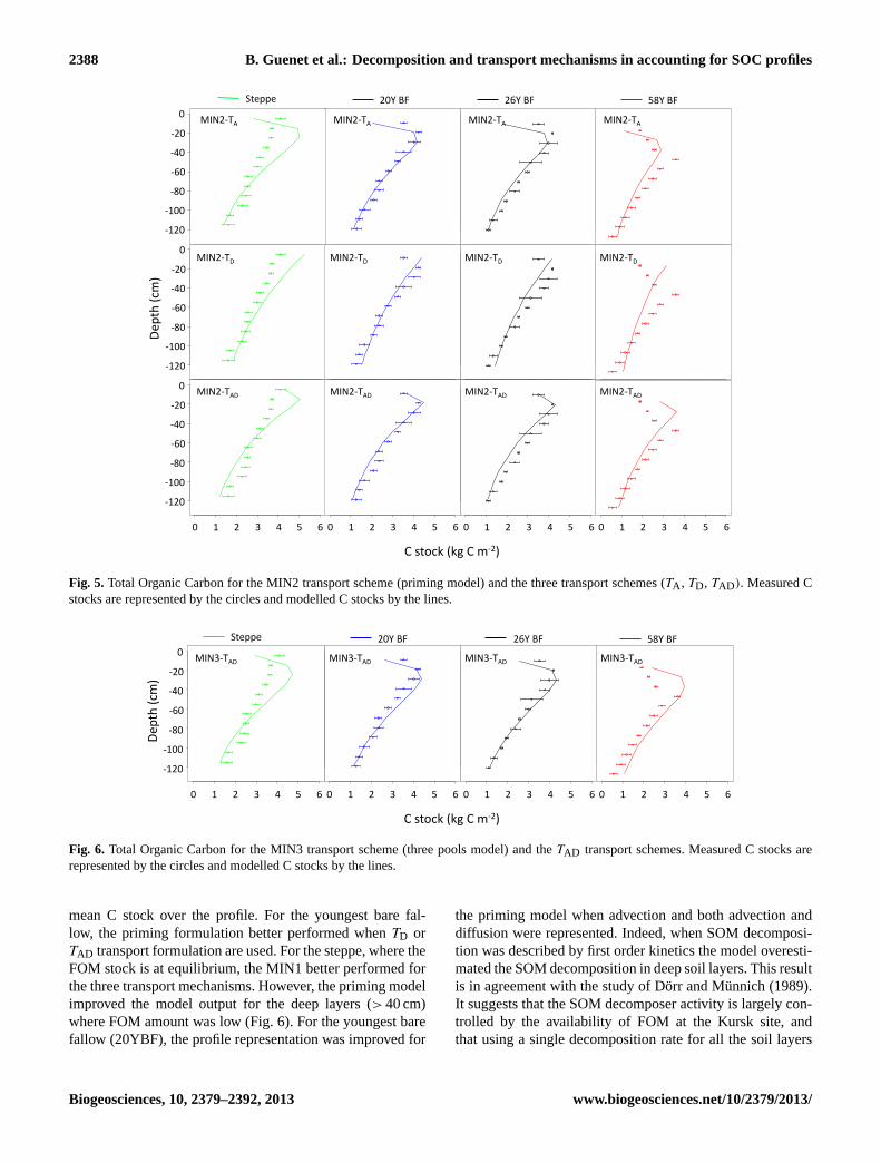
For the youngest bare fallow plots, we always observed thesame patterns. MSD values are reduced using priming model(MIN2) when soil C transport is represented using advec-tion (TA) and both advection and diffusion (TAD). The BICis following the same pattern (Table 3). In these cases, the im-provement is mainly due to an important reduction of the SBvalues indicating the priming model (MIN2) better representthe mean C stock over the profile. Indeed, the Figs. 4 and 5show that the MIN1 formulation overestimates the decompo-sition. However, when transport was represented using onlyadvection (TA) the priming model (MIN2) over estimated thedecomposition in the surface layers. The MIN3 formulation(three C pools) never presented the lowest MSD values whenboth advection and diffusion were represented. However, theSB value was reduced when SOM decomposition was de-scribed using MIN3.
For the oldest bare fallow, the priming model (MIN2) re-duced MSD values when C transport was described usingadvection only (TA) or diffusion only (TD). When C trans-port mechanism was only advection, priming model (MIN2)reduced the LC value but increased the SB value indicatingthat MIN2 better reproduced the shape of the data, but poorlyrepresented the mean C stock over the profile. ForTD for-mulation, the priming model (MIN2) better represented themean C stock over the profile (reduced SB values) and thedata scattering (reduced NU values). However, the lowestBIC values were always obtained with MIN1 whatever theC transport mechanisms used (Table 3). The highest MSDvalue was obtained with the MIN3 formulation for the oldestbare fallow, but LC value was largely reduced indicating thatsuch formulation better represented the shape of the data.
For the steppe profile, the priming model (MIN2) in-creased the MSD and the BIC values for the three transportmechanisms. In particular, when only diffusion was repre-sented (TD) the MIN2 formulation overestimated the C stock(Figs. 4 and 5). The MIN3 formulation never improved thedescription of the steppe profile.
Biogeosciences, 10, 2379–2392, 2013 www.biogeosciences.net/10/2379/2013/

B. Guenet et al.: Decomposition and transport mechanisms in accounting for SOC profiles 2387
0 1 2 3 4 5 6
-120
-100
-80
-60
-40
-20
0
0 1 2 3 4 5 6
-120
-100
-80
-60
-40
-20
0
0 1 2 3 4 5 6
-120
-100
-80
-60
-40
-20
0
0 1 2 3 4 5 6
-120
-100
-80
-60
-40
-20
0
0 1 2 3 4 5 6
-120
-100
-80
-60
-40
-20
0
0 1 2 3 4 5 6
-120
-100
-80
-60
-40
-20
0
0 1 2 3 4 5 6
-120
-100
-80
-60
-40
-20
0
0 1 2 3 4 5 6
-120
-100
-80
-60
-40
-20
0
0 1 2 3 4 5 6
-120
-100
-80
-60
-40
-20
0
0 1 2 3 4 5 6
-120
-100
-80
-60
-40
-20
0
0 1 2 3 4 5 6
-120
-100
-80
-60
-40
-20
0
0 1 2 3 4 5 6
-120
-100
-80
-60
-40
-20
0
0 1 2 3 4 5 6 0 1 2 3 4 5 6 0 1 2 3 4 5 6 0 1 2 3 4 5 6
C stock (kg C m-‐2)
0
-‐20
-‐40
-‐60
-‐80
-‐100
-‐120
0
-‐20
-‐40
-‐60
-‐80
-‐100
-‐120
0
-‐20
-‐40
-‐60
-‐80
-‐100
-‐120
Dep
th (cm)
Steppe 20Y BF 26Y BF 58Y BF
MIN1-‐TA MIN1-‐TA MIN1-‐TA MIN1-‐TA
MIN1-‐TD MIN1-‐TD MIN1-‐TD MIN1-‐TD
MIN1-‐TAD MIN1-‐TAD MIN1-‐TAD MIN1-‐TAD
Fig. 4. Total Organic Carbon for the MIN1 transport scheme (first order kinetics) and the three transport schemes (TA , TD, TAD). MeasuredC stocks are represented by the circles and modelled C stocks by the lines.
3.2 The transport formulation
Considering the entire dataset, for each SOM mineralisationformulation, the best fit was always obtained with the sametransport formulation (TAD). This was also the case for the58YBF, but for this profile, the best fit was always obtainedwith advection only. It is interesting to note that for the steppeand the youngest bare fallows (20YBF and 26YBF), thetransport mechanisms that reduce the MSD and the BIC val-ues depended on the SOM mineralisation formulation used.When using the MIN2 substrates interactions representation,the best fits were obtained with the formalisms including ad-vection and diffusion (Fig. 3). In this case, for the steppe,the SB values were particularly reduced. However, the low-est BIC values were obtained when only diffusion is repre-sented. For the 20YBF, it was the LC value that was reduced,suggesting that the shape of the curves is better representedwith advection and diffusion. When using MIN1, the best fitfor the steppe was obtained using only diffusion. The scatter-ing of the data was better represented in this case (reducedNU values). For the 20YBF, the best fit was obtained usingadvection only (TA). Here, the SB values were largely re-duced. It is interesting to note that the mechanisms transportthat produced the best fit with the data changed depending
on the FOM availability. Indeed, when SOM mineralisationwas represented by MIN1, the best fit was obtained with dif-fusion (TD) for the steppe and then with advection (TA) forthe bare fallows. With the priming model (MIN2), the low-est BIC values were always obtained with only diffusion forthe steppe, then with both advection and diffusion (TAD) for20YBF and 26YBF. Finally, for the 58YBF only advectionwas needed to fit the data.
4 Discussion
4.1 The representation of SOM decomposition
Our goal was to better separate the role of vertical transportmechanisms such as diffusion/advection given different for-mulation of SOM decomposition using a simple conceptualmodel of SOM decomposition. For the data we used, we firstshowed that the substrates interactions representation pro-posed by Wutlzer and Reichstein (2008) was an interestingformulation to represent cases where FOM is not at the equi-librium such as in the young bare fallow soil (20YBF and26YBF). For the entire set of cases, the priming model re-duced the standard bias and, therefore, better reproduced the
www.biogeosciences.net/10/2379/2013/ Biogeosciences, 10, 2379–2392, 2013
2388 B. Guenet et al.: Decomposition and transport mechanisms in accounting for SOC profiles
C stock (kg C m-‐2)
Dep
th (cm)
0 1 2 3 4 5 6
-120
-100
-80
-60
-40
-20
0
0 1 2 3 4 5 6
-120
-100
-80
-60
-40
-20
0
0 1 2 3 4 5 6
-120
-100
-80
-60
-40
-20
0
0 1 2 3 4 5 6
-120
-100
-80
-60
-40
-20
0
0 1 2 3 4 5 6
-120
-100
-80
-60
-40
-20
0
0 1 2 3 4 5 6
-120
-100
-80
-60
-40
-20
0
0 1 2 3 4 5 6
-120
-100
-80
-60
-40
-20
0
0 1 2 3 4 5 6
-120
-100
-80
-60
-40
-20
0
0 1 2 3 4 5 6
-120
-100
-80
-60
-40
-20
0
0 1 2 3 4 5 6
-120
-100
-80
-60
-40
-20
0
0 1 2 3 4 5 6
-120
-100
-80
-60
-40
-20
0
0 1 2 3 4 5 6
-120
-100
-80
-60
-40
-20
00
-‐20
-‐40
-‐60
-‐80
-‐100
-‐120
0
-‐20
-‐40
-‐60
-‐80
-‐100
-‐120
0
-‐20
-‐40
-‐60
-‐80
-‐100
-‐120
0 1 2 3 4 5 6 0 1 2 3 4 5 6 0 1 2 3 4 5 6 0 1 2 3 4 5 6
Steppe 20Y BF 26Y BF 58Y BF
MIN2-‐TA MIN2-‐TA MIN2-‐TA MIN2-‐TA
MIN2-‐TD MIN2-‐TD MIN2-‐TD MIN2-‐TD
MIN2-‐TAD MIN2-‐TAD MIN2-‐TAD MIN2-‐TAD
Fig. 5. Total Organic Carbon for the MIN2 transport scheme (priming model) and the three transport schemes (TA , TD, TAD). Measured Cstocks are represented by the circles and modelled C stocks by the lines.
!"#$%&'"(')"!"*+,-"
./0
$1"(&*-"
0 1 2 3 4 5 6
-120
-100
-80
-60
-40
-20
0
0 1 2 3 4 5 6
-120
-100
-80
-60
-40
-20
0
0 1 2 3 4 5 6
-120
-100
-80
-60
-40
-20
0
0 1 2 3 4 5 6
-120
-100
-80
-60
-40
-20
02"
+,2"
+32"
+42"
+52"
+622"
+6,2"
2" 6" ," 7" 3" 8" 4" 2" 6" ," 7" 3" 8" 4" 2" 6" ," 7" 3" 8" 4" 2" 6" ," 7" 3" 8" 4"
9$/00/" ,2:";<" ,4:";<" 85:";<"
=>?7+@A." =>?7+@A." =>?7+@A." =>?7+@A."
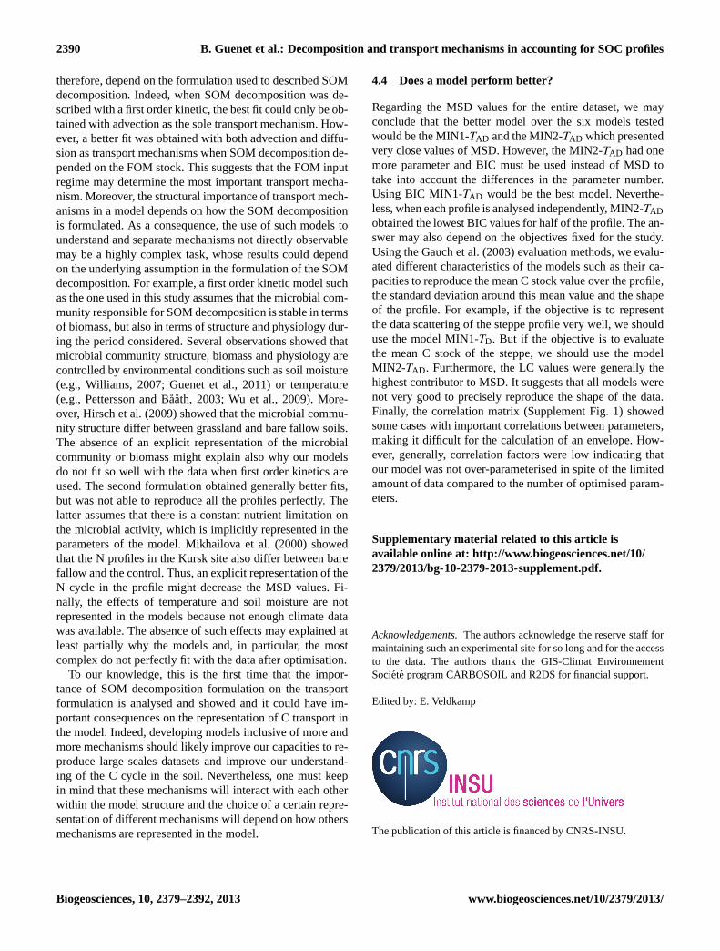
Fig. 6. Total Organic Carbon for the MIN3 transport scheme (three pools model) and theTAD transport schemes. Measured C stocks arerepresented by the circles and modelled C stocks by the lines.
mean C stock over the profile. For the youngest bare fal-low, the priming formulation better performed whenTD orTAD transport formulation are used. For the steppe, where theFOM stock is at equilibrium, the MIN1 better performed forthe three transport mechanisms. However, the priming modelimproved the model output for the deep layers (> 40 cm)where FOM amount was low (Fig. 6). For the youngest barefallow (20YBF), the profile representation was improved for
the priming model when advection and both advection anddiffusion were represented. Indeed, when SOM decomposi-tion was described by first order kinetics the model overesti-mated the SOM decomposition in deep soil layers. This resultis in agreement with the study of Dorr and Munnich (1989).It suggests that the SOM decomposer activity is largely con-trolled by the availability of FOM at the Kursk site, andthat using a single decomposition rate for all the soil layers
Biogeosciences, 10, 2379–2392, 2013 www.biogeosciences.net/10/2379/2013/

B. Guenet et al.: Decomposition and transport mechanisms in accounting for SOC profiles 2389
S58YBF20YBF26YBF
0.0 0.2 0.4 0.6 0.8 1.0 1.2
-120
-100
-80
-60
-40
-20
0
Dep
th (c
m)
C input (tC ha−1)
Fig. 7. Fresh organic matter for the four profiles calculated by themodel. The steppe, the 20YBF, the 26YBF and the 58YBF are rep-resented by the green line, the blue line, the black line and the redline, respectively. All the models share the same input scheme. Weassume that in the models a fraction of the SOM decomposed maybe as labile as the FOM and is, therefore, incorporated to the FOMpool.
parameterised on the top layers might lead to largely over-estimate SOM decomposition at depth (and underestimate itnear the surface). This conclusion is in agreement with theresults of Fontaine et al. (2007) who observed an importantincrease of SOM mineralisation at depth when FOM wasadded in an in vitro experiment. Finally, the MIN3 formula-tion never obtained the lowest BIC, suggesting that the bestfit is not always obtained with the most parameterised model.It shows that when the priming model improves the fit withthe data, it is not just an effect of increasing the number ofparameters.
4.2 Transport mechanisms
We found that for the MIN1 formulation the worst fit to thedata was always observed when only diffusion was repre-sented, except for the steppe. In particular, the LC valueswere higher indicating that the shape of the data curves wasnot well represented when using only diffusion. When theMIN2 (priming model) was used, the worst fit was alwaysobtained with advection except for 58YBF. In this case, theLC values are high, indicating that using advection only wasnot sufficient to reproduce the shape of the profile. The ad-vection rates obtained after optimisation in this study wereten times higher than those presented in Bruun et al. (2007),but ten times lower than those presented in Braakhekke etal. (2011). For the diffusion coefficient, the values obtained
here after optimisation are also higher than those of Bruunet al. (2007) (one or two range of magnitude), but this diffu-sion coefficient is a function of the bulk density (Braakhekkeet al., 2011). Thus, differences in the bulk density betweenthe soil used here and the one used by Bruun et al. (2007)might explain the different diffusion coefficients. Baisden etal. (2002) obtained good agreement between data and modeloutput with a model which only uses advection as transportmechanism. The advection rates in our study are in agree-ment with those observed by Baisden et al. (2002).
When substrates interactions are included in any of theconceptual models, we observed that only diffusion mustbe represented to properly fit the data for the steppe whereFOM is available. Then, for 20YBF and 26YBF profiles, arepresentation of diffusion and advection was needed to fitwell with the data. Finally, for the 58YBF profile, only ad-vection was needed. A shift from diffusion to advection, asthe most important mechanism to fit the data, was also ob-served when SOM mineralisation was described by first or-der kinetics. However, in this case advection was already themost important mechanism for 20YBF and 26YBF soils. Inlong-term bare fallows older than 40 yr, most of the labile Chas been mineralised (Barre et al., 2010). Consequently, theSOM in this soil is quite different in decomposability fromthat in the youngest bare fallow plots and from the steppe. Forexample, particulate organic matter, i.e., decomposing plantresidues, which are labile components of SOM are depletedfrom a temperate bare fallow in a few decades (Vasilyeva etal., 2013). Diffusion is often used to account for transportof plant debris and particulate organic matter by soil fauna,whereas advection is used to represent C transport with theliquid phase (O’Brien and Stout, 1978; Wynn et al., 2005;Braakhekke et al., 2011). Soil fauna activity is closely re-lated to SOM availability (Decaens, 2010). Therefore, theimportance of soil fauna in the transport C in our sites de-creased when FOM input were stopped and, therefore, whenSOM availability was reduced. This suggests that differentpools of SOM could be transported through different mech-anisms. The more labile OM may be transported mainly bybioturbation, whereas the more stabilised may be transportedwith the liquid phase. To our knowledge, this is the first timethat different transport mechanisms are suggested for differ-ent pools of C. This assumption must be tested against othersoil profiles from bare fallow experiments, but if confirmed itsuggests that soil models using different pools of C and aim-ing to represent the C distribution within a profile must usedifferent transport mechanisms for labile and stable pools.
4.3 Transport mechanisms depending on the SOMdecomposition formulation
We observed that the transport mechanism inducing thebest fit for youngest bare fallow (20YBF and 26YBF)where FOM stock are out from equilibrium was not alwaysthe same for each decomposition formulation and might,
www.biogeosciences.net/10/2379/2013/ Biogeosciences, 10, 2379–2392, 2013
2390 B. Guenet et al.: Decomposition and transport mechanisms in accounting for SOC profiles
therefore, depend on the formulation used to described SOMdecomposition. Indeed, when SOM decomposition was de-scribed with a first order kinetic, the best fit could only be ob-tained with advection as the sole transport mechanism. How-ever, a better fit was obtained with both advection and diffu-sion as transport mechanisms when SOM decomposition de-pended on the FOM stock. This suggests that the FOM inputregime may determine the most important transport mecha-nism. Moreover, the structural importance of transport mech-anisms in a model depends on how the SOM decompositionis formulated. As a consequence, the use of such models tounderstand and separate mechanisms not directly observablemay be a highly complex task, whose results could dependon the underlying assumption in the formulation of the SOMdecomposition. For example, a first order kinetic model suchas the one used in this study assumes that the microbial com-munity responsible for SOM decomposition is stable in termsof biomass, but also in terms of structure and physiology dur-ing the period considered. Several observations showed thatmicrobial community structure, biomass and physiology arecontrolled by environmental conditions such as soil moisture(e.g., Williams, 2007; Guenet et al., 2011) or temperature(e.g., Pettersson and Baath, 2003; Wu et al., 2009). More-over, Hirsch et al. (2009) showed that the microbial commu-nity structure differ between grassland and bare fallow soils.The absence of an explicit representation of the microbialcommunity or biomass might explain also why our modelsdo not fit so well with the data when first order kinetics areused. The second formulation obtained generally better fits,but was not able to reproduce all the profiles perfectly. Thelatter assumes that there is a constant nutrient limitation onthe microbial activity, which is implicitly represented in theparameters of the model. Mikhailova et al. (2000) showedthat the N profiles in the Kursk site also differ between barefallow and the control. Thus, an explicit representation of theN cycle in the profile might decrease the MSD values. Fi-nally, the effects of temperature and soil moisture are notrepresented in the models because not enough climate datawas available. The absence of such effects may explained atleast partially why the models and, in particular, the mostcomplex do not perfectly fit with the data after optimisation.
To our knowledge, this is the first time that the impor-tance of SOM decomposition formulation on the transportformulation is analysed and showed and it could have im-portant consequences on the representation of C transport inthe model. Indeed, developing models inclusive of more andmore mechanisms should likely improve our capacities to re-produce large scales datasets and improve our understand-ing of the C cycle in the soil. Nevertheless, one must keepin mind that these mechanisms will interact with each otherwithin the model structure and the choice of a certain repre-sentation of different mechanisms will depend on how othersmechanisms are represented in the model.
4.4 Does a model perform better?
Regarding the MSD values for the entire dataset, we mayconclude that the better model over the six models testedwould be the MIN1-TAD and the MIN2-TAD which presentedvery close values of MSD. However, the MIN2-TAD had onemore parameter and BIC must be used instead of MSD totake into account the differences in the parameter number.Using BIC MIN1-TAD would be the best model. Neverthe-less, when each profile is analysed independently, MIN2-TADobtained the lowest BIC values for half of the profile. The an-swer may also depend on the objectives fixed for the study.Using the Gauch et al. (2003) evaluation methods, we evalu-ated different characteristics of the models such as their ca-pacities to reproduce the mean C stock value over the profile,the standard deviation around this mean value and the shapeof the profile. For example, if the objective is to representthe data scattering of the steppe profile very well, we shoulduse the model MIN1-TD. But if the objective is to evaluatethe mean C stock of the steppe, we should use the modelMIN2-TAD . Furthermore, the LC values were generally thehighest contributor to MSD. It suggests that all models werenot very good to precisely reproduce the shape of the data.Finally, the correlation matrix (Supplement Fig. 1) showedsome cases with important correlations between parameters,making it difficult for the calculation of an envelope. How-ever, generally, correlation factors were low indicating thatour model was not over-parameterised in spite of the limitedamount of data compared to the number of optimised param-eters.
Supplementary material related to this article isavailable online at:http://www.biogeosciences.net/10/2379/2013/bg-10-2379-2013-supplement.pdf.
Acknowledgements.The authors acknowledge the reserve staff formaintaining such an experimental site for so long and for the accessto the data. The authors thank the GIS-Climat EnvironnementSociete program CARBOSOIL and R2DS for financial support.
Edited by: E. Veldkamp
The publication of this article is financed by CNRS-INSU.
Biogeosciences, 10, 2379–2392, 2013 www.biogeosciences.net/10/2379/2013/
B. Guenet et al.: Decomposition and transport mechanisms in accounting for SOC profiles 2391
References
Afanasyeva, E. A.: Chernozemy sredne-russkoi vozvishennosti,Nauka, Moscow, 224 pp., 1966 (in Russian).
Baisden, W. T.: A multiisotope C and N modeling analysis of soilorganic matter turnover and transport as a function of soil depthin a California annual grassland soil chronosequence, GlobalBiogeochem. Cy., 16, 1135,doi:10.1029/2001GB001823, 2002.
Barre, P., Eglin, T., Christensen, B. T., Ciais, P., Houot, S., Katterer,T., van Oort, F., Peylin, P., Poulton, P. R., Romanenkov, V., andChenu, C.: Quantifying and isolating stable soil organic car-bon using long-term bare fallow experiments, Biogeosciences,7, 3839–3850,doi:10.5194/bg-7-3839-2010, 2010.
Batjes, N. H.: Total carbon and nitrogen in the soils of the world,Eur. J. Soil Sci., 47, 151–163, 1996.
Braakhekke, M. C., Beer, C., Hoosbeek, M. R., Reichstein, M.,Kruijt, B., Schrumpf, M., and Kabat, P.: SOMPROF: A verticallyexplicit soil organic matter model, Ecol. Model., 222, 1712–1730, 2011.
Bruun, S., Christensen, B. T., Thomsen, I. K., Jensen, E. S., andJensen, L. S.: Modeling vertical movement of organic matter ina soil incubated for 41 years with14C labeled straw, Soil Biol.Biochem., 39, 368–371, 2007.
Coleman, K., Jenkinson, D. S., Crocker, G. J., Grace, P. R., Klir,J., Korschens, M., Poulton, P. R., and Richter, D. D.: Simulat-ing trends in soil organic carbon in long-term experiments usingRothC-26.3., Geoderma, 81, 29–44, 1997.
Decaens, T.: Macroecological patterns in soil communities, Glob.Ecol. Biogeogr., 19, 287–302, 2010.
Dorr, H. and Munnich, K.: Downward movement of soil organicmatter and its influence on trace element transport, Radiocarbon,31, 655–663, 1989.
Elzein, A. and Balesdent, J.: Mechanistic Simulation of Vertical-Distribution of Carbon Concentrations and Residence Times inSoils, Soil Sci. Soc. Am. J., 59, 1328–1335, 1995.
Feng, X., Peterson, J. C., Quideau, S. A., Virginia, R. A., Graham,R. C., Sonder, L. J., and Chadwick, O. A.: Distribution, accumu-lation, and fluxes of soil carbon in four monoculture lysimetersat San Dimas Experimental Forest, California, Geochim. Cos-mochim. Ac., 63, 1319–1333, 1999.
Fontaine, S. and Barot, S.: Size and functional diversity of microbepopulations control plant persistence and long-term soil carbonaccumulation, Ecol. Lett., 8, 1075–1087, 2005.
Fontaine, S., Barot, S., Barre, P., Bdioui, N., Mary, B., and Rumpel,C.: Stability of organic carbon in deep soil layers controlled byfresh carbon supply, Nature, 450, 277–280, 2007.
Friedlingstein, P., Cox, P., Betts, R., Bopp, L., Von Bloh, W.,Brovkin, V., Cadule, P., Doney, S., Eby, M., Fung, I., Bala, G.,John, J., Jones, C., Joos, F., Kato, T., Kawamiya, M., Knorr, W.,Lindsay, K., Matthews, H. D., Raddatz, T., Rayner, P., Reick,C., Roeckner, E., Schnitzler, K. G., Schnur, R., Strassmann, K.,Weaver, A. J., Yoshikawa, C., and Zeng, N.: Climate-carbon cy-cle feedback analysis: Results from the C4MIP model intercom-parison, J. Climate 19, 3337–3353, 2006.
Gauch Jr., H. G., Hwang, J. T., and Fick, G. W.: Model Evaluationby Comparison of Model-Based Predictions and Measured Val-ues, Agron. J., 95, 1442–1446, 2003.
Guenet, B., Lenhart, K., Leloup, J., Giusti-Miller, S., Pouteau, V.,Mora, P., Nunan, N., and Abbadie, L.: The impact of long-termCO2 enrichment and moisture levels on soil microbial commu-
nity structure and enzyme activities, Geoderma, 170, 331–336,2011.
Hirsch, P. R., Gilliam, L. M., Sohi, S. P., Williams, J. K., Clark, I.M., and Murray, P. J.: Starving the soil of plant input for 50 yearsreduces abundance but not diversity of soil bacterial communi-ties, Soil Biol. Biochem., 41, 2021–2024, 2009.
Jenkinson, D. S. and Coleman, K.: The turnover of organic carbonin subsoils. Part 2. Modelling carbon turnover, Eur. J. Soil Sci.,59, 400–413, 2008.
Jobbagy, E. G. and Jackson, R. B.: The vertical distribution of soilorganic carbon and its relation to climate and vegetation, Ecol.Appl., 10, 423–436, 2000.
Kobayashi, K. S. and Salam, M. U.: Comparing simulated and mea-sured values using mean squared deviation and its components.Agron. J., 92, 345–352, 2000.
Lueken H., Hutcheon, W. L., and Paul, E. A.: The influence of ni-trogen on the decomposition of crop residues in soil, Can. J. ofSoil Sci., 42, 276–288, 1962.
Manzoni, S. and Porporato, A.: Soil carbon and nitrogen mineral-isation: Theory and models across scales, Soil Biol. Biochem.,41, 1355–1379, 2009.
MEA: Millennium Ecosystem Assessment-Nutrient Cycling, WorldResource Institute, Washington DC, 2005.
Mikhailova, E. A., Vassenev, R. B., Schwager, I. I., and Post, S. J.:Cultivation effects on soil carbon and nitrogen contents at depthin the Russian Chernozem, Soil Sci. Soc. Am. J., 64, 738–745,2000
O’Brien, B. J. and Stout, J. D.: Movement and turnover of soil or-ganic matter as indicated by carbon isotope measurements, SoilBiol. Biochem., 10, 309–317, 1977.
Parton, W. J., Stewart, J. W. B., and Cole, C. V.: Dynamics of C, N,P and S in grassland soils – a model, Biogeochemistry, 5, 109–131, 1988.
Pettersson, M. and Baath, E.: Temperature-dependent changes inthe soil bacterial community in limed and unlimed soil, FEMSMicrobiol. Ecol., 45, 13–21, 2003.
R Development Core Team: A language and environment for statis-tical computing, R Foundation for Statistical Computing, Vienna,Austria, ISBN 3-900051-07-0,http://www.R-project.org., 2010.
Rumpel, C. and Kogel-Knabner, I.: Deep soil organic matter – akey but poorly understood component of terrestrial C cycle, PlantSoil, 338, 143–158, 2010.
Salome, C., Nunan, N., Pouteau, V., Lerch, T. Z., and Chenu, C.:Carbon dynamics in topsoil and in subsoil may be controlled bydifferent regulatory mechanisms, Glob. Change Biol., 16, 416–426, 2010.
Sanaullah, M., Chabbi, A., Leifeld, J., Bardoux, G., Billou, D., andRumpel, C.: Decomposition and stabilization of root litter in top-and subsoil horizons: what is the difference?, Plant Soil, 338,127–141, 2010.
Santaren, D., Peylin, P., Viovy, N., and Ciais, P.: Optimizinga process-based ecosystem model with eddy-covariance fluxmeasurements: A pine forest in southern France, Global Bio-geochem. Cy., 21, GB2013,doi:10.1029/2006GB002834, 2007.
Schimel, D. S.: Terrestrial ecosystems and the carbon cycle, Glob.Change Biol., 1, 77–91, 1995.
Schlesinger, H. W.: Evidence from chronosequence studies for alow carbon-storage potential of soils, Nature, 348, 232–234,1990.
www.biogeosciences.net/10/2379/2013/ Biogeosciences, 10, 2379–2392, 2013
2392 B. Guenet et al.: Decomposition and transport mechanisms in accounting for SOC profiles
Soetaert, K., Petzoldt, T., and Setzer, R. W.: Solving DifferentialEquations in R: Package deSolve, J. Stat. Softw., 33, 1–25, 2010.
Sparling, G. S., Cheschire, M. V., and Mundie, C. M.: Effect ofbarley plants on the decomposition of 14C-labelled soil organicmatter, J. Soil Sci., 33, 89–100, 1982.
Sugden, A., Stone, R., and Ash, C.: Ecology in the underworld –Introduction, Science, 304, 1613–1613, 2004.
Tarantola, A.: Inverse Problem Theory: Methods of Data Fittingand Model Parameter Estimation, Elsevier Science Ltd., 630 pp.,1987.
Tarnocai, C., Canadell, J. G., Schuur, E. A. G., Kuhry, P., Mazhi-tova, G., and Zimov, S.: Soil organic carbon pools in the north-ern circum-polar permafrost region, Global Biogeochem. Cy.,23, GB2023,doi:10.1029/2008GB003327, 2009.
Vasilyeva, N. A., Chenu, C., Tyugai, Z. N., and Milanovskiy, E. Y.:Century scale C metastability in full Chernozem profiles underchanged organic matter input and tillage, in press, 2013.
Vinogradov, B. V.: Aerospace studies of protected natural areas inthe USSR, in: Conservation, science and society, Nat. Resour.Res., XXI, Vol. 2, 435–448, UNESCO-UNEP, Paris, 1984.
Williams, M.: Response of microbial communities to water stressin irrigated and drought-prone tallgrass prairie soils, Soil Biol.Biochem., 39, 2750–2757, 2007.
Wu, J., Brookes, P. C., and Jenkinson, D. S.: Formation and destruc-tion of microbial biomass during the decomposition of glucoseand Ryegrass in Soil, Soil Biol. Biochem., 25, 1435–1441, 1993.
Wu, Y., Xiongsheng, Y., Haizhen, W., Na, D., and Jianming,X.: Does history matter? Temperature effects on soil microbialbiomass and community structure based on the phospholipidfatty acid (PLFA) analysis, J. Soil Sediment, 10, 223–230, 2009.
Wutzler, T. and Reichstein, M.: Colimitation of decomposition bysubstrate and decomposers – a comparison of model formula-tions, Biogeosciences, 5, 749–759,doi:10.5194/bg-5-749-2008,2008.
Wynn, J. G., Bird, M. I., and Wong, V. N. L.: Rayleigh distillationand the depth profile of 13C/12C ratios of soil organic carbonfrom soils of disparate texture in Iron Range National Park, FarNorth Queensland, Australia, Geochim. Cosmochim. Ac., 69,1961–1973, 2005.
Zhu, C., Byrd, R. H., Lu, P., and Nocedal, J.: A limited memoryalgorithm for bound constrained optimisation, SIAM J. Sci. Stat.Comput., 16, 1190–1208, 1995.
Biogeosciences, 10, 2379–2392, 2013 www.biogeosciences.net/10/2379/2013/