Opec 12048 rev2

Stochastic volatility models for the Brent oilfutures market: forecasting and extractingconditional moments

Per Bjarte Solibakke

Professor, Molde University College, Britveien 2, Kvam, 6402 Molde, Norway. Email:[email protected]

Abstract

This paper builds and implements a multifactor stochastic volatility model for the latent (andobservable) volatility from the front month future contracts at the Intercontinental CommodityExchange (ICE), London, applying Bayesian Markov chain Monte Carlo simulation methodologiesfor estimation, inference and model adequacy assessment. Stochastic volatility is the main way time-varying volatility is modelled in financial markets. An appropriate scientific model description,specifying volatility as having its own stochastic process, broadens the applications into derivativepricing purposes, risk assessment and asset allocation and portfolio management. From an estimatedoptimal and appropriate stochastic volatility model, the paper reports risk and portfolio measures,extracts conditional one-step-ahead moments (smoothing), forecasts one-step-ahead conditionalvolatility (filtering), evaluates shocks from conditional variance functions, analyses multistep-aheaddynamics and calculates conditional persistence measures. (Exotic) option prices can be calculatedusing the re-projected conditional volatility. Observed market prices and implied volatilities estab-lish market risk premiums. The analysis adds insight and enables forecasts to be made, building upthe methodology for developing valid scientific commodity market models.

1. Introduction

This paper builds and assesses scientific stochastic volatility (SV) models for the Brentoil futures markets and traded at Intercontinental Commodities Exchange (ICE),London.1 Knowledge of the empirical properties of the Brent oil future prices is importantwhen constructing risk-assessment and management strategies. Energy market partici-pants who understand the dynamic behaviour of forward prices are more likely to haverealistic expectations about future prices and the risks to which they are exposed. Time-varying volatility is endemic in financial markets. Such risks may change through time incomplicated ways, and it is natural to build stochastic models for the temporal evolution

Classification: C11, C63, G17, G32

1

© 2015 Organization of the Petroleum Exporting Countries. Published by John Wiley & Sons Ltd, 9600 Garsington

Road, Oxford OX4 2DQ, UK and 350 Main Street, Malden, MA 02148, USA.

in volatility. One of the main objectives of the paper is therefore to structure a scientificmodel specifying volatility as having its own stochastic process, appropriately describingthe evolution of the market volatility. The implementation adapts the Markov ChainMonte Carlo (MCMC) estimator proposed by Chernozhukov and Hong (2003), claimedto be substantially superior to conventional derivative-based hill climbing optimisers forthis stochastic class of problems. Moreover, under correct specification of the structuralmodel the normalised value of the objective function is asymptotically χ2 distributed (andthe degrees of freedom is well specified). An appropriate and well-specified SV model forthe ICE markets broaden applications into derivative pricing purposes, risk assessmentand management, asset allocation and portfolio management. The main objective of thepaper was therefore to prepare the foundation for methodologies comprising derivativepricing, implied volatilities for risk premium calculations, asset allocations and riskmanagement.

Stochastic volatility models have an intuitive and simple structure and can explain themajor stylised facts of asset, currency and commodity returns. The volatility of future oilprices are of interest for many reasons. Firstly, energy price volatility could hinder invest-ments in new and advanced technology and equipment. Secondly, if oil prices and otherenergy prices are cointegrated, a volatile market might make it harder for consumers andbusinesses to predict their raw-material costs.2 In a booming economy, an increase inprices may make it harder for economic growth to occur. In general, energy prices moverelatively slowly when conditions are calm, while they move faster when there is morenews, uncertainty and trading. One of the most prominent stylised fact of returns on finan-cial assets is that their volatility changes over time. As the most important determinant ofthe price of an option is the uncertainty associated with the price of the underlying asset,volatility is of paramount importance in financial analysis. Risk managers are particularlyinterested in measuring and predicting volatility, as higher levels imply a higher chance oflarge adverse price changes. For energy markets like other markets, the motivation for SVis the observed non-constant and frequently changing volatility.The SV implementation isan attempt to specify how the volatility changes over time. Bearing in mind that volatilityis a non-traded instrument, which suggests imperfect estimates, the volatility can be inter-preted as a latent variable that can be modelled and predicted through its direct influenceon the magnitude of returns. Besides, as the ICE commodity market writes options on thefront month future contracts, SV models are also motivated by the natural pricing of theseoptions, when over time volatility change. Finally, for energy markets observed returnsand volatility changes seem so frequent that it is appropriate to model both returns andvolatility by random variables.

The paper focuses on the Bayesian MCMC modelling strategy used by Gallant andTauchen (2010a, 2010b) and Gallant and McCulloch (2011)3 implementing uni- andmultivariate statistical models derived from scientific considerations. The method is a

Per Bjarte Solibakke2

OPEC Energy Review •• 2015 © 2015 Organization of the Petroleum Exporting Countries

systematic approach to generate moment conditions for the generalised method ofmoments (GMM) estimator (Hansen, 1982) of the parameters of a structural model.Moreover, the implemented Chernozhukov and Hong (2003) estimator keeps modelparameters in the region where predicted shares are positive for every observed price/expenditure vector. For conventional derivative-based hill-climbing algorithms, this isnearly impossible to achieve. Moreover, the methodology supports restrictions, inequal-ity restrictions and informative prior information (on model parameters and functionalsof the model). Asset pricing models as the habit persistence model of Campbell andCochrane (1999), the long-run risk model of Bansal and Yaron (2004) and the prospecttheory model of Barberis et al. (2001) are all implemented. For the SV model implemen-tation, the enhanced statistical and scientific stochastic model calibration methodologiescan greatly enhance portfolio management, elaborate and extend the decomposition andaggregation of overall corporate and institutional risk assessment and management. Infact, appropriate MCMC-estimated SV model simulations can generate probability dis-tributions for the calculation of value at risk (VaR/CVaR) and Greek letters for portfoliorebalancing and model parameters can be the basis for forecasting the mean and volatil-ity for forward assessment of risk, portfolio management and other derivative pricingpurposes. However, on the downside, as volatility is latent (and unobservable) coincidingwith the fact that the conditional variances are complex functions complicating themaximum likelihood, estimations will be imperfect and a single optimal estimation tech-nique is probably not available.

It is simple to make forecasts using the MCMC framework. Hence, both the mean andvolatility are able to be forecasted adding content to future contract prices. Moreover, there-projection method (Gallant and Tauchen, 1998) based on long simulated data series canextend projections. The post-estimation analysis can be used as a general-purpose tech-nique for characterising the dynamic response of the partially observed system to itsobservable history. Forecasting the conditional moments and the use of filtered volatility(with a purelyARCH-type meaning) and multistep-ahead dynamics are some features thatreally add strength to the methodology building of scientifically valid models. Ultimately,the analysis may therefore contribute to more realistic risk methodologies for energymarkets and for market participants an improved understanding of the general stochasticbehaviour inducing more realistic expectations about future prices and the risks to whichthey are exposed. Previous research on energy market prices is extensive. Studies adoptingthe Heath–Jarrow–Morton (HJM) assuming dynamics for the forward and swap price evo-lution have been suggested. In particular, Bjerksund et al. (2000), Keppo et al. (2004),Benth and Koekebakker (2008) and Kiesel et al. (2009) have used contracts for theNASDAQ OMX and European Energy Exchange (EEX) electricity markets. The sameapproach for energy markets in general can be found in Clewlow and Strickland (2000).However, modelling the price dynamics, where the contracts delivers over a period, creates

Stochastic volatility models for the Brent oil futures market 3

OPEC Energy Review •• 2015© 2015 Organization of the Petroleum Exporting Countries

challenges that are not present in the fixed income market theory (see Musiela andRutkowski, 1997). To resolve this problem the LIBOR models in interest rate theory (seeBrigo and Mercurio, 2001) exclusively model contracts that are traded in the market anddo not have delivery periods, which cannot be decomposed into other traded contracts.Theresult is much more freedom to state reasonable stochastic dynamical models4 (Benthet al., 2008). Kiesel et al. (2009) propose a two-factor model for electricity prices. Eventhough the research on the energy market is voluminous, the LIBOR approach and model-ling different parts of the term structure individually make the SV modelling interestingfor derivative purposes, risk management and asset allocation. The contribution of ourstudy is therefore threefold.

Firstly, this paper is one of the first scientific model investigation of the behaviour ofthe front month future contracts traded at the ICE commodity exchange. In particular, itprovides the one of the first study to our knowledge that examines modelling the returnvolatility using scientific SV models together with the Bayesian estimation and inferencemethodology (MCMC). Secondly, it improves assessment methodology for the evaluationof model fit and empirical scientific content. Plotting suitable measures of location andscale of the posterior distributions assesses the scientific model. That is, plots showingsmall location changes and increasing scale is favourable for scientific well-definedmodels. Thirdly, to our knowledge this paper is unique in analysing conditional momentforecasts for energy market contracts (point estimates and densities). In particular, it inves-tigates the possibility that lagged returns contribute little if any additional informationabout future returns and variances. Fourthly, risk management (VaR/CVaR) and asset allo-cation (Greeks) measures are available for both conditional and unconditional moments.Finally, particle filtering, multistep-ahead forecast and persistence are reported for thecontracts. The rest of the paper is therefore as follows. Section 2 presents backgroundresearch and defines the data set. Section 3 describes the SV methodology. Section 4 con-ducts the GSM SV specifications and assesses model validity. Section 5 interprets themodel result. Section 6 uses the estimated model results for mean and volatility prediction,volatility filtering and describes how to extend the model assessment features of the meth-odology for option pricing and implied volatilities calculations. Section 7 summarises andconcludes.

2. Background and data set

Markets have mechanism to balance supply and demand. These physical contracts containactual consumption and production as part of the contract fulfilment. Financial marketcontracts are linked to some reference spot price, and they are settled in cash.The contractscan be considered as side bets on the physical system. The basic exchange traded contractsare written on the price at maturity. Hence, the financial swap contracts are settled in cash



against the spot price. The exchanges also offer options written on front month, quarterand front year futures/forwards. The ICE Commodity Exchange is the market for energyand related products with an international orientation. The participants on the exchangecan trade via open and cost-effective electronic access on equal terms. The energyexchange is located in London, UK. The Intercontinental Exchange (ICE) was formed todevelop a transparent marketplace for over the counter (OTC) energy markets. The ICEDerivatives Markets was started in 2000. This is an electronic order book where partici-pants can see the system orders (anonymously) and the best ask and bid prices with corre-sponding volumes. Pricing is established at the end of the opening phase5 and duringcontinuous trading. The main products traded are forward/futures and options. Similar toother international energy markets, the majority of members on the derivative market usethe market for risk management purposes.

The usual product definitions apply. The front month future contracts trade forapproximately 2/3 months. The analysis uses only the last front month contract pricessecuring trading volume, liquidity and information flow. That is, the time series is con-structed of contract prices from approximately January 10 to February 10 of the same yearof trading. All returns are calculated from prices within one contract. The daily analysescover the period from the end of 2008 until the mid of 2014 (July 4), a total of six and a halfconsecutive years and 1680 returns. The main argument for using the front month con-tracts is the fact that these contracts are the ICE markets underlying assets for active optiontrading. Any signs of successful SV-model implementations for the future market willindicate non-predictive market features and a minimum of weak-form market efficiency.Consequently, the markets are applicable for enhanced risk management activities includ-ing pricing of hedging instruments as well as conventional portfolio/fund managementprocedures. For all market participants an efficient market suggests pricing mechanismsreflecting all relevant historical information indicating a foundation of non-predictive andefficient market pricing, which are important ingredients for successful market implemen-tation. In the end only an effective market can give guarantees for market prices close tothe marginal cost of expanding capacity. It is important that participants can infer that allhedging instruments both for short and long run are fairly priced at all times.

The daily percentage change (logarithmic) of the data sets from the end of 2008 to thebeginning of July 2014 is yt, t = 1, . . . , 1680. Characteristics of the markets financiallytraded contracts are reported in Table 1. The mean is negative and the standard deviation,the maximum value and the kurtosis are relatively high. The Jarque–Bera and Quantilenormal test statistics suggest non-normal return distributions. Serial correlation in themean equation is not strong and the Ljung–Box Q-statistic (Ljung and Box, 1978) is notsignificant. Volatility clustering using the Ljung–Box test statistic (Ljung and Box, 1978)for squared returns (Q2) and ARCH statistics is significantly present. The KPSS(Kwiatowski et al., 1992) statistic cannot reject neither level nor trend (12) stationary



Tab

le1

Cha

ract

eris

tics

ofth

eB

rent

oilf

ront

mon

thfu

ture

mar

ket

Mea

n/m

ode

Med

ian

std.

dev.

Max

imum

/m

inim

umM

omen

tK

urt/

Ske

wQ

uant

ile

Kur

t/S

kew

Qua

ntil

eno

rmal

Jarq

ue–B

era

Ser

iald

epen

denc

e

Q(1

2)Q

2 (12)

−0.

0006

90.

0601

712

.706

64.

6491

90.

4028

011

.613

115

18.9

216

.781

014

02.8

00.

0000

02.

1204

1−

10.9

455

−0.

2478

6−

0.03

022

{0.0

030}

{0.0

000}

{0.1

580}

{0.0

000}

BD

S-Z

-sta

tist

ics

(ε=

1)K

PS

S(s

tati

onar

y)A

ugm

ente

dD

F-t

est

AR

CH

(12)

VaR

2.5%

/C

VaR

2.5%

m=

2m

=3

m=

4m

=5

Lev

elT

rend

11.3

582

14.3

443

16.6

329

19.2

271

0.23

737

0.11

020

−43

.041

942

0.96

3−

4.69

2{0

.000

0}{0

.000

0}{0

.000

0}{0

.000

0}{0

.276

4}{0

.107

2}{0

.000

0}{0

.000

0}−

6.71

9

The

num

bers

inbr

aces

deno

teP

-val

ues

fors

tati

stic

alsi

gnifi

canc

e.



price change series. The Dickey–Fuller test adds support to stationary series. The BDS(Brock et al., 1996) test statistics report highly significant data dependence. The pricechange (log returns) data series are shown in the upper part of Fig. 1 (together with a dis-tribution to the left). From the return plots, the series show some large returns at the begin-ning of the series6 and the level of volatility seems to change randomly. The plots togetherwith theARCH and Ljung–Box test statistics (Q2) in Table 1 manifest volatility clustering.Moreover, the QQ-plot in part (b) of Fig. 1 shows that the series distribution is morepeaked and has fatter tails than a corresponding normal distribution. For the left and theright tails of the distributions, the number of large negative price changes seems to occurmore often than large positive. However, the size of the returns is higher for positive pricechanges. That is—the series will most likely have a negative drift with larger positive thannegative price jumps. These facts together with a third moment different from zero anda fourth moment higher than three, indicates both a non-normal distribution andleptokurtosis features. Finally, for later comparisons, the value at risk (VaR) and expectedshortfall (CVaR) numbers report percentile and expected shortfall numbers for long posi-tions at less than 2.5 per cent and 0.5 per cent. For our scientific model calibrations, thesefeatures found in the commodity series suggests non-linear models, simply because linearmodels would not be able to generate these data.

3. Theoretical SV model background and motivation

Stochastic volatility models provide alternative models and methodologies to (G)ARCHmodels.7

The time-varying volatility is endemic in global financial markets. The SV approachspecifies the predictive distribution of returns indirectly, via the structure of the model,rather than directly (ARCH).The main advantage of direct volatility modelling is conveni-ence and perhaps its being more natural. Relative to ARCH the SV model therefore has itsown stochastic process without worries about the implied one-step-ahead distribution ofreturns recorded over an arbitrary time interval convenient for the econometrician. More-over, simulation strategies developed to efficiently estimate SV models have given accessto a broad range of fully parametric models. This enriched literature has brought us closerto the empirical realities of the global markets.8 However, SV and ARCH models explainthe same stylised facts and have many similarities.

The starting point is the application of Andersen et al. (2002) considering the familiar

SV diffusion for an observed stock price St given bydS

ScV dt V dWt

tt t t= +( ) +μ 1 , where

the unobserved volatility process Vt is either log linear or square root (affine) (W2t).The W1t

and W2t are standard Brownian motions that are possibly correlated with corr(dW1t,dW2t) = ρ. Andersen et al. (2002) estimate both versions of the SV model with daily



-15

-10

-5

0

5

10

15

a. Brent oil front month future contracts returns plots 2008–2014.

1008 09 11 12 13 14

Front Month

b. Brent oil front month future contracts returns: quantile–quantile plots.

-8

-6

-4

-2

0

2

4

6

8

-15 -10 -5 0 5 10 15Quantiles of FRONT_MONTH

Qua

ntile

s of

Nor

mal

Figure 1 The ICE Brent oil front month contracts: returns characteristics for the period 2008–2014.



S&P500 stock index data, from 1953 to December 31, 1996. Both SV model versions aresharply rejected. However, adding a jump component to a basic SV model improves the fitsharply, reflecting two familiar characteristics: thick non-Gaussian tails and persistenttime-varying volatility. A SV model with two SV factors show encouraging results inChernov et al. (2003). The authors consider two broad classes of setups for the volatilityindex functions and factor dynamics: an affine setup and a logarithmic setup. The modelsare estimated using daily data on the DOW Index, January 2, 1953–July 16, 1999. Theyfind that models with two volatility factors do much better than do models with only asingle volatility factor.They also find that the logarithmic two-volatility factor models out-perform affine jump diffusion models and basically provide acceptable fit to the data. Oneof the volatility factors is extremely persistent and the other strongly mean-reverting. TheSV model for the European energy market applies the logarithmic model with two SVfactors (Chernov et al., 2003). Moreover, the SV model is extended to facilitate correla-tion between the mean (W1t) and the two SV factors (W2t, W3t). The main argument for thecorrelation modelling is to introduce asymmetry effects (correlation between return inno-vations and volatility innovations).This paper formulation of a SV model for the Europeanenergy market’s price change process (yt) therefore becomes

y a a y a V V u

V b b V b u

t t t t t

t t t

= + −( ) + +( )⋅= + −( ) +

−

−

0 1 1 0 1 2 1

1 0 1 1 1 0 2

exp

,

VV c c V c u

u W

u s r W r W

u

t t t

t t

t t t

2 0 1 2 1 0 3

1 1

2 1 1 1 12

2

3

1

= + −( ) +=

= ⋅ + − ⋅( )

−,

tt

t t

sr W r r r r W

r r r r r=

⋅ + − ⋅( )( ) −( )⋅

+ − − − ⋅( )( ) −2

2 1 3 2 1 12

2

22

3 2 1 1

1

1 1 222

3( ) ⋅

⎛

⎝

⎜⎜

⎞

⎠

⎟⎟

W t

(1)

where Wit, i = 1, 2 and 3 are standard Brownian motions (random variables). The param-eter vector is ρ = (a0, a1, b0, b1, s1, c0, c1, s2, r1, r2, r3). The r’s are correlation coefficientsfrom a Cholesky decomposition;9 enforcing an internally consistent variance/covariancematrix. Early references are Rosenberg (1972), Clark (1973) and Taylor (1982) andTauchen and Pitts (1983). References that are more recent are Gallant et al. (1991, 1997),Andersen (1994), Chernov et al. (2003), Durham (2003), Shephard (2004) and Taylor(2005). The model above has three stochastic factors. Extensions to four and more factorscan be easily implemented through this model setup. Even jumps with the use of Poissondistributions for jump intensity are applicable (complicates estimations considerably). Asshown by Chernov et al. (2003) liquid financial markets make a much better model fit



introducing two SV factors. One of the volatility factors that is strongly mean reverting tofatten tails and a second factor that is extremely persistent to capture volatility clustering.

The motivations for the use of SV models are threefold. Firstly, SV models assume thevolatility at day t is partially determined by unpredictable events on the same day. Thevolatility is therefore proportional to the square root of news items. The number of newsitems is constantly changing from 1 day (hour) to another day (hour), giving rise to a con-stantly changing volatility. The information flow can easily be evaluated as stochastic andtherefore provides the foundation for SV models. Secondly, the motivation for SV modelsalso comes from the concept of time deformation. That is, the trading clock runs at differ-ent rates on different days with the clock represented by either transaction counts ortrading volume (Clark, 1973; Ané and Geman, 2000). The empirical fact of positive cor-relation between trading volume and volatility gives support to a SV model. Tradingvolume is highest at the opening and close and around important regular news announce-ments times during an open market (for example announcing the spot around 01.00 p.m.every day). Finally, a third SV model motivation arises from the approximation to a diffu-sion process for a continuous-time volatility variable. In fact, some derivative optionpricing formulas can only be evaluated by simulation of discrete time volatility processes(Hull and White, 1987).

The paper implements a computational methodology proposed by Gallant andTauchen (2010a, 2010b) and Gallant and McCulloch (2011) for statistical analysis of a SVmodel derived from a scientific process.10 The scientific SV model cannot generate likeli-hoods but it can be easily simulated. SV models contain prior information but are onlyexpressed in terms of model functionality that is not easily converted into an analytic prioron the parameters but can be computed from a simulation. Intuitively, the approach may beexplained as follows. Firstly, a reduced-form auxiliary model is estimated to have a trac-table likelihood function (generous parameterisation). The estimated set of score momentfunctions encodes important information regarding the probabilistic structure of the rawdata sample. Secondly, a long sample is simulated from the continuous time SV model.With the use of the Metropolis–Hastings (M–H) algorithm and parallel computing, param-eters are varied in order to produce the best possible fit to the quasi-score moment func-tions evaluated on the simulated data. In fact, if the underlying SV model is correctlyspecified, it should be able to reproduce the main features of the auxiliary score functions.An extensive set of model diagnostics and an explicit metric for measuring the extent ofSV model failure are useful side-products. Finally, the third step is the re-projectionmethod. The task of forecasting volatility conditional on the past observed data (akin tofiltering in MCMC) or extracting volatility given the full data series (akin to smoothing inMCMC) may now be undertaken. Moreover, the post estimation analysis make an assess-ment of model adequacy possible by inferring how the marginal posterior distributions ofa parameter or functional of the statistical model changes. The parameter maps of both



models should correspond to the same data generating process and the statistical modelshould therefore also be identified by simulation from the scientific model.

4. The General Scientific Model (GSM) methodology

The yt, t = 1, . . . , 1680 is the percentage change (logarithmic) over a short time interval(day) of the price of a financial asset traded on an active speculative market. The method-ology is used to estimate SV models for the front December series.The first step for imple-menting the methodology is the moment generator. The projection method, described inGallant and Tauchen (1992), provides an appropriate and detailed statistical description ofthe two series. Starting from a VAR model, the methodology if necessary, elaborates thedescription of the data set from VAR, to Normal (G)ARCH, to Semi-parametric GARCH,and to Non-linear Non-parametric. Applying the BIC (Schwarz, 1978) values for modelselection, the preferred model for the data set is a semi-parametric GARCH model with sixhermite polynomials for non-normal features of the series. The model is an AR(1) modelfor {yt} with a GARCH(1,1) conditional scale function and time homogeneous non-parametric innovation density inducing tails. Note that the dependence on the past isthrough the linear location function and the GARCH scale functions. Also note, that ourstatistical methodology describes the GARCH process using a BEKK (Engle and Kroner,1995) formulation for the conditional variance allowing for BIC-efficient volatility asym-metry and level effects. For the front month contracts only the asymmetric volatilityeffects are included in the model. Finally, the eigenvalue of variance function P & Q com-panion matrix is 0.979 and the eigenvalue of mean function companion matrix is 0.0397.Finally, for evaluation purposes, the intermediate model residuals are exposed to elaboratestatistical specification tests. The specification tests are shown in Table 2 for the optimalsemi-parametric GARCH models. The test statistics suggest no data dependence, closer toa normal distribution and no volatility clustering. Hence, model misspecifications seemminimised, and the series can be used for descriptive purposes of the future contracts.Characteristics of the projected time series from the BIC calibration are reported in Fig. 2.The conditional volatility together with a moving average (m-lags) of the squared residualsof an AR(1) regression model of the returns are reported in plot (a). The projected volatil-ity seems to be a reasonable compromise between m = 4 and m = 15. The volatility seemsto change randomly. The one-step-ahead density f y xK t t� | .1−( )θ̂ , conditional on the valuesfor x y y yt t L t t− − − −= ′ ′ ′( )′1 2 1� � � �, , , , is plotted in (b). All lags are set at the unconditional meanof the data.The plots, peaked with fatter tails than the normal with some asymmetry (nega-tive), suggest only small non-normal features, typically shaped for data from a financialmarket. The features suggest well-behaved time series for the contracts. Moreover, theinformation contained in the plots for the mean and the volatility will be very useful for theimplementation of the scientific SV models.



Tab

le2

Cha

ract

eris

tics

ofth

est

atis

tica

lsem

i-pa

ram

etri

cm

odel

resi

dual

s

Mea

n/m

ode

Med

ian/

std.

dev.

Max

imum

/m

inim

umM

omen

tK

urt/

Ske

wQ

uant

ile

Kur

t/S

kew

Qua

ntil

eno

rmal

Jarq

ue–B

era

Ser

iald

epen

denc

e

Q(1

2)Q

2 (12)

0.00

055

0.02

575

4.16

309

1.62

172

0.17

810

2.21

038

200.

4468

4.25

2910

.903

0.56

200

1.00

014

−6.

3181

1−

0.26

304

−0.

0026

1{0

.331

1}{0

.000

0}{0

.978

0}{0

.537

0}

BD

S-s

tati

stic

(ε=

1)

AR

CH

(12)

RE

SE

T(1

2;6)

Join

tbia

sV

aR2.

5%/

0.5%

CV

aR2.

5%/

0.5%

m=

2m

=3

m=

4m

=5

0.58

1651

1.02

3118

0.59

4076

0.82

8479

14.6

700

6.16

932

2.87

4561

−2.

1049

−2.

6499

{0.5

608}

{0.3

063}

{0.5

525}

{0.4

074}

{0.2

600}

{0.7

734}

{0.3

929}

−2.

9257

−3.

6086

The

num

bers

inbr

aces

deno

teP

-val

ues

fors

tati

stic

alsi

gnifi

canc

e.



b. Brent oil front month contracts: one-step-ahead returns densities.

a. Brent oil front month contracts: projected conditional volatility (SIG) and residuals AR(1) moving average plots for number of lags m = 4 and 15.

Figure 2 The ICE Brent oil futures returns characteristics from the statistical score model.



The SV model implementation established a mapping between the statistical modeland scientific model. The adjustment for actual number of observations and number ofsimulation must be carefully logged for final model assessment. Procedures applying anoptimisation routine together with an associated iterative run for model assessments,establish the reporting foundation and empirical findings from the Bayesian MCMC esti-mation that are given below. The optimal SV model from the elaborate parallel run isreported in Table 3. The mode, mean and standard deviation are reported. The accompa-nying (concerted) statistical model parameters are reported to the right (rescaled). Theoptimal Bayesian log posterior value is −1971. The statistical models in Table 3 seem togive roughly the same results as for the originally statistically estimated semi-parametricGARCH model. The statistical models suggest non-normal return distributions, positivedrift, and serial-correlation in the mean and volatility equations. The presumption of anappropriate Geometric Brownian Motion (GBM) description for the forward markettherefore seems unrealistic.

4.1. Model evaluation and parameter/functional assessmentsThe starting point is imposing the belief that the scientific model holds exactly. The idea iscaptured by recasting the problem so that the estimated parameters (η) of the statisticalmodel are viewed as the parameter space of interest and constructs a prior that expresses apreference. We impose a single parameter (κ) to control prior beliefs about how close theparameters of the statistical model (η) should be to the manifold. The smaller κ is, themore weight is placed on η close to the manifold. The scientific model is thereforeassessed using the marginal posterior distribution of interpretable features of the statisticalmodel, by changing κ. If changing our prior beliefs so as to support η farther from themanifold results in location shifts of the posteriors that are appreciable from a practicalpoint of view, we then conclude that the evidence in the likelihood is against the restrictioncorresponding to the scientific model. For the SV model we examine the low dimensionalmarginals of interest (θ). The assessment report uses the η- and θ-parameter frequencydistributions for κ = 1, 10, 20 and 100 distance from the manifold (M). For twoη-parameters the results are reported in Fig. 3. As can be observed from the plots, the dis-tributions become wider when κ is increased but the mean (the location measure) does notseem to move significantly; suggesting a well-fitting scientific model. The figures reportlocation and scale measures of the posterior distributions of η2 and η10. All the parametersshow close to negligible effects for the series.11 The main effect of imposing the SV modelon the statistical model is to force symmetry on the conditional density by making η1 andη3 (the linear and cubic terms of the polynomial part of the conditional density) and thelocation shifts nearly to zero. The other effect is to thin the tails by making η2 (quadraticterm) (more) negative and η4 (quartic term) less positive. The other η’s posterior densitiesshow small changes by imposing priors with κ = 1, 10, 20 and 100. The chi-square



Tab

le3

Sci

enti

fic

stoc

hast

icvo

lati

lity

char

acte

rist

ics:

θ-pa

ram

eter

s*

Bre

ntO

ilFr

ontM

onth

Gen

eral

Sci

enti

fic

Para

met

erva

lues

Sci

enti

fic

Mod

el.

Mod

el.P

aral

lel.

Sta

ndar

der

ror

Sta

tist

ical

Mod

elS

NP

-111

1600

0—fi

tmod

elPa

ram

eter

sS

emip

aram

etri

c-G

AR

CH

.

θM

ode

Mea

nη

Mod

eS

tand

ard

erro

r

θ 1,a

00.

0585

970

0.07

2565

00.

0307

830

η 1a0

[1]

0.00

2750

00.

0130

800

θ 2,a

1−

0.04

4434

0−

0.04

0964

00.

0186

420

η 2a0

[2]

−0.

1418

000

0.03

5910

0θ 3

,b0

0.53

2400

00.

5224

400

0.26

1490

0η 3

a0[3

]−

0.01

7470

00.

0148

300

θ 4,b

10.

9915

600

0.96

6330

00.

0315

770

η 4a0

[4]

0.06

5700

00.

0237

400

θ 5,s

10.

0648

420

0.06

8214

00.

0170

520

η 5a0

[5]

0.04

8950

00.

0175

000

θ 6,s

20.

1918

600

0.10

3900

00.

0571

040

η 6a0

[6]

−0.

0448

200

0.01

7940

0θ 7

,r1

−0.

5779

800

−0.

6193

400

0.13

4980

0η 8

B(1

,1)

−0.

0397

100

0.02

5790

0lo

gsc

i_m

od_p

rior

0.38

2971

6χ2 (5

)=

−2.

1002

{0.8

3511

4}η 9

R0[

1]0.

0585

200

0.01

9300

0lo

gst

at_m

od_p

rior

0η 1

0P

(1,1

)0.

1963

500

0.04

1290

0lo

gst

at_m

od_l

ikel

ihoo

d−

1971

.017

32η 1

10(

1,1)

0.96

9910

00.

0050

300

log

sci_

mod

_pos

teri

or−

1970

.634

35η l

2V

(1,1

)−

0.31

1480

00.

0462

100

*T

hepa

ram

eter

c 0fr

omth

eor

igin

alm

odel

(1)(

page

9)is

fixe

deq

ualt

oze

ro(0

).T

heco

nsta

ntpa

rtof

vola

tili

tyis

ther

efor

eal

lin

the

b 0pa

ram

-et

er.T

hepa

ram

eter

sr 1

and

r 3ar

ein

itia

llyfr

eepa

ram

eter

sbu

tfro

mth

ees

tim

atio

n,th

eyar

eve

rycl

ose

toze

ro(0

).In

the

fina

lpar

alle

lest

imat

ion,

the

r 1an

dr 3

para

met

ers

are

both

fixe

dan

deq

ualt

oze

ro(0

).T

heχ2 (5

)re

port

sa

sati

sfac

tory

fito

fth

eop

tim

alse

ven

para

met

erS

Vm

odel

.The

num

beri

nbr

aces

deno

tes

P-v

alue

sfo

rsta

tist

ical

sign

ifica

nce.



Figure 3 Future contracts η-parameter distributions for model assessment: κ = 1, 10, 20 and 100.Every 25th observation is used from a sample of 250,000 (10,000 observations are used for eachplot). Front Month η2- and η10 parameter statistical model assessment.



statistics with 5 (ltheta-1-lrho) degrees of freedom is −2.10 with an associated P-value of0.835 (see Table 3). The P-values indicate a successful model fit. Finally, the normalisedmean score vectors along with unadjusted standard errors report the quasi t-statistics (notreported).12 All the quasi t-statistics are well below 1.0 indicating a successful fit for allmean score moments. The Bayesian methodology applying MCMC for SV model imple-mentations therefore seems to perform well.

5. Empirical findings and portfolio and risk measures

(post-estimation analysis)

Table 3 reports the θ-parameters mode and mean with associated standard deviations forthe SV estimation applying the GSM procedure. Confidence intervals for the seven coef-ficients are calculated by inverting the criterion difference test based on the asymptoticchi-square (χ2) distribution of the optimised objective function (Gallant et al., 1997).These criterion difference intervals reflect asymmetries in the objective function and arealso preferred from a numerical analysis point of view. The results for the θ-parameter aresummarised in Table 4. The confidence intervals are narrower and asymmetric relative toclassical (i.e. Hessian) standard errors.13 Figure 4 reports a subsample of the scientificmodel kernel distributions for the θ3 and θ6 coefficients (a)–(b), respectively. Figure 4calso reports the sci-mod-posterior log-likelihood graphically (the optimal sci-mod-posterior value in Table 3 should be found along this path). It appears that all parameterchains, distributions and the log-likelihood have found their mode and look satisfactory(no large and persistent deviations away from the mean value).

The SV model parameters show low drifts and positive serial correlation in the meanequations. Specifically, for the period the front month contracts report an insignificant driftparameter (mode) of 0.0586. The contracts show negative daily serial correlation in the

Table 4 Confidence intervals using criterion differences*

SV model95% lowercritical point

95% uppercritical pointCoefficients Optimum

θ1 0.058597 0.02470 0.08931θ2 −0.044434 −0.08930 −0.00945θ3 0.532400 0.46391 0.62354θ4 0.991560 0.92216 0.99496θ5 0.064842 0.03021 0.10236θ6 0.191860 0.16812 0.23215θ7 −0.577980 −0.69678 −0.42181

* See Table 3 for coefficient (θ1 . . . θ7) definitions.



a. Brent oil front month future contracts: SV model parameter densities: θ3 og θ6.

Figure 4 Continued



mean. Specifically, the daily serial correlation is −0.044 with a standard error of 0.0186.However, for predictability, significant correlation at several lags is needed to make thecontract inefficiently priced. The conditional volatility parameters report a positive con-stant parameters (b0), inducing relatively high unconditional volatility for the contracts.Specifically, the volatility equations have a constant clearly above one e0.5324. The volatilityshows a rather high persistence coefficient (b1), with a mode of 0.9916. Hence, the volatil-ity seems predictable. Importantly, the model implementation suggests a specificationneed for two instantaneous volatility factors. The contracts report a mean instantaneousvolatility with s1 of 0.0648 and s2 of 0.1919. We therefore find a daily mean volatility of2.10 per cent (33.23 per cent per annum). For general financial markets the volatility figurecan be considered high. A mean daily drift of 0.027 per cent (6.8 per cent per year) maysignal a clear positive trend in the market. The asymmetric volatility coefficient (r1) is sig-nificant, negative and approximated to −0.58 with an associated standard error of 0.135.Hence, the significant asymmetric coefficient suggests that the contracts show higherchange in volatility from large negative than large positive price changes.

b. Brent oil front month contracts: sci-mod posterior paths.

Figure 4 Future contracts θ-parameter paths (a) and distributions for a 25 CPU parallel-run (b).Every 25th observation is used implying a total sample of 250 k (10 k observations are used in eachplot).



The three-equation SV model can now be easily simulated at any length. The seriesfeatures of the mean and volatility equations from a functional simulation (250 k) of themarket are reported in Fig. 5. The plots report a full sample (250 k) and subsample (0.5 k)of the mean (a) and exponential volatility (b) equations. The plots (c) and (d) report fea-tures for the two instantaneous volatility factors (full sample/subsample). The volatilityfactors seem to model two different flows of information to the market. One factor movesslowly while the second factor moves clearly narrower but faster; that is one slowly meanreverting factor provide volatility persistence and one rapidly mean reverting factor pro-vides for the tails (see Chernov et al., 2003). The plots in (e) and (f) report the mean andvolatility densities and QQ-plots. The density distributions and the QQ-plots from a long-run SV simulation give some extra insight to both the mean and volatility of the systemsunder consideration. The volatility density is close to normal and the exponential versionis close to log-normally distributed. For the contracts the mean shows a negative skewof −0.432 and a kurtosis of 5.075. The contracts may therefore show existence ofleptokurtosis in the mean data generating process, with too many observations around themean and in both the tails and too few observations around one standard deviation from themean. These results are consistent with the SV model coefficients results.

The SV-model estimation and inference give immediate access to (conditional) valueat risk (VaR/CVaR), and Greek Letters (with a quoted exercise price). As all measures areaccessible for every stochastic run they will be available for reporting in distributionalforms. VaR and CVaR are normally best applied using extreme value theory (EVT14) forsmoothing out the tail results. Applying the estimated SV model for 10 k iterations and 1million euro invested in the forward contracts, a maximum likelihood optimisation of 99.9per cent, 99.5 per cent, 99 per cent, 97.5 per cent and 95 per cent VaR (a) and CVaR (b) cal-culations are reported in Fig. 6. The tails of these distributions are of interest for risk man-agers engaged in energy markets.The value of the 1-day 99.9 per centVaR (CVaR) for a €1million portfolio in the front month contracts is €1 million × 0.11068 = €110.680 (€1million × 0.13834 = €138.340). Generally, the estimate of the 1-day 99.9 per cent VaR(CVaR) for a portfolio invested in the contracts is 11.1 per cent (13.8 per cent) of the port-folio value. For the purpose of portfolio and asset allocation, the Greek letters (delta,gamma, rho and theta) are available in distributional forms. The deltas are reported inFig. 7 (the other Greeks are available from author upon request). The distributions for anat-the-money (ATM) call (a) [put (b)] delta measures shows a mean of 0.52 (0.47) with anassociated standard deviation of 0.0023 (0.0022). A credible ATM call option measureseems therefore to have a 95 per cent confidence interval ranging from 0.5154 to 0.5246.However, we can do better than this simple unconditional forecasting procedure. We willnow apply the third and final step in Gallant and Tauchen (1998), the re-projection step forpost-estimation analysis and forecasting, which brings the real strengths to the methodol-ogy in building scientific valid models.



a. Brent oil front month future contracts: simulated return series (250 k and 0.5 k).

b. Front month future contracts: Simulated Exp(Volatility) series (250 k and 0.5 k).

Figure 5 Continued



c. Front month future contracts; simulated volatility factor 1 series (250 k and 0.5 k).

d. Front month future contracts: simulated volatility factor 2 series (250 k and 0.5 k).

Figure 5 Continued



e. Brent oil front month future contracts: mean and volatility distributions.

f. Brent oil front month future contracts: mean and volatility QQ-plots.

Figure 5 Forward contracts SV model characteristics: full sample and subsample mean (a) andvolatility (b). Full sample and subsample volatility factors (c and d). Mean and volatility densities (e)and QQ plots (f).



a. Front month contracts: value-at-risk (VaR) for 99.9 per cent, 99.5 per cent, 99 per cent, 97.5 per cent and 95 per cent densities.

b. Front month: conditional value-at-risk (CVaR) for 99.9 per cent, 99.5 per cent, 99 per cent, 97.5 per cent and 95 per cent densities.

Figure 6 Future contracts 10 k iterations: VaR (a) and expected shortfall (CVaR) (b).



b. Brent oil front month contracts: delta for an at-the-money (ATM) put contracts options.

a. Brent oil front month contracts: delta for an at-the-money (ATM) call contracts options.

Figure 7 Future contracts 10 k iterated forecasts: delta densities for call (a) and put (b) ATMoptions.



6. Forecasting and extracting volatility for the ICE energy markets

The re-projection methodology gets a representation of the observed process in terms ofobservables that incorporate the dynamics implied by the non-linear system under con-sideration. This post-estimation analysis of the simulations entails mean and volatilitypredictions, filtering and model assessment. Scientific valid models cannot be builtwithout enhanced assessment of model adequacy. Having the SV estimates of systemparameters for our models, we simulate a very long realisation of the state vector (250 k).Working within this simulation, we can calibrate the functional form of the conditionaldistributions. To approximate the SV model result using the score generator (fK) values, itis natural to reuse the values of the original raw data calibration. The dynamics of thefirst two one-step-ahead conditional moments may contain important information for allmarket participants. Figure 8 shows the first moment E[y0|x−1] paths, densities andQQ-plots in plots (a), (b) and (c); the second moment Var[y0|x−1] paths, densities andQQ-plots in plots (d), (e) and (f). The first moment information conditional on all histori-cal available data shows a 1-day-ahead density. This is informative for daily risk assess-ment and management.15 Thus, using the whole history of observed data series implies amuch narrower mean density indicating some relevant information from the history ofthe time series. One-step-ahead VaR and CVaR can be calculated using density percen-tiles from the conditional mean distribution. The conditional mean reports VaR (CVaR)2.5 per cent and 0.5 per cent percentiles of 0.186 and 0.261, respectively. For a €1 millionenergy portfolio the VaR (CVaR) is €18,600 (€26,100). Moreover, repeating thisprocedure (tedious and time-consuming) calculating VaR/CVaR and Greeks for everyrun, we will also be able to report both the VaR/CVaR and the Greeks using credibledensity forecasts (not reported).

The explicit variance and standard deviation distributions are interesting for severalapplications with a special emphasis on derivative computations. However, the volatilitydoes not change much from the original simulated SV model. The volatility is assumedlatent and stochastic. The filtered volatility, which is the one-step-ahead conditionalstandard deviation evaluated at data values (xt−1), may give us some extra information.The filtered volatility is a result of the score generator (fK) and therefore volatility with apurely ARCH-type meaning. Alternatively, a Gauss–Hermite quadrature rule16 can beused. Figure 9 reports a representation of the filtered volatility at the mean of thedata series for the contracts (a). The densities display the typical shape for data from afinancial market: peaked with fatter tails than the normal with some asymmetry. InFig. 9 and plot (b), we have plotted the distributions for several data values (dependenceof x−1) from −10 per cent to +10 per cent. Interestingly, the largest negative values ofx−1 = −10 per cent have the widest density, much wider than for x−1 = 10 per cent, sug-gesting asymmetry. The one-step-ahead filtered volatility seems therefore to contain



b. Brent oil front month future contracts: one-step-ahead conditional mean density.

a. Brent oil front month future contracts: one-step-ahead conditional mean (250 k and 0.5 k).

Figure 8 Continued



c. Brent oil front month future contracts: one-step-ahead conditional mean QQ-plot.

d. Brent oil front month future contracts: one-step-ahead conditional volatility (250 k and 0.5 k).

Figure 8 Continued



f. Brent oil front month future contracts: one-step-ahead conditional volatility QQ-plot.

e. Brent oil front month future contracts: one-step-ahead conditional volatility density.

Figure 8 Future contracts: conditional mean and volatility from optimal SV model coefficients.



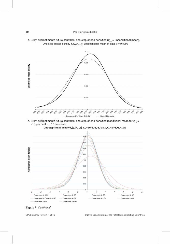
a. Brent oil front month future contracts: one-step-ahead densities (xt−1 = unconditional mean).

b. Brent oil front month future contracts: one-step-ahead densities (conditional mean for xt−1 = −10 per cent . . . 10 per cent).

Figure 9 Continued



d. Brent oil front month future contracts: conditional variance functions.

c. Brent oil front month future contracts: Gauss–Hermite quadratures.

Figure 9 Continued



more information than the SV-model, giving us conditional one-step-ahead densities.Based on the observation at day t it is therefore of interest to use the one-step-aheadstandard deviation for several applications. This filtered volatility and the Gauss–Hermite quadrature shown in plot (c) can be used for one-step-ahead price calculationsof any derivative. Figure 9d reports the conditional variance function. The functionreports the one-step-ahead dynamics of the conditional variance plotted against percent-age growth (δ). Here we can interpret the graph as representing the consequences of ashock to the system that comes as a surprise to the economic agents involved. Asymme-try (‘leverage effect’) can be evaluated from this function. From the shock (δ) contractplots, we find that the responses from negative (positive) shocks are much higher(lower) than from positive (negative). The SV model negative ρ− parameter with a modeof −0.578 and a standard error of 0.135 signals a significant negative mean and volatilitycorrelation. The asymmetry seems therefore important for the SV-specification’s meanand volatility paths.

Figure 9e reports multistep-ahead dynamics.The conditional volatility plots reveal thefuture dynamic response of system forecasts to contemporaneous shocks to the system.These generally non-linear profiles can differ markedly when the sign of δ changes.

e. Brent oil front month future contracts: multistep-ahead dynamics.

Figure 9 Future contracts: one-step-ahead unconditional (a) and conditional (b) mean; Gauss–Hermite quadrature (c); conditional variance function (d); and multistep-ahead dynamics (e).



However, the dynamics for the electricity market seems symmetric (+/−δ). Moreover,higher shocks are mean reverting while lower volatility shocks induce higher volatility tocome. Finally, profile bundles for the volatility are used to assess persistence. The profilebundles are over plots conditional to each observed datum. In fact, the profiles bundles arecode for the conditional profiles in a loop. If the thickness of the profiles bundle tends tocollapse to zero rapidly, the process reverts to its mean and if the thickness tends to retainits width, then the process is persistent (plots are not reported). The mean collapses rapidlyshowing mean reversion while the volatility retains its width showing persistence. Specifi-cally, the calculation of half-life (regression on margins) reveals approximately 19 dayswith associated standard error of 1.14 days. All these findings from the post-estimationanalysis add more insight to building scientifically valid models. Based on these findingsthe post estimation analysis seems to add insight to building scientifically valid models forEuropean energy markets.

Finally, for later applications, the most predominant applications for the SV model andre-projection methodologies are option pricing for implied volatility calculations andmarket risk premiums. From the long simulation (250 k) from the previous section wehave obtain SV-model asset mean and volatility estimates. Using this long simulationof { *, *}y xt t from our optimal SV structural model and performing a re-projection toget y f y x dyK* * | * *ˆ ( )∫ , where y* is unobserved (volatility) and x* observed (returns)variables, establishes the needed and highly valuable re-projected volatility. Assetprices Si,t are calculated every day from y* eventually producing Si,T at time Tusing risk neutral valuation (martingales). The fair price for a call is generallyc e E S X e x X f x dxrT Q

TrT

QX= −( )[ ] = −( ) ( )− − ∞

∫max , 0 and would be estimated by

c e N S XNrT

i Ti

N

= ( ) −( )−

=∑ max ,, 0

1

, where X is the strike price. A put option would be

estimated by p e N X SNrT

i Ti

N

= ( ) −( )−

=∑ max ,, 0

1

. Moreover, the fact that we now have

both the (un-)conditional and market implied volatilities from options available, marketrisk premiums can be calculated. For the Brent oil future contracts the risk premiums seemto vary between −35 per cent and −45 per cent and seem to rise towards maturity. The workfor pricing options, implied volatilities and risk premiums using re-projected volatilitywill soon be available for the ICE energy markets.17

7. Summary and conclusions

This paper has used the Bayesian M–H estimator and GSM for a SV representation for theEuropean financial energy market contracts. The methodology is based on the simple rule:compute the conditional distribution of unobserved variables given observed data. Theobservables are the asset prices and the un-observables are a parameter vector, and latent



variables. The inference problem is solved by the posterior distribution. Based on theClifford–Hammersley theorem (Hammersley and Clifford, 1970), p(θ,x|y) is completelycharacterised by p(θ|x,y) and p(x|θ,y).The distribution p(θ|x,y) is the posterior distributionof the parameters, conditional on the observed data and the latent variables. Similarly, thedistribution p(x|θ,y)is the smoothing distribution of the latent variables given the param-eters. The MCMC approach therefore extends model findings relative to non-linearoptimisers by breaking ‘curse of dimensionality’ by transforming a higher dimensionalproblem, sampling from p(θ1,θ2), into easier problems, sampling from p(θ1|θ2) andp(θ2|θ1) (using the Besag, 1974 formula).

The successful use of this version of the SV model for the European energymarkets suggests positive serial correlation in the mean and the volatility tends tocluster. Significant negative correlation between the mean and volatility induces nega-tive asymmetry and leverage effects. Although price processes are hardly predictable,the variance of the forecast error is time dependent and can be estimated by meansof observed past variations. The result suggests that volatility can be forecasted. More-over, observed volatility clustering induce an unconditional distribution of returns atodds with the hypothesis of normally distributed price changes. The SV models aretherefore an area in empirical financial data modelling that is fruitful as a practicaldescriptive and forecasting device for all participants/managers in the financial servicessector together with a special emphasis on risk management (forecasting/re-projectionsand VaR/Expected shortfall) and portfolio management (option contract pricesand Greek letters). In fact, the SV models are easy to simulate and the re-projectionmethodology can therefore be extended to option pricing and elaborate market riskmanagement.

Irrespective of markets and contracts, Monte Carlo Simulations should lead us to moreinsight of the nature of the price processes describable from SV models. Our findingssuggest that the ICE energy market is well-described using two-factor scientific SVmodels. The Bayesian MCMC methodology, the parallel central processing unit (CPU)execution and the M–H algorithm are computationally intensive for estimation, inferenceand assessment of model adequacy. Based on the simulated series the methodologyextends information to the market participants (density forecasts); the conditional meanand volatility (conditional moments), forecasting conditional volatility (filtering), condi-tional variance functions for asymmetry (smoothing) and multiple-ahead dynamics (meanreversion/persistence analysis).

Importantly, the price of a derivative of forwards/futures may not be possible to deter-mine, due to the inherent nature of latent SV. The reason is that there may not exist a self-financing portfolio strategy involving forwards/futures and risk-less bonds applying atracking portfolio approach with perfect replication of the derivatives pay-off (an incom-plete market).



Notes

1. The InterContinental Exchange (ICE): http://www.theice.com; The ICE provides trading andclearing of international power derivatives, European Union allowances (EUAs) and certifiedemission reductions (CERs).

2. The cointegration argument is analysed in several international studies. The mostcomprehensive studies are de Jong and Schneider (2009), Westgaard et al. (2010), Veka et al.(2012) and references therein.

3. The methodology is designed for estimation and inference for models where (i) thelikelihood is not available, (ii) some variables are latent (unobservable), (iii) the variables canbe simulated and (iv) there exists a well-specified and adequate statistical model for thesimulations. The methodologies [General Scientific Models (GSM) and Efficient Method ofMoments (EMM)] are general-purpose implementation of the Chernozhukov and Hongestimator (2003). That is, the applications for methodologies are not restricted to simulationestimators.

4. Using only market-traded products avoid the continuous-time no-arbitrage condition.5. The opening phase lasts approximately 5 minutes (the opening auction).6. The largest returns are found during the financial turmoil period in 2008/2009. The daily

price changes have decreased from 2009 until 2014.7. See for example Paolella and Taschini (2008) and Benz and Trück (2009) for applications in

energy markets. ARCH studies of energy markets are numerous and are often described asSV, but we do not follow that nomenclature. In the SV approach the predictive distribution ofreturns is specified indirectly, via the structure of the model, rather than directly as forARCH. However, the accompanying statistical model for the MCMC estimation in this paperis a non-parametric-ARCH model.

8. High frequency data based on the concept realised volatility are tied to continuous-timeprocesses and SV models.

9. For the Cholesky decomposition methodology see Bau III and Trefethen (1997).10. See www.econ.duke.edu/webfiles/arg for software and applications of the MCMC Bayesian

methodology. All models are coded in C++ and executable in both serial and parallel versions(OpenMPI).

11. The original statistical fit-model and the re-tuned assessment model with κ = 20 give roughlythe same parameter (η) results.

12. All the not reported tables, graphs and other materials (including software) are available fromthe authors upon request.

13. A quadratic fit is used and solved for the point where the quadratic equals the chi-square 1 df.critical value 3.841.

14. For applications of the EVT, it is important to check for log-linearity of the Power Law(Prob(υ > x) = Kx−α).

15. We use a transformation for lags of xt to avoid the optimisation algorithm using an extremevalue in xt−1 to fit an element of yt nearly exactly and thereby reducing the correspondingconditional variance to near zero and inflating the likelihood (endemic to all procedures



adjusting variance on the basis of observed explanatory variables). The trigonometric spline

transformation is: ˆ

arctan

x

x x x

x xi

i i tr tr i tr

i tr i=+ +( )[ ]( ) −{ } −∞ < < −

− < <1 2 4 4π π σ σ σ

σ σ ttr

i i tr tr tr ix x x1 2 4 4+ −( )[ ]( ) +{ } < < ∞

⎧⎨⎪

⎩⎪ π π σ σ σarctan

. The

transformation has negligible effect on values of xi between −σtr and +σtr but progressivelycompress values that exceed ±σtr so they can be bounded by ±2σtr.

16. A Gaussian quadrature over the interval (−∞, +∞) with weighting function W x e x( ) = − 2

(Abramowitz and Stegun, 1972, p. 890). The abscissas for quadrature order n aregiven by the roots xi of the Hermite polynomials Hn(x), which occur symmetricallyabout 0. An expectation with respect to the density can be approximated as:

E g y g abcissa j weight jj

npts

( )( ) = [ ]( )⋅ [ ]=

∑1

.

17. When up-to-date re-projected volatility is calculated and available the pricing caneasily be implemented in for example the Excel spreadsheet for any derivativefunction.

References

Abramowitz, M. and Stegun, I.A. (eds) 1972. Handbook of Mathematical Functions withFormulas, Graphs, and Mathematical Tables, 9th printing. NewYork, Dover,pp. 890.

Andersen, T.G., 1994. Stochastic autoregressive volatility: A framework for volatility modelling.Mathematical Finance 4, 75–102.

Andersen, T.G., Benzoni, L. and Lund, J., 2002. Towards an empirical foundation forcontinuous-time equity return models. Journal of Finance 57, 1239–1284.

Ané, T. and Geman, H., 2000. Order flow, transaction clock and normality of asset returns. Journalof Finance 55, 5, 2259–2284.

Bansal, R. and Yaron, A., 2004. Risks for long run: A potential resolution of asset pricing puzzles.Journal of Finance 59, 1481–1509.

Barberis, N., Huang, M. and Santos, T., 2001. Prospect theory and asset prices. Quarterly Journalof Economics 116, 1–54.

Bau, D., III and Trefethen, L.N., 1997. Numerical Linear Algebra. Philadelphia, PA, Society ofIndustrial and Applied Mathemathics.

Benth, F.E. and Koekebakker, S., 2008. Stochastic modeling of financial electricity contracts.Energy Economics 30, 3, 1116–1157.

Benth, F.E., Benth, J.S. and Koekebakker, S., 2008. Stochastic Modelling of Electricity andRelated Markets,. London, World Scientific Publishing Co. Pte. Ltd.

Benz, E. and Trück, S., 2009. Modeling the price dynamics of CO2 emission allowances. EnergyEconomics 31, 1, 4–15.

Besag, J., 1974. Spatial interaction and the statistical analysis of lattice systems (with discussion).Journal of Royal Statistical Society Series B 36, 192–326.



Bjerksund, P., Rasmussen, H. and Stensland, G., 2000. Valuation and risk management in theNordic electricity market, Working Paper, Institute of Finance and Management Science,Norwegian School of Economics and Business Administration.

Brigo, D. and Mercurio, F., 2001. Interest Rate Models—Theory and Practice. Berlin/Heidelberg,Springer-Verlag.

Brock, W.A., Dechert, W.D., Scheinkman, J.A. and LeBaron, B., 1996. A test for independencebased on the correlation dimension. Econometric Reviews 15, 197–235.

Campbell, J.Y. and Cochrane, J., 1999. By force of habit: A consumption-based explanation ofaggregate stock market behavior. Journal of Political Economy 107, 205–251.

Chernov, M., Gallant, A.R., Ghysel, E. and Tauchen, G., 2003. Alternative models for stock pricedynamics. Journal of Econometrics 56, 225–257.

Chernozhukov, V. and Hong, H., 2003. An MCMC approach to classical estimation. Journal ofEconometrics 115, 293–346.

Clark, P.K., 1973. A subordinated stochastic Process model with finite variance for speculativeprices. Econometrica: Journal of the Econometric Society 41, 135–156.

Clewlow, L. and Strickland, C., 2000. Energy Derivatives: Pricing and Risk Management.London, Lacima Publications.

de Jong, C. and Schneider, S., 2009. Cointegration between gas and power spot prices. The Journalof Energy Markets 2, 3, 1–20.

Durham, G., 2003. Likelihood-based specification analysis of continuous-time models of theshort-term interest rate. Journal of Financial Economics 70, 463–487.

Engle, R. and Kroner, K.F., 1995. Multivariate Simultaneous Generalized ARCH. EconometricTheory 11, 1, 122–150.

Gallant, A.R. and McCulloch, R.E., 2011. GSM: A program for determining general scientificmodels. Duke University. URL http://econ.duke.edu/webfiles/arg/gsm.

Gallant, A.R. and Tauchen, G., 1992. A nonparametric approach to nonlinear time series analysis.,estimation and simulation. In: Brillinger, D., Caines, P., Geweke, J., Parzan, E., Rosenblatt, M.and Taqqu, M.S. (eds) New Directions in Time Series Analysis, Part II. NewYork,Springer-Verlag, pp. 71–92.

Gallant, A.R. and Tauchen, G., 1998. Reprojecting partially observed systems with applicationto interest rate diffusions. Journal of the American Statistical Association 93, 441,10–24.

Gallant, A.R. and Tauchen, G., 2010a. Simulated score methods and indirect inference forcontinuous time models, Chapter 8. In: Aït-Sahalia, Y. and Hansen, L.P. (eds) Handbook ofFinancial Econometrics. Kidlington, Oxford, North Holland, pp. 199–240.

Gallant, A.R. and Tauchen, G., 2010b, EMM: A program for efficient methods of momentsestimation. Duke University. URL http://econ.duke.edu/webfiles/arg/emm.

Gallant, A.R., Hsieh, D.A. and Tauchen, G., 1991. On fitting a recalcitrant series: the pound/dollarexchange rate, 1974–83, Chapter 8. In: Barrett, W.A., Powell, J. and Tauchen, G.E. (eds)Nonparametric and Semiparametric Methods in Econometrics and Statistics, Proceedings ofthe Fifth International Symptosium in Economic Theory and Econometrics. Cambridge,Cambridge University Press, pp. 199–240.



Gallant, A.R., Hsieh, D.A. and Tauchen, G., 1997. Estimation of stochastic volatility models withdiagnostics. Journal of Econometrics 81, 159–192.

Hammersley, J. and Clifford, P., 1970. Markov fields on finite graphs and lattices. Unpublishedmanuscript.

Hansen, L.P., 1982. Large sample properties o generalized method of moments estimators.Econometrics 50, 1029–1054.

Hull, J. and White, A., 1987. The pricing of options on assets with stochastic volatilities. Journalof finance 42, 281–300.

Keppo, J., Audet, N., Heiskanen, P. and Vehvilinen, I., 2004. Modelling electricity forward curvedynamics in the Nordic market. In: Bunn, D.W. (ed.) Modelling Prices in CompetitiveElectricity Markets, Series in Financial Economics. Chichester, West Sussex, Wiley, pp.251–264.

Kiesel, R., Schindlmayer, G. and Börger, R., 2009. A two-factor model for the electricity forwardmarket. Quantitative Finance 9, 3, 279–287.

Kwiatowski, D., Phillips, P.C.B., Schmid, P. and Shin, T., 1992. Testing the null hypothesis ofstationary against the alternative of a unit root: How sure are we that economic series have aunit root. Journal of Econometrics 54, 159–178.

Ljung, G.M. and Box, G.E.P., 1978. On a measure of lack of fit in time series models. Biometrika66, 67–72.

Musiela, M. and Rutkowski, M., 1997. Martingale Methods in in Financial Modelling.Berlin/Heidelberg, Springer-Verlag.

Paolella, M. and Taschini, L., 2008. An econometric analysis of emission trading allowances.Journal of Banking and Finance 32, 10, 2022–2032.

Rosenberg, B., 1972. The behavior of random variables with nonstationary variance and thedistribution of security prices. Unpublished paper, Berkeley, Research Program in Finance,University of California.

Schwarz, G., 1978. Estimating the dimension of a model. Annals of Statistics 6, 461–464.Shephard, N., 2004. Stochastic Volatility: Selected Readings. NewYork, Oxford University Press.Tauchen, G. and Pitts, M., 1983. The price variability–volume relationship on speculative markets.

Econometrica: Journal of the Econometric Society 51, 485–505.Taylor, S., 1982. Financial returns modelled by the product of two stochastic processes—A study

of daily sugar prices 1961–79. In: Anderson, O.D. (ed.) Time Series Analysis: Theory andPractice, Vol. 1. Amsterdam, North-Holland, pp. 203–226.

Taylor, S., 2005. Asset Price Dynamics, Volatility, and Prediction. Princeton, New Jersey,Princeton University Press.

Veka, S., Lien, G., Westgaard, S. and Higgs, H., 2012. Time-varying dependency in Europeanenergy markets: An analysis of Nord Pool, European Energy Exchange and IntercontinentalExchange energy commodities. The Journal of Energy Markets 5, 2, 3–32.

Westgaard, S., Estenstad, M., Seim, M. and Frydenberg, S., 2010. Co-integration of ICE gas oiland crude oil futures. Energy Economics 33, 2, 311–320.



Opec 12048 rev2

Economy & Finance

Transcript of Opec 12048 rev2