OpAccess Derivinglamplikcationlfactorsl ... · Derivinglamplikcationlfactorsl...

Boudghene Stambouli et al. Earth, Planets and Space (2017) 69:99 DOI 10.1186/s40623-017-0686-3

FULL PAPER

Deriving amplification factors from simple site parameters using generalized regression neural networks: implications for relevant site proxiesAhmed Boudghene Stambouli1* , Djawad Zendagui1, Pierre‑Yves Bard2 and Boumédiène Derras1

Abstract

Most modern seismic codes account for site effects using an amplification factor (AF) that modifies the rock accelera‑tion response spectra in relation to a “site condition proxy,” i.e., a parameter related to the velocity profile at the site under consideration. Therefore, for practical purposes, it is interesting to identify the site parameters that best control the frequency‑dependent shape of the AF. The goal of the present study is to provide a quantitative assessment of the performance of various site condition proxies to predict the main AF features, including the often used short‑ and mid‑period amplification factors, Fa and Fv, proposed by Borcherdt (in Earthq Spectra 10:617–653, 1994). In this context, the linear, viscoelastic responses of a set of 858 actual soil columns from Japan, the USA, and Europe are com‑puted for a set of 14 real accelerograms with varying frequency contents. The correlation between the corresponding site‑specific average amplification factors and several site proxies (considered alone or as multiple combinations) is analyzed using the generalized regression neural network (GRNN). The performance of each site proxy combination is assessed through the variance reduction with respect to the initial amplification factor variability of the 858 profiles. Both the whole period range and specific short‑ and mid‑period ranges associated with the Borcherdt factors Fa and Fv are considered. The actual amplification factor of an arbitrary soil profile is found to be satisfactorily approximated with a limited number of site proxies (4–6). As the usual code practice implies a lower number of site proxies (gener‑ally one, sometimes two), a sensitivity analysis is conducted to identify the “best performing” site parameters. The best one is the overall velocity contrast between underlying bedrock and minimum velocity in the soil column. Because these are the most difficult and expensive parameters to measure, especially for thick deposits, other more conveni‑ent parameters are preferred, especially the couple (Vs30, f0) that leads to a variance reduction in at least 60%. From a code perspective, equations and plots are provided describing the dependence of the short‑ and mid‑period ampli‑fication factors Fa and Fv on these two parameters. The robustness of the results is analyzed by performing a similar analysis for two alternative sets of velocity profiles, for which the bedrock velocity is constrained to have the same value for all velocity profiles, which is not the case in the original set.

Keywords: 1D linear site response, Site proxies, Amplification factors, Neural network

© The Author(s) 2017. This article is distributed under the terms of the Creative Commons Attribution 4.0 International License (http://creativecommons.org/licenses/by/4.0/), which permits unrestricted use, distribution, and reproduction in any medium, provided you give appropriate credit to the original author(s) and the source, provide a link to the Creative Commons license, and indicate if changes were made.

Open Access

*Correspondence: [email protected] 1 Risk Assessment and Management Laboratory (RISAM), Faculté de Technologie, Université Abou Bekr Belkaïd, BP 230‑13048, Tlemcen, AlgeriaFull list of author information is available at the end of the article

http://orcid.org/0000-0001-6948-5235

http://creativecommons.org/licenses/by/4.0/

http://crossmark.crossref.org/dialog/?doi=10.1186/s40623-017-0686-3&domain=pdf

of 26Boudghene Stambouli et al. Earth, Planets and Space (2017) 69:99

IntroductionIt is recognized that site effects have a great impact on seismic ground motion and could thus cause increased damage to structures. For instance, during the Michoa-can Earthquake of Mexico (e.g., Anderson et al. 1986; Hall and Beck 1986; Esteva 1988; Singh et al. 1988a, b; Bard et al. 1988; Romo et al. 1988; Seed et al. 1988; Sanchez-Sesma et al. 1988; Kawase and Aki 1989; Singh and Ordaz 1993; Chávez-García and Bard 1994; Cruz-Atienza et al. 2016) amplification induced from site effects has been recognized as the major cause of struc-tural collapse.

In this study, seismic amplification is measured with an amplification factor (AF), defined as the ratio of response spectra between soil surface and outcropping reference rock. Among many other parameters characterizing the intensity of ground motion, response spectra are the most used in engineering practice. Most building codes use response spectra to define design earthquake loads on engineered structures. Most hazard assessment stud-ies use acceleration response spectra to define the seis-mic motion through ground motion prediction equations (GMPEs) that correlate the spectral ordinates to magni-tude, distance, and site parameters. In most GMPEs, the site conditions are described with a single-site proxy; currently, the most common is the “Vs30” parameter, cor-responding to the harmonic average of S-wave velocity over the top 30 m, first introduced by Borcherdt (1994), which has, since then, been widely used (see, for instance, Martin and Dobry 1994; Dickenson and Seed 1996; Dobry et al. 2000; Rodriguez-Marek et al. 2001; Pitila-kis et al. 2001). Almost all recent GMPEs, for instance, the NGA (Abrahamson et al. 2008), NGAWest2 (Gregor et al. 2014; Ancheta et al. 2014), and GMPEs derived from the RESORCE database (Douglas et al. 2014) still rely on Vs30 to describe site conditions. It is sometimes complemented or replaced by other site parameters, such as the fundamental frequency f0 (Castellaro et al. 2008; Luzi et al. 2011; Cadet et al. 2012; Pitilakis et al. 2012, 2013) or depth to a hard bedrock level defined with a threshold velocity (from 1 to 2.5 km/s; see Ancheta et al. 2014). The terms associated to such site proxies provide a mechanism for quantifying the frequency-dependent “amplification factor” with respect to “standard rock” (usually characterized by Vs30 = 760 to 800 m/s). The same proxies are also used in regulatory codes to tune the characteristics of design spectra, i.e., peak ground accel-eration (PGA), plateau bandwidth and level, and long-period decay, to the site conditions. For instance, this is the case for the major building codes used at the interna-tional level, i.e., International Building Code (IBC 2012), Uniform Building Code (UBC 1997), and Eurocode 8 (EC8 2004).

However, these site proxies are too simple and too few to capture the entire physics of site amplification, and distinct sites with similar site proxy values (e.g., Vs30) could have different amplification characteristics. This has at least two consequences. First, it significantly impacts the aleatory variability of GMPEs by increasing the within-event term, which in turn increases the hazard estimates, especially at long return periods. Second, cor-responding site terms may exhibit significant variations from one GMPE to another, depending on the strong motion data used for their derivation. For instance, the relationship between Vs30 and deeper velocity structure is not identical in the Los Angeles basin, Japanese coastal plains, or intra-mountain basins in the Alps or the Apen-nines; therefore, the associated long- or short-period effects may differ. The issue addressed in this paper is to identify the best site parameters that optimally explain, and therefore predict, the actual site-specific amplifica-tion factor. The aim is to derive “stand-alone” site terms, which could be applied as a post-processing step to any rock GMPEs.

With that aim in mind, the focus here is on the 1D response of horizontally stratified soil columns, and on investigating the relationships between corresponding amplification factors on response spectra, and limited number of “site proxies” describing the overall character-istics of the soil profile. A series of 858 real soil profiles are considered, and their linear viscoelastic responses to vertically incident S waves are computed for 14 dis-tinct, real input waveforms spanning a wide range of frequency contents. For each site, the geometric aver-age amplification factor is derived from these 14 differ-ent loadings, and an artificial neural network approach is used to investigate the correlation between this aver-age amplification factor and various sets of soil charac-teristics. Sensitivity studies are performed to identify the relative performance of several site proxies, with the goal of proposing optimal combination sets offering a good compromise between physical relevancy and prac-tical affordability. The robustness of the results is tested by conducting the same analysis on two additional sets of soil profiles, termed normalized soil profiles (NP) and truncated soil profiles (TP), modified to correspond to a uniform bedrock velocity of 800 m/s.

Derivation of amplification factors (AF)IntroductionThis section describes the overall procedure to obtain a set of amplification factors for several hundreds of real-istic soil profiles. For a particular soil profile and input motion, the amplification factor is computed as the ratio of response spectra at the soil surface to response spectra at the outcropping reference rock.


where SA(T )s and SA(T )b are, respectively, the 5% response spectra at the site surface and outcropping ref-erence bedrock, while T is the structural period. They are obtained as follows:

1. Choose a soil profile S and use the 1D viscoelastic analysis to derive the corresponding Fourier transfer function T

(

f)

2. Select a reference rock motion b(t) and compute its Fourier transform B(f ) together with its 5% accelera-tion response spectrum SA(T )b

3. Compute the Fourier transform of motion at the soil surface As

(

f)

by multiplying B(f ) by T(

f)

4. Perform an inverse Fourier transform on As

(

f)

to obtain the surface motion in time domain as(t).

5. Derive the 5% acceleration response spectrum SA(T )s from as(t).

Once SA(T )s and SA(T )b are derived, the amplification fac-tor for site s and input b can be readily obtained from Eq. (1).

(1)AF(T ) =SA(T )s

SA(T )b

The next sections provide additional information for selected input accelerograms, followed by a short indi-cation on the way transfer functions, and thus, amplifi-cation factors are computed using classical concepts of wave propagation in horizontally stratified media. The considered site profiles are finally briefly described, from original soil profile information to selecting a small num-ber of site proxies, and providing their statistical distri-bution to assess the relevancy and validity domain of the study.

Seismic input SA(T)bFourteen input waveforms (S1–S14), recorded on out-cropping rock, are selected from the RESORCE data-base (Akkar et al. 2014). Their characteristics are listed in Table 1. The amplification factor defined in Eq. (1) depends on the frequency content of the seismic motion (see, for instance, Biro and Renault 2012; Renault et al. 2014; Bora et al. 2015, 2016). Therefore, it was decided to select real accelerograms, corresponding to near-source rock record-ings, with a wide range of spectral contents, and derive the geometrical mean of the amplification factors obtained for each accelerogram. As illustrated in Fig. 1, the spectral

Table 1 Main characteristics of the 14 reference acceleration time histories

Identification RESORCE Waveform Id

PGA (m/s2) Earthquake Station Mw Distance Site conditions

Peak frequency (highest PSA)

S1 16,149 1.269 Manjil (Iran) 20/06/1990

Zanjan 7.7 56 A f < 2 Hz

S2 16,351 1.288 Olfus (Iceland) 29/05/2008

Ljosafoss‑Hydroelec‑tric Power Station

6.1 11 A f < 2 Hz

S3 16,352 3.190 Olfus (Iceland) 29/05/2008

Selfoss City Hall 6.1 3 A f < 2 Hz

S4 15,537 2.074 South Iceland 17/06/2000

Thjorsarbru 5.0 10 A 2 Hz < f<4 Hz

S5 6756 3.106 South Iceland 17/06/2000

Flagbjarnarholt 6.6 15 A 2 Hz < f<4 Hz

S6 6765 3.140 South Iceland 17/06/2000

Thjorsarbrun 6.6 4 A 2 Hz < f<4 Hz

S7 583 1.003 Lazio‑Abruzzo 11/05/1984

Villetta Barrea 5.3 2 A 4 Hz < f<8 Hz

S8 16,974 1.474 L’Aquila 07/04/2009 (aftershock)

Pescomaggiore 5.3 10 A 4 Hz < f<8 Hz

S9 15,905 3.006 Firouzabad (Iran) 20/06/1994

Zarrat 5.8 11 A 4 Hz < f<8 Hz

S10 188 1.496 Basso Tireno 15/04/19878

Naso 5.5 16 A 4 Hz < f<8 Hz

S11 17,116 1.023 L’Aquila aftershock 09/04/2009

Montereale 4.9 10 A 8 Hz < f<16 Hz

S12 6802 4.260 South Iceland after‑shock 21/06/2000

Thjorsartun 6.4 3 A 8 Hz < f<16 Hz

S13 16,996 1.393 L’Aquila aftershock 07/04/2009

L’Aquila Via Aterna—Il Moror

4.2 2 A 8 Hz < f<16 Hz

S14 6789 0.803 South Iceland after‑shock 21/06/2000

Hveragerdi‑Church 6.4 23 A 8 Hz < f<16 Hz


shapes corresponding to each selected accelerogram, i.e., the response spectra normalized by the corresponding PGA, exhibit peak periods ranging from 0.07 s to slightly beyond 1 s, with four motions with peak periods in the range [0.0625–0.125 s], four in the range [0.125–0.25 s], three in the range [0.25–0.5 s], and three >0.5 s. The cor-responding PGA values are also listed in Table 1 (rang-ing from 0.8 to 4.2 m/s2), but actual PGA values have no importance in the present computations because only the linear response is considered. The main goal is to ensure a representative average amplification factor that is unbiased by spectral contents too rich in either short or long periods.

Theoretical derivation of the transfer function T(

f)

For a particular soil profile, the AF is computed once the transfer function T

(

f)

is known. In this study, 1D vis-coelastic soil behavior is considered. The soil is ideally composed of n horizontally layered soils deposit resting on a substratum that is termed bedrock (see Fig. 2). Each layer i is fully known by its thickness hi, shear modulus Gi or shear wave velocity Vi, damping ratio ζi, and mass density ρi. The underlying half-space has a shear wave velocity Vn+1 that is termed Vbedrock. The vertical z-axis is oriented downwards, and its origin is taken at the free surface. The top of each layer i is located at the depth zi−1, and its bottom at depth zi = zi−1 + hi. The response of the soil column to harmonic, vertically incident plane shear waves is governed by the equation (Kramer 1996):

(2)(1+ 2i ζi)∂2ui

∂z2= −

ω2

V 2i

ui

where ui is the horizontal displacement in the ith layer, ω is the angular frequency, and ζi is the damping ratio.

In each layer, the wave field can be described as the summation of an up-going and a down-going plane wave with unknown amplitudes Ai and Bi. Solving the stress and displacement continuity equations at each interface establishes the relationships between these amplitudes for two adjacent layers. These relationships can thus be propagated from the bottom (unit up-going amplitude) to top layer. Using the free surface condition, the wave amplitudes in the top layer can be derived, and the trans-fer function with respect to the motion at outcropping bedrock.

Since the pioneering work of Thomson (1950) and Haskell (1953), many codes such as SHAKE (Schnabel et al. 1973), DEEPSOIL (Hashash et al. 2012), or EERA (Bardet et al. 2000) have been developed that provide the transfer function in the linear domain. However, we developed our own MATLAB® code and verified its accuracy against DEEPSOIL and EERA.

In addition, the damping is estimated in relation to the quality factor QSi using the well-known equation:

(3)

ui(z,ω) =[

Aieiω(z−zi−1)/Vi + Bie

−iω(z−zi−1)/Vi

]

eiωt

(4)T(

f)

= u1(z = 0,ω)/2 = A1

10-1

100

1010

0.5

1

1.5

2

2.5

3

3.5

4

4.5

5

Period (s)

Nor

mal

ized

Spe

ctra

l Acc

eler

atio

n

S1S2S3S4S5S6S7SmS8S9S10S11S12S13S14

Fig. 1 Spectral content for the 14 input waveforms considered for the computation of amplification factors. Each thin curve represents the normalized acceleration response spectrum Sa,j(T )bedrock/pgaj of the jth acceleration waveform (j = 1–14), the thick solid line represents their geometrical mean Fig. 2 Schematic representation of the 1D site response analysis

method for a site consisting of n horizontal layers soils overlying bedrock. The parameters for each layer i are its thickness hi, shear modulus Gi, shear wave velocity Vi, damping ratio ζi, unit mass ρi, and thickness hi = zi − zi‑1


The S-wave quality factor Qi is estimated here as related to the S-wave velocity through a scaling factor SCQ, as described in Aki and Richards (1980) and Fukushima et al. (1995):

where SCQ is taken equal to 10 in the absence of meas-urements for all the profiles considered in this study.

Soil profiles, database, and site parametersOverview of soil profiles

a. Set 1: Real Profiles (RP)We consider three sets of soil profiles. The first one,

termed RP, is composed of nP = 858 soil profiles. It was originally compiled by C. Cornou (Salameh 2016; Sala-meh et al. 2017) and consists of about 600 Japanese KiK-net sites, more than 200 sites from the USA, made available by D. Boore (http://quake.usgs.gov/~boore), and 22 European sites measured during the NERIES pro-ject (Di Giulio et al. 2012). The main characteristics of this set of site profiles are presented in Salameh (2016), Almakari et al. (2016) and Salameh et al. (2017): They are primarily usual (i.e., normally soft, with S-wave velocities generally >200 m/s) and stiff soils, with shallow to inter-mediate thicknesses, <200 m in most cases, with only few sites—about 50—with fundamental frequency below 1 Hz. They generally have “normally hard” to very hard underlying bedrock; the “bedrock” velocity, i.e., the veloc-ity of the underlying half-space, varies from <500 m/s to >3 km/s.

Such variability in “bedrock” velocity is due to the velocity profile having been measured over a limited depth, not always reaching the underlying hard rock. Because part of the amplification is controlled by the velocity contrast, this variability may significantly bias the site response and assessment of the respective influ-ence of the various site proxies considered here. It is usually considered within the earthquake engineering community that amplification should be measured with respect to a “standard rock” reference site with a velocity around 800 m/s. Consequently, the real soil profiles have been modified to have a normalized bedrock velocity of 800 m/s.

b. Set 2: Normalized profiles (NP):

The second data set is termed NP and is derived from the RP set using a homothetic transformation; all veloci-ties are scaled by a factor of 800/Vbedrock so that the

(5)ζi =

1

2Qi

(6)QSi = Vi/SCQ

bedrock velocity is equal to 800 m/s for each profile in this “normalized profile” set, while the thickness of each layer is also scaled with the same factor to maintain an unchanged transfer function.

More specifically, for a site j with a bedrock velocity Vbedrock,j, the scaling is applied to the velocities and thick-nesses of all layers i (i = 1, Nj) as follows:

For real sites with very hard bedrock, e.g., Vbedrock = 2500 m/s, the scaled velocities may become unrealistically small at shallow depths; for instance, if V1 = 120 m/s, then, according to (7), V ′

1 = 40 m/s. Therefore, only normalized soil profiles with minimum scaled velocities exceeding 80 m/s are retained in this NP set, which reduces their number from 858 to 570.

c. Set 3: Truncated profile (TP)

The third set of soil profiles, termed TP, is derived sim-ply by performing a “truncation” of each real soil pro-file; velocities are kept unchanged from surface until the depth Z800, where the velocity first exceeds 800 m/s, and beyond this depth the velocity is set to 800 m/s. Whenever the bedrock velocity of the real soil profile is smaller than 800 m/s, the bedrock velocity is increased to 800 m/s. Therefore, this third TP set also consists of 858 soil profiles.

Site parametersEach soil profile in each of the three sets can be partially described with a few site parameters, often called site proxies. In the present study, we investigate six of them, which have already been proposed by various authors in view of site classification (see, for instance, Castellaro et al. 2008; Cadet et al. 2012; Pitilakis et al. 2012, 2013), and provide information on the stiffness and/or thick-ness of soil columns. These parameters are the depth to bedrock (Depth); average shear velocity (Vsm) over that depth, where subscript sm stands for mean value of the shear wave velocity; average shear wave velocity over the upper 30 m (Vs30); shear wave velocity of bedrock (Vbed-

rock); velocity contrast, i.e., ratio between shear wave velocities in bedrock and at the surface (Cv); and soil pro-file fundamental frequency ( f0). The exact definition of each of these six parameters is detailed below:

(7)V ′i,j = Vi,j · 800/Vbedrock,j

(8)h′i,j = hi,j · 800/Vbedrock,j

(9)Depth =n

∑

i=1

hi

http://quake.usgs.gov/%7eboore


Here, “bedrock” is the last known unit, which we con-sider as an underlying infinite half-space, while n is the number of layers above bedrock (see Fig. 2).

where Vi =√Gi/ρi is the shear wave velocity in layer (i).

where l30 is the number of distinct layers found in the top 30 m.

f0 = fundamental soil frequency corresponding to the first peak (not necessarily the highest in amplitude) in the transfer function. In this study, for the sake of simplicity, f0 is determined using the Simplified Version of the Ray-leigh Procedure (method # 7 in Dobry et al. 1976). Briefly, this approach is based on an approximation of the modal shape at the fundamental frequency, leading to the fol-lowing Eqs. (13) and (14).

where (zi+1 + zi)/2 is the depth of midpoint of layer (i) and Xi values correspond to the estimated fundamental mode shape at the top of each layer (i), derived according to Dobry et al. (1976):

Distribution of site parametersThe cumulative distributions of the log values of these six parameters are summarized in Fig. 3 for profile sets of RP, NP, and TP (more details can be found in Additional Files 1, 2, and 3, for each profile set, respectively). There is no distribution of Vbedrock for NP and TP sets, because it has a fixed value of 800 m/s. Most parameters follow a quasi-lognormal distribution, except for Vbedrock, which is significantly skewed with a mode at 3.2 km/s (Fig. 3 and Additional file 1), and is characterized by large variability.

Moreover, as these parameters are not fully independ-ent, the coefficient of determination (R2) between each pair of parameters has been computed and is listed in Table 2 for the three RP, NP, and TP sets. There is an overall tendency for some correlation between velocity

(10)Vsm =n

∑

i=1

hi

/

n∑

i=1

hi

Vi

(11)Vs30 = 30

/

l30∑

i=1

hi

Vi

(12)Cv =VBedrock

V1

(13)

f0 =

√

(

4

(

∑ni=1

(zi+zi+1)2

V 2i

hi

)/

(∑n

i=1(Xi + Xi+1)

2hi)

)

2π

(14)Xn = 0. ; Xi−1 = Xi +zi + zi−1

V 2i

hi

parameters, especially Vsm and Vs30, but also the bedrock velocity VBedrock and Vsm, Vs30 and Cv, while much weaker correlations (R2 between 0.1 and 0.02) are observed for the parameter pairs

(

Cv , f0)

, (Depth,VS30), (Depth,Cv) and (Depth,VBedrock). These correlation indicators are useful for selecting independent site parameters for the models relating site amplification to site characteristics.

Computed amplification factors: main statistical characteristicsGeneral backgroundThis section presents on overview of the computed sets of frequency-dependent AF, and their short- and mid-period average values (i.e., the Borcherdt factors Fa and Fv). This is essential as they constitute the learning set to identify the key parameters controlling the characteris-tics of site response.

AF values (Eq. 1) are calculated for the soil profiles RP, NP, and TP subjected to 14 seismic excitations. They may be written AF(Pk , θ , Sl ,Ti), where:

• Pk , k = 1, . . . nP is introduced to identify the soil profile. Note that for RP and TP nP = 858 and for NP nP = 570 because we have imposed the minimal value of V ′

1 as 80 m/s • θ = 0 for RP, θ = 1 for NP, and θ = 2 for TP. • Sl , l = 1, 14 is the lth excitation. Note that, as indi-

cated below, the geometrical average of the 14 ampli-fication factors has been computed for each site.

• Ti, (i = 1, . . . 271) is the ith structural period. AF values are systematically computed for 271 values, equally spaced between 0.01 and 10 s on a logarith-mic period axis, i.e., also equally spaced between 0.1 and 100 Hz on a logarithmic frequency axis.

For instance, AF(P20, 2, S8,T55) stands for the AF obtained at the 50th period T55 for the truncated soil pro-file P20 subjected to seismic excitation S8. After the AF is calculated for a particular profile k, and 14 seismic excita-tions, the site average amplification factor is computed as the geometrical average of the 14 individual amplification factors:

Hereafter, the abridged notation AF will stand for the average value AFm(Pk , θ ,Ti).

Simultaneously, for each profile Pk, AF variability derived from the 14 different time histories is quantified using the corresponding standard deviation:

(15)

log [AFm(Pk , θ ,Ti)] =(

1

14

) 14∑

l=1

log [AF(Pk , θ , Sl ,Ti)]


1 10 100 10000

0.1

0.2

0.3

0.4

0.5

0.6

0.7

0.8

0.9

1

Depth(m)

RPNPTP

0.1 1 10 20 30 50 1000

0.1

0.2

0.3

0.4

0.5

0.6

0.7

0.8

0.9

1

f0(hz)

RPNPTP

1 10 20 1000

0.1

0.2

0.3

0.4

0.5

0.6

0.7

0.8

0.9

1

Cv

RPNPTP

100 200 400 600 1000 15000

0.1

0.2

0.3

0.4

0.5

0.6

0.7

0.8

0.9

1

Vsm

(m/s)

RPNPTP

10 100 200 400 600 1000 15000

0.1

0.2

0.3

0.4

0.5

0.6

0.7

0.8

0.9

1

Vs30

(m/s)

RPNPTP

100 200 400 600 1000 1500 2000 30000

0.1

0.2

0.3

0.4

0.5

0.6

0.7

0.8

0.9

1

VBedrock

(m/s)

RP

Fig. 3 Cumulative distribution functions of the six selected site parameters for the soil profile sets of RP, NP, and TP; there are only five parameters for the two latter sets


(16)σAF(Pk , θ ,Ti) =

√

∑14l=1 [log (AF(Pk , θ , Sl ,Ti))− log (AFm(Pk , θ ,Ti))]

2

14

Table 2 Correlation between the various site parameters for the three profile sets (RP, NP, and TP, from top to bottom)

The values in the cells correspond to the coefficient of determination R2 between the corresponding site parameters)

RP

RP Depth f0 Cv Vsm Vs30 Vbedrock

Depth 1 0.3441 0.0903 0.2434 0.0388 0.0962

f0 1 0.0196 0.1858 0.4050 0.3102

Cv 1 0.1596 0.0559 0.5345

Vsm 1 0.8515 0.6784

Vs30 1 0.5531

Vbedrock 1

NP

NP Depth f0 Cv Vsm Vs30

Depth 1 0.4933 0.2137 0.4227 0.0299

f0 1 0.0300 0.3680 0.1218

Cv 1 0.5297 0.5333

Vsm 1 0.8423

Vs30 1

TP

TP Depth f0 Cv Vsm Vs30

Depth 1 0.4176 0.1973 0.2430 0.0664

f0 1 0.3864 0.0629 0.2529

Cv 1 0.3852 0.5436

Vsm 1 0.8811

Vs30 1

0.1 1 100

0.05

0.1

0.15

0.2

0.25

0.3

0.35

Period(s)

Ampl

ificat

ion

fact

or v

aria

bility

Fig. 4 Variability of amplification factors with spectral contents of the reference rock motion. Each thin line corresponds to the variability of one of the 858 1D profiles considered here. The thick red line cor‑responds to the average signal‑to‑signal variability for all profiles

The σAF values are displayed in Fig. 4 for all 858 sites; they exhibit a significant frequency dependence, decreasing from ~0.1 at short period to ~0.03 at intermediate and long periods. These values are quite significant, especially at short periods; it would thus be meaningless to seek extremely precise models with residuals between obser-vations and predictions much below these values.

A few additional parameters are introduced to measure the variability of the results.

• Average AF for all profiles, noted AF0(θ ,Ti) and defined as the geometrical average of the np average AF (AF(Pk , θ ,Ti)) noted for simplicity as AF0:

(17)log (AF0(θ ,Ti)) =1

np

np∑

k=1

[log (AFm(Pk , θ ,Ti))]


• Initial variability, defined as the initial standard devi-ation of the site average amplification factor over all profiles

• Maximum initial variability, defined as the peak value of the initial variability σ0 over the whole period range:

• Overall initial variability, defined as the average over all periods of initial variability

where nT is the number of structural periods (or fre-quencies) used, i.e., 271.

Means and variability of AFFor each profile set, we compute the nP × 14 AF: AF(Pk , θ , Sl ,Ti), the nP average amplification factors AFm: AFm(Pk , θ ,Ti) together with their corresponding vari-ability σAF(Pk , θ ,Ti). We then derive the mean amplifi-cation factor AF0(θ ,Ti) and associated initial variability σ0(θ ,Ti) . The results are displayed in Fig. 5a, b, and c for each of the three RP, NP, and TP profile sets, respectively. The following observations are made.

• The peak period, i.e., the period with peak amplifica-tion, covers a broad range, from 0.08 s to about 3–4 s for the RP set, and from 0.1 s to about 1–2 s for the NP and TP sets.

• The corresponding peak amplification ranges from less than 1.5 up to 15. The highest peak (almost 15) is observed for RP, whereas for NP and TP the peak is less than 4.

• Some amplification factors exhibit a short-period de-amplification; a careful look at the correspond-ing profiles indicates it corresponds to profiles with low-velocity zones at some depth that act as a (weak) seismic isolator.

• The overall average amplification factor is close to 1 at long period (because long wavelengths do not “feel” the site structure over the first hundred meters), and it exhibits a very smooth and broad maximum with a value around 2 between 0.1 and 0.2 s. It is slightly below 2 at very short periods. It is significantly smaller than the peak values for individual profiles, which emphasizes the need to identify some relevant site parameters that may explain this site-to-site variability

(18)

σ0(θ ,Ti) =

√

√

√

√

1

np

np∑

k=1

[

log(

AFm(Pk , θ ,Ti))

− log(

AF0(θ ,Ti))]2

(19)σOmax(θ) = MaxTi [σ0(θ ,Ti)]

(20)σ0m(θ) =1

nT

nT∑

i=1

σ0(θ ,Ti)

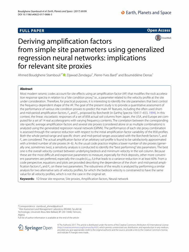
• The corresponding “initial variability” σ(θ ,Ti) is listed in Table 3 for RP, NP, and TP. It is maximum at intermediate periods (0.1–0.4 s, up to 45%) and mini-mum at long periods (around 10%).

Means and variability of AF in the normalized frequency domain As written in Eq. (15), AF can be described as a func-tion of period Ti, i.e., AF(Pk , θ ,Ti), or alternatively fre-quency, fi = 1/Ti. As indicated in Cadet et al. (2012), it may be helpful to normalize the frequency axis using the fundamental frequency of each site and compare all

0.1 1 10

1

2

3456

10

Period (s)

Am

plifi

catio

n fa

ctor

fa

fv

0.1 1 10

1

2

3

Period (s)

Am

plifi

catio

n fa

ctor

fa fv

0.1 1 10

1

2

3

4

5

Period (s)

Am

plifi

catio

n fa

ctor fa

fv

a

b

c

Fig. 5 Average amplification factors as a function of real period for each set of soil profiles. a RP (top), b NP (middle), and c TP (bottom). Thin blue lines correspond to every site profile, the thick red line is the geometrical average over the whole profile set, and thick light blue lines are the average ± one standard deviation


amplification factors as a function of the dimensionless normalized frequency ν = f /f0. Thus, AF can be rewrit-ten as AF(Pk , θ , νi), where νi = fi/f0. The corresponding plots of all amplification factors, together with the aver-age and average ± one standard deviation, are displayed in Fig. 6a, b, and c for RP, NP, and TP sets, respectively.

As shown, the starting and ending abscissas of the AF(Pk , θ , νi) curves vary between profiles because of the variability in f0 values. For instance, for two profiles 1 and 2 with f0 values, respectively, 2 and 10 Hz, and an investigated “absolute frequency” range [fmin = 0.1 Hz, fmax = 100 Hz], the normalized frequency ranges [νmin, νmax] are, respectively, [0.05, 50] and [0.01, 10]. The num-ber of available amplification factors thus varies with the normalized frequency ν, as displayed in Fig. 7 for the three sets of profiles. All curves exhibit a clear plateau centered on ν = 1, which systematically starts at ν = 0.1, but ends at varying values depending on the profile set, around ν = 10 for RP and NP, and around ν = 3 for TP. Within this range of normalized frequency values, about 90% of the considered profiles provide amplification fac-tor values. The corresponding average and variability, computed as indicated in Eqs. (15) to (20), have thus been calculated only for normalized frequencies ranging from 0.03 to 30, which corresponds to the availability of at least half the total number of profiles for each set (Fig. 7).

As shown in Fig. 6, the main consequences of this fre-quency normalization are to decrease the low-frequency scatter and slightly increase the mean AF values and associated scatter for ν = 1, while the “high-frequency” mean values and standard deviations are comparable

to the short-period values shown in Fig. 5 and listed in Table 4. More explicitly, the widespread scatter of “real frequency” amplification factors, due to the combined variability of fundamental frequencies and amplifica-tion values, is redistributed in the normalized frequency domain. This transfers the variability primarily around and beyond the fundamental frequency.

Focus on short and intermediate period (“Borcherdt factors” Fa and Fv)For a building code perspective, special attention is given to the short- and intermediate-period factors introduced

Table 3 Initial variability values for the amplification fac-tors in the real frequency domain for the RP, NP, and TP profile sets

RP–RF NP–RF TP–RF

Total initial variability σ0m 0.1178 0.0846 0.0896

Maximum initial variability σ0max 0.1717 0.1232 0.1317

σ (T = 0.01 s) 0.1227 0.0811 0.0866

σ (T = 0.02 s) 0.1226 0.0809 0.0861

σ (T = 0.04 s) 0.1206 0.0756 0.0759

σ (T = 0.07 s) 0.1314 0.0883 0.0861

σ (T = 0.1 s) 0.1494 0.1062 0.106

σ (T = 0.2 s) 0.1623 0.1169 0.1242

σ (T = 0.4 s) 0.1446 0.1089 0.1188

σ (T = 0.7 s) 0.1200 0.098 0.1093

σ (T = 1.0 s) 0.1040 0.0873 0.0982

σ (T = 2.0 s) 0.0626 0.0503 0.0552

σ (T = 4.0 s) 0.0477 0.033 0.036

σ (T = 7.0 s) 0.0388 0.027 0.0296

σ (T = 10.0 s) 0.0412 0.0297 0.0329

0.03 0.1 1 10 30

1

10

Normalized frequency (f/f0)

Am

plifi

catio

n fa

ctor

0.1 1 10 30

1

2

3


Am

plifi

catio

n fa

ctor

0.03 0,1 1 10 30

1

2

3

4

5


Am

plifi

catio

n fa

ctor

a

b

c

Fig. 6 Average amplification factors as a function of normalized fre‑quency for each set of soil profiles. a RP (top), b NP (middle), and c TP (bottom). Thin blue lines correspond to every site profile, the thick red line is the geometrical average over the whole profile set, and thick light blue lines are average ± one standard deviation


by Borcherdt (1994, 2002) to specify the short-period level (acceleration plateau) and intermediate-period level (velocity response). In the absence of any consensual, widely accepted definition, we defined them as follows:

• Fa is taken as the geometrical mean of AF for peri-ods in the range [0.1 s, 0.2 s]

• Fv is taken as the geometrical mean of AF for periods in the range [0.75 s, 1.5 s]

The corresponding period ranges are displayed in Fig. 5. Considering that the amplification factors were derived for equally spaced values on a logarithmic period axis, these two average values thus correspond to exactly the same number of points.

Resulting sets of AF and Borcherdt factorsThe methodology detailed in this section leads to three sets of amplification factors AF for RP, NP, and TP, which can be described as a function of real or normalized frequency. The three real frequency sets have also been summarized with the two Borcherdt factors, because these scalar values corresponding to the short and inter-mediate periods are widely used to translate the impact of site effects in building codes. The main issue now is to understand the influence of site parameters on shaping the values of both the AF and Borcherdt factors. To reach this goal, we use the generalized regression neural net-work (GRNN) approach, described in the next section.

Description of the neural network approachScope and principles of artificial neural networksIn general, the scope of the artificial neural network approach is to establish relationships, or classifications, between a set of output parameters and set of input parameters, which are too complex to be “guessed” using simple functional forms. It is based on a “learning phase,” where a large number of “known points,” with known input and output values, are used to train the neural net-work system in an “optimal” way, so that it can be later used to predict (unknown) output values for a new set of input values, that should fall in the domain of the hyper-space that is properly sampled by the learning data set. The flexibility of neural networks has fostered their use in many different disciplines for regression and classifi-cation purposes, where they have proven very powerful. For instance, in engineering seismology, they have been applied to site amplification issues (Giacinto et al. 1997; Paolucci et al. 2000), establishing GMPEs (see Derras et al. 2012 for a review of previous applications, and Der-ras et al. 2014, 2016 for recent developments), and gener-ating spectrum compatible time histories (Ghaboussi and Lin 1998; Lin and Ghaboussi 2001).

The objective of an ANN is to mimicking human brain behavior with interconnecting artificial neurons between input and output layers that contain input and output data, with very often hidden layers in between. Each neu-ron is a kind of microprocessor that connects two layers l and l + 1 through accepting a set of inputs from layer l, performing a weighted sum of all these inputs, and pro-cessing this weighted sum through an “activation func-tion,” which may be linear or nonlinear, and essentially makes this neuron “fire” when the input weighted sum is large enough.

The main degrees of freedom of an ANN, in addition to its architecture (number of hidden layers, and number of neurons in each of them), are the weights for each neuron (together with another parameter named the “bias,” see Derras et al. 2012) and shape of the activation function.

10-2

10-1

100

101

102

0

100

200

300

400

500

600

700

800

900


Num

bers

of p

rofil

es

RPNPTP

Fig. 7 Variation in the number of available profiles as a function of the normalized frequency ν = f /f0 for the RP (blue), NP (green), and TP (red) profile sets

Table 4 Initial variability values for the amplification fac-tors in the normalized frequency domain for the RP, NP, and TP profile sets

Data set RP–NF NP–NF TP–NF

Total initial variability σm 0.1060 0.0724 0.0714

Maximum initial variability σmax 0.1736 0.1187 0.1268

σ (f/f0 = 0.05) 0.0261 0.0183 0.018

σ (f/f0 = 0.1) 0.0301 0.0215 0.024

σ (f/f0 = 0.2) 0.0373 0.0269 0.029

σ (f/f0 = 0.4) 0.0600 0.0378 0.0418

σ (f/f0 = 0.7) 0.1305 0.0904 0.1020

σ (f/f0 = 1.0) 0.1673 0.1149 0.1228

σ (f/f0 = 2.0) 0.1473 0.1101 0.1074

σ (f/f0 = 4.0) 0.1281 0.0912 0.0908

σ (f/f0 = 7.0) 0.1248 0.0829 0.0741

σ (f/f0 = 10.0) 0.1239 0.0794 0.0682

σ (f/f0 = 20.0) 0.1312 0.0833 0.0712


The learning from the data set is stored in the weights and bias through some regression process that accounts for the distance between actual output data and pre-dicted values. The architecture and selection of activation functions are the responsibility and “art” of the user.

In short, two main types of architecture, which are associated with two main types of summations and acti-vation functions, exist. The multi-layer perceptron (MLP) architecture first performs distinct linear combinations of input variables that feed each hidden neuron, which then processes it with its specific “activation function” (linear ramp, threshold—“Heaviside” like, sigmoid, hyperbolic tangent, etc.). The outputs are then recombined in a simi-lar way between the hidden and output layers. The con-vergence scheme consists of back-propagating the error, i.e., distance between predictions and observations, to tune the weights and bias terms corresponding to each neural connection and minimize the overall error. Radial basis function (RBF) architecture starts with computing the “distances” between a given input value and repre-sentative set of all the input data used for the training/learning phase and then predicts the corresponding out-put after “interpolating” the known output values on the basis of those distances. Additional details are given in Sect. 4.2.

The special case of generalized regression neural network (GRNN)Specht (1991) proposed a method that he called “gener-alized regression neural network” (GRNN), because it uses the artificial neural network approach to perform general linear or nonlinear regressions. The general idea is to extend classical regressions based on a priori func-tional forms to an approach where no functional form is needed. GRNN draws the estimates directly from the “proximity” (distance) to training data. It is thus a special kind of radial basis neural networks (Cigizoglu and Alp 2005; Kim et al. 2004), where the “distance” dj to each data point in the training set Xj is used to estimate the relative weight wj of the corresponding output Yj through a “kernel” function having a bell shape (here, a Gauss-ian function exp(−b2(dj)2)). For vectorial inputs (here we use up to six site parameters), the “distance” term dj for a given profile is considered the Euclidian distance derived from the considered site parameters, as detailed as follows.

The GRNN approach can thus be seen either as a rela-tively straightforward interpolation algorithm, a “kernel-based” approximation method, or as a special kind of neural network. We will start with presenting the simple equations corresponding to the former and then briefly explain its implementation in the general framework of neural networks.

Let (Xj, Yj) with j = 1, Q be the sample data set; Xi is a vector with R components, which are here the site parameters (up to six) for each soil profile considered in either data set (RP, NP, or TP), and Yi is a scalar equal to the corresponding amplification factor at a given fre-quency (or Fa or Fv).

Let now x be a vector containing the same R site parameters, corresponding to a new soil profile, which has not been considered in the initial data set (RP, NP, or TP). The goal is to predict the corresponding amplifica-tion factor y. This is achieved with the following formula:

with wj being the weights of each training data, estimated from their Euclidian distance to the point of interest

with:

The output y is thus simply estimated as a weighted aver-age of the amplification factors of the training set, with the weighting derived from the distance between the considered site and site proxies from the training set; thereby, nearby sites contribute most heavily to the esti-mate. The only “free” parameter in this approach is the “b” value, which controls the width of the Gaussian func-tion used for assigning interpolation weights wj. Larger b values result in sharper bell-shape functions around each point of the training data set.

The topology of a GRNN, as described in Fig. 8, con-sists of four layers, with two hidden layers between the classical input and output layers: the first hidden layer is called the “pattern layer,” the second is the “summation” layer, which is explained as follows.

• The input layer simply consists of the values of the selected site parameters (up to six in the present case)

• The next “pattern” layer computes the weights wj from the distance of the considered site param-eters to each site used in the training set (Eq. 23). The number of neurons in this layer, Q, is equal to the number of data in the training set (here, up to 858). The function deriving the weights wj from the distance to each data point j is called a “radial basis function” and has a bell shape centered at 0 distance. As mentioned previously, here we used a Gaussian

(21)y =Q∑

j=1

Yjwj/

Q∑

j=1

wj

(22)wj = e−[

b dist(

x,Xj

)]2

(23)dist(

x,Xj

)

= x − Xj = 2

√

√

√

√

R∑

k=1

(

xk − Xjk

)2


RBF characterized by a width parameter b. In the neural network language, it is often called a “bias” (Wasserman 1993).

• The third layer is the second hidden layer and is called the “summation layer.” It combines the dis-tance-based weights computed in the previous layer to perform the summation required to estimate the output. It consists of two neurons, related to the Q neurons of the previous layer, which, respectively, perform two different summations, S =

∑Qj=1 Yjwj

and D =∑Q

j=1 wj. In the neural network framework,

the weights wj are seen here as the outputs of the previous layer, and the training set outputs Yj as the weights of the summation achieved by the first neu-ron.

• Finally, the output layer consists of one single neuron simply performing the division of S by D.

More detailed information about GRNN can be found in Specht (1991), Wasserman (1993), Kim et al. (2004), Cigizoglu and Alp (2005) or Hannan et al. (2010).

Fig. 8 General architecture of a neural network in the GRNN approach. Four layers are displayed from bottom (input layer: site proxies) to top (output layer: predicted amplification factor)


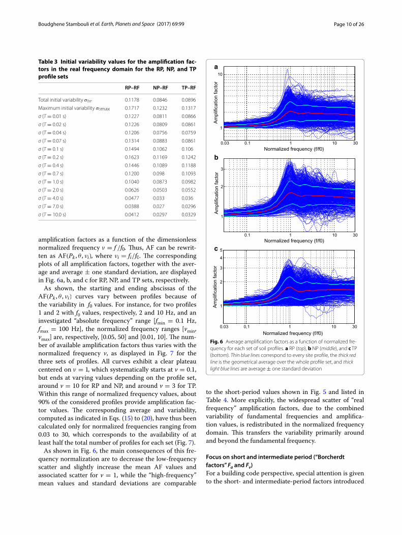
Present implementationFor the present application, the implementation is sepa-rately completed on the three profile sets of RP, NP, and TP. These databases are described in Sect. 2.4.1. The ini-tial set of data to feed the neural network is constituted of nP profiles and their corresponding amplification factors (i.e., AFm(Pk , θ ,Ti) or AFm(Pk , θ , νi)). The input vector consists of a subset of the six site parameters for the RP set, and five site parameters for the NP and TP sets, for which the bedrock velocity is constant. The output con-sists of the calculated AF values for a given period or nor-malized frequency (271 values), and the Borcherdt factors Fa and Fv. This output is labeled AFGRNN(Pk , θ ,Ti) and depends on the number of site proxies used. There is one GRNN model for each scalar output, i.e., 271 scalar mod-els for each period Ti of AFm(Pk , θ ,Ti), 271 scalar models for each normalized frequency νi of AFm(Pk , θ , νi) , one for Fa and one for Fv. All sets of 544 GRNN models are labeled hereafter as xP-yF, according to the correspond-ing profile set (RP, NP, or TP) and the type of frequency values (real or normalized), for instance, RP–RF for real profiles and real frequencies, TP–NF for truncated pro-files and normalized frequencies. All possible combina-tions of input site parameters were considered, so that, as listed in Table 5, 186 sets of GRNN models are obtained: 63 for RP–RF (all possible combinations within six site parameters), 31 for RP–NF, NP–RF, and TP–RF (all pos-sible combinations within five site parameters), and 15 for RP–NF and TP–NF (all possible combinations within four site parameters).

In each case, the networks are trained by dividing the data set into a training set (75%) and a testing set (25%), the elements of which are randomly swapped from one set to another until the width of the Gaussian is robustly

estimated. The Gaussian width is the only free parameter optimized. The full data set is then used to estimate the performance of the GRNN model using various non-independent indicators, such as the coefficient of corre-lation, standard deviation of residuals, and reduction in variance with respect to the initial variability.

ResultsComparisons between original AF and GRNN predictionsOur first goal is to test the ability of the GRNN models using only a limited number of site parameters to sat-isfactorily predict AF values. To achieve that goal, we derived a large number of GRNN models using all possi-ble combinations of input parameters and analyzed their respective performance by comparing the level of the standard deviation of residuals (predicted − actual val-ues) to the initial variability values for each period, i.e., σ0(θ ,Ti), and to the overall variability σ0m(θ) as previ-ously defined.

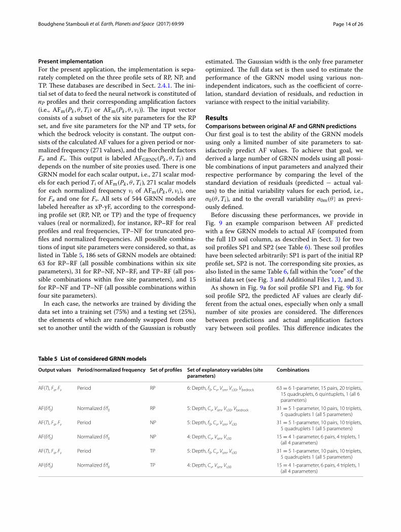
Before discussing these performances, we provide in Fig. 9 an example comparison between AF predicted with a few GRNN models to actual AF (computed from the full 1D soil column, as described in Sect. 3) for two soil profiles SP1 and SP2 (see Table 6). These soil profiles have been selected arbitrarily: SP1 is part of the initial RP profile set, SP2 is not. The corresponding site proxies, as also listed in the same Table 6, fall within the “core” of the initial data set (see Fig. 3 and Additional Files 1, 2, and 3).

As shown in Fig. 9a for soil profile SP1 and Fig. 9b for soil profile SP2, the predicted AF values are clearly dif-ferent from the actual ones, especially when only a small number of site proxies are considered. The differences between predictions and actual amplification factors vary between soil profiles. This difference indicates the

Table 5 List of considered GRNN models

Output values Period/normalized frequency Set of profiles Set of explanatory variables (site parameters)

Combinations

AF(T), Fa, Fv Period RP 6: Depth, f0, Cv, Vsm, Vs30, Vbedrock 63 = 6 1‑parameter, 15 pairs, 20 triplets, 15 quadruplets, 6 quintuplets, 1 (all 6 parameters)

AF(f/f0) Normalized f/f0 RP 5: Depth, Cv, Vsm, Vs30, Vbedrock 31 = 5 1‑parameter, 10 pairs, 10 triplets, 5 quadruplets 1 (all 5 parameters)

AF(T), Fa, Fv Period NP 5: Depth, f0, Cv, Vsm, Vs30 31 = 5 1‑parameter, 10 pairs, 10 triplets, 5 quadruplets 1 (all 5 parameters)

AF(f/f0) Normalized f/f0 NP 4: Depth, Cv, Vsm, Vs30 15 = 4 1‑parameter, 6 pairs, 4 triplets, 1 (all 4 parameters)

AF(T), Fa, Fv Period TP 5: Depth, f0, Cv, Vsm, Vs30 31 = 5 1‑parameter, 10 pairs, 10 triplets, 5 quadruplets 1 (all 5 parameters)

AF(f/f0) Normalized f/f0 TP 4: Depth, Cv, Vsm, Vs30 15 = 4 1‑parameter, 6 pairs, 4 triplets, 1 (all 4 parameters)


importance of analyzing the standard deviation of resid-uals to obtain a statistically meaningful insight into the relative performances of each considered site proxy in controlling the AF.

Analysis of the prediction residualsThe error between prediction and actual values (Eqs. 24–26) is estimated and compared with the initial variabili-ties (Eqs. 18–20).

• For each period and each GRNN model, a period-dependent error term representing the standard deviation of residuals is computed as follows for comparison with the initial variability term σ0(θ ,Ti) (Eq. 18):

• Similarly, in relation to the maximum initial vari-ability σ0max(θ) (see Eq. 19), a “maximum error” is defined as the maximum over all periods/frequencies of εGRNN(θ ,Ti):

• Finally, similar to the overall initial variability term σ0m(θ) (see Eq. 20), an overall error is defined as the average over all periods of the error term:

Examples of the period-dependent error term εGRNN(θ ,Ti) are displayed in Figs. 10, 11 for the real period and normalized frequency domains, respec-tively, together with the initial variabilities, σ(θ ,Ti), of the amplification factor sets. In the former case, the few considered GRNN models are the same as those consid-ered for Fig. 9, i.e., the pairs

(

Cv , f0)

and (

f0,VS30

)

, triplet

(24)

εGRNN(θ ,Ti)

=

√

√

√

√

1

nP

nP∑

k=1

[log (AFGRNN(Pk , θ ,Ti))− log (AFm(Pk , θ ,Ti))]2

(25)εGRNN,max(θ) = MaxTi [εGRNN(θ ,Ti)]

(26)εGRNN,m(θ) =1

nT

nT∑

i=1

εGRNN(θ ,Ti)

0.1 1 101

1.5

2

2.5

3

3.5

4

4.5

Period (s)

Spe

ctra

l am

plifi

catio

n fa

ctor

Target OutputsGRNN Outputs(Inputs:all parameters)GRNN Outputs(Inputs:Cv,Vs30,f0)

GRNN Outputs(Inputs:Cv,f0)

GRNN Outputs(Inputs:Vs30,f0)

GRNN Outputs(Inputs:Vs30)

0.1 1 101

1.5

2

2.5

Period (s)

Spe

ctra

l am

plifi

catio

n fa

ctor

Target OutputsGRNN Outputs(Inputs:all parameters)GRNN Outputs(Inputs:Cv,Vs30,f0)

GRNN Outputs(Inputs:Cv,f0)

GRNN Outputs(Inputs:Vs30,f0)

GRNN Outputs(Inputs:Vs30)

a

b

Fig. 9 Comparison between AF calculated in the 1D analytical model and corresponding GRNN predictions for two example soil profiles. Top soil profile SP1, which is part of the RP set used in the training phase. Bottom soil profile SP2, which is not in the training set

Table 6 Velocity profile and site parameters for the two example soil profiles SP1 (part of the RP set) and SP2 (outside RP set)

Layer # Soil profile 1 Soil profile 2

Thickness hi (m) S-wave velocity Vi (m/s) Thickness hi (m) S-wave velocity Vi (m/s)

1 4 150 2 120

2 10 260 14 510

3 6 420 39 720

4 12 950 108 900

5 40 1470 Bedrock 1000

6 Bedrock 1850

Soil profile Depth (m) f0 (Hz) Vsm (m/s) Cv Vs30 (m/s) Vbedrock (m/s)

SP1 72 3.69 603 12.33 333 1850

SP2 163 1.44 746 8.33 472 1000


(

Cv , f0,VS30

)

, and “all parameter” case, plus three cases of one parameter GRNN, considering individual site prox-ies Cv, VS30 and f0. In the normalized frequency domain case, the parameter “ f0” is replaced with the parameter “Depth,” which is fully independent from the velocity parameters. Figures 10 and 11 exhibit several noticeable features:

• Cv alone allows a significant explanation of the AF, i.e., ε(θ ,Ti) is significantly smaller than σ0(θ ,Ti). It performs even better at short periods than when considering two other site proxies, such as

(

f0,VS30

)

(Fig. 11a). The latter result, however, is not valid for profile sets NP and TP, because of the uniformity of bedrock velocity, which lowers the relative impor-tance of Cv compared to VS30.

• The three-parameter GRNN model, based on (

Cv , f0,VS30

)

, is very powerful to predict actual AF, with residual errors less than 15% of the initial vari-ability. Notably, the “all parameter” GRNN models using “only” five to six parameters provide very sat-isfactory predictions, with residual errors ε(θ ,Ti) less than 5% of the initial variability.

• The largest root-mean-square errors are system-atically found in the short- to intermediate-period range for the real period domain (Fig. 10) and around the fundamental frequency f0 for the normalized fre-quency domain (Fig. 11). This actually corresponds to the frequency range of the largest initial variability.

• The widely used VS30 parameter is found to have a notably good performance only when associated with the fundamental frequency and when bedrock velocity is uniform (Fig. 11b, c). For all other cases (Fig. 10), it performs significantly worse than the sin-gle parameters Cv or f0.

These results are only partial as only seven of the many possible models (for instance, up to 63 for the RP–RF case, see Table 5) are considered. Figure 12 displays the evolu-tion of overall error εm(θ) with the number of proxies for all combinations of site proxies. As listed in Table 5, a given number of explanatory site proxies are associated with many different models. For example, for the RP–RF case, there are 15 possible combinations involving pairs of proxies, 20 involving triplets, and 15 involving quadruplets of site proxies. The zero-proxy value of εm(θ) corresponds to the initial variability σ0m(θ). While it clearly decreases with an increasing number of explanatory site proxies, it also exhibits a significant scatter for a given number of proxies. This indicates that some site proxies perform bet-ter than others in controlling the amplification factor.

Considering the large number of possible combinations (indicated in Table 5), we analyzed the respective per-formances of each proxy by evaluating, for a given num-ber of site proxies, the average value of εm(θ) for all the proxy combinations that involve the considered proxy. For instance, in the RP–RF case, there are 15 possible combinations of pairs of site proxies. Within all these pairs, we characterize the performance of a given proxy (for instance, VS30) using the average value εm(θ) for the five combinations involving that proxy, i.e., the five pairs

0.1 1 100

0.02

0.04

0.06

0.08

0.1

0.12

0.14

0.16

0.18

Period (s)

Stan

dard

dev

iatio

n of

resi

dual

s

All parametersInputs:f0,Vs30,Cv

Inputs:f0,Cv

Inputs:f0,Vs30

Inputs:CvInputs:Vs30Inputs:f0Initial standard deviation

0.1 1 100

0.02

0.04

0.06

0.08

0.1

0.12

0.14

Period (s)

Stan

dard

dev

iatio

n of

resi

dual

s


Inputs:f0,Cv

Inputs:f0,Vs30

Inputs:CvInputs:Vs30

Inputs:f0Initial standard deviation

0.1 1 100

0.02

0.04

0.06

0.08

0.1

0.12

0.14

Period (s)

Stan

dard

dev

iatio

n of

resi

dual

s


Inputs:f0,Cv

Inputs:f0,Vs30

Inputs:CvInputs:Vs30Inputs:f0Initial standard deviation

a

b

c

Fig. 10 Variation in root‑mean‑square error, standard deviation of residuals εGRNN(θ , Ti), for various GRNN models with various sets of input site parameters (indicated with different colors), compared to the initial variability σ0(θ , Ti) (solid green line) for the RP–RF (a, top), NP–RF (b, middle), and TP–RF (c, bottom). Data are displayed as a func‑tion of real period


(VS30,Cv), (VS30,Vbedrock), (

VS30, f0)

, (VS30, Depth) and (VS30,Vsm). This allows us the possibility of identifying the importance of each site proxy using the following quantity:

(27)RSm(θ) = 1−εm(θ)

σm(θ)

where RSm(θ) is the reduction in standard deviation.Another way to measure the importance of each site

proxy is the reduction in variance:

The procedure is repeated for all the possible number of site proxies, which culminates in the curves displayed in Fig. 13 for the three RP, NP, and TP sets. Similar results are obtained for the normalized frequency domain and are provided as additional files.

For the RP and NP sets, one parameter systematically performs better than the others to explain the ampli-fication factor, the velocity contrast Cv (Fig. 13a). This result is not valid for the TP set (Fig. 13c), for which f0 outperforms the other proxies as long as only one or two explanatory site proxies are considered.

(28)RVm(θ) = 1−(εm(θ))

2

(σm(θ))2= RSm(θ)(2− RSm(θ))

0.1 1 10 20 300

0.02

0.04

0.06

0.08

0.1

0.12

0.14

0.16

0.18


Stan

dard

dev

iatio

n of

resi

dual

s All parametersInputs:Depth,Vs30,Cv

Inputs:Depth,CvInputs:Depth,Vs30


Inputs:DepthInitial standard deviation

0.1 1 10 20 300

0.02

0.04

0.06

0.08

0.1

0.12


Stan

dard

dev

iatio

n of

resi

dual

s

All parametersInputs:Depth,Vs30,Cv




0.1 1 10 20 300

0.02

0.04

0.06

0.08

0.1

0.12

0.14


Stan

dard

dev

iatio

n of

resi

dual

s All parametersInputs:Depth,Vs30,Cv




a

b

c

Fig. 11 Variation in root‑mean‑square error, standard deviation of residuals εGRNN(θ , νi), for various GRNN models involving various sets of input parameters (indicated with different colors) compared to the initial variability σ0(θ , νi) for RP–NF (a, top), NP–NF (b, middle) and TP–NF (c, bottom). Data are displayed as a function of normalized frequency ν = f /f0

00.020.040.060.080.1

0.120.14

0 1 2 3 4 5 6 7

Ove

rall

erro

r

Number of explanatory site proxies

Real profiles

00.010.020.030.040.050.060.070.080.09

0 1 2 3 4 5 6

Ove

rall

erro

r


Normalized profiles

00.010.020.030.040.050.060.070.080.090.1

0 1 2 3 4 5 6

Ove

rall

erro

r


Truncated profile

a

b

c

Fig. 12 Progressive reduction in the standard deviation of residuals for all GRNN with the number of explanatory site proxies. As listed in Table 5, a given number of site proxies are associated with many different models, except for the 0 proxy case (initial variability) and “all proxies” case (see text for further details). a RP–RF (top), b NP–RF (middle), and c TP–RF (bottom)


Such results are easily understandable, as the veloc-ity contrast does dominate the impedance contrast that in turn controls the actual amplification for the simple, single-layer case. All other parameters perform simi-larly, however, with a slightly better performance for the fundamental frequency and a slightly worse one for the “whole thickness” parameters Depth and Vsm. As for the widely used VS30 proxy, it performs better than “Depth” and “Vsm” but worse than Cv, f0, and Vbedrock for the RP case, and it is one the two worst proxies (with Vsm) for the

NP and TP sets. Notably, the Depth proxy performs satis-factorily only for constant velocity bedrock.

Therefore, it would be desirable to measure the velocity contrast between bedrock and surface for any site where possible. Unfortunately, such measurements are chal-lenging and/or expensive, and this “optimal” site proxy is almost never available. Therefore, what is the optimal “second choice”? When Cv is not available, it is most often because Vbedrock could not be measured. A careful look at Table 7 indicates that the pair

(

VS30, f0)

provides predic-tion errors similar to Cv alone and that the next relatively efficient site parameter to be considered in combination with others is “Depth.”

Another interesting result is the potential usefulness of considering the normalized frequency space to pre-dict the amplification factor from a few site proxies. A comparison between the performances of real and nor-malized frequency GRNN models (Fig. 13 and Addi-tional File 4, respectively) clearly indicates that RSm(θ) is reduced slightly more when considering f0 directly as an input parameter, rather than simply for normalizing the frequency axis. For instance, RSm(1) is 79% with the parameter pair

(

Cv , f0)

and 93% for the parameter tri-plet

(

Cv , f0,VS30

)

for the RP–RF case, while it is only 38% with the parameter (Cv) and 68% for the parameter pair (Cv ,VS30) for the RP–NF case (see Table 7). The gain in simplicity of the normalized frequency approach, which provides less complex prediction formulae with one fewer parameter, is balanced by a significantly poorer performance.

Variation in Borcherdt factors using GRNNAs indicated previously, site effects can be simply char-acterized with the two Borcherdt factors, Fa and Fv, especially from a regulatory perspective. Therefore, we compute the Borcherdt factors for the GRNN model based the pair of site proxies

(

f0,VS30

)

, which proves to be fairly efficient. Figures 14 and 15 display the depend-ence of these two factors as a function of VS30 and f0. For all cases, this dependence is considered within the 5–95%

0.0010.0020.0030.0040.0050.0060.0070.0080.0090.00

100.00

0 1 2 3 4 5 6 7


Real profiles

Cvf0DepthVsmVs30Vbedrock

0102030405060708090

100

0 1 2 3 4 5 6

Redu

ctio

n of

stan

dard

d

evia

tion

(%)

Redu

ctio

n of

stan

dard

d

evia

tion

(%)

Redu

ctio

n of

stan

dard

d

evia

tion

(%)


Normalized profiles

Cvf0DepthVsmVs30

0102030405060708090

100

0 1 2 3 4 5 6


Truncated profiles

Cvf0DepthVsmVs30

a

b

c

Fig. 13 Reduction in standard deviation RSm as performance indica‑tor for various site proxies (different curves) for RP–RF (a, top), NP–RF (b, middle), and TP–RF (c, bottom)

Table 7 Standard deviation of model residuals for various GRNN models implying the initial, actual frequency amplifica-tion factors (RP, NP, TP cases, last three columns) for various combinations of site parameters

Number of parameters Considered site parameters Error (RP) Error (NP) Error (TP)

All (6) Depth + f0 + Vsm + Cv +Vs30 + Vbedrock 0.0011 0.0032 0.0053

3 (best triplet) f0 + Cv + Vs30 0.0079 0.0079 0.0118

2 (best pair) f0 + Cv 0.0251 0.0233 0.0278

2 (convenient pair) f0 + Vs30 0.0782 0.0382 0.0339

1 (best) Cv 0.0725 0.0652 0.0622

1 (usual) Vs30 0.1038 0.0715 0.0733

1 f0 0.099 0.0678 0.0563

Overall initial variability term σm(θ) 0.1178 0.0846 0.0896


f 0 (hz)

fa

200 244.56 299.06 365.71 447.21 546.87 668.74 817.76 1 000

0.8

1.20

1.81

2.72

4.10

6.17

9.30

141.2

1.4

1.6

1.8

2

2.2

2.4

2.6

2.8

Vs30 (m/s)

Vs30 (m/s)

f 0 (hz)

fa

150 176.45 207.56 244.17 287.22 337.87 397.46 467.55 550

0.8

1.2

1.81

2.72

4.10

6.17

9.32

141.2

1.4

1.6

1.8

2

2.2

2.4

Vs30 (m/s)

f 0 (hz)

fa

150 176.45 207.56 244.17 287.22 337.87 397.46 467.55 550

0.8

1.2

1.81

2.72

4.10

6.17

9.32

14

1.2

1.4

1.6

1.8

2

2.2

a

b

c

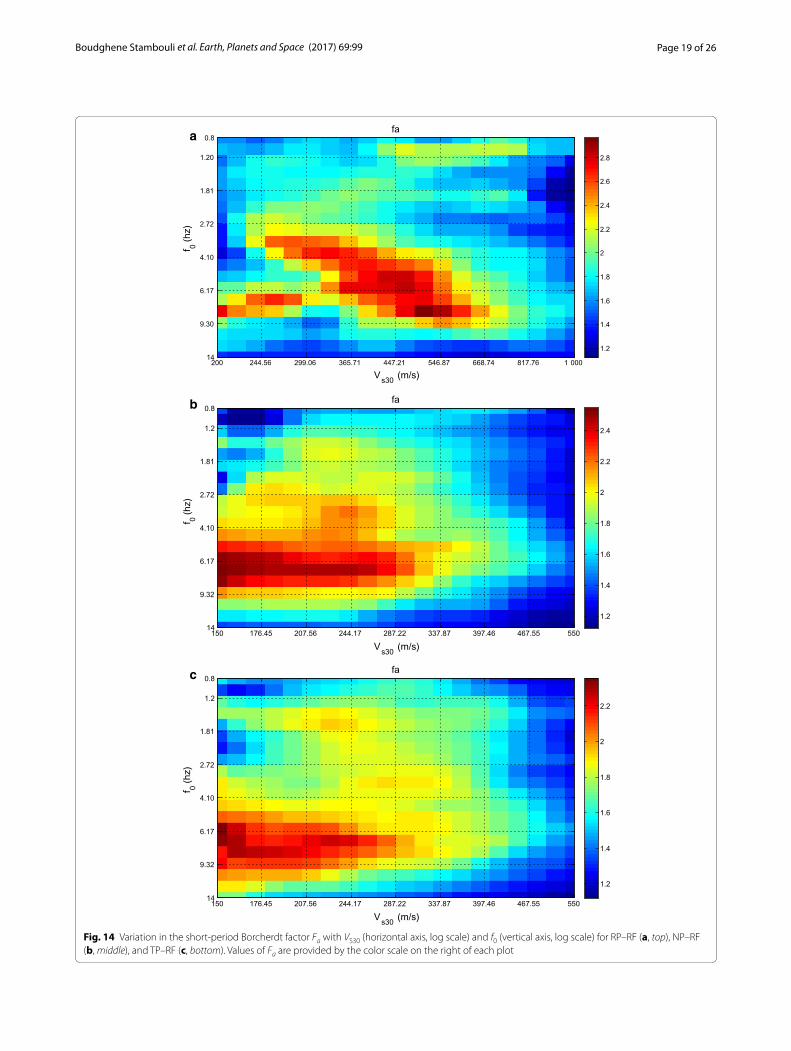
Fig. 14 Variation in the short‑period Borcherdt factor Fa with VS30 (horizontal axis, log scale) and f0 (vertical axis, log scale) for RP–RF (a, top), NP–RF (b, middle), and TP–RF (c, bottom). Values of Fa are provided by the color scale on the right of each plot


Vs30 (m/s)

f 0 (hz)

fv

200 244.56 299.06 365.71 447.21 546.87 668.74 817.76 1 000

0.8

1.2

1.81

2.72

4.10

6.17

9.30

14

1.2

1.4

1.6

1.8

2

2.2

Vs30 (m/s)

f 0 (hz)

fv

150 176.45 207.56 244.17 287.22 337.87 397.46 467.55 550

0.8

1.2

1.81

2.72

4.10

6.17

9.32

14

1.2

1.4

1.6

1.8

2

2.2

2.4

Vs30 (m/s)

f 0 (hz)

fv

150 176.45 207.56 244.17 287.22 337.87 397.46 467.55 550

0.8

1.2

1.81

2.72

4.10

6.17

9.32

14

1.2

1.4

1.6

1.8

2

2.2

2.4

a

b

c

Fig. 15 Variation in the mid‑period Borcherdt factor Fv with VS30 (horizontal axis, log scale) and f0 (vertical axis, log scale) for RP–RF (a, top), NP–RF (b, middle), and TP–RF (c, bottom). Values of Fv are provided by the color scale on the right of each plot


fractile range of each considered explanatory parameter. The [0.8, 14 Hz] interval is considered for f0 in all cases, even though it would be possible to consider higher fre-quencies for the TP case. The considered VS30 interval is [200, 1000 m/s] for the RP case and [150, 550 m/s] for the NP and TP cases.

The corresponding distribution of soil profiles for any pair of site proxies

(

f0,VS30

)

is mapped in Fig. 16 for pro-file sets of RP, NP, and TP. This distribution is rather uni-form in the two latter cases, while there is a lack of data in the RP set in the lower left and upper right corners. Therefore, the RP–RF model is poorly constrained for high-frequency, low-velocity sites (typically f0 > 5 Hz and VS30 < 350 m/s) and for low-frequency, high-veloc-ity sites (typically f0 < 2 Hz and VS30 > 600 m/s).

The behavior of Fa and Fv with f0 and VS30 is expressed with the following explicit equation associated with the GRNN models:

where wj are the weights of each training data, estimated from their Euclidian distance in the (log(f0), log(VS30)) plane (x1 = log

(

f0)

and x2 = log(VS30))

(29)log (Fa) =Q∑

j=1

(

log(

Fa,j)

wj

)

/

Q∑

j=1

wj

(30)wj = exp

−

�

b

�

�

�

log�

f0�

− log(f0,j)�2 +

�

log�

VS30 − log(VS30,j)��2

�

.

�2

f0 below 1.5–2 Hz, VS30 below 200 m/s (Fig. 15). Con-versely, Fv remains small (below 1.4) for high-frequency sites ( f0 beyond 4 Hz) for all values of VS30. For RP, it may remain significant (between 1.4 and 1.6) for stiff sites (VS30 >400 m/s) and low frequency when the bedrock is deep and hard enough for the fundamental frequency to remain below 2 Hz. However, for NP and TP it is lower than 1.4 when VS30 exceeds 350 m/s.

Which among the RP–RF, NF–RF, and TP–RF rela-tionships should be used for practical purposes? It should first be reminded that the present study only addresses the linear case as a preliminary, feasibility stage. This may explain for the relatively limited Fv val-ues, which are often smaller than the Fa values. However, to obtain first-order estimates of Fa and Fv values for the linear response of a given site, the first step is to approxi-mately identify the stiffness of underlying bedrock. For very hard bedrock, with S-wave velocities exceeding 1.2–1.5 km/s, it is better to select the RP–RF relation-ships. For bedrock that may be assumed to be close to a “standard” bedrock, with a S-wave velocity between 600 and 1000 m/s, and when VS30 value is below 550 m/s, it is probably preferable to select the NP–RF or TP–RF relationships. As shown in Fig. 16 (and Table 2), the

and similar relationships for Fv.The optimal b value is derived during the training

phase and found to be equal to 16.65.An Excel file is provided as an additional file for the

practical use of these equations.Generally, the short-period amplification factor Fa

(Fig. 14) reaches the highest values for sites with inter-mediate to high fundamental frequency and low veloci-ties at shallow depth. The maximum values exceed 2.5 for all cases, but correspond to slightly different

(

f0,VS30

)

combinations. Large Fa are found for the RP setup to VS30 values of 550 m/s (and corresponding fundamental fre-quencies around 6–9 Hz), while for the NP and TP sets, they are restricted to VS30 values below 300 m/s. Such dif-ferences are related to the possibility of high amplitude resonance when a thin layer of stiff soil is underlain by very hard rock, a situation that is quite frequent in real profiles. It is impossible in normalized or truncated pro-files because of the velocity reduction imposed by the 800 m/s bedrock condition.

In parallel, the intermediate-period amplification factor Fv is found, as expected, to reach its highest val-ues, above 2, for low-frequency and low-velocity sites:

relationship may be considered reliable for the whole rectangular area described by the 5–95% fractile range of the two parameters for the NP and TP cases. In contrast, the RP model is poorly constrained for high-frequency, low-velocity sites and for low-frequency, high-velocity sites.

Finally, for the AF values, all possible combinations of site parameters are also considered, and associ-ated GRNN models are derived and analyzed. The per-formances of some are listed in Tables 8, 9, 10, and the average performance of each considered site proxy is dis-played in Fig. 17, similar to in Fig. 13, for the two param-eters Fa and Fv.

As expected from previous results, one parameter per-forms almost systematically better than the others to explain the amplification factors, the velocity contrast Cv . However, it is superseded by the fundamental frequency for predicting Fv values in all three RP, NP, and TP cases, and f0 proves to be a very relevant parameter for inter-mediate- to long-period amplification. The widely used VS30 proxy performs better than the fundamental fre-quency f0 only for Fa and in the NP case, and the perfor-mance gain is only slight.


200 244.56 299.06 365.71 447.21 546.87 668.74 817.76 1000

0.8

1.20

1.81

2.72

4.10

6.17

9.30

14

Vs30 (m/s)

f 0 (hz)

150 176,45 207,56 244,17 287.22 337.87 397.46 467.55 550

0.8

1.2

1.81

2.72

4.10

6.17

9.30

14

Vs30 (m/s)

f 0 (hz)

150 176.45 207.56 244.17 287.22 337.87 397.46 467.55 550

0.8

1.2

1.81

2.72

4.10

6.17

9.30

14

Vs30 (m/s)

f 0 (hz)

a

b

c

Fig. 16 Distribution of the initial data in the (VS30, f0) plane (log–log axis) for profile sets RP (a, top), NP (b, middle), and TP (c, bottom)

ConclusionsThe present study was a numerical investigation aim-ing at identifying the key parameters controlling 1D site response, starting with the linear domain as the first stage. For 858 soil columns corresponding to measured, real sites profiles from Japan, the USA, and Europe, the 1D linear (viscoelastic) response was computed for ver-tically incident plane waves and a representative set of

real input accelerograms spanning a wide range of peak frequencies. The geometric averages of the correspond-ing amplifications were derived from the ratio of surface to input acceleration response spectra, both in terms of frequency-dependent amplification factors AF(f ) and in terms of “summary” short- and mid-period ampli-fication factors Fa and Fv, averaged over period ranges [0.1 s, 0.2 s] and [0.75 s, 1.5 s], respectively. Generalized regression neural network (GRNN) models were used to investigate the relationships between these amplifica-tion factors and several “usual” site proxies, i.e., VS30, f0 , sediment thickness, corresponding harmonic average sediment velocity, maximum velocity contrast, and bed-rock velocity. Since real profiles exhibit a large site-to-site variability in bedrock velocity, two other sets of profiles with a constant bedrock velocity set to 800 m/s were con-sidered. A common scaling was first applied to velocity and thickness values to normalize the real profiles to a uniform bedrock velocity of 800 m/s (without changing the transfer functions). The same real profiles were also truncated at the depth where their S-wave velocity first exceeded 800 m/s. GRNN models were then developed for these two additional sets of profiles. Many GRNN models were considered in each case, with all possible combinations of site proxies. This provided a mecha-nism for comparing the performances of every proxy to explain (and predict) site amplification.

The results showed that the key characteristics of the frequency-dependent AF may be satisfactorily repro-duced with a limited number of site proxies. The best performing site parameter is the overall impedance con-trast between bedrock velocity and minimum surface velocity. Because it is one of the most difficult and expen-sive parameters to measure, especially for thick deposits, other more convenient parameters are preferred, among them, the couple

(

VS30, f0)

reduced the variance of resid-uals by at least 60%. From a code perspective, equations and plots were provided describing the dependence of the short- and mid-period amplification factors Fa and Fv on these two parameters. Fa reached its highest value for sites presenting simultaneously low velocities and high f0 values (i.e., thin, soft sites), while the largest values of Fa corresponded to low velocities and low f0 values.

These results open the way for improvements in site classification with a physical relationship between site proxies and site amplification. However, this work is only a first step, and the present results should be comple-mented with further investigations.

• First, the set of considered soil profiles is dominated by KiK-net sites, which are rather stiff. Although this bias was somewhat corrected with the set of “nor-


malized profiles” or “truncated profiles,” it is not fully satisfactory because the normalization procedure also included a depth scaling to maintain unchanged

frequencies. Adding softer sites would extend the applicability range of the results to softer and thicker sites.

Table 8 Evolution of the standard deviation of residuals for various GRNN models predicting Fa and Fv in the RP–RF case

Number of parameters Explanatory parameters Fa Fv

Standard deviation of residuals

Variance reduction Standard deviation of residuals

Variance reduction

All (6) Depth + f0 + Vsm + Cv + Vs30 + Vbed‑

rock

0.0020 99.9% 0.00023 99.9%

3 (best triplet) f0 + Cv + Vs30 0.0094 99.6% 0.0067 99.5%

2 (best pair) f0 + Cv 0.0349 94.9% 0.0173 97.0%

2 (convenient pair) f0 + Vs30 0.1083 50.7% 0.0515 73.2%

1 (best for Fa) Cv 0.0878 67.6% 0.0786 37.6%

1 (best for Fv) f0 0.1355 22.9% 0.0661 55.9%

1 (usual) Vs30 0.1419 15.4% 0.0752 42.9%

Initial σ 0.1543 0.0995

Table 9 Evolution of the standard deviation of residuals for various GRNN models predicting Fa and Fv in the NP–RF case

Normalized profiles Fa Fv

Number of param-eters

Explanatory parameters Standard deviation of residuals


Variance reduction

All (5) Depth + f0 + Vsm + Cv + Vs30 0.0055 99.74% 0.0011 99.98%


2 (best pair for Fa) f0 + Cv 0.0318 91.43% 0.0172 95.7%


1 (best for Fa) Cv 0.0783 48.02% 0.0733 21.8%

1 (best for Fv) f0 0.0944 24.44% 0.048 66.4%

1 (usual) Vs30 0.0926 27.3% 0.0709 26.8%

Initial σ 0.1086 0.0829

Table 10 Evolution of the standard deviation of residuals for various GRNN models predicting Fa and Fv in the TP–RF case

Truncated profiles Fa Fv

Number of param-eters

Explanatory parameters Standard deviation of residuals


Variance reduction

All 5 Depth + f0 + Vsmn + Cv + Vs30 0.0095 99.28% 0.0017 99.97%


2 (best pair for Fa) f0 + Cv 0.0375 88.8% 0.0229 93.9%


1 (best, Fa) Cv 0.0734 57.05% 0.0736 37.9%

1 (best, Fv) f0 0.0764 53.47% 0.0428 79%

1 (usual) Vs30 0.0925 31.4% 0.0777 30.8%

Initial σ 0.112 0.0934


• Second, these results are limited to the linear case. An important next step will be to consider nonlinear site responses. Assigning nonlinear characteristics to different layers of each soil pro-

file (information that is presently unavailable) and adding at least one explanatory variable in the input layer, related to the loading level, will be required.

0102030405060708090

100

0 1 2 3 4 5 6Redu

ctio

n of

stan

dard

dev

iatio

n (%

)


Real profiles, sigma reduction for Fa

Cv

f0

Depth

Vsm

Vs30

Vbedrock 0102030405060708090

100

0 1 2 3 4 5 6Redu

ctio

n of

stan

dard

dev

iatio

n (%

)


Real profiles, sigma reduction for Fv

Cv

f0

Depth

Vsm

Vs30

Vbedrock

0

10

20

30

40

50

60

70

80

90

100

0 1 2 3 4 5

Redu

ctio

n of

stan

dard

dev

iatio

n (%

)


normalized profiles,sigma reduction for Fa

Cv

f0

Depth

Vsm

Vs30

0

10

20

30

40

50

60

70

80

90

100

0 1 2 3 4 5

Redu

ctio

n of

stan

dard

dev

iatio

n (%

)


normalized profiles, sigma reduction for Fv

Cv

f0

Depth

Vsm

Vs30

0

20

40

60

80

100

0 1 2 3 4 5Redu

ctio

n of

stan

dard

dev

iatio

n (%

)


Truncated profiles,sigma reduction for Fa

Cv

f0

Depth

Vsm

Vs300

20

40

60

80

100

0 1 2 3 4 5

Redu

ctio

n of

stan

dard

dev

iatio

n (%

)


Truncated profiles, sigma reduction for Fv

Cv

f0

Depth

Vsm

Vs30

a1 a2

b1 b2

c1 c2

Fig. 17 Performance indicators for Borcherdt factors prediction models based on the reduction in the standard deviation of residuals RSm for vari‑ous site proxies (different curves) for RP–RF (a, top), NP–RF (b, middle), and TP–RF (c, bottom). The left column (1) corresponds to Fa models, and the right one (2) corresponds to Fv models. The display is similar to that presented in Fig. 13


AbbreviationsAF: amplification factor (ratio of site to “reference rock” acceleration response spectrum with 5% damping); Cv: velocity contrast between bedrock and the softest layers, which is generally at the surface, but not systematically; Depth: thickness down to the deepest (and hardest) geological unit; f0: resonance frequency; Fa: amplification factor at short period (computed as the geo‑metrical mean of AF for periods equally spaced on a logarithmic axis in the range [0.1 s, 0.2 s]); Fv: amplification factor at mid‑period (computed as the geometrical mean of AF for periods equally spaced on a logarithmic axis in the range [0.75 s, 1.5 s]); GMPEs: ground motion prediction equations; GRNN: generalized regression neural network; hi: thickness of layer i; Mw: moment magnitude; RP: real profiles; NP: normalized profiles; TP: truncated profiles; NF: normalized frequency; RF: real frequency; PGA: peak ground acceleration; PSA: pseudo acceleration spectrum; Qi: quality factor for layer i; R2: coefficient of determination; SA(T )b: 5% response spectra at the outcropping reference bedrock; SA(T )s: 5% response spectra at the site surface; Vi: shear wave veloc‑ity for layer i; VBedrock: shear wave velocity of bedrock; VS30: harmonic average of the shear wave velocity over the topmost 30 m; Vsm: harmonic average of shear wave velocity over the total soil column thickness; ξi: damping of layer i; ρi: mass density for layer i.

Authors’ contributionsMost scientific and technical work was conducted by the first author (Ahmed Boudghene Stambouli), under the scientific supervision of the three other coauthors. The preparation and editing of the manuscript were shared between the three first authors. All authors read and approved the final manuscript.

Author details1 Risk Assessment and Management Laboratory (RISAM), Faculté de Technolo‑gie, Université Abou Bekr Belkaïd, BP 230‑13048, Tlemcen, Algeria. 2 Institut de Sciences de la Terre (ISTerre), Maison des Géosciences, Université Grenoble‑Alpes, IFSTTAR, Bâtiment OSUG C, CS 40700, 38058 Grenoble Cedex 9, France.

AcknowledgementsThis work was partially supported by the project: “Prédiction du mouvement sismique et estimation du risque sismique lié aux effets de site” 13MDU901 Tassili CMEP between Universities of Tlemcen (Algeria) and Grenoble (France). The authors wish to express their acknowledgment for this support. They wish also to acknowledge the contribution of C. Cornou from IsTerre (U. Grenoble) and D. Boore from the USA Geologic Survey who provided data for the 858 soil profiles. We also thank Dr. Sanjay Singh Bora and an anonymous reviewer for their careful reading and helpful comments and suggestions that have greatly contributed to clarify several issues and improved the final version. The final editing largely benefitted from the Earth, Planets, and Space journal services.

Competing interestsThe authors declare they have no competing interests.

Additional files

Additional file 1. Distribution of the site parameters for the “real profiles” (RP) set

Additional file 2. Distribution of the site parameters for the “normalized Profiles”

Additional file 3. Distribution of the site parameters for the “truncated profiles”

Additional file 4. Analog to Fig. 13 for the normalized frequency domain: (reduction in standard deviation RSm) for the various site proxies (different curves) for RP–NF (a, top), NP–NF (b, middle), and TP–NF (c, bottom)

Additional file 5. Excel sheet to estimate the short‑ and mid‑period amplification factors Fa and Fv based on VS30 and f0 values for RP–RF

Availability of data and materialsThe RP profile set was originally compiled by C. Cornou (Salameh 2016) and consists of about 600 Japanese KiK‑net sites, more than 200 sites from the USA, made available by D. Boore (http://quake.usgs.gov/~boore), and 22 European sites measured during the NERIES project (Di Giulio et al. 2012). The KiK‑net velocity profiles were directly obtained from http://www.kyoshin.bosai.go.jp and consist of surface‑to‑downhole measurements of S‑ and P‑wave velocities.

Publisher’s NoteSpringer Nature remains neutral with regard to jurisdictional claims in pub‑lished maps and institutional affiliations.

Received: 28 November 2016 Accepted: 14 July 2017

ReferencesAbrahamson N, Atkinson G, Boore D, Bozorgnia Y, Campbell K, Chiou B, Idriss

I, Silva W, Youngs R (2008) Comparisons of the NGA ground‑motion rela‑tions. Earthq Spectra 24(1):45–66

Aki K, Richards PG (1980) Quantitative seismology, theory and methods, vol 1. WH Freeman & Co., New York

Akkar S, Sandıkkaya MA, Şenyurt M, Sisi AA, Ay BÖ, Traversa P, Godey S (2014) Reference database for seismic ground‑motion in Europe (RESORCE). Bull Earthq Eng 12(1):311–339

Almakari M, Régnier J, Salameh C, Cadet H, Bard PY, Lopez‑Caballero F, Cornou C (2016) Modulation of weak motion site transfer functions by non‑linear behavior: a statistical comparison of 1D numerical simulation with KiK‑net data. In: Proceedings of the 5th IASPEI/IAEE international symposium: effects of surface geology on seismic motion, Taipei, August 15–17 Paper P101C, 14 pp

Ancheta TD, Darragh RB, Stewart JP, Seyhan E, Silva WJ, Chiou BS‑J, Wooddell KE, Graves RW, Kottke AR, Boore DM, Kishida T, Donahue JL (2014) NGA‑West 2 database. Earthq Spectra 30:989–1005

Anderson JG, Bodin P, Brune JN, Prince J, Singh SK, Quaas R, Onate M (1986) () Strong ground motion from the Michoacan, Mexico, earthquake. Science 233(1043):9

Bard P‑Y, Campillo M, Chavez‑Garcia FJ, Sanchez‑Sesma FJ (1988) The Mexico earthquake of September 19, 1985—a theoretical investigation of large‑ and small‑scale amplification effects in the Mexico City Valley. Earthq Spectra 4(3):609–633. doi:10.1193/1.1585493

Bardet JP, Ichii K, Lin CH (2000) EERA: a computer program for equivalent‑linear earthquake site response analyses of layered soil deposits. University of Southern California, Department of Civil Engineering

Biro Y, Renault P (2012) Importance and impact of host‐to‐target conversions for ground motion prediction equations in PSHA. In: Proceedings of the 15th world conference on earthquake engineering, pp 24–28

Bora SS, Scherbaum F, Kuehn N, Stafford P, Edwards B (2015) Development of a response spectral ground‑motion prediction equation (GMPE) for seismic‑hazard analysis from empirical fourier spectral and duration models. Bull Seism Soc Am 105(4):2192–2218

Bora SS, Scherbaum F, Kuehn N, Stafford P (2016) On the relationship between fourier and response spectra: implications for the adjustment of empiri‑cal ground‑motion prediction equations (GMPEs). Bull Seism Soc Am 106(3):1235–1253

Borcherdt RD (1994) Estimates of site dependent response spectra for design (methodology and justification). Earthq Spectra 10:617–653

Borcherdt RD (2002) Empirical evidence for acceleration‑dependent amplifica‑tion factors. Bull Seism Soc Am 92(2):761–782

Cadet H, Bard P‑Y, Duval A‑M, Bertrand E (2012) Site effect assessment using KiK‑net data—part 2—site amplification prediction equation (SAPE) based on f0 and Vsz. Bull Earthq Eng 10:451–489

Castellaro S, Mulargia F, Rossi PM (2008) Vs30: proxy for seismic amplification? Seism Res Lett 79:540–543

http://dx.doi.org/10.1186/s40623-017-0686-3

http://dx.doi.org/10.1186/s40623-017-0686-3

http://dx.doi.org/10.1186/s40623-017-0686-3

http://dx.doi.org/10.1186/s40623-017-0686-3

http://dx.doi.org/10.1186/s40623-017-0686-3

http://quake.usgs.gov/%7eboore

http://www.kyoshin.bosai.go.jp

http://www.kyoshin.bosai.go.jp

http://dx.doi.org/10.1193/1.1585493


Chávez‑García FJ, Bard PY (1994) Site effects in Mexico City eight years after the September 1985 Michoacan earthquakes. Soil Dyn Earthq Eng 13(4):229–247

Cigizoglu HK, Alp M (2005) Generalized regression neural network in model‑ling river sediment yield. Adv Eng Softw 37:63–68

Cruz‑Atienza VM, Tago J, Sanabria‑Gómez JD, Chaljub E, Etienne V, Virieux J, Quintanar L (2016) Long duration of ground motion in the paradigmatic valley of Mexico. Sci Rep 6:38807

Derras B, Bard PY, Cotton F, Bekkouche A (2012) Adapting the neural network approach to PGA prediction: an example based on the KiK‑net data. Bull Seism Soc Am 102(4):1446–1461

Derras B, Bard PY, Cotton F (2014) Towards fully data driven ground‑motion prediction models for Europe. Bull Earthq Eng 12(1):495–516. doi:10.1007/s10518‑013‑9481‑0

Derras B, Bard P‑Y, Cotton F (2016) Site‑conditions proxies, ground‑motion variability and data‑driven GMPEs. Insights from NGA‑West 2 and RES‑ORCE datasets. Earthq Spectra 32(4):2027–2056

Di Giulio G, Savvaidis A, Ohrnberger M, Wathelet M, Cornou C, Knapmeyer‑Endrun B, Renalier F, Theodoulidis N, Bard P‑Y (2012) Exploring the model space and ranking a best class of models in surface‑wave dispersion inversion: application at European strong motion sites. Geophysics 77:B147

Dickenson SE, Seed RB (1996) Nonlinear dynamic response of soft and deep cohesive soil deposits. In: Proceedings of the international workshop on site response subjected to strong earthquake motions, vol 2, pp 67–81

Dobry R, Oweis I, Urzua A (1976) Simplified procedures for estimating the fundamental period of a soil profile. Bull Seism Soc Am 66(4):1293–1321

Dobry R, Borcherdt RD, Crouse CB, Idriss IM, Joyner WN, Martin GR, Power MS, Rinne EE, Seed RB (2000) New Site coefficients and site classification system used in recent building seismic code provisions. Earthq Spectra 16(1):41–67

Douglas J, Akkar S, Ameri G, Bard P‑Y, Bindi D, Bommer JJ, Singh Bora S, Cotton F, Derras B, Hermkes M, Kuehn NM, Luzi L, Massa M, Pacor F, Riggelsen C, Sandıkkaya MA, Scherbaum F, Stafford PJ, Traversa P (2014) Comparisons among the five ground‑motion models developed using RESORCE for the prediction of response spectral accelerations due to earthquakes in Europe and the Middle East. Bull Earthq Eng 12(1):341–358. doi:10.1007/s10518‑013‑9522‑8

EC8 Eurocode 8 (2004). Design of structures for earthquake resistance—Part 1: general rules, seismic actions and rules for buildings. European Commit‑tee for Standardization (CEN), EN 1998‑1, eurocodes.jrc.eceuropa.eu/. Last accessed Feb 2016

Esteva L (1988) The Mexico earthquake of September 19, 1985—conse‑quences, lessons, and impact on research and practice. Earthq Spectra 4:413–426

Fukushima Y, Gariel JC, Tanaka R (1995) Site‑dependent attenuation relations of seismic motion parameters at depth using borehole data. Bull Seism Soc Am 85(6):1790–1804

Ghaboussi J, Lin CCJ (1998) New method of generating spectrum compatible accelerograms using neural networks. Earthq Eng Struct Dyn 27:377–396

Giacinto G, Paolucci R, Roli F (1997) Application of neural networks and statisti‑cal pattern recognition algorithms to earthquake risk evaluation. Pattern Rec Lett 18:1353–1362

Gregor N, Abrahamson NA, Atkinson GM, Boore DM, Bozorgnia Y, Campbell KW, Brian Chiou BS‑J, Idriss IM, Kamai R, Seyhan E, Silva W, Stewart JP, Youngs R (2014) Comparison of NGA‑West2 GMPEs. Earthq Spectra 30(3):1179–1197

Hall JF, Beck JL (1986) Structural damage in Mexico City. Geophys Res Lett 13(6):589–592

Hannan SA, Manza RR, Ramteke RJ (2010) Generalized regression neural network and radial basis function for heart disease diagnosis. Int J Comp App 7(13):7–13

Hashash YMA, Groholski DR, Phillips CA, Park D, Musgrove M (2012) DEEPSOIL 5.1, user manual and tutorial. Department of Civil and Environmental Engineering, University of Illinois at Urbana‑Champaign

Haskell NA (1953) The dispersion of surface waves on multilayered media. Bull Seism Soc Am 43:17–34

IBC (2012) International Building Code 2012 Edition, ISBN 978‑1‑60983‑039‑7, International Code Council, Washington. https://archive.org/details/gov.law.icc.ibc.2012. Last accessed Nov 2016

Kawase H, Aki K (1989) A study on the response of a soft soil basin for incident S, P, and Rayleigh waves with special reference to the long duration observed in Mexico City. Bull Seism Soc Am 79:1361–1382

Kim B, Lee DW, Parka KY, Choi SR, Choi S (2004) Prediction of plasma etching using a randomized generalized regression neural network. Vacuum 76:37–43

Kramer SL (1996) Geotechnical earthquake engineering. Pearson Education India, New Delhi

Lin CCJ, Ghaboussi J (2001) Generating multiple spectrum compatible accelerograms using stochastic neural networks. Earthq Eng Struct Dyn 30:1021–1042

Luzi L, Puglia R, Pacor F, Gallipoli MR, Bindi D, Mucciarelli M (2011) Proposal for a soil classification based on parameters alternative or complementary to Vs, 30. Bull Earthq Eng 9(6):1877–1898

Martin GR, Dobry R (1994) Earthquake site response and seismic code provi‑sions. NCEER Bull 8(4):1–6

Paolucci R, Colli P, Giacinto G (2000) Assessment of seismic site effect in 2‑D alluvial valleys using neural networks. Earthq Spectra 16:661–680

Pitilakis KD, Makra KA, Raptakis DG (2001) 2D vs 3D site effects with potential applications to seismic norms: the case of EUROSEISTEST and Thessa‑loniki. In: Proceedings of the XVth ICSMGE, Istanbul, pp 123–133

Pitilakis K, Riga E, Anastasiadis A (2012) Design spectra and amplification fac‑tors for Eurocode 8. Bull Earthq Eng 10(5):1377–1400

Pitilakis K, Riga E, Anastasiadis A (2013) New code site classification, amplifica‑tion factors and normalized response spectra based on a worldwide ground‑motion database. Bull Earthq Eng 11(4):925–966

Renault PLA, Abrahamson NA, Bard P‑Y, Fäh D, Pecker A, Studer J (2014) PEGA‑SOS Refinement Project, volume 5, SP3 ‑ Site Response Characterization, 672 pp. Available from http://www.swissnuclear.ch/de/downloads.html. ©2013‑2015 Swissnuclear, Olten

Rodriguez‑Marek A, Bray JD, Abrahamson NA (2001) An empirical geotechnical seismic site response procedure. Earthq Spectra 17(1):65–87

Romo MP, Jaime A, Resendiz D (1988) General soil conditions and clay proper‑ties in the Valley of Mexico. Earthq Spectra 4:731–752

Salameh C (2016) Ambient vibrations, spectral contents and seismic damage: a new approach adapted to urban scale. Application to Beirut (Lebanon). PhD thesis, University Grenoble‑Alpes, France, defended on June 21, 2016 (284 pp, in English)

Salameh C, Bard P‑Y, Guillier B, Harb J, Cornou C, Gérard J, Almakari M (2017) Using ambient vibration measurements for risk assessment at an urban scale: from numerical proof of concept to Beirut case study (Lebanon). Earth Plan Space 69:60. doi:10.1186/s40623‑017‑0641‑3

Sanchez‑Sesma F, Chavez‑Perez S, Suarez M, Bravo MA, Perez‑Rocha LE (1988) On the seismic response of the Valley of Mexico. Earthq Spectra 4:569–589

Schnabel PB, Lysmer J, Seed HB (1973). SHAKE–a computer program for earth‑quake response analysis of horizontally layered sites, Report No, EERC 72 12, Earthquake Engineering Research Center, University of California, Berkeley

Seed HB, Romo MP, Sun JI, Jaime A, Lysmer J (1988) Relationships between soil conditions and earthquake ground motions. Earthq Spectra 4:687–729

Singh SK, Ordaz M (1993) On the Origin of long coda observed in the lake‑bed strong‑motion records of Mexico City. Bull Seism Soc Am 83:1298–1306

Singh SK, Lermo J, Dominguez T, Ordaz M, Espinosa JM, Mena E, Quaas R (1988a) The Mexico earthquake of September 19, 1985—a study of amplification of seismic waves in the valley of Mexico with respect to a hill zone site. Earthq Spectra 4(4):653–673

Singh SK, Mena EA, Castro R (1988b) Some aspects of source characteristics of the 19 September 1985 Michoacan earthquake and ground motion amplification in and near Mexico City from strong motion data. Bull Seism Soc Am 78(2):451–477

Specht DF (1991) A general regression neural network. IEEE Trans Neural Netw 2(6):568–576

Thomson WT (1950) Transmission of elastic waves through a stratified solid medium. J Appl Phys 21:89–93

Uniform Building Code (1997) Structural engineering design provisions. In: International conference of building officials, vol 2

Wasserman PD (1993) Advanced methods in neural computing. Wiley, New York

http://dx.doi.org/10.1007/s10518-013-9481-0

http://dx.doi.org/10.1007/s10518-013-9522-8

http://dx.doi.org/10.1007/s10518-013-9522-8

https://archive.org/details/gov.law.icc.ibc.2012

https://archive.org/details/gov.law.icc.ibc.2012

http://www.swissnuclear.ch/de/downloads.html

http://dx.doi.org/10.1186/s40623-017-0641-3

OpAccess Derivinglamplikcationlfactorsl ... · Derivinglamplikcationlfactorsl...

Documents

Transcript of OpAccess Derivinglamplikcationlfactorsl ... · Derivinglamplikcationlfactorsl...