Universiteit Gent

Faculteit Ingenieurswetenschappen

Vakgroep

Mechanica van Stroming, Warmte en Verbranding

Voorzitter: Prof. Dr. Ir. R. SIERENS

Ontwikkeling van een simulatieprogramma voor verdampers

door

Dominic SMITH

Promotor: Prof. Dr. Ir. M. DE PAEPE

Begeleiders: Ir. H. CANIÈRE en Ir. C. T’JOEN

Scriptie ingediend tot het behalen van de academische graad van burgerlijk werktuigkundig-elektrotechnisch ingenieur

Academiejaar 2006-2007

ACKNOWLEDGEMENTS

I would like to thank Prof. Dr. Ir. M. De Paepe, Ir. H. Canière and Ir. C. T’Joen for their supervision and guidance during this project.

A special thanks to all the people who helped me through this challenge with their cooperation and friendship.

De auteur geeft de toelating deze scriptie voor consultatie beschikbaar te stellen en delen van de scriptie te kopiëren voor persoonlijk gebruik. Elk ander gebruik valt onder de beperkingen van het auteursrecht, in het bijzonder met betrekking tot de verplichting de bron uitdrukkelijk te vermelden bij het aanhalen van resultaten uit deze scriptie.

Ontwikkeling van een simulatieprogramma voor verdampers

door

Dominic SMITH

Scriptie ingediend tot het behalen van de academische graad van burgerlijk werktuigkundig-elektrotechnisch ingenieur Academiejaar 2006-2007

Promotor: Prof. Dr. Ir. M. DE PAEPE

Begeleiders: Ir. H. CANIÈRE en Ir. C. T’JOEN

Universiteit Gent Faculteit Ingenieurswetenschappen

Vakgroep: Mechanica van Stroming, Warmte en Verbranding Voorzitter: Prof. Dr. Ir. R. SIERENS

Overview

A computer program that simulates evaporators is developed. An overview of the principles of heat exchanger simulations found in literature is given in Chapter 2. In Chapter 3 background information is described. Tube and fin evaporators can have many different configurations, an algorithm is necessary to determine the computation path of the heat exchanger. This algorithm is described in Chapter 4. In order to achieve a greater accuracy, the evaporator is divided into cells along the refrigerant path. These cells are then solved as a 3D matrix of separate heat exchanger, with the outlet of one acting as the inlet of another. This method is explained in Chapter 5, the parameters used in this method are determined in Chapter 6. Refrigerant flowing through a closed conduit experiences pressure loss, this is described in Chapter 7. Complex evaporators utilize tube splitting to reduce the pressure drop, the manner in which this is handled is explained in Chapter 8. In order to determine the correctness of this simulation model, it was tested by comparing data with both test performed at UGent and results found in literature; this validation is given in Chapter 9.

Development of a simulation program for evaporators

Dominic Smith

Supervisors: Prof. Dr. Ir. M. De Paepe, Ir. H. Canière, Ir. C. T’Joen

1

Abstract� In this article a simulation method for evaporators

is discussed. In order to validate the program, the results are

compared to test results from both other technical papers as

tests.

Keywords� evaporators, simulation, two phase flow

I. INTRODUCTION

The performance of evaporators is best determined by laboratory testing, however, this can be time consuming and very expensive. Simulation models are a tool for predicting the effect of different conditions, such as air maldistribution and complex circuitries. Simulation can also be used to predict the overall performance and thus help design an evaporator to meet the specific requirements

The evaporators in question are of the tube-fin type. Such heat exchangers consist generally of a number of spaced parallel tubes through which a heat transfer fluid such as water, oil, air or a refrigerant is forced to flow while a second heat transfer fluid such as air is directed across the tubes. An evaporator can have multiple inlets over which the refrigerant is divided; it can also utilize tube splitting.

The goal is thus to develop a computer program that can simulate tube-fin evaporators with random geometries and refrigerants, neglecting condensation on the air side.

II. SIMULATION MODEL

A. General

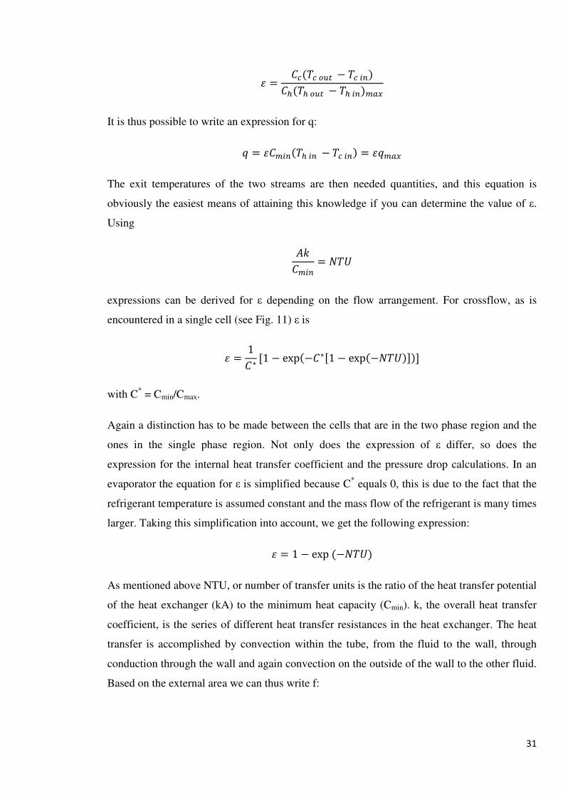
Heat exchangers can be analyzed using the ε-NTU method. This method only requires the inlet conditions of both fluids to calculate the heat transfer. The maximum possible heat transfer

���� � ����� �� � ��� (1)

is multiplied by the heat exchanger effectiveness in order to obtain the actual heat transfer. The effectiveness, ε, is determined by the geometry and the physical properties of the fluids. These properties are initially only known at the inlet conditions, iterations are therefore necessary so that the properties can be re-evaluated at average conditions.

By dividing the heat exchanger into smaller elements and solving them as separate heat exchangers, a more accurate simulation can be achieved because the variation in the properties can be taken into account. If these divisions are

D. Smith, student in the second year of Master of Electromechanical Engineering at Ghent University (UGent), Ghent, Belgium. E-mail: Dominic.Smith@UGent.be .

sections of tubes, two dimensional air distribution can be implemented, because every element can be assigned different air inlet conditions. For these reasons, this local analysis method is preferred to the lumped parameter scheme.

B. Fluid Properties

In evaporators both single as two phase flow are present. For both flow regimes different equations have to be implemented for the determination of the heat transfer coefficient, hint, and the pressure drop, ∆p. These parameters are needed to determine the effectiveness.

In two phase flow these factors show a great dependency on vapour quality which is the ratio of vapour mass flow to the total mass flow.

Table 1 shows the different applied correlations, they were chosen for accuracy and validity ranges.

Table 1 Applied Correlations

Air side heat transfer coefficient Chang and Wang [1] Single phase ref. heat transfer coefficient Wielandt Two phase ref. heat transfer coefficient Gungor and Winterton [2] Single phase pressured drop Blasius Two phase pressure drop Friedel [3] Grönnerud [4]

C. Computation path

As the outlet conditions from one element are used as the inlet conditions for the next element on the refrigerant path, it is important to keep track of the computation sequence of the tubes and elements. This is complicated by the fact that the refrigerant does not necessarily flow through consecutive tubes, it can for example go from the first tube of the first row to the third tube of the second row.

The refrigerant states are stored in a three dimensional matrix, where a row coincides with a tube. After solving an element the outlet conditions are then saved in the matrix at the position of the next element. An algorithm was developed to determine the sequence of tubes and elements.

D. Tube splitting

During evaporation more vapour becomes present in the tubes, resulting in higher velocities, due to the larger specific volume of vapour, and thus in a greater and often unacceptable pressure drop. In order to compensate this effect, tube splitting is encountered, thus decreasing the mass flow in every tube. At a tube split, the refrigerant distributes itself in appropriate proportions so refrigerant pressure drop in all branches from inlet to outlet is the same.

The pressure drop can be written as in (2).

∆� � ���

with S the flow resistance. The flow apportionment is determined using the flow resistance and the pressure drop. The mass flow rate will be greater in the circuits or branches of which the flow resistance is smaller. As these values are initially unknown, iterations are necessary.

III. MODEL VALIDATION

A. Water-air cases

In order to confirm the validity of the single phase heat transfer and pressure drop, air maldistribution, the flow apportionment as well as the software used to determine the fluid properties, test were run for water flowing in the tubes and air over the tubes, where water is the hot fluid and air the cold. These are not normal conditions for evaporators, but are used solely to validate the different components of the program.

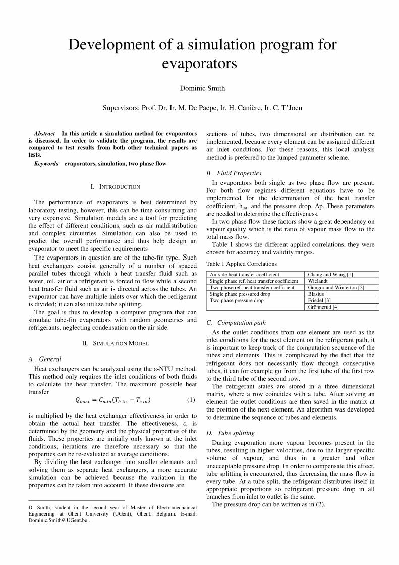
In figure 1 the simulation results are compared to the test results.

Figure 1Simulation results vs. test results

The simulations under predicted the heat transfer both for uniform as for non-uniform air distribution. The relative difference of the values was never more than 5%.

B. Evaporators

For validation of the model for evaporators with two phase flow, test cases can be found in literature. Kwon [5] provides enough parameters to run accurate simulations.

A discrepancy of -18.55% was found with Kwon’s data.This difference is unacceptable. As the simulation program works properly for the water-air heat exchanger, the cause of this discrepancy must be found in the properties specific toevaporators. The main differences are the presence of two phase flow and, in humid conditions, condensation on the tubes and fins on the airside. However, the two phase correlations have been tried and tested by the authors [2], suggesting that the lack of condensation in the model is the cause of the relative difference between the simulated data and the test data.

C. Condensation

As the water vapour present in the air comes into contact with a surface (fins and/or tubes) that is beneath the dew point temperature for water at that pressure, water is deposited on the surface and the latent heat is transferred to the refrigerant.

0

5000

10000

15000

20000

0 5000 10000 15000

Qsi

m [

W]

Qtest [W]

Without XProps

With XProps

(2)

with S the flow resistance. The flow apportionment is determined using the flow resistance and the pressure drop. The mass flow rate will be greater in the circuits or branches

low resistance is smaller. As these values are

ALIDATION

In order to confirm the validity of the single phase heat distribution, the flow

as well as the software used to determine the fluid properties, test were run for water flowing in the tubes and air over the tubes, where water is the hot fluid and air the cold. These are not normal conditions for evaporators, but are

date the different components of the

In figure 1 the simulation results are compared to the test

The simulations under predicted the heat transfer both for uniform air distribution. The relative

difference of the values was never more than 5%.

For validation of the model for evaporators with two phase flow, test cases can be found in literature. Kwon [5] provides

accurate simulations. 18.55% was found with Kwon’s data.

This difference is unacceptable. As the simulation program air heat exchanger, the cause of

this discrepancy must be found in the properties specific to evaporators. The main differences are the presence of two phase flow and, in humid conditions, condensation on the tubes and fins on the airside. However, the two phase correlations have been tried and tested by the authors [2],

f condensation in the model is the cause of the relative difference between the simulated data

As the water vapour present in the air comes into contact with a surface (fins and/or tubes) that is beneath the dew point

ature for water at that pressure, water is deposited on the surface and the latent heat is transferred to the refrigerant.

Calculations based on the psychrometric chart reveal that this heat transfer can be up to 50% of the sensible heat transfer.

D. Further Evaporator Cases

As condensation is not present in the model, it has to be validated in either dry conditions or with the sensible heat transfer in wet conditions. Domanski [6] provides such information. Two separate cases, with different circuit geometries were studied in detail. The overall heat transfer compared to the simulated values and the relative differences are given in table 2.

Table 2: Simulation results

QDom (W) Case 1 6590 Case 2 6680

The results show a good agreement with the values obtained from Domanski.

IV. CONCLUSION

A computer model was developed that successfully simulated evaporators with complex geometries, tube splitting and air maldistribution. The resultsthose of the equivalent test cases

The model does not include condensation of water vapour on the air side, which is a shortcoming as the program therefore does not predict the performance of an evaporator in normal operating conditions correctly. It does however provide good base for further development. Some features for condensation have already been implemented.

ACKNOWLEDGEMENTS

The author would like to thank the supervisors for providing the necessary help to complete this project.

REFERENCES

[1] C.C. Wang, C.J. Lee, C.T. Chang and S.P. Lin, friction correlation for compact louvered fin and tube heat exchangers

Int. J. Heat and Mass Transfer 42 (1999) pp. 1945[2] K.E. Gungor and R.H.S. Winterton,

Boiling in Tubes and Annuli, Int. J. Heat Mass Transfer 29 (1986) pp. 351-358

[3] L. Friedel, Improved friction drop correlations for horizontal and

vertical two-phase pipe flow

Meeting (1979) [4] R. Gronnerud, Investigation of liquid hold

transfer in circulation type of evaporators

l’Inst. du Froid (1979) [5] J. Lee, Y.C. Kwon and M.H. Kim

a fin and tube evaporator containing a zeotropic mixture refrigerant

with air maldistribution, Int. J. of Refrigeration 26 (2003) pp. 707[6] J. Lee and P.A. Domanski,

maldistributions on the performance of finned

R-22 and R-407C (1997)

15000 20000

Without XProps

With XProps

Calculations based on the psychrometric chart reveal that this heat transfer can be up to 50% of the sensible heat

Evaporator Cases

As condensation is not present in the model, it has to be validated in either dry conditions or with the sensible heat transfer in wet conditions. Domanski [6] provides such information. Two separate cases, with different circuit

s were studied in detail. The overall heat transfer compared to the simulated values and the relative differences

Qsim(W) RD (%) 6817 3.44 6912 3.47

The results show a good agreement with the values obtained

ONCLUSION

A computer model was developed that successfully simulated evaporators with complex geometries, tube splitting

. The results are always within 5% of those of the equivalent test cases, which is acceptable.

The model does not include condensation of water vapour on the air side, which is a shortcoming as the program therefore does not predict the performance of an evaporator in normal operating conditions correctly. It does however

good base for further development. Some features for condensation have already been implemented.

CKNOWLEDGEMENTS

The author would like to thank the supervisors for providing help to complete this project.

EFERENCES C.C. Wang, C.J. Lee, C.T. Chang and S.P. Lin, Heat transfer and

friction correlation for compact louvered fin and tube heat exchangers, Int. J. Heat and Mass Transfer 42 (1999) pp. 1945-1956

R.H.S. Winterton, A general correlation for Flow-

, Int. J. Heat Mass Transfer 29 (1986) pp.

Improved friction drop correlations for horizontal and

phase pipe flow, European Two-phase Flow Group

Investigation of liquid hold-up, flow-resistance and heat

transfer in circulation type of evaporators. In Annexe 1972-1, Bull. de

M.H. Kim, An improved method for analyzing

a fin and tube evaporator containing a zeotropic mixture refrigerant

Int. J. of Refrigeration 26 (2003) pp. 707–720 J. Lee and P.A. Domanski, Impact of air and refrigerant

s on the performance of finned-tube evaporators with

CONTENTS

Nomenclature 1

1 Introduction 3

1.1. Problem description

1.2. Goal of thesis

References

2 Literature Survey 5

2.1. Overview of literature survey

2.2. Calculation methods at tube level

2.2.1. Lumped analysis scheme

2.2.2. Local analysis schemes

2.2.3. Calculation Methods

2.3. Calculation at heat exchanger level

2.3.1. The general idea

2.3.2. Variations

2.3.3. Flow apportionment

2.4. Comparison

References

3 General Concepts 17

3.1. Two-phase flow

3.2. Tube-fin heat exchanger

3.3 Computer Program

References

4 Computation Sequence 22

4.1. Computational path

4.2. Air and Refrigerant States

References

5 Cell Calculations 30

5.1. Single phase cell

5.2. Two phase cell

References

6 Flow and Heat Exchanger Properties 40

6.1. External Heat Transfer Coefficient

6.2. Internal heat transfer coefficient

6.3. Fin efficiency

References

7 The Refrigerant Pressure drop 54

7.1. Single Phase Flow

7.2. Two Phase Flow

References

8 Heat Exchanger calculations 59

8.1. Tube calculations

8.2. Heat exchanger simulation

8.3. Flow apportionment

References

9 Model validation 69

9.1. Water-air

9.1.1. Uniform air distribution

9.1.2. Non-uniform air distribution

9.2. Pressure correction

9.3. Evaporator

9.4. Condensation

9.5. Further Evaporator Cases

References

10 Conclusion 96

Appendix A 97

1

NOMENCLATURE

Symbol Discription Units A Area m² cp Specific heat capacity J/kg.K C Heat capacity kW/K Do Outer tube diameter m Di Inner tube diameter m Dc Fin collar outside diameter m Dh Hydraulic diameter m dp Pressure drop bar f Fanning factor - Fp Fin pitch m Fh Fin height m Fr Froude number - g Acceleration due to gravity m/s² G Mass velocity g/m²s hLG Enthalpy of evaporation kJ/kg hi Internal heat transfer coefficient W/m²K ho External heat transfer coefficient W/m²K htp Two phase heat transfer coefficient W/m²K j Colburn factor - k, U Overall heat transfer coefficient W/m²K L Segment length m Lp Louver pitch m Lh Louver height m m Mass flow rate kg/s M Molecular weight kg/kg mol Nu Nusselt number - NTU Number of transfer units - p Pressure bar pr Reduced pressure bar Pl Longitudinal spacing (Xl) m Pt Transversal spacing (Xt) m Pr Prandtl number - Q, q Heat transfer rate W r radius m Re Reynolds number - T Temperature °C Tw Wall Temperature °C v Velocity m/s x vapour quality - δ Distribution - δf Fin thickness m ε Heat exchanger effectiveness - � Void fraction - ηf Fin efficiency - λ Thermal conductivity W/mK λw Thermal conductivity tube wall W/mK

2

µ Dynamic viscosity Pa.s ρ Density kg/m³ σ Surface tension N/m ω Humidity Ratio kg water/kg air Subscripts

a air i internal r refrigerant o exertnal g gas w wall l liquid w water c cold t tube h hot c circuit min minimum b branch max maximum f fin

Abreviations

HTC Heat Transfer Coefficient HEX Heat Exchanger

3

Chapter 1

Introduction

1.1. Problem description

Air-to-refrigerant heat exchangers (HEX), such as plate-fin-tube coils (evaporators), form an

important part of air conditioning and refrigeration systems. They play a major role in the

energy consumption and manufacturing costs of the entire system. The traditional design

methods such as the analytical or graphical approach are often ineffective due to the

complexity of modern heat exchangers. The complexity includes geometry, circuitry, non-

uniform airflow, the effects of multi-phase flow and the use of various types of refrigerants. A

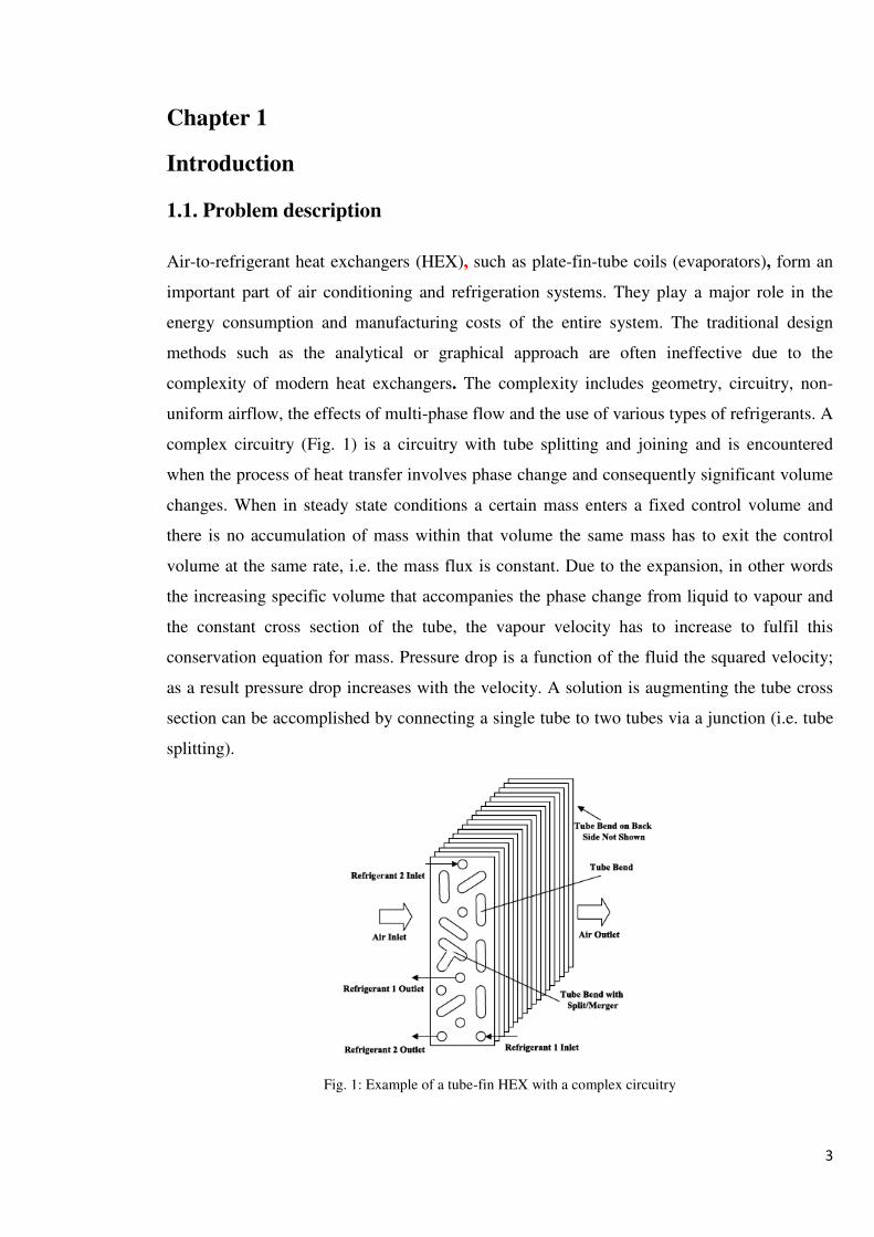
complex circuitry (Fig. 1) is a circuitry with tube splitting and joining and is encountered

when the process of heat transfer involves phase change and consequently significant volume

changes. When in steady state conditions a certain mass enters a fixed control volume and

there is no accumulation of mass within that volume the same mass has to exit the control

volume at the same rate, i.e. the mass flux is constant. Due to the expansion, in other words

the increasing specific volume that accompanies the phase change from liquid to vapour and

the constant cross section of the tube, the vapour velocity has to increase to fulfil this

conservation equation for mass. Pressure drop is a function of the fluid the squared velocity;

as a result pressure drop increases with the velocity. A solution is augmenting the tube cross

section can be accomplished by connecting a single tube to two tubes via a junction (i.e. tube

splitting).

Fig. 1: Example of a tube-fin HEX with a complex circuitry

4

1.2. Goal of thesis

The goal of this master thesis is to develop a simulation program for plate-fin-tube

evaporators starting from the simulation code created by F. Vanhee and C. T’Joen which was

written for single phase fluids in the tubes and for a fixed circuitry (specified in the software).

To obtain a more general program the following algorithms have to be added:

• An algorithm which traces the refrigerant through a complex circuitry that includes

tube splitting and joining. This algorithm has to ensure that the pressure drops over

two parallel branches are balanced by adjusting the mass flux at the entrance of the

branches. Secondly, it should determine appropriate mixing expressions at junctions,

in other words the refrigerant properties at the entrance of two parallel branches

should be derived from the single tube upstream of the junction. Finally, it should

determine a calculation path in an intelligent manner.

• A routine to determine the heat transfer coefficients for two phase flow in the tubes.

5

Chapter 2

Literature Survey

2.1. Overview of literature survey

Different numerical models for the evaluation of heat exchangers exist; the goal of this study

is to compare these models and to come to a conclusion concerning the most efficient solution

in terms of computing time and accuracy. The make-up of the following passage is as follows:

first an overview of the different calculation methods at tube level is given, then a summary of

algorithms used to track the complex circuitry and finally a general comparison between the

different methods.

2.2. Calculation methods at tube level

2.2.1. Lumped analysis scheme

The analysis of a heat exchanger can be approached in two distinct manners. The first

approach is a lumped analysis scheme. The heat exchanger is considered as a single unit, with

an in- and outlet for air and an in- and outlet for refrigerant. A mean temperature or air

enthalpy difference is found for the entire coil which is then used to calculate the total heat

transfer; a constant heat transfer coefficient (HTC) is assumed for the entire coil. This method

has been described in ASHRAE [1].

2.2.2. Local analysis schemes

The second approach is a local analysis scheme; the heat exchanger is divided into multiple

segments. Every segment is calculated as a separate unit and the outlet from one unit is used

as the inlet for the adjacent segment. By doing this a non-uniform air-distribution can be

implemented, because every segment (also called node or element) can be given its own air

inlet conditions, and changes in physical properties due to the phase change within the tubes

can be taken into account.

6

Fig. 2: Example of elementary segment

There are several possibilities for the choice of the elementary unit. A first option, used by

Ellison et al. [2] and Domanski [3], uses a tube as the local analysis unit, consequently only

allowing the modelling of one-dimensional air flow distribution because the air flow along the

tube is assumed constant.

Fischer et al. [4] suggest dividing the heat exchanger in three regions: the two-phase region,

the transition region and the superheated region. The variation of HTC along the pipe in the

two-phase region can be determined by assuming the refrigerant quality varies proportional to

the pipe length. Studies show that major changes in HTC occur between a refrigerant quality

of 0.0 (saturated liquid) to 0.4. Above a quality of 0.4, there is very little change of HTC. It is

therefore reasonable to further divide the two-phase region into two control volumes (Fig. 3).

This technique permits the use of different HTC dependent of the region, but does not give the

possibility to simulate a comprehensive air maldistribution.

Fig. 3: Heat exchanger divided in four regions

7

A third model discretizes the coil along the coolant path, the coil is thus divided into a three-

dimensional array (Fig. 4) of heat exchangers (Fig. 2), each of which is formed around a

portion of coolant tube; this method is used by Vardhan [5], Judge [6], Ge [7], Lee [8] and

Jiang [9] among others. The elements can either be of a constant length (Fig. 2) or can have a

length depending on the properties of the flow at that point (Fig. 5), for example it would be

desirable to use smaller elements in regions where there is a great variation in HTC and larger

segments where the HTC is almost constant. Implementing a three dimensional non-uniform

air distribution is now possible.

Fig. 4: 3D array of elementary constant size HEX forming a complete HEX

Fig. 5: Example of possible subdivisions

Chwalowski et al. [10] predicted the performance of evaporators using four different methods,

and compared their results with test data. They showed that simulated or imposed air velocity

profiles must follow the actual air distribution across the coil for successful capacity

prediction of a coil. In their laboratory tests, the capacity degradation was up to 30% for mal-

8

distributed air velocity profiles. Due to the large discrepancies when not using an air velocity

profile close to reality the use of lumped analysis or local analysis schemes which do not

allow a full implementation of air maldistribution is not advised.

2.2.3. Calculation Methods

To simplify the calculations several assumption are made which do not alter the outcome in a

significant way, they are:

• the heat exchanger operates under steady state conditions (i.e., constant flow rate and

fluid temperatures at the inlet and within the exchanger are independent of time)

• heat losses to the surroundings are negligible

• the individual and overall heat transfer coefficients are constant throughout the

exchanger

• longitudinal conduction in the fluid and wall is negligible

• the overall surface efficiency is uniform and constant

Iterative method

The calculation methods can be placed in two categories: iterative methods and the matrix

formalism method. The iterative method used by Vardhan, Lee and Jiang can be described as

follows: In the first step the air inlet conditions of every segment are assumed the same as the

inlet conditions of the HEX. The calculations start at the first element on the coolant path of

which the refrigerant inlet conditions are known and the air inlet conditions are assumed,

making it possible to calculate the heat transfer (and refrigerant pressure drop) using for

example the ε-NTU method. The outlet conditions of the refrigerant and the air for this

segment are thus found, these conditions can be used as inlet conditions respectively for the

next element on the coolant path and for the element behind (with respect to the airflow) this

segment. In this manner all segments are calculated following the refrigerant path until the

end is reached. In the second step the inlet conditions are updated using the data retrieved

from the first iteration and another march along the coolant path is made. This sequence can

be repeated until the difference in conditions between two consecutive marches is small, how

small the difference has to be can be specified.

9

Fig. 6: Elements (nodes) along coolant path

For completeness, a less common approach is mentioned which, as proposed by Mirth et al.

[11], discretizes the coil along the air path. The outlet temperature of the refrigerant is

assumed and a stepwise march is conducted along the air path until the refrigerant inlet

temperature matches the actual inlet temperature.

Matrix formalism

The matrix formalism method can be described as follows: in- and outlet temperatures, i.e. the

temperatures of the fluid streams entering and exiting a heat exchanger segments, are related

to each other by the energy balance of that segment. For every element four equations can be

written: the heat entering the element with the refrigerant, the heat leaving with the refrigerant

which is the equal to the heat entering plus the heat transferred from the air, the heat entering

with the air and finally the heat leaving with the air which is the heat entering minus the heat

transferred to the refrigerant.

�� � ����,��

�� � ����,�� ����,� ��,��� ��� � ����,���

��� � ����,��� �����,�� �,�� With U the overall heat transfer coefficient and A the surface area of the tubes, these are

assumed constant within every element and the hot and cold temperatures are assumed to vary

10

linearly along the flow. T1 the refrigerant inlet temperature, T11 the air inlet temperature, T2

the refrigerant outlet temperature and T12 the air outlet temperature, with �,� � 0,5� " �� and ��,�� � 0,5�� " ���. These equations can be rewritten in matrix form:

����,� 0 0 0 T1 ��

����,� ��/2 ��/2 ��/2 ��/2 T2 ��

0 0 ����,� 0 T11 ���

��/2 ��/2 ����,� ��/2 ��/2 T12 ���

Assembly of the element characteristics for all elements results in a global stiffness matrix.

The equations for the entire heat exchanger are solved simultaneously by matrix inversion.

This analysis may not give accurate results due to the simplifying assumptions made;

generalizing this method to complex situations is difficult. This method is however in closed

form, which means the amount of calculations is fixed and can be solved in finite time.

2.3. Calculation at heat exchanger level

As a result of the friction loss due to the high vapour velocity, splitting and combination of

the refrigerant flow is necessary to offer an acceptable pressure drop in the tubes. The

complex geometry can also provide a more uniform temperature distribution and thus a better

performance.

=

11

Fig. 7: Tube splitting and joining

Important in tube splitting and joining is that the apportionment of refrigerant flow at a split is

such that the downstream pressure drops of the two branches are balanced. Furthermore,

appropriate mixing expressions at junctions should be obtained (Fig. 7), in other words the

refrigerant properties at the entrance of two parallel branches (branch 11 and 22 in Fig. 7b)

should be derived from the single tube upstream of the junction (branch 1 in Fig. 7b) and the

properties at the inlet of single tube (branch 12 in Fig. 7a) are derived from those of the two

tubes upstream of the preceding junction (branch 1 and 2 in Fig. 7a).

2.3.1. The general idea

In order to simulate a coil with complex circuitry, a special approach is proposed by Liang et

al. [12] to link all the control volumes in computation. The method suggested by Ellison et al.

[2] differs through the fact that Liang’s approach can readily be used to simulate a coil based

on control volumes. The method of Liang is quoted here: A simplified branch network

diagram is required first to trace the joining and branching of refrigerant flow. Although the

refrigerant circuitry may be complex, the branch network is usually quite simple. In this way,

the whole coil can be regarded as a network consisting of several separated branches. … To

simulate a coil, a hierarchical system is used, which follows the procedure given below:

a. First level: to determine the computation sequence for all branches in the coil and

carry out computation branch-by-branch.

b. Second level: to determine the computation sequence for all tubes in the branch and

carry out computation tube-by-tube.

7a 7b

12

c. Third level: to determine the computation sequence for all control volumes in the tube

and carry out computation control volume-by-control volume.

The main problem in the first level is to specify the iteration sequence for all the branches. In

order to develop a general program that can simulate the coils with all kinds of refrigerant

branch networks, a two-direction adjacent matrix of the graphic theory is used to describe the

connection of refrigerant branches. … In the second level, two arrays are introduced for each

branch to indicate the address of each tube in the coil. … In the third level, the computation

sequence of control volumes in each tube is also along the refrigerant direction.

2.3.2. Variations

Other approaches follow essentially the same three level pattern, they mainly differ within a

level. As mentioned above Ellison uses a tube by tube approach, the third level is therefore

redundant. Here, the tubes have two position indices I and J; I denotes the position of the tube

within a row, J numbers the row. Elements of four 3-dimensional arrays are associated with

each tube so that the indices of tubes that feed or receive refrigerant to or from tube I, J can be

stored. The arrays INI(I,J,K) and INJ(I,J,K), K = 1 or 2, will contain indices of tubes that

supply refrigerant to tube I,J; OUTI(I,J,K) and OUTJ(I,J,K) contain the addresses of tubes

that receive the outflows. Kuo et al. [13] describe a complete algorithm; to trace the

refrigerant flow they use an array with indices of n, i, j and m. The meaning of the indices are

as stated below:

n: denotes the number of main flows before entering the heat exchangers.

i: refers to as the number of the first level circuitry, and the associated values can

be 0, 1, or 2. For example, the value of 0 indicates that it is at the position

without splitting or is at the location where circuitry are combining at the end.

The value of 1 indicates this part is inherited from the first level. Notice that

the value can be easily extended to higher values (>2), for splitting from or re-

combining to more than two tubes. The algorithm by Ellision et al. [2] is

strictly limited to two tubes.

j: refers to as the number of the second level circuitry, and the associated values

can be 0, 1, or 2. For example, the value of 0 indicates that it is at the position

without splitting or is at the location where circuitry is combining at the end.

The value of 1 indicates this part is inherited from the first level. Notice that

13

the value can be easily extended to higher value (>2) if splitting from or re-

combining to for more than two tubes.

m: denotes as the splitting/combining index, the corresponding value is from 0 to

6.

Relevant meaning is as follows:

0: normal node in the circuitry.

1: inlet of the heat exchanger.

2: splitting node.

3: after splitting.

4: before combining.

5: combining node.

6: outlet of the heat exchanger.

Jiang et al. [9] proposed a similar technique in their simulation tool CoilDesigner. A junction-

tube connectivity matrix is defined to describe the location relationship between junctions and

tubes. The relationships are as follows:

JTA[j,i]=1: junction j is upstream and connected to tube i

JTA[j,i]=-1: junction j is downstream and connected to tube i

JTA[j,i]=0: junction j is not connected to tube i

The junction-tube connectivity matrix makes it possible to track the refrigerant flow from

inlets to outlets so the energy balance relationship can be established between the upward

stream and downward stream; it also describes the direction of the flow, 1 denoting from left

to right and -1 from right to left. Based on the tube location irow (number of row) and iver

(vertical positon of tube) and the refrigerant flow direction idir of the tube, the predecessor and

the successor segments of the neighbouring tubes can be identified, for the purpose of energy

and mass conservation analysis on the airside.

2.3.3. Flow apportionment

To obtain the correct refrigerant apportionment at a split, in the first iteration an even

distribution is assumed and the pressure drop is calculated accordingly. If at the next branch

joining the pressure drops of the two branches are not balanced, the mass flow is adjusted at

the previous split and the pressure drop is recalculated in a second iteration and so on. When

14

the branches are balanced, the inlet conditions for the segment after the rejoining are weighted

average values of the separate joining branches.

2.4. Comparison

The simplifying assumptions have an effect on the accuracy of the simulation model:

• Neglecting the longitudinal conduction through the pipes, fins and fluid however

does not influence the performance in most HEX, it only becomes an important factor

in HEX where great temperature gradients are encountered, such as in cryogenic

systems.

• The assumption concerning the constant HTC is avoided by the use of sufficiently

small elements in the local analysis scheme.

• A HEX generally runs in steady-state conditions, therefore only considering steady-

state is acceptable to rate the performance.

• Finally, the assumption that the overall surface efficiency is constant has to be viewed

in historical context; it has grown from the study of cylindrical fins and has been

adopted in later models although the geometries have become more complex. It has

been generally accepted as no other alternatives are available

The different approaches have advantages and disadvantages, thus making the choice less

than straightforward. At the tube level, it is apparent that the local scheme analysis has a

greater accuracy than the lumped scheme: Since the divided segments can be made small

enough, the formulae for the calculation of local HTC and pressure drop for fluids in the HEX

can be utilised directly and thus a higher degree of accuracy can be expected. This method can

also be used to simulate heat exchangers with complicated circuits and pipe arrangements and

is suitable for the calculation of optimal design for single heat exchangers. The critical

shortcoming of this method is the computing time, compared with the lumped analysis

scheme the computing time is about ten times longer. However, a comprehensive air mal-

distribution can be implemented of which the importance was demonstrated by Chwalowski

et al. [10].

Using the iterative method to calculate the heat transfer and pressure drop can potentially

have fewer computations than the matrix formalism. After determination of the HTC and

other parameters to calculate the heat transfer and pressure drop this method only needs one

15

calculation per element per iteration plus the process of storing the outlet conditions (air and

refrigerant). It is however not a closed form method, a solution can thus not be guaranteed

within a reasonable time because the amount of iterations to reach convergence is not known

from the start. Using the matrix formalism a closed form expression can be obtained for the

heat exchanger, but the computations include inverting a sizeable matrix, which requires

additional software. When considering just one element, we see that the resulting matrix is

4x4, thus needing not only 16 computations to invert it, but also needing storage of the matrix

and its inverse and matrix multiplication, which consists of another 4 computations, to

achieve a result. In the same amount of calculations 7 iterations can be achieved, which will

more often than not be sufficient. The iterative method thus generally requires fewer

calculations and offers the possibility to define the accuracy by adjusting the tolerance for

convergence, for that reason it is commonly accepted.

The proposed refrigerant tracing methods are very similar. Ellison’s method can be excluded

from this discussion due to discarded tube-by-tube method. The scheme proposed by Kuo et

al. [13] is limited to two consecutive splits but can easily be extended, this requires an

additional index in the array. The proposals of Jiang [9] and Liang [12] only differ in the

manner of storing the tube connections; Jiang’s method however is slightly more intuitive and

is therefore preferred.

16

REFERENCES

[1] ASHRAE Handbook, American Society for Heating, Refrigeration and Air-

Conditioning Engineers, Inc. Vol. Equipment Volume. 1983.

[2] Ellison, R., et al., A computer model for air-cooled refrigerant condensers with

specified refrigerant circuiting. ASHRAE transactions, 1981: p. 1106-1124.

[3] Domanski, P.A., Simulation of an evaporator with non-uniform one-dimensional air

distribution. ASHRAE Trans 97, 1991: p. 793-802.

[4] Fischer, S.K., The Oak Ridge heat pump models: a steady-state computer design

model for air-to-air heat pumps. Oak Ridge TN: The Oak Ridge National Laboratory, 1983.

[5] Vardhan, A. and P.L. Dhar, A new procedure for performance prediction of air

conditioning coils. International Journal of Refrigeration-Revue Internationale Du Froid, 1998. 21(1): p. 77-83.

[6] Judge, J. and R. Radermacher, A heat exchanger model for mixtures and pure

refrigerant cycle simulations. International Journal of Refrigeration-Revue Internationale Du Froid, 1997. 20(4): p. 244-255.

[7] Ge, Y.T. and R. Cropper, Air-cooled condensers in retail systems using R22 and

R404A refrigerants. Applied Energy, 2004. 78(1): p. 95-110.

[8] Lee, J.H., et al., Experimental and numerical research on condenser performance for

R-22 and R-407C refrigerants. International Journal of Refrigeration-Revue Internationale Du Froid, 2002. 25(3): p. 372-382.

[9] Jiang, H.B., V. Aute, and R. Radermacher, CoilDesigner: a general-purpose

simulation and design tool for air-to-refrigerant heat exchangers. International Journal of Refrigeration-Revue Internationale Du Froid, 2006. 29(4): p. 601-610.

[10] Chwalowski, M., Verification of evaporator mcomputer models and analysis of

performance of an evaporator coil. ASHRAE Trans 89, 1989.

[11] Mirth, D.R., Prediction of cooling coil performance under condensing conditions. Int. J. Heat and Fluid Flow, 1993.

[12] Liang, S.Y., T.N. Wong, and G.K. Nathan, Numerical and experimental studies of

refrigerant circuitry of evaporator coils. International Journal of Refrigeration-Revue Internationale Du Froid, 2001. 24(8): p. 823-833.

[13] Kuo, M.C., et al., An algorithm for simulation of the performance of air-cooled heat

exchanger applications subject to the influence of complex circuitry. Applied Thermal Engineering, 2006. 26(1): p. 1-9.

17

Chapter 3

General Concepts

3.1. Two-phase flow

In evaporators the refrigerant boils in the tubes and cools the fluid that passes over the

outsides of the tubes. The refrigerant passing through the evaporator undergoes a phase

change; the fluid entering the evaporator becomes vapour along the coolant path. This is not

an instantaneous process, but takes time and space. The transition between both single phase

regions is called the two-phase region, in this region fluid and vapour coexist. The refrigerant

shows different flow patterns depending on the ratio of vapour present, the velocity, surface

tension and gravity; horizontal pipes will show different flow regimes to vertical. The pattern

has influence on the heat transfer and pressure drop in the tubes in which the refrigerant

flows.

The two-phase region is represented in the P-h diagram by the area under the dome. The

refrigerant entering the evaporator usually already consists of both phases, the coolant exiting

should be purely vapour in order not to damage the compressor that follows the evaporator in

the thermodynamic cycle. The operating field for evaporators working with R22 is shown in

Fig. 8.

18

Fig. 8: P-h Diagram of R22

In the two phase region, thus during evaporation, temperature is fixed for a given pressure.

This means that a temperature and pressure are not sufficient to define the state of the

refrigerant within this region, as is possible in the single phase region. However, temperature

or pressure and vapour quality are. Vapour quality is defined as the ratio of mass of the gas to

the total mass:

% � �&'�&' " �(' With these two parameters a well determined point in the P-h diagram is defined.

In horizontal pipes four flow regimes can be distinguished depending on the quantity of

vapour present. They are:

a) Dispersed bubble flow: the gas bubbles flow mainly towards the top of the pipe

b) Slug flow: the gas bubbles join and from bigger gas regions that are followed by liquid

areas

c) Stratified wavy flow: the amplitude of the waves increases as the vapour velocity

increases. Liquid droplets are swept along in the gas phase.

d) Annular dispersed flow: the liquid film on the bottom is thinner than at the top due to

gravity.

3.2. Tube-fin heat exchanger

Tube and fin heat exchangers are widely used in a variety of applications in the fields of

refrigeration, air conditioning and the like. Such heat exchangers

number of spaced parallel tubes through which a heat transfer fluid such as water, oil, air or a

refrigerant is forced to flow while a second heat transfer fluid such as air is directed across the

tubes. To improve heat transfer a plurality of fins comprising

placed on the tubes.

generally at right angles to the fin, and a large number of the fins are arranged in parallel,

closely spaced relationship along the tubes

exchange fluid to flow across the fins and around the tubes. The tubes and plates are provided

with a suitable mechanical and thermal bond, for example by expansion of the tubes after

assembly of the fin pl

Annular dispersed flow: the liquid film on the bottom is thinner than at the top due to

Fig. 9: Flow Patterns is Horizontal Pipes

fin heat exchanger

exchangers are widely used in a variety of applications in the fields of

refrigeration, air conditioning and the like. Such heat exchangers

of spaced parallel tubes through which a heat transfer fluid such as water, oil, air or a

refrigerant is forced to flow while a second heat transfer fluid such as air is directed across the

tubes. To improve heat transfer a plurality of fins comprising

placed on the tubes. Each fin plate has a number of openings through which the tubes pass

generally at right angles to the fin, and a large number of the fins are arranged in parallel,

closely spaced relationship along the tubes to form multiple paths for the air or other heat

exchange fluid to flow across the fins and around the tubes. The tubes and plates are provided

with a suitable mechanical and thermal bond, for example by expansion of the tubes after

assembly of the fin plates, to provide good thermal conduction.

19

Annular dispersed flow: the liquid film on the bottom is thinner than at the top due to

exchangers are widely used in a variety of applications in the fields of

refrigeration, air conditioning and the like. Such heat exchangers consist generally of a

of spaced parallel tubes through which a heat transfer fluid such as water, oil, air or a

refrigerant is forced to flow while a second heat transfer fluid such as air is directed across the

tubes. To improve heat transfer a plurality of fins comprising thin sheet metal plates are

through which the tubes pass

generally at right angles to the fin, and a large number of the fins are arranged in parallel,

to form multiple paths for the air or other heat

exchange fluid to flow across the fins and around the tubes. The tubes and plates are provided

with a suitable mechanical and thermal bond, for example by expansion of the tubes after

20

Fig. 10: Tube-Fin Heat Exchanger

The performance of the heat exchanger can be determined by either tests or simulations. The

advantages of simulations are extensive. Simulations do not require prototypes which cost

time and money, parameters can simply be altered without the need to build a new model and

test stands are unnecessary. On the other hand, simulation models have to be verified, many

different test cases are needed to confirm the validity of the model. However, once confirmed,

a computer model will soon save both time and money. Simulation programs are thus

valuable tools for the design en development of evaporators.

As mentioned in the literature survey, there are different models available to create a program.

The model of choice is the local analysis scheme. Here the heat exchanger is divided into

smaller elements or cells that are easily calculable. A cell consists of a part of a tube and the

fins surrounding this part. The advantages of these subdivisions are that the variation of

physical properties can be taken into account and a non-uniform air distribution can be

implemented. Within every cell the properties are considered constant and the average of the

in- and outlet states. Each cell can be solved because the inlet conditions on both the airside

and the refrigerant side are known.

Fig. 11: A Single Cell

21

Fig. 12: Side View of Heat Exchanger Dived into cells

3.3 Computer Program

For the design of a computer program that can run on standard desktop computers, C++ was

chosen as programming language. C++ is a straightforward choice due to its availability and

intuitiveness of the language. Input such as heat exchanger layout is entered via text files,

which the program interprets. Other information like tube geometry entered directly into the

program. However, the possibility to read all input from external files is present.

The physical properties of all fluids are firstly entered via tables in which values have to be

interpolated. Later an external program named XProps is used to calculate physical properties.

Afterwards results of both methods can be compared.

22

Chapter 4

Computation Sequence

4.1. Computational path

The cells in which the evaporator is divided have to be calculated in a certain sequence

because the inlet of a cell is the same as the outlet of the previous cell in the refrigerant path.

The configuration of the heat exchanger is not always straightforward; the tubes are not

necessarily connected to adjacent tubes. Furthermore, tube splitting is encountered.

The phase change from liquid to gas in the evaporator is accompanied by a change in specific

volume. A kilogram gas fills a bigger volume than a kilogram liquid. The mass flow rate in

the tubes is constant as there is no way for mass to escape. The following equation thus shows

that for a constant flow area the velocity has to increase because the density decreases:

�' � �. �. *

For example for R22 the density decreases at a saturation temperature of -10°C from

approximately 15.3 kg/m3 to 1.3 kg/m3, which is roughly 12 times smaller, meaning that the

velocity would increase 12 times. The correlation for pressure drop in the tubes however

includes the factor v2, consequently the pressure drop increase dramatically with increasing

velocity. Without any changes to the evaporator configuration the pressure drop will become

unacceptable.

The equation also shows that increasing the cross section is a possible solution. This can be

achieved by splitting a tube into two different tubes, thus doubling the total flow area and

reducing the vapour velocity. The resulting tubes can then be arranged to maximize the heat

transfer.

It is clear that an algorithm is necessary to correctly determine the computation sequence of

the cells, taking both tube splitting and tube arrangement into account.

Before the program can determine the computation sequence of the cells, the geometry of heat

exchanger has to be entered. As mentioned before, this is done by means of a text file (*.txt).

The contents of this file should unambiguously define the complex circuitry. Therefore the

23

method proposed by Liu et al. [1] is implemented. In this method a matrix, called a

connectivity matrix, is used. The dimension of the square matrix equals the number of tubes

in the evaporator plus two. The two extra rows/columns represent the inlet and outlet. A

simple example is given:

Fig. 13: The Evaporator Configuration

Fig. 14: The Connectivity Matrix

In the simple configuration shown in Fig. 13 the heat exchanger consists of 8 tubes, the matrix

is thus a 10x10 matrix, with row 0 representing the inlet and column 9 the outlet. The matrix

in Fig. 14 shows that the inlet is connected to tube 8 as a 1 is placed at the ninth (and not

eighth due to the inclusion of imaginary tube 0) position in row 0. Row 9, representing tube 8,

shows that tube 8 is connected to tube 4. Tube 4 (fifth row) is split into tube 3 and tube 7. And

so on. Finally, tube 1 is connected to the outlet.

24

Once the connectivity matrix is created and read into the program, the program must interpret

the matrix, this is done by an algorithm explained by the flow chart in Fig. 15. The example

given above was taken from the previously mentioned paper by Lui, in this case there is tube

joining. However, in evaporator used for domestic appliances there is no need for joining.

Although the implemented code to determine the computation sequence can take joining into

account, the flow chart gives a simplified algorithm for evaporators with only tube splitting.

Furthermore, tubes are only split into two tubes and there can only be one split per circuit.

25

Fig. 15 : Flowchart determination of Computation Path

tube = Out[0][e] Add tube to branch b

t = tube

yes

Temp empty no tube = temp

yes e<Out[0].size

t = tube

no

If Out[t].size > 1 (if there’s a split following tube t) Add tube=Out[t][0] to branch b+1and b = b+1

Add tube2=Out[t][1] to branch b+2 Store tube2 in temp

Else add tube=Out[t][0] to branch b

tube = exit (number of tubes +1)

Read row t of Connectivity Matrix If tube t supplies other tubes, store tube number in Out[t]

(element = 1 in matrix row)

t = number of tubes + 1

Read Connectivity Matrix Create vector of vectors “Out” to store the tubes

receiving refrigerant from the tube

t = 0 t = t+1

no

yes

Determine the number of branches by counting the number of splits + the number of entrances. When one branch splits into two,

there are three branches: the original plus the two new ones.

First entrance e = 0 and b = 0

e = e+1

Stop

26

An example of the input and output computational path are given in Fig. 16 and 17.

Fig. 16: Example Input

Fig. 17: Corresponding output

The position of the tubes in the evaporator is determined by the number given to the tube.

When reading in the connectivity matrix the program counts the number of tubes, which is the

dimension of the matrix minus two. The number of rows or screens is given as input to the

program. The numbers run from the top tube on the air inlet side to the bottom tube on the air

outlet side, the rows are passed through from top to bottom.

1 4 16 2 2 3 16 2 5 16 7 8 9 9 10 11 16 9 12 16 13 6 14 16 15

27

Fig. 18: Tube Numbering

Using the number of rows and the tube number the position is determined by the following

formulae:

+,- ./�01+ � 23,,+ 4+� 1�6 7

�,89:9,.8 -9:;9. +,- � � 23,,+ 4+� 1�6 7 < 6+ 1

With r the number of rows, N the total number of tubes and p the tube number. The

numbering of the positions starts at 0, for example tube 1 is in row 0 in position 0.

4.2. Air and Refrigerant States

To describe a system and predict its behaviour requires knowledge of its properties and how

those properties are related. The word ‘state’ refers to the condition of a system as described

by its properties. Since there are normally relations among the properties of a system, the state

often can be specified by providing the values of a subset of the properties.

A class ‘State’ is created in the program to store data of the states of the air and the

refrigerant. On the air side a state includes data such as temperature, pressure, velocity, mass

flow and absolute humidity. Although the condensation process on the airside is not taken

28

into account in this simulation model, some necessary steps have been implemented so that

the code can easily be expanded to take wet air into account.

The states of the refrigerant within the tube are a more difficult proposition. A clear

distinction has to be made between single phase states and two phase states. Again a state

consists of data such as temperature, pressure, velocity and mass flow, but also includes

vapour quality. In the single phase region pressure and temperature are not linked. During

evaporation however they are: with a certain pressure a certain temperature corresponds. A

state can thus be defined by mass flow, pressure and velocity or mass flow, temperature and

velocity.

As input for the computer program several states have to be given. A first state is the inlet

state of the refrigerant, more often than not the state is defined by the pressure, the quality and

the mass flow, the velocity can then be calculated using the geometry of the pipes and the

density at the given temperature. Secondly the states of the air have to be specified. Two

different options are available: all cells are set to the same state, this is called a uniform air-

distribution or a different state is defined for every cell of the first row of tube, in the case we

speak of a non-uniform air-distribution. Because the tubes are often staggered, which means

that the tubes of the second row aren’t behind the tubes of the first row, but are in between,

the inlet states of the second row are a combination of the outlet states of the previous screen

of tubes. For all but the top or the bottom tube of a screen the inlet states are the averages of

the outlets states of the two tubes directly in front of the tube in question. This means that the

velocity, temperature are weighted averages, while the mass flow is a simple average and the

pressure is unaffected. Fig. 12 shows such a staggered heat exchanger, we can see that the

bottom tube of the second row is not directly behind two tubes but only succeeds one tube,

averages are not used in this case, the conditions are the same as the preceding tube on the air

path, except that the mass flow is halved.

Before the actual calculations, the states are stored for every cell. Every cell has three states,

namely refrigerant inlet, air inlet and air outlet. The refrigerant outlet is equal to the inlet of

the next cell. Initially the states are all the same on the refrigerant side. For the airside the

inlet states and the outlet states of every row are set to the inlet conditions of the first row of

tubes.

29

Two 3 dimensional matrixes are created to keep track of the states. The first one stores the

refrigerant conditions with as dimensions the number of rows, the number of tubes per row

and the number of parts in which each tube is divided. The second matrix stores the air side

conditions, as for every tube element there are two air states, namely the inlet and the outlet,

the dimensions of the matrix are the number of rows times two, the number of tubes and the

number of cells per tube.

REFERENCES

[1] J. Liu et al., A general steady state mathematical model for fin-and-tube heat

exchanger based on graph theory, International Journal of Refrigeration 27 (2004) pp.

965–973

30

Chapter 5

Cell Calculations

The smallest unit of calculation is the single cell. For every cell the outlet conditions on the

air and the refrigerant side have to be found. To simplify the calculations some simplifications

are made, these have little effect on the outcome.

• the heat exchanger operates under steady state conditions (i.e., constant flow rate and

fluid temperatures at the inlet and within the exchanger are independent of time)

• heat losses to the surroundings are negligible

• the individual and overall heat transfer coefficients are constant throughout the

exchanger

• longitudinal conduction in the fluid and wall is negligible

• the overall surface efficiency is uniform and constant

The chosen method of analysis is the ε-NTU method. This method is based upon the heat

exchanger effectiveness ε. This term is defined as the ratio of the actual heat transfer in a heat

exchanger to the maximum possible heat transfer that would take place if infinite surface area

were available. In general, one fluid undergoes a greater total temperature change than the

other. It is apparent that the fluid experiencing the larger change in temperature is the one

having the smaller capacity coefficient, which we designate Cmin. If Cc = Cmin and if there is

infinite area available for energy transfer, the exit temperature of the cold fluid will equal the

inlet temperature of the hot fluid. In the case of an evaporator, the hot fluid is the air and the

cold is the refrigerant. It is clear that the heat capacity of air is considerably smaller than that

of the refrigerant. For R22 for example the cp is approximately 1.3 kJ/kg.K for liquid and

0.636 kJ/kg.K for vapour, in comparison, air has a cp of more or less 1 kJ/kg.K. However, the

density of R22 is between 7.4 and 1137.5 times greater. Cmin thus will always be the heat

capacity of the air.

According to the definition of effectiveness we may write:

31

= � ��� >?@ � ������ >?@ � ������

It is thus possible to write an expression for q:

A � =����� �� � ��� � =A���

The exit temperatures of the two streams are then needed quantities, and this equation is

obviously the easiest means of attaining this knowledge if you can determine the value of ε.

Using

�B���� � 6�

expressions can be derived for ε depending on the flow arrangement. For crossflow, as is

encountered in a single cell (see Fig. 11) ε is

= � 1�< C1 exp �<C1 exp 6��G�G with C* = Cmin/Cmax.

Again a distinction has to be made between the cells that are in the two phase region and the

ones in the single phase region. Not only does the expression of ε differ, so does the

expression for the internal heat transfer coefficient and the pressure drop calculations. In an

evaporator the equation for ε is simplified because C* equals 0, this is due to the fact that the

refrigerant temperature is assumed constant and the mass flow of the refrigerant is many times

larger. Taking this simplification into account, we get the following expression:

= � 1 exp 6�� As mentioned above NTU, or number of transfer units is the ratio of the heat transfer potential

of the heat exchanger (kA) to the minimum heat capacity (Cmin). k, the overall heat transfer

coefficient, is the series of different heat transfer resistances in the heat exchanger. The heat

transfer is accomplished by convection within the tube, from the fluid to the wall, through

conduction through the wall and again convection on the outside of the wall to the other fluid.

Based on the external area we can thus write f:

32

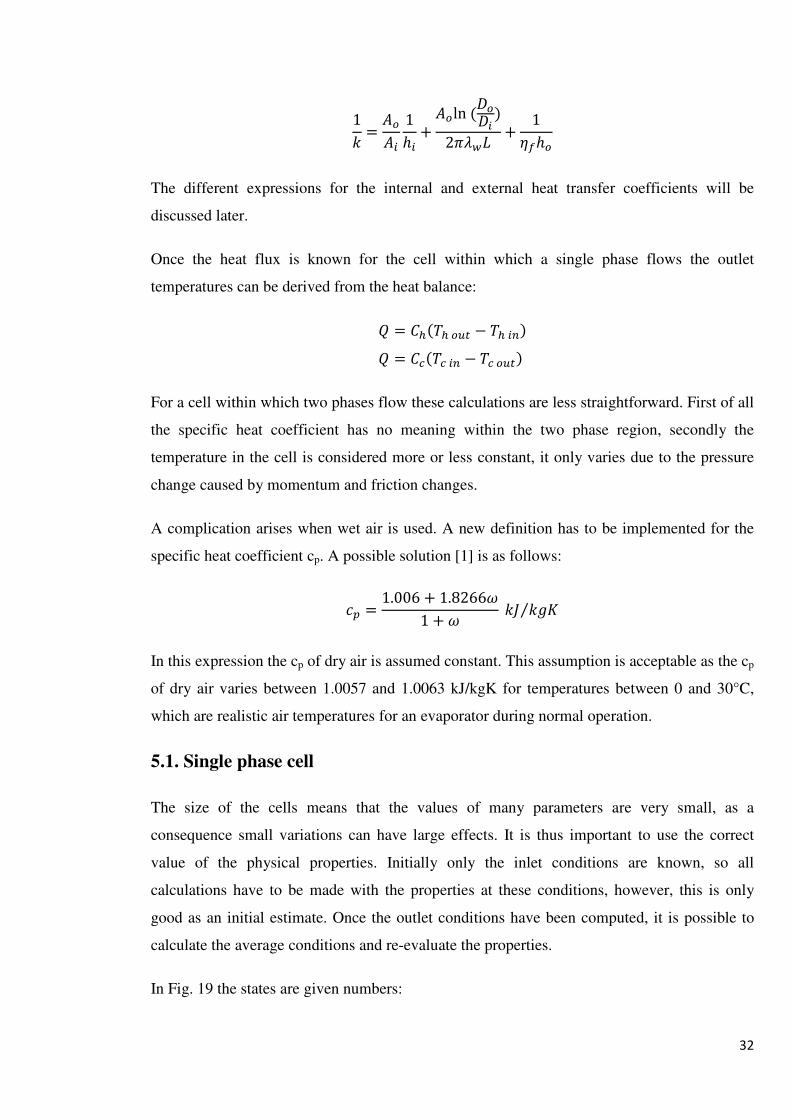
1B � �>��1;� " �>ln J>J� �2KLMN " 1OP;>

The different expressions for the internal and external heat transfer coefficients will be

discussed later.

Once the heat flux is known for the cell within which a single phase flows the outlet

temperatures can be derived from the heat balance:

� � ��� >?@ � ��� � � ��� �� � >?@� For a cell within which two phases flow these calculations are less straightforward. First of all

the specific heat coefficient has no meaning within the two phase region, secondly the

temperature in the cell is considered more or less constant, it only varies due to the pressure

change caused by momentum and friction changes.

A complication arises when wet air is used. A new definition has to be implemented for the

specific heat coefficient cp. A possible solution [1] is as follows:

�� � 1.006 " 1.8266S1 " S BT BUV⁄

In this expression the cp of dry air is assumed constant. This assumption is acceptable as the cp

of dry air varies between 1.0057 and 1.0063 kJ/kgK for temperatures between 0 and 30°C,

which are realistic air temperatures for an evaporator during normal operation.

5.1. Single phase cell

The size of the cells means that the values of many parameters are very small, as a

consequence small variations can have large effects. It is thus important to use the correct

value of the physical properties. Initially only the inlet conditions are known, so all

calculations have to be made with the properties at these conditions, however, this is only

good as an initial estimate. Once the outlet conditions have been computed, it is possible to

calculate the average conditions and re-evaluate the properties.

In Fig. 19 the states are given numbers:

33

Fig. 19: The states

A flow chart of the calculation of a single cell is as follows:

1 2

4

3

5

34

Read ma, mr, Tai and Tri

Determine Ch, Cc and k at States 1 and 3

Calculate NTU and qmax

First estimate of dp

qprevious = q Calculate ε

Calculate q = εqmax

Determine Tao and Tro with q

Calculate average states (5) for the refrigerant and air side and store them in 2

and 4

Calculate dp Determine Ch, Cc and k at states at 5

(stored in 2 and 4)

Recalculate NTU and qmax

xo = 1 or 0 Go to calculation for

two phase flow

XA A��YZ�>?[A X \ �+9:1+9]

Store outlet conditions in 2 and 4

STOP

Fig. 20: Flowchart for single phase cell

no

yes

no

yes

35

The iterations stop when the relative difference between two iterations is smaller than a

certain value (criteria), this value can be chosen. A trade-off has to be made between precision

and calculation time. When the relative difference is set to 1% each cell generally needs 3

iterations, if a precision of 0.01% is needed, 4 iterations are required, this equates in an

increase of calculation time of 33%. However, the extra iteration in fact offers a greater

precision than that of the criteria; it increases to 1.10-3 %.

Case Criteria (%) # of

iterations

Achieved rel. diff.

(%)

Extra comp. time

compared to case 1

1 1 3 1 1

2 0.1 4 0.00001 1.33

3 0.00001 4 0.00001 1.33

4 0.000001 5 0 1.66

Table 1: Influence criteria

For a small heat exchanger the extra computation time is acceptable, but for a large

evaporator with tube-splitting and parallel circuits it may be desirable to accept a lower

precision.

The outlet quality of the cell is determined by means of XProps. If xo is smaller than 1, in

other words the cell contains two phase flow, xo can’t be calculated with the temperature and

the pressure as these two properties do not define a well-defined point under the dome in a P-

h diagram. The outlet enthalpy is needed as is the pressure. The hro is calculated by:

;�> � ;�� A��

36

5.2. Two phase cell

During evaporation the temperature is constant if there is no pressure drop. If there is a

change in pressure this is accompanied by a change in temperature. To calculate the pressure

change within a cell (see later) the inlet and outlet quality is required. However, the outlet

enthalpy can only be determined by the outlet pressure and outlet enthalpy. It is clear that

iterations will be needed to determine the outlet conditions.

Once the heat transfer of the cell has been found with the ε-NTU method with the simplified

equation for ε, the outlet enthalpy can be determined with the same correlation as above. An

initial pressure drop can be made with the assumption that the inlet and outlet conditions are

the same. The outlet quality is then defined by the outlet enthalpy and pressure. A new

calculation of the pressure drop is then possible, followed by the resulting outlet quality and

so on. This is repeated until the relative difference of the outlet quality is reasonably small. A

flow chart for a two phase cell is as follows:

37

no

no

yes

Fig. 21: Flowchart for two phase cell

Determine tao

Recalculate Ch, Tw, k, NTU and qmax

|A A��YZ�>?[�/A| \ �+9:1+9]2

Store outlet conditions in 2 and 4

STOP

Set averages (v, T, p and x) to 2

Read ma, mr, Tai and Tri Set xo to xi

First estimate of Tw

Determine Ch en k

qprevious = q Calculate ε

Calculate q = εqmax

Determine Tao

Calculate average for air side (5) and store it in 4

Calculate NTU and qmax

Calculate hro

xtemp = xo

Calculate dp and determine p at 4

Determine x = f(hro, p)

_%> %@Y���/%>_ \ �+9:1+9]1

38

The temperature is required for the calculation of the heat transfer coefficient on inside of the

tube. The applied correlation will be discussed later. The first estimate of Tw is the average of

the inlet refrigerant temperature and the inlet air temperature.

M � �� " ��2

Once it is known, k can be determined and q computed. The new wall temperature can then be

estimated using the following formula:

A � ��;@�M [�@� M � A��;@� " [�@

The saturation temperature of the refrigerant is resolved at the average of the inlet and outlet

pressure of the cell. The wall temperature can be used to establish if condensation takes place

on the fins and the outside of the tube. This happens when the wall temperature is beneath the

dew point for water vapour.

Again, a trade-off has to be made between computation time and accuracy, for two phase flow

however this is of greater importance due to the fact that two iterations have to be made per

cell. If every value had to be calculated just once, 70 computations would have to be made of

which 7 are for the determination of the outlet conditions. This means that every iteration of

the smallest loop adds 10% to the computation time. However, not every iteration of the

larger loop means the same amount of iterations of the smaller one. As the heat transfer varies

less and less from iteration to iteration, the outlet conditions vary increasingly less too. A few

typical values are given in Table 2, these are for criteria 2 set at 1%. The computation time is

given relative to the time required if no iterations where necessary.

For the influence of criteria2, criteria1 is set to 1%. Typical values are shown in Table 3.

39

Case Criteria1

(%)

Achieved

Rel. diff. (%)

Min. # of

it.

Max. # of

it.

Av. # of it. Comp.

time

1 1 0.01 1 2 1.17 6.1

2 0.1 0.01 1 2 1.67 6.4

3 0.01 0.01 1 2 1.83 6.5

4 0.001 1.10-6 2 2 2 6.6

5 0.0001 1.10-6 2 3 2.17 6.7

Table 2: Influence criteria1

Case Criteria2

(%)

Achieved Rel. Diff.

(%)

# of it. Comp. time Rel. comp.

time

1 1 1 6 6.1 1

2 0.1 0.1 7 7.1 1.164

3 0.01 0.01 8 8.1 1.328

4 0.001 0.001 9 9.1 1.492

Table 3: Influence criteria2

When the precision of the outlet quality is set to 1 % only the first iteration of the larger loop

requires more than one iteration of the smaller loop, thus explaining why the computation

time relative to 1 single run without recursions is the amount of iterations plus 10 %.

REFERENCES

[1] M. Duminil, Air humide, Techniques de l’Ingénieur

40

Chapter 6

Flow and Heat Exchanger Properties

6.1. External Heat Transfer Coefficient

For most practical applications the airside thermal resistance is roughly 5 to 10 times that of

the refrigerant side. Consequently enhanced surfaces are often employed to effectively

improve the overall performance of the fin and tube heat exchanger. One of the very popular

enhanced surfaces is the interrupted surface. This is because interrupted surfaces can provide

higher average heat transfer coefficients owing to periodical renewal of the development of

boundary layer, which acts as insulation for the heat transfer. The most common interrupted

surfaces are offset strip and louver fin (Fig. 22). The louvered fin pattern is more beneficial

when produced in large quantities since it can be manufactured by high speed production

techniques. There are a couple of variants of louver fin heat exchangers as combined with the

tubes.

Fig. 22: Louver Fins

Fig. 23: Louver Fin – Tube Combination

41

Wang proposed a correlation for the heat transfer coefficient on the air side based on a data

bank of 49 samples [1]. The correlation for the Colburn j factor is as follows:

For `1a� \ 1000

b � 14.3117`1a�f� 4g�J�7f� hN�N�ifj 4g�k(7fl 4k(k@7m�.n�l

T1 � 0.991 0.1055 4k(k@7j.� ln hN�N�i

T2 � 0.7344 2.1059 h 6p.qqln`1a�� 3.2i

T3 � 0.08485 4k(k@7ml.l6mp.rs

T4 � 0.1741ln 6� For`1a� t 1000

b � 1.1373`1a�fq 4g�k(7fr hN�N�ifn 4k(k@7fs6p.jqlq

T5 � 0.6027 " 0.02593 4k(J�7p.q�6mp.q3. hN�N�i

T6 � 0.4776 " 0.40774 h 6p.nln `1a�� 4.4i

T7 � 0.58655 4g�J�7�.j6mp.rq 4k(k@7m�.r

T8 � 0.0814ln`1au� 3� J� � 4��N

With Dc the fin collar outside diameter:

42

J� � J> " 2vP

The definition of the Colburn j factor is

b � 6/`1k+�/j

With the Nusselt number:

6/ � ;>J�L>

As a result the external heat transfer coefficient is

;> � b`1k+�/j L>J�

Correlations have also been implemented for forced convection flow across a smooth circular

cylinder as proposed by Gnielinski [2]:

6/(,> � 0.3 " w6/(,(��� " 6/(,@?��

6/(,(�� � 0.664x`1(√k+z

6/(,@?� � 0.037`1(p.sk+1 " 2.443`1(mp.�k+�/j 1� With

3 � J> K2

`1( � �/�3{

6/( � ;>3L

um = free-stream velocity, all properties at fluid bulk mean temperature. This correlation is

valid over the ranges 10 < Rel < 107 and 0.6 < Pr < 1000.

43

6.2. Internal heat transfer coefficient

As mentioned before different correlations are used for single phase flow and two phase flow.

When only one phase is present in the tube, the Nusselt number can be used, which is

internally:

6/� � ;�J�L�

The Nusselt number can also be determined by one of the following equations provided by

Wielandt depending on the internal diameter of the tube:

For Di = 0.007m:

6/� � 0.0329`1p.s�k+p.lq

For Di = 0.008m:

6/� � 0.0325`1p.s�k+p.lq

For Di = 0.00952m:

6/� � 0.0315`1p.s�k+p.lq

The internal heat transfer coefficient can easily be determined using the two equations.

For the heat transfer coefficient for two phase flow information can be found in the

Engineering Data Book by Wolverine Tube Inc. [3]. Different methods are discussed.

The local two phase boiling heat transfer coefficient for evaporation inside a tube htp is

defined as

;@� � AM�(( [�@� Where q corresponds to the local heat flux from the tube wall into the fluid, Tsat is the local

saturation temperature at the local saturation pressure psat and Twall is the local wall

temperature at the axial position along the evaporator tube, assumed to be uniform around the

44

perimeter of the tube. There are two heat transfer mechanisms that are dominant in most flow

boiling models: nucleate boiling heat transfer (hnb) and convective boiling heat transfer (hcb).

Nucleate boiling under these conditions is similar to nucleate pool boiling except for any

effect of the bulk flow on the growth and departure of the bubbles and the bubble induced

convection process. The bubbles formed inside a tube may slide along the heated surface due

to the axial bulk flow, and hence the micro-layer evaporation process underneath the growing

bubbles may also be affected. Convective boiling refers to the convective process between the

heated wall and the liquid phase. For instance, for annular flow without nucleate boiling in the

liquid film, the convective heat transfer process can be envisioned as single phase force

convection across the film with evaporation taking place at the liquid-vapour interface of the

central core.

Different flow boiling models can be compared by the way they combine the two heat transfer

coefficients to obtain htp. Nucleate boiling tends to be dominant at low vapour qualities and

high heat fluxes while convection tends to dominate at high vapour qualities and mass

velocities and low heat fluxes. For intermediate conditions, both mechanisms are often

important.

In most models the nucleate boiling coefficient is determined utilizing a nucleate pool boiling

correlation from the literature or by proposing a new nucleate boiling term as part of the flow

boiling correlation. Likewise, the convective heat transfer coefficient is often related to what

is sometimes referred to as the liquid only heat transfer coefficient hL, which is determined

with a single phase turbulent flow heat transfer correlation, usually that of Dittus-Boelter [4].

Furthermore, these methods assume that the liquid fraction flowing in the channel, �' 1 %�, occupies the entire cross-section of the channel in the calculation of hL.

Gungor and Winterton [5] put together a large database of 3693 points from literature for

mostly vertical upflows and some vertical downflows. Their local two phase flow boiling

coefficient htp is the sum of the nucleate boiling contribution hnb and the convective

contribution hcb, where their basic equation is

;@� � |;} " �;�~

hL is calculated from the Dittus-Boelter correlation using the local liquid fraction of the

flow �' 1 %�:

45

;} � 0.023`1}p.sk+}p.l 4L}J�7

`1} � �' 1 %�J�{}

k+} � ��}{}L}

While their nucleate pool boiling coefficient is obtained with the Cooper [6] nucleate pool

boiling equation:

;�~ � 55��p.�� 0.4343 ln����mp.qq�mp.qAp.rn

The above equation is dimensional and gives the heat transfer coefficient in W/m2K. The heat

flux q must be introduced in W/m2. M is the molecular weight and pr is the reduced pressure,

which is the ratio of the saturation pressure psat to the critical pressure pcrit. Their two phase

convection multiplier E is a function of the Martinelli parameter and also the heat flux via the

Boiling number:

| � 1 " 24000�,�.�r " 1.37 4 1�@@7p.sr

�@@ � 41 %% 7p.� 4���}7p.q 4{}{�7p.�

�, � A�' ;}�

The boiling suppression factor S is

� � C1 " 0.00000115|�`1}�.�nGm�

Compared to their database, this method gave a mean deviation of ±21.4% compared to

±57.7% for the Chen correlation [7] and ±21.9% for the Shah correlation [8]. Hence, as the

Shah correlation was not developed using this database, this comparison gives a good

independent credibility of its accuracy. Using the same equivalent diameter definition as

Shah, Gungor-Winterton predicted evaporation in vertical annuli to a mean error of ±29.4%.

46

The method developed by Gungor –Winterton was based on vertical tubes. Adjustments are

needed to be able to apply the correlations for the vertical tubes to horizontal ones. They set a

threshold between stratified and non-stratified flow using the liquid Froude number FrL

defined as:

g+} � �' ��}�UJ� Their threshold value was set at FrL < 0.05. When FrL >0.05 their vertical tube method is used

without change but when FrL < 0.05, their factor E is corrected as follows

|� � g+}p.�m����� Thus, the new parameter E2 is applied as a multiplier to E in their method. Their boiling

suppression factor S, is similarly multiplied by another correction factor

�� � g+}�/�

These two corrections have the tendency to reduce the two-phase flow boiling heat transfer

coefficient at low mass velocities but leaves them unchanged at large mass velocities.

The correlations for the heat transfer coefficient contain the local heat flux q, because q

determines the boiling time. This causes a problem due to the fact that q is initially unknown

so the first calculation of htp isn’t possible. However, algebra offers a solution. Combining the

correlations a non-linear equation in htp can be written, which can be solved iteratively using

the Newton-Raphson technique.

Lemma:

If f and g are continuous functions on a closed interval I, and if U%� � 0 for all x � I, then

the equations 2%� � % and �%� � 0 with

�%� � % 2%�U%� Have the same solutions in the interval I, i.e., the two equations are equivalent.

Newton-Raphson’s technique:

47

If 2 � ��C], 0G has a simple root ξ in (a,b), then 2�� � 0 and 2��� � 0. Using the above

mentioned lemma with U%� � 1/2�%�, the iteration function � becomes

�%� � % 2%�2�%� And the iteration rule is given as

%�� � ��%�m��� � %�m�� 2�%�m���2�%�m��� 2,+ � � 1,2, …

Fig. 24: Newton’s Technique

Since ���� � 0, the procedure converges at least quadratically by the theorem in Appendix

A.

To be able to apply this method to the Gungor-Winterton correlation an equation has to be

found for which 2�;@�� � 0.

;@� � |;} " �;�~

Replace E and S:

;@� �41 " 24000�,�.�r " 1.37 � �����p.sr7 ;} "h�1 " 0.00000115 41 " 24000�,�.�r " 1.37 � �����p.sr7� `1}�.�n�m�i;�~

48

Substitute hnb:

;@� �

41 " 24000�,�.�r " 1.37 � �����p.sr7 ;} "h�1 " 0.00000115 41 " 24000�,�.�r " 1.37 � �����p.sr7� `1}�.�n�m�i55��p.�� 0.4343 ln����mp.qq�mp.qAp.rn

Substitute Bo and q:

;@� �

h1 " 24000 4;:��-]33 8]:��' ;N� 7�.�r " 1.37 � �����p.sri;} "��1 " 0.00000115 h1 " 24000 4;:��-]33 8]:��' ;N� 7�.�r " 1.37 � �����p.sri� `1}�.�n�

m��

55��p.�� 0.4343 ln����mp.qq�mp.q 4;:�-]33 8]:��' ;N� 7p.rn

The equation f(htp) is thus:

2;@�� �

h1 " 24000 4;:��-]33 8]:��' ;N� 7�.�r " 1.37 � �����p.sri;} "��1 " 0.00000115 h1 " 24000 4;:��-]33 8]:��' ;N� 7�.�r " 1.37 � �����p.sri� `1}�.�n�

m�� <

h55��p.�� 0.4343 ln����mp.qq�mp.q 4;:�-]33 8]:��' ;N� 7p.rni ;@�

The derivative of this function is then:

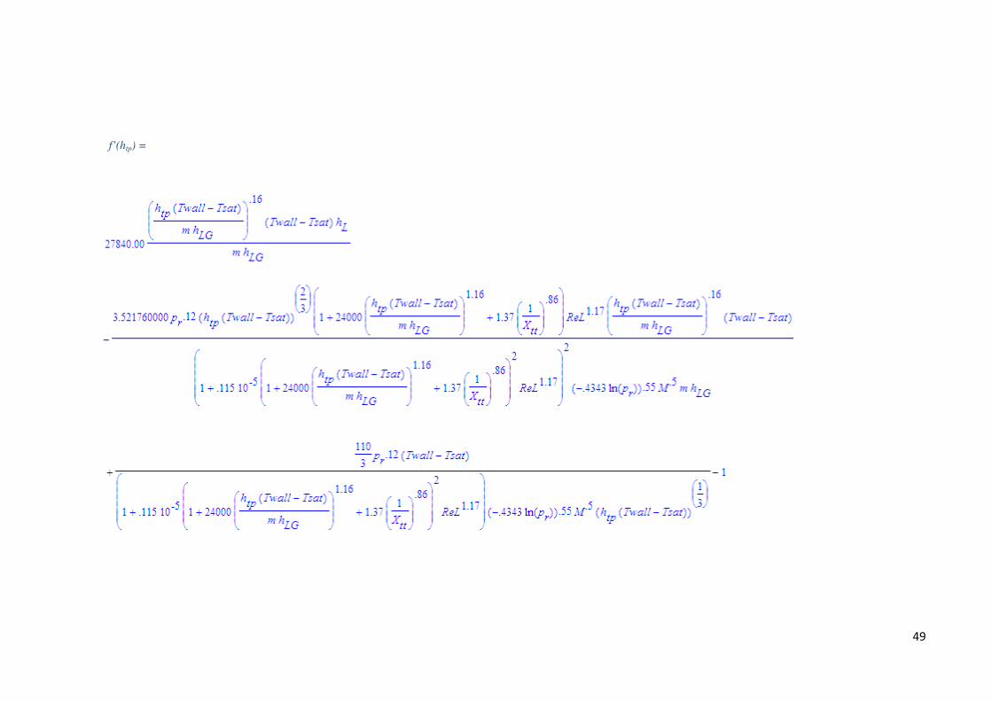
49

f’(htp) =

50

The wall temperature present in the equation is the average of the air and refrigerant inlet

temperature as at the point of calculation no other information is available. Once the internal

heat transfer coefficient is determined, q can be calculated and used in the next iteration for

the computation of htp, Newton-Raphson is not necessary anymore.

6.3. Fin efficiency

The final parameter to be established in the equation for k is the fin efficiency. It is defined as

the ratio of the actual heat transfer from an extended surface to the maximum possible heat

transfer from the surface. The maximum heat transfer would occur if the temperature of the

extended surface were equal to the base temperature at all points.

Fin and tube heat exchangers are generally composed of continuous plate fins. The fins are

metal sheets pierced through by the tube bank. The tube lay-out is in inline or staggered

configuration (Fig. 25). In order to express the fin efficiency of such continuous plate fins, the

fin is divided in unit cells. The considered fin shape is rectangular for the inline configuration

and hexagonal for the staggered lay-out.

Fig. 25: Unit cells for inline and staggered tube layouts with plain plate fins

Several studies have been performed in order to simplify the circular fin efficiency

formulation by avoiding the use of modified Bessel functions. Among all the approximations,

the Schmidt approximation [9] is the most widely used one. Hong and Webb [10] propose to

slightly modify the Schmidt equation in order to obtain better accuracy. They suggest:

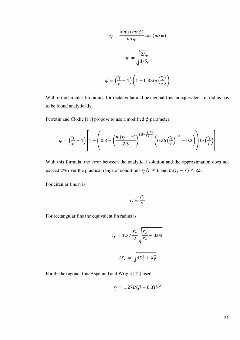
51

OP � tanh �+���+� cos �+�� � � ¡2;>LPvP

� � �+P+ 1� h1 " 0.353. �+P+ �i

With rf the circular fin radius, for rectangular and hexagonal fins an equivalent fin radius has

to be found analytically.

Perrotin and Clodic [11] propose to use a modified � parameter.

� � �+P+ 1� ¢1 " £0.3 " h�+P +�2.5 i�.qm ����¤� h0.26 �+P+ �p.j 0.3i¥ 3. �+P+ �¦ With this formula, the error between the analytical solution and the approximation does not

exceed 2% over the practical range of conditions +P + § 6⁄ and �+P +� § 2.5.

For circular fins rf is

+P � g�2

For rectangular fins the equivalent fin radius is

+P � 1.27�2̈ ¡�a�¨ 0.03

2�a � w4�}� " ��̈

For the hexagonal fins Aspelund and Wright [12] used:

+P � 1.27�© 0.3��/�

52

© � ª�

� � �( 92 �( \ �@2 , ,:;1+-981 � � �@/2

ª � 12¡4�@2 7� " �(�

In Schmidt’s study it is claimed that the approximation is limited to situations where β > 1.

Zeller & Grewe [13] give an improved equation for the equivalent circular fin radius based on

the relative perimeters of the circle and the hexagon. The relation for the equivalent radius, as

defined by Zeller & Grewe is:

+P � k�Y�2K

Where Phex is the perimeter of the hexagonal fin:

k�Y� � 4«� " 2«�

Fig. 26: Geometry hexagonal fin

53

REFERENCES

[1] C.C. Wang, C.T. Chang et al., Heat transfer and friction correlation for compact

louvered fin-and-tube heat exchangers, International Journal of Heat and Mass Transfer 42 (1999) pp. 1945-1956

[2] V. Gnielinski, New equations for heat transfer and mass transfer in turbulent pipe and

channel flow, Int. Chem. Eng. 16 2 (1976) pp. 359–368

[3] K.J. Bell and A.C. Mueller, Wolverine Engineering Data Book III (2001)

[4] E.J. Dittus and L.M.K. Boelter, Publications on Engineering Vol. 2, (1930) pp. 443

[5] K.E. Gungor and R.H.S. Winterton, A general correlation for Flow-Boiling in Tubes

and Annuli, International Journal of Heat and Mass Transfer 29 (1986) pp. 351-358

[6] M.K. Cooper, Advances in Heat Transfer Vol. 16, (1984) pp. 157-159

[7] J.C. Chen, A correlation for boiling heat transfer of saturated fluids in convective

flows, Ind. Eng. Chem. Process Des. Dev. Vol. 5, (1966) pp. 322-329

[8] M.M. Shah, Chart correlation for saturated boiling heat transfer: Equations and

further study, ASHRAE Trans. Vol. 88, (1982) pp. 185-196

[9] T.E. Schmidt, Heat transfer calculation for extended surfaces, Refrigerating Engineering Vol. 57, (1949) pp. 351-357

[10] K.T. Hong and R.L. Webb, Calculation of fin efficiency for wet and dry fins, HVAC&R Research Vol. 2, (1996) pp.27-41.

[11] T. Perrotin and D. Clodic, Fin Efficiency Calculation In Enhanced Fin-And-Tube Heat

Exchangers In Dry Conditions, International Congress of Refrigeration, (2003) paper ICR0026

[12] K.A. Aspelund, Optimization of Plate-Fin-and-Tube Condenser Performance and

Design for Refrigerant R-410A Air-Conditioner, M.S. Thesis Georgia Institute of Technology, (2001)

[13] M. Zeller and M. Grewe, A Generalized Approximation Equation for the Efficiency of

Fins on Circular and Elliptic Tubes, Thermo and Fluid Dynamics Vol. 29, (1994) pp. 379-382

54

Chapter 7

The Refrigerant Pressure drop

7.1. Single Phase Flow

By means of dimensional analysis the pressure drop for single phase flow can be derived:

∆� � 2 NJ��*�2

With f the fanning friction factor, this factor is dependent on the Reynolds number. Different

correlations exist for laminar and turbulent flow.

Laminar:

2 � 16`1

For turbulent the Blasius correlation is used, which is valid between 4000 and 105 Re:

2 � 0.079`1mp.�q

7.2. Two Phase Flow

For two phase flow the total pressure drop of a fluid is the sum of the variation of potential

energy of the fluid, kinetic energy of the fluid and that due to friction on the channel walls.

Thus, the total pressure drop ∆ptotal is the sum of the static pressure drop (elevation head)

∆pstatic, the momentum pressure drop (acceleration) ∆pmom, and the frictional pressure drop

∆pfrict:

∆�@>@�( � ∆�[@�@�� " ∆��>� " ∆�P���@ For a horizontal tube, there is no change in static head so ∆pstatic = 0. The momentum pressure

drop reflects the change in kinetic energy of the flow and is:

∆��>� � �� ¬� 1 %���}1 �� " %�����>?@ � 1 %���}1 �� " %�������­

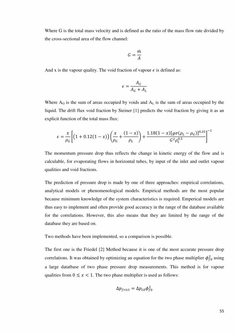
55

Where G is the total mass velocity and is defined as the ratio of the mass flow rate divided by

the cross-sectional area of the flow channel:

� � �'�

And x is the vapour quality. The void fraction of vapour � is defined as:

� � ���� " �}

Where AG is the sum of areas occupied by voids and AL is the sum of areas occupied by the

liquid. The drift flux void fraction by Steiner [1] predicts the void fraction by giving it as an

explicit function of the total mass flux:

� � %�� ��1 " 0.121 %�� h %�� " 1 %��} i " 1.181 %�CU®�} ���Gp.�q���}p.q �m�

The momentum pressure drop thus reflects the change in kinetic energy of the flow and is

calculable, for evaporating flows in horizontal tubes, by input of the inlet and outlet vapour

qualities and void fractions.

The prediction of pressure drop is made by one of three approaches: empirical correlations,

analytical models or phenomenological models. Empirical methods are the most popular

because minimum knowledge of the system characteristics is required. Emperical models are

thus easy to implement and often provide good accuracy in the range of the database available

for the correlations. However, this also means that they are limited by the range of the

database they are based on.

Two methods have been implemented, so a comparison is possible.

The first one is the Friedel [2] Method because it is one of the most accurate pressure drop

correlations. It was obtained by optimizing an equation for the two phase multiplier �Pp� using

a large datatbase of two phase pressure drop measurements. This method is for vapour

qualities from 0 § % \ 1. The two phase multiplier is used as follows:

∆�P���@ � ∆�}p�Pp�

56

With

∆�}p � 42}p 4 NJ�7�� 4 12�}7

Where

2}p � 0.079`1}pp.�q ].¯ `1}p � �J�{}

Friedels multiplier is correlated as:

�Pp� � | " 3.24gªg+°p.plq±1}p.pjq

Where FrH, E, F and H are as follows:

g+° � ��UJ���

| � 1 %�� " %� �}2�p��2}p

g � %p.ns1 %�p.��l

ª � 4�}��7p.�� 4{�{}7p.�� 41 {�{}7p.n

The liquid Weber number WeL is defined as:

±1} � ��J�®��

And Friedels definition of the homogeneous density ρh is:

�� � 4 %�� " 1 %�} 7m�

The correlation is applicable to vertical up flow and to horizontal flow. This method is known

to work well when the ratio µL/µG < 1000, which is the case for most working fluids in

operation conditions. For R22 for example the ratio ranges between approximately 14 and 22.

57

The second implemented method is that of Grönnerud [3], which was specifically developed

for refrigerants and is as follows:

Δ�P���@ � �&³Δ�}p

∆pL0 is as before and the two phase multiplier is

�&³ � 1 " 4¯�¯«7�� ¢ ��}����{}{��p.�q 1¦ The frictional pressure gradient depends on the Froude number and is:

4¯�¯«7�� � 2��C% " 4%�.s %�p2��p.q�G If the liquid Froude number g+} t 1, then the friction factor fFr =1.0, or if g+} § 1, then:

2�� � g+}p.j " 0.0055 43. 1g+}7�

Where

g+} � ��UJ��}�

The correlation of Grönnerud is applicable to vapour qualities from 0 ≤ x < 1.

Moreno Quibén and Thome [4] compared experimental results from three different

refrigerants and a wide range of operating conditions to three leading methods (Friedel,

Grönnerud, Müller-Steinhagen and Heck [5]). They showed that all three provided a

reasonable agreement at one of the mass velocities studied, but they either significantly over

predicted or under predicted the data at the other mass velocities. Furthermore, the methods

didn’t accurately relate the variation in two-phase frictional pressure drop and vapour quality.

Despite these shortcomings, the Grönnerud method was found to provide the most accurate

predictions.

58

REFERENCES

[1] D. Steiner, VDI-Wärmeatlas (VDI Heat Atlas), chapter Hbb. Verein Deutscher Ingenieure VDI-Gessellschaft Verfahrenstechnik und Chemieingenieurwessen (GCV), (1993)

[2] L. Friedel, Improved friction drop correlations for horizontal and vertical two-phase

pipe flow, European Two-phase Flow Group Meeting (1979)

[3] R. Gronnerud, Investigation of liquid hold-up, flow-resistance and heat transfer in

circulation type of evaporators, In Annexe 1972-1, Bull. de l’Inst. du Froid (1979)

[4] J. Moreno-Quiben and J. R. Thome, Two-phase pressure drops in horizontal tubes:

new results for R-410A and R-134a compared to R-22, International Congress of Refrigeration, (2003), paper IIC00

[5] H.Müller-Steinhagen and K.Heck, A simple friction pressure correlation for two-

phase flow in pipes, Chem. Eng. Process 20, (1986) pp.297–308

59

Chapter 8

Heat Exchanger calculations

8.1. Tube calculations

The tubes are uniformly divided into cells; the amount of cells has an influence on the

accuracy. For evaporators, however, quantity of elements has to be sufficiently large so that

the assumptions made for the calculations are valid. For example the simplified ε correlation

is only applicable if there is nearly no temperature variation. If the elements are too long, the

effect of the pressure drop through the element and the related temperature decrease will

make the correlation less accurate. For a tube of 410 mm 25 elements are adequate, every

element is then 16.4 mm long. A typical value, using the correlation of Friedel, for the

pressure drop in the two phase region is 20 Pa, this corresponds with a change in temperature

of approximately 0.001°C. These are acceptable values.

Not every tube has the same flow direction. If the flow in a certain tube is for instance from

left to right when looking at the heat exchanger from the direction of the airflow, the flow in

the next tube must be from right to left. The tubes are connected by bends. The direction is of

importance during calculations because the right elements of the matrix of the refrigerant

states and the air states have to be used. When a tube is run through from the inlet to the other

end, the elements of the matrix are used in ascending order, in the other direction in

descending order.

As can be seen in the flow chart for a single cell, the outlet states are stored in as inlet states

for the next cell, for that reason an extra refrigerant state is added at the end of the tube so that

the last element of the tube can also be calculated.

The calculations for a tube are represented in a flow chart:

60

Fig. 27: Flow chart for tube

The direction from inlet to the other end is chosen as 1 the other direction is then -1. If a tube

follows a tube with direction 1 in the flow path, the direction of that tube is -1. In other words,

the tubes along a flow path have alternating directions.

8.2. Heat exchanger simulation

The calculation methods for the tubes and cells have been discussed as has the determination

of the computation sequence of the tubes. However, a certain topic that is vital for the

simulations has not been discussed, namely tube splitting.

Tube splitting, as mentioned before, is present to reduce the pressure drop on the refrigerant

side and optimize the heat transfer. When a split is encountered, the refrigerant mass flow

does not just simply part into two equal mass flows in both tubes. The flow is apportioned; the

apportionment of refrigerant flow at a split is such that the downstream pressure drops of the

yes

yes

no

no xi = 0 or 1

Calculations single phase cell

Calculations two phase

cell

i = 0

Stop

Number of cells n

Direction = 1 i = n

i = 0

xi = 0 or 1

Calculations single phase cell

Calculations two phase

cell

i = n

Stop

no

yes

yes

yes

no

no

i = i - 1 i = i + 1

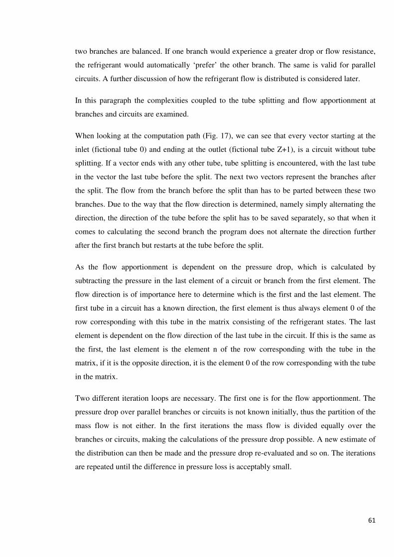
61

two branches are balanced. If one branch would experience a greater drop or flow resistance,

the refrigerant would automatically ‘prefer’ the other branch. The same is valid for parallel

circuits. A further discussion of how the refrigerant flow is distributed is considered later.

In this paragraph the complexities coupled to the tube splitting and flow apportionment at

branches and circuits are examined.

When looking at the computation path (Fig. 17), we can see that every vector starting at the

inlet (fictional tube 0) and ending at the outlet (fictional tube Z+1), is a circuit without tube

splitting. If a vector ends with any other tube, tube splitting is encountered, with the last tube

in the vector the last tube before the split. The next two vectors represent the branches after

the split. The flow from the branch before the split than has to be parted between these two

branches. Due to the way that the flow direction is determined, namely simply alternating the

direction, the direction of the tube before the split has to be saved separately, so that when it

comes to calculating the second branch the program does not alternate the direction further

after the first branch but restarts at the tube before the split.

As the flow apportionment is dependent on the pressure drop, which is calculated by

subtracting the pressure in the last element of a circuit or branch from the first element. The

flow direction is of importance here to determine which is the first and the last element. The

first tube in a circuit has a known direction, the first element is thus always element 0 of the

row corresponding with this tube in the matrix consisting of the refrigerant states. The last

element is dependent on the flow direction of the last tube in the circuit. If this is the same as

the first, the last element is the element n of the row corresponding with the tube in the

matrix, if it is the opposite direction, it is the element 0 of the row corresponding with the tube

in the matrix.

Two different iteration loops are necessary. The first one is for the flow apportionment. The

pressure drop over parallel branches or circuits is not known initially, thus the partition of the

mass flow is not either. In the first iterations the mass flow is divided equally over the

branches or circuits, making the calculations of the pressure drop possible. A new estimate of

the distribution can then be made and the pressure drop re-evaluated and so on. The iterations

are repeated until the difference in pressure loss is acceptably small.

62

The second iteration is for the total heat transfer. As the outlet conditions of the air are

unknown, the inlet conditions of the next row of tubes are unknown too. Therefore, the outlet

states are initially set to the same values as the inlet states and the inlet conditions of the next

row are a combination of these outlet states. If, for example, the first tube of a circuit is in the

second row of tubes, it will be calculated with (a combination of) the inlet conditions and not

with the true outlet states of the tubes directly in front of the tube in question. Once all tubes

have been calculated once and a second iteration starts, the first tube will then be analyzed

with the proper inlet conditions. The iterations are repeated until the difference in total heat

transfer is small enough.

A flow chart for the heat exchanger is given below:

63

Flow Chart 2

dirtemp = dir

Last Vector ?

∆p over every circuit within margin

mc = D.m

Determine air inlet conditions

Solve tube

Last tube of vector ?

Set inlet first cell of next tube

Set inlet first tubes of the next two vectors

c = the number of parallel circuits

Distribution D = 1/c

Vector 1

Last tube in vector ≠ outlet

Flow Chart 3

Tube 1 Direction dir = 1

Recalculate distribution

Stop

no

no

no

no

yes

yes

yes

yes

Next tube dir = -dir

Next vector

Fig. 28: Flow chart for heat exchanger with complex geometry

64

Stop

Second vector after split Tube 1

mb = (1-d).mt

Determine air inlet conditions

Solve tube

Last tube of vector ?

Set inlet first cell of next tube

∆p over both branches within margin

Recalculate distribution

Distribution d = 1/2

dir = dirtemp

First vector after split Tube 1

mb = d.mc

Determine air inlet conditions

Solve tube

Last tube of vector ?

Set inlet first cell of next tube

no

yes

no

yes

yes

no

Next tube dir = -dir

Next tube dir = -dir

Fig. 29: Flow chart 2 for heat exchanger with complex geometry

65

One iteration loop is not shown in flow chart 1 and this to preserve the clarity. Once the flow

distribution has correctly been determined, the whole process is restarted, however with the

distribution kept the same as in the last iteration so that it doesn’t have to be determined

again. This loop is repeated until the simulated total heat transfer between two consecutive

iterations is sufficiently small. This is not strictly necessary when parallel circuit are

encountered because the air states have been adjusted in the iterations for the flow

apportionment. It has, however, to be implemented for situations where only one circuit is

present.

In the first flow chart it is checked whether a split is present in the circuit or not, if there is,

the part of the circuit before the split is calculated in flow chart 1 and the two branches in flow

chart 2. If there is no split present in the circuit, the computations are down in flow chart 3.

The manner in which the distribution is determined is discussed in the next paragraph. m, mc

and mb are respectively the mass flow entering the heat exchanger, the mass flow in the circuit

and the mass flow in the branch.

Fig. 30: Flow chart 3 for heat exchanger with complex geometry

Next tube dir = -dir

no

yes

Tube 1 Direction dir = 1

mc = D.m

Determine air inlet conditions

Solve tube

Last tube of vector ?

Set inlet first cell of next tube

Stop

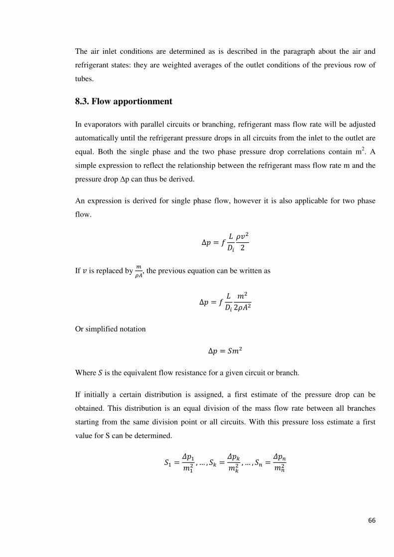
66

The air inlet conditions are determined as is described in the paragraph about the air and

refrigerant states: they are weighted averages of the outlet conditions of the previous row of

tubes.

8.3. Flow apportionment

In evaporators with parallel circuits or branching, refrigerant mass flow rate will be adjusted

automatically until the refrigerant pressure drops in all circuits from the inlet to the outlet are

equal. Both the single phase and the two phase pressure drop correlations contain m2. A

simple expression to reflect the relationship between the refrigerant mass flow rate m and the

pressure drop ∆p can thus be derived.

An expression is derived for single phase flow, however it is also applicable for two phase

flow.

∆� � 2 NJ��*�2

If * is replaced by �́µ, the previous equation can be written as

∆� � 2 NJ���2���

Or simplified notation

∆� � ���

Where � is the equivalent flow resistance for a given circuit or branch.

If initially a certain distribution is assigned, a first estimate of the pressure drop can be

obtained. This distribution is an equal division of the mass flow rate between all branches

starting from the same division point or all circuits. With this pressure loss estimate a first

value for S can be determined.

�� � ¶����� , … , �· � ¶�·�·� , … , �� � ¶�����

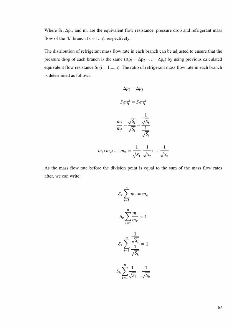
67

Where Sk, ∆pk, and mk are the equivalent flow resistance, pressure drop and refrigerant mass

flow of the ‘k’ branch (k = 1..n), respectively.

The distribution of refrigerant mass flow rate in each branch can be adjusted to ensure that the

pressure drop of each branch is the same (∆p1 = ∆p2 =…= ∆pn) by using previous calculated

equivalent flow resistance Si (i = 1,...,n). The ratio of refrigerant mass flow rate in each branch

is determined as follows:

∆�� � ∆�¸ ����� � �̧ ��̧

���¸ � x�̧x�� �1x��1x�̧

��:��: … :�� � 1x�� : 1x�� : … : 1x��

As the mass flow rate before the division point is equal to the sum of the mass flow rates

after, we can write:

v·º����»� � �·

v·º���·��»� � 1

v·º1x��1x�·

��»� � 1

v·º 1x����»� � 1x�·

68

v· �1x�·∑ 1x����»�

Where δk is the ratio of the refrigerant mass flow rate in the ‘k’ branch or circuit to the total

refrigerant mass flow rate mtotal.

This is not necessarily the quickest converging solution. In single phase flow for example the

factor S also contains a factor which is dependent on the mass flow rate, namely f, the fanning

factor. The fanning factor is calculated with the Re0.25, thus v0.25 is present, this is however

negligible compared to v2.

For two phase flow the term G, defined as �µ , is present in both the momentum and the

frictional pressure drop. The above derivation is thus also applicable. The fact that there are

two phase complicates the matter slightly. In this model it is presumed that the vapour quality

is the same in all parallel circuits or branches, hereby neglecting the effect of gravity on the

liquid and vapour.

Another possible solution is based on the pressure drop correlations proposed by Pierre [1].

v· � �·�@>@�( � º½ 1`· `�⁄ �p.qn�¾��»�

Where `· � ∆�· �·�.nq⁄ is the flow resistance for a given circuit or branch for which v· is

calculated, and `� � ∆�� ���.nq⁄ represents the flow resistance for each circuit or branch

meeting in a given split. This equation was derived by Domanski [2] for the Pierre pressure

drop correlation.

REFERENCES

[1] B. Pierre, Flow Resistance with Boiling Refrigerants, ASHRAE Journal, (1964)

[2] J. Lee and P.A. Domanski, Impact of air and refrigerant maldistributions on the

performance of finned-tube evaporators with R-22 and R-407C (1997)

69

Chapter 9

Model validation

9.1. Water-air

In order to validate the model, tests were run for a heat exchanger within which water flows

as the hot fluid and air passes over as the cold fluid. These are obviously not the normal

operating conditions for an evaporator, but they do give an idea of the correctness of the

single phase flow heat transfer and pressure drop, the flow apportionment and the program

used to determine the fluid properties XProps.

Tests were run at different air side Reynolds numbers, for both uniform and non-uniform air

distribution.

The evaporator geometry is as follows:

3 rows of 14 copper tubes, staggered and row pitch = 12 mm

Do = 7 mm

Di = 6.3 mm

L = 1.15 m

Aluminum fins

Fh = 21 mm

Fp = 17.48 mm

Ft = 0.115 mm

The three rows of tubes are all connected separately to the inlet and the outlet, in other words

they form three parallel circuits, so flow apportionment in necessary.

70

9.1.1. Uniform air distribution

The test conditions are given in table 4.

in

in in

out out out

Fig. 31 : Geometry of heat exchanger

71

Case Tai (°C) Patm (Pa) ma (kg/s) Twi (°C) mw (kg/s) ∆Ta (°C) Tao (°C)

1 19.24 100000 0.223138 60.23 0.173486 36.57 55.80

2 19.26 100000 0.340834 59.45 0.165123 32.50 51.76

3 19.65 100000 0.457320 59.30 0.160932 28.80 48.45

4 19.97 100000 0.687761 58.29 0.146324 21.86 41.83

5 21.33 100000 0.915454 59.20 0.133112 17.60 38.94

6 21.83 100000 1.126399 56.89 0.139631 13.77 35.60

7 20.97 101100 0.232407 51.14 0.182389 26.98 47.95

8 21.01 101100 0.346301 51.44 0.176634 24.65 45.66

9 21.17 101100 0.459504 51.28 0.172117 21.63 42.80

10 21.33 101100 0.579979 51.32 0.170494 19.49 40.82

11 21.38 101100 0.696164 51.51 0.177646 18.16 39.55

12 21.35 101100 0.812415 51.66 0.178607 16.59 37.94

13 21.35 101000 0.926427 51.55 0.175653 15.22 36.58

14 21.32 101000 1.037080 51.38 0.175945 14.06 35.38

15 21.13 101000 1.145666 51.22 0.175689 13.35 34.48

16 18.75 101000 0.579493 67.59 0.148429 30.32 49.07

17 20.00 101000 0.809457 60.14 0.158941 21.18 41.18761

18 20.59 101000 1.038373 60.41 0.159705 18.24 38.82522

Table 4: Test Conditions for water-air

3 series of test were run, each with constant refrigerant inlet conditions but with varying air

side inlet conditions. The simulations results are given in table 5.

72

Test SimulatonSimulation

with XPropsTest Simulaton

Simulation with XProps

Case Re (-) Tao (°C) Tao (°C) Tao (°C) Q (W) Q (W) Q (W)

1 253 55.80 55.82 55.88 8217.7 8222.7 8235.2

2 386 51.76 50.98 51.05 11155.9 10885.0 10910.5

3 517 48.45 47.39 47.48 13263.7 12775.8 12814.8

4 777 41.83 41.04 41.13 15137.7 14592.5 14652.5

5 1031 38.94 37.96 38.04 16224.9 15319.3 15398.4

6 1267 35.60 35.46 35.53 15612.3 15454.6 15539.7

7 262 47.95 47.81 47.84 6314.7 6281.5 6289.7

8 390 45.66 45.19 45.24 8596.3 8433.5 8449.8

9 518 42.80 42.56 42.61 10008.7 9895.6 9920.0

10 653 40.82 40.42 40.47 11381.8 11145.0 11177.3

11 784 39.55 39.06 39.11 12730.9 12388.4 12427.0

12 915 37.94 37.69 37.74 13569.1 13365.8 13410.3

13 1043 36.58 36.30 36.35 14198.4 13939.2 13989.6

14 1168 35.38 35.18 35.24 14676.4 14475.5 14529.2

15 1291 34.48 34.12 34.17 15391.2 14977.6 15036.1

16 657 49.07 48.52 48.59 17694.4 17372.8 17412.4

17 915 41.19 40.73 40.80 17263.3 16893.4 16946.7

18 1172 38.83 38.16 38.22 19067.0 18369.9 18438.4

Table 5: Simulation Results

In all cases but one (namely case 1) XProps gives results closer to the test values. In Table 6

the relative difference between the test results and the simulation results are given.

73

Simulaton without Xprops

Simulation with

XProps

Case Re (-) RD (%) RD (%)

1 253 0.06 0.21

2 386 -2.43 -2.20

3 517 -3.68 -3.38

4 777 -3.60 -3.21

5 1031 -5.58 -5.09

6 1267 -1.01 -0.46

7 262 -0.53 -0.40

8 390 -1.89 -1.70

9 518 -1.13 -0.89

10 653 -2.08 -1.80

11 784 -2.69 -2.39

12 915 -1.50 -1.17

13 1043 -1.83 -1.47

14 1168 -1.37 -1.00

15 1291 -2.69 -2.31

16 657 -2.08 -1.80

17 915 -2.14 -1.83

18 1172 -3.66 -3.30

Table 6: The relative difference between simulation en test results

The simulation results are all within ±5% of the test results, which is a good outcome. This is

shown in Fig. 32. The improvement achieved by XProps is in the region of 0.3%.

0

2000

4000

6000

8000

10000

12000

14000

16000

18000

20000

0

Qsi

m[W

]

0

2000

4000

6000

8000

10000

12000

14000

16000

18000

20000

0

Qsi

m[W

]

Fig. 32: Simulation results vs. Test results

Fig. 33: Simulation results with XProps vs. Reynolds number

5000 10000 15000

Qtest [W]

200 400 600 800 1000 1200

Re [-]

74

mulation results with XProps vs. Reynolds number

20000

Without XProps

With XProps

1200 1400

Series1

Series2

Series3

75

For the three different test series the simulation results achieved with XProps are shown

versus the Reynolds number. As for every series of test the refrigerant inlet conditions are

more or less constant, the curves demonstrate that the heat transfer increases regressively with

increasing air mass flow rate, which was to be expected.

The relative difference is plotted against Re in Fig. 34 in order to establish a relation between

the two.

Fig. 34: Relative difference vs. Reynolds number

Series 1 and 3 would suggest an increase in relative difference with increasing Re, however

series 2 does not show the same trend, so no conclusions can be made.

9.1.2. Non-uniform air distribution

Three further cases were examined using the same geometry but with non-uniform air

distribution. The non-uniformity is vertically as well as horizontally. The velocity profiles for

the three cases are given in Fig. 35, Fig. 36 and Fig. 37. The velocities are in m/min and the

figures represent the frontal area of the heat exchanger.

-6

-5

-4

-3

-2

-1

0

1

0 200 400 600 800 1000 1200 1400

Re

lati

ve

dif

fern

ce [

%]

Re [-]

Series1

Series2

Series3

Fig. 35, 36 and 37: Air-distributions of the different cases

Case1

Case 2

Case 3

76

distributions of the different cases

150-200

100-150

50-100

0-50

m/min

150-200

100-150

50-100

0-50

m/min

100-150

50-100

0-50

m/min

The other test conditions are

found in Fig. 38.

Case Tai (°C)

1 19.94

2 20.08

3 20.15

Table 7

Case

1

2

3

Table 8: Simulation results for the non

0

2000

4000

6000

8000

10000

12000

14000

16000

18000

20000

0

Qsi

m[W

]

The other test conditions are shown in table 7, the simulation results withou

(°C) Patm (Pa) ma (kg/s) Twi (°C) mw (kg/s)

19.94 101750 0.73423 50.93 0.168995

20.08 101750 0.73351 53.49 0.173899

20.15 101750 0.73452 50.88 0.174778

Table 7: Test conditions for the non-uniform air distribution cases

Test Simulaton Test Simulaton

Re (-) Tao (°C) Tao (°C) Q (W) Q (W)

934 37.89 37.39 13269.2

831 40.06 39.38 14756.0

824 38.48 37.73 13557.1

Table 8: Simulation results for the non-uniform air distribution cases

Fig. 38: Simulation results vs. Test results

5000 10000 15000

Qtest [W]

77

results without XProps can be

(kg/s) ∆Ta (°C) Tao (°C)

0.168995 17.95 37.89

0.173899 19.98 40.06

0.174778 18.33 38.48

uniform air distribution cases

Simulaton

Q (W) RD (%)

12898.4 -2.79

14249.8 -3.43

13000.7 -4.10

uniform air distribution cases

20000

Without XProps

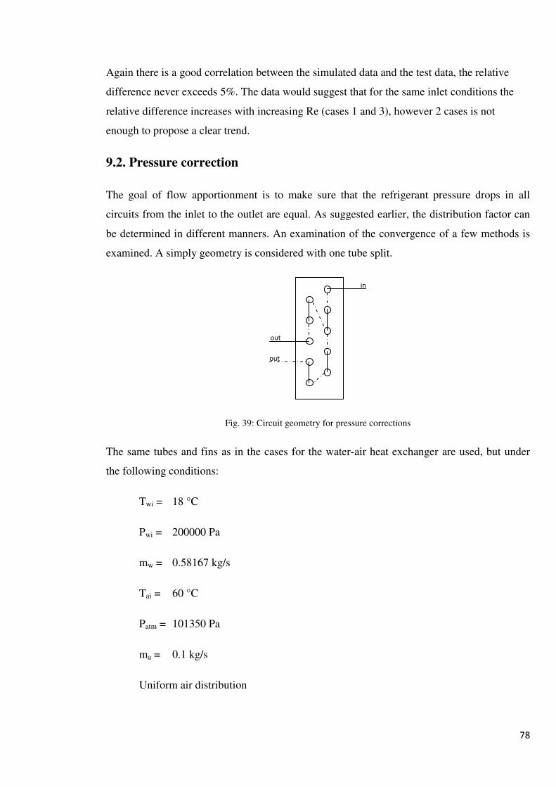
78

Again there is a good correlation between the simulated data and the test data, the relative

difference never exceeds 5%. The data would suggest that for the same inlet conditions the

relative difference increases with increasing Re (cases 1 and 3), however 2 cases is not

enough to propose a clear trend.

9.2. Pressure correction

The goal of flow apportionment is to make sure that the refrigerant pressure drops in all

circuits from the inlet to the outlet are equal. As suggested earlier, the distribution factor can

be determined in different manners. An examination of the convergence of a few methods is

examined. A simply geometry is considered with one tube split.

Fig. 39: Circuit geometry for pressure corrections

The same tubes and fins as in the cases for the water-air heat exchanger are used, but under

the following conditions:

Twi = 18 °C

Pwi = 200000 Pa

mw = 0.58167 kg/s

Tai = 60 °C

Patm = 101350 Pa

ma = 0.1 kg/s

Uniform air distribution

in

out

out

79

Case 1

∆� � ���

�� � ∆�����

�� � ∆�����

v· � �·mp.q∑ �̧ mp.q�̧»� ¿�· � v· . �

It.

nr.

#

iteration

needed

Qbefore

(W)

Qnew

(W)

m1

(kg/s)

m2

(kg/s)

Dp1

(bar)

Dp2

(bar)

1 13 0 7068.4 0.0319076 0.026259 0.0299003 0.0299003

2 7 7068.4 6987.51 0.0319096 0.0262571 0.0298345 0.0298345

3 5 6987.51 6987.4 0.0319096 0.026257 0.0298345 0.0298345

Table 9: Simulation results for quadratic pressure correction and accuracy 10-6%

1e-008 (=0,000001%) was chosen as accuracy for the pressure drop over the parallel branches

in order to clearly show the effect of the distribution correction factors.

The first estimate of the mass flow rate distribution in consecutive iterations (the larger loop

for the heat transfer) becomes closer to the final distribution, meaning that less iterations of

the smaller loop for the pressure drop correction are needed per larger loop (13 -> 7 -> 5). In

other words the last achieved values of the previous iteration are used as the first in the next.

The mass flow rates vary only very sligthly between iteration 2 and 3. A lower tolerance

would decrease the amount of iterations needed for convergence, for example 0.001 (0.1%) ,

which corresponds with ±1 Pa difference, would be more than sufficient. This data is shown

in Table 10.

80

It.

nr.

#

iteration

needed

Qbefore

(W)

Qnew

(W)

m1

(kg/s)

m2

(kg/s)

Dp1

(bar)

Dp2

(bar)

1 5 0 7068.46 0.0319011 0.0262656 0.0298905 0.0299115

2 1 7068.46 6988.87 0.0319062 0.0262605 0.0298295 0.0298422

3 1 6988.87 6985.5 0.0319093 0.0262574 0.0298323 0.0298336

Table 10: Simulation results for quadratic pressure correction and accuracy 0.1%

Case 2

∆� � ��

�� � ∆����

�� � ∆����

v· � �·m�∑ �̧ m��̧»� ¿�· � v· . �

It.

nr.

#

iteration

needed

Qbefore

(W)

Qnew

(W)

m1

(kg/s)

m2

(kg/s)

Dp1

(bar)

Dp2

(bar)

1 11 0 7068.56 0.0318989 0.0262677 0.0298872 0.0299154

2 1 7068.56 6988.77 0.0319125 0.0262542 0.0298389 0.0298313

3 1 6988.77 6985.51 0.0319088 0.0262578 0.0298316 0.0298344

Table 11: Simulation results for linear pressure correction

81

Case 3

∆� � ��j

�� � ∆����j

�� � ∆����j

v· � �·mp.jjj∑ �̧ mp.jjj�̧»� ¿�· � v· . �

It.

nr.

#

iteration

needed

Qbefore

(W)

Qnew

(W)

m1

(kg/s)

m2

(kg/s)

Dp1

(bar)

Dp2

(bar)

1 9 0 7068.51 0.0318992 0.0262675 0.0298876 0.0299149

2 1 7068.51 6988.91 0.0319033 0.0262634 0.0298251 0.0298472

3 1 6988.91 6985.54 0.0319066 0.0262601 0.0298283 0.0298382

Table 12: Simulation results for cubic pressure correction

Case 4

∆� � ��l

�� � ∆����l

�� � ∆����l

v· � �·mp.�q∑ �̧ mp.�q�̧»� ¿�· � v· .�

82

It.

nr.

#

iteration

needed

Qbefore

(W)

Qnew

(W)

m1

(kg/s)

m2

(kg/s)

Dp1

(bar)

Dp2

(bar)

1 13 0 7068.5 0.0319002 0.0262665 0.0298891 0.0299132

2 1 7068.5 6988.92 0.0319031 0.0262636 0.0298248 0.0298476

3 1 6988.92 6985.55 0.0319058 0.0262608 0.0298271 0.0298395

Table 13: Simulation results for 4th power pressure correction

In cases 2, 3 and 4 an accuracy of 0.1% was used.

From the four cases can be concluded that the pressure drop is proportional with the mass

flow rate to the power of a certain value between 2 and 3.

Although the pressure correction based on the correlation by Pierre is not applicable because

said correlations are not implemented, it is examined.

Case 5

`· � ∆�·�·�.nq

�· � �·/�

v· � 1∑ `· `̧À �p.qn��̧»� ¿�· � v· .�

It.

nr.

#

iteration

needed

Qbefore

(W)

Qnew

(W)

m1

(kg/s)

m2

(kg/s)

Dp1

(bar)

Dp2

(bar)

1 4 0 7068.44 0.0319017 0.0262649 0.0298914 0.0299104

2 1 7068.44 6988.89 0.0319049 0.0262618 0.0298275 0.0298445

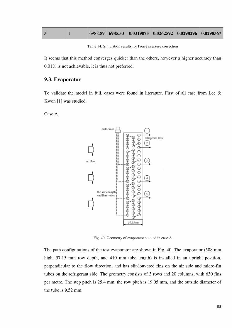
83

3 1 6988.89 6985.53 0.0319075 0.0262592 0.0298296 0.0298367

Table 14: Simulation results for Pierre pressure correction

It seems that this method converges quicker than the others, however a higher accuracy than

0.01% is not achievable, it is thus not preferred.

9.3. Evaporator

To validate the model in full, cases were found in literature. First of all case from Lee &

Kwon [1] was studied.

Case A

Fig. 40: Geometry of evaporator studied in case A

The path configurations of the test evaporator are shown in Fig. 40. The evaporator (508 mm

high, 57.15 mm row depth, and 410 mm tube length) is installed in an upright position,

perpendicular to the flow direction, and has slit-louvered fins on the air side and micro-fin

tubes on the refrigerant side. The geometry consists of 3 rows and 20 columns, with 630 fins

per metre. The step pitch is 25.4 mm, the row pitch is 19.05 mm, and the outside diameter of

the tube is 9.52 mm.

84

The volumetric flow rate of air, va, is kept constant at 18.0 m3/min, which corresponds to a

frontal velocity of 1.44 m/s. The dry and wet bulb temperatures are set at 27 and 19.5 °C,

respectively, meaning that the relative humidity is 50%. The other inlet conditions are as

follows:

R22

mri = 181.7 kg/h

Pri = 5 bar

xi = 0.20

The results:

Qtest (W) Qsim (W) RD (%)

8090 6589 -18.55

Table 15: Results Case A

This difference is unacceptable. As the simulation program works properly for the water-air

heat exchanger, the cause of this discrepancy must be found in the properties specific to

evaporators. The main differences are the presence of two phase flow and, in humid

conditions, condensation on the tubes and fins on the airside.

The correlations for two phase flow are tried and tested, so firstly the effect of condensation

will be examined. First of all it must be established if condensation takes place.

When a moist air stream is cooled at constant mixture pressure to a temperature below its dew

point temperature, some condensation of the water vapour initially present would occur. The

simulation shows us that the dew point temperatures of the cells ranges between -0.41 and

11.09 °C. 68.9% of the cell wall temperatures are beneath the respective dew point

temperature, thus when moist air streams over these cell condensation will take place. Fig. 41

shows the average wall temperature per row of tubes compared to the average dew point

temperature per row. It is apparent that in all but the last row condensation takes place.

85

Fig. 41: Condensation

A method to determine the effect of condensation on the airside is given below, this method

provides an idea of magnitude of the latent heat transfer.

From the Psychrometric Chart we can determine the humidity ratio ω of the air at the inlet. At

27 °C and 50% relative humidity, the humidity ratio is 0.095 kg water/kg air. From the Steam

Tables the value for the enthalpy of vapour can be determined: 2550.8 kJ/kg.

At the air outlet, where according to the simulation the average outlet temperature is 9.9 °C.

The mixture of air and vapour is saturated at this point, so the relative humidity is 100%.

Again, the Psychrometric Chart gives us the humidity ratio, which is 0.008 kg water/kg air.

The enthalpy for condensed liquid is 42.0 kJ/kg at these conditions.

The condensation is therefore

0.0095 0.008� BU -]:1+/BU ]9+ � 0.0015 BU -]:1+/BU ]9+

.

The energy for condensation is thus:

0.015 < 2550.8 42.0� BT/BU ]9+ � 3.763 BT/BU ]9+

The mass flow rate of dry air is

0

2

4

6

8

10

12

1 2 3

T (

°C)

Rows (-)

Tdew

Tp

86

��P*1 " S� � 0.344852 BU/8

The latent heat transfer is thus

0.344852 BU ]9+ 8⁄ < 3.763 BT BU⁄ ]9+ � 1.298 B±

Together with the sensible heat transfer this gives an estimate of the total heat transfer. The

relative difference of the sum to the test data is -2.5%.

Qtest (W) Qsens (W) Qlatent (W) Qsim (W) RD (%)

8090 6589 1298 7887 -2.51

Table 16: Results Case A + Latent Heat

The first circuit is shorter than the others, while the last is longer. It can thus be expected that,

with the same mass flow rate, the first one will offer a smaller flow resistance and the last one

a larger. Due to the flow apportionment algorithm this is adjusted. The eventual distribution is

as follows:

m1 = 0.240 mtot

m2 = 0.196 mtot

m3 = 0.196 mtot

m4 = 0.196 mtot

m5 = 0.172 mtot

The pressure drop for every circuit is represented in Fig. 42, it is apparent that the outlet

pressure is the same for the parallel circuits.

87

Fig. 42: Pressure along the coolant path

9.4. Condensation

Condensation is a difficult phenomenon to describe as both energy and mass transfer takes

place. As the water vapour present in the air comes into contact with a surface (fins and/or

tubes) that is beneath the dew point temperature for water at that pressure, water is deposited

on the surface and the latent heat is transferred. Different methods of taking the condensation

on air side into account can be found in the literature. One of the easier methods is proposed

by Domanski [2]. It uses the traditional εNTU method with some adjustments and additions.

In stead of the overall heat transfer coefficient described earlier, the following U is used:

� � £ �>;���� " �>v����LM " 1;( " �>��>;@P " 1;>1 " Á� 41 �P�> 1 OP�7¥m�

With

Ao = Air side surface

hi = Internal heat transfer coefficient

Api = Pipe inside surface

δp = Tube wall thickness

Apm = Pipe mean surface

hl = Heat transfer coefficient for condensate layer

4.91

4.92

4.93

4.94

4.95

4.96

4.97

4.98

4.99

5

5.01

p [

ba

r]

Along the refrigerant path

Circuit 1

Circuit 2

Circuit 3

Circuit 4

Circuit 5

88

Apo = Pipe outside surface

htf = Heat transfer coefficient for tube/fin contact

ho = External heat transfer coefficient

Af = Finned surface

hfgw = Latent heat of water

Á � ;P&MS� SM����� M�

The first and the fifth terms of the equation represent the refrigerant side and the air side

convection resistances. The second term is the conductive heat-transfer resistance through the

tube wall and the third term accounts for the conduction resistance through the water layer on

the fin and tube. The fourth term represents the contact resistance between the outside tube

surface and the fin collar. (1+α) in the fifth term accounts for the latent heat transfer on the

outside surface. For a dry tube α = 0 and 1/hl = 0.

With this equation the heat transfer rate can be determined. Together with the heat transfer

resistances the temperatures of the wall, the condensate layer can be found. The humidity

ratios for saturated air at wall and fin temperatures can be computed. The mass transfer from

the air to the fin and tube can then be resolved with the following equation:

ΔS � S�� SM� Â1 1%� h ;>��>N1�����ià " �S�� " SP��� Â1 1%� h ;>�PN1�����iÃ

The first term calculates the mass transfer from the air to the tube wall and the second from

the air to the fin surface. The Lewis number, Le ( = ho/(hDcpa) with hD the air side mass

transfer coefficient), is assumed 1. As the properties are unknown at the outset of the

simulation, they are initially estimated, and later the estimated values are replaced by the

values obtained in the previous iteration loop.

The outlet conditions can now be calculated:

S�> � S�� Δω

�> � �� ������� " ;P&MΔω���

89

9.5. Further Evaporator Cases

Case B

Cases in dry conditions are not readily available in literature. However, Domanski [2]

provides a break down of the simulated values into sensible and latent heat transfer. As this

computer model does not simulate the effect of condensation, the calculated heat transfer

should approach the sensible heat transfer.

The evaporator used in case B has the geometry shown in Fig. 43

Fig. 43: Geometry Case B

Table 17 contains the evaporator design data. Table 18 gives the inlet conditions

90

Item DataNumber of tube depth rows 3Number of tubes per depth row 12Tube inner diameter 9.20 mmTube outer diameter 9.91 mmTube pitch in the same depth row 25.40 mmDepth row pitch 22.00 mmCoil width (finned tube length) 914.4 mmCoil face area 0.28 m2

Fin pitch 1.81 mmFin thickness 0.14 mmFin thermal conductivity 219 W/m°CTube thermal conductivity 339 kW/m°C

Table 17: Evaporator Specification

Item DataAir inlet dry bulb temperature 26.7 °CAir inlet wet bulb temperature 19.4 °CAir volumetric flow rate 27.0 m3/minAir face velocity 96.4 m/minAir distribution uniformRefrigerant R22Refrigerant inlet pressure 645.4 kPaRefrigerant mass flow rate 212.3 kg/hRefrigerant inlet quality 0.2

Table 18: Inlet conditions

The value for the sensible heat transfer provided by Domanski is 6590 W, this model

calculated the heat transfer as 6817 W.

The relative difference is thus

�[�� �³>���[·��³>���[·� � 6817 65906590 � 3.44%

The program developed by Domanski generally under predicts the heat transfer, meaning that

this model gives better results.

91

Due to the manner in which the evaporator is simulated, it is possible to store and present

properties along the refrigerant path. For every cell all data can be written to a separate file for

later analysis.

Fig. 45: Internal heat transfer coefficient along the refrigerant path

A clear dependency between the vapour quality and the internal heat transfer coefficient is

visible as was to be expected due to the different flow patterns at different x’s.

0

0.1

0.2

0.3

0.4

0.5

0.6

0.7

0.8

0.9

Va

po

ur

qu

ali

ty x

[-]

Along refrigerant path

Circuit 1

Circuit 2

Circuit 3

Circuit 4

Circuit 5

Circuit 6

0

0.1

0.2

0.3

0.4

0.5

0.6

0.7

0.8

0

500

1000

1500

2000

2500

3000

3500

4000

4500

x [

-]

Inte

rna

l HT

C [

W/m

²K]

Along refrigerant path

Circuit 1

Circuit 2

Circuit 3

Circuit 4

Circuit 5

Circuit 6

x

Fig. 44: Vapour quality along the refrigerant path

92

Fig. 46: Refrigerant temperature along the refrigerant path

Fig. 47: Heat transfer per cell along the refrigerant path

%mtot

circuit 1

%mtot

circuit 2

%mtot

circuit 3

%mtot

circuit 4

%mtot

circuit 5

%mtot

circuit 6

16.5644 16.6418 16.6419 16.6419 16.6418 16.8682

Table 19: Refrigerant mass flow rate distribution

7.8

7.85

7.9

7.95

8

8.05

8.1

8.15

8.2

8.25

8.3

Re

frig

era

nt

tem

pe

ratu

e [

°C]

Along refrigerant path

Circuit 1

Circuit 2

Circuit 3

Circuit 4

Circuit 5

Circuit 6

0

500

1000

1500

2000

2500

3000

3500

4000

4500-16

-14

-12

-10

-8

-6

-4

-2

0

hi

[W/m

²K]

q/c

ell

[W

]

Along refrigerant path

q Circuit 1

hi Circuit 1

93

Case C

The third and final evaporator case is also from Domanski. The evaporator specifications

from Table 17 are also valid in the case, however, the geometry differs:

Fig. 48: Evaporator geometry for case C

Item DataAir inlet dry bulb temperature 26.7 °CAir inlet wet bulb temperature 19.4 °CAir volumetric flow rate 27.0 m3/minAir face velocity 96.4 m/minAir distribution uniformRefrigerant R22Refrigerant inlet pressure 646.4 kPaRefrigerant mass flow rate 211.6 kg/hRefrigerant inlet quality 0.2

Table 20: Inlet conditions

The value for the sensible heat is 6680 W, the simulations give 6912 W. The corresponds

with a relative difference of

94

�[�� �³>���[·��³>���[·� � 6912 66806680 � 3.47%

The analysed results are shown in the following graphs.

Fig. 49: Vapour quality along the refrigerant path

Fig. 50: Internal heat transfer coefficient along the refrigerant path

0

0.1

0.2

0.3

0.4

0.5

0.6

0.7

0.8

0.9

Va

po

ur

qu

ali

ty [

-]

Along refrigerant path

Circuit 1

Circuit 2

Circuit 3

Circuit 4

Circuit 5

Circuit 6

0

0.1

0.2

0.3

0.4

0.5

0.6

0.7

0.8

0.9

0

500

1000

1500

2000

2500

3000

3500

x [

-]

Va

po

ur

qu

ali

ty [

-]

Along refrigerant path

Circuit 1

Circuit 2

Circuit 3

Circuit 4

Circuit 5

Circuit 6

x

95

Fig. 51: Refrigerant temperature along the refrigerant path

Fig. 52: Refrigerant temperature along the refrigerant path

REFERENCES

[1] J. Lee and Y.C. Kwon, An improved method for analyzing a fin and tube evaporator

containing a zeotropic mixture refrigerant with air mal-distribution, International Journal of Refrigeration 26 (2003) pp. 707–720

[2] J. Lee and P.A. Domanski, Impact of air and refrigerant maldistributions on the

performance of finned-tube evaporators with R-22 and R-407C (1997)

7.9

7.95

8

8.05

8.1

8.15

8.2

8.25

8.3

8.35

Re

frig

era

nt

tem

pe

ratu

re [

°C]

Along refrigerant path

Circuit 1

Circuit 2

Circuit 3

Circuit 4

Circuit 5

Circuit 6

0

500

1000

1500

2000

2500

3000

3500-14

-12

-10

-8

-6

-4

-2

0

hi

[W/m

²K]

q/c

ell

[W

]

Along refrigerant path

q Circuit 1

hi Circuit 1

96

Chapter 10

Conclusion

A simulation model for evaporators with complex geometry was developed. This program

underestimated the heat transfer in almost all cases, meaning that the actual heat exchanger

performs better than the predictions. The simulator successfully simulated tube splitting,

parallel circuits and air maldistribution and offers huge flexibility. An apparent shortcoming

however, is the lack of a model for condensation on the airside. Some steps have been

undertaken for future implementation.

XProps insures that a great range of different refrigerants can be used without having to

change the code. It also offers a greater accuracy compared to interpolation between values in

property tables.

A trade-off can be made between accuracy and calculation time. As the model is only an

representation of reality, relaxing the tolerances does not necessarily mean that the results will

be further from the truth, a shorter calculation time thus might be preferred.

97

APPENDIX A

98

99

100