OnthePerformanceEvaluationofDifferent MeasuresofAssociation ·...
24
Revista Colombiana de Estadística Junio 2014, volumen 37, no. 1, pp. 1 a 24 On the Performance Evaluation of Different Measures of Association Evaluación de diferentes medidas de asociación Muhammad Riaz 1, a , Shahzad Munir 2, b , Zahid Asghar 2, c 1 Department of Mathematics and Statistics, King Fahad University of Petroleum and Minerals, Dhahran, Saudi Arabia 2 Department of Statistics, Quaid-i-Azam University, Islamabad, Pakistan Abstract In this article our objective is to evaluate the performance of different measures of associations for hypothesis testing purposes. We have consid- ered different measures of association (including some commonly used) in this study, one of which is parametric and others are non-parametric including three proposed modifications. Performance of these tests are compared un- der different symmetric, skewed and contaminated probability distributions that include Normal, Cauchy, Uniform, Laplace, Lognormal, Exponential, Weibull, Gamma, t, Chi-square, Half Normal, Mixed Weibull and Mixed Normal. Performances of these tests are measured in terms of power. We have suggested appropriate tests which may perform better under different situations based on their efficiency grading(s). It is expected that researchers will find these results useful in decision making. Key words : Measures of association, Non-Normality, Non-Parametric meth- ods, Normality, Parametric methods, Power. Resumen En este articulo el objetivo es evaluar el desempeño de diferentes medi- das de asociación para pruebas de hipótesis. Se consideran diferentes medi- das, algunas paramétricas y otras no paramétricas, así como tres modifica- ciones propuestas por los autores. El desempeño de estas pruebas se evalúa considerando distribuciones simétricas, sesgadas y contaminadas incluyendo la distribución normal, Cauchy, uniforme, Laplace, lognormal, exponencial, Weibull, Gamma, t, Chi-cuadrado, medio normal, Weibull mezclada y nor- mal mezclada. El desempeño se evalúa en términos de la potencia de los tests. Se sugieren tests apropiados que tienen un mejor desempeño bajo a Professor. E-mail: [email protected] b Professor. E-mail: [email protected] c Professor. E-mail: [email protected] 1
-
Upload
nguyenkhanh -
Category
Documents
-
view
219 -
download
0
Transcript of OnthePerformanceEvaluationofDifferent MeasuresofAssociation ·...

Revista Colombiana de EstadísticaJunio 2014, volumen 37, no. 1, pp. 1 a 24
On the Performance Evaluation of DifferentMeasures of Association
Evaluación de diferentes medidas de asociación
Muhammad Riaz1,a, Shahzad Munir2,b, Zahid Asghar2,c
1Department of Mathematics and Statistics, King Fahad University of Petroleumand Minerals, Dhahran, Saudi Arabia
2Department of Statistics, Quaid-i-Azam University, Islamabad, Pakistan
Abstract
In this article our objective is to evaluate the performance of differentmeasures of associations for hypothesis testing purposes. We have consid-ered different measures of association (including some commonly used) in thisstudy, one of which is parametric and others are non-parametric includingthree proposed modifications. Performance of these tests are compared un-der different symmetric, skewed and contaminated probability distributionsthat include Normal, Cauchy, Uniform, Laplace, Lognormal, Exponential,Weibull, Gamma, t, Chi-square, Half Normal, Mixed Weibull and MixedNormal. Performances of these tests are measured in terms of power. Wehave suggested appropriate tests which may perform better under differentsituations based on their efficiency grading(s). It is expected that researcherswill find these results useful in decision making.
Key words: Measures of association, Non-Normality, Non-Parametric meth-ods, Normality, Parametric methods, Power.
Resumen
En este articulo el objetivo es evaluar el desempeño de diferentes medi-das de asociación para pruebas de hipótesis. Se consideran diferentes medi-das, algunas paramétricas y otras no paramétricas, así como tres modifica-ciones propuestas por los autores. El desempeño de estas pruebas se evalúaconsiderando distribuciones simétricas, sesgadas y contaminadas incluyendola distribución normal, Cauchy, uniforme, Laplace, lognormal, exponencial,Weibull, Gamma, t, Chi-cuadrado, medio normal, Weibull mezclada y nor-mal mezclada. El desempeño se evalúa en términos de la potencia de lostests. Se sugieren tests apropiados que tienen un mejor desempeño bajo
aProfessor. E-mail: [email protected]. E-mail: [email protected]. E-mail: [email protected]
1

2 Muhammad Riaz, Shahzad Munir & Zahid Asghar
diferentes niveles de eficiencia. Se espera que los investigadores encuentrenestos resultados útiles en la toma de decisiones.
Palabras clave: medidas de asociación, no normalidad, métodos no paramétri-cos, métodos paramétricos, potencia.
1. Introduction
It is indispensable to apply statistical tests in almost all the observational andexperimental studies in the fields of agriculture, business, biology, engineering etc.These tests help the researchers to reach at the valid conclusions of their studies.There are number of statistical testing methods in literature meant for differentobjectives, for example some are designed for association dispersion, proportionand location parameter(s). Each method has a specific objective with a particularframe of application. When more than one method qualifies for a given situation,then choosing the most suitable one is of great importance and needs extremecaution. This mostly depends on the properties of the competing methods forthat particular situation. From a statistical viewpoint, power is considered as anappropriate criterion of selecting the finest method out of many possible ones. Inthis paper our concern is with the methods developed for measuring and testing theassociation between the variables of interest defined on a some population(s). Forthe sake of simplicity we restrict ourselves with the environment of two correlatedvariables i.e. the case of bivariate population(s).
The general procedural framework can be laid down as follows: Let we have twocorrelated random variables of interest X and Y defined on a bivariate populationwith their association parameter denoted by ρ. To test the hypothesis H0 : ρ = 0(i.e. no association) vs. H1 : ρ 6= 0, we have a number of statistical methodsavailable depending upon the assumption(s) regarding the parent distribution(s).In parametric environment the usual Pearson correlation coefficient is the mostfrequent choice (cf. Daniel 1990) while in non parametric environment we havemany options. To refer the most common of these: Spearman rank correlationcoefficient introduced by Spearman (1904); Kendall’s tau coefficient proposed byKendall (1938); a modified form of Spearman rank correlation coefficient whichis known as modified rank correlation coefficient proposed by Zimmerman (1994);three Gini’s coefficients based measures of association given by Yitzhaki (2003)(two of which are asymmetrical measures and one is symmetrical). We shall re-fer all the aforementioned measures with the help of notations given in Table 1throughout this chapter.
This study is planned to investigate the performance of different measures ofassociation under different distributional environments. The association measurescovered in the study include some existing and some proposed modifications andperformance is measured in terms of power under different probability models.The organization of the rest of the article is as: Section 2 provides descriptionof different existing measures of association; Section 3 proposes some modifiedmeasures of association; Section 4 deals with performance evaluations of thesemeasures; Section 5 offers a comparative analysis of these measures; Section 6
Revista Colombiana de Estadística 37 (2014) 1–24

On the Performance Evaluation of Different Measures of Association 3
includes an illustrative example; Section 7 provides summary and conclusions ofthe study.
Table 1: Notations.rP The usual Pearson Product Moment Correlation Coefficient (cf. Daniel 1990)
proposed by Karl PearsonrS Spearman Rank Correlation Coefficient (cf. Spearman 1904)rM Modified Rank Correlation Coefficient (cf. Zimmerman 1994)rg1 Gini Correlation Coefficient between X and Y (asymmetric) (cf. Yitzhaki 2003)rg2 Gini Correlation Coefficient between Y and X (asymmetric) (cf. Yitzhaki 2003)rg3 Gini Correlation Coefficient between X and Y or between Y and X (symmetric)
(cf. Yitzhaki 2003)τ Kendall’s Tau (cf. Kendall 1938)
2. Measures of Association
In order to define and describe the above mentioned measures, let we havetwo dependent random samples in the form of pairs (x1, y1), (x2, y2), . . . , (xn, yn)drawn from a bivariate population (with the association parameter ρ) under all theassumptions needed for a valid application of all the association measures underconsideration. The description of the above mentioned measures along with theirmain features and their respective test statistics are provided below:
Pearson Product Moment Correlation Coefficient (rP ): It is a measureof the relative strength of the linear relationship between two numerical variablesof interest X and Y . The mathematical definition for this measure (denoted byrP ) is given as:
rP =cov(X,Y )
SD(X)SD(Y )(1)
where cov(X,Y ) refers to the covariance between X and Y ; SD(X) and SD(Y )are the standard deviations of X and Y respectively.
The value of rP ranges from −1 to +1 implying perfect negative and positivecorrelation respectively. A value of zero for rP means that there is no linearcorrelation between X and Y . It requires the data on at least interval scale ofmeasurement. It is a symmetric measure that is invariant of the changes in locationand scale. Geometrically it is defined as the cosine of the angle between thetwo regression lines (Y on X and X on Y ). It is not robust to the presence ofoutliers in the data. To test the statistical significance of rP we may use theusual t-test (under normality) and even under non-normality t-test may be a safeapproximation.
Spearman Rank Correlation Coefficient (rS): It is defined as the Pearsonproduct moment correlation coefficient between the ranked information of X andY rather than their raw scores. The mathematical definition for this measure(denoted by rS) is given as:
rS = 1−6∑n
i=1D2i
n(n2 − 1)(2)
Revista Colombiana de Estadística 37 (2014) 1–24

4 Muhammad Riaz, Shahzad Munir & Zahid Asghar
where n is the sample size;∑n
i=1D2i is the sum of the squares of the differences
between the ranks of two samples after ranking the samples individually. It is anon-parametric measure that lies between −1 to +1 (both inclusive) referring toperfect negative and positive correlations respectively. The sign of rS indicatesthe direction of relationship between the actual variables of interest. A value ofzero for rS means that there is no interdependency between the original variables.It requires the data on at least ordinal scale. Using normal approximation, thestatistical significance of rS may tested using the usual t-test. Modified Rank Cor-relation Coefficient (rM ): It is a modified version of Spearman rank correlationcoefficient based on transformations of X and Y into standard scores and then us-ing the concept of ranking.The mathematical definition for this measure (denotedby rM ) is given as:
rM = 1−6∑n
i=1 d2i
n(n2 − 1)(3)
where d is the difference between the ranks assigned transforming the values of Xand Y separately into standard scores, assigning the ranks to standard scores col-lectively and then make separate groups of the ranks according to their respectiverandom samples. Now defines the difference between the ranks and
∑ni=1 d
2i in (3)
is the sum of the squares of the differences between the ranks.It is also a non-parametric measure that may take zero value for no corre-
lation, positive value and negative values for negative and positive correlationsrespectively, as in the above case. A value of −1 refers to the perfect correlationsamong the variables of interest.
Gini Correlation Coefficient (Asymmetric and Symmetric): Thesecorrelation measures are based on the covariance measures between the originalvariables X and Y and their cumulative distribution functions FX(X) and FY (Y ).We consider here three measures of association based on Gini’s coefficients (twoof which are asymmetrical measures and one is symmetrical). These measures ofassociation, denoted by rg1, rg2 and rg3, are defined as:
rg1 =cov(X,FY (Y ))
cov(X,FX(X))(4)
rg2 =cov(Y, FX(X))
cov(Y, FY (Y ))(5)
rg3 =GXrg1 +GY rg2
GX +GY(6)
where cov(X,FY (Y )) is the covariance between X and cumulative distributionfunction of Y ; cov(Y, FX(X)) is the covariance between X and its cumulativedistribution function; cov(Y, FX(X)) is the covariance between Y and cumulativedistribution function of X; cov(Y, FY (Y )) is the covariance between Y and its cu-mulative distribution function; GX = 4cov(X,FX(X)) and GY = 4cov(Y, FY (Y )).
In the above mentioned measures given in (4)-(6), rg1 and rg2 are the asymmet-ric Gini correlation coefficients while rg3 is the symmetric Gini correlation coeffi-cient. Here are some properties of Gini correlation coefficients (cf. Yitzhaki 2003):The Gini coefficient is bounded, such that +1 ≥ rgjs ≥ −1(j, s = X,Y ). If X
Revista Colombiana de Estadística 37 (2014) 1–24

On the Performance Evaluation of Different Measures of Association 5
and Y are independent then; rg1 = rg2 = 0; rg2 is not sensitive to a monotonictransformation of Y . In general, rgjs need not be equal to rgsj and they may evenhave different signs. If the random variables Zj and Zs are exchangeable up to alinear transformation, then rgjs = rgsj .
Kendall’s Tau (τ): It is a measure of the association between two measuredvariables of interests X and Y . It is defined as the rank correlation based on thesimilarity orderings of the data with ranked setup. The mathematical definitionfor this measure (denoted by τ) is given as:
τ =S
n(n−1)2
(7)
where n is the size of sample and S is defined as the difference between the numberof pairs in natural and reverse natural orders. We may define S more precisely asarranging the observations (Xi, Yi) (where i = 1, 2, . . . , n) in a column accordingto the magnitude of the X ′s, with the smallest X first, the second smallest secondand so on. Then we say that the X ′s are in natural order. Now in equation (7),S is equal to P − Q, where P is the number of pairs in natural order and Q isnumber of pairs in reverse order of random variable Y .
This measure is non-parametric being free from the parent distribution. It takesvalues between +1 and −1 (both inclusive). A value equal to zero indicates nocorrelation, +1 means perfect positive and −1 means perfect negative correlation.It requires the data on at least ordinal scale. Under independence its mean is zeroand variance 2(2n+ 5)/9n(n− 1).
3. Proposed Modifications
Taking the motivations from the aforementioned measures as given in equation(1)-(7) we suggest here three modified proposals to measure association. In orderto define rM in equation (3), Zimmerman (1994) used mean as an estimate ofthe location parameter to convert the variables into standard scores. Mean as ameasure of location is able to produce reliable results when data is normal or atleast symmetrical because it is highly affected by the presence of outliers as wellas due to the departure from normality. It means that the sample mean is not arobust estimator and hence cannot give trustworthy outcomes. To overcome thisproblem, we may use median and trimmed mean as alternative measures. Thereason being that in case of non-normal distributions and/or when outliers arepresent in the data median and trimmed mean exhibit robust behavior and hencethe results based on them are expected to become more reliable than mean.
Based on the above discussion we now suggest here three modifications/propo-sals to measure the association. These three proposals are modified forms ofSpearman rank correlation coefficient, namely i) trimmed mean rank correlationby using standard deviation about trimmed mean; ii) median rank correlationby using standard deviation about median; iii) median rank correlation by usingmean deviation about median. These three proposals are based on Spearman
Revista Colombiana de Estadística 37 (2014) 1–24

6 Muhammad Riaz, Shahzad Munir & Zahid Asghar
rank correlation coefficient in which we shall transform the variables into standardscores (like in Zimmerman (1994) using the measures given in (i)-(iii) above. Weshall refer the three proposed modifications with the help of notations given inTable 2 throughout this chapter.
Table 2: Notations Table for the Proposed Modifications.rT Trimmed Rank Correlation CoefficientrMM Median Rank Correlation Coefficient by using Mean Deviation about MedianrMS Median Rank Correlation Coefficient by using Standard Deviation about Median
Keeping intact the descriptions of equation (1)-(7) we now provide the expla-nation of the three proposed modified measures. Before that we defined here fewterms used in the definitions of rT , rMM and rMS . These terms include Stan-dard Deviation by using Trimmed Mean (denoted by SD1(X) and SD1(Y ) for Xand Y respectively), Mean Deviation about Median (denoted by MDM(X) andMDM(Y ) for X and Y respectively) and Standard Deviation by using Median(denoted by SD2(X) and SD2(Y ) for X and Y respectively). These terms aredefined as under:
SD1(X) =
√∑ni=1(Xi − Xt)2
n− 1and SD1(Y ) =
√∑ni=1(Yi − Yt)2n− 1
(8)
In equation (8), Xt and Y t are the trimmed means of X and Y respectively.
MDM(X) =
∑ni=1 |Xi − X|
nand MDM(Y ) =
∑ni=1 |Yi − Y |
n(9)
In equation (9), X and Y are the medians of X and Y respectively.
SD2(X) =
√∑ni=1(Xi − Xt)2
n− 1and SD2(Y ) =
√∑ni=1(Yi − Yt)2n− 1
(10)
In equation (10), all the terms are as defined earlier.Based on the above definitions we are now able to define rT , rM and rMS as
under:
rT = 1−6∑n
i=1 d2i,T
n(n2 − 1)(11)
For equation (11); first we separately transform the values of random variables Xand Y into standard scores by using their respective trimmed means and standarddeviation about trimmed means of their respective random sample from (X,Y ),assign the ranks to standard scores collectively and then separate the ranks ac-cording to their random samples. Now in equation (11),
∑ni=1 d
2i,T is the sum of
the squares of the differences between the ranks. It is to be mentioned that wehave trimmed 2 values from each sample, so the percentages of trimming in ourcomputations are 33%, 25%, 20%, 17%, 13%, 10% and 7% of samples 6, 8, 10, 12,16, 20 and 30 respectively.
rM = 1−6∑n
i=1 d2i,MS
n(n2 − 1)(12)
Revista Colombiana de Estadística 37 (2014) 1–24
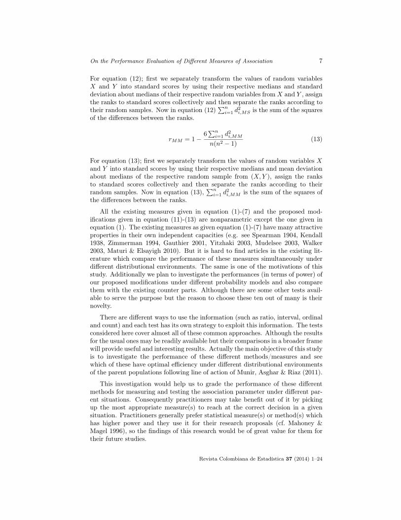
On the Performance Evaluation of Different Measures of Association 7
For equation (12); first we separately transform the values of random variablesX and Y into standard scores by using their respective medians and standarddeviation about medians of their respective random variables fromX and Y , assignthe ranks to standard scores collectively and then separate the ranks according totheir random samples. Now in equation (12)
∑ni=1 d
2i,MS is the sum of the squares
of the differences between the ranks.
rMM = 1−6∑n
i=1 d2i,MM
n(n2 − 1)(13)
For equation (13); first we separately transform the values of random variables Xand Y into standard scores by using their respective medians and mean deviationabout medians of the respective random sample from (X,Y ), assign the ranksto standard scores collectively and then separate the ranks according to theirrandom samples. Now in equation (13),
∑ni=1 d
2i,MM is the sum of the squares of
the differences between the ranks.
All the existing measures given in equation (1)-(7) and the proposed mod-ifications given in equation (11)-(13) are nonparametric except the one given inequation (1). The existing measures as given equation (1)-(7) have many attractiveproperties in their own independent capacities (e.g. see Spearman 1904, Kendall1938, Zimmerman 1994, Gauthier 2001, Yitzhaki 2003, Mudelsee 2003, Walker2003, Maturi & Elsayigh 2010). But it is hard to find articles in the existing lit-erature which compare the performance of these measures simultaneously underdifferent distributional environments. The same is one of the motivations of thisstudy. Additionally we plan to investigate the performances (in terms of power) ofour proposed modifications under different probability models and also comparethem with the existing counter parts. Although there are some other tests avail-able to serve the purpose but the reason to choose these ten out of many is theirnovelty.
There are different ways to use the information (such as ratio, interval, ordinaland count) and each test has its own strategy to exploit this information. The testsconsidered here cover almost all of these common approaches. Although the resultsfor the usual ones may be readily available but their comparisons in a broader framewill provide useful and interesting results. Actually the main objective of this studyis to investigate the performance of these different methods/measures and seewhich of these have optimal efficiency under different distributional environmentsof the parent populations following line of action of Munir, Asghar & Riaz (2011).
This investigation would help us to grade the performance of these differentmethods for measuring and testing the association parameter under different par-ent situations. Consequently practitioners may take benefit out of it by pickingup the most appropriate measure(s) to reach at the correct decision in a givensituation. Practitioners generally prefer statistical measure(s) or method(s) whichhas higher power and they use it for their research proposals (cf. Mahoney &Magel 1996), so the findings of this research would be of great value for them fortheir future studies.
Revista Colombiana de Estadística 37 (2014) 1–24
8 Muhammad Riaz, Shahzad Munir & Zahid Asghar
4. Performance Evaluations
Power is an important measure for the performance of a testing procedure.It is the probability of rejecting H0 when it is false and it is the probabilitythat a statistical measure(s)/procedure(s) will lead to a correct decision. In thissection we intend to evaluate the power of the ten association measures underconsideration in this study and find out which of them have relatively higherpower(s) than the others under different parent situations. To calculate the powerof different methods of measuring and testing the association under study we havefollowed the following procedure for power evaluations.
Let X and Y be the two correlated random variables referring to the two interdependent characteristics of interest from where we have a random sample of npairs in the form of (x1, y1), (x2, y2),. . . ,(xn, yn) from a bivariate population. Toget the desire level of correlation between X and Y the steps are listed as:
• Let X and Y be independent random variables and Y be a transformedrandom variable defined as: Y = a(X) + b(W );
• The correlation between X and Y is given as: rXY = a√a2+b2
, where a andb are unknown constants;
• The expression for a in the form of b and rXY may be written as a = b(rXY )√1−r2XY
,
• If b=1 then we have: a = rXY√1−r2XY
, and by putting the desire level of corre-
lation in this equation we get the value of a;
• For the above mentioned values of a and b we can now obtain the variablesX and Y having our desired correlation level.
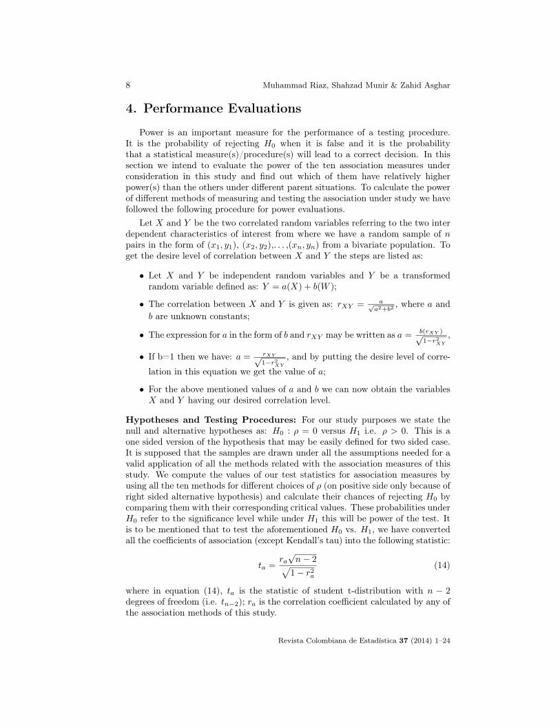
Hypotheses and Testing Procedures: For our study purposes we state thenull and alternative hypotheses as: H0 : ρ = 0 versus H1 i.e. ρ > 0. This is aone sided version of the hypothesis that may be easily defined for two sided case.It is supposed that the samples are drawn under all the assumptions needed for avalid application of all the methods related with the association measures of thisstudy. We compute the values of our test statistics for association measures byusing all the ten methods for different choices of ρ (on positive side only because ofright sided alternative hypothesis) and calculate their chances of rejecting H0 bycomparing them with their corresponding critical values. These probabilities underH0 refer to the significance level while under H1 this will be power of the test. Itis to be mentioned that to test the aforementioned H0 vs. H1, we have convertedall the coefficients of association (except Kendall’s tau) into the following statistic:
ta =ra√n− 2√
1− r2a(14)
where in equation (14), ta is the statistic of student t-distribution with n − 2degrees of freedom (i.e. tn−2); ra is the correlation coefficient calculated by any ofthe association methods of this study.
Revista Colombiana de Estadística 37 (2014) 1–24
On the Performance Evaluation of Different Measures of Association 9
Distributional Models: In order to cover the commonly used practical mod-els of parent distributions, we have considered (in bivariate setup) Normal, Uni-form, Laplace, Lognormal, Exponential, Weibull, Gamma, Half Normal, MixedWeibull, and Mixed Normal distributions as some representative parent distribu-tions for our study. We also include Gamma, Exponential and Weibull distribu-tions with outliers (contamination) in our study. For the choices of the distribu-tions of X and Y , we have the following particular parameter selections to createbivariate environments: N(0, 1) for Normal; U(0, 1) for Uniform; L(0.5, 3) forLaplace; LN(0, 1) for Lognormal; Exp(0.5) for Exponential; W (1, 2) for Weibull;G(1, 2) for Gamma; HN(0, 1) for Half Normal;W (0.5, 3) with probability 0.95 andW (1, 2) with probability 0.05 for Mixed Weibull; N(0, 1) with probability 0.95 andN(0, 400) with probability 0.05 for Mixed Normal; G(0.5, 3) with 5% outliers fromG(4, 10) for contaminated Gamma; W (1, 2) with 5% outliers from W (50, 100) forcontaminated Wiebull; exp(0.5) with 5% outliers from exp(4) for contaminatedExponential.
Computational Details of Experimentation: We have computed powersof the ten methods of measuring and testing the association by fixing the sig-nificance level at α using a simulation code developed in MINITAB. The criticalvalues at a given α are obtained from the table of tn−2 for all the measures givenin Equation ((1)-(7) and (11)-(13)) and their corresponding test statistics givenin Equation (14), except for Kendall’s coefficient given in Equation (7). For theKendall’s tau coefficient (τ) we have used the true critical values as given in Daniel(1990). The reason being that for all other cases the approximation given in Equa-tion (14) is able to work fairly good but for the Kendall’s tau coefficient it is notthe case (as we here observed in our computations). The change in shape of theparent distribution demands an adjustment in the corresponding critical values.This we have done by our simulation algorithm for these ten methods to achievethe desired value of α. For different choices of ρ = 0, 0.25, 0.5 and 0.75 powers areobtained with the help of our simulation code in MINITAB at α significance level.
We have considered thirteen representative bivariate environments mentionedabove for n = 6, 8, 10, 12, 16, 20, 30 at varying values of α. For these choices of n, αwe have run our MINITAB simulation code (developed for the ten methods underinvestigation here) 10,000 times for power computations. The resulting powervalues are given in the tables given in Appendix for all the thirteen probabilitydistributions and the ten methods under study for some selective choices from theabove mentioned values of n at α = 0.05. For the sake of brevity we omit theresults at other choices of α like 0.01 and 0.005.
5. Comparative Analysis
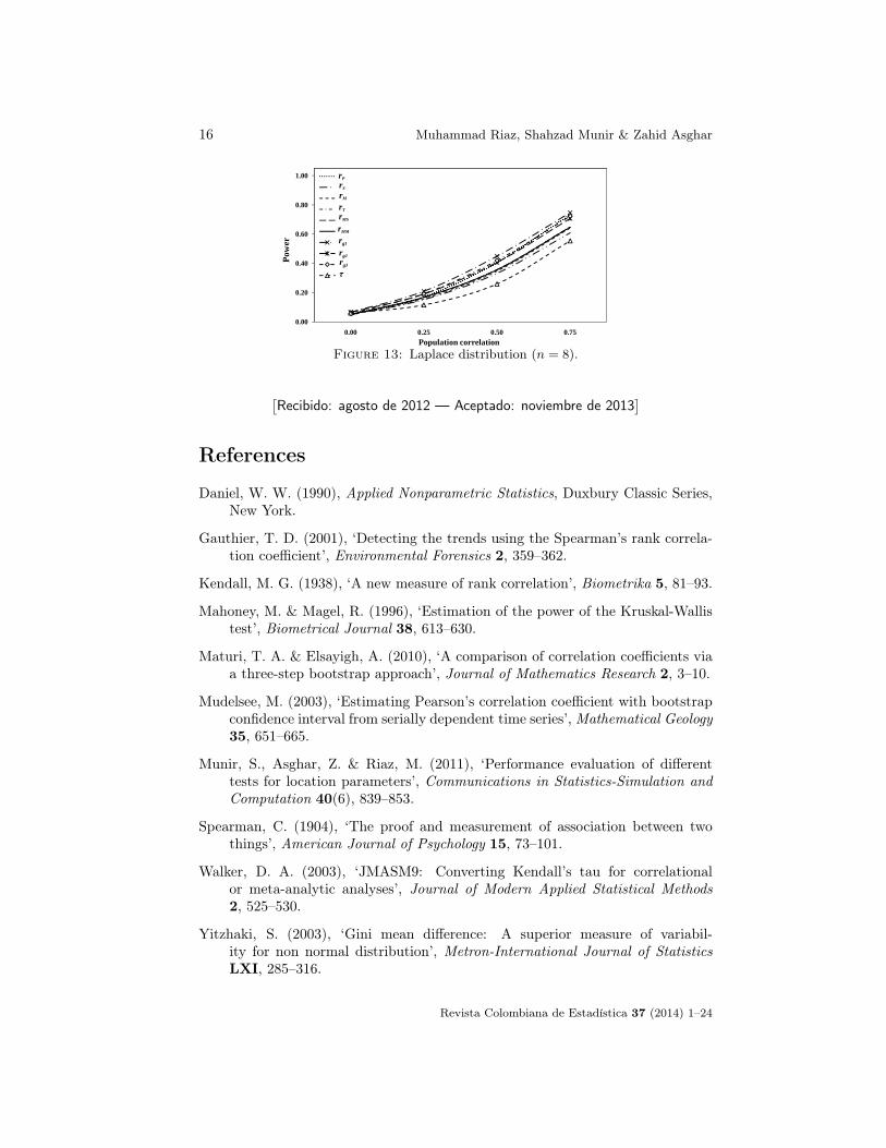
This section presents a comparative analysis of the existing and proposed as-sociation measures. For ease in discussion and comparisons, the power valuesmentioned above are also displayed graphically in the form of power curves for allthe aforementioned thirteen probability distributions by taking particular samplesizes and ten methods of association for some selective cases. These graphs are
Revista Colombiana de Estadística 37 (2014) 1–24
10 Muhammad Riaz, Shahzad Munir & Zahid Asghar
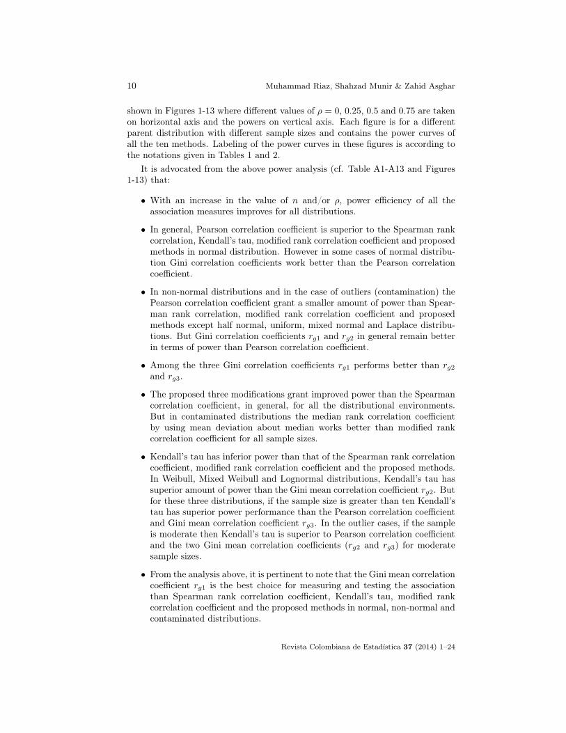
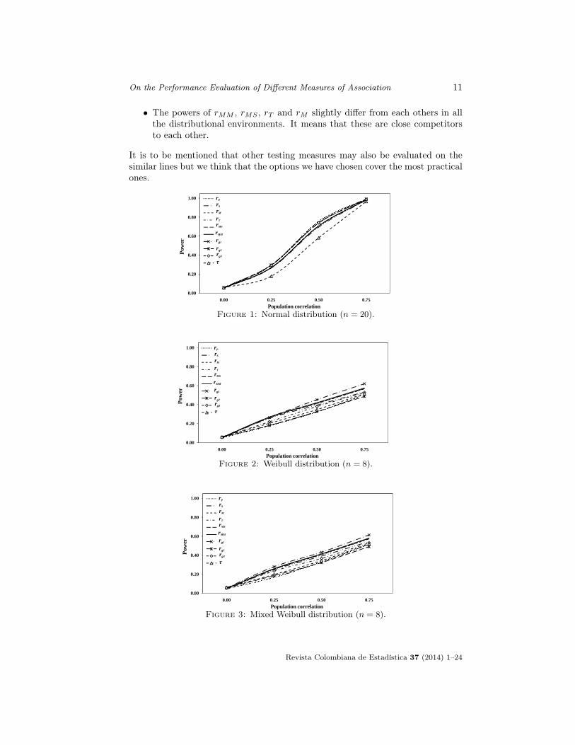
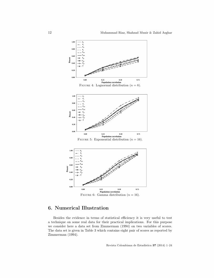
shown in Figures 1-13 where different values of ρ = 0, 0.25, 0.5 and 0.75 are takenon horizontal axis and the powers on vertical axis. Each figure is for a differentparent distribution with different sample sizes and contains the power curves ofall the ten methods. Labeling of the power curves in these figures is according tothe notations given in Tables 1 and 2.
It is advocated from the above power analysis (cf. Table A1-A13 and Figures1-13) that:
• With an increase in the value of n and/or ρ, power efficiency of all theassociation measures improves for all distributions.
• In general, Pearson correlation coefficient is superior to the Spearman rankcorrelation, Kendall’s tau, modified rank correlation coefficient and proposedmethods in normal distribution. However in some cases of normal distribu-tion Gini correlation coefficients work better than the Pearson correlationcoefficient.
• In non-normal distributions and in the case of outliers (contamination) thePearson correlation coefficient grant a smaller amount of power than Spear-man rank correlation, modified rank correlation coefficient and proposedmethods except half normal, uniform, mixed normal and Laplace distribu-tions. But Gini correlation coefficients rg1 and rg2 in general remain betterin terms of power than Pearson correlation coefficient.
• Among the three Gini correlation coefficients rg1 performs better than rg2and rg3.
• The proposed three modifications grant improved power than the Spearmancorrelation coefficient, in general, for all the distributional environments.But in contaminated distributions the median rank correlation coefficientby using mean deviation about median works better than modified rankcorrelation coefficient for all sample sizes.
• Kendall’s tau has inferior power than that of the Spearman rank correlationcoefficient, modified rank correlation coefficient and the proposed methods.In Weibull, Mixed Weibull and Lognormal distributions, Kendall’s tau hassuperior amount of power than the Gini mean correlation coefficient rg2. Butfor these three distributions, if the sample size is greater than ten Kendall’stau has superior power performance than the Pearson correlation coefficientand Gini mean correlation coefficient rg3. In the outlier cases, if the sampleis moderate then Kendall’s tau is superior to Pearson correlation coefficientand the two Gini mean correlation coefficients (rg2 and rg3) for moderatesample sizes.
• From the analysis above, it is pertinent to note that the Gini mean correlationcoefficient rg1 is the best choice for measuring and testing the associationthan Spearman rank correlation coefficient, Kendall’s tau, modified rankcorrelation coefficient and the proposed methods in normal, non-normal andcontaminated distributions.
Revista Colombiana de Estadística 37 (2014) 1–24
On the Performance Evaluation of Different Measures of Association 11
• The powers of rMM , rMS , rT and rM slightly differ from each others in allthe distributional environments. It means that these are close competitorsto each other.
It is to be mentioned that other testing measures may also be evaluated on thesimilar lines but we think that the options we have chosen cover the most practicalones.
0.80
1.00 rP
rM
rS
rT
rMS
rMM
0.00
0.20
0.40
0.60
0.00 0.25 0.50 0.75
Pow
er
Population correlation
rMM
rg2
rg1
rg3
τ
Figure 1: Normal distribution (n = 20).
0.80
1.00 rP
rM
rS
rT
rMS
rMM
Wiebull distribution (n=8)
0.00
0.20
0.40
0.60
0.00 0.25 0.50 0.75
Pow
er
Population correlation
rMM
rg2
rg1
rg3
τ
Figure 2: Weibull distribution (n = 8).
0.80
1.00 rP
rM
rS
rT
rMS
rMM
Mixed Wiebull distribution (n=8)
0.00
0.20
0.40
0.60
0.00 0.25 0.50 0.75
Pow
er
Population correlation
rMM
rg2
rg1
rg3
τ
Figure 3: Mixed Weibull distribution (n = 8).
Revista Colombiana de Estadística 37 (2014) 1–24
12 Muhammad Riaz, Shahzad Munir & Zahid Asghar
0.80
1.00 rP
rM
rS
rT
rMS
rMM
Lognormal distribution (n=8)
0.00
0.20
0.40
0.60
0.00 0.25 0.50 0.75
Pow
er
Population correlation
rMM
rg2
rg1
rg3
τ
Figure 4: Lognormal distribution (n = 8).
0.80
1.00 rP
rM
rS
rT
rMS
rMM
Exponential distribution (n=16)
0.00
0.20
0.40
0.60
0.00 0.25 0.50 0.75
Pow
er
Population correlation
rMM
rg2
rg1
rg3
τ
Figure 5: Exponential distribution (n = 16).
0.80
1.00 rP
rM
rS
rT
rMS
rMM
Gamma distribution (n=16)
0.00
0.20
0.40
0.60
0.00 0.25 0.50 0.75
Pow
er
Population correlation
rMM
rg2
rg1
rg3
τ
Figure 6: Gamma distribution (n = 16).
6. Numerical Illustration
Besides the evidence in terms of statistical efficiency it is very useful to testa technique on some real data for their practical implications. For this purposewe consider here a data set from Zimmerman (1994) on two variables of scores.The data set is given in Table 3 which contains eight pair of scores as reported byZimmerman (1994).
Revista Colombiana de Estadística 37 (2014) 1–24
On the Performance Evaluation of Different Measures of Association 13
Table 3: Eight pairs of Scores.Pair#
1 2 3 4 5 6 7 8Scores X 3.02 15.7 9.88 20.53 17.1 18.15 17.52 1.7
Y 43.02 52.84 54.25 57.99 52.35 47.4 55.37 49.52
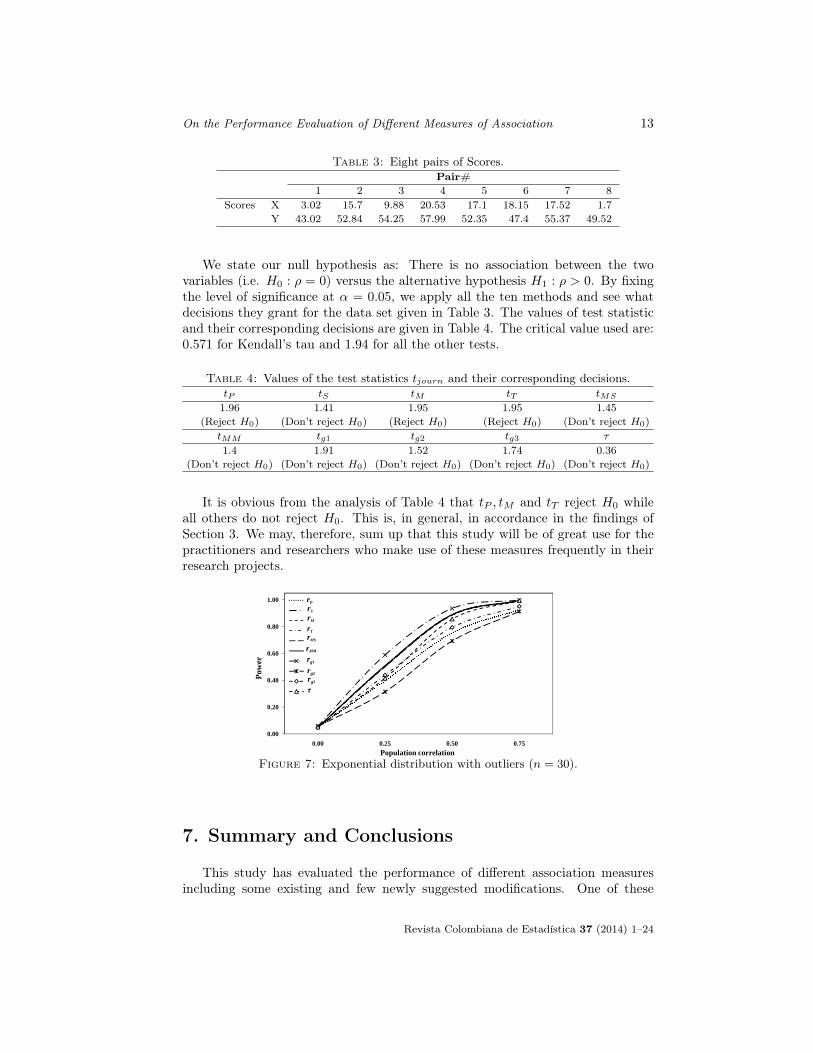
We state our null hypothesis as: There is no association between the twovariables (i.e. H0 : ρ = 0) versus the alternative hypothesis H1 : ρ > 0. By fixingthe level of significance at α = 0.05, we apply all the ten methods and see whatdecisions they grant for the data set given in Table 3. The values of test statisticand their corresponding decisions are given in Table 4. The critical value used are:0.571 for Kendall’s tau and 1.94 for all the other tests.
Table 4: Values of the test statistics tjourn and their corresponding decisions.tP tS tM tT tMS
1.96 1.41 1.95 1.95 1.45(Reject H0) (Don’t reject H0) (Reject H0) (Reject H0) (Don’t reject H0)
tMM tg1 tg2 tg3 τ
1.4 1.91 1.52 1.74 0.36(Don’t reject H0) (Don’t reject H0) (Don’t reject H0) (Don’t reject H0) (Don’t reject H0)
It is obvious from the analysis of Table 4 that tP , tM and tT reject H0 whileall others do not reject H0. This is, in general, in accordance in the findings ofSection 3. We may, therefore, sum up that this study will be of great use for thepractitioners and researchers who make use of these measures frequently in theirresearch projects.
0.80
1.00 rP
rM
rS
rT
rMS
rMM
Exponential distribution with outliers (n=30)
0.00
0.20
0.40
0.60
0.00 0.25 0.50 0.75
Pow
er
Population correlation
rMM
rg2
rg1
rg3
τ
Figure 7: Exponential distribution with outliers (n = 30).
7. Summary and Conclusions
This study has evaluated the performance of different association measuresincluding some existing and few newly suggested modifications. One of these
Revista Colombiana de Estadística 37 (2014) 1–24

14 Muhammad Riaz, Shahzad Munir & Zahid Asghar
measures is parametric and the others non-parametric ones. Performance evalua-tions (in terms of power) and comparisons are carried out under different symmet-ric, skewed and contaminated probability distributions including Normal, Cauchy,Uniform, Laplace, Lognormal, Exponential, Weibull, Gamma, t, Chi-square, HalfNormal, Mixed Weibull and Mixed Normal.
Power evaluations of this study revealed that in normal distribution the Pear-son correlation coefficient is the best choice to measure association. Further wehave observed that the Pearson correlation coefficient and Gini’s correlation coef-ficients (rg2 and rg3) have superior power performances than the Spearman rankcorrelation, The modified rank correlation and the proposed correlation coefficientsfor symmetrical and low peaked distributions. But in non-symmetrical and highpeaked distributions the Spearman rank correlation, modified rank correlation andthe proposed correlation coefficients worked with supreme power than the Pearsoncorrelation coefficient and the two Gini’s correlation coefficients (rg2 and rg3).
In contaminated distributions, rMM exhibited better performance than themodified rank correlation coefficient. The Gini’s correlation coefficient (rg1) per-formed better than the Spearman rank correlation, modified rank correlation,Kendall’s tau and the proposed correlation coefficie nts in symmetrical, asym-metrical, low peaked, highly peaked and contaminated distributions.
0.80
1.00 rP
rM
rS
rT
rMS
rMM
Wiebull distribution with outliers (n=30)
0.00
0.20
0.40
0.60
0.00 0.25 0.50 0.75
Pow
er
Population correlation
rMM
rg2
rg1
rg3
τ
Figure 8: Weibull distribution with outliers (n = 30).
0.80
1.00 rP
rM
rS
rT
rMS
rMM
Gamma distribution with outliers (n=30)
0.00
0.20
0.40
0.60
0.00 0.25 0.50 0.75
Pow
er
Population correlation
rMM
rg2
rg1
rg3
τ
Figure 9: Gamma distribution with outliers (n = 30).
Revista Colombiana de Estadística 37 (2014) 1–24

On the Performance Evaluation of Different Measures of Association 15
0.80
1.00 rP
rM
rS
rT
rMS
rMM
Halfnormal distribution (n=8)
0.00
0.20
0.40
0.60
0.00 0.25 0.50 0.75
Pow
er
Population correlation
rMM
rg2
rg1
rg3
τ
Figure 10: Halfnormal distribution (n = 8).
0.80
1.00 rP
rM
rS
rT
rMS
rMM
Uniform distribution (n=8)
0.00
0.20
0.40
0.60
0.00 0.25 0.50 0.75
Pow
er
Population correlation
rMM
rg2
rg1
rg3
τ
Figure 11: Uniform distribution (n = 8).
0.80
1.00 rP
rM
rS
rT
rMS
rMM
Mixed Normal distribution (n=8)
0.00
0.20
0.40
0.60
0.00 0.25 0.50 0.75
Pow
er
Population correlation
rMM
rg2
rg1
rg3
τ
Figure 12: Mixed Normal distribution (n = 8).
Acknowledgments
The authors are thankful to the anonymous reviewers for their valuable com-ments on the previous version of the article. The author Muhammad Riaz isindebted to King Fahd University of Petroleum and Minerals, Dhahran, SaudiArabia for providing excellent research facilities under project #IN111059.
Revista Colombiana de Estadística 37 (2014) 1–24
16 Muhammad Riaz, Shahzad Munir & Zahid Asghar
0.80
1.00 rP
rM
rS
rT
rMS
rMM
Laplace distribution (n=8)
0.00
0.20
0.40
0.60
0.00 0.25 0.50 0.75
Pow
er
Population correlation
rMM
rg2
rg1
rg3
τ
Figure 13: Laplace distribution (n = 8).
[Recibido: agosto de 2012 — Aceptado: noviembre de 2013
]
References
Daniel, W. W. (1990), Applied Nonparametric Statistics, Duxbury Classic Series,New York.
Gauthier, T. D. (2001), ‘Detecting the trends using the Spearman’s rank correla-tion coefficient’, Environmental Forensics 2, 359–362.
Kendall, M. G. (1938), ‘A new measure of rank correlation’, Biometrika 5, 81–93.
Mahoney, M. & Magel, R. (1996), ‘Estimation of the power of the Kruskal-Wallistest’, Biometrical Journal 38, 613–630.
Maturi, T. A. & Elsayigh, A. (2010), ‘A comparison of correlation coefficients viaa three-step bootstrap approach’, Journal of Mathematics Research 2, 3–10.
Mudelsee, M. (2003), ‘Estimating Pearson’s correlation coefficient with bootstrapconfidence interval from serially dependent time series’, Mathematical Geology35, 651–665.
Munir, S., Asghar, Z. & Riaz, M. (2011), ‘Performance evaluation of differenttests for location parameters’, Communications in Statistics-Simulation andComputation 40(6), 839–853.
Spearman, C. (1904), ‘The proof and measurement of association between twothings’, American Journal of Psychology 15, 73–101.
Walker, D. A. (2003), ‘JMASM9: Converting Kendall’s tau for correlationalor meta-analytic analyses’, Journal of Modern Applied Statistical Methods2, 525–530.
Yitzhaki, S. (2003), ‘Gini mean difference: A superior measure of variabil-ity for non normal distribution’, Metron-International Journal of StatisticsLXI, 285–316.
Revista Colombiana de Estadística 37 (2014) 1–24

On the Performance Evaluation of Different Measures of Association 17
Zimmerman, D. W. (1994), ‘A note on modified rank correlation’, Journal ofEducational and Behavioral Statistics 19, 357–362.
Appendix
Table A1: Probability of rejecting the null hypothesis of independence for N(0, 1).n ρ rP rS rM rT rMS rMM rR1 rR2 rR3 τ
6 0 0.0478 0.0476 0.0431 0.0461 0.0528 0.0525 0.059 0.0589 0.0526 0.0540.25 0.1236 0.1131 0.104 0.1126 0.1206 0.1234 0.1366 0.1362 0.1264 0.07610.5 0.2772 0.2262 0.2211 0.2343 0.246 0.2511 0.2894 0.292 0.274 0.07550.75 0.6096 0.4606 0.4917 0.5049 0.5219 0.5264 0.5681 0.5653 0.5669 0.161
8 0 0.0457 0.046 0.0489 0.0498 0.0521 0.0511 0.0555 0.0597 0.0528 0.06030.25 0.1458 0.1315 0.1354 0.1409 0.1414 0.1402 0.1639 0.1667 0.1595 0.09740.5 0.3795 0.3067 0.3278 0.3328 0.3345 0.333 0.3866 0.3893 0.3813 0.23390.75 0.7702 0.6406 0.6723 0.6752 0.6745 0.6751 0.75 0.7429 0.7509 0.5562
10 0 0.0489 0.0524 0.0512 0.0503 0.0522 0.0523 0.0619 0.0631 0.0584 0.04960.25 0.1773 0.1711 0.1669 0.1693 0.1674 0.1669 0.1958 0.1946 0.188 0.08890.5 0.4613 0.4096 0.4115 0.412 0.4118 0.4109 0.4585 0.4607 0.4544 0.25770.75 0.8633 0.7992 0.7995 0.8014 0.8001 0.7991 0.8508 0.8508 0.8548 0.637
12 0 0.0503 0.0475 0.0485 0.0474 0.0476 0.0478 0.0565 0.0568 0.0519 0.06530.25 0.1909 0.1805 0.184 0.1826 0.1822 0.1826 0.2129 0.2148 0.2086 0.12740.5 0.5395 0.473 0.487 0.4876 0.4829 0.483 0.5405 0.5401 0.5393 0.37420.75 0.9262 0.8691 0.8795 0.8816 0.8794 0.8801 0.9121 0.9119 0.9139 0.8003
16 0 0.0493 0.0514 0.0507 0.0502 0.0511 0.0496 0.0585 0.0599 0.056 0.05360.25 0.2448 0.2208 0.2257 0.2235 0.2238 0.2247 0.2519 0.2495 0.2424 0.13330.5 0.6613 0.6 0.6129 0.6114 0.6081 0.607 0.654 0.6561 0.6551 0.46140.75 0.9753 0.9478 0.9528 0.9541 0.952 0.9508 0.9708 0.9715 0.9739 0.9039
20 0 0.0518 0.0532 0.0534 0.0526 0.0535 0.0532 0.0573 0.0561 0.0526 0.05530.25 0.2937 0.2635 0.268 0.2684 0.2686 0.2682 0.2964 0.2956 0.2923 0.17780.5 0.7562 0.6942 0.7088 0.709 0.7066 0.7061 0.7399 0.7384 0.7396 0.58220.75 0.994 0.9797 0.9839 0.9838 0.9832 0.9829 0.9889 0.9893 0.9886 0.965
30 0 0.0533 0.0517 0.0527 0.0528 0.0524 0.0514 0.056 0.0575 0.0549 0.05330.25 0.3839 0.3523 0.3583 0.3572 0.3564 0.3567 0.3938 0.3916 0.3935 0.2510.5 0.8999 0.8576 0.861 0.8602 0.8598 0.8601 0.8875 0.885 0.8884 0.7760.75 0.9998 0.9992 0.9992 0.999 0.999 0.9991 0.9988 1 1 0.9969
Revista Colombiana de Estadística 37 (2014) 1–24

18 Muhammad Riaz, Shahzad Munir & Zahid Asghar
Table A2: Probability of rejecting the null hypothesis of independence for W (0.5, 3).n ρ rP rS rM rT rMS rMM rR1 rR2 rR3 τ
6 0 0.0513 0.0477 0.043 0.0482 0.051 0.0531 0.0494 0.0531 0.0448 0.05380.25 0.16 0.1933 0.1878 0.1989 0.2049 0.2115 0.1997 0.14 0.16 0.14270.5 0.2837 0.2925 0.3121 0.3219 0.3288 0.335 0.3131 0.2249 0.2487 0.23880.75 0.4355 0.3752 0.4311 0.44 0.4507 0.4552 0.4286 0.3268 0.3453 0.3585
8 0 0.0509 0.0489 0.0522 0.0536 0.0519 0.0527 0.0565 0.0576 0.0538 0.05970.25 0.1791 0.2545 0.2605 0.2648 0.265 0.269 0.265 0.1812 0.2199 0.20320.5 0.3244 0.3951 0.411 0.4169 0.4143 0.4202 0.4513 0.3266 0.3798 0.34730.75 0.5048 0.5342 0.5671 0.5674 0.569 0.5745 0.6195 0.4865 0.5286 0.5164
10 0 0.0499 0.0492 0.0473 0.0483 0.0494 0.0507 0.0556 0.0547 0.0494 0.05080.25 0.2027 0.3144 0.3017 0.3032 0.3022 0.3058 0.3513 0.2109 0.2713 0.21890.5 0.3684 0.4996 0.4978 0.4953 0.494 0.4969 0.5685 0.3771 0.4472 0.39480.75 0.578 0.6709 0.6759 0.6731 0.6777 0.6819 0.7339 0.563 0.6126 0.5753
16 0 0.0521 0.052 0.0517 0.0521 0.0529 0.0527 0.0571 0.0513 0.0455 0.05360.25 0.2435 0.4444 0.4507 0.4471 0.4517 0.4545 0.5226 0.2223 0.3333 0.38530.5 0.4877 0.6849 0.7042 0.6982 0.6984 0.703 0.7755 0.4373 0.5523 0.64570.75 0.7283 0.8592 0.8723 0.8696 0.8738 0.877 0.9175 0.6653 0.7432 0.8446
Table A3: Probability of rejecting the null hypothesis of independence for mixedWeibull distribution (i.e. W (0.5, 3) with probability 0.95 and W (1, 2) withprobability 0.05.
n ρ rP rS rM rT rMS rMM rR1 rR2 rR3 τ
6 0 0.0568 0.0499 0.0474 0.0506 0.052 0.0549 0.0502 0.0521 0.0451 0.05340.25 0.1611 0.1856 0.1833 0.193 0.1998 0.2051 0.202 0.1383 0.165 0.13680.5 0.2867 0.2952 0.3147 0.3227 0.3284 0.3348 0.315 0.2318 0.254 0.24130.75 0.4322 0.3732 0.4342 0.4438 0.4533 0.4578 0.4361 0.334 0.3576 0.3584
8 0 0.0471 0.0448 0.0497 0.05 0.05 0.0497 0.0553 0.0555 0.0533 0.06110.25 0.1673 0.2466 0.2534 0.2537 0.2548 0.2589 0.279 0.1857 0.2342 0.19690.5 0.3305 0.3914 0.4054 0.4104 0.4095 0.4144 0.4315 0.3224 0.3663 0.34370.75 0.5141 0.5437 0.5708 0.5739 0.5767 0.5808 0.6135 0.4904 0.5297 0.52
10 0 0.05 0.0526 0.0506 0.0528 0.0515 0.0541 0.0527 0.0543 0.0465 0.04830.25 0.1983 0.3191 0.3127 0.3103 0.3117 0.3176 0.3426 0.2051 0.2635 0.21390.5 0.3854 0.4847 0.4867 0.4837 0.4885 0.4932 0.5607 0.369 0.4396 0.3960.75 0.5862 0.6624 0.6711 0.6672 0.6728 0.676 0.7339 0.5531 0.6077 0.5861
16 0 0.051 0.0457 0.0472 0.0466 0.0462 0.0456 0.0583 0.0547 0.046 0.05190.25 0.2387 0.4488 0.4536 0.4503 0.4486 0.4547 0.5263 0.2328 0.3441 0.37070.5 0.4906 0.6933 0.7076 0.7015 0.7045 0.7093 0.7749 0.428 0.5459 0.63250.75 0.7362 0.8507 0.8655 0.8603 0.8626 0.8643 0.9175 0.6653 0.7331 0.8411
Revista Colombiana de Estadística 37 (2014) 1–24
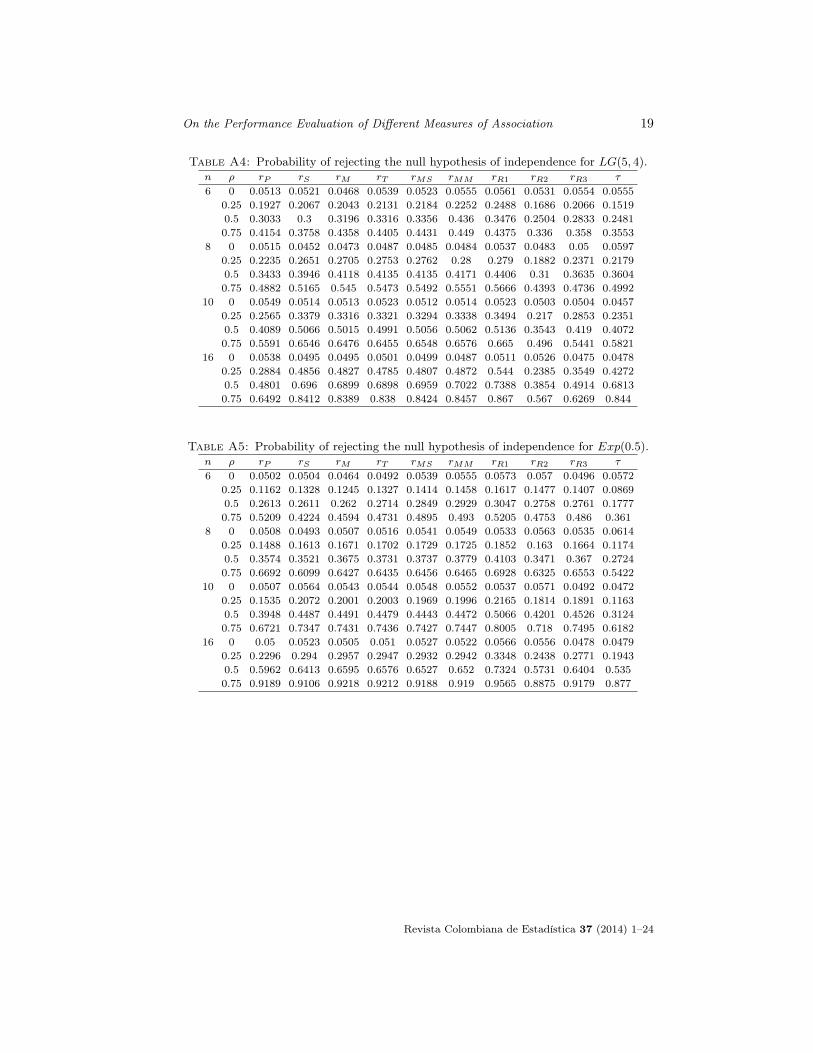
On the Performance Evaluation of Different Measures of Association 19
Table A4: Probability of rejecting the null hypothesis of independence for LG(5, 4).n ρ rP rS rM rT rMS rMM rR1 rR2 rR3 τ
6 0 0.0513 0.0521 0.0468 0.0539 0.0523 0.0555 0.0561 0.0531 0.0554 0.05550.25 0.1927 0.2067 0.2043 0.2131 0.2184 0.2252 0.2488 0.1686 0.2066 0.15190.5 0.3033 0.3 0.3196 0.3316 0.3356 0.436 0.3476 0.2504 0.2833 0.24810.75 0.4154 0.3758 0.4358 0.4405 0.4431 0.449 0.4375 0.336 0.358 0.3553
8 0 0.0515 0.0452 0.0473 0.0487 0.0485 0.0484 0.0537 0.0483 0.05 0.05970.25 0.2235 0.2651 0.2705 0.2753 0.2762 0.28 0.279 0.1882 0.2371 0.21790.5 0.3433 0.3946 0.4118 0.4135 0.4135 0.4171 0.4406 0.31 0.3635 0.36040.75 0.4882 0.5165 0.545 0.5473 0.5492 0.5551 0.5666 0.4393 0.4736 0.4992
10 0 0.0549 0.0514 0.0513 0.0523 0.0512 0.0514 0.0523 0.0503 0.0504 0.04570.25 0.2565 0.3379 0.3316 0.3321 0.3294 0.3338 0.3494 0.217 0.2853 0.23510.5 0.4089 0.5066 0.5015 0.4991 0.5056 0.5062 0.5136 0.3543 0.419 0.40720.75 0.5591 0.6546 0.6476 0.6455 0.6548 0.6576 0.665 0.496 0.5441 0.5821
16 0 0.0538 0.0495 0.0495 0.0501 0.0499 0.0487 0.0511 0.0526 0.0475 0.04780.25 0.2884 0.4856 0.4827 0.4785 0.4807 0.4872 0.544 0.2385 0.3549 0.42720.5 0.4801 0.696 0.6899 0.6898 0.6959 0.7022 0.7388 0.3854 0.4914 0.68130.75 0.6492 0.8412 0.8389 0.838 0.8424 0.8457 0.867 0.567 0.6269 0.844
Table A5: Probability of rejecting the null hypothesis of independence for Exp(0.5).n ρ rP rS rM rT rMS rMM rR1 rR2 rR3 τ
6 0 0.0502 0.0504 0.0464 0.0492 0.0539 0.0555 0.0573 0.057 0.0496 0.05720.25 0.1162 0.1328 0.1245 0.1327 0.1414 0.1458 0.1617 0.1477 0.1407 0.08690.5 0.2613 0.2611 0.262 0.2714 0.2849 0.2929 0.3047 0.2758 0.2761 0.17770.75 0.5209 0.4224 0.4594 0.4731 0.4895 0.493 0.5205 0.4753 0.486 0.361
8 0 0.0508 0.0493 0.0507 0.0516 0.0541 0.0549 0.0533 0.0563 0.0535 0.06140.25 0.1488 0.1613 0.1671 0.1702 0.1729 0.1725 0.1852 0.163 0.1664 0.11740.5 0.3574 0.3521 0.3675 0.3731 0.3737 0.3779 0.4103 0.3471 0.367 0.27240.75 0.6692 0.6099 0.6427 0.6435 0.6456 0.6465 0.6928 0.6325 0.6553 0.5422
10 0 0.0507 0.0564 0.0543 0.0544 0.0548 0.0552 0.0537 0.0571 0.0492 0.04720.25 0.1535 0.2072 0.2001 0.2003 0.1969 0.1996 0.2165 0.1814 0.1891 0.11630.5 0.3948 0.4487 0.4491 0.4479 0.4443 0.4472 0.5066 0.4201 0.4526 0.31240.75 0.6721 0.7347 0.7431 0.7436 0.7427 0.7447 0.8005 0.718 0.7495 0.6182
16 0 0.05 0.0523 0.0505 0.051 0.0527 0.0522 0.0566 0.0556 0.0478 0.04790.25 0.2296 0.294 0.2957 0.2947 0.2932 0.2942 0.3348 0.2438 0.2771 0.19430.5 0.5962 0.6413 0.6595 0.6576 0.6527 0.652 0.7324 0.5731 0.6404 0.5350.75 0.9189 0.9106 0.9218 0.9212 0.9188 0.919 0.9565 0.8875 0.9179 0.877
Revista Colombiana de Estadística 37 (2014) 1–24
20 Muhammad Riaz, Shahzad Munir & Zahid Asghar
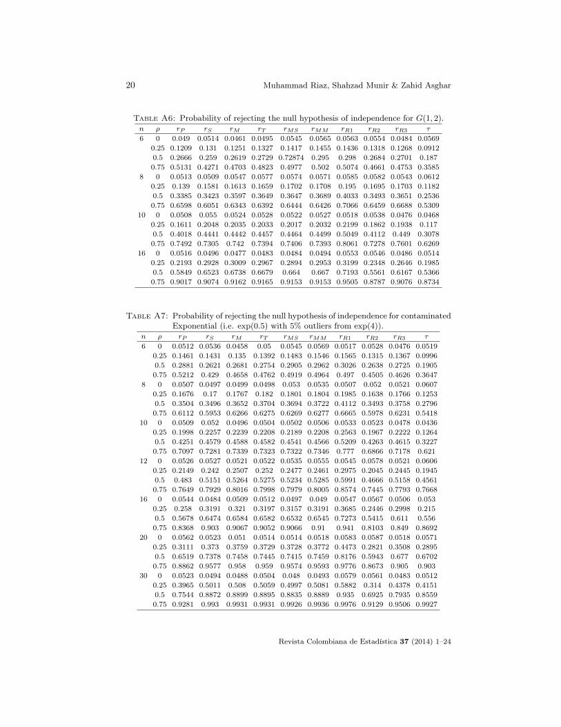
Table A6: Probability of rejecting the null hypothesis of independence for G(1, 2).n ρ rP rS rM rT rMS rMM rR1 rR2 rR3 τ
6 0 0.049 0.0514 0.0461 0.0495 0.0545 0.0565 0.0563 0.0554 0.0484 0.05690.25 0.1209 0.131 0.1251 0.1327 0.1417 0.1455 0.1436 0.1318 0.1268 0.09120.5 0.2666 0.259 0.2619 0.2729 0.72874 0.295 0.298 0.2684 0.2701 0.1870.75 0.5131 0.4271 0.4703 0.4823 0.4977 0.502 0.5074 0.4661 0.4753 0.3585
8 0 0.0513 0.0509 0.0547 0.0577 0.0574 0.0571 0.0585 0.0582 0.0543 0.06120.25 0.139 0.1581 0.1613 0.1659 0.1702 0.1708 0.195 0.1695 0.1703 0.11820.5 0.3385 0.3423 0.3597 0.3649 0.3647 0.3689 0.4033 0.3493 0.3651 0.25360.75 0.6598 0.6051 0.6343 0.6392 0.6444 0.6426 0.7066 0.6459 0.6688 0.5309
10 0 0.0508 0.055 0.0524 0.0528 0.0522 0.0527 0.0518 0.0538 0.0476 0.04680.25 0.1611 0.2048 0.2035 0.2033 0.2017 0.2032 0.2199 0.1862 0.1938 0.1170.5 0.4018 0.4441 0.4442 0.4457 0.4464 0.4499 0.5049 0.4112 0.449 0.30780.75 0.7492 0.7305 0.742 0.7394 0.7406 0.7393 0.8061 0.7278 0.7601 0.6269
16 0 0.0516 0.0496 0.0477 0.0483 0.0484 0.0494 0.0553 0.0546 0.0486 0.05140.25 0.2193 0.2928 0.3009 0.2967 0.2894 0.2953 0.3199 0.2348 0.2646 0.19850.5 0.5849 0.6523 0.6738 0.6679 0.664 0.667 0.7193 0.5561 0.6167 0.53660.75 0.9017 0.9074 0.9162 0.9165 0.9153 0.9153 0.9505 0.8787 0.9076 0.8734
Table A7: Probability of rejecting the null hypothesis of independence for contaminatedExponential (i.e. exp(0.5) with 5% outliers from exp(4)).
n ρ rP rS rM rT rMS rMM rR1 rR2 rR3 τ
6 0 0.0512 0.0536 0.0458 0.05 0.0545 0.0569 0.0517 0.0528 0.0476 0.05190.25 0.1461 0.1431 0.135 0.1392 0.1483 0.1546 0.1565 0.1315 0.1367 0.09960.5 0.2881 0.2621 0.2681 0.2754 0.2905 0.2962 0.3026 0.2638 0.2725 0.19050.75 0.5212 0.429 0.4658 0.4762 0.4919 0.4964 0.497 0.4505 0.4626 0.3647
8 0 0.0507 0.0497 0.0499 0.0498 0.053 0.0535 0.0507 0.052 0.0521 0.06070.25 0.1676 0.17 0.1767 0.182 0.1801 0.1804 0.1985 0.1638 0.1766 0.12530.5 0.3504 0.3496 0.3652 0.3704 0.3694 0.3722 0.4112 0.3493 0.3758 0.27960.75 0.6112 0.5953 0.6266 0.6275 0.6269 0.6277 0.6665 0.5978 0.6231 0.5418
10 0 0.0509 0.052 0.0496 0.0504 0.0502 0.0506 0.0533 0.0523 0.0478 0.04360.25 0.1998 0.2257 0.2239 0.2208 0.2189 0.2208 0.2563 0.1967 0.2222 0.12640.5 0.4251 0.4579 0.4588 0.4582 0.4541 0.4566 0.5209 0.4263 0.4615 0.32270.75 0.7097 0.7281 0.7339 0.7323 0.7322 0.7346 0.777 0.6866 0.7178 0.621
12 0 0.0526 0.0527 0.0521 0.0522 0.0535 0.0555 0.0545 0.0578 0.0521 0.06060.25 0.2149 0.242 0.2507 0.252 0.2477 0.2461 0.2975 0.2045 0.2445 0.19450.5 0.483 0.5151 0.5264 0.5275 0.5234 0.5285 0.5991 0.4666 0.5158 0.45610.75 0.7649 0.7929 0.8016 0.7998 0.7979 0.8005 0.8574 0.7445 0.7793 0.7668
16 0 0.0544 0.0484 0.0509 0.0512 0.0497 0.049 0.0547 0.0567 0.0506 0.0530.25 0.258 0.3191 0.321 0.3197 0.3157 0.3191 0.3685 0.2446 0.2998 0.2150.5 0.5678 0.6474 0.6584 0.6582 0.6532 0.6545 0.7273 0.5415 0.611 0.5560.75 0.8368 0.903 0.9067 0.9052 0.9066 0.91 0.941 0.8103 0.849 0.8692
20 0 0.0562 0.0523 0.051 0.0514 0.0514 0.0518 0.0583 0.0587 0.0518 0.05710.25 0.3111 0.373 0.3759 0.3729 0.3728 0.3772 0.4473 0.2821 0.3508 0.28950.5 0.6519 0.7378 0.7458 0.7445 0.7415 0.7459 0.8176 0.5943 0.677 0.67020.75 0.8862 0.9577 0.958 0.959 0.9574 0.9593 0.9776 0.8673 0.905 0.903
30 0 0.0523 0.0494 0.0488 0.0504 0.048 0.0493 0.0579 0.0561 0.0483 0.05120.25 0.3965 0.5011 0.508 0.5059 0.4997 0.5081 0.5882 0.314 0.4378 0.41510.5 0.7544 0.8872 0.8899 0.8895 0.8835 0.8889 0.935 0.6925 0.7935 0.85590.75 0.9281 0.993 0.9931 0.9931 0.9926 0.9936 0.9976 0.9129 0.9506 0.9927
Revista Colombiana de Estadística 37 (2014) 1–24

On the Performance Evaluation of Different Measures of Association 21
Table A8: Probability of rejecting the null hypothesis of independence for contaminatedWeibull (i.e. W (0.5, 3) with 5% outliers from W (50, 100)).
n ρ rP rS rM rT rMS rMM rR1 rR2 rR3 τ
6 0 0.0563 0.0495 0.046 0.0507 0.05 0.054 0.0546 0.0595 0.0515 0.05360.25 0.1961 0.2037 0.2032 0.2134 0.216 0.224 0.2388 0.155 0.1866 0.14770.5 0.3217 0.2982 0.3185 0.3313 0.334 0.3422 0.3358 0.2338 0.265 0.2460.75 0.4379 0.377 0.4256 0.4351 0.4491 0.4536 0.4303 0.3343 0.3538 0.3604
8 0 0.053 0.0472 0.0537 0.0558 0.055 0.0559 0.052 0.0513 0.051 0.06210.25 0.2091 0.2595 0.2674 0.2699 0.2681 0.2715 0.2878 0.1903 0.2486 0.21580.5 0.3449 0.3958 0.4105 0.412 0.4158 0.4193 0.4391 0.3224 0.3734 0.35590.75 0.4918 0.5282 0.5584 0.5593 0.562 0.5642 0.5971 0.4593 0.5004 0.5103
10 0 0.056 0.0529 0.0543 0.0545 0.0536 0.0542 0.0546 0.05 0.0468 0.04390.25 0.2245 0.3157 0.3159 0.3144 0.3178 0.3194 0.348 0.2076 0.278 0.22780.5 0.3897 0.4948 0.4944 0.4923 0.4935 0.499 0.5287 0.3585 0.4245 0.40660.75 0.5662 0.6507 0.6523 0.649 0.6548 0.6575 0.6933 0.52 0.5715 0.5827
12 0 0.0543 0.047 0.0494 0.0486 0.0485 0.0487 0.0541 0.0526 0.0499 0.06160.25 0.2444 0.3695 0.3706 0.3651 0.3703 0.3758 0.4141 0.2037 0.291 0.32820.5 0.4294 0.5665 0.5735 0.5709 0.5747 0.5803 0.6293 0.3733 0.458 0.54570.75 0.632 0.7293 0.7405 0.7376 0.7445 0.7495 0.7476 0.542 0.573 0.7277
16 0 0.0551 0.0473 0.0486 0.048 0.046 0.0465 0.0583 0.0556 0.0466 0.0510.25 0.2573 0.474 0.4759 0.4675 0.4748 0.4796 0.5768 0.2373 0.3601 0.4030.5 0.4808 0.6826 0.6908 0.6864 0.6938 0.6978 0.7853 0.427 0.5396 0.65370.75 0.6946 0.8457 0.8518 0.8478 0.8587 0.8609 0.909 0.617 0.595 0.8397
20 0 0.0564 0.0494 0.0478 0.0467 0.0483 0.0478 0.0561 0.0553 0.0421 0.05240.25 0.2922 0.5503 0.5525 0.5436 0.5526 0.5592 0.6545 0.2324 0.3813 0.50660.5 0.5422 0.7837 0.7879 0.783 0.7933 0.7966 0.855 0.4396 0.5745 0.77110.75 0.7668 0.9111 0.9201 0.914 0.921 0.9232 0.9549 0.6459 0.7369 0.9212
30 0 0.0536 0.0489 0.0514 0.0507 0.0506 0.0508 0.0587 0.0591 0.0471 0.05260.25 0.3259 0.7257 0.7253 0.7191 0.7315 0.7364 0.8438 0.2616 0.4875 0.69840.5 0.6594 0.9165 0.919 0.9132 0.9253 0.9272 0.9643 0.5166 0.7088 0.9250.75 0.8675 0.9824 0.9837 0.9825 0.9862 0.9868 0.9944 0.751 0.8554 0.9874
Revista Colombiana de Estadística 37 (2014) 1–24

22 Muhammad Riaz, Shahzad Munir & Zahid Asghar
Table A9: Probability of rejecting the null hypothesis of independence for contaminatedGamma (i.e. G(0.5, 3) with 5% outliers from G(4, 10)).
n ρ rP rS rM rT rMS rMM rR1 rR2 rR3 τ
6 0 0.0558 0.0511 0.0441 0.0488 0.0517 0.0532 0.058 0.0566 0.0505 0.0590.25 0.19 0.1675 0.1591 0.1692 0.1753 0.1797 0.1523 0.1316 0.129 0.1250.5 0.3134 0.273 0.282 0.2907 0.2992 0.3073 0.2931 0.2613 0.2716 0.21530.75 0.4823 0.3927 0.444 0.4511 0.459 0.4694 0.5315 0.5214 0.522 0.3621
8 0 0.0529 0.0468 0.0469 0.0508 0.0511 0.0513 0.052 0.0484 0.049 0.05680.25 0.2071 0.2201 0.2256 0.2268 0.2282 0.2306 0.2465 0.181 0.2228 0.16910.5 0.3542 0.3778 0.3964 0.4007 0.3973 0.3997 0.4075 0.3271 0.361 0.33310.75 0.5516 0.5551 0.5834 0.5872 0.5885 0.5828 0.604 0.5069 0.5346 0.5147
10 0 0.05 0.0516 0.0511 0.0506 0.0505 0.0506 0.0542 0.0567 0.055 0.04510.25 0.2311 0.2757 0.2692 0.2698 0.2682 0.2727 0.3208 0.2124 0.2766 0.18620.5 0.4032 0.4814 0.4774 0.4768 0.4736 0.4796 0.5083 0.3796 0.4294 0.36870.75 0.6091 0.6786 0.683 0.6836 0.6855 0.6884 0.7269 0.5859 0.6264 0.5994
12 0 0.0537 0.0492 0.0497 0.0523 0.0488 0.0495 0.0567 0.0563 0.056 0.06080.25 0.2629 0.3188 0.3159 0.3134 0.312 0.3142 0.3794 0.2291 0.3031 0.26380.5 0.4416 0.534 0.5377 0.533 0.5336 0.5404 0.6092 0.4245 0.4915 0.50290.75 0.6671 0.7588 0.7627 0.7605 0.7649 0.7715 0.8115 0.63 0.6743 0.7449
16 0 0.0512 0.048 0.0465 0.0475 0.0473 0.047 0.0583 0.0577 0.0549 0.05570.25 0.3053 0.4014 0.3947 0.391 0.3895 0.3965 0.4578 0.2491 0.3418 0.31810.5 0.5198 0.6707 0.6731 0.6677 0.6677 0.6781 0.7086 0.4612 0.5372 0.6130.75 0.7337 0.8729 0.8735 0.8728 0.8705 0.878 0.909 0.686 0.7425 0.8595
20 0 0.0543 0.0529 0.0525 0.054 0.053 0.052 0.0552 0.058 0.05 0.05330.25 0.3422 0.4829 0.472 0.4699 0.4691 0.4771 0.517 0.2521 0.3698 0.40490.5 0.5784 0.7569 0.7588 0.7547 0.752 0.7604 0.7905 0.4822 0.578 0.73280.75 0.7558 0.9349 0.9339 0.9332 0.932 0.9371 0.9521 0.7193 0.7757 0.9307
30 0 0.0537 0.0476 0.0516 0.0505 0.0522 0.0513 0.0578 0.0599 0.0436 0.05030.25 0.4102 0.6268 0.6133 0.6109 0.6127 0.6239 0.6714 0.2853 0.4545 0.5810.5 0.6641 0.9085 0.9049 0.9024 0.9024 0.9096 0.9171 0.5486 0.6815 0.90590.75 0.8317 0.9894 0.9891 0.9887 0.9886 0.9909 0.992 0.769 0.8385 0.9898
Revista Colombiana de Estadística 37 (2014) 1–24

On the Performance Evaluation of Different Measures of Association 23
Table A10: Probability of rejecting the null hypothesis of independence for HN(0, 1).n ρ rP rS rM rT rMS rMM rR1 rR2 rR3 τ
6 0 0.0527 0.055 0.0474 0.05 0.0572 0.0569 0.0547 0.0587 0.0502 0.04890.25 0.1081 0.1107 0.1053 0.1129 0.1219 0.1241 0.1279 0.1255 0.1125 0.07190.5 0.2726 0.2383 0.2354 0.245 0.2601 0.2619 0.2794 0.2628 0.2608 0.16030.75 0.5664 0.4319 0.4686 0.4788 0.4972 0.5033 0.5393 0.5163 0.518 0.3526
8 0 0.0501 0.0476 0.0477 0.0488 0.0507 0.0502 0.0523 0.0556 0.049 0.0620.25 0.1431 0.1374 0.1417 0.1429 0.1478 0.1473 0.1498 0.1439 0.14 0.10340.5 0.3078 0.3244 0.3394 0.3422 0.35 0.3526 0.3495 0.3381 0.332 0.24370.75 0.7315 0.6296 0.6601 0.6632 0.6649 0.6655 0.7133 0.6879 0.7012 0.5427
10 0 0.0513 0.0565 0.0545 0.0541 0.056 0.0549 0.0538 0.0501 0.0481 0.04980.25 0.16 0.1748 0.1704 0.1715 0.1682 0.1666 0.1784 0.1693 0.1661 0.09460.5 0.4419 0.4141 0.4185 0.4176 0.4165 0.4168 0.455 0.4234 0.4336 0.27480.75 0.8075 0.7678 0.7817 0.7811 0.781 0.7791 0.8225 0.7998 0.8116 0.6435
16 0 0.0553 0.0483 0.0463 0.0465 0.0467 0.0475 0.0585 0.057 0.0535 0.04910.25 0.2478 0.2443 0.2473 0.2468 0.2452 0.2443 0.2796 0.2526 0.2591 0.15320.5 0.6544 0.6136 0.633 0.6339 0.624 0.6253 0.695 0.6351 0.6625 0.49690.75 0.9678 0.9398 0.9496 0.9486 0.9462 0.9465 0.9681 0.952 0.9603 0.896
Table A11: Probability of rejecting the null hypothesis of independence for U(0, 1).n ρ rP rS rM rT rMS rMM rR1 rR2 rR3 τ
6 0 0.0504 0.0472 0.0433 0.0452 0.0513 0.0503 0.0657 0.0623 0.0572 0.06070.25 0.1215 0.1108 0.1071 0.1127 0.1216 0.1228 0.1418 0.1389 0.1287 0.07260.5 0.2433 0.2029 0.2059 0.2118 0.2259 0.2276 0.2719 0.258 0.2523 0.13670.75 0.602 0.4506 0.4673 0.4821 0.5034 0.5062 0.5819 0.569 0.5703 0.3385
8 0 0.0472 0.0455 0.0458 0.0472 0.049 0.0492 0.058 0.0591 0.0577 0.06020.25 0.1422 0.127 0.1331 0.1344 0.1376 0.1375 0.1646 0.1541 0.1524 0.10090.5 0.3514 0.2906 0.3082 0.3103 0.3123 0.3136 0.3572 0.3501 0.3472 0.21650.75 0.7977 0.6619 0.6967 0.7004 0.7025 0.6989 0.766 0.7746 0.7777 0.5501
10 0 0.048 0.0502 0.0491 0.0506 0.0493 0.0481 0.0532 0.0546 0.0502 0.04640.25 0.1683 0.1614 0.1581 0.1577 0.1561 0.1564 0.1838 0.1834 0.1773 0.08440.5 0.4359 0.389 0.3944 0.3956 0.3928 0.3905 0.4428 0.4507 0.4433 0.2440.75 0.9033 0.8261 0.8388 0.8403 0.8367 0.836 0.8745 0.8883 0.8876 0.6622
16 0 0.0494 0.0501 0.0469 0.0485 0.0492 0.0479 0.0542 0.0544 0.0529 0.05220.25 0.2319 0.2183 0.2167 0.2163 0.2135 0.2129 0.2358 0.2358 0.2308 0.13080.5 0.6541 0.585 0.605 0.604 0.5972 0.5959 0.6205 0.6535 0.6394 0.44230.75 0.9904 0.9732 0.9779 0.978 0.9759 0.9761 0.9818 0.9874 0.9871 0.9407
Revista Colombiana de Estadística 37 (2014) 1–24

24 Muhammad Riaz, Shahzad Munir & Zahid Asghar
Table A12: Probability of rejecting the null hypothesis of independence for Mixed Nor-mal (i.e. N(0, 1) with probability 0.95 and N(0, 400 with probability 0.05).
n ρ rP rS rM rT rMS rMM rR1 rR2 rR3 τ
6 0 0.0522 0.0512 0.0471 0.0499 0.0537 0.0543 0.0662 0.0675 0.0628 0.05750.25 0.1265 0.1104 0.1037 0.1106 0.121 0.1222 0.1382 0.1362 0.1287 0.07840.5 0.2723 0.2205 0.2197 0.2307 0.2459 0.2487 0.2811 0.2837 0.2702 0.15930.75 0.611 0.4506 0.471 0.4927 0.5139 0.5145 0.5607 0.5623 0.5584 0.3533
8 0 0.0463 0.0468 0.0476 0.0493 0.0499 0.0499 0.0591 0.0607 0.0539 0.05860.25 0.142 0.1262 0.1309 0.135 0.1365 0.1361 0.168 0.1717 0.1606 0.09840.5 0.3834 0.3081 0.3226 0.3296 0.3326 0.3328 0.3867 0.3871 0.3852 0.23780.75 0.7721 0.6394 0.6697 0.6769 0.6762 0.6756 0.7445 0.7452 0.7473 0.558
10 0 0.0472 0.0517 0.0491 0.0485 0.0484 0.049 0.0587 0.0615 0.0564 0.04840.25 0.1734 0.1606 0.1589 0.1594 0.1623 0.1609 0.1949 0.1946 0.1868 0.09290.5 0.4634 0.4077 0.4045 0.408 0.4086 0.4062 0.4658 0.4627 0.4564 0.26270.75 0.8661 0.7901 0.7991 0.8016 0.7986 0.7944 0.8536 0.8557 0.8569 0.6404
16 0 0.05 0.0528 0.053 0.0533 0.0538 0.0544 0.0582 0.0595 0.0561 0.05020.25 0.238 0.2148 0.2168 0.2158 0.216 0.2146 0.2521 0.2513 0.247 0.13990.5 0.6723 0.6033 0.6161 0.6174 0.6122 0.6135 0.6501 0.6524 0.6528 0.46550.75 0.9775 0.951 0.9569 0.9568 0.9552 0.9549 0.9709 0.971 0.9731 0.9109
Table A13: Probability of rejecting the null hypothesis of independence for L(0.5, 3).n ρ rP rS rM rT rMS rMM rR1 rR2 rR3 τ
6 0 0.0503 0.0515 0.0435 0.0503 0.0536 0.0548 0.0628 0.065 0.0575 0.05880.25 0.1396 0.1259 0.1141 0.1252 0.1335 0.1362 0.1661 0.1534 0.1452 0.08530.5 0.3145 0.2439 0.2422 0.2604 0.2753 0.2768 0.3361 0.3201 0.317 0.17640.75 0.6045 0.4345 0.4734 0.4919 0.5058 0.5058 0.5602 0.5498 0.5543 0.3735
8 0 0.0528 0.0481 0.0465 0.0497 0.0506 0.0514 0.0652 0.0646 0.0559 0.06020.25 0.1712 0.152 0.1567 0.165 0.1668 0.1681 0.209 0.1898 0.1914 0.11510.5 0.4058 0.3317 0.3469 0.3542 0.3566 0.3558 0.4487 0.4065 0.4192 0.25890.75 0.7375 0.6085 0.641 0.6483 0.6479 0.6473 0.7465 0.7065 0.723 0.5538
10 0 0.0495 0.0487 0.0447 0.047 0.0468 0.0462 0.0666 0.0682 0.0585 0.04670.25 0.1904 0.1895 0.1845 0.1904 0.1899 0.1892 0.2397 0.2089 0.21 0.10740.5 0.4806 0.4303 0.4328 0.4359 0.4363 0.4359 0.5409 0.4761 0.5031 0.29830.75 0.8313 0.7533 0.7566 0.7561 0.7583 0.7573 0.8397 0.8053 0.8213 0.6283
16 0 0.0491 0.0458 0.0438 0.0445 0.0455 0.046 0.0667 0.0661 0.059 0.05150.25 0.2535 0.2572 0.2585 0.2588 0.259 0.263 0.3378 0.2773 0.2969 0.1740.5 0.656 0.6127 0.6236 0.6223 0.625 0.6227 0.7213 0.6377 0.7661 0.51040.75 0.9504 0.9197 0.9225 0.9234 0.9235 0.9234 0.9602 0.9386 0.9495 0.8766
Revista Colombiana de Estadística 37 (2014) 1–24