Online ISSN: 2367-5357 DOI: 10.7546/itc-2019-0017 Traffic ...

Information Technologies 4 2019 12 and Control

Online ISSN: 2367-5357

DOI: 10.7546/itc-2019-0017

Traffic Management

of Urban Network

by Bi-level Optimization

K. Stoilova, T. Stoilov, K. Pavlova

Key Words: Traffic control; transportation behavior; urban

network of crossroad traffic lights; hierarchical approach; bi-level

optimization.

Abstract. A city network of crossroad sections is under

consideration in order to reduce the traffic jams, the traffic queue

lengths in front of the junctions, and to increase the outgoing

traffic flows. The implementation of these goals is achieved by

application of hierarchical approach. A bi-level optimization is

applied for finding the optimal control parameters as solutions of

appropriate optimization problems, hierarchically interconnected.

The numerical simulations’ results show improvement of the

traffic’s characteristics.

1. Introduction

The traffic management is wide discussed problem for

many years because of its importance in our everyday life.

The actuality of this topic is caused of its complexity and

attempts of the world’s scientific society to be applied the

modern theoretical and simulation achievements [1, 2].

An analysis of the traffic control strategies is presented in

[3, 4]. The main control parameters, used for the traffic

management in urban areas are the traffic light cycle

duration, the green light duration of the traffic light cycle,

and the traffic lights offset in a network of crossroads.

Usually, the presented papers concern optimization of only

one of these control parameters. Optimization problem

using only one control parameter (the green light duration)

is considered in [5] for the design of traffic lights plans and

for minimization of the queue lengths in front of the traffic

lights based on the store-and-forward model in [6].

Optimal signal settings only for the traffic lights are

considered in [7-9].

The above researches aim solutions of one criterion

optimization problems. In this paper we are solving two-

criterion optimization problem based on the hierarchical

system’s theory. Because of the complexity of the multilevel

manner of optimization, practical application has the bi-

level approach where two-level hierarchical system is

considered. The bi-level optimization extends the

optimization environment (goal, parameters and

constraints) by the embedded philosophy of its functionality

through interconnections between the both optimization

problems.

2. Bi-level Optimization

The bi-level optimization targets optimization of two

interconnected optimization problems. The solution of the

lower-level problem is sent to the upper level problem

where this optimal solution is regarded as a parameter for

the upper level optimization problem. The analogical is the

interconnection between the upper and lower level

optimization problem. This hierarchical approach is chosen

in our research because it allows smaller optimization

problems to be solved easier on each level and because of

their interconnections more complex optimization problem

is solved. In practice, instead of two independent sub-

problems, one global problem with two goals is solved.

This complex problem has more parameters

(the optimization variables of the lower and upper level

optimization problems), larger number of constraints

(the resources of the both optimization problems) and

satisfaction of two goal functions. The interconnection

between the both optimization problems leads to

optimization of more goals, satisfying more constraints and

including more parameters in comparison with the classical

optimization of two optimization problems twice.

This tendency of the application of the bi-level optimization

is analyzed in [10, 11]. Nevertheless the difficulties of the

usage of the bi-level approach, it is applied in different

domains nowadays because of its triple advantages,

mentioned above. The bi-level optimization is applied in

[12] for logistic purposes minimizing the customers’ costs

and satisfying their demands. Another logistic problem is

solved by bi-level optimization in [13] where m sources


have to be distributed to n destinations. Different priorities

are assigned to the destinations by hierarchical manner.

In [14] the bi-level optimization is applied for locating of

logistics.

In [15] the bi-level approach is applied to the public

transport. The time interval among the different buses is

optimized on the upper level having in mind their capacities.

The lower level determines the user’s preferences for routes.

Similar problem is considered in [16] where the upper level

minimizes the travel costs and lower level – bus

transportation scheme.

This short overview shows that the bi-level

optimization has bigger instrumentation to consider more

requirements, which is the main reason to be applied for

decision making problems, management of logistics

problems and transportation. These advantages of the bi-

level approach are due to the inclusion of more parameters,

constraints and goals of these interconnected optimization

problems. For these reasons the bi-level approach is applied

in this research for improving the traffic characteristics of

urban network of crossroads.

3. Determination of the optimization

problems

The architecture of the city network is presented in

figure 1. We consider a network with five crossroad sections

and the goal is to decrease the queue lengths in horizontal

direction from West to East and vise versa where is the main

traffic flow in Sofia. For the network the traffic lights cycles

are cj, j = 1, …, 5. It includes green, amber and red light.

The amber light is 0.1 of the traffic light cycle. The traffic

light cycle is c1 for the first crossroad section. The green

light duration for the first junction is u1 in vertical direction.

For the horizontal direction the green light duration is

(0.9c1 – u1). The queue lengths are xi, i = 1, …, 18, figure 1.

We suppose that for the first crossroad section the

saturations are S1 in horizontal and S2 in vertical direction.

For the next four junctions the saturations are respectively

S3 – S4, S5 – S6, S7 – S8, and S9 – S10. The distance and density

between the first and second traffic lights are respectively

L1 and ρ1. For the next three parts they are respectively L2

and ρ2, L3 and ρ3, L4 and ρ4. The outgoing flows are qk,

k = 1, …, 8, figure 1.

Figure 1. Urban traffic network

3.1. Determination of the lower-level

optimization problem The goal of the lower-level problem is to minimize the

queue lengths in front of the traffic lights. We choose a

quadratic optimization goal function with arguments queue

lengths and the green light durations of the all five junctions

of the network. The constraints of this problem are based on

the store – and – forward model, applied for the all 18 queue

lengths. The lower-level problem is

(1) min𝑖=1,…,18𝑗=1,…,5

(𝑥𝑖2 + 𝑢𝑗

2)

subject to

(2) 𝑥1 − 𝑆1𝑢1 + 0.9𝑆1𝑐1 ≤ 𝑥10+ 𝑥1𝑖𝑛

𝑥2 + 𝑆2𝑢1 ≤ 𝑥20+ 𝑥2𝑖𝑛

𝑥3 + 𝑆2𝑢1 ≤ 𝑥30+ 𝑥3𝑖𝑛

𝑥4 − 𝑆1𝑢1 + 𝑆3𝑢2 + 0.9𝑆1𝑐1 − 0.9𝑆3𝑐2 ≤ 𝑥40

𝑥5 + 𝑆1𝑢1 − 𝑆3𝑢2 − 0.9𝑆1𝑐1 + 0.9𝑆3𝑐2 ≤ 𝑥50

𝑥6 + 𝑆4𝑢2 ≤ 𝑥60+ 𝑥6𝑖𝑛

𝑥7 + 𝑆4𝑢2 ≤ 𝑥70+ 𝑥7𝑖𝑛

𝑥8−𝑆3𝑢2 + 𝑆5𝑢3 + 0.9𝑆3𝑐2 − 0.9𝑆5𝑐3 ≤ 𝑥80

𝑥9+𝑆3𝑢2 − 𝑆5𝑢3 − 0.9𝑆3𝑐2 + 0.9𝑆5𝑐3 ≤ 𝑥90

𝑥10 + 𝑆6𝑢3 ≤ 𝑥100+ 𝑥10𝑖𝑛

𝑥11 + 𝑆6𝑢3 ≤ 𝑥110+ 𝑥11𝑖𝑛

x1 x5 x9 x13 x16

x3

x2

x4 x7

x6

x8 x11

x10

x12

x14 x15

x17

x18

S1 x1 S2 S3 S4 S5 S6 S7

S8

S9 S10

u1 u2 u3 u4 u5

L1/ ρ1 L2/ ρ2 L3/ ρ3 L4/ ρ4

q2 q3 q4 q1

q5 q6 q7 q8


𝑥12 − 𝑆5𝑢3+𝑆7𝑢4 + 0.9𝑆5𝑐3 − 0.9𝑆7𝑐4 ≤ 𝑥120

𝑥13 + 𝑆5𝑢3−𝑆7𝑢4 − 0.9𝑆5𝑐3 + 0.9𝑆7𝑐4 ≤ 𝑥130

𝑥14 + 𝑆8𝑢4 ≤ 𝑥140+ 𝑥14𝑖𝑛

𝑥15 − 𝑆7𝑢4 + 𝑆9𝑢5 + 0.9𝑆7𝑐4 − 0.9𝑆9𝑐5 ≤ 𝑥150

𝑥16 + 𝑆7𝑢4 − 𝑆9𝑢5 − 0.9𝑆7𝑐4 + 0.9𝑆9𝑐5 ≤ 𝑥160

𝑥17 + 𝑆10𝑢5 ≤ 𝑥170+ 𝑥17𝑖𝑛

𝑥18 − 𝑆91𝑢5 + 0.9𝑆9𝑐5 ≤ 𝑥180+ 𝑥18𝑖𝑛

.

Problem (1) can be presented in vector form like

(3) min𝑥,𝑢

(𝑥′𝑄1𝑥 + 𝑢′𝑄2𝑢)

subject to

(4) 𝐴1𝑥+𝐴2𝑢 + 𝐴3𝑦 ≤ 𝐵,

where 𝑄1, 𝑄2, 𝐴1 are unit matrices:

(5) 𝑄1 = 𝑒𝑦𝑒(18,18), 𝑄2 = 𝑒𝑦𝑒(5,5),

𝐴1 = 𝑒𝑦𝑒(18,18),

(6) 𝐴2 =

‖

‖

‖

‖

‖

−𝑆1 0 0𝑆2 0 0𝑆2 0 0

0 00 00 0

−𝑆1 𝑆3 0𝑆1 −𝑆3 00 𝑆4 0

0 00 00 0

0 𝑆4 00 −𝑆3 𝑆5

0 𝑆3 −𝑆5

0 00 00 0

0 0 𝑆6

0 0 𝑆6

0 0 −𝑆5

0 00 0𝑆7 0

0 0 𝑆5

0 0 00 0 0

−𝑆7 0𝑆8 0

−𝑆7 𝑆9

0 0 00 0 00 0 0

𝑆7 −𝑆9

0 𝑆10

0 −𝑆9

‖

‖

‖

‖

‖

(7) 𝐴3 =

‖

‖

‖

‖

‖

0.9𝑆1 0 00 0 00 0 0

0 00 00 0

0.9𝑆1 −0.9𝑆3 0−0.9𝑆1 0.9𝑆3 0

0 0 0

0 00 00 0

0 0 00 0.9𝑆3 −0.9𝑆5

0 −0.9𝑆3 0.9𝑆5

0 00 00 0

0 0 00 0 00 0 0.9𝑆5

0 00 0

−0.9𝑆7 0

0 0 −0.9𝑆5

0 0 00 0 0

0.9𝑆7 0

0 00.9𝑆7 −0.9𝑆9

0 0 00 0 00 0 0

−0.9𝑆7 0.9𝑆9

0 00 0.9𝑆9

‖

‖

‖

‖

‖

(8) 𝐵 =

‖

‖

‖

‖

‖

‖

𝑥10+ 𝑥1𝑖𝑛



𝑥40

𝑥50



𝑥80

𝑥90

𝑥100+ 𝑥10𝑖𝑛

𝑥110+ 𝑥11𝑖𝑛

𝑥120

𝑥130

𝑥140+ 𝑥14𝑖𝑛

𝑥150

𝑥160

𝑥170+ 𝑥17𝑖𝑛

𝑥180+ 𝑥18𝑖𝑛

‖

‖

‖

‖

‖

‖

3.2. Determination of the upper-level

optimization problem The upper level optimization problem aims

maximization of the outgoing from the crossroad section

traffic flow. This model is based on the one of the main

transportation model – the continuity of the traffic flow,

which formalization is below. The traffic flow is proportional

to the traffic flow speed and traffic density and for the first

traffic flow between the first and second junction it is:

(10) 𝑞1 = 𝑣𝜌1.

The traffic flow speed is

(11) 𝑣 = 𝑣𝑓𝑟𝑒𝑒 (1 −𝜌1

𝜌1𝑚𝑎𝑥).

Substituting (11) in (10), it is obtained:


(12) 𝑞1 = 𝑣𝑓𝑟𝑒𝑒 (1 −𝜌1

𝜌1𝑚𝑎𝑥) 𝜌1.

The density 𝜌1 is formalized as relation between the

number of cars on the distance between the first and the

second traffic lights

(13) 𝜌1 = 𝑥5/𝐿1.

After substitution of (13) in (12) it is obtained

(14) 𝑞1=𝑣𝑓𝑟𝑒𝑒

𝐿1(𝑥5 −

𝑥52

𝜌1𝑚𝑎𝑥𝐿1).

As the constant 𝑣𝑓𝑟𝑒𝑒/𝐿1 does not influence the

optimization, we can ignore it. For simplification we denote

(15) 𝛽1 =1

𝜌1𝑚𝑎𝑥𝐿1

.

Then (14) can be written in the form

(16) 𝑞1 = (𝑥5 − 𝛽1𝑥52) .

Analogically, we can present the rest seven outgoing

flows like

(17) 𝑞2 = (𝑥9 − 𝛽2𝑥92)

𝑞3 = (𝑥13 − 𝛽3𝑥132 )

𝑞4 = (𝑥16 − 𝛽4𝑥162 )

𝑞5 = (𝑥15 − 𝛽4𝑥152 )

𝑞6 = (𝑥12 − 𝛽3𝑥122 )

𝑞7 = (𝑥8 − 𝛽2𝑥82)

𝑞8 = (𝑥4 − 𝛽1𝑥42).

The upper-level optimization targets maximization of

the eight outgoing traffic flows, which are functions of the

durations of the previous and next traffic light cycles:

(18) max𝑐𝑖,𝑖=1,…,5

{𝑞1(𝑐1, 𝑐2) + 𝑞2(𝑐2, 𝑐3) + 𝑞3(𝑐3, 𝑐4) +

𝑞4(𝑐4, 𝑐5) + 𝑞5(𝑐4, 𝑐5) + 𝑞6(𝑐3, 𝑐4) + 𝑞7(𝑐2, 𝑐3) +𝑞8(𝑐1, 𝑐2)}

By substituting (16) – (17) in the goal function (18), it

follows

(19) max𝑐𝑖,𝑖=1,…,5

{(𝑥5 − 𝛽1𝑥52) + (𝑥9 − 𝛽2𝑥9

2) + (𝑥13 −

𝛽1𝑥132 ) + (𝑥16 − 𝛽4𝑥16

2 ) + (𝑥15 − 𝛽4𝑥152 ) + (𝑥12 −

𝛽3𝑥122 ) + (𝑥8 − 𝛽2𝑥8

2) + (𝑥4 − 𝛽1𝑥42)}

subject to the constraints

(20) 𝑥5 = 𝑥50− 𝑆1𝑢1 + 𝑆3𝑢2 + 0.9𝑆1𝑐1 − 0.9𝑆3𝑐2

𝑥9 = 𝑥90− 𝑆3𝑢2 + 𝑆5𝑢3 + 0.9𝑆3𝑐2 − 0.9𝑆5𝑐3

𝑥13 = 𝑥130− 𝑆5𝑢3 + 𝑆7𝑢4 + 0.9𝑆5𝑐3 − 0.9𝑆7𝑐4

𝑥16 = 𝑥160− 𝑆7𝑢4 + 𝑆9𝑢5 + 0.9𝑆7𝑐4 − 0.9𝑆9𝑐5

𝑥15 = 𝑥150− 𝑆9𝑢5 + 𝑆7𝑢4 − 0.9𝑆7𝑐4 + 0.9𝑆9𝑐5

𝑥12 = 𝑥120− 𝑆7𝑢4 + 𝑆5𝑢3 − 0.9𝑆5𝑐3 + 0.9𝑆7𝑐4

𝑥8 = 𝑥50− 𝑆5𝑢3 + 𝑆3𝑢2 + 0.9𝑆5𝑐3 − 0.9𝑆3𝑐2

𝑥4 = 𝑥40− 𝑆3𝑢2 + 𝑆1𝑢1 − 0.9𝑆1𝑐1 + 0.9𝑆3𝑐2 .

The constraints (20) represent the outgoing flows from

the network’s junctions.

The goal function (19) can be presented in vector’s form:

(21) max𝑐𝑖,𝑖=1,…,5

{𝑐𝑇𝑄3𝑐 + 𝑐𝑇𝑄4𝑢 + 𝑢𝑇𝑄5𝑢 + 𝑄6𝑢 + 𝑄7𝑐}

where the matrices Q3 - Q7 are the following

𝑄3 =‖

‖

−1.62𝛽1𝑆12 1.62𝛽1𝑆1𝑆3 0

1.62𝛽1𝑆1𝑆3 −1.62(𝛽1 + 𝛽2)𝑆32 1.62𝛽2𝑆3𝑆5

0 1.62𝛽2𝑆3𝑆5 −1.62(𝛽2 + 𝛽3)𝑆52

0 00 0

1.62𝛽3𝑆5𝑆7 0

0 0 1.62𝛽3𝑆5𝑆7

0 0 0

−1.62(𝛽3 + 𝛽4)𝑆72 1.62𝛽4𝑆7𝑆9

1.62𝛽4𝑆7𝑆9 −1.62𝛽4𝑆92

‖

‖

𝑄4 =‖

‖

3.6𝛽1𝑆12 −3.6𝛽1𝑆1𝑆3 0

−3.6𝛽1𝑆1𝑆3 3.6(𝛽1 + 𝛽2)𝑆32 −3.6𝛽2𝑆3𝑆5

0 −3.6𝛽2𝑆3𝑆5 3.6(𝛽2 + 𝛽3)𝑆52

0 00 0

−3.6𝛽3𝑆5𝑆7 0

0 0 −3.6𝛽3𝑆5𝑆7

0 0 0

3.6(𝛽3 + 𝛽4)𝑆72 −3.6𝛽4𝑆7𝑆9

−3.6𝛽4𝑆7𝑆9 3.6𝛽4𝑆92

‖

‖


𝑄5 =‖

‖

−𝛽1𝑆12 2𝛽1𝑆1𝑆3 0

2𝛽1𝑆1𝑆3 −2(𝛽1 + 𝛽2)𝑆32 2𝛽2𝑆3𝑆5

0 2𝛽2𝑆3𝑆5 −2(𝛽2 + 𝛽3)𝑆52

0 00 0

2𝛽3𝑆5𝑆7 0

0 0 2𝛽3𝑆5𝑆7

0 0 0

−2(𝛽3 + 𝛽4)𝑆72 2𝛽4𝑆7𝑆9

2𝛽4𝑆7𝑆9 −2𝛽4𝑆92

‖

‖

𝑄6 = ‖2𝛽1(𝑥50

− 𝑥40)𝑆1 2[𝛽1(𝑥40

− 𝑥50) + 𝛽2(𝑥90

− 𝑥80)]𝑆3 2[𝛽2(𝑥80

− 𝑥90) + 𝛽3(𝑥130

− 𝑥120)]𝑆5

2[𝛽3(𝑥120− 𝑥130

) + 𝛽4(𝑥160− 𝑥150

)]𝑆7 2𝛽4(𝑥150− 𝑥160

)𝑆9

‖

𝑄7 = ‖1.8𝛽1(𝑥40

− 𝑥50)𝑆1 1.8[𝛽1(𝑥50

− 𝑥40) + 𝛽2(𝑥80

− 𝑥90)]𝑆3 1.8[𝛽2(𝑥90

− 𝑥80) + 𝛽3(𝑥120

− 𝑥130)]𝑆5

1.8[𝛽3(𝑥130− 𝑥120

) + 𝛽4(𝑥150− 𝑥160

)]𝑆7 1.8𝛽4(𝑥160− 𝑥150

)𝑆9

‖

The upper level optimization problem, formalized by

(19) - (20) aims optimal determining of the traffic lights cycles

of the all five traffic lights of the urban network. In this

problem the values of xi, i = 1, …, 18 and ui, i = 1, …, 5 are

received as optimal solutions from the lower level

optimization problem (3) - (4). The upper level’s optimization

problem finds as optimal solution the duration of the traffic

light cycles of the five traffic lights. These values of ci,

i = 1, …, 5 are sent to the lower level where they become

parameters of the lower-level optimization problem (3) - (4).

The iterative procedures continue till establishing

convergence of the solutions.

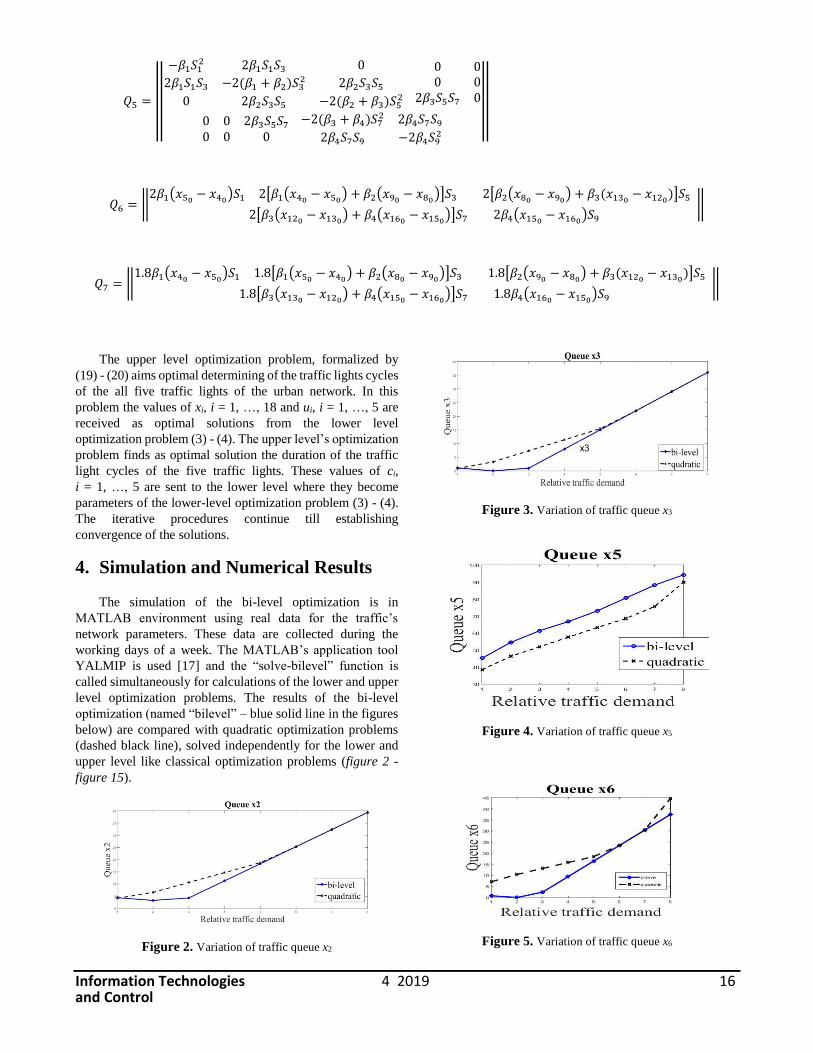
4. Simulation and Numerical Results

The simulation of the bi-level optimization is in

MATLAB environment using real data for the traffic’s

network parameters. These data are collected during the

working days of a week. The MATLAB’s application tool

YALMIP is used [17] and the “solve-bilevel” function is

called simultaneously for calculations of the lower and upper

level optimization problems. The results of the bi-level

optimization (named “bilevel” – blue solid line in the figures

below) are compared with quadratic optimization problems

(dashed black line), solved independently for the lower and

upper level like classical optimization problems (figure 2 -

figure 15).

Figure 2. Variation of traffic queue x2







Figure 16. Sum of all traffic queues

The traffic queues of the main direction West to East of

figure 1 (x5, x9, x13, x16) are a little bit bigger than by applying

quadratic optimization. However, the queue lengths of the

opposite main direction – from East to West (x8, x12, x15, x18)

have less values in comparison with the quadratic

optimization. Because the queue lengths after bi-level

optimization of the perpendicular directions (x2, x3, x6, x7, x10,

x11) are also smaller, we can conclude that the bi-level

optimization leads to better results. This is confirmed by the

sum of all traffic queues (figure 16) which shows lower level

of the queues after applying bi-level optimization.

The variation of the green lights durations are presented

in figures 17 - 20.

Figure 17. Variation of the green light duration u1






Because the current case is constant value of the green

light duration, in figures 17 - 21 their values are constant.

The solutions of the lower level optimization problem are the

queue lengths and the green light durations. It is seen in

figures 17 - 21 the different optimal solutions of the green

light durations for the all five crossroad sections.

The next experiments represent comparisons between

the bi-level optimization and solving classical quadratic

optimization problem with goal function green light

durations. The solutions of these problems are given

in figure 22.

Figure 22. Relative traffic demand by quadratic optimization

Figure 23 illustrates the variation of the green light

durations of the all five crossroad sections after bi-level

optimization.

Figure 23. Relative traffic demand by bi-level optimization

Figures 24 - 28 illustrate the dynamics of the green light

durations for each of the five traffic lights. In blue solid line

is the green light duration as solution of bi-level optimization

and the dashed black line is the green light duration applying

quadratic optimization.

Figure 24. Relative traffic demand for u1






The difference between the green lights dynsmics can

be explained with the different optimization problems. In the

classical optimization problem for finding the green light

duration only ui, i = 1, …, 5 are considered as arguments.

The solutions of the bi-level lower problem, which finds the

optimal ui, i = 1, …, 5 , except ui, i = 1, …, 5 are taking into

account the queue lengths in front of the junctions and the

traffic light cycles as optimal solutions from the upper level.

These interconnections lead to integration of more

arguments, constraints and goals, which result in improving

the traffic behavior.

5. Conclusion

This research presents the application of bi-level

optimization for improving traffic flow in urban area.

Formalization of the lower- and upper-level subproblems is

presented. The usage of the hierarchical optimization is

caused by its positive advantages like increasing the set of

optimization parameters, constraints and goal functions.

Instead of optimization of only one goal function with set of

parameters and constraints, the bi-level optimization allows

optimization of two goal functions, with wider set of

arguments and constraints, which leads to better results.

The lower level optimization goal is minimization of the

queue lengths in front of the junctions. The upper level

optimization problem targets maximization of the outgoing

from the junction traffic flow by optimizing the duration of

the traffic lights cycle. The calculated solutions of each

iteration are sent like parameters to the other optimization

level. In that manner is realized interconnection between the

both optimization problems which obtain two optimal

solutions of the both optimization problems, satisfying the

constraints of the both optimization problems. In that manner

by solving interacted simpler optimization problems is solved

complex optimization problem with larger sets of goals,

constraints and parameters. A real urban network is

considered with traffic data, collected by one week

measurements in working days. The simulation results are

compared on two folds: with the current state without

optimization and with classical optimization problems where

the goal and the sets of parameters and constraints are less in

comparison with the bi-level optimization. The received

results illustrate the improvement of the traffic behavior

when bi-level optimization is applied.

Acknowledgements

The research is funded by Project KP06-H37/6

“Modelling and optimization of urban traffic in network of

crossroads” with the Bulgarian Research Fund.

References

1. Li, L., Wen, D., Yao, D. A Survey of Traffic Control with

Vehicular Communications. – IEEE Transactions on Intelligent

Transportation Systems, 15, 2014, No. 1, 425–432.

2. Roess, R. P., Prassas, E. S., McShane, W. R. Traffic

Engineering. 5th Ed., Hoboken, NJ Pearson Education, 2019.

3. Wei, H., Zheng, G., Gayah, V., Li, Z. A Survey on Traffic Signal

Control Methods. Cornell University, 2020.

4. Papageorgiou, M., Diakaki, C., Dinopoulou, V., Kotsialos, A.,

Wang, Y. Review of Road Traffic Control Strategies, In Proc.

IEEE 91, 12, 2003, 2043–2067.

5. Eriskin, E., Karahancer, S., Terzi, S., Saltan, M. Optimization

of Traffic Signal Timing at Oversaturated Intersections Using

Elimination Pairing System. In 10th International Scientific

Conference Transbaltica, Transportation Science and

Technology, Procedia Engineering 187, 2017, 295–300.

6. Tettamanti, T., Varga, I. Peni, T. MPC in Urban Traffic

Management. In Zheng, T., Ed. Model Predictive Control,

InTechOpen, 2010.

7. Aboudolas, K., Papageorgiou, M., Kosmatopoulos, E. Store-

and-forward Based Methods for the Signal Control Problem in

Large-scale Congested Urban Road Networks. – Transportation

Research Part C, 1, 2009, 163–174.

8. Scheffle, R., Strehler, M. Optimizing Traffic Signal Settings for

Public Transport Priority, In D’Angelo, G., Dollevoet, T., Eds.

17th Workshop on Algorithmic Approaches for Transportation

Modelling, Optimization, and Systems (ATMOS), 2017, Article

No. 9; 9:1–9:15.

9. Ivanov, V. Monitoring of Urban Road Transport, In Proc. of

International Conference Аutomatics and Informatics, 2017,

135–141.

10. Hewage, K. N., Ruwanpura, J. Y. Optimization of Traffic Signal

Light Timing Using Simulation. In Ingalls, R. G., Rossetti, M.

D., Smith, J. S., Peters, B. A., Eds. Proc. 2004 Winter

Simulation Conference, 2004, 1428–1433.

11. Vicente, L. N., Calamai, P. H. Bilevel and Multilevel

Programming: A Bibliography Review. – J Glob Optim, 5,

1994, 291–306.

12. Colson, B., Marcotte, P., Savard, G. An Overview of Bilevel

Optimization. – J Ann Oper Res, 153, 2007, 235–256.

13. Khandelwal, S. A., Puri, M. C. Bilevel Time Minimizing

Transportation Problem. – J Discrete Optimization, 5, 2008, No.

4, 714–723.

14. Sun, H., Gao, Z., Wu, J. A Bi-level Programming Model and

Solution Algorithm for the Location of Logistics Distribution

Centers. – J Applied Mathematical Modelling, 32, 2008, No. 4,

610–616.

15. Arizti, A., Mauttone, A., Urquhart, M. E. A Bilevel Approach

to Frequency Optimization in Public Transportation Systems. In

18th Workshop on Algorithmic Approaches for Transportation

Modelling, Optimization, and Systems (ATMOS 2018), 65,

2008, 7:1–7:13.

https://www.researchgate.net/profile/Li_Li240?_sg%5B0%5D=i0r4awXsgSDkvf13elFeOkREiqmBCcPyEw6YHIHm7qmh3hVqo75td83Wl3Va80gyAL04kIc.17fahkd7dBk7qtaLf3R6w8l4o2sM5bsXUPIEWhrqdsDtjklb86zQExCrNHTH08dZ780BPd1ogjFiwyIX0VIODg&_sg%5B1%5D=p_i0cUZC8yPNH-pVS9eYgpUwDza0WbTCb9VGYl1omRdOfiGehmM0IETGBGIK49ThCcm07ls.qIUhRSr1cbYFvhFQFdE1L-_R0zw11AUnxWpkbV4Uy9Uj5LHj8LPCFlbtF_kZceUHdiV5tEDys9GaHYJTglpTbg

https://www.researchgate.net/scientific-contributions/70849875_Ding_Wen?_sg%5B0%5D=i0r4awXsgSDkvf13elFeOkREiqmBCcPyEw6YHIHm7qmh3hVqo75td83Wl3Va80gyAL04kIc.17fahkd7dBk7qtaLf3R6w8l4o2sM5bsXUPIEWhrqdsDtjklb86zQExCrNHTH08dZ780BPd1ogjFiwyIX0VIODg&_sg%5B1%5D=p_i0cUZC8yPNH-pVS9eYgpUwDza0WbTCb9VGYl1omRdOfiGehmM0IETGBGIK49ThCcm07ls.qIUhRSr1cbYFvhFQFdE1L-_R0zw11AUnxWpkbV4Uy9Uj5LHj8LPCFlbtF_kZceUHdiV5tEDys9GaHYJTglpTbg

https://www.researchgate.net/scientific-contributions/10907804_Danya_Yao?_sg%5B0%5D=i0r4awXsgSDkvf13elFeOkREiqmBCcPyEw6YHIHm7qmh3hVqo75td83Wl3Va80gyAL04kIc.17fahkd7dBk7qtaLf3R6w8l4o2sM5bsXUPIEWhrqdsDtjklb86zQExCrNHTH08dZ780BPd1ogjFiwyIX0VIODg&_sg%5B1%5D=p_i0cUZC8yPNH-pVS9eYgpUwDza0WbTCb9VGYl1omRdOfiGehmM0IETGBGIK49ThCcm07ls.qIUhRSr1cbYFvhFQFdE1L-_R0zw11AUnxWpkbV4Uy9Uj5LHj8LPCFlbtF_kZceUHdiV5tEDys9GaHYJTglpTbg

https://www.sciencedirect.com/science/article/pii/S1572528608000364#!

https://www.sciencedirect.com/science/article/pii/S1572528608000364#!


16. Hao, J., Liu, X., Shen, X., Feng, N. Bilevel Programming Model

of Urban Public Transport Network under Fairness Constraints.

In Discrete Optimization for Dynamic Systems of Operations

Management in Data-driven Society, 2019.

17. https://yalmip.github.io/

Manuscript received on 24.09.2019

Krasimira Stoilova, D.Sc., is currently

working in Department Distributed

Information and Control Systems of

Institute of Information and

Communication Technologies –

Bulgarian Academy of Sciences. Her

main research interests include: bi-

level optimization, control of

transportation systems; information

services, application of information technologies in complex

systems.

Contacts:

Distributed Information and Control Systems Department

Institute of Information and Communication Technologies

Bulgarian Academy of Sciences

Acad. G. Bonchev Str., bl. 2

1113 Sofia, Bulgaria

e-mail: [email protected]

Todor Stoilov, D.Sc., is currently

working as Professor in Department

Distributed Information and Control

Systems of Institute of Information and

Communication Technologies –

Bulgarian Academy of Sciences. His

main research interests include:

optimization, automatic control,

control of transportation systems;

portfolio optimization, financial investments, e-services in

different domains.

Contacts:







Kristina Pavlova, Ph.D., is currently

working as Assistant Professor in

Department Distributed Information

and Control Systems of Institute of

Information and Communication

Technologies – Bulgarian Academy of

Sciences. Her research interests are

application of optimization for system

control and design, bi-level

optimization in hierarchical and distributed systems,

transportation control systems, real time software design.

Contacts







mailto:[email protected]

Online ISSN: 2367-5357 DOI: 10.7546/itc-2019-0017 Traffic ...

Documents

Transcript of Online ISSN: 2367-5357 DOI: 10.7546/itc-2019-0017 Traffic ...