Ongoing Global Warming and Local Warm Extremes: a Case ... · Ongoing Global Warming and Local Warm...

Geophysica (2008), 44(1�2), 45�65

Ongoing Global Warming and Local Warm Extremes: a Case Study of Winter 2006�2007 in Helsinki, Finland

Jouni Räisänen and Leena Ruokolainen

Department of Physics P.O. Box 64, FI-00014 University of Helsinki, Finland

(Received: May 2008; Accepted: July 2008)

Abstract

December 2006 and March 2007 were both record warm in large parts of northern Europe. Here we focus on temperatures observed in Helsinki, Finland, and study whether these mild winter months can be interpreted just as an extreme of natural variability or whether they should be regarded as a symptom of the ongoing global warming. A regression analysis suggests that atmospheric circulation conditions affected the warmth of both months, with a particularly large contribution in December. Yet, the regression model is not accurate enough to reliably tell how large a part of the warm anomalies should be attributed to factors other than circulation, including potentially a circulation-independent contribution of global warming. We therefore also apply a frequentist approach. Making use of the observed global warming and assuming that climate models correctly simulate the geographical pattern of forced temperature change, we reach the estimate that the temperatures observed in December 2006 and March 2007 should have a return period of about 60�80 years in the actual present-day climate. By contrast, observations for 1901�2005 suggest return periods of the order of several hundred years. Thus, the warming observed this far appears already to be sufficient to cause a several-fold increase in the probability of extremely high monthly mean temperatures. In the future, with continued global warming, this probability will further increase.

Key words: climate change, temperature extreme, Finland, CMIP3

1. Introduction

Extreme events like heavy precipitation, drought, wind storms, heat waves or unseasonally mild winters are often perceived by the public as expressions of climate change. Depending on the type of event and other circumstances, this perception may be either wrong or at least partially right. On one hand, extremes have always occurred just as one end of natural variability. On the other hand, there are strong reasons to believe that the ongoing, largely greenhouse gas induced (Hegerl et al., 2007) global warming will make some types of extremes more intense and more common. This is particularly true for exceptionally high temperatures, but intense precipitation and droughts are also projected to increase in frequency and severity in large parts of the world (Kharin et al., 2007; Meehl et al., 2007a; Sheffield and Wood, 2008).

Published by the Geophysical Society of Finland, Helsinki

46 Jouni Räisänen and Leena Ruokolainen

It is hard, if not impossible, to mechanistically pinpoint the effect of anthropogenic climate change in any specific extreme event. For example, the immediate trigger for the record-breaking European heat wave in summer 2003 was a long period of anticylonic weather, with an amplifying feedback from severely reduced soil moisture (Fink et al., 2004; Black et al., 2004). To deterministically attribute the heat wave to human action, one would either need to show that the anticyclone itself was caused by anthropogenic climate change, or that the observed temperatures were significantly higher than they would have been under similar atmospheric circulation in an unperturbed climate. Given the chaotic nature of the atmospheric circulation, the first option is probably out of question, although the type of circulation that was observed in summer 2003 may in fact be favoured by increased greenhouse gas concentrations (Meehl and Tebaldi, 2004). The second option is also difficult. While one can attempt to relate the atmospheric circulation and temperatures in a statistical manner, so as to find how warm temperatures could have been expected just given the observed circulation, the error margins in such calculations tend to be substantial (as shown in Section 3 of this paper).

Alternatively, the attribution issue can be studied from a frequentist point of view (Allen, 2003). Rather than directly trying to determine the cause of a specific event, this approach attempts to find out (i) how often such events can be expected to occur in the actual present-day climate, and (ii) how often they would be expected in a world without any anthropogenic climate change. If the actual present-day frequency is substantially larger than the frequency in an unperturbed climate, then it is justified to claim that the occurrence of such a severe extreme event would have been unlikely without anthropogenic forcing.

In practice, the required frequencies for both the uperturbed climate and the real present-day (early 21st century) climate are known imperfectly. This difficulty relates both to estimating the frequency of extremes from short observational time series and to quantifying the effects of anthropogenic climate change. Nevertheless, even when taking these uncertainties into account, Stott et al. (2004) found that anthropogenic climate change has very likely at least doubled the risk of very hot European summers. Here, �very hot� denotes a summer mean temperature higher than any observed before 2003. For a summer similar to or warmer than that actually observed in 2003, the relative increase in risk would have been even larger.

In this paper, we apply the frequentist framework of Allen (2003) to a case study of two winter months, December 2006 and March 2007, which were both extremely mild in northern Europe. In Helsinki, Finland (60°N, 25°E), the previous records of monthly mean temperature were exceeded by over 1ºC in both cases. Our analysis suggests that the probability of such high temperatures has already increased substantially due to the ongoing global warming. Therefore, return period estimates based on past observations alone are likely to severely underestimate the actual likelihood of such mild winter months in the present climate.

Our study is less ambitious than that of Stott et al. (2004), who used an observationally constrained fingerprint methodology to isolate the anthropogenic

Ongoing Global Warming and Local Warm Extremes: a Case Study of Winter 2006�2007 47

contribution to European climate changes. We just derive a model-based estimate on the change in the probability distributions of December and March mean temperatures due to the ongoing global warming, without addressing the question of how much of the increase in the global mean temperature is due to human activities. To link the global warming to changes in local temperature climate, we use results from 22 climate models, as described briefly in Section 4 and in more detail in Räisänen and Ruokolainen (2008; hereafter RR08). Thus, our study focuses on the practical question of how probabilities of extremes change in a warming climate, rather than on demonstrating the connection of these changes to human activity. However, to gain some understanding of the uncertainty in our probability estimates, we do study their sensitivity to both the choice of the climate model used in the analysis and to the way in which the tail of the distribution is estimated from the available data.

In Section 2, we briefly describe the weather conditions in winter 2006�2007 in northern Europe, focusing mainly on the temperatures observed in Helsinki. In Section 3, we use linear regression in an attempt to quantify to what extent the positive temperature anomalies in December and March could be explained by anomalous atmospheric circulation. However, the impact of other factors, including potentially a circulation-independent contribution from global warming, cannot be quantified with sufficient accuracy with this method. In Section 4, we apply the method of RR08 to estimate the probability distributions of December and March mean temperature in Helsinki in the 20th century and in the actual present-day climate. This analysis, which combines the observed global warming with model-simulated climate changes, suggests that temperatures similar to or higher than those observed in December 2006 and March 2007 should now be several times more probable than they were in the 20th century. A summary of the main findings is given in Section 5.

2. Temperatures observed in winter 2006�2007

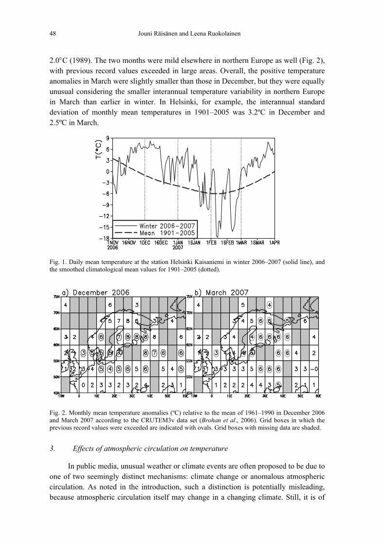
Even in the context of the large interannual and intraseasonal variability that is typical for winters in northern Europe, winter 2006�2007 was unusual. In Helsinki (Fig. 1), the first cold period occurred in the beginning of November, but it turned out to be short-lived. From mid-November to mid-December, daily mean temperatures remained remarkably steady around +6°C, a value typical for October. After this, the weather became somewhat more variable but mild conditions still dominated until 19 January. In contrast, the end of January and February were characterized by proper winter weather, including two decent cold-air outbreaks between a few short-lived thaws. However, the cold period terminated in the end of February, and March was mild from its very beginning, with gradually increasing temperatures towards the end of the month. On 26 March the maximum temperature in Helsinki reached 15.1°C, exceeding the previous March record of 12.6°C from 1945 by 2.5°C.

In terms of the monthly mean temperature, both December (4.0°C) and March (3.1°C) were warmer than ever before since the measurements in Helsinki commenced in 1829. The previous record value for December was 2.9°C (1929) and that for March


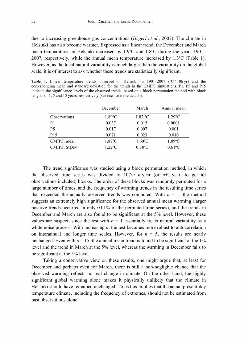
2.0°C (1989). The two months were mild elsewhere in northern Europe as well (Fig. 2), with previous record values exceeded in large areas. Overall, the positive temperature anomalies in March were slightly smaller than those in December, but they were equally unusual considering the smaller interannual temperature variability in northern Europe in March than earlier in winter. In Helsinki, for example, the interannual standard deviation of monthly mean temperatures in 1901�2005 was 3.2ºC in December and 2.5ºC in March.

Fig. 1. Daily mean temperature at the station Helsinki Kaisaniemi in winter 2006�2007 (solid line), and the smoothed climatological mean values for 1901�2005 (dotted).

Fig. 2. Monthly mean temperature anomalies (ºC) relative to the mean of 1961�1990 in December 2006 and March 2007 according to the CRUTEM3v data set (Brohan et al., 2006). Grid boxes in which the previous record values were exceeded are indicated with ovals. Grid boxes with missing data are shaded.

3. Effects of atmospheric circulation on temperature

In public media, unusual weather or climate events are often proposed to be due to one of two seemingly distinct mechanisms: climate change or anomalous atmospheric circulation. As noted in the introduction, such a distinction is potentially misleading, because atmospheric circulation itself may change in a changing climate. Still, it is of


interest to study how large a part of a given climatic anomaly can be explained by atmospheric circulation alone.

Here, we use the mean sea level pressure (MSLP) to explore the impact of atmospheric circulation on the temperatures observed in December 2006 and March 2007. As compared with circulation indicators for the free atmosphere, MSLP has the advantage that data are available for the whole 20th century. Here we use the HadSLP2 data set described by Allan and Ansell (2006).

In terms of the MSLP, December 2006 was a more anomalous month than March 2007. The north-south pressure gradient over northern Europe in December was exceptionally steep, with a quasi-permanent high over central and southern Europe and strong cyclone activity over the Norwegian and the Barents Seas (Figs. 3a�b). This resulted in unusually strong advection of mild air from the Atlantic Ocean into northern Europe. In March (Figs. 3c�d), the monthly mean MSLP field was closer to its long-term average. However, in this month as well, a negative pressure anomaly over the Arctic to the north of Scandinavia evidenced a northward shift in cyclone activity compared with average conditions. The monthly station-based North Atlantic Oscillation Index (NAOI) of Jones et al. (1997), which is commonly used for characterizing the atmospheric circulation over the North Atlantic and Europe, had in December 2006 its 4th highest December value (3.08) since 1901. NAOI for March 2007 (2.03) was also positive but far less extreme (21st highest since 1901).

Fig. 3. Mean sea level pressure (hPa) in December 2006 (a) and its deviation from the mean of 1901�2005 (b). (c)�(d) The same for March 2007. The five grid points used in the regression model of Section 3 are shown with closed circles.


To study in more quantitative terms, how large a part of the warm anomalies in Helsinki in December and March can be explained by the atmospheric circulation, a simple linear regression model was applied. The model used three candidate predictors, P, U and V, all computed from the monthly mean MSLP. P = MSLP(60°N, 25°E) represents the local pressure in southern Finland, whereas U = MSLP(55°N, 25°E) � MSLP(65°N, 25°E) and V = MSLP(60°N, 35°E) � MSLP(60°N, 15°E) are proxies for the west and the south components of the geostrophic wind, respectively. This model is chosen here for the simplicity of its physical interpretation, although it excludes the additional information potentially available in the MSLP field further away from southern Finland. More systematic approaches using, for example, the principal components of the MSLP field as predictors might be able to explain a somewhat larger fraction of interannual temperature variability than our regression model.

When testing the model in leave-one-out cross-verification over the period 1901�2005, the best predictions of temperature were obtained when using U and V as the predictors. In this case, the linear regression explained 62% of the temperature variance in December and 43% of the variance in March. The best one-predictor model (with U as the only predictor) explained 34% (35%) of the variance in December (March), whereas a linear model with all of P, U and V as predictors was marginally less skilfull than the two-predictor (U and V) model. Consequently, the model with U and V as the predictors was selected for further use.

Figure 4 shows scatter plots between the regression-predicted and observed temperatures. Unfortunately, although the model captures a substantial fraction of the interannual temperature variability particularly in December, the regression residuals are still large. The full range for December is from -6.3°C to 4.9°C and that for March from -5.7°C to 4.0°C. There are several potential reasons for this: the U and V predictors only carry a part of the information available in the monthly mean pressure field, the monthly mean pressure field itself gives an incomplete description of the actual variation of atmospheric circulation during the month, temperature might be affected by the snow and ice conditions preconditioned by the weather in the previous months, and so on.

For December 2006, the regression model predicts a mean temperature of 3.9ºC, which is 6.5ºC above the mean for 1901�2005 and only 0.1°C below the actually observed temperature. This is the highest December mean temperature predicted by the regression for any year since 1901 (Fig. 4a). The regression-predicted value for March 2007 is, however, only -0.6°C, or 1.8°C above the average for 1901�2005. This value is 3.7°C below the observed temperature, and it is by no mean exceptional when compared with the regression-predicted March mean temperatures in earlier years (Fig. 4b).

A naive interpretation of these results would be that (i) the mild temperatures in December 2006 were almost completely explained by an exceptional atmospheric circulation, whereas (ii) the circulation only explained a third of the warm anomaly in March 2007, leaving most of the anomaly to a circulation-independent contribution from global warming. However, the large interannual variability of the regression residuals in Fig. 4 clearly precludes such an exact deterministic interpretation.


Consequently, the potential �climate change contribution� in the positive temperature anomalies in these two months cannot be quantified with a sufficient accuracy by this method.

Fig. 4. Scatter plots between the temperatures predicted by the regression model of Section 3 and the temperatures observed in Helsinki in (a) December and (b) March. Later years are coded with increasingly dark shading, as indicated by the legend, and special symbols are used for December 2006 and March 2007.

Potentially, the performance of the regression model could be improved by a more

clever choice of the predictors. However, a rather large improvement would be required to make the results accurate enough. From model simulations, we would now expect the true climatological mean temperature in Helsinki in winter to be slightly over 1°C above its 20th century mean (Section 4). For the regression to reliably detect a climate change contribution of 1°C in the mean temperature of an individual month, the interannual standard deviation of the residuals should not be much larger than 0.5°C. This can be compared with the actual standard deviation of 1.9°C for both December and March in our regression model. To achieve this, the variance unexplained by the regression should be reduced by over an order of magnitude or, conversely, the explained variance should increase to about 97% in December and 96% in March. This is an extremely high accuracy requirement for any regression-based method.

4. Winter 2006�2007 in the context of the observed climate and estimated actual present-day climate

4.1 Analysis of observed trends

During the past century, the global mean temperature increased by 0.74 ± 0.18ºC (Trenberth et al., 2007), with most of the warming in the past 50 years being very likely


due to increasing greenhouse gas concentrations (Hegerl et al., 2007). The climate in Helsinki has also become warmer. Expressed as a linear trend, the December and March mean temperatures in Helsinki increased by 1.9ºC and 1.8ºC during the years 1901�2007, respectively, while the annual mean temperature increased by 1.3ºC (Table 1). However, as the local natural variability is much larger than the variability on the global scale, it is of interest to ask whether these trends are statistically significant.

Table 1. Linear temperature trends observed in Helsinki in 1901�2007 (ºC / 106 yr) and the corresponding mean and standard deviation for the trends in the CMIP3 simulations. P1, P5 and P15 indicate the significance levels of the observed trends, based on a block permutation method with block lengths of 1, 5 and 15 years, respectively (see text for more details).

December March Annual mean

Observations 1.89ºC 1.82 ºC 1.29ºC P1 0.037 0.015 0.0001 P5 0.017 0.007 0.001 P15 0.071 0.023 0.010 CMIP3, mean 1.87ºC 1.60ºC 1.09ºC CMIP3, StDev 1.22ºC 0.88ºC 0.61ºC

The trend significance was studied using a block permutation method, in which

the observed time series was divided to 107/n n-year (or n+1-year, to get all observations included) blocks. The order of these blocks was randomly permuted for a large number of times, and the frequency of warming trends in the resulting time series that exceeded the actually observed trends was computed. With n = 1, the method suggests an extremely high significance for the observed annual mean warming (larger positive trends occurred in only 0.01% of the permuted time series), and the trends in December and March are also found to be significant at the 5% level. However, these values are suspect, since the test with n = 1 essentially treats natural variability as a white noise process. With increasing n, the test becomes more robust to autocorrelation on interannual and longer time scales. However, for n = 5, the results are nearly unchanged. Even with n = 15, the annual mean trend is found to be significant at the 1% level and the trend in March at the 5% level, whereas the warming in December fails to be significant at the 5% level.

Taking a conservative view on these results, one might argue that, at least for December and perhaps even for March, there is still a non-negligble chance that the observed warming reflects no real change in climate. On the other hand, the highly significant global warming alone makes it physically unlikely that the climate in Helsinki should have remained unchanged. To us this implies that the actual present-day temperature climate, including the frequency of extremes, should not be estimated from past observations alone.


4.2 Model-based modification of observations

In RR08, a model-based approach for estimating the actual present-day temperature climate was proposed. In a hindcast test, which only used observations up to the year 1990, this technique was encouragingly successful in predicting the temperature climate that prevailed in land areas of the world during the period 1991�2002. Here, we apply this approach to December and March mean temperatures in Helsinki. We then proceed to estimate the return periods for the temperatures observed in December 2006 and March 2007, basing these estimates on one hand on the observed climate during the years 1901�2005 and on the other hand on the estimated present-day (early 21st century) climate.

To estimate the probability distributions that characterize present climate, a two-step procedure is followed. First, past observations are adjusted with the aim of making them representative of current climate conditions. Second, the desired probability distributions are derived from the distribution of these adjusted observations.

The adjustment is described in detail in RR08. Basically, the method assumes that the local time mean climate and the amplitude of interannual variability both change linearly with the 11-year running mean of the global mean temperature. The 11-year averaging is rather arbitrary, but is used as a simple way to filter out most of the unforced interannual variability in the global mean temperature. The evolution of the 11-year running mean global mean temperature is taken from observations (Brohan et al., 2006) up to the year 2002, after which is inferred from model simulations.

The regression coefficients that relate the local time mean climate and its interannual variability to the global mean temperature are purely model-based. They are derived from simulations spanning the 20th and 21st centuries, using the the Special Report on Emissions Scenarios (Naki�enovi� et al., 2000) A1B scenario for the latter. Because the simulations cover a longer period and a much larger range of global mean temperature change than the observations that are available to date, the regression coefficients derived from them are much less sensitive to sampling effects than would be the case for observation-based coefficients. Of course, this choice also includes a risk of bias, both because of model errors and because the patterns of forced climate change might change with time, for example due to changes in the balance between greenhouse gas and aerosol forcing. However, as we note below, the warming observed in Helsinki this far is consistent with the model simulations from which the regression coefficients are derived.

The adjustment is made separately for 22 coupled atmosphere-ocean general circulation models from 15 research institutions (Table 2), all participating in the World Climate Research Programme 3rd Coupled Model Intercomparison Project, CMIP3 (Meehl et al., 2007b). For comparison with the observed temperature trends shown in the top of Table 1, the mean and inter-model standard deviation of the simulated temperature trends in the grid box closest to Helsinki are shown in the bottom of the same table. While the observed warming in 1901�2007 was slightly larger than the


warming on the average simulated by the models, particularly in March, the difference is small and well within the variability between the individual models.

Table 2. The CMIP3 models used in this study.

Model Institution

BCCR-BCM2.0 Bjerknes Centre for Climate Research, Norway

CGCM3.1 (T47) Canadian Centre for Climate Modelling and Analysis

CGCM3.1 (T63) same as previous

CNRM-CM3 Météo-France

CSIRO-MK3.0 CSIRO Atmospheric Research, Australia

ECHAM5/MPI-OM Max Planck Institute (MPI) for Meteorology, Germany

ECHO-G University of Bonn and Model & Data Group, Germany; Korean Meteorological Agency

FGOALS-g1.0 Chinese Academy of Sciences

GFDL-CM2.0 Geophysical Fluid Dynamics Laboratory, USA

GFDL-CM2.1 same as previous

GISS-AOM Goddard Institute for Space Studies, USA

GISS-EH same as previous

GISS-ER same as previous

INM-CM3.0 Institute for Numerical Mathematics, Russia

IPSL-CM4 Institut Pierre Simon Laplace, France

MIROC3.2 (hires) Center for Climate System Research, National Institute for Enviromental Studies and Frontier Research Center for Global Change, Japan

MIROC3 (medres) same as previous

MRI-CGCM2.3.2 Meteorological Research Institute, Japan

NCAR-CCSM3 National Center for Atmospheric Research, USA

NCAR-PCM same as previous

UKMO-HadCM3 Hadley Centre for Climate Prediction and Research / Met Office, UK UKMO-HadGEM same as previous

The adjustment of the December and March mean temperatures in Helsinki is

illustrated in Fig. 5. As a result of the intermodel variation in the regression coefficients (and, to a smaller extent, in the global warming simulated after 2002), 22 estimates of the �equivalent� present-day temperature are obtained for each past temperature observation. However, for both December and March and for all 22 models, the adjusted temperatures exceed the observed values for all years in 1901�2005. The difference increases backwards in time, because the global mean temperature was further below its present-day level in the early 20th century than in the last few decades.


For the same reason, the scatter among the 22 estimates also increases backwards in time. Finally, one may note that the adjustment increment to the observed temperatures tends to be slightly larger for cold than mild December and March months. This is because, in both December and March, most of the models suggest a decrease in interannual temperature variability in southern Finland with increasing global mean temperature. On the average, the models suggest a 2.1°C (1.8°C) increase in the local December (March) mean temperature in Helsinki, and an 8% (9%) decrease in the interannual standard deviation, for each 1°C of global mean warming.

Fig. 5. Observed (a) December and (b) March mean temperatures in Helsinki in 1901�2005 (solid line), and the adjusted monthly mean temperatures based on the method described in Section 4. The small grey dots show the temperatures based on the results of the 22 individual models and the larger dots the 22-model mean.

4.3 Return period estimates

We now proceed to estimate the probability of occurrence of extremely warm months (i.e., equal to or warmer than a selected threshold value) and the equivalent return periods (inverse of the exceedance probability). In doing this, two partly subjective choices are needed: weighting between the probabilities based on the results of the 22 models, and the way in which probability is estimated from a single time series of 105 (original or adjusted) observations. As for the weighting, we simply assume that all 22 models give equally plausible results and therefore deserve the same weight, but we also study the range of return periods obtained from the individual models.

For converting a time series of observations to a probability estimate, a raw count of cases that exceed the selected temperature threshold is one option. However, this method gives no meaningful information on the exceedance probability of temperatures outside the range of values that actually occur in the time series. For this extrapolation to the extreme tails, and also for reducing the sampling variability of the probability estimates in the inner parts of the distribution, analytical functions fitted to the data can be used. Unfortunately, the fitting might also introduce systematic errors, if the actual and the assumed form of the distribution differ.


As a first choice, the Generalized Pareto Distribution (GPD) as implemented in the Extremes Toolkit developed at the United States National Center of Atmospheric Research (Gilleland et al., 2005; Katz et al., 2005) was tested. However, the results appeared problematic. For the December and March mean temperatures observed in 2006�2007, infinite return period estimates were obtained. Furthermore, the method suggested a return period of 350 (500) years for the warmest December (March) mean temperature observed in 1901�2005, i.e. 2.9ºC (2.0ºC). These return periods seem surprisingly long, particularly as these peak values were not outliers when compared with the other December and March mean temperatures in 1901�2005 (the second highest value for December being 2.8ºC and that for March 1.8ºC). This apparent mismatch suggests that the assumptions underlying the GPD distribution or their specific implementation in the Extremes Toolkit may not be well fulfilled by our temperature data.

Consequently, we reverted to the Gaussian kernel smoothing used in RR08. The probability density f(T) is calculated as

�=

=��

��

�−−

−+−=

Ni

ii bsMTb

N

NMTG

NbsTf

1

2 /)))()1(1

((1

)( (1)

where, in the present application, N = 105. Ti (1 � i � N) are the observed or adjusted temperatures in the years 1901�2005, and M and s are their mean and standard deviation. b (0 < b � 1) is a smoothing coefficient and G is the density function of the standard normal distribution. For b = 1, (1) returns a Gaussian distribution with mean M and standard deviation s. For smaller values of b, the mean and the standard deviation are the same, but the shape of the distribution follows the original discrete distribution more closely. With increasing b, sampling errors in the density function f(T) and in the cumulative distribution function decrease. On the other hand, too strong smoothing may introduce systematic biases in the smoothed distribution, particularly near its tails, if the distribution of the input data differs significantly from normal. There is thus a trade-off between these two factors, but the exact choice of b is unfortunately quite subjective.

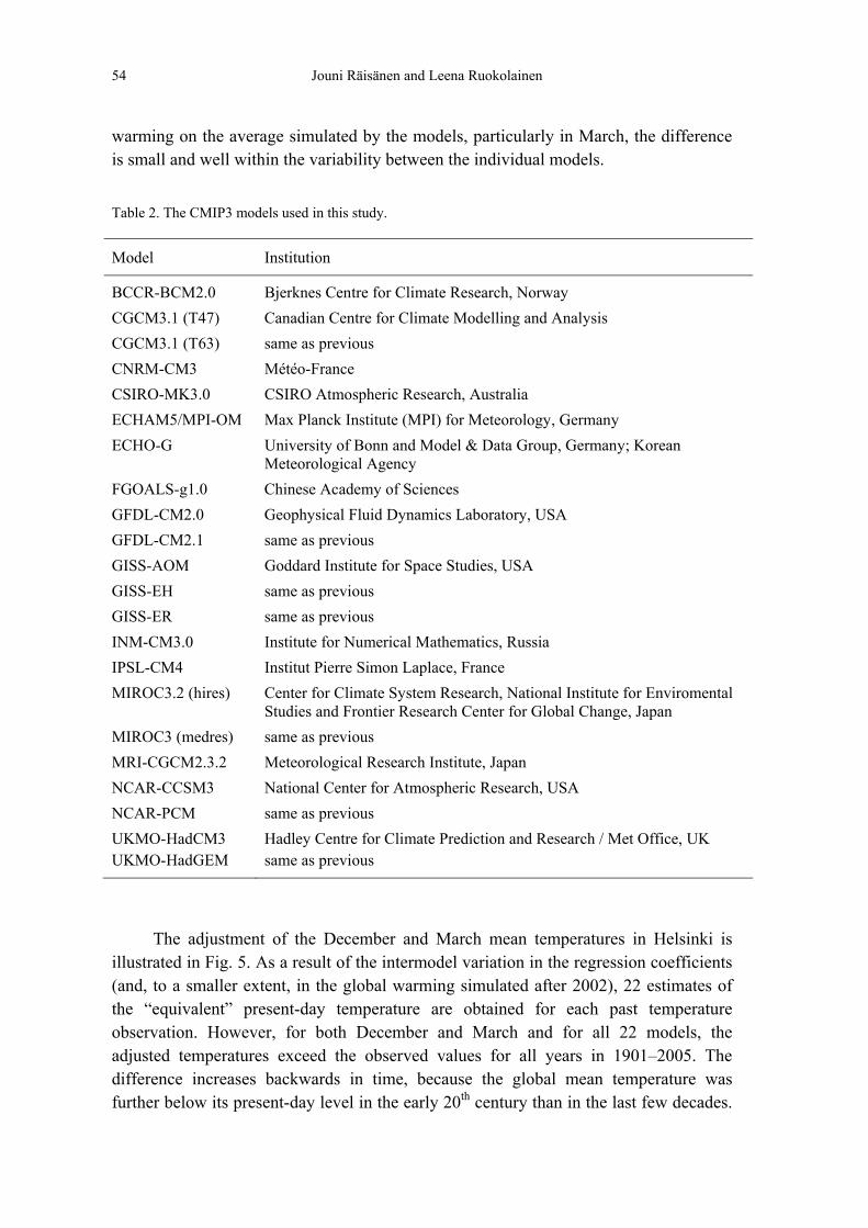
Figure 6a compares the observed (1901�2005) frequency distribution of December mean temperature with the continuous distributions obtained with four values of b (1, 1/2, 1/3, and 1/5). The observed distribution is substantially skewed, with a long tail to the left. The coefficient of skewness is -0.71, being significantly different from zero at the 0.5% risk level. As a result, the pure normal distribution (b = 1) fits the data badly, giving spuriously high probabilities for very mild December mean temperatures. With decreasing b, the agreement with the observed distribution improves. On the other hand, with the lowest of the tested values (b = 1/5), the continuous distribution clearly begins to pick up such irregularities of the observed distribution that most likely result from sampling variability.

The probability estimates in the extreme upper tail are very sensitive to the choice of b (Fig. 6b). The resulting return period estimates for TDecember � 4.0ºC are only 54 years for b = 1 and 145 years for b = 1/2, but the poor fit to the actual data makes such


short return periods appear unlikely. For, b = 1/3, a return period of 340 year is obtained, whereas b = 1/5 increases the return period to 1700 years.

For the rest of the paper, we use the value b = 1/3 for both December and March, but we stress that this choice is subjective. However, as shown in the Appendix, the return period estimates that are obtained with b = 1/3 agree within a factor of two with a very different method based on Monte Carlo sampling of daily temperature observations. This gives us some confidence that our choice of b is reasonable for the present purpose.

Fig. 6. (a) Frequency distribution of observed December mean temperatures in Helsinki in 1901�2005 (bars) and the continuous probability distribution estimated with the Gaussian kernel, for four values of the smoothing coefficient b (see the legend for explanation of line types). (b) The same for the cumulative probability function under the temperature range 1�5ºC. The bold step line represents the discrete distribution obtained directly from the observations and the four smooth lines the distributions from the Gaussian smoothing.

The probability density functions of December and March mean temperature obtained with b = 1/3 are shown in Fig. 7. In December, there is a warming of about 1.3ºC in the mean value between the distribution representing the observed (1901�2005) climate and the multi-model mean estimate of the present climate, whereas the corresponding warming in March is 1.1ºC. However, due to the decrease in interannual variability in most of the models, the shift in the upper tail of the distribution is slightly smaller. Although the results based on the 22 individual models vary, all the models indicate a substantial increase in the probability of very high December and March mean temperatures.


Fig. 7. (a) Probability distributions of (a) December and (b) March mean temperature in Helsinki, using Gaussian kernel smoothing with b = 1/3. The dashed line shows the observed distribution for 1901�2005, and the other lines model-based distributions corresponding to the climate in 2006�2007 (thin lines for the individual 22 models and lines with open circles for the 22-model mean).

The probability of exceeding the temperatures observed in winter 2006�2007 can be visually evaluated from Fig. 7 as the area below the probability curves and to the right of the vertical lines at 4.0ºC (December) and 3.1ºC (March). The resulting return period estimates are given in Table 3, both for these thresholds and for the previous record values of 2.9ºC in December and 2.0ºC in March. Despite the uncertainties associated with both the curve fitting and the differences between the climate change estimates from the 22 models, the results suggest that the probability of extremely mild winter months is now much larger than the observations for 1901�2005 would indicate. The resulting best-estimate return period for TDecember � 4.0ºC, 57 years, is six times shorter than the value of 340 years derived directly from the observations, and the corresponding difference for TMarch � 3.1ºC (84 versus 725 years) exceeds a factor of eight. Even for the models with the smallest warming, and therefore the smallest shift in the probability distributions, the decrease in these two return periods is about a factor of three. Furthermore, a large decrease in return periods is also found for the temperature thresholds that correspond to the previous record values. Our best-estimate present-day return period for TDecember � 2.9ºC, 17 years, is less than a third of the value derived from past observations. Similarly, a March mean temperature of at least 2.0ºC is now estimated to occur in one year out of 14, which is four times more often than the corresponding Gaussian kernel estimate for 1901�2005. Furthermore, because the last several decades of the period 1901�2005 were already non-negligibly affected by anthropogenic global warming, the difference in return periods between the present and the truly preindustrial climate would be even larger.

For comparison, the adjustment of past temperature observations was repeated without including changes in interannual variability. Because the variability decreases in most models, the neglect of this leads to a larger shift in the upper end of the temperature distribution. Thus, shorter present-day return period estimates for high


temperatures are obtained, although the difference is relatively modest (compare the last and second rows of Table 3).

Table 3. Estimated return periods (years) for December and March mean temperature in Helsinki. The thresholds 2.9ºC and 2.0ºC are the warmest December and March mean temperatures prior to the year 2006, whereas 4.0ºC and 3.1ºC are the corresponding values for winter 2006�2007. In each table cell, the first value is based on Gaussian kernel smoothing with b = 1/3, and the second value on a direct count of cases (--- where the threshold value exceeds the maximum of the data set). The estimates for winter 2006�2007 are based on the method detailed in Section 4.2. The best estimate, minimum and the maximum are derived from the corresponding 22-model mean probability estimates and the intermodel range of these estimates.

December March

� 2.9ºC � 4.0ºC � 2.0ºC � 3.1ºC

1901�2005, observations 56 (105) 340 (---) 57 (105) 725 (---)

2006�2007, best estimate 17 (18) 57 (96) 14 (12) 84 (2310)

2006�2007, minimum 10 (11) 28 (35) 9 (8) 33 (105)

2006�2007, maximum 26 (26) 122 (---) 25 (53) 221 (---)

2006�2007, best estimate with unchanged variability

14 (15) 41 (51) 10 (11) 51 (257)

As an additional check, we recalculated the return periods from the exceedance probabilities obtained from a simple count of cases. The results for this alternative, which avoids the potential systematic biases of analytical distributions but is prone to larger sampling errors, are shown in parentheses in Table 3. When applied to the observations from 1901�2005, the direct count gives no meaningful information on the return period of the temperatures observed in December 2006 and March 2007, and a return period of 105 years for the previous record values of 2.9ºC in December and 2.0ºC in March. For the present-day climate, the return period estimates for these 2.9ºC and 2.0ºC thresholds are very similar to those obtained from the Gaussian kernel. For the 4.0ºC (December) and 3.1ºC (March) thresholds, larger differences occur, the direct count giving longer return periods than the Gaussian kernel. This might suggest that the Gaussian kernel gives too short return periods for extremely warm temperatures, but this suggestion must be weighted against the large sampling errors in the tail of the distribution. The most striking case of apparent disagreement occurs for TMarch � 3.1ºC, the direct count suggesting a present-day return period of 2310 years and the Gaussian kernel 84 years. Yet, when the threshold is lowered by just 0.4ºC to 2.7ºC, the return period estimate from the direct count method decreases to 92 years. Thus, the difference between the methods is much less dramatic in terms of temperature than in terms of the return period.

Finally, return period is a potentially misleading term in a changing climate. If climate changes proceed as suggested by the model simulations for the A1B scenario, the winter mean temperature in Helsinki should increase by about 2ºC from its present-


day (2008) level by the year 2050. As a result of this warming, the probability of very high December and March mean temperatures is likely to increase rapidly with time. For threshold values that just exceed the new records from winter 2006�2007 (4.1ºC in December and 3.2ºC in March), the multi-model mean results suggest a yearly probability of occurrence of over 4% in the year 2030 and almost 14% in 2050 (Fig. 8a). The record values from winter 2006�2007 are therefore unlikely to survive as long as their present-day return periods suggest. For both December and March, there appears to be about a 50% probability that new records will be set within the next 25 years, and about a 90% probability that this will happen by the year 2050 (Fig. 8b)1. These results should be nearly independent of the choice among the SRES scenarios, which, however, would become important in the second half of the 21st century (Meehl et al., 2007a).

Fig. 8. (a) Estimated probabilities for the March (solid line) and December (dashed line) mean temperatures in Helsinki exceeding the values observed in winter 2006�2007. (b) The corresponding cumulative probabilities, assuming that the temperatures in consecutive years are uncorrelated. The figure is based on all-model mean probabilities for the A1B emissions scenario, using Gaussian kernel smoothing with b = 1/3.

5. Summary

An increase in the magnitude and frequency of warm extremes is regarded as a very likely consequence of projected future global warming (Meehl et al., 2007a), and some evidence for such an increase is already seen in observations (Trenberth et al., 2007). Yet, the interpretation of any single extreme event is a challenge, not least for the operational meteorologists that are approached from the media with the inherently unfair question of �was this caused by climate change�?

Here, we have studied the interpretation of two record warm winter months in Helsinki, Finland, December 2006 and March 2007, by using observations and model simulations. First, a regression model was built to study the connection between the observed temperatures and the atmospheric circulation. This model suggested that almost the whole warm anomaly in December was due to exceptionally strong westerly

1 If the direct count method had been used instead of the Gaussian kernel, the time of crossing the 50% level in Fig. 8b would have been delayed by 3�5 years. Conversely, if the observations from winter 2006�2007 had been included in the calculation, this time would have been advanced by 2�4 years.


flow from the North Atlantic into northern Europe, but it only attributed a third of the temperature anomaly in March to anomalous circulation. These results might seem to suggest a substantial �climate change component� in the warmth of March but not in December, but such a clear-cut interpretation is unwarranted.

The first and most important difficulty relates to the imperfect skill of the regression model. Because the interannual variability of the regression residuals was much larger than the likely magnitude of the actual �climate change component� in the observed temperatures, it is obvious that the latter cannot be meaningfully estimated from the regression results. While a more skillful regression model might reduce this problem to some extent, a very large improvement would have been required to achieve sufficient accuracy. This problem in the interpretation of regression results is likely to be pertinent to all areas with large interannual climate variability.

As a second complication, the atmospheric circulation itself might change with changing climate. In fact, an increase in wintertime westerlies in northern Europe is a common feature in, at least, most climate model simulations with increased greenhouse gas concentrations (Meehl et al., 2007a). Yet, because this change in circulation is too small to be the dominant cause of the warming in climate models (Rauthe and Paeth, 2004; Stephenson et al., 2006), this issue is probably less important than the inherent statistical uncertainty in the regression residuals.

Second, we used a frequentist approach. The probability of temperatures similar to or higher than those observed in December 2006 and March 2007 was first estimated by fitting analytical distributions to the observations from 1901�2005. Then, the same calculation was repeated after adjusting the observations for climate change, by using the observed evolution of the global mean temperature and results from 22 climate models.

Although the quantitative probability estimates obtained from this calculation were sensitive to the details of curve fitting, the general conclusions were very clear. As estimated from the observed variation of temperature in 1901�2005, the temperatures that occurred in December 2006 and March 2007 were found to have a return period of several hundred years. After the model-based adjustment of the observations for climate change, however, best-estimate return periods of less than a century were obtained. Even when the models with the smallest warming in southern Finland were used for deriving the adjustments, the present-day return periods were still found to be a factor of three shorter than the return periods estimated from the previously observed climate. Thus, although it is impossible to prove a causal connection between the ongoing global warming and the warmth of December 2006 and March 2007 in Helsinki, our analysis suggests that the probability of occurrence of such extremely mild months has already been substantially increased from what it was before.

Even for the estimated present-day climate conditions, the warmth of December 2006 and March 2007 appears fairly unusual. However, it is essential to remember the selection effect: these two months were chosen for this study just because they were exceptional. In Helsinki, no other record warm months occurred during the first seven


years of the 21st century. Observing two very warm months with a return period of 50�100 years during a seven-year period is by no means statistically unusual.

Finally, the return period estimates derived for the present climate will not be representative for the future. Our analysis of model simulations for the A1B scenario suggests about a 90% probability that the records from December 2006 and March 2007 will be broken at least once by the year 2050.

Acknowledgments

We acknowledge the modeling groups for making their model output available as part of the WCRP's CMIP3 multi-model dataset, the Program for Climate Model Diagnosis and Intercomparison (PCMDI) for collecting and archiving this data, and the WCRP's Working Group on Coupled Modelling (WGCM) for organizing the model data analysis activity. The WCRP CMIP3 multi-model dataset is supported by the Office of Science, U.S. Department of Energy. We also thank Mr. Seppo Saku for making the calculations with the extRemes software, and the two referees for their constructive comments. This research has been supported by the Academy of Finland (decision 106979) and by the ACCLIM project within the Finnish Climate Change Adaptation Research Programme ISTO.

References

Allan, R.J. and T.J. Ansell, 2006. A new globally complete monthly historical mean sea level pressure data set (HadSLP2): 1850�2004. J. Climate, 19, 5816�5842.

Allen, M., 2003. Liability for climate change. Nature, 421, 891�892. Black E., M. Blackburn, G. Harrison, B. Hoskins and J. Methven, 2004. Factors

contributing to the summer 2003 European heatwave. Weather, 59, 217�223. Brohan, P., J.J. Kennedy, I. Harris, S.F.B. Tett and P.D. Jones, 2006. Uncertainty

estimates in regional and global observed temperature changes: a new dataset from 1850. J. Geophys Res, 111, D12106, doi:10.1029/2005JD006548.

Fink, A.H., T. Brücher, A. Krüger, G.C. Leckebusch, J.G. Pinto and U. Ulbrich, 2004. The 2003 European summer heatwaves and drought � synoptic diagnosis and impacts. Weather, 59, 209�216.

Gilleland, E., R. Katz and G. Young, 2005. Extremes toolkit (extRemes): Weather and climate applications of extreme value statistics. http://www.assessment.ucar.edu/ toolkit/.

Hegerl, G.C. and co-authors, 2007. Understanding and Attributing Climate Change. In: Climate Change 2007: the Physical Science Basis (eds. S. Solomon, D. Qin, M. Manning, M. Marquis, K. Averyt, M.M.B. Tignor, H. LeRoy Miller, Jr. and Z. Chen) Cambridge University Press, Cambridge, United Kingdom and New York, NY, USA, pp 663�745.


Jones, P.D., T. Jónsson and D. Wheeler, 1997. Extension to the North Atlantic Oscillation using early instrumental pressure observations from Gibraltar and South-West Iceland. Int. J. Climatol., 17, 1433�1450.

Katz, R. W., G.S. Bruzh and M. Parlange, 2005. Statistics of extremes: modelling ecological disturbances. Ecology, 86, 1124�1134.

Kharin, V.V., F.W. Zwiers, X. Zhang and G.C. Hegerl, 2007. Changes in temperature and precipitation extremes in the IPCC ensemble of global coupled model simulations. J. Climate, 20, 1419�1444.

Meehl, G.A. and C. Tebaldi, 2004. More intense, more frequent and longer lasting heat waves in the 21st century. Science, 305, 994�997.

Meehl G.A. and co-authors, 2007a. Global climate projections. In: Climate Change 2007: the Physical Science Basis (eds. S. Solomon, D. Qin, M. Manning, M. Marquis, K. Averyt, M.M.B. Tignor, H. LeRoy Miller, Jr. and Z. Chen) Cambridge University Press, Cambridge, United Kingdom and New York, NY, USA, pp 747�845.

Meehl G.A. and co-authors, 2007b. The WCRP CMIP3 Multimodel Dataset: A New Era in Climate Change Research. Bull Am Meteor Soc 88, 1383�1394.

Naki�enovi� N. and co-authors, 2000. Emissions Scenarios. A Special Report of Working Group III of the Intergovernmental Panel on Climate Change. Cambridge University Press, Cambridge, United Kingdom and New York, NY, USA, 599 pp.

Räisänen, J. and L. Ruokolainen, 2008. Estimating present climate in a warming world: a model-based approach. Climate Dyn., 31, 573�585.

Rauthe, M. and H. Paeth, 2004. Relative importance of Northern Hemisphere circulation modes in predicting regional climate change. J. Climate, 17, 4180�4189.

Sheffield, J. and E.F. Wood, 2008. Projected changes in drought occurrence under future global warming from multi-model, multi-scenario, IPCC AR4 simulations. Climate Dyn., 31, 79�105.

Stephenson, D.B., V. Pavan, M. Collins, M.M. Junge, R. Quadrelli and Participating CMIP2 Modelling Groups, 2006: North Atlantic Oscillation response to transient greenhouse gas forcing and the impact on European winter climate: a CMIP2 multi-model assessment. Climate Dyn., 27, 401�420.

Stott, P.A., A.D. Stone and M.R. Allen, 2004. Human contribution to the European heatwave of 2003. Nature, 432, 610�614.

Trenberth, K.E. and co-authors, 2007. Observations: Surface and Atmospheric Climate change. In: Climate Change 2007: the Physical Science Basis (eds. S. Solomon, D. Qin, M. Manning, M. Marquis, K. Averyt, M.M.B. Tignor, H. LeRoy Miller, Jr. and Z. Chen) Cambridge University Press, Cambridge, United Kingdom and New York, NY, USA, pp 235�336.


Appendix: estimation of the probability distribution on monthly mean temperatures from daily temperature data

This appendix describes a simple method for estimating the probability distribution of monthly mean temperatures from daily temperature data. This method is not applicable to our estimates of actual present-day climate, because the technique developed in RR08 has not yet been extended to the modification of daily temperature observations. However, the method provides an alternative means of estimating the baseline temperature climate in the years 1901�2005. The method consists of the following eight steps:

1. Calculate, for the given calendar month, the long-term mean (Mmon) and variance (Vmon) of the monthly mean temperature.

2. Calculate, separately for each calendar day, the long-term mean of the daily mean temperature. Then compute, for each day in the time series, the daily temperature anomaly by subtracting the long-term daily mean from the observed value.

3. Compute, for each calendar day, the mean square of the daily temperature anomalies. Denote the average of this over the whole calendar month as Sday.

4. Calculate the ratio R = Sday / Vmon. Denote the integer part of this as IR.

5. Select, by random, IR+1 daily temperature anomalies from the daily anomalies available for the given calendar month.

6. Calculate a weighted mean of the selected anomalies. The first IR anomalies are given unit weight, whereas the last is given a lower weight of

( )

1

1

−

−+⋅−=

R

RIRIRRIRw (A1)

7. Add the weighted mean anomaly obtained from step 6 to the long-term mean monthly mean temperature Mmon. Denote the result as Tsim.

8. Repeat the steps 5�7 a large number (here: one million) of times to estimate the probability distribution of Tsim.

By this procedure, the mean of Tsim becomes Mmon. Furthermore, with the weights chosen in step 6, the variance of Tsim becomes (from the additivity of variances applied to a weighted sum)

MonDay

DayDay

sim VR

S

wIR

wS

wIR

SIRTV ==�

��

��

++

+=

2

2)()( (A2)

For R > 2 there would be alternative ways of choosing the weights that would give the same variance, but the one specified in step 6 is the simplest. The ratio R tells, in essence, how many �independent� days there are in terms of temperature in a given


month. For the observations in Helsinki in 1901�2005, RDecember = 2.99 and RMarch = 2.75. Thus, in these months, the characteristic time scale of temperature variation in Helsinki is of the order of ten days.

Except for Mmon and Vmon, this Monte Carlo simulation procedure includes no information on the observed frequency distribution of monthly mean temperatures. Nevertheless, the resulting distributions of Tsim replicate the general shape of these observed distributions remarkably well, and they are in even closer agreement with the Gaussian kernel estimate with b = 1/3 (Figure A1). This suggests that the observed skewness of the monthly mean temperature distributions, with a long tail to the left, is a direct consequence of a similar (but stronger) skewness in the distribution of daily temperatures.

Fig. A1. (a) Frequency distribution of observed December mean temperatures in Helsinki in 1901�2005 (bars) and the continuous probability distributions estimated by Monte Carlo simulation based on daily data (solid line) and with the Gaussian kernel with b = 1/3 (dashed line). (b) as (a), but for March.

For both December and March, the good agreement between the two methods extends even to the extreme right tail. The resulting best-estimate return period for TDecember � 4.0ºC from the simulation method is 608 years, to be compared with 340 years from the Gaussian kernel. For TMarch � 3.1ºC, the simulation method suggests a return period of 441 years, whereas the Gaussian kernel gives 725 years. Although this broad agreement is no absolute proof of correctness, it supports the idea that the estimated return periods of several hundred years are of the right order of magnitude.

Ongoing Global Warming and Local Warm Extremes: a Case ... · Ongoing Global Warming and Local Warm...

Documents

Transcript of Ongoing Global Warming and Local Warm Extremes: a Case ... · Ongoing Global Warming and Local Warm...