One-Sample Proportions

Chapter 2

One-Sample Proportions

2.1 Introduction: Qualitative Data

The simplest types of measurements are qualitative in nature, meaning thatthey are non-numeric – or at least numeric manipulation of them is mean-ingless – and include names, labels and group membership. Examples ofqualitative data are ubiquitous, but are best exemplified by dichotomouscategorical data consisting of only two possible values, such as a patient’sgender (male or female), diagnosis of a certain disease (positive or negative),or the result from a health intervention (success or failure).

Dichotomous categorical data are typically described in terms of the pro-portion (p) of some population with one of the two possible characteristics.This value is defined as the total number of subjects in some populationexhibiting that specific characteristic divided by the number of total subjects(N) in that population. For instance, if 105 out of 200 physicians in a givenhospital are female, then the proportion of these physicians who are female ispf = 105/200 = 0.525. It should stand to reason that a proportion can onlytake values between 0 and 1.0, as you cannot have fewer than zero subjectswith a given characteristic (reflecting p = 0/N = 0), just as you cannot havemore than the total number subjects with a given characteristic (reflectingp = N/N = 1.0).

The Complement Rule: The outcomes for dichotomous data must also bemutually exclusive, in the sense that any given subject may assume only oneof the two potential outcomes at one time. For instance, a subject cannotsimultaneously test positive and negative for a disease. In general we willignore instances where the outcomes are not mutually exclusive; in practice itis best to avoid these scenarios all together. One benefit of this characteristicis that we only need to know the proportion of one of the two outcomes toknow the proportion for both. Returning to our previous example, if thereare 105 female physicians, then there must be 200−105 = 95 male physicians,meaning the proportion of male physicians is pm = 95/200 = 0.475. Note here

R. Sabo and E. Boone, Statistical Research Methods: A Guide forNon-Statisticians, DOI 10.1007/978-1-4614-8708-1 2,© Springer Science+Business Media New York 2013

13

14 CHAPTER 2. ONE-SAMPLE PROPORTIONS

that there are 105 + 95 = 200 physicians who are either male or female,meaning that the proportion of physicians who are either male or female ispe = 200/200 = 1.0. Further, note that pf + pm = 0.525 + 0.475 = 1.0 = pe.This will always be the case for dichotomous categorical data. So if we knowthat pf = 0.525, then we can use what is called the complement rule to findpm = 1− pf = 1− 0.525 = 0.475.

As a final note on proportions, there is a one-to-one relationship betweenproportions and percentages, meaning that for every proportion between 0and 1.0, there is a corresponding percentage between 0 and 100%. This meansthat we should be able to transform proportions into percentages – and per-centages into proportions – with ease. Without getting into the mathematicalrationale, the algorithm is simple: to turn a proportion into a percentage,move the decimal two places to the right and add a percent sign (%). Forexample, if we have the proportion p = 0.525, we turn it into the percent-age 52.5%. Likewise, if we have a percentage (say 47.5%), we turn it into aproportion by moving the decimal two places to the left and removing thepercent sign (0.475).

2.2 Establishing Hypotheses

The key problem here is that we generally do not know the exact valueof a population proportion, and at times we might not even know the totalnumber of subjects comprising that population. This is problematic for thosewho may want to base their decisions or actions on such a proportion. Forinstance, in deciding between two different treatments to administer to apatient, a physician might want to know the success rates – read: propor-tions – of those two treatments before choosing between them. These pop-ulation values are rarely known, but certainly the physician – or others in asimilar situation – must make a decision, so something else must be done.

Thus enters the statistical method and the formation of a hypothesis.When a population proportion is unknown, we must formulate competingand mutually exclusive hypotheses about that proportion, collect data repre-sentative of the desired population, evaluate that data, and determine whichhypothesis the evidence supports. The first step in this process is to set upcompeting hypotheses to test. There is generally some hypothesized value(p0 – pronounced “p-naught”) in which we are interested; for instance, maybeit is commonly accepted that the success-rate of a given treatment is 0.5(treatment is successful for half of all patients and unsuccessful for the otherhalf). This value then becomes the central crux around which we form ourhypotheses.

As mentioned in Chapter 1, we will create two mutually exclusive hyp-otheses, such that only one can be true at a time. We name these hypothesesthe null and alternative hypotheses, and we have a formal process fordetermining which hypothesis gets which name (the naming procedure isactually important). The null hypothesis (H0) is that hypothesis which states

2.3. SUMMARIZING CATEGORICAL DATA (WITH R CODE) 15

our parameter is equal to some value (p0), while the alternative hypothesis(HA) indicates that the parameter is somehow different from p0. Depend-ing upon our research question, there are three possible ways in which theparameter – proportion in this case – can differ from p0: it can be less thanp0 (represented by the symbol <), it can be greater than p0 (represented bythe symbol >), or it can be not equal to p0 (represented by the symbol �=).To choose between these three options we begin by translating our researchquestion into symbolic form, which will include one of the following options:<, ≤, >, ≥, = or �=. As an example, suppose our research question is thatthe proportion of subjects with adverse toxic reactions to a particular drugis less than 0.3. In order to turn this into a symbolic statement, we mustidentify the operative phrase “is less than”, which is stating that p < 0.3.

The second step is to find the functional opposite of the statement fromour research question. Based on the symbolic form from our research ques-tion, we create the functional opposite by pairing the following symbols:(< and ≥), (> and ≤) or ( = and �=). Note that each of these pairs compriseall possibilities for a given situation (e.g. you are either strictly less thansome value or greater than or equal to some value; either greater than somevalue or less than or equal to some value; either equal to some value or notequal to some value). Returning to our example, the functional opposite ofthe symbolic form of our research question (p < 0.3) is p ≥ 0.3.

The third step is to identify which of our two symbolic forms is the nullhypothesis and which is the alternative hypothesis, which is easier to do thanto explain. Of the two symbolic forms, the form with some equality (meaningthe =, ≤ or ≥ signs) becomes the null hypothesis, while the symbolic formwithout any equality (meaning the �=, < or > signs) becomes the alternativehypothesis. Further, regardless of the symbol in the statement that belongsto the null hypothesis, we use the = sign. (We do this for practical reasons,as we’re going to assume the null hypothesis is true, and doing so is mucheasier if H0 contains only one value rather than a range of values. Keepin mind, however, that this practical reason is not the same as theoreticaljustification, which will be given elsewhere.) For our example, the statementp ≥ 0.3 contains equality, while the statement p < 0.3 does not. So our alter-native hypothesis becomes HA : p < 0.3, while the null hypothesis becomesH0 : p = 0.3. This process can be followed for most research statements con-cerning one population proportion, and Table 2.1 lists the possible hypothesesas well as key words to help in guiding you to the appropriate pair.

2.3 Summarizing Categorical Data

(with R Code)

Sample Proportion: Given a set of hypotheses about a population proportion,the next step is to collect evidence that will (hopefully) support one of thetwo hypotheses. When we are interested in a population proportion, the


Table 2.1: Possible Sets of Hypotheses for a Population Proportion BasedUpon Key Phrases in a Research Question.

Key Phrases“less than” “greater than” “equal to”

“greater than or equal to” “less than or equal to” “not equal to”Hypothesis “at least” “at most”

Null H0 : p = p0 H0 : p = p0 H0 : p = p0Alternative HA : p < p0 HA : p > p0 HA : p �= p0

logical step would be to calculate a sample proportion from a representativesample drawn from the population of interest. The sample proportion p̂serves as an estimate of the population proportion, and is calculated in asimilar manner as its population analogue, being the number of subjects xin a sample exhibiting a particular characteristic (often referred to as thefrequency) divided by the total number of subjects n in the sample (referredto as the sample size). So if we have a random sample of 25 physicians,13 of whom are female, then the proportion of female physicians in thissample is p̂f = 13/25 = 0.52. Due to the dichotomous nature of this type ofmeasurement, we can use the complement rule to find the sample proportionof male physicians (p̂m = 1− 0.52 = 0.48).

Rounding: Depending on the sample size, you will have different rules forrounding proportions. For sample sizes greater than 100, round p̂ to at mostthree decimal places (e.g. p̂ = 0.452). For sample sizes less than 100 butgreater than 20, round p̂ to two decimal places (e.g. p̂ = 0.45). For smallsample sizes less than ∼20, the ratio of frequency to sample size should bereported as a fraction (x/n) (e.g. 5/11) and the sample proportion shouldnot be calculated (note that there is no universally agreed upon value for thislast rule, and 20 was selected for presentation).

2.4 Assessing Assumptions

If our random sample is adequately representative of the parent populationfrom which it is drawn, then our sample estimate p̂ should be close to the pop-ulation value p. Unless we have clear evidence or information to the contrary,we will assume: (i) that the sample used to calculate p̂ is representative, and(ii) that the subjects in the sample from whom measurements were takenare independent of one another. To determine if the sample is of sufficientsize, we need to check the following conditions: based on the condition setforth in the null hypothesis H0, we need to expect there to be at least fivesubjects taking either value of the categorical variable. This expectation isdetermined by noting that if the proportion of subjects taking the first cate-gory is p0 = 0.3 according to H0 (meaning the proportion taking the second

2.5. HYPOTHESIS TEST FOR COMPARING A POPULATION. . . 17

category is q0 = 1 − p0 = 1 − 0.3 = 0.7) and if n = 30, then we wouldexpect there to be p0n = (0.3)(30) = 9 subjects in the first category, and(1− p0)n = q0 n = (0.7)(30) = 21 subjects in the second category. So in thiscase we would have adequate sample size. However, if H0 instead specifiedthat p0 = 0.1, then we would expect p0n = (0.1)(30) = 3 subjects in the firstcategory and q0n = (0.9)(30) = 27 subjects in the second. Since we expectless than five subjects in the first category, we would not have adequate sam-ple size to perform the desired hypothesis test. In cases of inadequate samplesize we would report that we cannot perform the desired test (meaning westop the entire process and either figure out how much more data we needor perform a different test). Note that we use p0 to determine if we haveadequate sample size rather than p̂.

2.5 Hypothesis Test for Comparinga Population Proportion

to a Hypothesized Value

At this point we have already translated our research question into testablehypotheses, verified our assumptions, and summarized our data. It is nowtime to combine the two pieces into a statistical test that will eventuallysupport either the null hypothesis or alternative hypothesis. Since we have asample proportion p̂ that should resemble the population proportion p uponwhich we are trying to make inference, it makes sense to base our test aroundthe sample estimate. However, before we develop a formal test, we shouldstudy further the behavior of p̂ in order to better understand from wheresuch a test might arise.

2.5.1 Behavior of the Sample Proportion

Consider a random and representative sample of 200 patients undergoingtreatment to alleviate side-effects from a rigorous drug regimen at a partic-ular hospital, where 33 patients experienced reduced or no side-effects. Forthis particular sample, we know that the sample proportion of patients whoexperienced little or no side-effects was p̂ = 33/200 = 0.165. So one couldpresume – based on the evidence from this sample – that between 16 and17% of all patients would experience reduced side-effects when using thistreatment regimen. But is this a reasonable presumption? What if we hadcollected a different sample of patients from this hospital (or from a differenthospital, for that matter)? Would the sample proportion change? If so, howmuch would it change?


While we cannot answer these questions based on our particular sample,we can conduct studies that will allow us to see what we could expect tofind if we could repeatedly sample from a population with a known populationproportion. It is possible for us to conduct a simulation study, or a studyin which we repeatedly simulate sets of data that reflect known populationparameters (such as p0), where summary statistics (such as frequencies orp̂) are calculated for each of those samples and then summarized themselves.We can then determine the likelihood of the observed sample data (or sampleestimate) compared to the results from the simulation study (more on thistopic later).

Returning to our example of 200 hospital patients, maybe the historicalrate of patients with little or no side-effects is 10.0%, and we want to deter-mine if this new treatment increases that rate. (Imagine a bag filled with alarge number – say many thousands – of chips, 10% of which are red and therest blue, and we draw out 200 of those chips and count the number of redchips; this is not what we really do, but the idea is the same).

The results from a simulation study that generated 1,000 such samples areprovided below in Table 2.2, which shows the number of samples for whichwe observed specific success counts (ranging from 5 to 36) out of 200. Notethat there are many more success frequencies in this study other than thefrequency observed in our sample (which was 33), which reflects the variabi-lity we might observe if we were to repeatedly sample from this population.Variability can mean many things, but here we are taking it to mean howour sample proportion could change in value if we were to resample.

Note that a frequency of 20 occurs most often (∼12% of the time) andrepresents the case when p̂ = 20/200 = 0.100, which is the value (p0) assumedin this study. Also note that most of the simulated samples yielded frequen-cies slightly below or slightly above 20 (e.g. 16–19, 21–24), while relativelyfewer studies yielded frequencies greatly below or greatly above 20 (e.g. 5–11,29–36), which makes sense since 20 was the value we assumed was the truepopulation parameter. Based on the results from this simulation study, wewould then conclude that if p = 0.10 was indeed true, we would expect sampleproportions close to 0.10 rather than far away from it.

2.5.2 Decision Making

So how likely is our sample value of 33? Based on our simulated data, 33occurred once out of 1,000 total simulations; specifically, 33 successes app-eared at a rate of 1/1,000 = 0.001, which is not often. More generally, anyvalue greater than or equal to 33 (which includes 33, 34, 35 and 36) occurredonly 4 out of 1,000 times, or 4/1,000 = 0.004, which is still not often. In eithercase, both the observed event (33) or any event at least as extreme as ourobserved event (> 33) seems unlikely if the true population success rate isp = 0.10.

2.5. HYPOTHESIS TEST FOR COMPARING A POPULATION. . . 19

Table 2.2: Results From Simulation Study of Samples with 200 DichotomousObservations with a Known Success Rate of 0.10.

# of Successes Frequency Proportion # of Successes Frequency Proportionout of 200 out of 200

5 1 0.001 21 75 0.0756 0 0.000 22 78 0.0787 1 0.001 23 71 0.0718 0 0.000 24 54 0.0549 2 0.002 25 33 0.03310 8 0.008 26 25 0.02511 9 0.009 27 27 0.02712 20 0.020 28 11 0.01113 25 0.025 29 8 0.00814 35 0.035 30 11 0.01115 48 0.048 31 4 0.00416 65 0.065 32 4 0.00417 69 0.069 33 1 0.00118 99 0.099 34 1 0.00119 94 0.094 35 1 0.00120 119 0.119 36 1 0.001

This last statement brings us to the crux of statistical decision making:based on our assumption of p = 0.10, the observed success rate p̂ = 0.165does not seem likely (if we are to believe the simulation study, which weshould). So what do we conclude? There are two likely outcomes: (i) ourassumption of the population proportion was correct and our sample dataare wrong (or at best unlikely), or (ii) our sample data is more reflective ofthe “truth” and our assumption was wrong.

Since our sample is the only information we have that reflects any propertyof the population from which it was drawn, and since it was randomly selectedfrom and is representative of that population, we must base our conclusionson what the data and its summaries tell us. This is one of the most importantideas in this entire textbook: if the data do not support a given assumption,then that assumption is most likely not true. On the other hand, if our datadid support our assumption, then we would conclude that the assumption islikely to be true (or at least more likely than some alternative).

Returning to our example, since a frequency of 33 (or greater) did notoccur often in our simulation study, we would logically presume that weare not likely to observe frequencies that high (or higher) in samples drawnfrom a population with a success rate of 0.10. Thus, we conclude that,based on our sample proportion of 0.165, the true population proportion ofpatients experiencing reduced symptoms or side-effects under this treatmentis probably greater than 0.10.


2.5.3 Standard Normal Distribution

While the previously conducted simulation study was helpful in discussingthe behavior of a sample proportion under some hypothesized value, it isimportant to note that we do not usually conduct simulation studies everytime we want to conduct a hypothesis test (indeed, it is often difficult orimpractical to do so). Rather, statisticians from centuries past have success-fully characterized the behavior of a sample proportion in such a manner thatthe results we would like to obtain are readily available without the need forsophisticated computing power.

Consider the histogram in Figure 2.1, which shows in graphical form theresults from our simulation study. In its entirety, this histogram representsthe distribution of sample proportions assuming p = 0.10. Based on this dis-tribution, we see that it is largest in the middle (corresponding to likely valuesbased on our assumption of p = 0.10), and then slowly gets smaller as we moveaway from 0.10 (in both directions), so that eventually we have infrequentor non-occurring outcomes. These regions are called the tails and representvalues that are unlikely to occur if our assumption of p = 0.10 is true.

As mentioned earlier, we do not want to rely upon simulation studies orthe distributions they create, though we would like a distribution that resem-bles that created by the simulation study. Thus, we use what is called thestandard normal distribution, whose properties are well known and easy touse. A random variable Z has a standard normal distribution if the probabil-ity that it is between two numbers a and b is given by the following integral(given in Equation 2.1).

Figure 2.1: Histogram Summarizing Results from a Simulation Study of 1, 000Samples of 200 Dichotomous Outcomes with an Assumed Success Rate ofp = 0.10.

2.6. PERFORMING THE TEST AND DECISION MAKING. . . 21

Figure 2.2: Standard Normal Curve.

P (a < Z < b) =

∫ b

a

1√2π

e−z2/2dx (2.1)

The standard normal distribution is centered at zero with a variance of one(we will formally define center and variance in later chapters). If the centerof the distribution is any value other than zero or if the variance is not one,then we simply have a normal distribution. The standard normal distribu-tion is graphically presented in Figure 2.2 below. Here we clearly see thebulge centered at zero, the gradual decline as we move away from zero, andthe tails for unlikely large positive and large negative values far from thecenter.

To show how the normal distribution works, we have reproduced thehistogram in Figure 2.3 and now overlaid a normal curve (like the one in Fig-ure 2.2, but with a mean and variance matching those from the distributionin Figure 2.1). Notice how well the simulated data and the theoretical nor-mal curve align. This generally happens if our simulation study is conductedadequately enough, and this result is actually supported by a statistical law(known as the central limit theorem, which we will discuss later). Thus, ifour assumptions are met, we should feel comfortable using the normal distri-bution to represent the distribution of our sample estimate.

2.6 Performing the Test and Decision Making

(with R Code)

2.6.1 Test Statistic

So while we can use the standard normal distribution to answer probabilisticstatements about our data and hypotheses about the population parameter,a quick glance at Figure 2.1 will show you that the distribution of p̂ is not


Figure 2.3: Histogram from Simulation Study with Overlaid Normal Curve.

00.025 0.035 0.045 0.055 0.065 0.075 0.085 0.095 0.105

Number of Successes0.115 0.125 0.135 0.145 0.155 0.165 0.175

20

40

60

Cou

nt

80

100

120

Figure 2.4: Histogram Summarizing Results from Simulation Study of 1,000Samples of 200 Dichotomous Outcomes with Assumed Success Rate p = 0.10,where sample proportions are centered at p0 = 0.10.

centered at zero. Since there is no other standard normal distribution for usto use, we will need to manipulate our sample estimate p̂ so that it will havea standard normal distribution.

2.6. PERFORMING THE TEST AND DECISION MAKING. . . 23

To do this, note that the distribution of p̂ in Figure 2.1 is centered near thehypothesized value p0 = 0.10. Thus, to get this distribution centered at zero,we can subtract the hypothesized value from our sample proportion: p̂− p0.Figure 2.4 shows the (nonsensical) adjusted distribution of p̂ (nonsensicalsince it contains negative proportions), which is centered at zero.

While the distribution is now centered correctly, it still requires a varianceof one. For reasons that are easy to mathematically justify, but are not easyto explain, the variability of a sample proportion that was drawn from a

population with known proportion p is given by the standard error:√

p(1−p)n

(note that we use the population proportion and not the sample proportion).Thus, to transform our sample proportion into a random variable that has astandard normal distribution, we center at zero by subtracting p0 and scaleto a variance of one by dividing by the standard error to get Equation 2.2below.

z =p̂− p0√p0(1−p0)

n

(2.2)

Since the statistic z – known as a test statistic – has a standard normaldistribution, we can use it to calculate probabilistic statements regarding ourhypotheses and ultimately answer our question as to which hypothesis (thenull or alternative) the data supports.

Returning to our example, recall that x = 33, n = 200, p̂ = 0.165, andp0 = 0.10. Thus, our test statistics is

z =0.165− 0.10√

0.10(1−0.10)200

=0.065

0.0212= 3.064

which means that the sample proportion 0.165 is slightly more than threestandard deviations above the hypothesized population proportion 0.10 (stan-dard deviation is another measure of variability, which we will define later).Three standard deviations is a lot, and means that in view of our sampledata, the hypothesized value is unlikely. We can now use the test statistic zto make a formal decision. Note that we report test statistics – of the formz – to two decimal places, meaning we would report z = 3.06.

Unfortunately, R does not compute the test statistic just provided.However, the R function prop.test() does provide an equivalent (thoughcosmetically different) test for proportions, the syntax for which is as follows:

prop.test( x, n, p=p_0} )

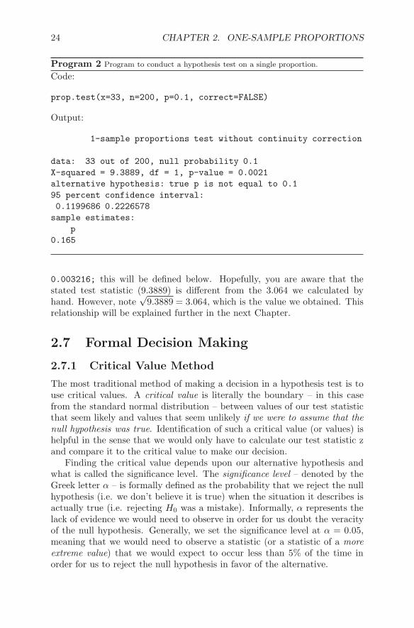
The R code for our example is given in Program 2 below.Notice that R provides a considerable amount of output (some of which

is not needed or has not yet been defined). The data: line states what Ris testing, which corresponds to the x, n and p0. The next line gives thevalue of the test statistic X-squared = 9.3889 and states that p-value =


Program 2 Program to conduct a hypothesis test on a single proportion.

Code:

prop.test(x=33, n=200, p=0.1, correct=FALSE)

Output:

1-sample proportions test without continuity correction

data: 33 out of 200, null probability 0.1

X-squared = 9.3889, df = 1, p-value = 0.0021

alternative hypothesis: true p is not equal to 0.1

95 percent confidence interval:

0.1199686 0.2226578

sample estimates:

p

0.165

0.003216; this will be defined below. Hopefully, you are aware that thestated test statistic (9.3889) is different from the 3.064 we calculated byhand. However, note

√9.3889 = 3.064, which is the value we obtained. This

relationship will be explained further in the next Chapter.

2.7 Formal Decision Making

2.7.1 Critical Value Method

The most traditional method of making a decision in a hypothesis test is touse critical values. A critical value is literally the boundary – in this casefrom the standard normal distribution – between values of our test statisticthat seem likely and values that seem unlikely if we were to assume that thenull hypothesis was true. Identification of such a critical value (or values) ishelpful in the sense that we would only have to calculate our test statistic zand compare it to the critical value to make our decision.

Finding the critical value depends upon our alternative hypothesis andwhat is called the significance level. The significance level – denoted by theGreek letter α – is formally defined as the probability that we reject the nullhypothesis (i.e. we don’t believe it is true) when the situation it describes isactually true (i.e. rejecting H0 was a mistake). Informally, α represents thelack of evidence we would need to observe in order for us doubt the veracityof the null hypothesis. Generally, we set the significance level at α = 0.05,meaning that we would need to observe a statistic (or a statistic of a moreextreme value) that we would expect to occur less than 5% of the time inorder for us to reject the null hypothesis in favor of the alternative.

2.7. FORMAL DECISION MAKING 25

Given a specified significance level (and α = 0.05 is generally used), thecritical value then depends upon our alternative hypothesis. If the alternativespecified that the proportion is less than some specified value (HA : p < p0)then we would expect small sample proportions (or negative values of ourtests statistic z) to be rare if we assume H0 : p = p0 is true, and thus ourcritical value should be negative. For a similar reason, we have a positivecritical value if our alternative hypothesis is HA : p > p0. In cases of a two-sided alternative hypothesis (or HA : p �= p0), we need two critical values,since sample values much greater or much lower than our hypothesized valuewould lead us to reject the null hypothesis. All possible cases and decisionsare presented in Table 2.3 for α = 0.05 and α = 0.01, which are the mostcommonly used significance levels. Thus, rather than having to determinecritical values for each hypothesis test we wish to perform, we can consultTable 2.3 to obtain: (i) the critical value specific to the desired significancelevel and alternative hypothesis, and (ii) the criterion under which we wouldselect the null or alternative hypothesis.

Table 2.3: Critical Values and Rejection (Acceptance) Regions for Hypoth-esis Test of a Proportion for Given Significance Levels (α) and AlternativeHypotheses.

α = 0.05 α = 0.01

Alternative Critical Select Critical SelectHypothesis Value Hypothesis Value Hypothesis

HA : p < p0 −1.645 H0 if z ≥ −1.645 −2.33 H0 if z ≥ −2.33

(Left-Tailed Test)

HA if z < −1.645 HA if z < −2.33

HA : p > p0 1.645 H0 if z ≤ 1.645 2.33 H0 if z ≤ 2.33

(Right-Tailed Test)

HA if z > 1.645 HA if z > 2.33

HA : p �= p0 −1.96, H0 if −2.575, H0 if

(Left-Tailed Test) 1.96 −1.96 ≤ z ≥ 1.96 2.575 −2.575 ≤ z ≥ 2.575

HA if z < −1.96 or HA if z < −2.575 or

z > 1.96 z > 2.575

In our example, say our original research statement was: the proportionof subjects who experience reduced side-effects from this treatment is greaterthan 0.10. This means our null hypothesis isH0 : p = 0.10 and our alternativehypothesis is HA : p > 0.10, and thus our critical value is 1.645 (if we haveα = 0.05), meaning that we will reject H0 in favor of HA if the test statisticis greater than 1.645, and we will not reject H0 if the test statistic is lessthan or equal to 1.645. Earlier, we calculated our test statistic as z = 3.06,


which falls in the rejection region, so we reject H0 in favor of HA. We willdiscuss what this means and how we react later.

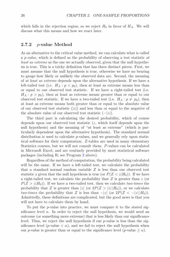
2.7.2 p-value Method

As an alternative to the critical value method, we can calculate what is calleda p-value, which is defined as the probability of observing a test statistic atleast as extreme as the one we actually observed, given that the null hypothe-sis is true. This is a tricky definition that has three distinct pieces. First, wemust assume that the null hypothesis is true, otherwise we have no bearingto gauge how likely or unlikely the observed data are. Second, the meaningof at least as extreme depends upon the alternative hypothesis. If we have aleft-tailed test (i.e. HA : p < p0), then at least as extreme means less thanor equal to our observed test statistic. If we have a right-tailed test (i.e.HA : p > p0), then at least as extreme means greater than or equal to ourobserved test statistic. If we have a two-tailed test (i.e. HA : p �= p0), thenat least as extreme means both greater than or equal to the absolute valueof our observed test statistic (|z|) and less than or equal to the negative ofthe absolute value of our observed test statistic (−|z|).

The third part is calculating the desired probability, which of coursedepends upon our observed test statistic (z, which itself depends upon thenull hypothesis) and the meaning of “at least as extreme” (which is par-ticularly dependent upon the alternative hypothesis). The standard normaldistribution is used to calculate p-values, and we generally rely upon statis-tical software for their computation. Z-tables are used in many elementaryStatistics courses, but we will not consult them. P -values can be calculatedin Microsoft Excel, and are routinely provided by most statistical softwarepackages (including R; see Program 2 above).

Regardless of the method of computation, the probability being calculatedwill be the same. If we have a left-tailed test, we calculate the probabilitythat a standard normal random variable Z is less than our observed teststatistic z given that the null hypothesis is true (or P (Z < z|H0)). If we havea right-tailed test, we calculate the probability that Z is greater than z (orP (Z > z|H0)). If we have a two-tailed test, then we calculate two-times theprobability that Z is greater than |z| (or 2P (Z > |z| |H0)), or we calculatetwo-times the probability that Z is less than −|z| (or 2P (Z < −|z| |H0)).Admittedly, these definitions are complicated, but the good news is that youwill not have to calculate them by hand.

To put the p-value into practice, we must compare it to the stated sig-nificance level α. In order to reject the null hypothesis, we would need anoutcome (or something more extreme) that is less likely than our significancelevel. Thus, we reject the null hypothesis if our p-value is less than the sig-nificance level (p-value < α), and we fail to reject the null hypothesis whenour p-value is greater than or equal to the significance level (p-value ≥ α).

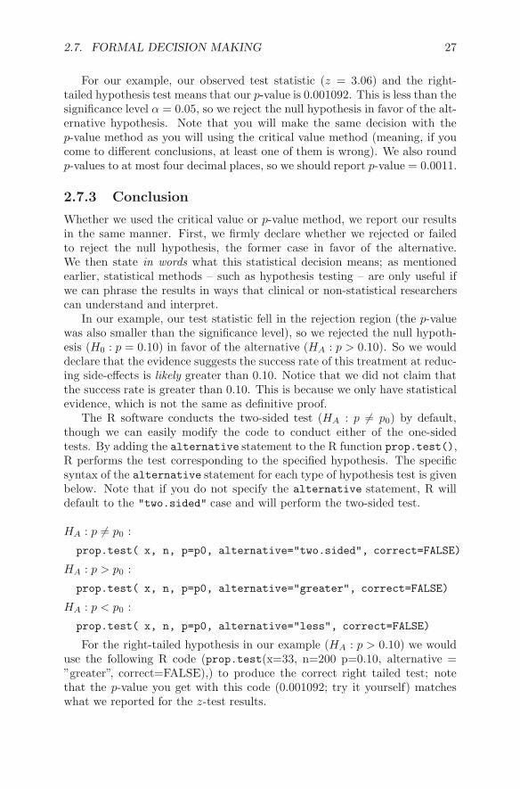
2.7. FORMAL DECISION MAKING 27

For our example, our observed test statistic (z = 3.06) and the right-tailed hypothesis test means that our p-value is 0.001092. This is less than thesignificance level α = 0.05, so we reject the null hypothesis in favor of the alt-ernative hypothesis. Note that you will make the same decision with thep-value method as you will using the critical value method (meaning, if youcome to different conclusions, at least one of them is wrong). We also roundp-values to at most four decimal places, so we should report p-value = 0.0011.

2.7.3 Conclusion

Whether we used the critical value or p-value method, we report our resultsin the same manner. First, we firmly declare whether we rejected or failedto reject the null hypothesis, the former case in favor of the alternative.We then state in words what this statistical decision means; as mentionedearlier, statistical methods – such as hypothesis testing – are only useful ifwe can phrase the results in ways that clinical or non-statistical researcherscan understand and interpret.

In our example, our test statistic fell in the rejection region (the p-valuewas also smaller than the significance level), so we rejected the null hypoth-esis (H0 : p = 0.10) in favor of the alternative (HA : p > 0.10). So we woulddeclare that the evidence suggests the success rate of this treatment at reduc-ing side-effects is likely greater than 0.10. Notice that we did not claim thatthe success rate is greater than 0.10. This is because we only have statisticalevidence, which is not the same as definitive proof.

The R software conducts the two-sided test (HA : p �= p0) by default,though we can easily modify the code to conduct either of the one-sidedtests. By adding the alternative statement to the R function prop.test(),R performs the test corresponding to the specified hypothesis. The specificsyntax of the alternative statement for each type of hypothesis test is givenbelow. Note that if you do not specify the alternative statement, R willdefault to the "two.sided" case and will perform the two-sided test.

HA : p �= p0 :

prop.test( x, n, p=p0, alternative="two.sided", correct=FALSE)

HA : p > p0 :

prop.test( x, n, p=p0, alternative="greater", correct=FALSE)

HA : p < p0 :

prop.test( x, n, p=p0, alternative="less", correct=FALSE)

For the right-tailed hypothesis in our example (HA : p > 0.10) we woulduse the following R code (prop.test(x=33, n=200 p=0.10, alternative =”greater”, correct=FALSE),) to produce the correct right tailed test; notethat the p-value you get with this code (0.001092; try it yourself) matcheswhat we reported for the z-test results.


2.7.4 Confidence Intervals

The sample proportion p̂ is dependent upon the sample we collect and theparticular subjects observed within that sample. In other words, p̂ maychange if we collect a different sample consisting of different subjects. Thisis a source of variability that is not expressed if we focus solely upon thecurrent sample estimate. Thus, we often accompany each sample estimatewith a confidence interval that takes into account sampling variability.

A confidence interval is straight forward to calculate, though somewhattricky to define. What is definitive is what a confidence interval is not. A con-fidence interval has a stated level of confidence (defined as the complementof the stated significance level, or 1 − α). For instance, if our significancelevel is 0.05, then our confidence level is 1− 0.05 = 0.95, and we would thenconstruct a 95% confidence interval. This level of confidence is often takenas the quantification of our belief that the true population parameter resideswithin the estimated confidence interval; this is false. Once calculated, a pop-ulation parameter is either in a confidence interval or it is not. Rather, theconfidence level reflects our belief in the process of constructing confidenceintervals, so that we believe that 95% of our estimated confidence intervalswould contain the true population parameter, if we could repeatedly samplefrom the same population. This is an important distinction that underlieswhat classical statistical methods and inference can and cannot state (i.e.we don’t know anything about the population parameter, only our sampledata).

To calculate a (1− α)% confidence interval (or CI) we need three things:a point estimate, a measure of variability of that point estimate, and a prob-abilistic measure that distinguishes between likely and unlikely values of ourpoint estimate. With these three pieces, our CI would take the form:

(Point Estimate ± Measure of Variability × Probabilistic Measure)

The ± sign indicates that by adding and subtracting the second part fromthe first we will obtain the upper and lower bounds, respectively, of ourconfidence interval. For a point estimate we use p̂; in our example, thisvalues is 0.165. As a measure of variability, we will use the square root ofp̂(1− p̂)/n, which is similar to the standard error used in hypothesis testing,except here we use p̂ instead of p0 since we don’t necessarily want to use anull hypothesis to summarize our data (e.g. sometimes we may only want theCI and not the hypothesis test). Based on our sample data, this value wouldbe SE =

√0.165(1− 0.165)/200 = 0.026. As a probabilistic measure, we

use the positive critical value from a two-tailed test for the given confidencelevel. For instance, if we want 95% confidence, then we would have α = 0.05,and a two-tailed test would yield critical values ±1.96, of which we take thepositive value 1.96. Putting these values from our example together, our 95%confidence interval is

(0.165− 1.96× 0.026, 0.165+ 1.96× 0.026) = (0.114, 0.216)

2.8. CONTINGENCY METHODS (WITH R CODE) 29

To interpret this interval, we would say “a 95% confidence interval of thepopulation proportion of subjects who experienced reduced side-effects withthis treatment is (0.114, 0.216)”. In general, we round the confidence intervalto the same degree of precision as our point estimate, in this case the sampleproportion. Note that some researchers use confidence intervals to conducthypothesis tests, where they estimate a confidence interval and determinewhether some hypothesized value is within the interval (if not, reject H0;if so, fail to reject H0). While the confidence interval approach is similar inmany ways to hypothesis testing, they are not the same and may not producethe same inference. For this and other reasons, we will use confidence intervalsonly as a form of data summarization, and will not use them for inference. Forthe record, we do not recommend or condone the use of confidence intervalsfor making statistical decisions or inference, and strongly encourage you torefrain from this practice.

Note that we could have used R to produce this confidence interval, butit will not immediately be the same, since R calculates confidence intervalsusing what is called the “continuity correction”. This adjustment and theresulting type of interval is an equally valid but all together different typeof confidence interval than the method described above; note that what welearned is by far the most commonly accepted form of calculating confidenceintervals for dichotomous data. Moving forward, you can choose to calculate95% CIs on a proportion using the method outlined in this chapter (whichrequires you to calculate the interval by hand), or you may use the twomethods provided by the R software. To get the 95% CI in R, we make useof the prop.test() function with the following specifications (x=33, n=200,p=0.1, alternative=”two.sided”), which produces a 95% CI of (0.118, 0.225).Note that this method uses what’s called the continuity correction, whichwe can turn off by specifying “correct=False” in the prop.test() function,which gives a 95% CI of (0.120, 0.223). Both of these intervals are similarto but not equal to the interval provided above (0.114, 0.216); ultimately, wewould have to create our own code in R (which is not too difficult) to obtainthe confidence interval we obtained by hand.

2.8 Contingency Methods (with R Code)

Occasionally we will experience the situation where we wish to compare theproportion to some hypothesized value, but (at least) one of our expectedfrequencies is less than 5, meaning we do not have a large enough sample sizeto perform the z-test. In that case, we must instead use the Binomial Test,which is a test that compares the proportion to a hypothesized standard andis valid for any sample size. This test works for any sample size because itis based on the concept of enumeration, or counting all possible outcomesthat could be observed within one group of categorical data. In this instanceenumerating all possible outcomes is not difficult, and can even be done byhand when the sample sizes are small enough.


For instance, imagine the case where someone gives you a cup and tellsyou it is either filled with Pepsi or Coke (let’s say it is actually Pepsi). If youwere asked to taste the soda and guess which soda was in which cup, there areonly two possible outcomes: you guess correctly or incorrectly. This scenariois numerically represented in Table 2.4. If we had no way to discern betweenthe unique tastes of Pepsi and Coke (i.e we were simply guessing), then wewould assume that either outcome (we guess correctly or incorrectly) wouldhave the same probability (0.5). Given this assumption (which is our nullhypothesis), we can calculate the p-value of having as many or more correctguesses than what we observed. Based on the one-cup experiment (Table 2.4),if we were to guess 0 correct, then the p-value = 1.0, because we are certainof getting an outcome at least as extreme as the one we got (i.e. 0 or morecorrect) the next time we do this experiment. If we guessed correctly, thenthe p-value = 0.5, meaning there is an equal likelihood of getting a 1 or 0 thenext time we do this experiment (the “1” being at least as extreme). Bothp-values are much larger than 0.05, so even if we selected correctly, this isnot enough evidence for us to reject the null hypothesis.

Table 2.4: Enumeration of Outcomes from One-Cup Experiment (Y: CorrectGuess, N: Incorrect Guess).

Actual Soda in CupPepsi # Correct Frequency Proportion p-valueN 0 1 0.5 0.5+0.5 = 1.0Y 1 1 0.5 0.5

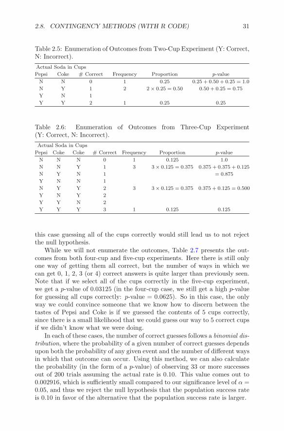
Now let’s assume that we have two cups, where the first is filled withPepsi and the other with Coke. Of course, we do not know which sodas areactually in each cup, so we could guess that they are both filled with Pepsi,they are both filled with Coke, or they are filled with one soda each (andthere are two ways in which this can happen: Pepsi in the first and Cokein the second, or Coke in the first and Pepsi in the second). Thus there arefour ways in which we can guess, one resulting in no correct guesses, tworesulting in one correct guess (and one incorrect guess), and one resultingin two correct guesses. These outcomes are summarized in Table 2.5. Sincethe four outcomes are equally probable if we are only guessing (assuming thenull hypothesis is true), then each particular outcome has a 0.25 chance ofoccurring. So in this case, even if we guess the contents of both cups correctly,our p-value (0.25) would still not lead us to reject the null hypothesis.

If we have three cups (filled with Pepsi, Coke and Coke, respectively),there are now eight possible ways in which we can guess, which lead to 0, 1,2 or 3 correct guesses. The possibilities are listed in Table 2.6. Here we seethat even if we were to guess correctly the contents of each cup, the evidencethat we actually know what we are doing is still low (p-value = 0.125). So in

2.8. CONTINGENCY METHODS (WITH R CODE) 31

Table 2.5: Enumeration of Outcomes from Two-Cup Experiment (Y: Correct,N: Incorrect).

Actual Soda in Cups

Pepsi Coke # Correct Frequency Proportion p-value

N N 0 1 0.25 0.25 + 0.50 + 0.25 = 1.0

N Y 1 2 2× 0.25 = 0.50 0.50 + 0.25 = 0.75

Y N 1

Y Y 2 1 0.25 0.25

Table 2.6: Enumeration of Outcomes from Three-Cup Experiment(Y: Correct, N: Incorrect).

Actual Soda in Cups

Pepsi Coke Coke # Correct Frequency Proportion p-value

N N N 0 1 0.125 1.0

N N Y 1 3 3× 0.125 = 0.375 0.375 + 0.375 + 0.125

N Y N 1 = 0.875

Y N N 1

N Y Y 2 3 3× 0.125 = 0.375 0.375 + 0.125 = 0.500

Y N Y 2

Y Y N 2

Y Y Y 3 1 0.125 0.125

this case guessing all of the cups correctly would still lead us to not rejectthe null hypothesis.

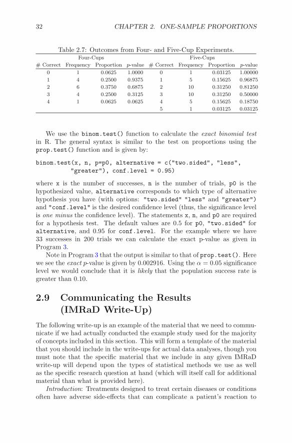
While we will not enumerate the outcomes, Table 2.7 presents the out-comes from both four-cup and five-cup experiments. Here there is still onlyone way of getting them all correct, but the number of ways in which wecan get 0, 1, 2, 3 (or 4) correct answers is quite larger than previously seen.Note that if we select all of the cups correctly in the five-cup experiment,we get a p-value of 0.03125 (in the four-cup case, we still get a high p-valuefor guessing all cups correctly: p-value = 0.0625). So in this case, the onlyway we could convince someone that we know how to discern between thetastes of Pepsi and Coke is if we guessed the contents of 5 cups correctly,since there is a small likelihood that we could guess our way to 5 correct cupsif we didn’t know what we were doing.

In each of these cases, the number of correct guesses follows a binomial dis-tribution, where the probability of a given number of correct guesses dependsupon both the probability of any given event and the number of different waysin which that outcome can occur. Using this method, we can also calculatethe probability (in the form of a p-value) of observing 33 or more successesout of 200 trials assuming the actual rate is 0.10. This value comes out to0.002916, which is sufficiently small compared to our significance level of α =0.05, and thus we reject the null hypothesis that the population success rateis 0.10 in favor of the alternative that the population success rate is larger.


Table 2.7: Outcomes from Four- and Five-Cup Experiments.Four-Cups Five-Cups

# Correct Frequency Proportion p-value # Correct Frequency Proportion p-value

0 1 0.0625 1.0000 0 1 0.03125 1.00000

1 4 0.2500 0.9375 1 5 0.15625 0.96875

2 6 0.3750 0.6875 2 10 0.31250 0.81250

3 4 0.2500 0.3125 3 10 0.31250 0.50000

4 1 0.0625 0.0625 4 5 0.15625 0.18750

5 1 0.03125 0.03125

We use the binom.test() function to calculate the exact binomial testin R. The general syntax is similar to the test on proportions using theprop.test() function and is given by:

binom.test(x, n, p=p0, alternative = c("two.sided", "less",

"greater"), conf.level = 0.95)

where x is the number of successes, n is the number of trials, p0 is thehypothesized value, alternative corresponds to which type of alternativehypothesis you have (with options: "two.sided" "less" and "greater")

and "conf.level" is the desired confidence level (thus, the significance levelis one minus the confidence level). The statements x, n, and p0 are requiredfor a hypothesis test. The default values are 0.5 for p0, "two.sided" foralternative, and 0.95 for conf.level. For the example where we have33 successes in 200 trials we can calculate the exact p-value as given inProgram 3.

Note in Program 3 that the output is similar to that of prop.test(). Herewe see the exact p-value is given by 0.002916. Using the α = 0.05 significancelevel we would conclude that it is likely that the population success rate isgreater than 0.10.

2.9 Communicating the Results

(IMRaD Write-Up)

The following write-up is an example of the material that we need to commu-nicate if we had actually conducted the example study used for the majorityof concepts included in this section. This will form a template of the materialthat you should include in the write-ups for actual data analyses, though youmust note that the specific material that we include in any given IMRaDwrite-up will depend upon the types of statistical methods we use as wellas the specific research question at hand (which will itself call for additionalmaterial than what is provided here).

Introduction: Treatments designed to treat certain diseases or conditionsoften have adverse side-effects that can complicate a patient’s reaction to

2.9. COMMUNICATING THE RESULTS (IMRAD WRITE-UP) 33

Program 3 Program to conduct an exact hypothesis test on a single proportion.

Code:

binom.test(x=33, n=200, p=0.1, alternative="greater")

Output:

Exact binomial test

data: 33 and 200

number of successes = 33, number of trials = 200, p-value =

0.002916

alternative hypothesis: true probability of success is

greater than 0.1

95 percent confidence interval:

0.1232791 1.0000000

sample estimates:

probability of success

0.165

the treatment, and can ultimately result in a worse disease or conditionprognosis. Clinicians and practitioners are then interested in treatments thathave minimal to no side-effects. It was of interest to determine whether theproportion of patients undergoing a particular treatment who experiencedlittle to no adverse side-effects was greater than 0.10.

Methods: The frequency of subjects reporting reduced side-effects fromtreatment out of 200 subjects is reported, and the proportion of subjectsreporting reduced side-effects is summarized with a sample proportion anda 95% confidence interval. We test the null hypothesis of a 0.10 success rate(H0 : p = 0.10) against a one-sided alternative hypothesis that the successrate is greater than 0.10 (HA : p > 0.10) by using a chi-square-test withsignificance level α = 0.05. We will reject the null hypothesis in favor of thealternative hypothesis if the p-value is less than α; otherwise we will not re-ject the null hypothesis. The R statistical software was used for all analyses.

Results: Assuming that the sample was representative and subjects wereindependent, the sample was large enough to conduct the statistical analy-sis. Out of a sample of 200 total patients, 33 reported reduced symptoms(p̂ = 0.165, 95%CI : 0.120, 0.223). Using this data, a chi-square test yieldeda p-value of 0.0011, which is less than the stated significance level. Thus, wereject the null hypothesis in favor of the alternative hypothesis.

Discussion: The sample data suggest that the proportion of patientswho reported reduced side-effects using this treatment is greater than 0.10.Thus, clinicians and practitioners interested in treating patients with reducedtreatment-related side-effects may wish to consider this treatment.


2.10 Process

1. State research question in form of testable hypothesis.

2. Determine whether assumptions are met.

(a) Representative sample.

(b) Independent measurements.

(c) Sample size: calculate expected frequencies

i. If np0 > 5 and n(1 − p0) > 5, then use z-test or chi-squaretest (in R).

ii. If np0 < 5 or n(1− p0) < 5, then use binomial test.

3. Summarize data.

(a) If np0 > 5 and n(1− p0) > 5, then report: frequency, sample size,sample proportion and CI.

(b) If np0 < 5 or n(1 − p0) < 5, then report: frequency and samplesize.

4. Calculate test statistic.

5. Compare test statistic to critical value or calculate p-value.

6. Make decision (reject H0 or fail to reject H0).

7. Summarize with IMRaD write-up.

2.11 Exercises

1. A researcher is interested in the proportion of active duty police offi-cers who pass the standard end of training fitness test. They take arandom sample of 607 officers from a major metropolitan police forceand administer the fitness test to the officers. They find that 476 ofthe officers were able to successfully pass the fitness test. Create 96%confidence interval for the proportion of all active duty police officerson the police force that can pass the fitness test.

2. Occupational health researchers are interested in the health effects ofsedentary occupations such as call center workers. Specifically they areinterested in lower back pain. They conduct a survey of 439 call centerworkers and record whether or not the worker has back pain at theend of their shift. The surveys show that 219 workers reported backpain. In the general population there are reports that 25% of workershave back pain. Conduct a hypothesis test to determine if call centerworkers have a higher rate of back pain than the general population ofworkers.

2.11. EXERCISES 35

3. In December 2012 Gallup Poll conducted a survey of 1,015 Americansto determine if they had delayed seeking healthcare treatment due tothe associate costs. Of the participants, 325 reported delaying seekingtreatment due to costs. Create a 95% confidence interval for the pro-portion of all Americans who have delayed seeking healthcare treatmentdue to costs.

4. Norman et al. (2013) Consider the preference for walkability of neigh-borhoods for obese men. They studied 240 obese men and asked themtheir preference for walking behavior in neighborhoods. They foundthat 63 responded as they walked for transportation. Create a 99%confidence interval for the proportion of obese men who walk for trans-portation.

5. Barrison et al. (2001) are interested in the reasons that proton pumpinhibitors were prescribed. Of the 182 gastroenterologists 122 of themprescribed proton pump inhibitors to patients. Create a 98% confidenceinterval for the proportion of all gastroenterologists who prescribe pro-ton pump inhibitors.

6. Barrison et al. (2001) were interested in the proportion of physicianswho deemed that proton pump inhibitors (PPI) should be sold overthe counter. Of the 391 physicians surveyed 59 responded that PPIsshould be sold over the counter. Create a 92% confidence interval forthe proportion of physicians who think that PPIs should be sold overthe counter.

7. Keightley et al. (2011) are concerned with obese peoples self percep-tions. They hypothesize that a majority of obese people can identifytheir own body type. They conduct a study with 87 obese people andfind that 7 can correctly identify their body type. Conduct a hypothesistest to determine whether or not their hypothesis is warranted.

8. Salerno et al. (2013) is interested in determining the current infectionrate of Chlamydia and Gonorrhea infections. They obtained a sampleof 508 high school students who consented to a urine test to screen forthe two diseases. Of the participants 46 tested positive for at least oneof the diseases. Create a 99% confidence interval for the proportion ofall high school students who have one of the two diseases.

http://www.springer.com/978-1-4614-8707-4

One-Sample Proportions

Documents

Transcript of One-Sample Proportions