One for all? The capital-labour substitution elasticity in ... · The capital-labour substitution...
40
One for all? The capital-labour substitution elasticity in New Zealand, by Adam Tipper One for all? The capital-labour substitution elasticity in New Zealand Paper prepared for the 52 nd New Zealand Association of Economists conference, Wellington, New Zealand, June 2011 Adam Tipper Macroeconomic Statistics Development Unit, Statistics New Zealand P O Box 2922 Wellington, New Zealand [email protected] +64 (0)4 931 4944 www.stats.govt.nz Liability The opinions, findings, recommendations, and conclusions expressed in this paper are those of the author. They do not represent those of Statistics New Zealand, which takes no responsibility for any omissions or errors in the information in this paper. Citation Tipper, A (2011, June). One for all? The capital-labour substitution elasticity in New Zealand. Paper prepared for the 52 nd New Zealand Association of Economists conference, Wellington, New Zealand.
Transcript of One for all? The capital-labour substitution elasticity in ... · The capital-labour substitution...

One for all? The capital-labour substitution elasticity in New Zealand, by Adam Tipper
One for all? The capital-labour substitution elasticity in New Zealand
Paper prepared for the 52nd New Zealand Association of Economists conference, Wellington, New Zealand,
June 2011
Adam Tipper
Macroeconomic Statistics Development Unit, Statistics New Zealand
P O Box 2922 Wellington, New Zealand
[email protected] +64 (0)4 931 4944
www.stats.govt.nz
Liability The opinions, findings, recommendations, and conclusions expressed in this paper are those of the author. They do not represent those of Statistics New Zealand, which takes no responsibility for any omissions or errors in the information in this paper. Citation Tipper, A (2011, June). One for all? The capital-labour substitution elasticity in New Zealand. Paper prepared for the 52
nd New Zealand Association of Economists conference, Wellington, New Zealand.
One for all? The capital-labour substitution elasticity in New Zealand, by Adam Tipper
2
Abstract
This paper tests the assumption of a Cobb-Douglas production function (a unitary elasticity
of substitution between capital and labour) for 20 of New Zealand’s industries using
Statistics New Zealand’s industry-level productivity data. It also assesses how the Leontief
production function (zero substitutability) may apply to New Zealand industries. The
econometric estimates of the capital-labour substitution elasticity provide some evidence for
the Cobb-Douglas assumption at sector and industry level in the long-run, but show the
Leontief function is more appropriate in the short-run. These results facilitate interpretation of
the industry-level productivity data, highlight the variation in substitutability across industries
and sectors, and suggest existing official multifactor productivity estimates may be biased
downwards.
Keywords: Capital-labour substitution; multifactor productivity; Cobb-Douglas; Leontief
JEL codes: D24; E23; O47
Introduction
Determining New Zealand’s productive capability relies on an understanding of the role of
inputs in producing outputs. Value-added growth can come from growth in labour inputs,
capital inputs, or multifactor productivity (MFP). However, calculating MFP (as a residual)
depends on the specification of the relationship between labour and capital in the production
function (which shows how inputs are used to create output). Increases in wages, while
assuming the returns to capital are constant, should result in an appropriate adjustment of
labour relative to capital. But to what extent does that substitution take place and, if the
substitution is not as strong as expected, how might our understanding of the contributors to
output growth change? The relationship between capital and labour is also likely to differ
across industries due to the nature of demand for a given industries output. An examination
of the assumption of one production function (and an elasticity equal to one) for all industries
is thus pertinent in understanding industry drivers of macroeconomic growth.
There are a range of possible forms of the production function, each of which has
implications for the measurement of MFP. The calculation of Statistics NZ’s MFP series
assumes that the production function is of the Cobb-Douglas form (where each factor of
production is exponentially weighted by its income share, there are constant returns to scale,
and markets are perfectly competitive). The Cobb-Douglas framework assumes that there is
a unitary elasticity of substitution between capital and labour inputs (henceforth the
elasticity). This means a unit increase in the ratio of wages to rental-prices is matched by a
unit increase in the capital-to-labour ratio. The elasticity measures how easy it is for an
economy, sector, or industry, to adjust its inputs as the price of labour changes relative to
the price of capital. An alternative to the Cobb-Douglas function is the Leontief function,
where it is assumed that labour and capital cannot be substituted. Both of these functions
are specific cases of the general constant elasticity of substitution function, which allows the

One for all? The capital-labour substitution elasticity in New Zealand, by Adam Tipper
3
elasticity to be between zero and one, or even greater than one. As MFP (viewed as a
measure of technological change when the production function is Cobb-Douglas and output
is measured by value added) is dependent on the specification of the inputs to production,
assessing the validity of this assumption is key to verifying the estimates for MFP (ie mis-
specification of the production function can bias MFP estimates). While this assumption is
applied uniformly to each industry, and to the measured sector aggregate, the diverse nature
of industries indicates that this form of the production function may not be applicable to all
industries. For example, a hairdresser is always required to perform a haircut, but the labour
of a factory worker can become automated.
The value of the elasticity is also an important parameter in general equilibrium models.
However, some models currently use estimates based on Australian data, which may not
reflect New Zealand’s market activity. Zuccollo (2011), for example, demonstrates the impact
of using New Zealand specific elasticities on economic growth following a reduction in tariffs.
The degree of input substitution may also be useful in assessing the likely efficacy of policy
that aims to use the price mechanism to increase capital per worker and (ultimately) labour
productivity. In addition, the elasticity can be used to explain whether capital accumulation is
a driver of growth in real unit labour costs (Lebrun and Perez, 2011).
A lack of appropriate data has previously hampered attempts to estimate the elasticity and
therefore the form of the production function in New Zealand. However, Statistics NZ’s
industry-level productivity data, first released in June 2010, provide the required income and
volume data, for both capital and labour inputs, that are necessary to test the Cobb-Douglas
assumption. These data can be used to assess the relationship between the capital-to-
labour ratio and the wage-rental price ratio, and allow econometric tests of the assumption of
a unitary elasticity. This framework can also be used to test the assumption underlying the
Leontief function, that capital and labour are assumed to exhibit zero substitutability.
This paper tests the assumption that a Cobb-Douglas production function is applicable to all
industries. The data used in this paper are taken from Statistics NZ’s industry-level
productivity statistics series, which covers 24 industries from 1978 to 2009. To provide
reasonable estimates at the industry level, data are for the Australian New Zealand Standard
Industrial Classification 1996 (ANZSIC96) industries A to K (see appendix B for a definition
of these industries). Property services, business services, cultural and recreational services,
and personal and other community services are excluded from the industry-level analysis as
their series begin in 1996, and thus provide too few observations for time series models.
Estimates of the elasticity for the former measured sector, three core sectors, and 20 of New
Zealand’s industries are presented in this paper. The econometric methodology follows that
of Balistreri, McDaniel, and Wong (2003) who assessed the assumption of a Cobb-Douglas
production function using United States’ (US) industry-level data. This approach allows for
both short and long-run elasticities to be derived, and for an assessment of the dynamic
nature of capital accumulation decisions. However, the theoretical motivation differs. It
emphasises the importance of specifying the form of the production function for interpreting
and calculating MFP. It begins with an overview of capital-labour substitution and an
explanation of how the degree of substitution varies depending on assumptions regarding
the production function. Econometric techniques are then used to estimate the elasticity. The
discussion outlines what these findings may mean for the estimation of measured sector,
sector, and industry-level MFP. While there is some evidence to support the Cobb-Douglas
One for all? The capital-labour substitution elasticity in New Zealand, by Adam Tipper
4
approach to estimating productivity, it is not appropriate for all industries. In the short-run
especially, the Leontief function fits the data better. These estimates may be useful in
interpreting and understanding the robustness of the industry-level MFP data, and for
undertaking sensitivity analysis in broader general equilibrium models.
Capital-labour substitution
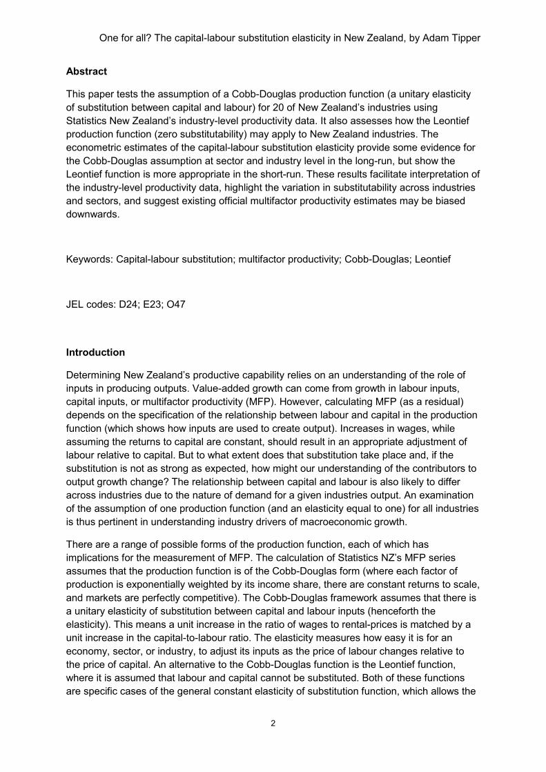
The concept of capital-labour substitution is illustrated in figure 1. A neoclassical framework
is used to show the (concave) production possibility frontier (north-west quadrant) of an
industry using capital K and labour L. Under perfect competition, industries always operate
on the frontier. At any point on this curve, the same amount of output V can be produced
from any combination of labour and capital input. The slope of the frontier reflects the
marginal rate of technical substitution (the ratio of relative factor prices). Assuming
diminishing marginal returns from each factor of production, the production functions for
capital and labour can be plotted (north-east and south-west quadrants).
Figure 1: The production possibility frontier, production functions, and capital-labour
isoquant in a Cobb-Douglas economy
Suppose that the industry decides to reduce its capital input but maintain the same level of
output. This leads to a movement along the production possibility frontier and along the
production function for labour. The amount of labour used in production can then be
K
L
Vk=f(K)
VK
VL
Production possibility
frontier
VL=f(L)
Capital-labour
isoquant
One for all? The capital-labour substitution elasticity in New Zealand, by Adam Tipper
5
compared against the amount of capital (south-east quadrant). Repeating this exercise
reveals a convex relationship between capital and labour inputs (known as the isoquant).
This is the standard Cobb-Douglas result and is dependent on the assumption of diminishing
marginal returns.
As the slope of the production possibility frontier is equal to the ratio of relative factor prices
and the capital-to-labour ratio is derived from the points on the frontier, relative movements
along the frontier (ie reflecting a changing slope in the budget constraint), and
correspondingly the isoquant, affect the elasticity. Under the Cobb-Douglas framework, the
value of the elasticity is equal to unity. It is important to note that shifts in the frontier reflect
pure disembodied technological change (ie are independent of increased use of existing
resources or price changes).
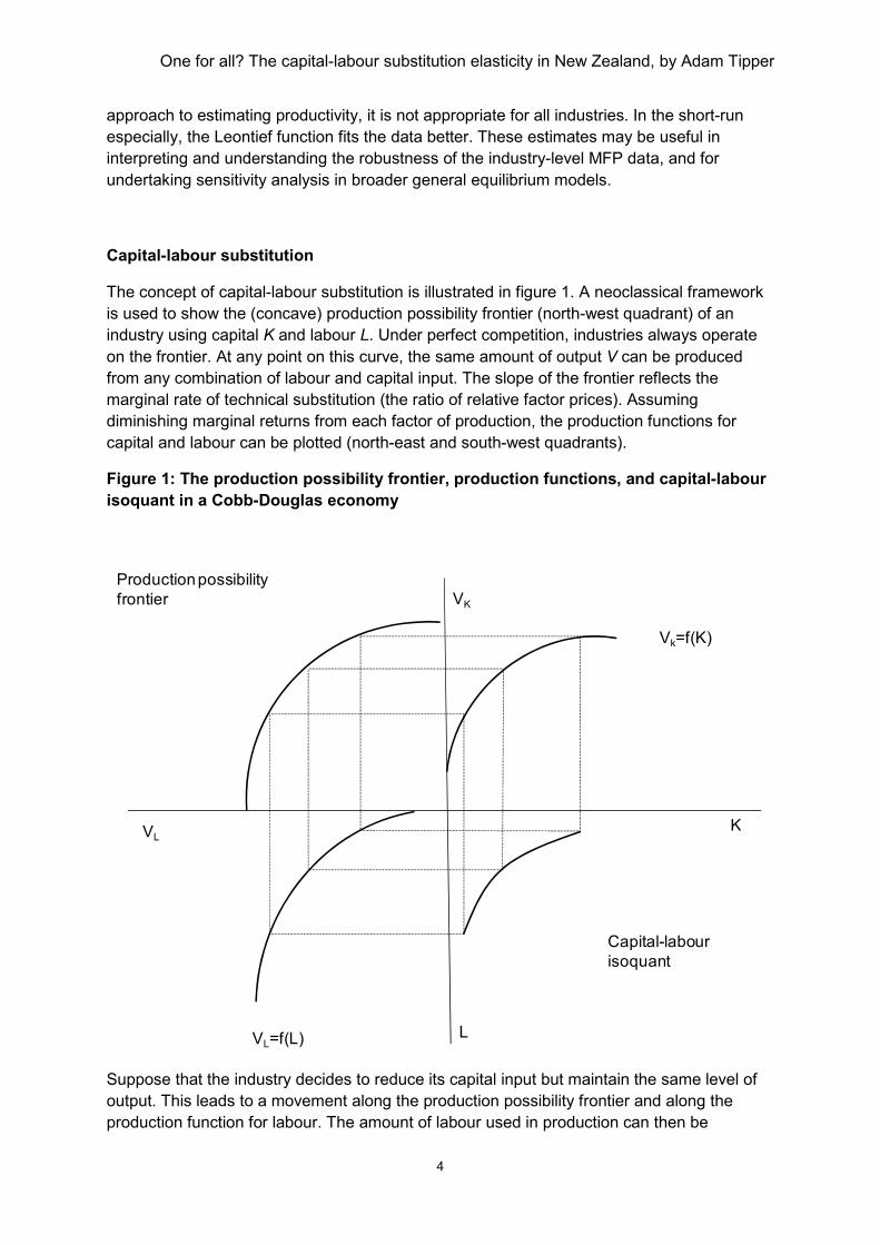
Figure 2: The production possibility frontier, production functions, and capital-labour isoquant in a Leontief economy
Sketching a similar pattern for zero substitution is problematic. The shape of the production
possibility frontier is not concave in the short-run (Takamasu, 1986). However, it is likely to
be concave in the long-run, as the short-run frontier is subsumed by the long-run frontier
(Landon, 1990). Typically, the frontier and production functions exhibit kinks (see figure 2).
Again, moving along the frontier (to reflect changing relative prices) leads to an L-shaped
K
L
Vk=f(K)
VK
VL
Production possibility
frontier
VL=f(L)
Capital-labour
isoquant

One for all? The capital-labour substitution elasticity in New Zealand, by Adam Tipper
6
isoquant and shows that the capital-to-labour ratio is independent from such changes. The
equilibrium amount of capital and labour used in production is at the corner of the isoquant.
There are strong arguments for using the Cobb-Douglas approach. Economically, this
approach satisfies the requirements of Kaldor’s stylised facts, which are required for the
construction of economic growth models (Balistreri et al., 2003). The Cobb-Douglas
approach is widely used, so results can easily be compared across statistical agencies. The
core statistical advantage of the assumption is that labour and capital inputs can be
weighted by their current price value-added shares. The Cobb-Douglas assumption has
been tested rigorously, with a number of studies suggesting that it does provide reasonable
estimates of the relationship between capital and labour inputs in the production process.
Balistreri et al. (2003) found that the Cobb-Douglas function could not be rejected in 20 out
of 28 US industries, and also rejected the Leontief function in seven of those industries.
Pendharkar, Rodger, and Subramanian (2008) also find evidence for Cobb-Douglas in a
study of software development firms. Fraser (2002) finds some evidence for the Cobb-
Douglas function in aggregate New Zealand data from 1920-1940.
The Cobb-Douglas approach has, however, often been criticised for its inflexibility. This
debate was sparked by Arrow, Chenery, Minhas, and Solow’s seminal work (1961), which
proposed a contending function to the two predecessors, namely the Cobb-Douglas and
Leontief functions. Motivated by strong empirical evidence that the substitution between
capital and labour is often not equal to unity in US manufacturing firms, Arrow et al.
proposed the constant elasticity of substitution (CES) function where capital and labour can
be substituted at a constant rate but at a value other than unity.
Controversies over the form of aggregate and industry-level production functions remain
today. Bhanumurthy (2002) defends the Cobb-Douglas approach by arguing that many of
the econometric problems posed in estimation can readily be addressed. In outlining the
history of controversies surrounding the form of the aggregate production function, Felipe
and McCombie (2005) argue that the lack of microeconomic foundations challenges the
assumption that the aggregate production function is of the Cobb-Douglas form. Houthakker
(1955), for example, showed that an aggregate Cobb-Douglas function could be derived
from linear activities. Although often used to represent behaviour for economic aggregates,
the Cobb-Douglas function was designed to assess activity at the firm (or microeconomic
level). Its use in macroeconomics has not considered the microeconomic foundations on
which it can be based. Thus, a Cobb-Douglas function for the macro-economy does not
necessarily apply to all industries or vice versa. In addition, statistical evidence in support of
an aggregate Cobb-Douglas function does not necessarily reveal the true underlying
technology of the micro-level components (Felipe and McCombie, 2005).
Recent international empirical evidence refutes the Cobb-Douglas assumption. Chirinko,
Fazzari, and Meyer (2004) estimate the elasticity to be 0.4 rather than unity. Barnes, Price
and Barriel (2008) also find evidence that the elasticity is approximately 0.4 using firm-level
data from the United Kingdom. Lebrun and Perez (2011) suggest that the elasticity is
approximately 0.7. Upender (2009) finds strong supporting evidence for the CES formulation
in a study of Indian industries while Raval (2011) finds no supporting evidence for the Cobb-
Douglas function in US manufacturing firms. However, true elasticities may be much greater
than those often observed due to outliers or ‘shocks’. Regression specification error, such as
including too few lagged variables, may also bias elasticity estimates.
One for all? The capital-labour substitution elasticity in New Zealand, by Adam Tipper
7
Although the elasticity may not be equal to one, it is also debatable whether it is constant
over time. Balk (2010) notes that “the environment in which production units operate is not
so stable as the assumption of a fixed production seems to claim” (p. S225). The fixed
nature of inputs in the short-term, labour and capital market frictions (eg barriers to moving
freely between jobs and time required to learn how to use capital), growth in labour- or
capital-augmenting technology, and sticky wages and prices contribute to this instability. In
the long-term, however, many of these issues should not pervade. One factor which is likely
to have a persisting impact is the changing nature of capital inputs used in the production
process. The advent of information technology in particular may have affected the degree of
substitution between capital and labour over time (Jalava, Pohjola, Ripatti, and Vilmunen,
2006), which suggests different relationships between capital and labour over the first and
last parts of the series. The notion of a non-constant elasticity is supported empirically by
Konishi and Nishiyama’s (2002) study of Japanese manufacturing firms. The study showed
that the elasticity in this industry has changed over time. A time varying elasticity may lead to
some industries showing Cobb-Douglas technology in one period and Leontief in another.
At the industry level, the choice of function may be important as industries differ in the way
they mix their labour and capital inputs. For example, how might a highly capital-intensive
industry adjust its capital and labour if wages increase sharply relative to payments to
capital? A similar question can be posed for labour-intensive industries. If wages increase
relative to payments to capital, but capital cannot be substituted for labour and a certain
amount of labour is required, the elasticity should be minimal. The relevance of the
assumption of uniform production functions for industry-level analysis was summarised by
Carlaw and Lipsey (cited in Mawson, Carlaw, and McLellan, 2003) who stated that:
Given what we know about technological complementarities and the need to adapt
technologies for specific uses, identical production functions across industries is not an
acceptable assumption. For example, it is difficult to believe that the application of electricity
to communications technologies can be considered to be the same production technology as
the application of electricity to mining or machining? (p.15)
In other words, Cobb-Douglas might be an appropriate assumption for one industry, but the
Leontief function (or another function) might be applicable in another. Holding the relative
prices of labour and capital constant, there may be relatively low substitutability in agriculture
and transport and storage, as labour and capital inputs have tracked similarly over the last
three decades (Statistics New Zealand, 2011a). This leads to the labour productivity, capital
productivity, and MFP estimates tracking similarly. The substitutability, however, depends on
the ratio of wages relative to rental-prices. As discussed later, this ratio can be derived as
the ratio of labour income divided by the labour input index to capital income divided by the
capital input index. This can then be compared to the capital-to-labour ratio.
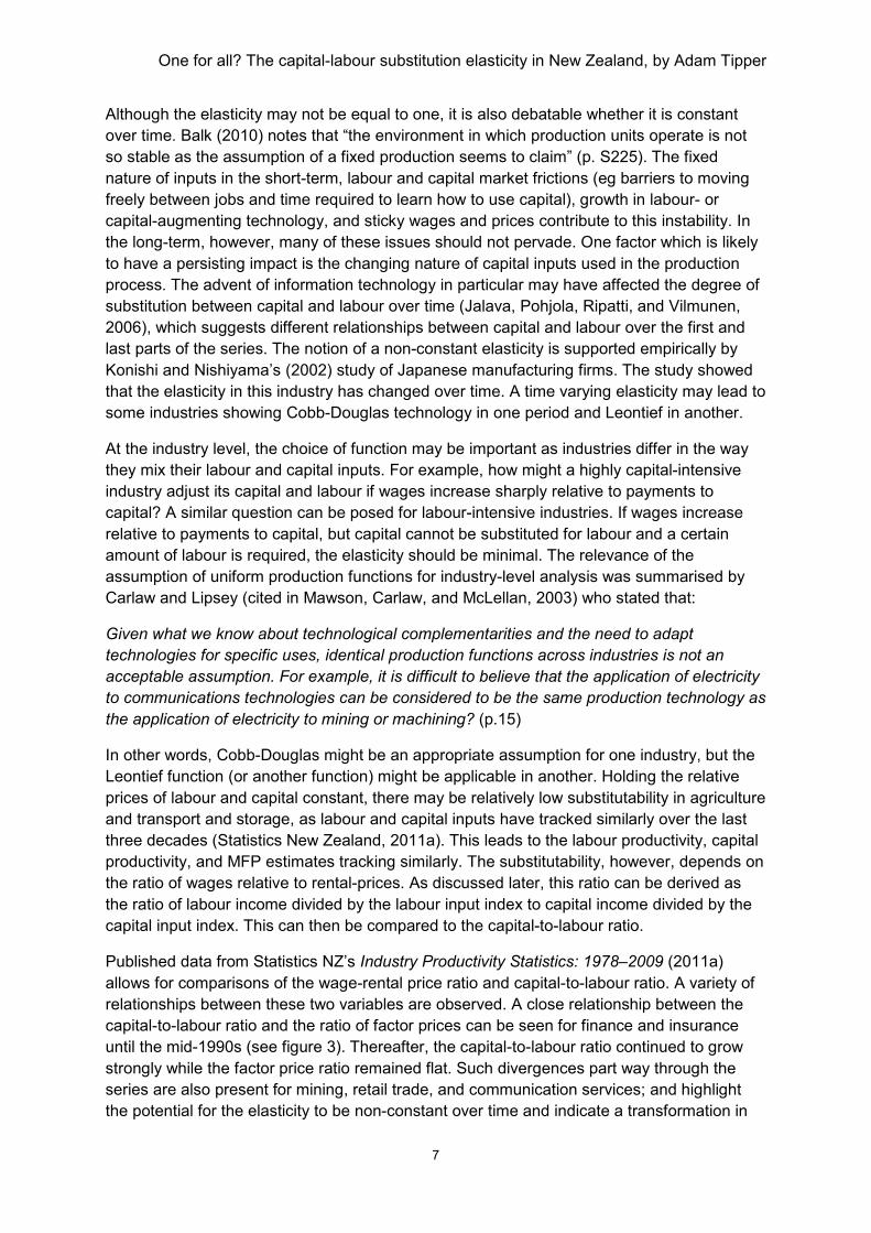
Published data from Statistics NZ’s Industry Productivity Statistics: 1978–2009 (2011a)
allows for comparisons of the wage-rental price ratio and capital-to-labour ratio. A variety of
relationships between these two variables are observed. A close relationship between the
capital-to-labour ratio and the ratio of factor prices can be seen for finance and insurance
until the mid-1990s (see figure 3). Thereafter, the capital-to-labour ratio continued to grow
strongly while the factor price ratio remained flat. Such divergences part way through the
series are also present for mining, retail trade, and communication services; and highlight
the potential for the elasticity to be non-constant over time and indicate a transformation in
One for all? The capital
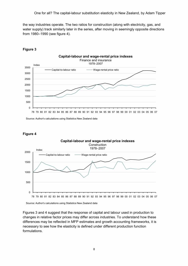
the way industries operate. The two ratios for
water supply) track similarly later in the
from 1980–1990 (see figure 4
Figure 3
Figure 4
Figures 3 and 4 suggest that the
changes in relative factor prices
differences may be reflected in
necessary to see how the elasticity
formulations.
0
500
1000
1500
2000
2500
3000
3500
78 79 80 81 82 83 84 85 86
Index
Capital
Capital-to-labour ratio
Source: Author's calculations using Statistics New Zealand data
0
500
1000
1500
2000
78 79 80 81 82 83 84 85 86
Index
Capital
Capital-to-labour ratio
Source: Author's calculations using Statistics New Zealand data
One for all? The capital-labour substitution elasticity in New Zealand, by Adam Tipper
8
The two ratios for construction (along with elec
later in the series, after moving in seemingly opposite directions
(see figure 4).
that the response of capital and labour used in production to
factor prices may differ across industries. To understand how these
differences may be reflected in MFP estimates and growth accounting frameworks
elasticity is defined under different production function
86 87 88 89 90 91 92 93 94 95 96 97 98 99 00 01 02
Capital-labour and wage-rental price indexesFinance and insurance
1978–2007
labour ratio Wage-rental price ratio
Statistics New Zealand data
86 87 88 89 90 91 92 93 94 95 96 97 98 99 00 01 02
Capital-labour and wage-rental price indexesConstruction1978–2007
labour ratio Wage-rental price ratio
Statistics New Zealand data
substitution elasticity in New Zealand, by Adam Tipper
onstruction (along with electricity, gas, and
after moving in seemingly opposite directions
capital and labour used in production to
across industries. To understand how these
estimates and growth accounting frameworks, it is
is defined under different production function
03 04 05 06 07
03 04 05 06 07
One for all? The capital-labour substitution elasticity in New Zealand, by Adam Tipper
9
Capital-labour substitution and production functions
There are a range of possible forms of the production function, with each form possessing
different mathematical properties and implications for the measurement of MFP.1 In the
econometric estimation of MFP, the choice of the production function depends on the
desired degree of flexibility (relative to the available data), whether the function is linear in
the parameters and satisfies the economic assumptions of homogeneity and monotonicty,
and the principle of parsimony (Coelli, Rao, O'Donnell, and Battese, (2005), p.211–212). The
last two of these criteria also apply to the index number approach to estimating MFP which is
used by Statistics NZ and other international statistical agencies.
Present in production functions are assumptions surrounding the elasticity between capital
and labour.2 The elasticity, denoted by �, for a production process with two inputs is defined as:
� � ���/����/�
/�/� (1)
Where � and are the quantities of labour and capital inputs, and � and � denote their respective marginal products (the change in output due to the change in the input). As
wages and rental-prices are assumed to be equal to the marginal revenue products of labour
and capital respectively, this definition depends on the assumption of perfect competition.
Where this assumption does not hold, estimates of the elasticity may be biased. Theories of
imperfect labour markets show that search frictions lead to an inherent divergence of wages
from the marginal revenue product, with the difference depending on the elasticity of labour
supply. Note also that equation 1 assumes that the elasticity is time invariant.
Cobb-Douglas To enable MFP to be calculated, the production function is assumed to be of the Cobb-
Douglas form. This approach has been the most frequently used in the productivity literature
(Miller, 2008), and has important properties (such as constant returns to scale and constant
factor such shares) and assumptions that facilitate productivity analysis. For example, the
Cobb-Douglas framework permits the rating forward of capital and labour income shares,
enabling estimates to be calculated even when current price national accounts data are
unavailable.3 The production function takes the form:
�� � ��������� ��� (2)
1 See appendix A for a discussion on production functions and productivity measurement. Further specifications include a quadratic form, normalised quadratic and the translog function. These forms are not discussed in this section as they do not yield exact assumptions regarding the capital-labour substitution elasticity and therefore do not present alternative hypotheses which can be tested in this framework. 2 Different forms of the production function also yield different elasticities of output with respect to inputs and therefore different marginal rates of technical substitution, which is related to the elasticity of substitution. This therefore has implications for computable general equilibrium models. 3An implication of the Cobb-Douglas approach is that factor shares are constant over time, meaning that these shares can assume a value factor income shares can be held constant even when current price data are not available.
One for all? The capital-labour substitution elasticity in New Zealand, by Adam Tipper
10
where �� = industry chain-volume value added ����� = a parameter that captures disembodied technical shifts over time, that is, for example, outward shifts of the production function allowing output to increase with a given
level of inputs (= MFP)
��= industry labour inputs ���= industry labour income share �= industry capital inputs ���=industry capital income share The use of income shares rests on the assumption of perfect competition, where economic
profits are zero, and value added is equal to the cost of labour and capital. Cost shares are
thus equal to income shares.
MFP is calculated residually, by dividing the output index by an index of total inputs:
����� � ��/���� ��� (3)
The elasticity under a Cobb-Douglas framework is equal to one, which implies that a unit of
capital is perfectly substitutable for a unit of labour. It is worth noting that this result is
independent of the assumption of constant returns to scale.
Leontief While the Cobb-Douglas production function assumes a unitary elasticity between capital
and labour, the Leontief production function assumes there is zero substitution between the
factors of production; that is, an increase in the amount of capital used by a firm or industry
is not matched by any corresponding change in labour following a change in relative prices.
The production function can be written as:
�� � ����� min ������, ��� �� (4)
In this case, output is maximised when there are fixed proportions of each input and one
(lowest cost) factor of production dominates total inputs. Therefore, when calculating MFP as
a residual, MFP (in a levels sense) will be greater as the elasticity tends to zero (Young,
1998).
Constant elasticity of substitution The production functions in equations 2 and 4 assume that the elasticity is either zero or
one. An alternative and more general specification is the Constant elasticity of substitution
(CES) production function, proposed by Arrow et al. (1961) who recognised that there were
varying degrees of substitutability between capital and labour inputs. The advantage of this
One for all? The capital-labour substitution elasticity in New Zealand, by Adam Tipper
11
function is that it has one less restrictive assumption by allowing the elasticity to take values
other than zero or one. The assumption of constant returns to scale is, however, still made.
In this case, output is related to inputs as follows:
�� � ����������� � ! �1 # ��� �� ���$/ � (5)
�0 & �� & 1; #1 & (� ) 0�
Where ��, �����, � , �� are defined as above, �� is a distribution parameter that reflects the relative factor shares, and (� is a parameter which determines the value of the elasticity. The elasticity can be derived as (see Chiang, 1984, p.428):
�� � $$* � (6)
In other words, the elasticity is a constant that can take on a value other than unity and
depends on the value of(�:
+#1 & (� & 0 (� � 00 & (� & ∞ - . /�� 0 1�� � 1�� & 1+
The constraints on (� require the elasticity to be non-negative. Other production functions can be seen as special cases of the CES function, depending on the value of (� . When (� = 0, the elasticity is equal to unity, and the CES production function approaches the Cobb-
Douglas function. This leads to a convex capital-labour relationship. However, the production
function is not defined when (� � 0 (as there will be division by 0), meaning that the CES and Cobb-Douglas functions are only approximate as (� tends towards 0. When (� � ∞, (ie there is no substitutability between the factors of production) the CES isoquant looks like the
Leontief isoquant (resulting in the familiar L shape relationship). When (� = 1, the production function will be linear (ie �� � ���������� ! �1 # ��� �� ) (see Varian, 1992, pp.19–20).
Implications for productivity
If MFP was to be calculated using the more general CES approach, then (using equation 4a
in appendix A and substituting in equation 6) the calculation becomes:
One for all? The capital-labour substitution elasticity in New Zealand, by Adam Tipper
12
234� � ����� � ��/������5��$�/5� ! �1 # ��� ��5��$�/5����5�/$�5�� (7)
While MFP is still derived as a residual, it can be seen that the calculation differs to that
under the Cobb-Douglas approach. In this instance, MFP depends on the elasticity between
capital and labour. MFP growth under a CES function will be less than that of a Cobb-
Douglas function when the elasticity is greater than unity. This is because, holding all else
equal, a higher elasticity leads to greater change in the total inputs index and therefore lower
change in MFP.
Labour and capital productivity estimates are defined under the CES model in the same
manner as the Cobb-Douglas function (ie the ratio of an index of outputs to respective
inputs). It is important to note that MFP estimates will still be between those for labour and
capital productivity as MFP is a weighted function of the two factors of production. This
implies that the form of the production function will have little empirical relevance for those
industries which have shown little difference in their labour and capital productivity growth
(eg accommodation, cafes, and restaurants, and transport and storage). Conversely, there
may be effects on MFP growth estimates for those industries which have shown diverging
labour and capital productivity (eg communication services, finance and insurance,
manufacturing).
The direction of the impact depends on the growth in labour and capital inputs. As the
elasticity approaches zero (the Leontief function), total inputs track towards the input which
has shown the slowest growth (ref. equation 4). Lower elasticities imply slower growth in
total inputs, and thus higher MFP growth. This, however, assumes that the parameter � is constant. If this is non-constant, then there may be offsetting effects on the total input and
MFP indexes.
Regardless of the size of the quantitative impact on estimating MFP, the form of the
production function has implications for the interpretation of MFP growth. As constructed by
Statistics NZ, MFP is a valid measure of technological change when the production function
is of the Cobb-Douglas form. Under a CES model, MFP reflects technological change as
well as the constraints of adjusting production to relative factor prices.
The choice of production function also has implications for growth accounting for both output
and labour productivity. As labour productivity is calculated as a ratio of output to labour
input and MFP depends on the elasticity, the contribution of capital deepening must differ
when the elasticity is not equal to unity. In other words, the weight used to calculate the
contribution of capital deepening will not be equal to capital’s share of income. Instead it will
reflect the responsiveness of capital and labour to relative factor prices. Under a CES
approach, the contributions of capital and labour inputs to output growth capture the degree
to which inputs are substituted according to relative prices as well as factor income shares.
Using equations 5 and 6, output can be decomposed as follows:
6 ln �� � 6 ln ����� # 5�$�5� 6 ln�����5��$�/5� !�1 # ��� �5��$/5�� (8)
One for all? The capital-labour substitution elasticity in New Zealand, by Adam Tipper
13
The core contributions are the same as those under the Cobb-Douglas function (MFP,
capital input, and labour input), but the weights depend on the elasticity. From equation 8, it
can be observed that the elasticity will have an impact on growth rates. If this formulation
was extended to allow the elasticity to vary over time, then there would be a further effect on
growth.
Empirical analysis
To understand whether the choice of production function may have an impact on the
estimate of MFP, an estimate for the value of � is required. An econometric approach is adopted for two reasons: first, indications of statistical significance are required, and this
cannot be obtained by direct computation; and second, the dynamics of capital accumulation
need to be taken into account as quantities in one period may depend on their prior values.
Balistreri et al. (2003) outline an econometric framework that can be applied to the available
New Zealand data. Maximising the CES production function, subject to the budget
constraint, yields the following specification:
ln ���� � ���8 9�$�9� ! ���8 �� (9)
The left hand side of the equation is the logarithm of the capital-to-labour ratio, and the right
hand side is equal to a constant plus the logarithm of the wage-rental price ratio multiplied by
the elasticity. Equation 9 can be rearranged so that it can be estimated by ordinary least
squares:
ln :� �;�! <� ln =� ! >� (10)
The first term in equation 9, :�, is the capital-to-labour ratio. The wage-rent ratio is denoted by =�. The <� term is the key parameter to be estimated and >�? is an identically and independently distributed error term. The constant term ;� reflects the assumption that the factor cost ratio is constant “if the firm production function is Cobb-Douglas with labour and
capital as inputs, and firms cost minimize facing competitive factor markets” (Raval, 2011,
p.12).
Balistreri et al. (2003) note that a simple linear regression may not provide reliable estimates
as the role of dynamics between capital and labour need to be considered, and suggest
three specifications to account for this. The first model employed in this analysis is based on
equation 10, but includes a lagged dependent variable as an independent variable (leading
to a first order autoregressive model, denoted hereafter by AR1):
One for all? The capital-labour substitution elasticity in New Zealand, by Adam Tipper
14
ln :�? �;�! <$� ln =�? ! <@� ln :�?�$ ! ��� ! >�? (11)
Lags are important for understanding the evolution of the capital-labour ratio due to inertia,
technological factors, imperfect information, or institutional (contractual) effects (Gujarati,
1995, pp.589–590). The choice of lag length is important, as the same structure may not be
applicable to all industries. If industry-specific lags are not taken account of, then coefficients
may be biased. The use of lagged terms means that long-run as well as short-run elasticity
estimates can be derived. The short-run elasticity is <$� .The long-run elasticity takes into account the effect of contemporaneous and lagged variables and is calculated as <$�/�1 #<@�� where <@� ) 1. Equation 11 deviates from the approach of Balistreri et al. (2003) by including a time trend.
This is to account for any factors other than prices and lagged dependency that may be
affecting the capital-to-labour ratio, such as labour (Harrod-neutral) or capital (Solow-neutral)
augmenting technological change. Jalava et al. (2006) highlight the importance of including a
time trend in order to control for possible bias from mis-specification of the nature of
technological change. Capital augmenting technological change has likely occurred since
the evolution in information and communication technology. Consider figure 1, where capital-
augmenting technological change leads to a pivoted outward shift of the production
possibility frontier and capital production functions. Under perfect competition, the marginal
product of capital equals the rental price thus changing the slope of the budget constraint.
The capital-to-labour isoquant will flatten as more output can be produced by less capital.
These effects can be captured by a time trend. Econometrically, this implies that the capital-
to-labour ratio is trend stationary. In economic terms, this means that no assumptions
regarding the nature of technological change are made.
The second model is based on first differences of the dependent and independent variables:
∆ln :�? �;�! <$�∆ ln =�? ! ��� ! >�? (12)
where ∆ ln =�? � ln =�? # ln =�?�$ denotes the first difference. This specification is preferred if the capital-to-labour and wage-rental price ratios are non stationary (ie the variances depend
on time). If the ratios are non-stationary then the AR1 regression is ‘spurious’ and the
coefficients and derived elasticities are meaningless. As there are no lagged terms in this
specification, only the short-run estimate is derived (and is equal to <$�). Balistreri et al. (2003) also employ a single equation error correction model (hereafter ECM) to determine
the elasticity. It is based on first differences with lagged dependent and independent
variables as regressors:
∆ln :�? �;�! <$�∆ ln =�? ! <@� ln :�?�$ ! <B� ln =�?�$ !��� ! >�? (13)
In this model, the short-run elasticity is again <$� but the long-run elasticity is #<B�/<@� where <@� ) 0. This model is more appropriate when the variables are non-stationary and when an
One for all? The capital-labour substitution elasticity in New Zealand, by Adam Tipper
15
indication of the long-run elasticity is required (as is the case here). It allows for the
divergence of short-run deviations from long-run equilibrium to be assessed. For some
industries, a second difference model is more appropriate or the time trend is not required.
Dickey-Fuller tests were used to provide guidance on the degree of differencing and use of
trends. Where this is the case, the ECM is modified accordingly.
A further constraint to estimation is that the elasticity must be positive. A negative elasticity
has no economic interpretation: “it implies a decline in the availability of one input can be
made up by a decline in the availability of other factors.” (World Bank, 2006, p.117).
Negative elasticities have been found in some studies (see the results of Balistreri et al.,
2003 and Raval, 2011) and can arise when the dynamic structure of an industry is not fully
considered (eg when too few lags are specified in the regression equation). Economic theory
therefore needs to be considered alongside the results of statistical tests, and further
investigation is warranted where this condition is violated.
Data
Data were required for labour and capital volumes to construct the dependent capital-to-
labour ratio variable, and wage and rental prices were required to calculate the independent
wage-rental price ratio.4 The wage and rental price variables are expressed in nominal
terms, consistent with the approach of Balistreri et al. (2003). Labour income includes
compensation of employees, net taxes on production attributable to labour income, and the
labour income of working proprietors. Capital income is the sum of gross operating surplus
(adjusted for the labour income of working proprietors) and net taxes on production
attributable to capital.5
The capital-to-labour ratio for a given industry was defined as the ratio of an index of capital
input to an index of labour input. The wage rate was calculated as labour income divided by
the labour input index. Rental prices were calculated in a similar manner, by dividing capital
income by the capital input index. The wage rental-price ratio is then derived as the ratio of
these two ratios.6 The wage and rental prices can be considered implicit (rather than explicit)
prices. Rental price calculations in particular may not match those underlying productivity
data as the implicit approach assumes an endogenous rate of return (such that user costs
completely exhaust capital income). Statistics NZ, however, assumes an exogenous rate of
return (set at 4 percent). Therefore, there may be difference between explicit rental prices as
used to calculate MFP and the implicit series used in this analysis.
Labour input for each industry is measured as a sum of industry hours paid with the data
sourced from a variety of labour surveys such as the Linked-Employee-Employer Dataset,
Household Labour Force Survey, Quarterly Employment Survey, and the Business
Demography Database. To measure the flow of capital services, the perpetual inventory
method is used to derive the productive capital stock and supplemented with estimates of
4 Unrounded data were used in this analysis. 5 See sections 3.5.2 and 4.6 in Statistics New Zealand (2011b) Productivity statistics: Sources and methods for further information on the calculation of labour and capital income, respectively. 6 As stated by Coelli et al (2005), substitution elasticities are invariant to the units of measurement because they depend on first order conditions. This implies that labour and capital input indexes can be used instead of actual values.
One for all? The capital-labour substitution elasticity in New Zealand, by Adam Tipper
16
land and inventories to create capital inputs. Measured sector (and other aggregated) capital
and labour series are weighted together using their respective income shares.7
The measured sector covers ANZSIC96 industries A-K, LA, LC, PA, and QA (see appendix
B). However, property and business services, and personal and other community services
are included in the measured sector from 1996. This means that estimating the elasticity
from 1978 to 2007 is problematic as the industry composition changes over time. The former
measured sector (A-K and P) has consistent industry coverage from 1978 to 2007 and is
therefore preferable.
For the industry-level analysis, property and business services, cultural and recreational
services, and personal and other community services were excluded as their productivity
time series only begins in 1996, and longer-time series were required to obtain reliable
estimates for the elasticity at the industry level. This meant 20 industries were included in the
model; nine of these were the manufacturing sub-industries. In 2007, the measured sector
covered 80 percent of the economy in terms of current price gross domestic product (GDP).
Data were only available until 2007 as this is the last year for which current price estimates
of GDP by industry are available.
Results
The previous discussion raised three issues that are worth exploring empirically. First, an
estimate of the elasticity is required along with a statistical test to determine whether the
data supports a Cobb-Douglas, Leontief, or CES production function. Second, the
application of Cobb-Douglas across different levels of aggregation needs to be assessed.
This exploration allows us to see whether aggregating production functions of the same
functional form is the same as a defining a separate aggregator. Third, an assessment of the
applicability of Cobb-Douglas across the same level of aggregation is required as it can be
expected that not all industries respond to changing factor prices to the same degree or do
so at the same pace.
Two null hypotheses were tested for both the short and long-run elasticity. The first was that
the elasticity was equal to unity. Rejecting this null means the data does not provide
evidence for the Cobb-Douglas function. The second hypothesis was that the elasticity was
equal to zero. In this case, rejection means that the data does not provide evidence for the
Leontief specification. All tests were performed at the 95 percent confidence level.
Regression results are presented in appendix C.
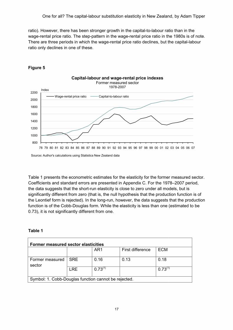
Measured sector elasticities Figure 5 shows the trends in the capital-to-labour ratio and wage-rental price ratio over the
series for the measured sector. Both ratios have trended upwards over time, implying that
payments to labour have risen at a higher rate than payments to capital and that there is
more capital available per worker (consistent with the trend in the chained capital-to-labour
7 Further details on the data sources and construction of the series can be found in Productivity statistics: Sources and methods, Statistics New Zealand (2011b).
One for all? The capital
ratio). However, there has been stronger growth in
wage-rental price ratio. The step
There are three periods in which the wage
ratio only declines in one of these
Figure 5
Table 1 presents the econometric estimates for the elasticity for the former measured sector
Coefficients and standard errors are presented in Appendix C. For the 1978
the data suggests that the short
significantly different from zero
the Leontief form is rejected).
function is of the Cobb-Douglas
0.73), it is not significantly different from one.
Table 1
Former measured sector elasticities
Former measured
sector
SRE
LRE
Symbol: 1. Cobb-Douglas function cannot be rejected
800
1000
1200
1400
1600
1800
2000
2200
78 79 80 81 82 83 84 85 86
Index
Capital
Wage-rental price ratio
Source: Author's calculations using Statistics New Zealand data
One for all? The capital-labour substitution elasticity in New Zealand, by Adam Tipper
17
re has been stronger growth in the capital-to-labour ratio
The step-pattern in the wage-rental price ratio in the 1980s is of n
re are three periods in which the wage-rental price ratio declines, but the
only declines in one of these.
presents the econometric estimates for the elasticity for the former measured sector
and standard errors are presented in Appendix C. For the 1978
the data suggests that the short-run elasticity is close to zero under all model
significantly different from zero (that is, the null hypothesis that the production func
rejected). In the long-run, however, the data suggests that the production
Douglas form. While the elasticity is less than one (estimated to be
0.73), it is not significantly different from one.
Former measured sector elasticities
AR1 First difference ECM
0.16 0.13 0.18
0.73(1) 0.73(1)
Douglas function cannot be rejected.
86 87 88 89 90 91 92 93 94 95 96 97 98 99 00 01 02
Capital-labour and wage-rental price indexesFormer measured sector
1978-2007
rental price ratio Capital-to-labour ratio
Statistics New Zealand data
substitution elasticity in New Zealand, by Adam Tipper
labour ratio than in the
ratio in the 1980s is of note.
the capital-labour
presents the econometric estimates for the elasticity for the former measured sector.
and standard errors are presented in Appendix C. For the 1978–2007 period,
models, but is
(that is, the null hypothesis that the production function is of
data suggests that the production
While the elasticity is less than one (estimated to be
(1)
03 04 05 06 07

One for all? The capital-labour substitution elasticity in New Zealand, by Adam Tipper
18
While the short-run estimate under the AR1 model is low (but still significantly different from
zero) the long-run elasticity shows a much stronger relationship between the capital-to-
labour ratio and the wage-rental price ratio. This highlights the role of lags in the relationship
in the formation of the capital-to-labour ratio. Across models, the short-run estimates are
broadly consistent and the AR1 model and ECM produce identical values for the elasticity.
The capital-to-labour ratio and the wage-rental price ratio, however, are both non-stationary
and cointegrated. Dickey-Fuller tests were performed to test whether the capital-to-labour
ratio and wage-rental-price ratio for each sector and industry has a unit root. Where
evidence for a unit root can be found, the first difference model is more appropriate. If the
unit root hypothesis is rejected then the AR1 model is appropriate. The first difference model
is preferred to the AR1 model as the Dickey-Fuller tests indicate that both series are non-
stationary at the former measured sector level. However, the Phillips-Ouliaris test indicates
that the series are cointegrated, implying the ECM provides additional information on the
long-run response.
Jarque-Bera tests indicate that the data are not normally distributed, and both the Durbin-
Watson statistic (applied to the first difference model and ECM) and the Durbin h test
(applied to the AR1 model) indicate that autocorrelation is present. This may inflate the
standard error, leading to incorrect conclusions regarding significance, and overinflate the R2
value. The R2 values of 0.99 under the AR1 model are much greater than those of the first
difference model or ECM (0.19 and 0.29, respectively). However, the presence of
autocorrelation does not bias the estimates of the coefficients.
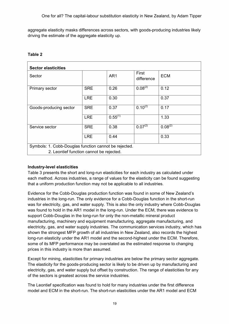
Sector–level elasticities Elasticities of capital-labour substitution were calculated using productivity estimates for the
primary, goods-producing, and service sectors. Differences in the elasticity can be expected
across sectors for a number of reasons: each sector uses different types of assets, the
service sector is more labour-intensive, and capital-deepening has been more pronounced in
the goods-producing sector.8
As shown in table 2, the elasticity varies across sectors. The first difference model suggests
similar elasticities for all sectors, and that the Leontief production function holds in the short-
run. However, the Leontief function is rejected in the short-run under the AR1 model and the
ECM (except for services). Some evidence for the Cobb-Douglas hypothesis could be found
in the long-run for the goods-producing sector. The ECM for the goods-producing sector
uses second difference with two year lags and no time trend. This means that the effect of
an increase in the wage-rental price ratio takes longer to impact on the capital-to-labour ratio
in the goods-producing sector than in the primary or service sectors. The Philips-Ouliaris
tests again indicate that the ECM is preferable to the first difference model. Note that the
service sector includes additional industries from 1996 which may bias the estimates.9 The
8 The primary sector includes the agriculture, forestry, fishing, and mining industries. The goods-producing sector includes manufacturing, electricity, gas, and water supply, and construction. The service sector includes the following industries from 1978: wholesale trade; retail trade; accommodation, cafes, and restaurants; transport and storage; communication services; finance and insurance; and cultural and recreational services. Business services, property services, and personal and other community services are included in the service sector from 1996. 9 Ideally, the service sector would exclude business services, property services, and personal and other community services to obtain consistent industry coverage. Preliminary analysis using measured sector data, however, showed that the long-run elasticity differed from the former measured sector elasticity by only 0.01. This suggests minimal bias in the service sector estimate.
One for all? The capital-labour substitution elasticity in New Zealand, by Adam Tipper
19
aggregate elasticity masks differences across sectors, with goods-producing industries likely
driving the estimate of the aggregate elasticity up.
Table 2
Sector elasticities
Sector
AR1 First
difference ECM
Primary sector SRE 0.26 0.08(2) 0.12
LRE 0.30 0.37
Goods-producing sector SRE 0.37 0.10(2) 0.17
LRE 0.55(1) 1.33
Service sector SRE 0.38 0.07(2) 0.08(2)
LRE 0.44 0.33
Symbols: 1. Cobb-Douglas function cannot be rejected.
2. Leontief function cannot be rejected.
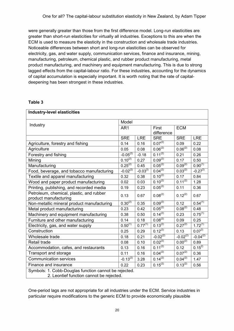
Industry-level elasticities
Table 3 presents the short and long-run elasticities for each industry as calculated under
each method. Across industries, a range of values for the elasticity can be found suggesting
that a uniform production function may not be applicable to all industries.
Evidence for the Cobb-Douglas production function was found in some of New Zealand’s
industries in the long-run. The only evidence for a Cobb-Douglas function in the short-run
was for electricity, gas, and water supply. This is also the only industry where Cobb-Douglas
was found to hold in the AR1 model in the long-run. Under the ECM, there was evidence to
support Cobb-Douglas in the long-run for only the non-metallic mineral product
manufacturing, machinery and equipment manufacturing, aggregate manufacturing, and
electricity, gas, and water supply industries. The communication services industry, which has
shown the strongest MFP growth of all industries in New Zealand, also records the highest
long-run elasticity under the AR1 model and the second-highest under the ECM. Therefore,
some of its MFP performance may be overstated as the estimated response to changing
prices in this industry is more than assumed.
Except for mining, elasticities for primary industries are below the primary sector aggregate.
The elasticity for the goods-producing sector is likely to be driven up by manufacturing and
electricity, gas, and water supply but offset by construction. The range of elasticities for any
of the sectors is greatest across the service industries.
The Leontief specification was found to hold for many industries under the first difference
model and ECM in the short-run. The short-run elasticities under the AR1 model and ECM
One for all? The capital-labour substitution elasticity in New Zealand, by Adam Tipper
20
were generally greater than those from the first difference model. Long-run elasticities are
greater than short-run elasticities for virtually all industries. Exceptions to this are when the
ECM is used to measure the elasticity in the construction and wholesale trade industries.
Noticeable differences between short and long-run elasticities can be observed for
electricity, gas, and water supply, communication services, finance and insurance, mining,
manufacturing, petroleum, chemical plastic, and rubber product manufacturing, metal
product manufacturing, and machinery and equipment manufacturing. This is due to strong
lagged effects from the capital-labour ratio. For these industries, accounting for the dynamics
of capital accumulation is especially important. It is worth noting that the rate of capital-
deepening has been strongest in these industries.
Table 3
One-period lags are not appropriate for all industries under the ECM. Service industries in
particular require modifications to the generic ECM to provide economically plausible
Industry-level elasticities
Industry
Model
AR1 First difference
ECM
SRE LRE SRE SRE LRE
Agriculture, forestry and fishing 0.14 0.16 0.07(2) 0.09 0.22
Agriculture 0.05 0.08 0.06(2) 0.06
(2) 0.08
Forestry and fishing -0.05(2) -0.18 0.11
(2) 0.21 0.26
Mining 0.10(2) 0.27 0.09
(2) 0.17 0.50
Manufacturing 0.25(2) 0.45 0.05
(2) 0.09
(2) 0.90
(1)
Food, beverage, and tobacco manufacturing -0.02(2) -0.03
2) 0.04
(2) 0.03
(2) -0.27
2)
Textile and apparel manufacturing 0.32 0.38 0.10(2) 0.17 0.84
Wood and paper product manufacturing 0.02 0.03 0.10(2) 0.11
(2) 1.28
Printing, publishing, and recorded media 0.19 0.23 0.05(2) 0.11 0.36
Petroleum, chemical, plastic, and rubber product manufacturing
0.13 0.67 0.08(2) 0.12
(2) 0.67
Non-metallic mineral product manufacturing 0.30(2) 0.35 0.09
(2) 0.12 0.54
(1)
Metal product manufacturing 0.23 0.42 0.05(2) 0.08
(2) 0.48
Machinery and equipment manufacturing 0.38 0.50 0.14(2) 0.23 0.75
(1)
Furniture and other manufacturing 0.14 0.18 0.08(2) 0.09 0.25
Electricity, gas, and water supply 0.50(1) 0.77
(1) 0.13
(2) 0.27
(2) 1.72
(1)
Construction 0.25 0.29 0.12(2) 0.13 0.07
2)
Wholesale trade 0.18 0.21 -0.02(2) -0.02
(2) -0.04
(2)
Retail trade 0.08 0.10 0.02(2) 0.00
(2) 0.89
Accommodation, cafes, and restaurants 0.13 0.16 0.11(2) 0.12 0.15
2)
Transport and storage 0.11 0.16 0.04(2) 0.07
(2) 0.36
Communication services -0.13(2) 3.28 0.14
(2) 0.04
(2) 1.47
Finance and insurance 0.22 0.23 0.15(2) 0.13
(2) 0.56
Symbols: 1. Cobb-Douglas function cannot be rejected. 2. Leontief function cannot be rejected.

One for all? The capital-labour substitution elasticity in New Zealand, by Adam Tipper
21
estimates. An ECM with second differences, two year lags and no time trend was used for
forestry and fishing and finance and insurance. The time trend was omitted for wood and
paper product manufacturing, wholesale trade, and retail trade. Mining is a peculiar case.
Applying a standard ECM to this industry, using any lag length and differences up to three
years, results in large negative elasticities (which has no economic meaning). Diminishing
marginal productivity of labour is pronounced in this industry. The greatest change in output
occurs once extraction begins and, holding labour input constant, there is little scope to
increase extraction in subsequent years. This implies an adaptive expectations model where
current investment depends on the observed realisations of prior investments. The capital-
to-labour ratio and wage-rental price are thus constructed by comparing the current capital
input in production and associated income with a two-year lag of labour input and income.
This results in a positive elasticity for mining.
In most industries and models, the elasticity is less than unity. This concurs with
expectations as the estimates are between the values proposed by the Leontief and Cobb-
Douglas functions. Assuming rental prices and capital are constant, an elasticity less than
unity implies that a wage increase has a less than proportionate effect on labour demand. In
other words, it is not as easy for most industries to shift between capital and labour as the
Cobb-Douglas assumption implies. Only in a few cases were the elasticities above unity.
Some negative elasticities were also found. However, the Leontief function cannot be
rejected in most of these cases and a value of zero can be assumed for these industries.
The negative elasticity for the food, beverage, and tobacco manufacturing industry persists
under any specification. Recalling the discussion on implications of different elasticities for
MFP estimation, these results suggest that MFP may be biased downwards. Therefore MFP
may be contributing more to output growth than expected, and labour and capital less than
currently estimated. CES production functions with lower elasticity values are applicable for
most industries.
The AR1 models have strong explanatory power, with R2 values of approximately 90 percent
observed for most industries. The importance of accounting for deviations from equilibrium is
highlighted by the weak explanatory power of the first difference models and the higher R2
values from the ECM. The high AR1 R2 values, however, reflect the presence of
autocorrelation. Durbin-Watson h tests for the AR1 model suggest autocorrelation is present
in all industries except printing, publishing, and recorded media and furniture and other
manufacturing at the 95 percent confidence level. Durbin-Watson statistics for the first
difference models, however, show less evidence of autocorrelation.10
The first difference model results are generally preferred over the AR1 model, due to the
results of the Dickey-Fuller tests. The Phillips Ouliaris test, however, indicates that the ECM
is preferable for a number of industries. Appendix C provides further information on the
various tests applied to the industry-level data. Industry-specific considerations were made
for the lag structure in the ECM, to capture feedback effects as accurately as possible. The
choice of lag structure and inclusion of time trend has a significant impact on the estimates
under the ECM. The AR1 and first difference was applied uniformly to all industries: variants
of these models were examined but had no major impact on the results.
10Jarque-Bera tests indicate the error terms are normally distributed for all industries except petroleum, chemical,
plastic, and rubber product manufacturing and furniture and other manufacturing.
One for all? The capital
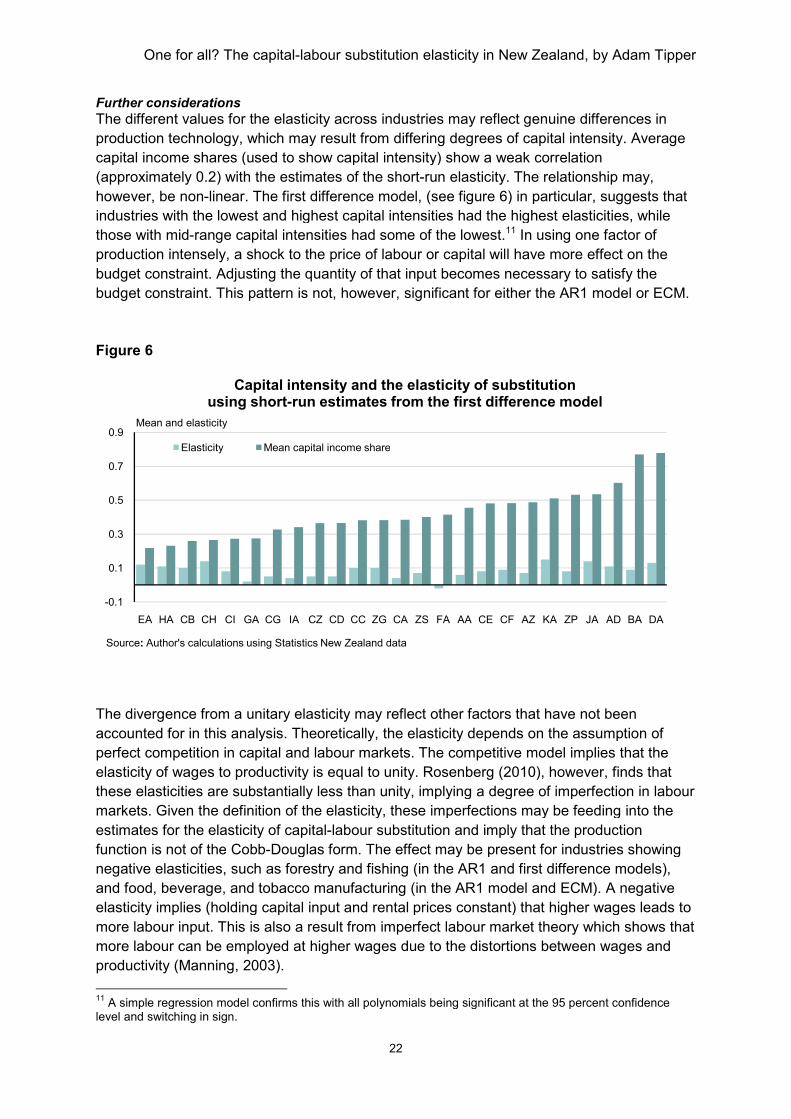
Further considerations
The different values for the elasticity across industries may reflect genuine differences in
production technology, which may result from
capital income shares (used to show capital intensity) show a
(approximately 0.2) with the estimates of the
however, be non-linear. The first difference
industries with the lowest and highest capital intensities had the highest elasticities, while
those with mid-range capital intensities had some of the lowest.
production intensely, a shock to the price of labour or capital will have more effe
budget constraint. Adjusting the quantity of that input becomes necessary to satisfy the
budget constraint. This pattern is
Figure 6
The divergence from a unitary elasticity may reflect other factors that have not been
accounted for in this analysis.
perfect competition in capital and labour markets. The competitive model
elasticity of wages to productivity is equal to unity. Rosenberg (2010), however, finds that
these elasticities are substantially less than unity, implying a degree of imperfection in labour
markets. Given the definition of the elasticity,
estimates for the elasticity of capital
function is not of the Cobb-Doug
negative elasticities, such as forestry and fishing
and food, beverage, and tobacco manufacturing
elasticity implies (holding capital input and rental prices constant) that higher wages leads to
more labour input. This is also a result from imperfect labour market theory which shows that
more labour can be employed at higher wages due to the distortions between wages and
productivity (Manning, 2003).
11 A simple regression model confirms this with all polynomials being significant at the 95 percent
level and switching in sign.
-0.1
0.1
0.3
0.5
0.7
0.9
EA HA CB CH CI GA CG
Mean and elasticity
Capital intensity and the elasticity of substitutionusing short
Elasticity Mean capital income share
Source: Author's calculations using Statistics New Zealand data
One for all? The capital-labour substitution elasticity in New Zealand, by Adam Tipper
22
The different values for the elasticity across industries may reflect genuine differences in
production technology, which may result from differing degrees of capital intensity.
capital income shares (used to show capital intensity) show a weak correlation
with the estimates of the short-run elasticity. The relationship may,
first difference model, (see figure 6) in particular
industries with the lowest and highest capital intensities had the highest elasticities, while
range capital intensities had some of the lowest.11 In using one factor of
k to the price of labour or capital will have more effe
djusting the quantity of that input becomes necessary to satisfy the
This pattern is not, however, significant for either the AR1
The divergence from a unitary elasticity may reflect other factors that have not been
accounted for in this analysis. Theoretically, the elasticity depends on the assumption of
perfect competition in capital and labour markets. The competitive model implies that the
elasticity of wages to productivity is equal to unity. Rosenberg (2010), however, finds that
these elasticities are substantially less than unity, implying a degree of imperfection in labour
markets. Given the definition of the elasticity, these imperfections may be feeding into the
estimates for the elasticity of capital-labour substitution and imply that the production
Douglas form. The effect may be present for industries showing
forestry and fishing (in the AR1 and first difference models)
and tobacco manufacturing (in the AR1 model and ECM)
elasticity implies (holding capital input and rental prices constant) that higher wages leads to
labour input. This is also a result from imperfect labour market theory which shows that
more labour can be employed at higher wages due to the distortions between wages and
A simple regression model confirms this with all polynomials being significant at the 95 percent
IA CZ CD CC ZG CA ZS FA AA CE CF AZ KA ZP
Capital intensity and the elasticity of substitutionusing short-run estimates from the first difference model
Mean capital income share
Statistics New Zealand data
substitution elasticity in New Zealand, by Adam Tipper
The different values for the elasticity across industries may reflect genuine differences in
of capital intensity. Average
correlation
. The relationship may,
) in particular, suggests that
industries with the lowest and highest capital intensities had the highest elasticities, while
In using one factor of
k to the price of labour or capital will have more effect on the
djusting the quantity of that input becomes necessary to satisfy the
AR1 model or ECM.
The divergence from a unitary elasticity may reflect other factors that have not been
depends on the assumption of
implies that the
elasticity of wages to productivity is equal to unity. Rosenberg (2010), however, finds that
these elasticities are substantially less than unity, implying a degree of imperfection in labour
these imperfections may be feeding into the
labour substitution and imply that the production
The effect may be present for industries showing
(in the AR1 and first difference models),
(in the AR1 model and ECM). A negative
elasticity implies (holding capital input and rental prices constant) that higher wages leads to
labour input. This is also a result from imperfect labour market theory which shows that
more labour can be employed at higher wages due to the distortions between wages and
A simple regression model confirms this with all polynomials being significant at the 95 percent confidence
ZP JA AD BA DA
Capital intensity and the elasticity of substitutionrun estimates from the first difference model
One for all? The capital-labour substitution elasticity in New Zealand, by Adam Tipper
23
A further potential explanation for the divergence from a unitary substitution lies also in the
utilisation of inputs (Felipe and McCombie, 2005). The calculation of capital inputs assumes
that the rate of capacity utilisation is constant. As capacity utilisation adjustment involves
adjusting capital inputs, but capital income is held constant, the estimated elasticity should
change. Without adjustment, a strong increase in the wage-rental price ratio may have little
effect on the capital-to-labour ratio as the effect of firms opting to increase the utilisation of
their existing inputs rather than invest in additional capital or labour will not be captured. This
also implies that industries may not be operating on their production possibility frontier,
which is an assumption required for estimating the elasticity.
It might be expected that the industry-level elasticities are affected by the leasing of assets.
Estimates of the volume of the productive capital stock (used to derive the flow of capital
services) are based on ownership of assets rather than use. The rental price (calculated as
capital income over capital inputs) for an industry which rents its assets from other
industries, may include income derived from these assets. The rent payable, however, is
included in intermediate consumption. Under a perfectly competitive market with no
transaction costs, the income from the rented asset should equal the rent paid (as economic
profits are zero). In this case, the rental price would only reflect assets owned and the
coverage of the capital-labour ratio would be consistent with the wage-rental price ratio.
However, where market imperfections exist, such that rents differ from generated income,
the wage-rental price is not directly comparable with the capital-labour ratio and the elasticity
may not reflect the actual substitution which occurs. Where this is the case, aggregated
estimates are preferable to industry estimates and industry estimates can only be interpreted
as elasticities for assets owned. Data on rented assets are unfortunately not available to
provide context for that scenario. Controlling for the lagged capital-to-labour ratio may
account for that scenario to some extent. In the long-run, as rent seeking behaviour (and
other imperfections) diminish, ownership of capital becomes more economically rational and
the capital-to-labour ratio adjusts accordingly.
In conclusion Under an economic framework, estimation of MFP growth requires a production function with
associated assumptions or estimates for the elasticity between capital and labour. This
paper has sought to estimate these elasticities using data from Statistics NZ’s productivity
series in an econometric framework. Three econometric methods were employed to
determine the elasticity: a first order AR1 model, a first difference model, and an ECM. Each
of these models is advantageous to varying degrees, depending on the time series nature of
the capital-to-labour and wage-rental price ratios. In specifying the dynamics of capital
accumulation, we can derive estimates of both short- and long-run elasticities for the former
measured sector and each industry in the analysis.
The data suggests that a Cobb-Douglas form of the constant elasticity production function is
appropriate at the aggregate level in New Zealand in the long-run. At the industry-level, the
evidence suggests that a constant elasticity production function with varying elasticities
across industries is appropriate. These findings align with those of Balistreri et al. (2003) in
that a range of estimates for the elasticity can be found across industries. The hypothesis
that there is one production function for all cannot be supported. The findings presented in

One for all? The capital-labour substitution elasticity in New Zealand, by Adam Tipper
24
this paper show that the Leontief function is more applicable in the short-run but not the
long-run. This concurs with Sneessens and Dreze (1986) who find that the impact of
changing factor costs on optimal technical coefficients occurs predominantly after one year.
This paper has also shed some light on the dynamics of capital deepening in the New
Zealand economy. Growth in the capital-to-labour ratio depends strongly on previous growth
and, to a lesser extent, on changes in relative factor prices. The effects, however, depend on
the specification of the econometric model as different industries are susceptible to feedback
effects to varying degrees.
In interpreting the implications of this analysis, a number of caveats need to be borne in
mind. In terms of the econometric methods employed: i) the choice of econometric
specification is important, and may lead to widely different results, and ii) the sample sizes
for the regressions are small (due to the limited time series that are available) meaning that
the estimates may be sensitive to revisions or additional years of data. While attempts have
been made to examine the dynamic structure for each industry, the results are often
sensitive to the choice of lag length or degree of differencing.
Re-calculating industry-level productivity for those industries showing an elasticity
significantly different to unity is not straight-forward. The requirements for estimating reliable
elasticities are strong due to the number of econometric issues. Using the elasticities to
estimate MFP may introduce more bias into the model than is already present. This is
especially true if the elasticity is dependent on time or if outliers are significantly influencing
the results. The use of annual data may also lead to an underestimate of the true elasticity
(Chirinko et al., 2004, p.3) as the long-run is defined over too short a time frame. Further
consideration needs to be made regarding the calculation of rental prices. Rental prices can
be calculated directly using the underlying productive capital stock data, rather than deriving
an implicit rental price by dividing capital income by capital input. Differences between the
two can be expected, given the use of an exogenous rate of return used in the user cost
equation. This means that capital income may not equal rental prices multiplied by the
productive capital stock. More importantly, the Cobb-Douglas approach is the international
standard. Statistics NZ’s methods for calculating MFP are being compiled in accordance with
best practice and altering the assumptions regarding the process of production would affect
international comparability.
Productivity measurement uses a variety of data sources, each of which may be subject to a
degree of sampling and non-sampling error. However, the deviation of additional
assumptions required for productivity measurement from expectations may also be a source
of bias. Any mis-specification of these assumptions will be captured in the MFP residual.
This analysis suggests that the form of the production function may be generating some bias
in the MFP residual, and is likely biasing current estimates downwards. While the
quantitative impact may be small (as MFP growth will still be between labour and capital
productivity) there are implications for what MFP estimates mean; MFP does not solely
reflect technological change, it also reflects the way inputs are employed and their flexibility
to market prices.
One for all? The capital-labour substitution elasticity in New Zealand, by Adam Tipper
25
References
Arrow, KJ, Chenery, HB, Minhas BS, and Solow RM (1961). Capital-labor substitution and
economic efficiency. The Review of Economics and Statistics, 43(3), pp.225–250.
Balistreri, EJ, McDaniel, CA, and Wong, EV (2003). An estimation of US industry-level
capital-labor substitution elasticities: support for Cobb-Douglas. The North American Journal
of Economics and Finance 14(3), pp.343–356.
Balk, B (2010). An assumption-free framework for measuring productivity change. Review of
Income and Wealth Series 56(1), pp.S224–S256.
Barnes, S, Price S, and Barriel, MS (2008). The elasticity of substitution: evidence from a UK
firm-level data set. Bank of England Working Paper No.348. London: Bank of England
Available from www.bankofengland.co.uk.
Chirinko, RS, Fazzari, SM, and Meyer, AP (2004). That elusive elasticity: A long-panel
approach to estimating the capital-labour substitution elasticity. CESifo working paper
No.1240. Munich: CESinfo. Available from www.cesifo-group.de.
Coelli, T, Rao, DSP, O'Donnell, CJ, and Battese, GE (2005). An introduction to efficiency
and productivity analysis (Second edition). Paris: Springer Verlag.
Chiang, A (1984). Fundamental methods of mathematical economics. New York: McGraw
Hill.
Felipe, J and McCombie, JSL (2005). How sound are the foundations of the aggregate
production function? Eastern American Journal 31(3), pp.467–488.
Fraser, I (2002). The Cobb-Douglas production function: An Antipodean defence? Economic
Issues, 70(1), pp.39–58.
Gujarati, DN. (1995). Basic econometrics (Third edition). New York: McGraw Hill.

One for all? The capital-labour substitution elasticity in New Zealand, by Adam Tipper
26
Houthakker, HS (1955). The Pareto distribution and the Cobb-Douglas production function in
activity analysis. The Review of Economic Studies 23(1), pp.27–31.
Jalava, J, Pohjola, M, Ripatti, A, and Vilmunen, J (2006) Biased technical change and
capital-labour substitution in Finland, 1902–2003. Topics in Macroeconomics, 6(1).
Konishi, Y and Nishiyama, Y (2002) Nonparametric test for translog specification of
production function in Japanese manufacturing industry. In AE Rizzoli and AJ Jakeman
(eds.), Integrated Assessment and Decision Support, Proceedings of the 1st Biennial
Meeting of the International Environmental Modelling and Software Society 2(4), pp. 597–
602.
Landon, S (1990). The two-sector model and production technique in the short run and the
long run. Oxford Economic Papers 42(2), pp. 429–45.
Lebrun, I, and Perez, E. (2011). Real unit labour cost differentials in EMU: How big, how
benign and how reversible? International Monetary Fund Working Paper WP/11/109.
Washington: International Monetary Fund.
Manning, A (2003). Monopsony in motion: Imperfect competition in labour markets. New
Jersey: Princeton University Press.
Mawson, P, Carlaw, KI, and McLellan, N (2003). Productivity measurement: Alternative
approaches and estimates. New Zealand Treasury Working Paper 03/12. Wellington: New
Zealand Treasury.
Miller, E (2008). An assessment of CES and Cobb-Douglas production functions.
(Congressional Budget Office Working Paper, 2008-05). Washington: Congressional Budget
Office.
Pendharkar, P C, Rodger, JA, and Subramanian, GH (2008). An empirical study of the
Cobb–Douglas production function properties of software development effort. Information
and Software Technology 50(12), pp.1181–1188.

One for all? The capital-labour substitution elasticity in New Zealand, by Adam Tipper
27
Phillips, PCB and Ouliaris, S (1990). Asymptotic properties of residual based tests for
cointegration. Econometrica 58, pp.165–193.
Rosenberg, B (2010). Real wages and productivity in New Zealand. Paper presented at the
Labour, Employment, and Work Conference, Wellington, New Zealand.
Upender, M (2009). Elasticity of substitution between labour and capital across twenty six
major industries in India during 2004–05. International Journal of Applied Econometrics and
Quantitative Studies 6(1).
Sneessens, HR and JH Dreze (1986). A discussion of Belgian unemployment, combining
traditional concepts and disequilibrium econometrics. Economica 53 (Supplement), S89–
S119.
Statistics New Zealand (2010). National Accounts – SNA 1993 – SNC, Capital A/C, Gross
Fixed Capital Formation by Asset, Curr/Const.Price (Annual-Mar). [Infoshare data file]
Available from www.stats.govt.nz.
Statistics New Zealand (2011a). Industry productivity statistics: 1978–2009. Wellington:
Statistics New Zealand. Available from www.stats.govt.nz.
Statistics New Zealand (2011b) Productivity statistics: Sources and methods. Wellington:
Statistics New Zealand. Available from www.stats.govt.nz.
Takamasu, A. (1986) On the production possibility frontier in a Sraffa-Leontief economy. The
Manchester School 54(2), pp.202–207.
Varian, H. (1992). Microeconomic analysis. New York: Norton.
World Bank (2006). Where is the wealth of nations? Measuring capital for the 21st century.
World Bank: Washington D.C.
Zuccollo, J (2011). CGE analysis and the welfare impact of factor substitution. Paper
presented at the New Zealand Association of Economists conference, Wellington, New
Zealand.
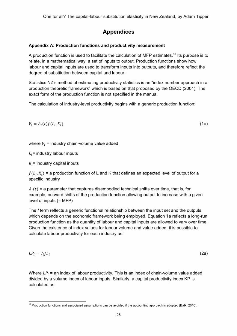
One for all? The capital-labour substitution elasticity in New Zealand, by Adam Tipper
28
Appendices
Appendix A: Production functions and productivity measurement
A production function is used to facilitate the calculation of MFP estimates.12 Its purpose is to
relate, in a mathematical way, a set of inputs to output. Production functions show how
labour and capital inputs are used to transform inputs into outputs, and therefore reflect the
degree of substitution between capital and labour.
Statistics NZ’s method of estimating productivity statistics is an “index number approach in a
production theoretic framework” which is based on that proposed by the OECD (2001). The
exact form of the production function is not specified in the manual.
The calculation of industry-level productivity begins with a generic production function:
�� � �����C���, �� (1a)
where �� = industry chain-volume value added ��= industry labour inputs �= industry capital inputs C���, �� = a production function of L and K that defines an expected level of output for a specific industry
����� = a parameter that captures disembodied technical shifts over time, that is, for example, outward shifts of the production function allowing output to increase with a given
level of inputs (= MFP)
The f term reflects a generic functional relationship between the input set and the outputs,
which depends on the economic framework being employed. Equation 1a reflects a long-run
production function as the quantity of labour and capital inputs are allowed to vary over time.
Given the existence of index values for labour volume and value added, it is possible to
calculate labour productivity for each industry as:
�4� � ��/�� (2a)
Where �4� = an index of labour productivity. This is an index of chain-volume value added divided by a volume index of labour inputs. Similarly, a capital productivity index KP is
calculated as:
12 Production functions and associated assumptions can be avoided if the accounting approach is adopted (Balk, 2010).
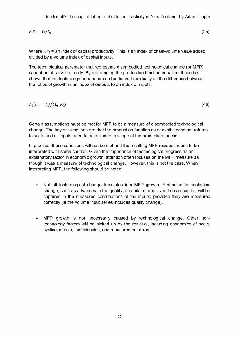
One for all? The capital-labour substitution elasticity in New Zealand, by Adam Tipper
29
4� � ��/ � (3a)
Where 4� = an index of capital productivity. This is an index of chain-volume value added divided by a volume index of capital inputs.
The technological parameter that represents disembodied technological change (or MFP)
cannot be observed directly. By rearranging the production function equation, it can be
shown that the technology parameter can be derived residually as the difference between
the ratios of growth in an index of outputs to an index of inputs:
����� � ��/C���, �� (4a)
Certain assumptions must be met for MFP to be a measure of disembodied technological
change. The key assumptions are that the production function must exhibit constant returns
to scale and all inputs need to be included in scope of the production function.
In practice, these conditions will not be met and the resulting MFP residual needs to be
interpreted with some caution. Given the importance of technological progress as an
explanatory factor in economic growth, attention often focuses on the MFP measure as
though it was a measure of technological change. However, this is not the case. When
interpreting MFP, the following should be noted:
• Not all technological change translates into MFP growth. Embodied technological
change, such as advances in the quality of capital or improved human capital, will be
captured in the measured contributions of the inputs; provided they are measured
correctly (ie the volume input series includes quality change).
• MFP growth is not necessarily caused by technological change. Other non-
technology factors will be picked up by the residual, including economies of scale,
cyclical effects, inefficiencies, and measurement errors.

One for all? The capital-labour substitution elasticity in New Zealand, by Adam Tipper
30
Appendix B: Industry coverage
Productivity industry coverage(1)
Measured sector industries Omitted industries
AA Agriculture LB Ownership of owner-occupied dwellings
AB Forestry and fishing MA Government administration and defence
BA Mining NA Education
CA Food, beverage, and tobacco manufacturing OA Health and community services
CB Textile and apparel manufacturing
CC Wood and paper products manufacturing
CD Printing, publishing, and recorded media
CE Petroleum, chemical, plastic, and rubber products manufacturing
CF Non-metallic mineral products manufacturing
CG Metal products manufacturing
CH Machinery and equipment manufacturing
CI Furniture and other manufacturing
DA Electricity, gas, and water supply
EA Construction
FA Wholesale trade
GA Retail trade
HA Accommodation, cafes, and restaurants
IA Transport and storage
JA Communication services
KA Finance and insurance
LA Property services(2)(3)
LC Business services(2)(3)
PA Cultural and recreational services(3)
QA Personal and other community services(2)(3)
1. Based on the Australian and New Zealand Standard Industrial Classification 1996 (ANZSIC96).
2. Included from March 1996 onwards in the measured sector. 3. Not included in this study.
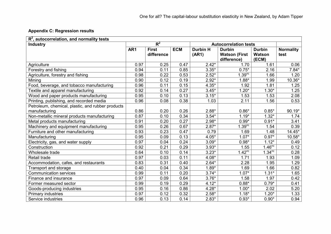
One for all? The capital-labour substitution elasticity in New Zealand, by Adam Tipper
Appendix C: Regression results
R2, autocorrelation, and normality tests
Industry R2 Autocorrelation tests
AR1 First difference
ECM Durbin H (AR1)
Durbin Watson (First difference)
Durbin Watson (ECM)
Normality test
Agriculture 0.97 0.25 0.47 2.42* 1.70 1.61 0.06
Forestry and fishing 0.94 0.11 0.85 3.35* 0.75* 2.16 7.84*
Agriculture, forestry and fishing 0.98 0.22 0.53 2.52* 1.39nc 1.66 1.20
Mining 0.90 0.12 0.19 2.92* 1.88* 1.99 10.36*
Food, beverage, and tobacco manufacturing 0.96 0.11 0.15 4.35* 1.92 1.81 1.25
Textile and apparel manufacturing 0.92 0.14 0.27 3.45* 1.20* 1.30* 1.25
Wood and paper products manufacturing 0.95 0.10 0.13 3.15* 1.53 1.53 2.08
Printing, publishing, and recorded media 0.96 0.08 0.38 1.03 2.11 1.56 0.53
Petroleum, chemical, plastic, and rubber products manufacturing 0.86 0.20 0.26 2.88* 0.86* 0.85* 90.19*
Non-metallic mineral products manufacturing 0.87 0.10 0.34 3.54* 1.19* 1.32* 1.74
Metal products manufacturing 0.91 0.20 0.27 2.98* 0.99* 0.91* 3.41
Machinery and equipment manufacturing 0.95 0.26 0.67 2.87* 1.39nc 1.54 0.39
Furniture and other manufacturing 0.93 0.23 0.47 0.79 1.69 1.48 14.45*
Manufacturing 0.95 0.09 0.13 4.05* 1.07* 0.97* 10.58*
Electricity, gas, and water supply 0.97 0.04 0.24 3.09* 0.98* 1.12* 0.49
Construction 0.92 0.21 0.29 3.93* 1.55 1.46nc 0.12
Wholesale trade 0.64 0.10 0.14 3.23* 1.42nc 1.34nc 0.28
Retail trade 0.97 0.03 0.11 4.08* 1.71 1.93 1.09
Accommodation, cafes, and restaurants 0.83 0.31 0.40 2.64* 2.28 1.95 1.29
Transport and storage 0.40 0.04 0.34 1.89* 1.69 1.66 0.82
Communication services 0.99 0.11 0.20 3.74* 1.07* 1.31* 1.65
Finance and insurance 0.97 0.09 0.64 3.76* 1.58 1.97 0.42
Former measured sector 0.99 0.19 0.29 4.12* 0.88* 0.79* 0.41
Goods-producing industries 0.95 0.16 0.86 4.28* 1.00* 2.02 5.20
Primary industries 0.97 0.12 0.32 2.58* 1.18* 1.20* 1.33
Service industries 0.96 0.13 0.14 2.83* 0.93* 0.90* 0.94
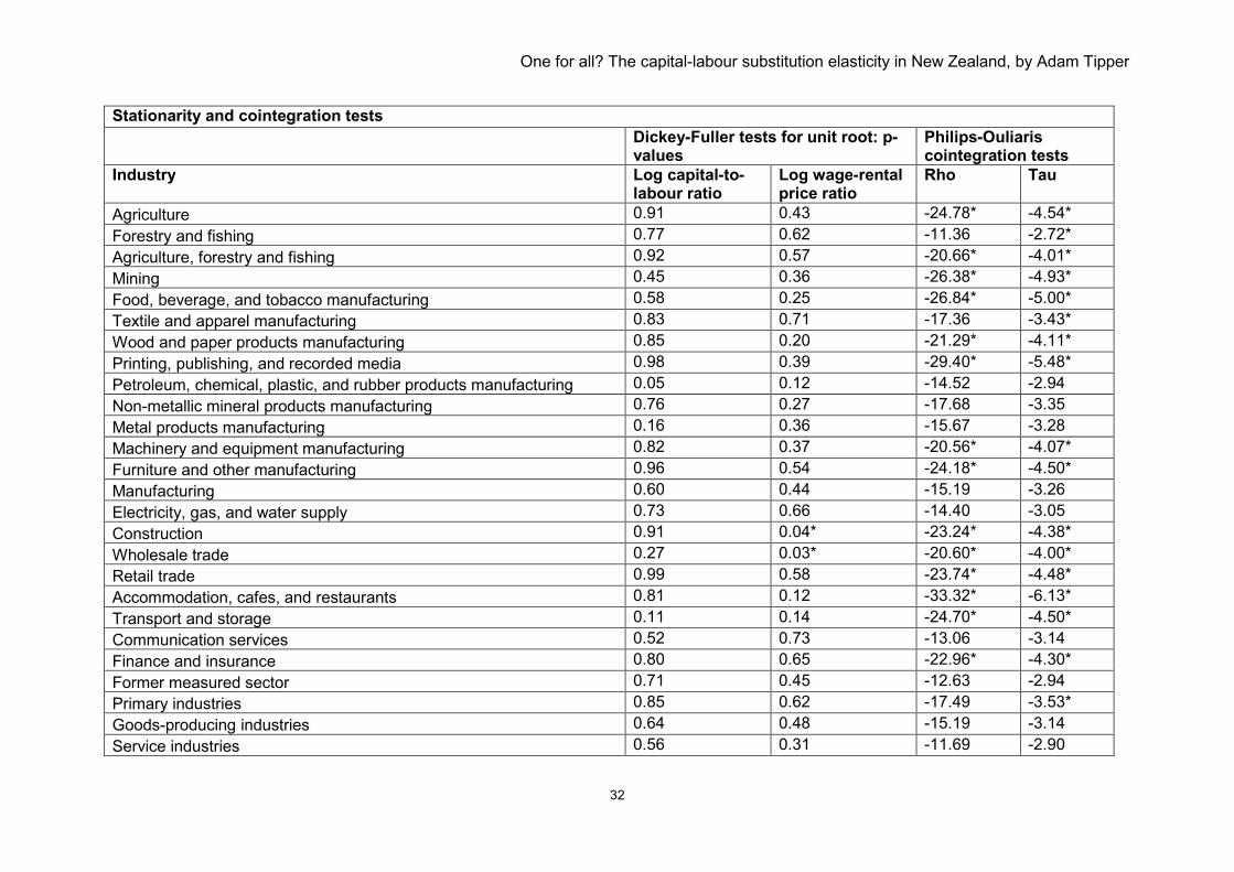
One for all? The capital-labour substitution elasticity in New Zealand, by Adam Tipper
32
Stationarity and cointegration tests
Dickey-Fuller tests for unit root: p-values
Philips-Ouliaris cointegration tests
Industry Log capital-to-labour ratio
Log wage-rental price ratio
Rho Tau
Agriculture 0.91 0.43 -24.78* -4.54*
Forestry and fishing 0.77 0.62 -11.36 -2.72*
Agriculture, forestry and fishing 0.92 0.57 -20.66* -4.01*
Mining 0.45 0.36 -26.38* -4.93*
Food, beverage, and tobacco manufacturing 0.58 0.25 -26.84* -5.00*
Textile and apparel manufacturing 0.83 0.71 -17.36 -3.43*
Wood and paper products manufacturing 0.85 0.20 -21.29* -4.11*
Printing, publishing, and recorded media 0.98 0.39 -29.40* -5.48*
Petroleum, chemical, plastic, and rubber products manufacturing 0.05 0.12 -14.52 -2.94
Non-metallic mineral products manufacturing 0.76 0.27 -17.68 -3.35
Metal products manufacturing 0.16 0.36 -15.67 -3.28
Machinery and equipment manufacturing 0.82 0.37 -20.56* -4.07*
Furniture and other manufacturing 0.96 0.54 -24.18* -4.50*
Manufacturing 0.60 0.44 -15.19 -3.26
Electricity, gas, and water supply 0.73 0.66 -14.40 -3.05
Construction 0.91 0.04* -23.24* -4.38*
Wholesale trade 0.27 0.03* -20.60* -4.00*
Retail trade 0.99 0.58 -23.74* -4.48*
Accommodation, cafes, and restaurants 0.81 0.12 -33.32* -6.13*
Transport and storage 0.11 0.14 -24.70* -4.50*
Communication services 0.52 0.73 -13.06 -3.14
Finance and insurance 0.80 0.65 -22.96* -4.30*
Former measured sector 0.71 0.45 -12.63 -2.94
Primary industries 0.85 0.62 -17.49 -3.53*
Goods-producing industries 0.64 0.48 -15.19 -3.14
Service industries 0.56 0.31 -11.69 -2.90

One for all? The capital-labour substitution elasticity in New Zealand, by Adam Tipper
33
Notes on the R2, autocorrelation, and normality tests table: For the autocorrelation tests, * indicates evidence for autocorrelation at the 95 percent level of significance, and nc denotes that the test is inconclusive. For the Jarque-Bera normality tests, * denotes significance at the 95 percent confidence level. Notes on the stationarity and cointegration test table: For the unit root tests, * denotes that the series does not contain a unit root. Test statistics for the Philips-Ouliaris cointegration tests are derived from the first difference model. Critical values from tables Ib and IIb from Philips-Ouliaris (1990) are: -20.4935 (rho) and -3.3654 (tau).* denotes that the test statistic is less than the critical value, and therefore provides evidence for cointegration.
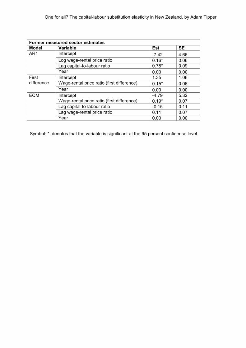
One for all? The capital-labour substitution elasticity in New Zealand, by Adam Tipper
Former measured sector estimates
Model Variable Est SE
AR1 Intercept -7.42 4.66
Log wage-rental price ratio 0.16* 0.06
Lag capital-to-labour ratio 0.78* 0.09
Year 0.00 0.00
First difference
Intercept 1.35 1.06
Wage-rental price ratio (first difference) 0.15* 0.06
Year 0.00 0.00
ECM
Intercept -4.79 5.32
Wage-rental price ratio (first difference) 0.19* 0.07
Lag capital-to-labour ratio -0.15 0.11
Lag wage-rental price ratio 0.11 0.07
Year 0.00 0.00
Symbol: * denotes that the variable is significant at the 95 percent confidence level.
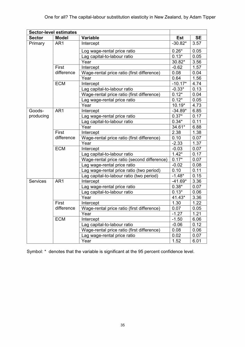
One for all? The capital-labour substitution elasticity in New Zealand, by Adam Tipper
35
Sector-level estimates Sector Model Variable Est SE
Primary AR1
Intercept -30.82* 3.57
Log wage-rental price ratio 0.26* 0.05
Lag capital-to-labour ratio 0.13* 0.05
Year 30.82* 3.56
First difference
Intercept -0.62 1.57
Wage-rental price ratio (first difference) 0.08 0.04
Year 0.64 1.56
ECM
Intercept -10.17* 4.74
Lag capital-to-labour ratio -0.33* 0.13
Wage-rental price ratio (first difference) 0.12* 0.04
Lag wage-rental price ratio 0.12* 0.05
Year 10.19* 4.73
Goods-producing
AR1
Intercept -34.89* 6.85
Lag wage-rental price ratio 0.37* 0.17
Lag capital-to-labour ratio 0.34* 0.11
Year 34.61* 6.88
First difference
Intercept 2.38 1.38
Wage-rental price ratio (first difference) 0.10 0.07
Year -2.33 1.37
ECM
Intercept -0.03 0.07
Lag capital-to-labour ratio 1.42* 0.17
Wage-rental price ratio (second difference) 0.17* 0.07
Lag wage-rental price ratio -0.02 0.08
Lag wage-rental price ratio (two period) 0.10 0.11
Lag capital-to-labour ratio (two period) -1.48* 0.15
Services AR1
Intercept -41.69* 3.36
Lag wage-rental price ratio 0.38* 0.07
Lag capital-to-labour ratio 0.13* 0.06
Year 41.43* 3.36
First difference
Intercept 1.30 1.22
Wage-rental price ratio (first difference) 0.07 0.05
Year -1.27 1.21
ECM
Intercept -1.50 6.06
Lag capital-to-labour ratio -0.06 0.12
Wage-rental price ratio (first difference) 0.08 0.06
Lag wage-rental price ratio 0.02 0.07
Year 1.52 6.01
Symbol: * denotes that the variable is significant at the 95 percent confidence level.
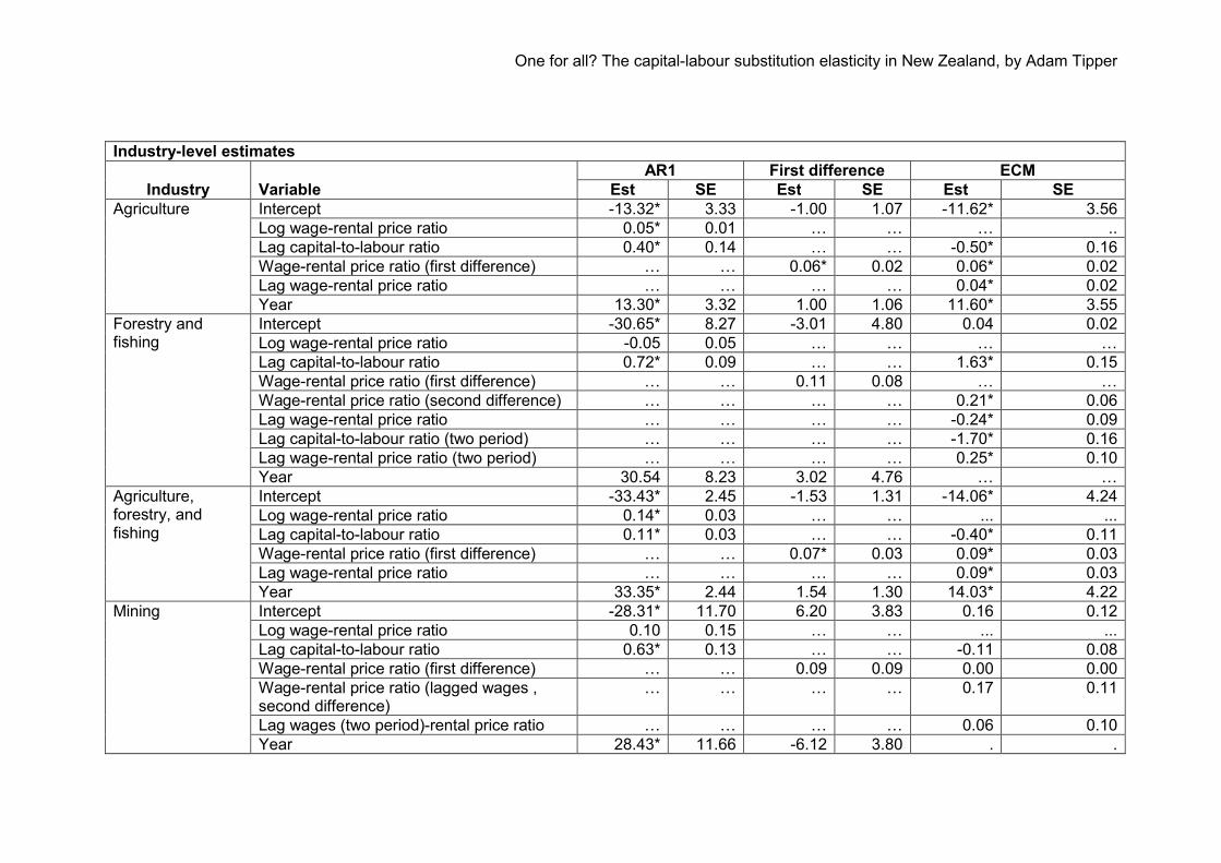
One for all? The capital-labour substitution elasticity in New Zealand, by Adam Tipper
Industry-level estimates
Industry Variable
AR1 First difference ECM
Est SE Est SE Est SE
Agriculture Intercept -13.32* 3.33 -1.00 1.07 -11.62* 3.56
Log wage-rental price ratio 0.05* 0.01 … … … ..
Lag capital-to-labour ratio 0.40* 0.14 … … -0.50* 0.16
Wage-rental price ratio (first difference) … … 0.06* 0.02 0.06* 0.02
Lag wage-rental price ratio … … … … 0.04* 0.02
Year 13.30* 3.32 1.00 1.06 11.60* 3.55
Forestry and fishing
Intercept -30.65* 8.27 -3.01 4.80 0.04 0.02
Log wage-rental price ratio -0.05 0.05 … … … …
Lag capital-to-labour ratio 0.72* 0.09 … … 1.63* 0.15
Wage-rental price ratio (first difference) … … 0.11 0.08 … …
Wage-rental price ratio (second difference) … … … … 0.21* 0.06
Lag wage-rental price ratio … … … … -0.24* 0.09
Lag capital-to-labour ratio (two period) … … … … -1.70* 0.16
Lag wage-rental price ratio (two period) … … … … 0.25* 0.10
Year 30.54 8.23 3.02 4.76 … …
Agriculture, forestry, and fishing
Intercept -33.43* 2.45 -1.53 1.31 -14.06* 4.24
Log wage-rental price ratio 0.14* 0.03 … … ... ...
Lag capital-to-labour ratio 0.11* 0.03 … … -0.40* 0.11
Wage-rental price ratio (first difference) … … 0.07* 0.03 0.09* 0.03
Lag wage-rental price ratio … … … … 0.09* 0.03
Year 33.35* 2.44 1.54 1.30 14.03* 4.22
Mining Intercept -28.31* 11.70 6.20 3.83 0.16 0.12
Log wage-rental price ratio 0.10 0.15 … … ... ...
Lag capital-to-labour ratio 0.63* 0.13 … … -0.11 0.08
Wage-rental price ratio (first difference) … … 0.09 0.09 0.00 0.00
Wage-rental price ratio (lagged wages , second difference)
… … … … 0.17 0.11
Lag wages (two period)-rental price ratio … … … … 0.06 0.10
Year 28.43* 11.66 -6.12 3.80 . .
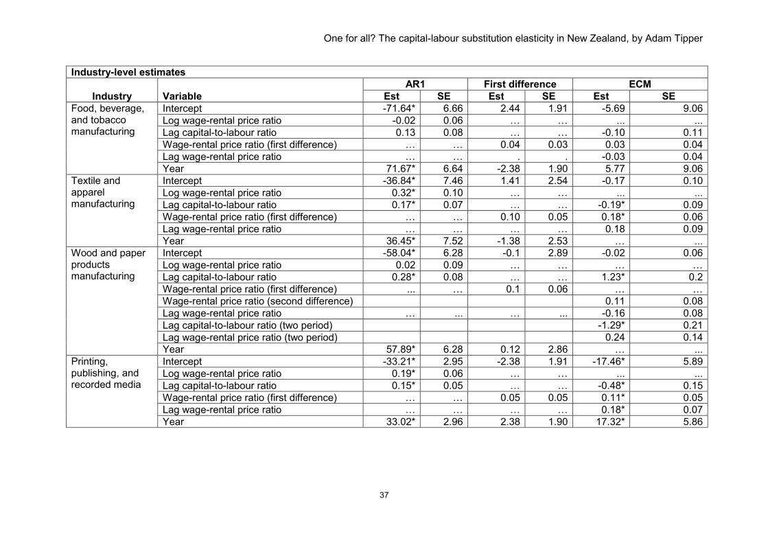
One for all? The capital-labour substitution elasticity in New Zealand, by Adam Tipper
37
Industry-level estimates
Industry Variable
AR1 First difference ECM
Est SE Est SE Est SE
Food, beverage, and tobacco manufacturing
Intercept -71.64* 6.66 2.44 1.91 -5.69 9.06
Log wage-rental price ratio -0.02 0.06 … … ... ...
Lag capital-to-labour ratio 0.13 0.08 … … -0.10 0.11
Wage-rental price ratio (first difference) … … 0.04 0.03 0.03 0.04
Lag wage-rental price ratio … … . . -0.03 0.04
Year 71.67* 6.64 -2.38 1.90 5.77 9.06
Textile and apparel manufacturing
Intercept -36.84* 7.46 1.41 2.54 -0.17 0.10
Log wage-rental price ratio 0.32* 0.10 … … ... ...
Lag capital-to-labour ratio 0.17* 0.07 … … -0.19* 0.09
Wage-rental price ratio (first difference) … … 0.10 0.05 0.18* 0.06
Lag wage-rental price ratio … … … … 0.18 0.09
Year 36.45* 7.52 -1.38 2.53 … ...
Wood and paper products manufacturing
Intercept -58.04* 6.28 -0.1 2.89 -0.02 0.06
Log wage-rental price ratio 0.02 0.09 … … … …
Lag capital-to-labour ratio 0.28* 0.08 … … 1.23* 0.2
Wage-rental price ratio (first difference) ... … 0.1 0.06 … …
Wage-rental price ratio (second difference) 0.11 0.08
Lag wage-rental price ratio … ... … ... -0.16 0.08
Lag capital-to-labour ratio (two period) -1.29* 0.21
Lag wage-rental price ratio (two period) 0.24 0.14
Year 57.89* 6.28 0.12 2.86 … ...
Printing, publishing, and recorded media
Intercept -33.21* 2.95 -2.38 1.91 -17.46* 5.89
Log wage-rental price ratio 0.19* 0.06 … … ... ...
Lag capital-to-labour ratio 0.15* 0.05 … … -0.48* 0.15
Wage-rental price ratio (first difference) … … 0.05 0.05 0.11* 0.05
Lag wage-rental price ratio … … … … 0.18* 0.07
Year 33.02* 2.96 2.38 1.90 17.32* 5.86
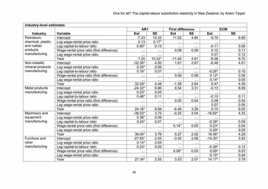
One for all? The capital-labour substitution elasticity in New Zealand, by Adam Tipper
38
Industry-level estimates
Industry Variable
AR1 First difference ECM
Est SE Est SE Est SE
Petroleum, chemical, plastic, and rubber products manufacturing
Intercept -7.23 10.32 11.52 4.84 6.70 6.69
Log wage-rental price ratio 0.13 0.17* … … ... ...
Lag capital-to-labour ratio 0.80* 0.13 … … -0.11 0.08
Wage-rental price ratio (first difference) … … 0.08 0.09 0.12 0.11
Lag wage-rental price ratio … … . . 0.07 0.12
Year 7.25 10.33* -11.40 4.81 -6.58 6.70
Non-metallic mineral products manufacturing
Intercept -32.36* 4.50 1.61 2.67 -6.48 4.61
Log wage-rental price ratio 0.30* 0.06 … … ... ...
Lag capital-to-labour ratio 0.16* 0.07 … … -0.26* 0.10
Wage-rental price ratio (first difference) … … 0.09 0.06 0.12* 0.06
Lag wage-rental price ratio … … … … 0.14* 0.05
Year 32.28* 4.48 -1.58 2.64 6.47 4.59
Metal products manufacturing
Intercept -24.32* 6.96 6.54 3.31 -0.13 6.09
Log wage-rental price ratio 0.23* 0.05 … … ... ...
Lag capital-to-labour ratio 0.46* 0.11 … … -0.15 0.11
Wage-rental price ratio (first difference) … … 0.05 0.04 0.08 0.04
Lag wage-rental price ratio … … … … 0.07 0.05
Year 24.16* 6.94 -6.46 3.28 0.15 6.05
Machinery and equipment manufacturing
Intercept -36.53* 3.75 -0.25 2.04 -16.82* 4.33
Log wage-rental price ratio 0.38* 0.06 … … ... ...
Lag capital-to-labour ratio 0.24* 0.07 … … -0.39* 0.09
Wage-rental price ratio (first difference) … … 0.14* 0.05 0.23* 0.04
Lag wage-rental price ratio … … … … 0.29* 0.05
Year 36.04* 3.76 0.27 2.02 16.46* 4.29
Furniture and other manufacturing
Intercept -27.65* 2.55 -3.55 2.08 -14.35* 3.83
Log wage-rental price ratio 0.14* 0.04 … … ... ...
Lag capital-to-labour ratio 0.23* 0.05 … … -0.39* 0.12
Wage-rental price ratio (first difference) … … 0.08* 0.03 0.09* 0.03
Lag wage-rental price ratio … … … … 0.10* 0.04
Year 27.34* 2.55 3.53 2.07 14.17* 3.79
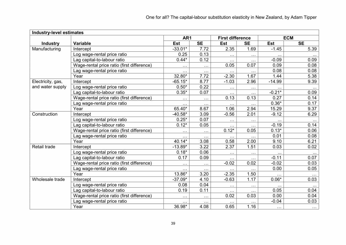
One for all? The capital-labour substitution elasticity in New Zealand, by Adam Tipper
39
Industry-level estimates
Industry Variable
AR1 First difference ECM
Est SE Est SE Est SE
Manufacturing Intercept -33.01* 7.72 2.35 1.69 -1.45 5.39
Log wage-rental price ratio 0.25 0.13 … … ... ...
Lag capital-to-labour ratio 0.44* 0.12 … … -0.09 0.09
Wage-rental price ratio (first difference) … … 0.05 0.07 0.09 0.08
Lag wage-rental price ratio … … … … 0.08 0.08
Year 32.80* 7.72 -2.30 1.67 1.44 5.38
Electricity, gas, and water supply
Intercept -65.15* 8.77 -1.03 2.96 -14.99 9.39
Log wage-rental price ratio 0.50* 0.22 … … ... ...
Lag capital-to-labour ratio 0.35* 0.07 … … -0.21* 0.09
Wage-rental price ratio (first difference) … … 0.13 0.13 0.27 0.14
Lag wage-rental price ratio … … … … 0.36* 0.17
Year 65.40* 8.67 1.06 2.94 15.29 9.37
Construction Intercept -40.58* 3.09 -0.56 2.01 -9.12 6.29
Log wage-rental price ratio 0.25* 0.07 … … ... ...
Lag capital-to-labour ratio 0.12* 0.05 … … -0.19 0.14
Wage-rental price ratio (first difference) … … 0.12* 0.05 0.13* 0.06
Lag wage-rental price ratio … … … … 0.01 0.08
Year 40.14* 3.08 0.58 2.00 9.10 6.21
Retail trade Intercept -13.89* 3.22 2.37 1.51 0.03 0.02
Log wage-rental price ratio 0.18* 0.06 … … ... ...
Lag capital-to-labour ratio 0.17 0.09 … … -0.11 0.07
Wage-rental price ratio (first difference) … … -0.02 0.02 -0.02 0.03
Lag wage-rental price ratio … … … … 0.00 0.05
Year 13.86* 3.20 -2.35 1.50 … …
Wholesale trade Intercept -37.09* 4.10 -0.63 1.17 0.06* 0.03
Log wage-rental price ratio 0.08 0.04 … … ... ...
Lag capital-to-labour ratio 0.19 0.11 … … 0.05 0.04
Wage-rental price ratio (first difference) … … 0.02 0.03 0.00 0.04
Lag wage-rental price ratio … … … … -0.04 0.03
Year 36.98* 4.08 0.65 1.16 … …
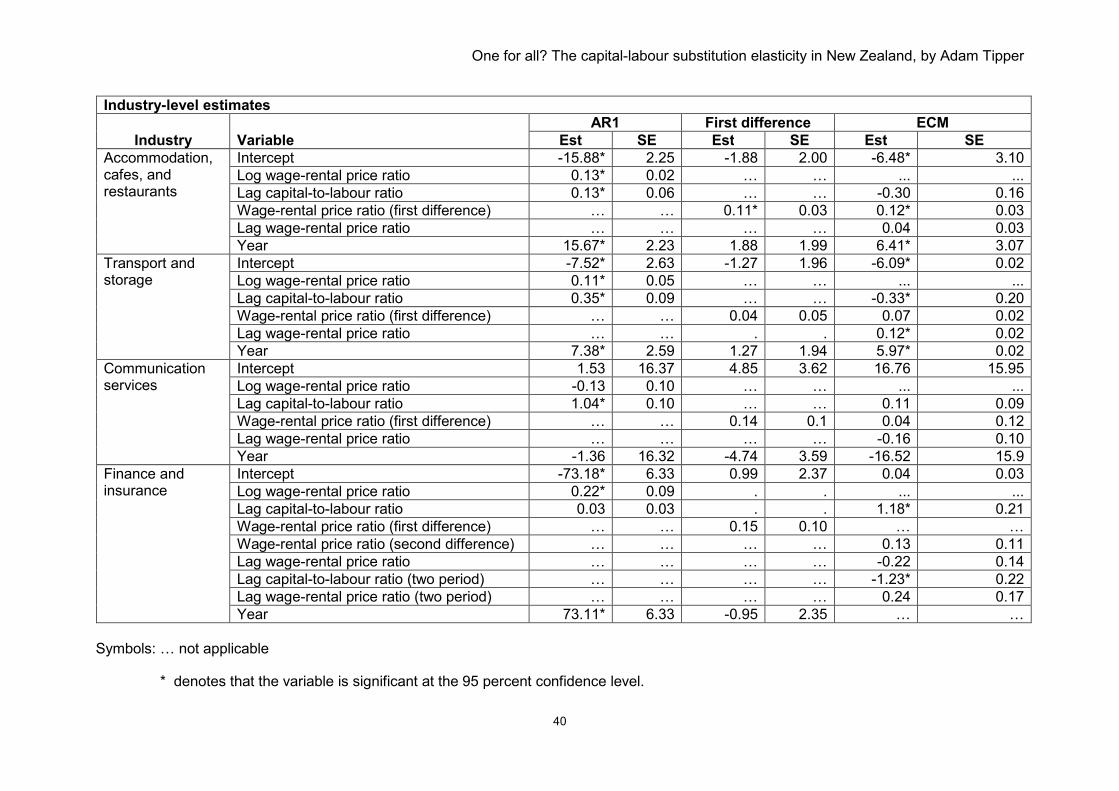
One for all? The capital-labour substitution elasticity in New Zealand, by Adam Tipper
40
Industry-level estimates
Industry Variable
AR1 First difference ECM
Est SE Est SE Est SE
Accommodation, cafes, and restaurants
Intercept -15.88* 2.25 -1.88 2.00 -6.48* 3.10
Log wage-rental price ratio 0.13* 0.02 … … ... ...
Lag capital-to-labour ratio 0.13* 0.06 … … -0.30 0.16
Wage-rental price ratio (first difference) … … 0.11* 0.03 0.12* 0.03
Lag wage-rental price ratio … … … … 0.04 0.03
Year 15.67* 2.23 1.88 1.99 6.41* 3.07
Transport and storage
Intercept -7.52* 2.63 -1.27 1.96 -6.09* 0.02
Log wage-rental price ratio 0.11* 0.05 … … ... ...
Lag capital-to-labour ratio 0.35* 0.09 … … -0.33* 0.20
Wage-rental price ratio (first difference) … … 0.04 0.05 0.07 0.02
Lag wage-rental price ratio … … . . 0.12* 0.02
Year 7.38* 2.59 1.27 1.94 5.97* 0.02
Communication services
Intercept 1.53 16.37 4.85 3.62 16.76 15.95
Log wage-rental price ratio -0.13 0.10 … … ... ...
Lag capital-to-labour ratio 1.04* 0.10 … … 0.11 0.09
Wage-rental price ratio (first difference) … … 0.14 0.1 0.04 0.12
Lag wage-rental price ratio … … … … -0.16 0.10
Year -1.36 16.32 -4.74 3.59 -16.52 15.9
Finance and insurance
Intercept -73.18* 6.33 0.99 2.37 0.04 0.03
Log wage-rental price ratio 0.22* 0.09 . . ... ...
Lag capital-to-labour ratio 0.03 0.03 . . 1.18* 0.21
Wage-rental price ratio (first difference) … … 0.15 0.10 … …
Wage-rental price ratio (second difference) … … … … 0.13 0.11
Lag wage-rental price ratio … … … … -0.22 0.14
Lag capital-to-labour ratio (two period) … … … … -1.23* 0.22
Lag wage-rental price ratio (two period) … … … … 0.24 0.17
Year 73.11* 6.33 -0.95 2.35 … …
Symbols: … not applicable
* denotes that the variable is significant at the 95 percent confidence level.