Noname manuscript No.(will be inserted by the editor)

One-dimensional turbulence modeling for cylindrical and sphericalflows: Model formulation and application

David O. Lignell · Victoria B. Lansinger · JuanMedina · Marten Klein · Alan R. Kerstein · HeikoSchmidt · Marco Fistler · Michael Oevermann

Received: date / Accepted: date

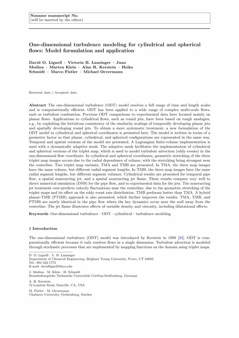
Abstract The one-dimensional turbulence (ODT) model resolves a full range of time and length scalesand is computationally efficient. ODT has been applied to a wide range of complex multi-scale flows,such as turbulent combustion. Previous ODT comparisons to experimental data have focused mainly onplanar flows. Applications to cylindrical flows, such as round jets, have been based on rough analogies,e.g., by exploiting the fortuitous consistency of the similarity scalings of temporally developing planar jetsand spatially developing round jets. To obtain a more systematic treatment, a new formulation of theODT model in cylindrical and spherical coordinates is presented here. The model is written in terms of ageometric factor so that planar, cylindrical, and spherical configurations are represented in the same way.Temporal and spatial versions of the model are presented. A Lagrangian finite-volume implementation isused with a dynamically adaptive mesh. The adaptive mesh facilitates the implementation of cylindricaland spherical versions of the triplet map, which is used to model turbulent advection (eddy events) in theone-dimensional flow coordinate. In cylindrical and spherical coordinates, geometric stretching of the threetriplet map images occurs due to the radial dependence of volume, with the stretching being strongest nearthe centerline. Two triplet map variants, TMA and TMB are presented. In TMA, the three map imageshave the same volume, but different radial segment lengths. In TMB, the three map images have the sameradial segment lengths, but different segment volumes. Cylindrical results are presented for temporal pipeflow, a spatial nonreacting jet, and a spatial nonreacting jet flame. These results compare very well todirect numerical simulation (DNS) for the pipe flow, and to experimental data for the jets. The nonreactingjet treatment over-predicts velocity fluctuations near the centerline, due to the geometric stretching of thetriplet maps and its effect on the eddy event rate distribution. TMB performs better than TMA. A hybridplanar-TMB (PTMB) approach is also presented, which further improves the results. TMA, TMB, andPTMB are nearly identical in the pipe flow where the key dynamics occur near the wall away from thecenterline. The jet flame illustrates effects of variable density and viscosity, including dilatational effects.

Keywords One-dimensional turbulence · ODT · cylindrical · turbulence modeling

1 Introduction

The one-dimensional turbulence (ODT) model was introduced by Kerstein in 1999 [23]. ODT is com-putationally efficient because it only resolves flows in a single dimension. Turbulent advection is modeledthrough stochastic processes that are implemented by mapping functions on the domain using triplet maps.

D. O. Lignell · V. B. LansingerDepartment of Chemical Engineering, Brigham Young University, Provo, UT 84602Tel.: 801-422-1772E-mail: davidlignell@byu.edu

J. Medina · M. Klein · H. SchmidtBrandenburgische Technische Universitat Cottbus-Senftenberg, Germany

A. R. Kerstein72 Lomitas Road, Danville, CA, USA

M. Fistler · M. OevermannChalmers University, Gothenburg, Sweden

In ODT, the terms “eddy event” and “eddies” are historically used to denote these stochastic mapping pro-cesses. Eddy events occur concurrently with the solution of unsteady one-dimensional transport equationsfor momentum and other scalar quantities. Eddy event locations, sizes, and occurrence rates are specifieddynamically and locally using the momentum fields that evolve with the flow. (Temperature fields or scalarfields are also used for buoyant flows.) Because the model is one-dimensional, it is limited to homogeneousor boundary layer flows, such as jets, wakes, mixing layers, and channel flows. These flows, however, areextremely common in turbulence research.

While ODT does not replace other turbulent simulation approaches, such as LES or DNS, the compu-tational efficiency of ODT, combined with its resolution of a full range of scales, make it a useful tool thatcomplemements traditional simulation tools. For example, LES resolves large-scale turbulent structures butmodels subgrid scale processes. Such modeling, e.g., for reacting flows, is often done in a chemical statespace [9]. In contrast, ODT resolves (in one dimension) fine scale diffusive and reactive structures in thenatural physical coordinate (like DNS) but models large-scale advection.

ODT has been applied by a number of researchers to a wide range of flows. Early applications focusedon configurations such as homogeneous turbulence, wakes, and mixing layers [23,25], and utilized onlya single velocity component. Wunsch and Kerstein [54] studied layer formation in stratified flow. Theyadded buoyant forcing effects to the shear forces normally used to specify ODT eddy rates. A kernelfunction K (with a coefficient c) was added to the triplet mapped velocity field to enable potential–kineticenergy exchange. Kerstein et al. [24] generalized this use of a kernel function and extended ODT to avector formulation in which three velocity components are transported, with energy transfers among thecomponents reflecting pressure-scrambling and return-to-isotropy phenomena. Ashurst and Kerstein [2]extended this approach to variable density flows, where an additional kernel J (with coefficient b) wasadded to triplet mapped velocity components to ensure conservation of both momentum and energy invariable density flows. These researchers also presented the formal “spatial” formulation of ODT in whichthe simulation is advanced in a downstream spatial coordinate rather than in time, as is done in the“temporal” ODT formulation. These advancements have facilitated ODT’s application to more complexflows, including combustion in jets [10,15,16,43,34,32,21] and fires [17,18,49,45,39], particle flows [46,52,14,51], and subgrid modeling for LES [5,48,47].

All of these simulated flows (and others not cited) used the planar formulation of ODT, even whencomparing to experiments of cylindrical configurations. This comparison is reasonable for round jets becausethe Reynolds number is axially invariant in both constant-property spatial round jets and constant-propertytemporal planar jets [51]. To compare temporal ODT simulations to spatial experimental simulations,however, time on the ODT line must be converted to experimental axial spatial locations. This is normallydone using a mean line velocity (such as the ratio of the integrated momentum flux to the integrated massflux) [51], but this implies that all fluid parcels on the line have the same axial location time history. Thisassumption is not ideal for phenomena that are sensitive to time history, such as soot formation, flameextinction and reignition processes, and particle-turbulence interactions.

These limitations in applying the planar ODT formulation to cylindrical flows motivate the work pre-sented here. In this paper, we extend the ODT model from the planar formulation to cylindrical andspherical formulations. There have been some previous efforts to implement cylindrical and spherical ODTformulations. Krishnamoorthy [27] implemented a cylindrical ODT formulation and applied the model inpipe and jet configurations. Lackmann et al. [28] implemented a spherical formulation of the linear eddymodel (LEM) for engine applications. Here, we give a detailed description of cylindrical and spherical for-mulations of ODT. While the spherical formulation is included for completeness, we focus on the cylindricalformulation because it is most directly applicable to current and previous ODT research efforts. We deferto the literature for much of the existing ODT model formulation, e.g., [2,24,33], and focus on the newcylindrical and spherical geometries. For completeness, however, we include a summary of the ODT modelformulation. We present results for the cylindrical formulation applied to a pipe flow, a round nonreactingspatial jet, and a round jet flame. A more detailed study of pipe flow than is possible in this paper is pre-sented by Medina et al. [36]. Nevertheless, pipe flow is revisited in the present study because it is a usefulcase for exhibiting the effects of some of the refinements of the cylindrical formulation that are introducedhere.

2 Cylindrical and spherical ODT formulations

Since we are emphasizing the model for cylindrical flows in this paper, we will only refer to the cylindri-cal formulation, while the spherical formulation is implied. Physically important spherical flows occur in

2

y

y

z

x

x

xq

F

Ax

Ax

Ax

Ay

Ay

LyLx

Ly

Fig. 1 Schematic diagram of cell volumes for planar (top), cylindrical (middle), and spherical (bottom) formulations.

geophysical and astrophysical fluid dynamics, including flows in planets and stars, e.g., spherical Rayleigh-Benard convection [12].

The new formulation affects the two primary aspects of the ODT model: (i) the specification of the eddyevents through triplet maps and (ii) the one-dimensional evolution equations for transported quantities.Since ODT models turbulent advection solely through the eddy events, the evolution of the transportequations amounts to the solution of unsteady, one-dimensional partial differential equations that includediffusive and source terms. The sequencing of these operations during ODT advancement is described inAppendix A.

In the following, we will take x to be the line-oriented direction, while y and z are off-line directions.For planar and cylindrical geometries, y is taken to be the streamwise and axial directions, respectively.For cylindrical and spherical geometries, we will take x to be negative left of the origin and positive rightof the origin.

We present the ODT model in terms of a discrete finite-volume formulation with grid cells (controlvolumes) defined by their face locations and cell positions located midway between the faces. For consistencywith [33], we will refer to the left and right cell face locations as west and east, with subscripts e and w,respectively. Considering discrete grid cells also facilitates the description of the eddy events in the nextsection. Fig. 1 shows schematic diagrams of control volumes for the three geometries considered. Ax andAy are the face areas perpendicular to the x and y directions, respectively; lengths Lx and Ly are alsoshown. In cylindrical and spherical configurations, the domain is interpreted as double wedges or doublecones of arbitrary angle θ or solid angle Φ, respectively. Note that x and r are synonymous. (In the sphericalcase shown in the figure, the radial coordinate is shown, but the two angular coordinates are not explicitlyshown.) For positive cell faces located at xf,e and xf,w, the cell volumes for planar, cylindrical, and spherical

configurations are Vp =LyLz

1 (xf,e−xf,w), Vc =Lyθ2 (x2f,e−x2f,w), and Vs = Φ

3 (x3f,e−x3f,w). When definingvolumes on the one-dimensional domain, we can use arbitrary cell side lengths Ly and Lz in the y and zdirections, as well as arbitrary angle θ and solid angle Φ. These quantities are ultimately normalized out ofthe formulation and results since ODT outputs and time advanced properties are intensive quantities. Ingeneral, we have

V =

1c (xcf,e − xcf,w) if xf,w ≥ 0,1c (|xf,w|c − |xf,e|c) if xf,e ≤ 0,1c (|xf,w|c + xcf,e) if xf,w < 0 < xf,e,

(1)

where c is 1, 2, or 3, for planar, cylindrical, and spherical, respectively. For the second case in Eq. 1, fornegative xf,e, the positions of xf,e and xf,w are reversed due to symmetry about the origin. The third casecorresponds to a cell that contains the origin, in which case the volume is the sum of the wedge (or cone)volumes on either side of the origin.

In planar and cylindrical geometries, the areas Ay in Fig. 1 are their respective volumes divided by Ly.For a positive face position xf , the face areas Ax are given by LyLz, Lyθxf = Lyθr, and Φx2f = Φr2 for

3

0

xbefore triplet map:

after triplet map:

b1 g1a1 b2 a2g2 b3 g3a3

0

bo goao

Fig. 2 Schematic diagram of a cylindrical triplet map. The map region is shaded. There are three grid cells before thetriplet map, and nine cells after. After the triplet map, the three map images are separately shaded; each image of a givenpre-map cell has the same volume (one-third the original volume). The nine final cells are labeled by the cells from whichthey originate.

planar, cylindrical, and spherical, respectively. In general, for arbitrary Ly, Lz, θ, and Φ, we take

Ax = |xf |c−1. (2)

2.1 Eddy events

2.1.1 Triplet map A (TMA)

In the planar formulation of ODT, turbulent advection is modeled using stochastic, instantaneous eddyevents. Within an eddy event, advection is implemented using the so-called triplet map [22]. (Other oper-ations performed during an eddy event are discussed in Sec. 2.2.)

The triplet map is defined as follows. A region of the domain is selected such that x0 ≤ x ≤ x0 + l,where x0 is the location of the left edge of the eddy and l is the eddy size. For a given scalar profile inthe eddy region (such as a momentum component), three images of the profile are made. Each profile iscompressed spatially by a factor of three and lined up along the domain in the eddy region. The middlecopy is then spatially inverted (mirrored). This is applied to all transported properties. The triplet mapis strictly conservative of all quantities and their statistical moments, and property profiles (though notproperty gradients) remain continuous. The triplet map increases scalar gradients and decreases lengthscales consistent with the effects of turbulent eddies in real flows. The maps are also local in the sense thatscales decrease by a factor of three. Subsequent eddies in the same region will further decrease the scalesby this factor, resulting in a cascade of scales. Eddy rates depend on the eddy size and the local kineticenergy field such that the eddy events follow turbulent cascade scaling laws.

For cylindrical and spherical flows, the triplet map formulation is modified. This can be done in severalways. In the first approach, here denoted TMA, we proceed similarly to the planar case, but rather thansplit the eddy region into thirds by distance, we split the eddy region into thirds by volume. These areequivalent for the planar case, but not in the cylindrical or spherical cases.

Fig. 2 is a schematic of a cylindrical eddy in the right half of the domain. The triplet-map region initiallycontains three cells labeled α0, β0, and γ0. The post-triplet-map state has three images of the original profile(three copies of the original three cells), and each image (and each cell within) has one-third of its originalvolume. Note the spatial inversion of the middle image.

The triplet map is implemented by specifying its effects on the cell locations and the cell contents.Before the map, the volume of each cell is recorded. The number of cells in the eddy region is tripled duringthe map, facilitated by an adaptive grid [33]. The locations of the edges of the eddy are unchanged by themap. The new interior cell face positions can then be computed sequentially from one edge of the eddy tothe other. For example, we can march eastward from the west edge using the solution of Eq. (1) for thelocation xf,e of the east face of each successive cell, namely

xf,e =

(xcf,w + cFV V

)1/cif xf,w ≥ 0,

− (|xf,w|c − cFV V )1/c if xf,e ≤ 0,

(−|xf,w|c + cFV V )1/c if xf,w < 0 < xf,e.

(3)

4

0position x

TMB

TMA

prop

erty

Fig. 3 Illustration of the effects of versions TMA and TMB of the cylindrical triplet map on the originally linear profileconnecting the ends of each curve. Thick curves are mapped property profiles. Vertical dashed lines mark the radial 1/3and 2/3 positions of the maps.

Here, FV is a fractional multiplier of the volume under the triplet map (FV = 1/3 for TMA). Note that,while shown in Fig. 2 for simplicity, the initial radial (x) intervals of cells α0, β0, and γ0 do not need tobe equal. Also, the edges of the triplet map do not normally coincide with cell faces; in that case, only theportion of a cell contained within the triplet map region is modified by the map. In Fig. 2, the interior cellsα and γ after the triplet map would have one-third the volume of the portion of the respective original cellthat was within the map region.

Some additional algebraic complexity arises if an eddy edge or a boundary between post-map imagesis contained within the interior of a cell. Indeed, these locations do not typically coincide with cell faces.Conceptually, this is handled by assuming the insertion of virtual cell faces at the eddy edges and imageboundaries, which reduces these cases to the treatment that has been described.

Relative to the planar case, the cylindrical triplet map tends to stretch profiles nearer to the origin andcompress profiles farther from the origin since the volume per unit radial distance is larger at higher radialdistance (see Fig. 3 below).

2.1.2 Triplet map B (TMB)

An alternative triplet map, denoted TMB, is also considered. Rather than define the three images on anequal volume basis, the three images are defined on an equal radial interval basis. The volume fraction ofeach image is then computed using the volume-position relations in Eq. (1), where the positions xf are theeddy edges, or the 1/3 or 2/3 image boundaries, and the image volume fractions FV are then outputs ratherthan inputs. Using TMA, the volume fractions of the three images were each 1/3. TMB is implementedin much the same way as TMA, but the cell volume V in Eq. (3) is multiplied by the appropriate volumefraction FV for the given image that the cell is mapped to rather than 1/3. Conservation is maintainedsince the volume fractions of the three images in TMB sum to unity.

A schematic of the action of TMA is shown in Fig. 2, where, for the β cells (for example), Vβ1= Vβ2

=Vβ3

= Vβ0/3. For both TMA- and TMB-type triplet maps we have Vβ1

+ Vβ2+ Vβ3

= Vβ0. However, for

a TMB-type map, Vβ1volume in Fig. 2 would be smaller than Vβ2

, and Vβ3because the left image would

have a smaller outer radius.

Figure 3 illustrates the effect of TMA and TMB on initially linear profiles in a cylindrical configuration.Three maps TMA and TMB are shown at three radial locations. The vertical dashed lines are guidelinesindicating the interior 1/3 and 2/3 positions of the maps. Note that these positions coincide with the highand low peaks for TMB, but not for TMA. Compare the left and right image of the middle TMA and TMBmaps in Fig. 3. The left image of TMB is narrower (radially) than in TMA, and the right image of TMBis wider (radially) than in TMA; the resulting cell volumes in the left image of TMB are smaller than inTMA, and cell volumes in the right image of TMB are larger than in TMA. The stretching of TMA inreference to the location of the peaks relative to the 1/3 and 2/3 positions becomes less significant withincreasing distance from the origin.

5

0position x

prop

erty

TMATMB

Fig. 4 TMA and TMB for maps centered on the origin for initially linear property profiles.

Both TMA and TMB exhibit nonlinear profiles within each of the three map images in Fig. 3. In thisdiscussion, the nonlinearity occurs in relation to the initially linear profiles, which are used to illustrate asimple case. In general, the initial profile will be arbitrary. For planar flows, the three images are linearlycompressed images of the initial profile; TMA and TMB result in identical mappings. In cylindrical andspherical flows, the three images exhibit some geometric distortion, as exhibited in Fig. 3. TMB reducesthe geometric stretching compared to TMA in the sense that the three map images in Fig. 3 each havethe same one-third radial segment lengths. The profiles within the segments are still stretched relative to aplanar triplet map (whose image profiles would be linear in Fig. 3) and this is most notable near the originat x = 0.

Figure 4 shows triplet maps centered on the origin for initially linear profiles for TMA and TMB. Asexpected, these maps are symmetric. Interestingly, the center image in each map preserves the linearity ofthe initial profile. This linearity is a consequence of the symmetry about the origin. In the center image,the (positive x or negative x) volume enclosed at any position is computed from Eq. (1) with xf,i = 0.For example, for positive x, if a pre-map position is xpre, the volume is Vpre = 1

c (xcpre − 0). The post-map

volume is FV Vpre, and the post-map position from Eq. (3) is xpost = (0 + cFV Vpre)1/c = F

1/cV xpre, where

FV was defined above as the fraction applied to the volume for the given image (Fv = 1/3 for TMA).Hence, the post-map positions in the center image are proportional to the pre-map positions, resulting ina linear profile.

The center image through the origin in Fig. 4 is linear with nonzero slope as discussed above. This isin contrast to the post-map image through the origin shown in Fig. 3, where the profile at the origin haszero slope. This zero slope is due to the infinite compression there, which does not happen for the specialcase of Fig. 4. This flattening at x = 0 in Fig. 3 is a signature of the so-called “geometric lensing” effect,which is discussed further below.

2.2 Eddy selection and implementation

2.2.1 Eddy implementation

As explained in Sec. 2.1, advection is implemented within an eddy event using the triplet map. Additionally,ODT velocity component profiles are modified during the eddy event. This reflects the difference betweenflow evolution and scalar evolution. A conserved passive scalar, for example, is subject only to advectionand diffusion. In ODT, molecular diffusion is advanced in time during the time intervals between eddyoccurrences, as elaborated in Sec. 2.3 and Appendix A. Therefore, during an eddy event, conserved passivescalars and, more generally, properties other than velocity components, are subject only to the triplet map,but velocity profiles, as well as being triplet mapped, are subject to an additional modification. This reflectsthe fact that moment advancement involves pressure–gradient forcing (and possibly other body forcing) aswell as advection and viscous transport, the latter of which is subsumed in the abovementioned treatmentof molecular diffusion.

6

Unlike advection, which displaces fluid without changing its internal state, body forcing changes thefluid’s internal state. This change can include quantities other than velocity; such effects are minor andtherefore omitted for flow regimes considered here but included in a previous ODT formulation [20]. How-ever, velocity profiles require modification during eddy events in order to enforce momentum and energyconservation in all situations and capture additional relevant phenomenology.

On this basis, the velocity change during an eddy event is symbolically denoted

ui(x)→ u′i(x) + ciK(x) + biJ(x). (4)

Here and in the remainder of the model description, it is convenient to denote velocity components usingsubscripts. Pre-triplet map velocity components are denoted as ui(x), while u′i(x) and other primed quan-tities below refer to post-triplet map quantities. K(x) and J(x) are kernel functions, akin to wavelets, thatare not uniquely prescribed by conservation laws. It is convenient to define K(x) as the displacement of apoint from its initial position by a triplet map and to let J(x) = |K(x)|. ci and bi are coefficients set bythe constraint that momentum and energy are conserved, incorporating external sources and sinks whereapplicable.

For planar geometry, the definition of K(x) specializes to [2,24]

K(x) = x− x0 −

3(x− x0) if x0 ≤ x ≤ x0 + 1

3 l,

2l − 3(x− x0) if x0 + 13 l ≤ x ≤ x0 + 2

3 l,

3(x− x0)− 2l if x0 + 23 l ≤ x ≤ x0 + l,

x− x0 otherwise.

(5)

In practice, K(x) is evaluated from map-induced displacements of cell centers so that a single numericalprocedure holds for all geometries (planar, cylindrical, and spherical) and both triplet map types (TMAand TMB).

Let Qi denote the available eddy-integrated kinetic energy of component i; in other words, Qi is themaximum energy extractable by adding arbitrary multiples of the K and J kernels to the triplet-mappedcomponent i velocity profile, subject to momentum conservation. The total available kinetic energy,

Ekin =∑i

Qi, (6)

is a key input to the eddy selection process described in Sec. 2.2.2. Ekin is a natural basis for eddy selectionbecause any coupling of the eddy to an external energy sink that exceeds Ekin should be energeticallyforbidden, thereby preventing eddy implementation.

Momentum conservation allows bi in Eq. (4) to be expressed in terms of ci and given quantities. Toevaluate Qi, the eddy-integrated kinetic energy is evaluated for ci = bi = 0 and for the value of ci thatminimizes the eddy-integrated kinetic energy. By definition, Qi is the former minus the latter. Following[2], but using a more general notation applicable to the three coordinate systems used here, this gives

Qi =P 2i

4S, (7)

7

where

Pi = ui,ρK −Aui,ρJ , (8)

S =1

2(A2 + 1)ρKK −AρKJ , (9)

A =ρKρJ

, (10)

ρK =

∫V

ρ′K dV, (11)

ρJ =

∫V

ρ′J dV, (12)

ρKK =

∫V

ρ′K2 dV, (13)

ρKJ =

∫V

ρ′KJ dV, (14)

ui,ρK =

∫V

u′iρ′K dV, (15)

ui,ρJ =

∫V

u′iρ′J dV. (16)

All quantities in the integrands above depend only on x, and the indicated volume integration subsumesthe x dependence of volume increments, as implied by specialization of Fig. 1 to infinitesimal x increments.The integrals are numerically implemented as sums over the grid cells in the eddy region, with dV replacedby cell volumes, evaluated using Eq. (1). The planar expressions in [2] are recovered by expressing dV as dxtimes a fixed value of the nominal cross-sectional area Ax shown in the top diagram of Fig. 1 and absorbingAx into the definition of the density ρ.

As in [2], the cases considered here involve no external sources or sinks of energy or momentum, soconservation laws do not mandate nonzero values of ci or bi in Eq. 4. They are nevertheless assignednonzero values in order to capture fundamental turbulence phenomenology that is central to the applicationsconsidered here, later illustrated by the case of turbulent pipe flow. In the present simulations, turbulentpipe flow is initialized with nonzero velocity only in the streamwise direction. For ci = bi = 0, the ODTpipe flow simulations would never produce nonzero velocities in the other directions or increase the energycontent of those velocity components even if they were initially nonzero. The role of kernel application inthis context is to enable the appropriate transfer of energy to those velocity components from the streamwisecomponent, reflecting well-known pressure-scrambling and return-to-isotropy phenomenology.

Conservation laws and the plausible requirement that the mechanism of energy transfer among velocitycomponents is invariant under relabeling of components [24] constrain the coefficients bi and ci such thatthey obey [2]

bi = −ciA, (17)

ci =1

2S

(−Pi + sgn(Pi)

√(1− α)P 2

i +α

2(P 2j + P 2

k )

). (18)

Additional modeling is needed to select the value of α within its allowed range 0 ≤ α ≤ 1. For this purpose,the tendency to recover isotropy is modeled here by requiring Q1 = Q2 = Q3 upon the completion of animplemented eddy, which implies α = 2/3. (Other choices of α likewise induce this tendency to varyingdegrees, and in some cases it is advantageous to choose a different value [24].)

2.2.2 Temporal formulation of eddy selection

The eddy selection process has been previously described in the literature [2,33,51]. Here, we provide asummary and some discussion related to the cylindrical and spherical implementations. The discussion hereparallels that in [51].

Eddy events occur concurrently with the solution of the unsteady transport equations and are imple-mented instantaneously as triplet maps. Each eddy is parameterized by the position of its left edge x0 andits size l. An eddy rate λe(x0, l) is associated with every possible eddy on the domain, and this rate is de-pendent on local momentum, density, and viscosity profiles on the line. The rate is taken to be λe = τ−1

e l−2,

8

where τe is an eddy timescale, defined below. The rate of all eddies on the line is Λ =∫∫λe(x0, l)dx0dl.

We can then form an eddy probability density function (PDF): P (x0, l) = λe(x0, l)/Λ.In principle, eddy occurrence times can be sampled based on Poisson statistics with mean rate Λ where

the corresponding eddy position x0 and size l are sampled from P (x0, l). In practice, however, Λ and P (x0, l)are continually evolving, implying prohibitively expensive re-evaluations at each ODT evolution step thatare exacerbated by an expensive numerical inversion required for each sampling from P (x0, l). Instead, analternative sampling procedure is used, as described within a discussion of various details of ODT timeadvancement in Appendix A.

The eddy timescale τe is computed as in [2], and we extend the treatment to cylindrical and sphericalflows. The equations below apply to the temporal ODT formulation, and modifications for the spatial ODTformulation follow in Sec. 2.2.3. τe is given by

1

τe= C

√2

ρKKVεl2

(KK

Vεl2Ekin − ZEvp

), (19)

where Ekin is kinetic energy, Vε is the eddy volume, and KK =∫VK2 dV .

The expression for τe in Eq. (19) follows from the scaling

Ekin ∝1

2mv2 ∝ 1

2ρVε

l2

τ2. (20)

For variable-density flows, ρ in Eq. (20) is replaced with ρKK = ρKK/KK, which appears in Eq. (19).ρKK is a form of weighted density averaging that is motivated by a heuristic analogy between the tripletmap and variable-density eddy kinematics [2]. Other factors in Eq. (19) follow previous conventions [3] andaffect mainly the assignment of model parameters.

ZEvp is a viscous penalty that is subtracted from Ekin in Eq. (19). This term acts to suppress unphys-ically small eddies. The viscous penalty energy is given by

Evp =Vε2l2

µ2ε

ρε. (21)

Here, ρε, and µε are eddy volume averages of density and dynamic viscosity, respectively. This follows fromapplication of the scaling in Eq. (20) to Evp followed by generalization to variable-property flows. To obtainan energy scale corresponding to the eddy motion that is marginally balanced by viscous damping, τ inEq. (20) is taken to be l2/ν = l2ρ/µ, where ν and µ are the kinematic and dynamic viscosities. This valueof τ corresponds to an eddy whose turnover time is comparable to the time required for viscous dissipationof the eddy motion.

Z is the viscous penalty model parameter, and C is the eddy rate model parameter. C and Z areadjustable parameters set by the user. Simulation results are sensitive to C since it directly scales the rateof turbulence evolution. Free shear flows, such as jets, wakes, and mixing layers, are generally insensitiveto Z, but Z is important in near-wall flows, such as channel and pipe flows [48].

In order to suppress unphysically large eddies, which may occur in the eddy sampling procedure andadversely affect turbulent mixing, which is dominated by large eddies, a large-eddy suppression mechanismis often included. Several large eddy suppression models have been used [2,10,15]. For constrained flows,such as pipe or channel flows, a simple fraction of the domain length is sufficient. For free shear flows, suchas jets, the elapsed time method is preferred, in which only eddies satisfying t ≥ βlesτe are allowed, whereβles is a model parameter, and t is the current simulation time. In the spatial formulation, these times tand τe are replaced with lengths, as described in the next section.

2.2.3 Spatial formulation of eddy selection and implementation

The evolution equations for the spatial ODT formulation are presented in Sec. 2.4.1. Those equations havethe form of steady-state parabolic boundary layer equations. The ODT line evolves downstream in a spatialcoordinate rather than evolving in the time coordinate as is done in the temporal formulation. The spatialformulation applies to planar and cylindrical flows. In the temporal formulation, the integrals presented inEqs. (11-16) are evaluated over the volume along the line. In the spatial formulation, dV is replaced byvdA, and the integrals are performed over area (Ay) along the line. v is the streamwise (off-line) velocity,and dA is a differential area in the plane perpendicular to the streamwise y direction. That is, integrals overdV versus vdA represent volume versus volume rate integrations in the temporal and spatial formulations,

9

4 2 0 2 4x/l

0.5

1.0

1.5

2.0

1e

/1

e,pl

anar

TMATMBPlanar

Fig. 5 Normalized inverse eddy timescale τ−1e versus normalized position for three triplet map variants based on linear

velocity profiles in x.

respectively (see Sec. 2.4.1). Ekin in Eqs. (6, 19) has units of energy per time (kg m2 s−3) in the spatialformulation. In Eq. (21), Vε is replaced with vεAy,ε, where vε is the Favre averaged velocity in the eddyregion and Ay,ε is the eddy area in the plane perpendicular to the streamwise direction. In doing this, weare replacing a measure of the mass m = ρεVε in the eddy region with a measure of the mass flow ratem = ρεAy,εvε in the eddy region.

In the spatial formulation, the line is advanced in the streamwise y coordinate rather than in time, so1/τe is divided by vε, giving it units of inverse length. Likewise, eddy sampling in the time advancementscheme described in Appendix A is converted into a spatially advancing treatment by replacing the eddysampling time increment ∆ts in Eq. (44) by a spatial increment ∆ys. The eddy rate distribution is modifiedaccordingly.

2.2.4 Eddy timescale profiles

Here we compare the eddy timescales in the temporal, planar, and cylindrical formulations. Figure 5 showsprofiles of τ−1

e (which is proportional to the eddy rate) for TMA, TMB, and a planar triplet map. Inevaluating these profiles, τ−1

e was computed at each point using an eddy of constant size l centered at thegiven point. A simple linear velocity profile is used, and the same profile is used in each eddy region at eachevaluation point. In Fig. 5, τ−1

e is constant for the planar map, and the cylindrical maps are normalized bythis value. The domain is scaled by the eddy size used so that the scaled plot is independent of the eddysize. For TMA and TMB, τ−1

e departs from the planar case within about two eddy sizes of the centerline.The departure is due to the geometric stretching of the cylindrical triplet maps, as noted in Figs. 2 and 3.The maps TMA and TMB have similar τ−1

e profiles, but the central spike in the profile shown in Fig. 5 issignificantly lower for TMB than for TMA.

The difference in τ−1e for the cylindrical and planar triplet maps suggests the use of a planar formulation

for evaluating τ−1e in an otherwise cylindrical flow. While a planar formulation may be used for evaluating

τ−1e , the actual implementation of the eddy would use the cylindrical formulation. This is possible because

the evaluation of τ−1e is independent of the actual implementation of an eddy and the associated velocity

redistribution through kernels. We proceed as follows. In the calculation of τ−1e at a given location y0 with

a given eddy size l, we make a copy of the ODT line that contains only the eddy region and the ODTvariables needed for the τ−1

e calculation (velocity components, density, and viscosity). We call this the eddyline and implement a planar eddy on the line; the K kernel is evaluated using its analytic form in Eq. (5).Finally, τ−1

e is computed with all integrals performed assuming a planar geometry. If an eddy is accepted,then the eddy is implemented as a cylindrical eddy. That is, TMB (or TMA) is applied to the ODT linein the eddy region, kernel coefficients ci and bi are computed in a cylindrical geometry with cylindricalintegrations, and the kernel contributions to the velocities are applied. In evaluating the kernel, Eq. (5) isagain applied, although different versions could be used. For example, defining the kernel directly in termsof fluid particle displacement under the cylindrical triplet map could be done. This hybrid planar-TMBapproach (PTMB) allows eddy selection based on a different timescale evaluation than for the implementededdies. The difference would be of the magnitude shown in Fig. 5.

10

In summary, three triplet map approaches are considered in cylindrical and spherical flows for selectionand implementation of eddy events: TMA, TMB, and PTMB. For TMA and TMB, the kernel is defined interms of cell displacements. For PTMB, the kernel is defined as in Eq. (5). Results of these approaches arecompared in Sec. 3.

2.3 Temporal evolution equations

This section summarizes the temporal evolution equations for transported quantities solved between eddyevents. These equations represent a Lagrangian finite-volume formulation that is implemented in con-junction with an adaptive mesh. The Lagrangian formulation differs somewhat from standard Eulerianfinite-volume approaches, notably in the form of the continuity equation and the absence of advectivefluxes. The equations and a discussion of some of the subtleties related to the one-dimensional cylindricaland spherical formulations of ODT are given here.

continuity:

ρV = constant, (22)

species:

dYkdt

= − jk,eAx,e − jk,wAx,wρV

+m′′′kρ, (23)

momentum:

du

dt= −τu,eAx,e − τu,wAx,w

ρV, (24)

dv

dt= −τv,eAx,e − τv,wAx,w

ρV− 1

ρ

dP

dy+

(ρ− ρ∞)g

ρ, (25)

dw

dt= −τw,eAx,e − τw,wAx,w

ρV, (26)

energy:

dh

dt= −qeAe − qwAw

ρV+

1

ρ

dP

dt. (27)

In these equations, V is a cell volume, A represents cell face areas, ρ is mass density, Yk is mass fractionof species k, jk is species mass flux, m′′′k is the species mass source per unit volume, τ is viscous stress,and g is gravitational acceleration. Momentum components ui are denoted u, v, and w here, and P is thethermodynamic pressure. For planar and cylindrical geometries, u refers to velocity in the line-oriented xdirection, v is the streamwise velocity, and w is z-directed for planar geometries and nominally azimuthalfor cylindrical geometries. There are no fully analogous interpretations in the spherical formulation. In theenergy equation, h is enthalpy and q is heat flux.

Equations (22-27) were derived from the Reynolds Transport Theorem [6], which for some scalar perunit mass β is

d

dt

∫Ω

ρβdV =d

dt

∫Ω

ρβdV +

∫Π

ρβuR · ndA. (28)

Here Ω is a Lagrangian system defined by a marked mass of fluid that can be total mass or the mass of agiven species, and Π is its boundary surface. Ω and Π refer to the control volume and surface coincidingwith the system at a given instant. Also, n is a unit normal vector pointing out of the boundary and uRis the relative velocity between system and control volume boundaries uR = uΠ − uΠ . When applied toa grid cell control volume, assuming constant properties on cell faces and within the cell volume, Eq. (28)yields the following generic transport equation for β,

dβ

dt= − jβ,eAx,e − jβ,wAx,w

ρV+SβρV

, (29)

11

where Sβ is the Lagrangian source term from the conservation law for β (the term on the left-hand side ofEq. (28)), jβ = ρβuβ,R is the diffusion flux of β, and we have divided through by ρV = constant, Eq. (22).

In the continuity equation, β = 1, jβ = 0, and Sβ = 0. In species equations, β = Yk and Sβ =∫Ωm′′′k dV .

In the momentum equations, β = ui, jβ = 0, and Sβ = −∫Π

(Pδ + τ ) · ndA +∫Ω

(ρ − ρ∞)gdV , where δis the unit dyadic, and τ is the viscous stress tensor. In the energy equation, β = ε = h − P/ρ, jβ = 0,and Sβ = Q + W = −

∫Πq · ndA −

∫ΠPn · uΠdA from the first law of thermodynamics. These relations

correspond to Eqs. (22-27) when integrated over the control volume, but they are also useful for describingthe spatial evolution equations in cylindrical coordinates below.

In the Lagrangian formulation, the continuity equation reduces to a statement that the mass in any gridcell is constant. In constant density flows, the cell volume is constant, and there is no in-line dilatation. Inflows with dilatation (e.g., flows with heat release), the cell volume changes in order to maintain constantmass in the cell. This constraint specifies the cell size but not the cell location. In a one-dimensionaldomain with a fixed boundary, the cell volume changes uniquely determine the displacements, and hencethe locations, of all cells. Open domain flows like jets and mixing layers need special treatment. Planar flowsare treated as in [33], in which the center of the expansion for any given time step is kept fixed so that thereis equal volume expansion on either side of this expansion center. However, this is conceptually problematicfor cylindrical and spherical ODT formulations due to the “geometric lensing” effect of x-dependent cellshape that magnifies displacements through the origin. (This was referenced above in Sec. 2.1.2.) For theseflows, expansion or contraction occurs separately on either side of the origin; that is, the cell fluid at theorigin is fixed.

Outflow due to expansion is treated by splitting any displaced cell that contains a domain boundary andthen truncating the domain to discard regions outside the boundary. Inflow due to contraction is treated byexpanding the boundary cell faces to the location of the domain boundary, which proportionately increasesthe mass in those cells for the given density. Alternatively, a new cell can be formed that extends to thedomain boundary and uses boundary conditions to determine the cell property values. Further discussionfor closed domains is given below.

In the momentum equations, Eqs. (24-26), ρ∞ refers to the density of the ambient fluid in the buoyantsource term. P is a prescribed pressure field (if used), which is not a dynamic variable in the ODT model.(Note that compressible ODT formulations are possible and have been implemented [20,43].) The pressuregradient source term is considered only in the streamwise direction. Viscous stresses τ are modeled as

τu = −µdudx, τv = −µdv

dx, τw = −µdw

dx, (30)

where µ is the dynamic viscosity. These consitutive relations account only for the radial contribution tothe stresses, which are assumed dominant.

Note that the velocity components u, v, and w are carried in ODT for the specification of the eddyevents and as the model prediction of the flow field, but they are not advecting since advection processesare modeled through the eddy events.

In the energy equation, Eq. (27), only pressure work is included; kinetic energy and viscous dissipationare neglected. While not shown, energy source terms, such as from radiation, could be added. The pressureterm in Eq. (27) arises in constant or constrained volume ideal gas flows (e.g., piston engines). This termis treated as in [33] and derived in Appendix B, with some extensions and minor corrections. The dP/dtterm is not needed in the three simulations discussed in this paper.

While the continuity, species, momentum, and energy equations are shown above, and are common inODT simulations, other transport equations may be included as needed. Examples include soot momentsand mixture fraction transport equations.

2.4 Spatial formulation of cylindrical ODT

2.4.1 Governing equations

In the temporal formulation of ODT, the one-dimensional line evolves in a time coordinate. In the spatialformulation of ODT, which applies to 2D flows at steady state, the one-dimensional line evolves in adownstream spatial coordinate. Spatial ODT is applied to planar or cylindrical flows; there is no spatialanalog for spherical flows. The evolution equations are parabolic boundary-layer equations that admitsolution by a marching algorithm in the downstream coordinate using the same formulation as appliesfor marching in the time coordinate in the temporal formulation. In spatial ODT, the ODT line is in the

12

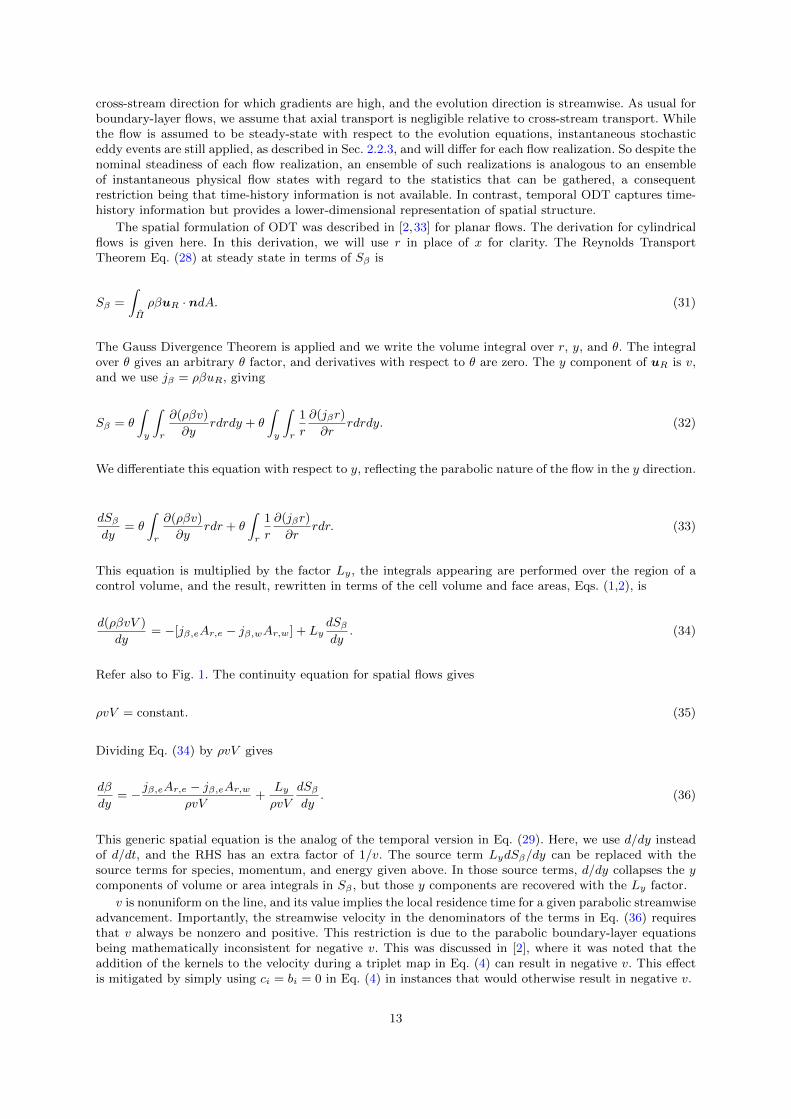
cross-stream direction for which gradients are high, and the evolution direction is streamwise. As usual forboundary-layer flows, we assume that axial transport is negligible relative to cross-stream transport. Whilethe flow is assumed to be steady-state with respect to the evolution equations, instantaneous stochasticeddy events are still applied, as described in Sec. 2.2.3, and will differ for each flow realization. So despite thenominal steadiness of each flow realization, an ensemble of such realizations is analogous to an ensembleof instantaneous physical flow states with regard to the statistics that can be gathered, a consequentrestriction being that time-history information is not available. In contrast, temporal ODT captures time-history information but provides a lower-dimensional representation of spatial structure.

The spatial formulation of ODT was described in [2,33] for planar flows. The derivation for cylindricalflows is given here. In this derivation, we will use r in place of x for clarity. The Reynolds TransportTheorem Eq. (28) at steady state in terms of Sβ is

Sβ =

∫Π

ρβuR · ndA. (31)

The Gauss Divergence Theorem is applied and we write the volume integral over r, y, and θ. The integralover θ gives an arbitrary θ factor, and derivatives with respect to θ are zero. The y component of uR is v,and we use jβ = ρβuR, giving

Sβ = θ

∫y

∫r

∂(ρβv)

∂yrdrdy + θ

∫y

∫r

1

r

∂(jβr)

∂rrdrdy. (32)

We differentiate this equation with respect to y, reflecting the parabolic nature of the flow in the y direction.

dSβdy

= θ

∫r

∂(ρβv)

∂yrdr + θ

∫r

1

r

∂(jβr)

∂rrdr. (33)

This equation is multiplied by the factor Ly, the integrals appearing are performed over the region of acontrol volume, and the result, rewritten in terms of the cell volume and face areas, Eqs. (1,2), is

d(ρβvV )

dy= −[jβ,eAr,e − jβ,wAr,w] + Ly

dSβdy

. (34)

Refer also to Fig. 1. The continuity equation for spatial flows gives

ρvV = constant. (35)

Dividing Eq. (34) by ρvV gives

dβ

dy= − jβ,eAr,e − jβ,eAr,w

ρvV+

LyρvV

dSβdy

. (36)

This generic spatial equation is the analog of the temporal version in Eq. (29). Here, we use d/dy insteadof d/dt, and the RHS has an extra factor of 1/v. The source term LydSβ/dy can be replaced with thesource terms for species, momentum, and energy given above. In those source terms, d/dy collapses the ycomponents of volume or area integrals in Sβ , but those y components are recovered with the Ly factor.

v is nonuniform on the line, and its value implies the local residence time for a given parabolic streamwiseadvancement. Importantly, the streamwise velocity in the denominators of the terms in Eq. (36) requiresthat v always be nonzero and positive. This restriction is due to the parabolic boundary-layer equationsbeing mathematically inconsistent for negative v. This was discussed in [2], where it was noted that theaddition of the kernels to the velocity during a triplet map in Eq. (4) can result in negative v. This effectis mitigated by simply using ci = bi = 0 in Eq. (4) in instances that would otherwise result in negative v.

13

2.4.2 Solution approaches

The temporal or spatial evolution equations are ordinary differential equations (ODEs) at each grid cell.Three solvers are implemented: a first-order explicit Euler method, a first-order semi-implicit method usedfor treating stiff chemistry, and a second-order Strang splitting method [50] also used for stiff chemistry. Thesemi-implicit method uses CVODE [8] to advance the coupled ODEs in a given cell. Each cell is integratedsequentially. Chemical source terms are treated implicitly, while mixing terms are treated explicitly andare fixed at the values at the beginning of the step.

Continuity is imposed as follows. We focus here on reacting gas flows with variable temperature, compo-sition, and density. In the temporal formulation, the cell sizes ∆xo and densities ρo are recorded before eachadvancement step. The temporal evolution ODEs are then advanced one step. Temperature is computedfrom the thermodynamic state, and density ρf is then computed from the ideal gas law. The cell sizes atthe end of the step are then calculated by imposing continuity: ∆xf = ρo∆xo/ρf . Cell face positions arethen computed using ∆xf as previously described in Sec. 2.3. The spatial formulation treatment is similar,but the pre-step velocity vo is also recorded, and Eq. (35), ∆xf = ρovo∆xo/(ρfvf ), is used, where vf isthe post-step velocity computed from the momentum equation.

For all solution approaches, the system of ODEs in each grid cell is advanced with a step size set belowthe diffusive stability limit, computed as the smallest step required for all ODEs over all grid cells.

2.5 Discussion

The finite-volume form of these equations is convenient for solution. The equations are well-behaved at allgrid positions in planar, cylindrical, and spherical geometries. This contrasts the differential form of theequations, which have singularities that require special treatment at the origin for cylindrical and sphericalgeometries due to division by the local radial position.

Here, the only issue is that cell face areas decrease to zero as we approach the origin. As a result,transport across that face tends toward zero, effectively decoupling the two halves of the domain. For cellfaces at or very close to the origin, a zero flux boundary condition is implied. (Technically, the unsteady fluxcan be nonzero but since it multiplies a zero area, the flow is also zero.) This can result in zero gradientswith discontinuous profiles at the origin.

This effect is corrected during mesh management operations by ensuring that the origin is nearly inthe center of the cell containing it so that the flows through either side of that cell are not artificiallyimbalanced due to the face locations. In any case, eddy-induced transport across the origin under theturbulent conditions of interest are far greater than molecular-diffusive fluxes, so there is no significantbarrier to transport across the origin irrespective of diffusive transport mitigation procedures.

One subtlety in the cylindrical and spherical formulations is that the equations include only one-dimensional, line-oriented transport. However, the formulation is nominally axisymmetric; hence solutionon both sides of zero seems redundant. This would be true if we were only solving the evolution equa-tions. The addition of the eddy events breaks the symmetry. We model a turbulent flow with instantaneousasymmetry and eddies that can cross the centerline. The evolution equations can then be thought of asprescribing distinct but coupled time histories of radial property profiles for positive and negative x (radiusr), respectively.

3 Results

This section presents results for three demonstration cases of the cylindrical ODT formulation: a temporalpipe flow, a round spatial jet, and a round spatial jet flame. Mesh resolution is performed as discussed atlength in [33]. Grid density factors (defined in [33]) of 30 and 80 were used for the jet cases and the pipe flowcases, respectively. Grid resolution studies that were performed gave results that were grid-independent.The smallest cell size used in the round jet and jet flame cases were 20 µm, and 64 µm, respectively. Pipeflow simulations are performed with (∆r+)min = 0.333. Time step sizes for the jets and pipe simulations are0.2 and 0.5, respectively, multiplied by the diffusive stability limit 1

2 (∆x2/Γ )min, where Γ the diffusivityof a given transported scalar.

14

(a) (b)

100 101 102 103

y+

0

10

20

30

40

50v

+

Re = 550Re = 1000Re = 2000

DNSTMB

TMAPTMB

100 101 102 103

y+

0

2

4

6

8

v+ rm

s

Re = 550Re = 1000Re = 2000

DNSTMB

TMAPTMB

Fig. 6 ODT simulations and DNS experiments of streamwise mean (a) and RMS (b) velocity profiles at three Reynoldsnumbers. Cases TMA and PTMB are only shown for Reτ = 550.

3.1 Pipe flow

We present results for incompressible pipe flow simulations using the temporal, cylindrical ODT formulation.Results for three different friction Reynolds numbers Reτ = 550, 1, 000, 2, 000 are compared to DNS resultsfrom Khoury et al. [26] (Reτ = 550, 1, 000) and Chin et al. [7] (Reτ = 2, 000). Simulation results wereproduced using a pipe diameter of D = 2.0 m and flow density of 1.0 kg m−3. For fully developed pipe flow,it is possible to estimate the value of a constant mean pressure gradient driving the flow based on the valueof the friction velocity, the pipe radius and the density. Friction velocity values of 1 (Reτ = 550, 1, 000) and2 m s−1 (Reτ = 2, 000) were assumed and used to calculate the mean pressure gradient driving the flow.Simulation results achieving statistical convergence for the friction velocity were verified afterwards as acheck on the input parameters. The simulations used initial conditions with constant velocity profiles. Thesimulations were run to a developed flow state, after which simulation data were gathered until statisticalconvergence for the root mean square (RMS) velocity difference from the mean profiles occurred. The totalnormalized run time trun/τpipe = trunu/D was 20,200, 25,070, and 28,140 for Reτ = 550, 1,000, and 2,000,respectively, where u is the average velocity and D is the pipe diameter.

The simulations were performed with parameters of C = 5 and Z = 350 for the temporal ODTformulation. Additionally, a restriction was imposed on the eddy size range by selecting eddies only up toa maximum normalized size of Le,max/D = 1/3. This restriction limits the eddy size by construction, asopposed to the large-eddy suppression mechanism commonly used in ODT simulations [27,48]. The valuesof C, Z, and Le,max/D were adjusted to give good agreement of the ODT results compared to the DNS.Schmidt et al. [48] showed that higher Z results in the buffer-layer being located further from the wall;increasing C results in a lower slope of the mean streamwise velocity in the log-layer; and higher Le,max/Dgives a smaller mean streamwise velocity in the wake region.

Figure 6(a) results of the mean streamwise velocity profiles in wall units for each of the three Reτconsidered. The profiles are shifted vertically by 10 and 20 units in the figure for presentation. The Reτ =550 case shows a comparison of the TMA, TMB and the hybrid planar/cylindrical approach of the TMBeddy event implementation (PTMB). As seen in the figure, the differences between TMA, TMB, and PTMBare negligible, and so were not considered for the higher Reτ cases. The agreement between the ODT andDNS for the mean velocity is excellent for all three Reτ values.

Figure 6(b) shows the streamwise root mean square (RMS) velocity profiles for each Reτ . These profilesare shifted vertically by 2 and 4 units in the figure for presentation. The ODT RMS velocity profilesdeviate from the DNS more strongly than the mean velocity profiles, with the ODT value at the peakapproximately 20% lower than the DNS. The qualitative shape of the profiles, however, is the same asexpected from previous ODT channel flow simulations performed with the planar formulation [38,33]. Thesmall double peak structure of the ODT was described in [33] and arises from alignment of the triplet mapimages in the near-wall region. The slight depression between the ODT peaks aligns with the DNS peak,resulting in a larger difference between the RMS profiles than an extrapolation of the surrounding ODT

15

(a) (b) (c)

0 20 40 60 80 100y/D

0

5

10

15

20

25v 0

/vcL

ODTEXPFit

0.00 0.05 0.10 0.15 0.20 0.25r/(y y0)

0.00.20.40.60.81.01.2

v/v c

L

y=50Dy=70Dy=90DEXP

0.00 0.05 0.10 0.15 0.20 0.25r/(y y0)

0.00.10.20.30.40.50.6

v rm

s/vcL

y=50Dy=70Dy=90DEXP

Fig. 7 Round jet results for TMB: (a) mean axial velocity along the centerline versus downstream location; (b) radialprofiles of mean axial velocity at three downstream locations; (c) root mean square (RMS) radial profiles of streamwisevelocity at three downstream locations.

profiles to the peak region would give. As for the mean profiles, the differences between TMA, TMB, andPTMB for the RMS velocity profiles are negligible. Small differences appear only for the RMS profiles nearthe centerline. We expect this because of the eddy timescale behavior seen in Fig. 5

A more complete ODT analysis of turbulent pipe and channel flows in both temporal and spatialformulations, including turbulent kinetic energy budgets, is presented in [36].

3.2 Round jet

The new cylindrical ODT formulation is demonstrated in a nonreacting round turbulent jet. Results arecompared to the experimental data of Hussein et al. [19]. The jet consists of air issuing into air through a1 in (0.0254 m) diameter duct. The jet exit velocity is 56.2 m s−1 and is well-approximated by a top-hatprofile. The reported Reynolds number is 95,500, where Re = Dv0/ν, and D is the jet exit diameter, v0is the jet exit velocity, and ν is the kinematic viscosity. The ODT simulations use the same diameter andvelocity, but a kinematic viscosity of 1.534×10−5 m2 s−1, giving a Reynolds number of 93,056. The initialvelocity profile in the ODT simulations is a modified top-hat profile in which a hyperbolic tangent functionof width δ = 0.1D is used on either side of the jet to smooth the transition between the jet and the freestream:

v(x) = vmin +∆v · 1

2

(1 + tanh

(2

δ(x− xc1)

))· 1

2

(1 + tanh

(2

δ(xc2 − x)

)). (37)

Here, xc1 and xc2 are the center locations of the tanh transition, −D/2 and D/2, respectively. In thespatial formulation of ODT, the streamwise velocity must be positive everywhere on the line due to vin the denominator on the right hand side of the evolution equations (see Sec. 2.4.1). As such, a smallvmin = 0.1 m s−1 is added uniformly to the velocity profile. ∆v is taken to be the jet velocity of 56.2 m s−1.

ODT simulations were performed using the TMB triplet map with parameters C = 5.25, βles = 3.5, andZ = 400. The value of Z is the same as the spatial simulations in [39] and was not adjusted. The values ofC and βles were adjusted to give good agreement of the jet evolution with the experimental data. Note thevery close agreement of the C and Z parameters here to the optimal values used for the pipe flow simulationswhere C = 5 and Z = 350. This illustrates a level of robustness in the ODT parameters between the twoconfigurations and suggests that intermediate values could be successfully applied in both configurations.The pipe flow is sensitive to Z, as noted above, but the jet is not, so Z = 350 would be preferred. Figure7 shows results of the simulations. Here, 1024 independent ODT realizations were performed and resultswere ensemble averaged. All quantities are normalized consistent with jet similarity scaling. Downstreamlocations are normalized by the jet diameter D, and radial locations are normalized by (y − y0) where yis the downstream location and y0 = 4D is the virtual origin used in [19]. In the figure, v0 is the jet exitvelocity and vcL is the local mean axial centerline velocity. Here, r is used to denote both the experimentalradial location and the ODT line position x.

Figure 7(a) shows v0/vcL versus y/D; the similarity scaling gives a nominally linear profile where vdecays as 1/y. The ODT simulation compares very well with the stationary wire data in [19] after an initialinduction period for y/D < 20. The dashed line in the plot is the linear curve fit reported by Hussein et

16

(a) (b) (c)

0 20 40 60 80 100y/D

0

5

10

15

20

25v 0

/vcL

ODTEXPFit

0.00 0.05 0.10 0.15 0.20 0.25r/(y y0)

0.00.20.40.60.81.01.2

v/v c

L

y=50Dy=70Dy=90DEXP

0.00 0.05 0.10 0.15 0.20 0.25r/(y y0)

0.00.10.20.30.40.50.6

v rm

s/vcL

y=50Dy=70Dy=90DEXP

Fig. 8 Round jet results for TMA: (a) mean axial velocity along the centerline versus downstream location; (b) radialprofiles of mean axial velocity at three downstream locations; (c) root mean square (RMS) radial profiles of streamwisevelocity at three downstream locations.

al. Figure 7(b) shows radial profiles of the mean axial velocity normalized by the local centerline value.Profiles at three axial locations, 50D, 70D, and 90D, are shown. The experimental data points shownare the laser Doppler anemometer (LDA) data in [19]. The ODT results show a similarity collapse of thedata at r/(y − y0) < 0.1, but some spread in the profiles at higher r/(y − y0), with the simulation resultsrelaxing towards the experimental values with downstream distance. Figure 7(c) shows radial profiles ofthe axial root mean square (RMS) velocity normalized by the local centerline velocity at the same threepositions. Here again, the profiles tend to relax towards the experimental (LDA) data at higher r/(y − y0)with downstream distance.

The quantitative agreement of vrms velocity is generally good, especially for r/(y−y0) > 0.03. At lowervalues, near the centerline, the ODT vrms increases, whereas the experimental data decrease slightly. Weattribute this to the so-called centerline anomaly of the cylindrical ODT formulation due to the geometricstretching associated with the cylindrical triplet maps. This stretching was shown in Figs. 2 and 3. In fact,the motivation for developing TMB was to minimize the degree of this geometric stretching. The stretchingeffect was present for both maps TMA and TMB, but it is largest near the centerline, where curvature islarge. With increasing distance from the centerline, that is, for large distances compared to the eddy size,the geometric stretching effect becomes negligible for both maps, and they both approach the planar limit.

For comparison to the ODT results with TMB shown in Fig. 7, similar simulations were performed withTMA, and corresponding results are shown in Fig. 8. Here, βles and Z are the same as for the previouscase with TMB, but C = 7. Again, we see good agreement for the centerline velocity decay in Fig. 8(a).A somewhat better similarity collapse than for TMB occurs in the radial velocity profiles, though they areslightly lower than the experimental data at r/(y − y0) < 0.13 and slightly higher than the experimentaldata at r/(y − y0) > 0.13. The vrms profiles also show strong similarity scaling. Compared with TMB,however, the simulations show a much higher centerline anomaly, and the vrms profile departs from theexperiments much further from the centerline and has a higher rise in the region r/(y − y0) < 0.05.

It is worth noting that the vrms profile depends somewhat on the ODT parameters selected. Hewson andKerstein [15] demonstrated that mean centerline values of mixture fraction were insensitive to C and βlesprovided their ratio was kept constant. In these simulations, however, higher values of RMS fluctuationswere observed at lower values of βles. Figure 9 shows results for TMA similar to those in Fig. 8 with varyingC and βles. Each of the three cases has C/βles = 2, with C = 7, 5, and 3. Plots (b) and (c) show axiallocation 70D. There is very little variation of the mean centerline velocity decay for the three cases. Theradial profiles of the mean streamwise velocity are also very close, but they decrease somewhat in valuewith decreasing C for intermediate r/(y− y0) values. In contrast, the vrms profiles are strongly dependenton the values of C and βles for a constant C/βles ratio, with increasing vrms for decreasing βles. Theseresults are consistent with those presented for mixture fraction by Hewson and Kerstein [15]. In Fig. 9(c),the centerline anomaly appears to increase with decreasing βles, and the departure from the data occursfurther from the origin with increasing βles. That is, the simulations fit more of the data over a wider radialrange at lower values of βles.

The centerline anomaly tends to increase the velocity fluctuations near the centerline. This is primarilydue to the effect of the cylindrical triplet maps on the eddy rate, as shown in Fig. 5. To minimize the effectof the centerline anomaly, the planar evaluation of τ−1

e described in Sec. 2.2.4 (PTMB) is used. Resultsare shown in Fig. 10. Here, C = 7, βles = 3.5, and Z = 400. The centerline velocity decay and radial

17

(a) (b) (c)

0 20 40 60 80 100y/D

0

5

10

15

20

25v 0

/vcL

C = 7, les = 3.5C = 5, les = 2.5C = 3, les = 1.5EXP

0.00 0.05 0.10 0.15 0.20 0.25r/(y y0)

0.00.20.40.60.81.01.2

v/v c

L

C = 7, les = 3.5C = 5, les = 2.5C = 3, les = 1.5EXP

0.00 0.05 0.10 0.15 0.20 0.25r/(y y0)

0.00.10.20.30.40.50.6

v rm

s/vcL

C = 7, les = 3.5C = 5, les = 2.5C = 3, les = 1.5EXP

Fig. 9 Round jet results for TMA for three cases: (a) mean axial velocity along the centerline versus downstream location;(b) radial profiles of mean axial velocity at y = 70D; (c) root mean square (RMS) radial profiles of streamwise velocityy = 70D.

(a) (b) (c)

0 20 40 60 80 100y/D

0

5

10

15

20

25

v 0/v

cL

ODTEXPFit

0.00 0.05 0.10 0.15 0.20 0.25r/(y y0)

0.00.20.40.60.81.01.2

v/v c

L

y=50Dy=70Dy=90DEXP

0.00 0.05 0.10 0.15 0.20 0.25r/(y y0)

0.00.10.20.30.40.50.6

v rm

s/vcL

y=50Dy=70Dy=90DEXP

Fig. 10 Round jet results for the case of planar evaluation of τ−1e (PTMB): (a) mean axial velocity along the centerline

versus downstream location; (b) radial profiles of mean axial velocity at three downstream locations; (c) root mean square(RMS) radial profiles of streamwise velocity at three downstream locations.

profiles show good agreement, as with the previous cases, with a slight improvement in the radial velocityprofile. The vrms profiles are significantly improved along the centerline compared to TMA and TMB. Thecenterline anomaly is not completely removed, however, since implemented eddies are still subject to thegeometric distortion of the TMB map, whose influence is felt by the τ−1

e calculation for subsequent eddyevents.

3.3 Round jet flame

The new cylindrical ODT formulation is demonstrated in a round, reacting, turbulent jet flame. Resultsare compared to the experimental DLR-A flame of Meier et al. [37,1]. Heat release and temperature-and composition-dependent transport and thermodynamic properties are key characteristics of this flow.This canonical flame configuration has been used extensively to study and validate turbulent combustionmodels. Pitsch [42] studied differential diffusion effects in this flame using a classical unsteady flameletmodel. Lindstedt and Ozarivsky [35] investigated it using a joint PDF approach, while Wang and Pope[53] used an LES/PDF model combined with a flamelet/progress-variable (FPV) model. Fairweather andWoolley [11] studied several chemical mechanisms using the DLR flame and a first order conditional momentclosure (CMC) model, and Lee and Choi [30,29] studied NO emissions using an Eulerian particle flameletmodel. These studies consisted of computational fluid dynamics (CFD) simulations with subgrid modelingof the turbulent combustion process. In contrast, ODT is a low-dimensional representation of the entireflow, not just the subgrid scales. Previous ODT studies of turbulent jet flames have employed the temporalplanar formulation, so we expect that the model may improve with a spatial cylindrical formulation thatmore closely matches the experimental configuration.

The DLR-A fuel stream is mixture of 22.1% CH4, 33.2% H2, and 44.7% N2 (by volume) that issuesinto dry air. The fuel stream exits a nozzle with an inner diameter of 8 mm at a mean exit velocity of 42.2

18

(a) (b) (c)

0 20 40 60 80 100y/D

0102030405060

v (m

/s) CL

RMS

ODTEXP

0 20 40 60 80 100y/D

0.00.20.40.60.81.01.2

CL

RMS

ODTEXP

0 20 40 60 80 100y/D

0

500

1000

1500

2000

2500

T (K

) CL

RMS

ODTEXP

Fig. 11 DLR jet flame results for TMB: (a) mean axial velocity and RMS velocity along the centerline versus downstreamlocation; (b) mean axial mixture fraction and RMS mixture fraction along the centerline versus downstream location; (c)mean axial temperature (K) and RMS temperature (K) along the centerline versus downstream location.

m s−1. The coflowing air stream issues from a nozzle of diameter 140 mm at a velocity of 0.3 m s−1. Thereported Reynolds number is 15,200.

The ODT simulation uses these diameters and the experimentally reported velocity profile at the jetexit. Whereas in the nonreacting case, a small velocity was added uniformly to the profile, no velocityaddition is needed here because of the slow-moving coflow air stream present alongside the reacting jet.The ODT simulation includes the buoyant source term but not the streamwise pressure gradient in Eq. (25).The fuel was diluted with N2 in the experimental flame to minimize radiative heat losses, and radiation isignored in the simulation. This flame has a low Reynolds number and the combustion chemistry proceedsquickly. The ODT simulation transports the following species: O2, N2, CH4, H2, H2O, CO2. Reactions areassumed to proceed to products of complete combustion:

CH4 + 2 O2 −−→ CO2 + 2 H2O, (38)

H2 +1

2O2 −−→ H2O, (39)

and simple, fast reaction rates are applied. These assumptions are not reasonable for the DLR-A flame.The primary purpose of these simulations is to illustrate ODT in a reacting jet with variable propertiesand heat release.

ODT simulations were performed using the TMB triplet map with parameters C = 20, βles = 17, andZ = 400. The values of C and βles were adjusted to give good agreement of the jet evolution with theexperimental data, while the value of Z was taken as the same value as for the jet in Sec. 3.2. Results ofthe simulation are presented in Figs. 11 and 12. 1000 independent flow realizations were performed and theresults ensemble averaged. Downstream distance y, and radial position r are normalized by the jet diameterD.

Figure 11 shows ODT and experimental axial mean and RMS profiles along the jet centerline for (a)axial velocity, (b) mixture fraction ξ, and (c) temperature T . The ODT results track the experimental datawell for all three variables. The centerline temperature is about 100 K above the experiments at the peakat y/D = 60. This small difference is likely due to thermal radiation and differences between equilibriumproducts and products of complete combustion.

The centerline velocity has a fast initial decrease due to diffusion. There is a delay in the ODT RMSprofiles on the centerline before the eddies occur near y/D = 7. This delay is due to the elapsed time modelfor large eddy suppression discussed in Sec. 2.2.2 so that, initially, only small eddies occur in the shear layerson the jet edges away from the centerline. The experimental RMS measurements also reflect non-vortical“flapping” of the jet [13,4] that ODT is not able to capture. Centerline RMS agreement is good for allvariables for y/D > 25. Note especially that the ODT captures the dip in the RMS temperature profilenear the peak temperature at y/D = 60. This decrease in the RMS fluctuations is due to the combinedeffects of decreased density and increased viscosity at high temperature, which decrease the local Reynoldsnumber.

Radial profiles of mean mixture fraction and temperature for the jet are shown in Fig. 12 at six down-stream locations. The ODT and experimental profile widths are in good agreement, with the ODT beingslightly narrower. The peak temperature values in the “wings” occur at the flame surfaces, and the ODTvalues overpredict the experiments. This could be due to radiative losses and finite-rate chemistry effects,which are not modeled here.

19

(a) (b)

0.00.20.40.60.81.0 y/D = 80

CLEXPODT

0.000.050.100.15y/D = 80

RMS

0.00.20.40.60.81.0 y/D = 60

0.000.050.100.15y/D = 60

0.00.20.40.60.81.0 y/D = 40

0.000.050.100.15y/D = 40

0.00.20.40.60.81.0 y/D = 20

0.000.050.100.15y/D = 20

0.00.20.40.60.81.0 y/D = 10

0.000.050.100.15y/D = 10

15 10 5 0 5 10 15r/D

0.00.20.40.60.81.0 y/D = 5

15 10 5 0 5 10 15r/D

0.000.050.100.15y/D = 5

5001000150020002500

T (K

)

y/D = 80

CLEXPODT

0100200300400500

T (K

)

y/D = 80

RMS

5001000150020002500

T (K

)

y/D = 60

0100200300400500

T (K

)

y/D = 60

5001000150020002500

T (K

)

y/D = 40

0100200300400500

T (K

)

y/D = 40

5001000150020002500

T (K

)

y/D = 20

0100200300400500

T (K

)

y/D = 20

5001000150020002500

T (K

)

y/D = 10

0100200300400500

T (K

)

y/D = 10

15 10 5 0 5 10 15r/D

5001000150020002500

T (K

)y/D = 5

15 10 5 0 5 10 15r/D

0100200300400500

T (K

)

y/D = 5

Fig. 12 Radial mean and RMS profiles for mixture fraction (a) and temperature (b) for the DLR jet flame.

The RMS temperature and mixture fraction profiles are also shown in Fig. 12. While the fluctuations areaccurate on the centerline, the ODT underpredict the experiments away from the centerline. This dependson the ODT parameters chosen, as shown in Fig. 9. The very large difference in the RMS profiles at lowy/D is simply due to the delay in the ODT eddies noted previously and the possible flapping contributionthat ODT does not capture. The centerline anomaly can also be seen in the RMS profiles for y/D ≥ 40,but the magnitude is somewhat smaller than was observed in the nonreacting jet simulations.

Simulations were also performed using the PTMB model. Optimal parameters were close to those forthe TMB case: C = 18, βles = 18, and Z = 400. The results are so similar to the TMB case that we do notinclude them here. As expected, the centerline anomaly is decreased, consistent with the behavior of thenonreacting jet, shown previously.

The difference in the optimal parameters for the reacting and nonreacting jets for the TMB model aresurprising. Z is the same for both simulations, but C = 5.25, βles = 3.5, C/βles = 1.5 for the nonreactingjet, and C = 20, βles = 17, C/βles = 1.18 for the DLR-A flame. Both jets had reasonably good agreementwith the experiments. We ran the DLR-A flame with the nonreacting jet parameters. The results for thecenterline mixture fraction are shown in Fig. 13. The nonreacting parameters result in faster centerlinedecay and higher RMS velocity fluctuations.

Differences in the required parameters for the reacting jet may be expected due to effects of variabledensity and viscosity. However, we expect flow dilatation to have a significant impact. Hewson and Kerstein[15] discussed the effect of flow dilatation on ODT evolution in some detail and the results we observe hereare consistent with their analysis. In ODT, flow dilatation occurs only in the radial direction and directlyaffects only flow length scales. Real dilatation at low Mach numbers is three dimensional, and affects bothlength scales and velocity, with the effects of increasing rates of dissipation (which scale as u3/l), andpushing the flow downstream. This is seen in Fig. 13, where the centerline experimental mixture fractionsfall off more slowly than for ODT with the nonreacting parameter values. This is counteracted in ODTwith a lower C/βles ratio, effectively reducing the mixing rate and shifting the ODT mixture fraction curve

20

0 20 40 60 80 100y/D

0.00.20.40.60.81.01.2

CLRMS

ODT, C = 5.25, les = 3ODT, C = 20, les = 17EXP

Fig. 13 Centerline mean and RMS mixture fraction for the DLR-A flame with nonreacting jet parameters, and optimizedparameters.

downstream. Figure 9 showed that RMS fluctuations were lower for higher values of C for a given C/βlesratio. Hence, the higher C value used in the tuned DLR-A case also tends to reduce the high RMS valuesseen in Fig. 13 at y/D < 35.

4 Conclusions

A new formulation of the ODT model in cylindrical and spherical coordinates was developed and presented.A Lagrangian finite-volume method utilizing an adaptive mesh was used, and the model is formulated forboth temporal and spatial variants.

ODT resolves a full range of length and time scales in a physical space coordinate. This unique aspectof the model allows high fidelity investigation into a wide range of complex multi-scale turbulent flows.DNS is the only simulation approach that can resolve all continuum scales in three dimensions. But DNSis computationally expensive, limiting the number of simulations that can be performed and the accessibleparameter space (e.g., the range of Reynolds numbers available). ODT can be used to study flows outside ofthe parameter space available to DNS, and is computationally efficient enough to allow extensive parametricstudy. However, ODT models turbulent advection, and is not able to directly capture multi-dimensionalflow structures or transport. ODT also includes model parameters that must be adjusted for specific flows.Hence, ODT is most reliable when used in conjunction with experimental data, or when experimental datais used as a basis for calibrating ODT that is subsequently used in extrapolative studies.

Previous ODT simulations were limited to planar configurations, but many detailed experiments ofturbulent flows, especially jets and jet flames, are axi-symmetric (cylindrical). While temporal planar ODTcan be reasonably applied to cylindrical jets due to similar scaling behaviors, this is not ideal due todifferences in implied fluid time-history profiles (important for particle studies, soot formation, and flame-extinction/reignition, for example), and geometric effects, such as obtaining correct mass flow rates inpiloted flames. Improved consistency in the geometric configuration between ODT and experiments reducesuncertainties in the source of discrepancies.

The cylindrical and spherical formulations were presented for the unsteady evolution equations of mass,momentum, energy and species. Some extensions and corrections to the treatment of constrained volumeflows with variable density in [33] were given. For flows with dilatation, while planar flows allow the centerof the fluid expansion to be fixed, in cylindrical and spherical flows we fix the radial origin.

Turbulent advection is modeled as instantaneous eddy events implemented using the triplet map. Incylindrical and spherical coordinates, geometric stretching occurs in the three map images. Two tripletmap variants were presented, TMA and TMB. In TMA, each map segment has the same volume, resultingin each segment having different radial lengths. In TMB, each map segment is given the same radialsegment length, resulting segments having different volumes. The geometric stretching is strongest near theorigin and is due to the volume dependence on radial location. The stretching affects the eddy timescale,resulting in a so-called centerline anomaly, that was manifested as an increase in velocity fluctuations near

21

the centerline in the jet configuration studied. The TMB map performed better than TMA. A hybridplanar-TMB (PTMB) map was also presented and this further reduced the centerline anomaly.

Three flow configurations were studied: a temporal pipe flow, a spatial nonreacting jet at high Reynoldsnumber, and a spatial reacting jet flame at relatively low Reynolds number. The jet flame illustrateseffects of variable density and viscosity, including dilatational effects, which had a significant impact onthe required ODT parameters. The cylindrical ODT formulation was found to capture key features of DNSresults for pipe flow, and experimental results were reproduced with quantitative accuracy in most instancesfor the nonreacting and reacting jets, which are considered to be an improvement over previous temporalformulations, though this is not explicitly investigated here. The TMA, TMB, and PTMB maps gave nearlyidentical results for the pipe flow, where the key dynamics are near-wall away from the centerline wherestretching effects are important. The ODT C and Z parameters were nearly the same for the jet (TMB)and the pipe flow, illustrating a degree of robustness of the ODT parameters across configurations.

While spherical ODT was formulated here, the focus was on cylindrical flows. Application of ODT tospherical flows, will be the subject of future study. The brief pipe flow results presented here were used forillustration. A more comprehensive and detailed study of pipe flow is underway [36], that includes the spatialand temporal ODT formulations, and analysis of turbulent kinetic energy budgets. Further applications ofthe cylindrical ODT formulation to jet flames are also underway.

Appendix A: ODT time advancement procedure

The overall advancement scheme for temporal ODT is outlined here, including some algorithmic detailsrelated to the time advancement. Formally, the outcome of time advancement of any property c from timet = 0 to time t∗ can be expressed as

c(x, t) = T [tn, t∗]E(xn, ln) · · ·T [tj , tj+1]E(xj , lj)T [tj−1, tj ] · · ·E(x2, l2)T [t1, t2]E(x1, l1)T [0, t1]c(x, 0), (40)

where capital letters represent operators. T [tj−1, tj ] denotes time advancement of c(x, tj−1) from tj−1 to tj .The equations governing the advancement of the flow and state properties included in present formulationare shown in Sec. 2.3. E(xj , lj) denotes an eddy event that induces an instantaneous change c(x, tj) →c′(x, tj), where xj is the left edge of the jth eddy, lj is its length, and tj is its time of occurrence. Theprocedure for sampling these eddy attributes is described below. n is the number of eddy events that occurduring [0, t∗].

A key feature of the sampling procedure is that it samples candidate events that are then subject toacceptance or rejection based on a computed acceptance probability Pa. Before explaining these details, wenote their consequences with regard to the sequence of operations shown in Eq. (40).

Equation (40) represents the operations that can modify property c. Candidate events that are rejectedhave no such effect, so they are not included in that representation. The numerical algorithm thereforerequires a more detailed representation. The arguments of T and E can now be omitted for brevity; thefull notation can be inferred from Eq. (40). Denoting a rejected candidate event by R, a representativesequence of operations during some subinterval of a simulated realization can be expressed as

· · · TRTRTE TRTRTRTRTE TRTRTRT · · · .

The greater frequency of rejections than acceptances is intended to illustrate the smallness of Pa, which isexplained below.

The time interval between candidate events (R or E) is extremely small for two reasons. First, undertypical conditions, the time between eddies containing a given location is comparable to the diffusion timescale that corresponds to the typical eddy size. The smallest (Kolmogorov) eddies are the most numerousand hence the typical eddies. Due to their smallness, many of them must occur during some time intervalin order for a given location to be contained in one of them. This implies that the time between eddies ismuch smaller than the diffusion time scale, which, by the same reasoning, is roughly the Kolmogorov timescale, assuming gas-phase conditions.

Second, these considerations apply to the physically occurring (accepted) eddies. As noted, rejectedcandidate eddies are much more frequent, so the time interval between them is commensurately smaller.Therefore, the T operation in the above advancement representation typically acts over a time interval muchsmaller than the maximum permitted by accuracy and stability constraints, which is grossly inefficient.

To remedy this, recall that the event R causes no change of the system state, hence its omission fromEq. (40). Therefore, the occurrence of such an event need not trigger an advancement operation if that

22

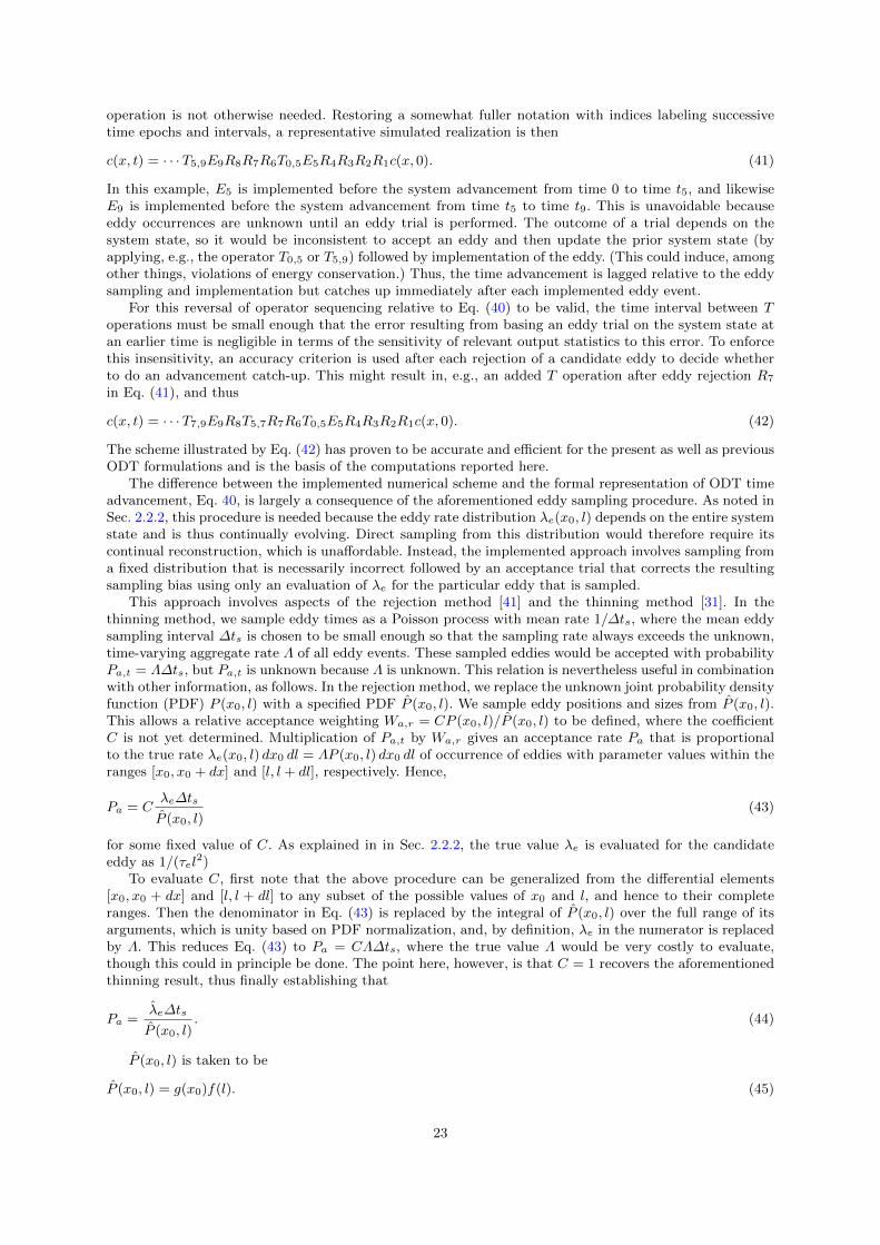
operation is not otherwise needed. Restoring a somewhat fuller notation with indices labeling successivetime epochs and intervals, a representative simulated realization is then

c(x, t) = · · ·T5,9E9R8R7R6T0,5E5R4R3R2R1c(x, 0). (41)

In this example, E5 is implemented before the system advancement from time 0 to time t5, and likewiseE9 is implemented before the system advancement from time t5 to time t9. This is unavoidable becauseeddy occurrences are unknown until an eddy trial is performed. The outcome of a trial depends on thesystem state, so it would be inconsistent to accept an eddy and then update the prior system state (byapplying, e.g., the operator T0,5 or T5,9) followed by implementation of the eddy. (This could induce, amongother things, violations of energy conservation.) Thus, the time advancement is lagged relative to the eddysampling and implementation but catches up immediately after each implemented eddy event.

For this reversal of operator sequencing relative to Eq. (40) to be valid, the time interval between Toperations must be small enough that the error resulting from basing an eddy trial on the system state atan earlier time is negligible in terms of the sensitivity of relevant output statistics to this error. To enforcethis insensitivity, an accuracy criterion is used after each rejection of a candidate eddy to decide whetherto do an advancement catch-up. This might result in, e.g., an added T operation after eddy rejection R7

in Eq. (41), and thus

c(x, t) = · · ·T7,9E9R8T5,7R7R6T0,5E5R4R3R2R1c(x, 0). (42)

The scheme illustrated by Eq. (42) has proven to be accurate and efficient for the present as well as previousODT formulations and is the basis of the computations reported here.

The difference between the implemented numerical scheme and the formal representation of ODT timeadvancement, Eq. 40, is largely a consequence of the aforementioned eddy sampling procedure. As noted inSec. 2.2.2, this procedure is needed because the eddy rate distribution λe(x0, l) depends on the entire systemstate and is thus continually evolving. Direct sampling from this distribution would therefore require itscontinual reconstruction, which is unaffordable. Instead, the implemented approach involves sampling froma fixed distribution that is necessarily incorrect followed by an acceptance trial that corrects the resultingsampling bias using only an evaluation of λe for the particular eddy that is sampled.

This approach involves aspects of the rejection method [41] and the thinning method [31]. In thethinning method, we sample eddy times as a Poisson process with mean rate 1/∆ts, where the mean eddysampling interval ∆ts is chosen to be small enough so that the sampling rate always exceeds the unknown,time-varying aggregate rate Λ of all eddy events. These sampled eddies would be accepted with probabilityPa,t = Λ∆ts, but Pa,t is unknown because Λ is unknown. This relation is nevertheless useful in combinationwith other information, as follows. In the rejection method, we replace the unknown joint probability densityfunction (PDF) P (x0, l) with a specified PDF P (x0, l). We sample eddy positions and sizes from P (x0, l).This allows a relative acceptance weighting Wa,r = CP (x0, l)/P (x0, l) to be defined, where the coefficientC is not yet determined. Multiplication of Pa,t by Wa,r gives an acceptance rate Pa that is proportionalto the true rate λe(x0, l) dx0 dl = ΛP (x0, l) dx0 dl of occurrence of eddies with parameter values within theranges [x0, x0 + dx] and [l, l + dl], respectively. Hence,

Pa = Cλe∆ts

P (x0, l)(43)

for some fixed value of C. As explained in in Sec. 2.2.2, the true value λe is evaluated for the candidateeddy as 1/(τel

2)To evaluate C, first note that the above procedure can be generalized from the differential elements

[x0, x0 + dx] and [l, l + dl] to any subset of the possible values of x0 and l, and hence to their completeranges. Then the denominator in Eq. (43) is replaced by the integral of P (x0, l) over the full range of itsarguments, which is unity based on PDF normalization, and, by definition, λe in the numerator is replacedby Λ. This reduces Eq. (43) to Pa = CΛ∆ts, where the true value Λ would be very costly to evaluate,though this could in principle be done. The point here, however, is that C = 1 recovers the aforementionedthinning result, thus finally establishing that

Pa =λe∆ts

P (x0, l). (44)

P (x0, l) is taken to be

P (x0, l) = g(x0)f(l). (45)

23

g(x0) is a uniform distribution over the range [0, Ld − l], where Ld is the domain length. Its dependenceon l indicates that l must be sampled before x0. (The range is [0, L] for the case of periodic boundaryconditions.) f(l) is taken to be

f(l) =All2e−2l/l, (46)

where l is the most probable eddy size, as specified by the user, and Al is the PDF normalization constant.

To summarize, we sample an eddy position x0 and size l from P (x0, l) at an eddy occurrence timeevaluated from a Poisson process with mean rate 1/∆ts and accept that eddy with the probability given inEq. (44). ∆ts is adjusted during the simulation to ensure that Pa is always less than unity. The rejectionand thinning methods affect the eddy sampling efficiency, but not the accuracy of the process. The closerPa is to unity, and the better the approximation P ≈ P , the more efficient the method will be. However,the possible system states during a typical realization are so diverse that Pa varies widely for given ∆ts,so to ensure that Pa < 1, ∆ts has to be small enough that Pa is typically very small. As noted above, thishas ramifications with regard to the design of the time advancement scheme. In any case, this approach ismuch faster than directly sampling P (x0, l), which would require it to be continually updated.

Appendix B: Pressure term in the energy equation

The pressure term in Eq. (27) arises in constant or constrained volume ideal gas flows. That term was derivedin [33] for planar flows; the treatment here is similar, but with some extensions and minor corrections. Weconstrain ourselves to a low-Mach number formulation [44]. The pressure term is then

dP

dt= −γP∇ · u+ γPU . (47)

Here, γ = cp/cv = cp/(cp −R/M), where cp and cv are heat capacities (per unit mass), R is the universalgas constant, M is the mean molecular weight, and U is

U =1

ρcpT

(−∇ · q +

∑k

hk(∇ · jk − m′′′k )

)− M

ρ

∑k

1

Mk(∇ · jk − m′′′k ). (48)

In this equation, hk is the enthalpy of species k per unit mass. Equation (47) is integrated over the wholedomain by assuming that P and dP/dt are spatially uniform. This gives

dP

dt=

∫UdV − (URbcARbc − ULbcALbc)

1P

∫1γ dV

. (49)

Here, URbc and ULbc denote velocities of the right and left boundaries; they are normally zero for constantvolume configurations but are retained here for generality. The volume integrals extend over the wholedomain and are evaluated as a summation over cell integrals. See also Eq. (51) below. As before, we assumethat cells have uniform properties.

Given dP/dt, we compute the dilatational cell face velocities for use in the Lagrangian formulation forconstant or constrained volume flows. Equation (47) is solved for ∇ · u and volume integrated over anindividual cell to give an expression for the difference between cell face velocities:

UeAe − UwAw =− 1

γP

dP

dtV +

∫UdV, (50)∫

UdV =1

ρcpT

(−(qeAe − qwAw) +

∑k

hk(jk,eAe − jk,wAw − m′′′k V )

)− (51)

M

ρ

∑k

1

Mk(jk,eAe − jk,wAw − m′′′k V ).

In the evaluation of Eqs. (50, 51), the volume integrals of the divergences of vector quantities were convertedto surface integrals using the Gauss Divergence Theorem; that way, the equations use readily available cellface velocities and fluxes. Using Eqs. (50, 51), any given face velocity can be computed by marching froma known boundary velocity.

24

While dP/dt given in Eq. (49) is used in Eqs. (50, 27), the pressure itself is updated following Motheauand Abraham [40], where the pressure is set by the global gas state using the ideal gas law. The mass onthe line is given by ml =

∫ρdV , where ρ = MP/(RT ). When P is spatially uniform, we obtain

P =mlR∫MT dV

. (52)

Acknowledgements This work was supported by the National Science Foundation under grant number CBET-1403403.

References

1. International workshop on measurement and computation of turbulent nonpremixed flames, URL: http://www.sandia.gov/TNF/DataArch/DLRflames.html

2. Ashurst, W.T., Kerstein, A.R.: One-dimensional turbulence: Variable-density formulation and application to mixinglayers. Physics of Fluids 17, 025,107 (2005)

3. Ashurst, W.T., Kerstein, A.R.: Erratum: One-dimensional turbulence: variable density formulation and application tomixing layers. Physics of Fluids 21-119901, 1 (2009)

4. Binder, G., Favre-Marinet, M.: Some characteristics of pulsating or flapping jets. In: R. Michel, J. Cousteix,R. Houdeville (eds.) Unsteady turbulent shear flows, pp. 370–379. Springer (1981)

5. Cao, S., Echekki, T.: A low-dimensional stochastic closure model for combustion large-eddy simulation. Journal ofTurbulence 9, 1–35 (2008)

6. Cengel, Y.A., Cimbala, J.M.: Fluid Mechanics, 2 edn. McGraw-Hill (2006)7. Chin, C., Monty, J.P., Ooi, A.: Reynolds number effects in DNS of pipe flow and comparison with channels and

boundary layers. Int. J. Heat Fluid Flow 45, 33–40 (2014)8. Cohen, S.D., Hindmarsh, A.C.: CVODE, a stiff/nonstiff ODE solver in C. Computational Physics 10, 138–143 (1996).

http://llnl.gov/casc/sundials/

9. Cook, A.W., Riley, J.J., Kosaly, G.: A laminar flamelet approach to subgrid-scale chemistry in turbulent flows. Com-bustion and Flame 109, 332–341 (1997)

10. Echekki, T., Kerstein, A.R., Dreeben, T.D.: One-dimensional turbulence simulation of turbulent jet diffusion flames:Model formulation and illustrative applications. Combustion and Flame 125, 1083–1105 (2001)

11. Fairweather, M., Woolley, R.: First-order conditional moment closure modeling of turbulent, nonpremixed methaneflames. Combustion and Flame 138, 3–19 (2004)

12. Gastine, T., Wicht, J., Aurnou, J.M.: Turbulent Rayleigh-Benard convection in spherical shells. Journal of FluidMechanics 778, 721–764 (2015)

13. Goldschmidt, V.W., Bradshaw, P.: Flapping of a plane jet. Physics of Fluids 16, 354–355 (1973)14. Goshayeshi, B., Sutherland, J.C.: Prediction of oxy-coal flame stand-off using high-fidelity thermochemical models and

the one-dimensional turbulence model. Proceedings of the Combustion Institute 35, 2829–2837 (2015)15. Hewson, J.C., Kerstein, A.R.: Stochastic simulation of transport and chemical kinetics in turbulent CO/H2/N2 flames.

Combustion Theory and Modelling 5, 669–697 (2001)16. Hewson, J.C., Kerstein, A.R.: Local extinction and reignition in nonpremixed turbulent CO/H2/N2 jet flames. Com-

bustion Science and Technology 174, 35–66 (2002)17. Hewson, J.C., Ricks, A.J., Tieszen, S.R., Kerstein, A.R., Fox, R.O.: Conditional moment closure with differential

diffusion for soot evolution in fire. In: Center for Turbulence Research, Proceedings of the Summer Program (2006)18. Hewson, J.C., Ricks, A.J., Tieszen, S.R., Kerstein, A.R., Fox, R.O.: On the transport of soot relative to a flame:

modeling differential diffusion for soot evolution in fire. In: H. Bockhorn, A. D’Anna, A.F. Sarofim, H. Wang (eds.)Combustion Generated Fine Carbonaceous Particles. KIT Scientific Publishing (2009)

19. Hussein, H.J., Capp, S.P., George, W.K.: Velocity measurements in a high-Reynolds-number, momentum-conserving,axisymmetric, turbulent jet. Journal of Fluid Mechanics 258, 31–75 (1994)

20. Jozefik, Z., Kerstein, A.R., Schmidt, H.: Simulation of shock-turbulence interaction in non-reactive flow and in turbulentdeflagration and detonation regimes using one-dimensional turbulence. Combustion and Flame 164, 53–67 (2016)

21. Jozefik, Z., Kerstein, A.R., Schmidt, H., Lyra, S., Kolla, H., Chen, J.H.: One-dimensional turbulence modeling of aturbulent counterflow flame with comparison to DNS. Combustion and Flame 162, 2999–3015 (2015)

22. Kerstein, A.R.: Linear-eddy modelling of turbulent transport. Part 6. Microstructure of diffusive scalar mixing fields.Journal of Fluid Mechanics 231, 361–394 (1991)

23. Kerstein, A.R.: One-dimensional turbulence: Model formulation and application to homogeneous turbulence, shearflows, and buoyant stratified flows. Journal of Fluid Mechanics 392, 277–334 (1999)

24. Kerstein, A.R., Ashurst, W.T., Wunsch, S., Nilsen, V.: One-dimensional turbulence: Vector formulation and applicationto free shear flows. Journal of Fluid Mechanics 447, 85–109 (2001)

25. Kerstein, A.R., Dreeben, T.D.: Prediction of turbulent free shear flow statistics using a simple stochastic model. Physicsof Fluids 12, 418–424 (2000)

26. Khoury, G., Schlatter, P., Noorani, A., Fischer, P., Brethouwer, G., Johansson, A.: Direct numerical simulation ofturbulent pipe flow at moderately high Reynolds numbers. Flow Turbulence Combust. 91, 475–495 (2013)

27. Krishnamoorthy, N.: Reaction models and reaction state parameterization for turbulent nonpremixed combustion.Ph.D. thesis, The University of Utah (2008)

28. Lackmann, T., Kerstein, A.R., Oevermann, M.: A representative linear eddy model for simulating spray combustionin engines . Submitted to Combustion and Flame, 2017

29. Lee, K., Choi, D.: Analysis of NO formation in high temperature diluted air combustion in a coaxial jet flame usingan unsteady flamelet model. International Journal of Heat and Mass Transfer 52, 1412–1420 (2009)

25

30. Lee, K.W., Choi, D.H.: Prediction of NO in turbulent diffusion flames using eulerian particle flamelet model. Combus-tion Theory and Modelling 12, 905–927 (2008)

31. Lewis, P.A., Shedler, G.S.: Simulation of nonhomogeneous poisson processes by thinning. Naval Res. Logistics Quart.26, 403–413 (1979)

32. Lignell, D.O., Fredline, G.C., Lewis, A.D.: Comparison of one-dimensional turbulence and direct numerical simulationsof soot formation and transport in a nonpremixed ethylene jet flame. Proceedings of the Combustion Institute 35,1199–1206 (2015)

33. Lignell, D.O., Kerstein, A.R., Sun, G., Monson, E.I.: Mesh adaption for efficient multiscale implementation of one-dimensional turbulence. Theoretical and Computational Fluid Dynamics 27, 273–295 (2013)

34. Lignell, D.O., Rappleye, D.: One-dimensional-turbulence simulation of flame extinction and reignition in planar ethylenejet flames. Combustion and Flame 159, 2930–2943 (2012)

35. Lindstedt, R., Ozarovsky, H.: Joint scalar transported PDF modeling of nonpiloted turbulent diffusion flames. Com-bustion and Flame 143, 471–490 (2005)

36. Medina, J., Schmidt, H., Lignell, D.O.: Application of one-dimensional turbulence to incompressible channel and pipeflow . Submitted to Journal of Turbulence, (2017).

37. Meier, W., Barlow, R., Chen, Y.L., Chen, J.Y.: Raman/Rayleigh/LIF measurements in a turbulent CH4/H2/N2 jetdiffusion flame: experimental techniques and turbulence-chemistry interaction. Combustion and Flame 123, 326–343(2000)

38. Meiselbach, F.: Application of ODT to turbulent flow problems. Ph.D. thesis, Brandenburgische Technische UniversitatCottbus-Senftenberg (2015)

39. Monson, E.I., Lignell, D.O., Werner, C., Hintze, R.S., Finney, M.A., Jozefik, Z., Kerstein, A.R.: Simulation of ethylenewall fires using the spatially-evolving one-dimensional turbulence model. Fire Science and Technology 52, 167–196(2016)

40. Motheau, E., Abraham, J.: A high-order numerical algorithm for DNS of low-mach-number reactive flows with detailedchemistry and quasi-spectral accuracy. Journal of Computational Physics 313, 430–454 (2016)

41. Papoulis, A., Pillai, S.U.: Probability, Random Variables, and Stochastic Processes, fourth edn. McGraw-Hill, NewYork (2002)

42. Pitsch, H.: Unsteady flamelet modeling of differential diffusion in turbulent jet diffusion flames. Combustion and Flame123, 358–374 (2000)

43. Punati, N., Sutherland, J.C., Kerstein, A.R., Hawkes, E.R., Chen, J.H.: An evaluation of the one-dimensional turbulencemodel: Comparison with direct numerical simulations of CO/H2 jets with extinction and reignition. Proceedings ofthe Combustion Institute 33, 1515–1522 (2011)

44. Rehm, R.G., Baum, H.R.: The equations of motion for thermally driven buoyant flows. Journal of Research of theNational Bureau of Standards 83, 297–308 (1978)

45. Ricks, A.J., Hewson, J.C., Kerstein, A.R., Gore, J.P., Tieszen, S.R., Ashurst, W.T.: A spatially developing one-dimensional turbulence (ODT) study of soot and enthalpy evolution in meter-scale buoyant turbulent flames. Com-bustion Science and Technology 182, 60–101 (2010)

46. Schmidt, J.R., Wendt, J.O.L., Kerstein, A.R.: Non-equilibrium wall deposition of inertial particles in turbulent flow.Journal of Statistical Physics 137, 233–257 (2009)

47. Schmidt, R.C., Kerstein, A.R., McDermott, R.: ODTLES: A multi-scale model for 3D turbulent flow based on one-dimensional turbulence modeling. Computer Methods in Applied Mechanics and Engineering 199, 865–880 (2010)

48. Schmidt, R.C., Kerstein, A.R., Wunsch, S., Nilsen, V.: Near-wall LES closure based on one-dimensional turbulencemodeling. Journal of Computational Physics 186, 317–355 (2003)

49. Shihn, H., DesJardin, P.E.: Near-wall modeling for vertical wall fires using one-dimensional turbulence. In: Proceedingsof IMECE04 ASME International Mechanical Engineering Congress and Exposition, Anaheim, CA (November 13-20,2004)

50. Strang, G.: On the construction and comparison of difference schemes. SIAM Journal of Numerical Analysis 5, 506–517(1968)

51. Sun, G., Hewson, J.C., Lignell, D.O.: Evaluation of stochastic particle dispersion modeling in turbulent round jets.International Journal of Multiphase Flow 89, 108–122 (2017)

52. Sun, G., Lignell, D.O., Hewson, J.C., Gin, C.R.: Particle dispersion in homogeneous turbulence using the one-dimensional turbulence model. Physics of Fluids 26, 103,301 (2014)

53. Wang, H., Pope, S.B.: Large eddy simulation/probability density function modeling of a turbulent CH4/H2/N2 jetflame. Proceedings of the Combustion Institute 33, 1319–1330 (2011)

54. Wunsch, S., Kerstein, A.: A model for layer formation in stably stratified turbulence. Physics of Fluids 13, 702–712(2001)

26