Systems & Control Letters 13 (1989) 279-289 279 North-Holland

On two definitions of observation spaces *

Yuan W A N G and Eduardo D. S O N T A G

Department of Mathematics, Rutgers University, New Brunswick, NJ 08903, U.S.A.

Received 26 May 1989 Revised 7 August 1989

Abstract: This paper establishes the equality of the observation spaces defined by means of piecewise constant controls with those defined in terms of differentiable controls.

Keywords: Observation space; shuffle product; input-output system; generating series.

1. Introduction

Since their introduction in the mid 70's (see [5] and [1], as well as [7] for the discrete time analogue), observation spaces for nonlinear control systems

= f ( x ) + ~ 2 u i g i ( x ), y = h ( x ) , (1)

have played a central role in the understanding of realization theory. For the system (1), one defines the observation space ~ as the linear span of the Lie derivatives

Lx, .. . Lx, h,

where each X, is either f or one of the &'s. (Here we are taken states x( t ) in a manifold, f , gl . . . . . gm vector fields, and h a function from the manifold to R, the output map.)

It is known that many important properties of systems, such as the possibility of simulating such a system by one described by linear vector fields (the 'bilinear immersion' problem [1]), are characterized by properties of this space.

It was shown in [8] that a different type of 'observation space' is much more important when one studies questions of input-output equations satisfied by (1), i.e. equations of the type

E(y{~)( t ) . . . . . y ' ( t ) , y ( t ) , u{k)(t) , . . . , u ' ( t ) , u ( t ) ) = 0 (2)

that hold for all those pairs of functions (u(-), y( . )) that arise as solutions of (1). This alternative observation space is obtained by taking the derivatives y(t) , y ' ( t ) . . . . as functions of initial states, over all u(t), u ' ( t ) . . . . . This space is obtained by considering differentiable controls and time-derivatives, while the space previously considered is based on derivatives with respect to switching times in piecewise constant controls.

The central fact used in [8] in order to relate i / o equations to realizability is the equality of the two observation spaces defined in the above manners. This equality is fundamental not only for the results in that paper, which hold under the assumption that the spaces are finite dimensional, but also for the far more general results recently announced in [9]. However, the techniques used in [8] are based on a topological argument, involving closure in the weak topology, which does not in any way extend to the more general case of infinite dimensional observation spaces. Since the latter are the norm rather than the exception (unless the system can be simulated by a bilinear system to start with), one needs to establish the

* This research was supported in part by US Air Force Grant AFOSR-88-0235.

0167-6911/89/$3.50 © 1989, Elsevier Science Publishers B.V. (North-Holland)

280 Y. Wang, E.D. Sontag / Observation spaces

equali ty of these two types of spaces using totally different combina tor ia l techniques. Tha t is the purpose of this paper.

In the next section we provide background mater ia l on generat ing series. We use this formal i sm because in appl icat ions one does not want to restrict to systems [1] but one ra ther wants to treat the case of arbi t rary i n p u t - o u t p u t operators . Then we int roduce r igorously the two spaces and establish their equality. An impor tan t role is p layed by an analogue of the ma in result in [4]. Final ly we extend our results to families of opera tors and then give a t ranslat ion of the results into the language of systems (1).

2. Generating series

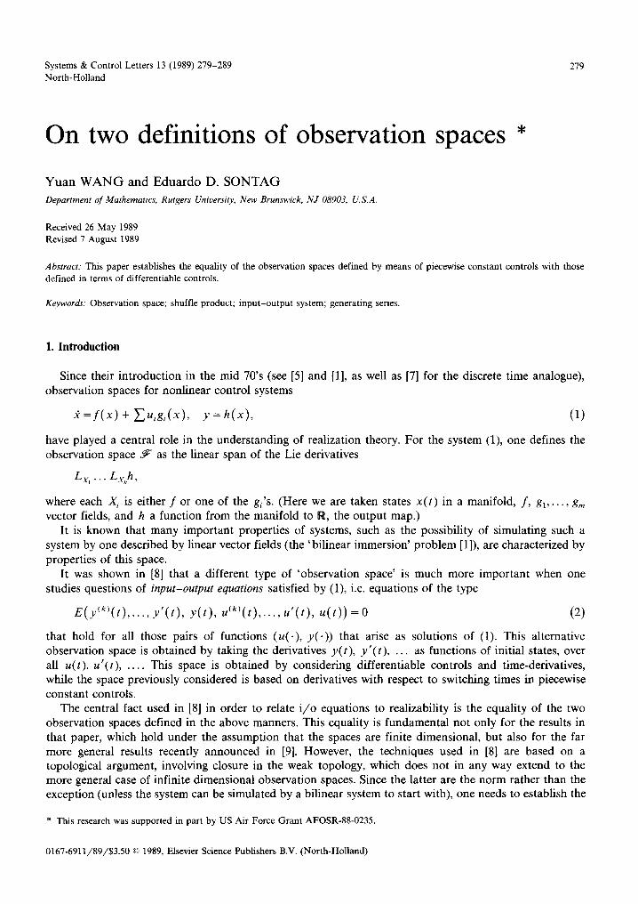
Let m be a fixed integer and I = {0, 1 . . . . . m }. For any integer k > 1, we define I k to be the set of all sequences ( i l i 2 . . . i k ) , where i s ~ I , l < s < k . For k = 0 , we use I ° to denote the set whose only e lement is the emp ty sequence q~. Let

I * = U ~ . (3) k>_O

Then I * is a free mono id with the composi t ion rule:

( i l i2 " ' " i k ) ( J l J2 " ' " J t ) = ( i l i 2 " ' " ik Jl J2 " ' " J l ) .

If t ~ I t, then we say that the length of t, denoted by l t I, is l. Consider now the ' a lphabe t ' set P = { % , 771 . . . . . ~ ) and P * , the free mono id genera ted by P, where

the neutral e lement of P * is the emp ty word, denoted by 1, and the p roduc t is concatenat ion. Let p k = ( ~li, ~1i2 " " " ~1~ : 1 < i s < m , 1 < s < k } for each k > 0. We define ~ to be the R-a lgebra generated by P *, i.e., the set of all polynomials in the variables ~/~'s. A p o w e r ser ies in the n o n c o m m u t a t i v e var iab les % , */1 . . . . . ~/~ is a formal power series

oc

c = ( c , ~ ) + E E (c , 7/,)7/,, (4) k = l ~ I k

where 7/, = ~, 7/i 2 • • • 7/i, if t = i~ i2 • • • it, and (c, ,/,) ~ R. No te that c is a po lynomia l if only finitely m a n y (c, 7/,)'s are non-zero. A power series is nothing more than a m a p p i n g f rom I * to R; as we shall see later, however, the algebraic structures suggested by the series fo rmal i sm are very impor tan t . We use S~ to denote the set of all power series.

For c, d ~ d P and 7 ~ R, yc + d is defined as the following:

( re + d, 7,) = v(c, 7,) + (d , 7,).

Thus, 6 p forms a vector space over R. We shall say that the power series c is c o n v e r g e n t if

I( c, */,) I ~< K M k k ! for each t ~ I k, and each k > 0, (5)

where K and M are some constants. Let T be a fixed value of t ime and let q / r be the set of all essentially b o u n d e d funct ions u : [0, T] ---, R "

endowed with the L 1 norm. We write II u II oo for max{ II u~ II ~: 1 < i < m} if u i is the i-th c o m p o n e n t of u, and [I ui II o~ is the essential supernorm of u v For each u ~ ~ r and t ~ I t, we define inductively the functions V, = V,[u] ~ ~[0 , T] by

Z 0 = l and V, .... i , + , [ u ] ( t ) = f o t U i , ( s ) V ~ . . . . , , + , ( s ) d s , (6)

where u~ is the i-th coordinate of u ( t ) for i = 1, 2 . . . . . m and Uo(t ) - 1. I t can be proved that each m a p

UT--" ~ [ 0 , T ] , u - V,[u]

is cont inuous with respect to L ~ n o r m in q/r , ~0 n o r m in ~'[0, T].

Y. Wang, E.D. Sontag / Observation spaces 281

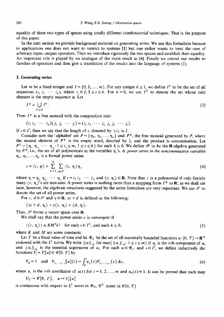
Suppose c is convergent and let K and M be as in (5). Then for any

T< (Mm + M) -1, (7)

the series of functions

E[u](t) = ~_,(c, n , ) V , [ u l ( t ) (8)

is uni formly and absolutely convergent for all t ~ [0, T] and all those u ~ °//r such that l[ u l[ ~ < 1 (cf. [3]). In fact, (8) is absolutely and uni formly convergent for all t ~ [0, T] provided T l[ u [I o~ < (Mm + M ) - k For each nonnegat ive T, let

Y/r = {u~q l r : I]ullo~ < 1 ) . (9)

We say that T is admissible for c if T satisfies (7). Since each opera to r u ~ V~[u] is continuous, it follows that F~: Y/r ~ • 0 , T] is cont inuous if T is admissible for c. We call F C an input-output m a p defined on y/r- Thus every convergent power series defines an i / o map. On the other hand, the power series c is uniquely determined by F c in the following sense:

L e m m a 2.1. Suppose that c and d are two convergent power series. I f F~ = F a on y/r for any T> O, then c = d .

Proof . It is enough to show that if c is convergent and F~ = 0 on Y/r for some small T, then c = 0. Consider piecewise constant controls in Y/r, and use the nota t ion

u = tl)( 2, t 2 ) . . . 0 ,k, tk)

to denote the piecewise constant control whose value is/~i in the t ime interval

(j o J, j =0

where

~ j = ( ~ l j , ~ z j . . . . . ~mj) ~ R ' ~ , ]~ij l < 1 , l<_ j<k , l<_i<_m,

and to = 0. By assumption, for any I~i, ti, such that ~2ti < T, F c[(#1 , ta)(~2, t z ) . . . ( t~k , t ~ ) ] ( t ) = 0, where t = F~ti.

Take y = F~[u] as a funct ion of lal . . . . . /~k and q , - . . , tk- Then

~k t=0+ a~ ~=0 3tl ~ 3 t k Obt,tj, --~)#id,~ y = 0 (10)

for all i 1 . . . . . i~, Ja . . . . . j'~, where the evaluat ion at t + means that we evaluate at t~- . . . . . t [ . We claim that, for i I . . . . . i~, Jl . . . . . j~ given such that j~ ~jq if r 4: q,

0k ,=o+ ,=0 ~t I - - - at k ~/z~d, 3/zid~ y = (c , ~/t~ " ' " *h,), (11)

where

{i~ i f k - ( p - 1 ) = j r , lp= 0 i f k - ( p - a ) c~( j I . . . . . j~).

282 Y. Wang , E .D. S o n t a g / Observa t ion spaces

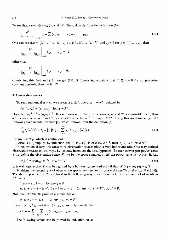
To see this, write y( t ) = Z(c , ~,)V,(t). Then, directly from the definition (6),

~k t=0 + 3t 1 -- ~t k y = ~ (c, 7h, "'" rllk)l~t,k "'" txl, l.

One can see that if ((il, Jl) . . . . . (i~, L) ) c_ ((ll, k) . . . . . (lk, /)} and lp = 0 for p ~ {Jl . . . . . L ) then

~s ~=0 " - / ~ / , k " " " /~l~1 = 1 ;

3Fid, 31XisL

otherwise,

~s /~=0 ~ i l J l - ~l~i~j ~ ~ l l k " " " ~ l k l = O.

Combining this fact and (12), we get (11). It follows immediately that if F~[u] = 0 constant controls, then c = O. []

(12)

for all piecewise

3 . O b s e r v a t i o n s p a c e s

To each monomial a = ~/,, we associate a shift operator c ~ a - 1 defined by

(a - l c , ~/,) = (c, a~/,) for ~, • P * .

Note that a~let( 1 = (ala2)-lc. It was shown in [8] that if c is convergent and T is admissible for c, than a - 1 is also convergent and T is also admissible for a - 1 for any a • P *. Using this notation, we get the following fundamental formula [2], which follows from the definition (6):

d F c I u l ( t ) = F ~ o , c [ u ] ( t ) + ~ u j ( t )Fn; ,c[ul ( t ) (13) j = l

for any u • UT which is continuous. Formula (13) implies, by induction, that if u • zcr T is of class cgk-l, then Fc[u ] is of class cgk. In realization theory, the concept of observation spaces plays a very important role. One may defined

observation spaces in two ways. Let us now introduce the first approach. To each convergent power series c, we define the observation space ~-1 to be the space spanned by all the power series a - l c over R, i.e.,

~ , ( c ) = s p a n . ( a -~c : a • P* }. (14)

It is well known that F C can be realized by a bilinear system and only if dim ~'1(c) < 0o; see e.g. [1]. To define the second type of observation spaces, we need to introduce the shuffle product on ~ (cf. [6]).

The shuffle product on ~ is defined in the following way. First, inductively on the length of of words in P * , we let

l w z = z w l = z for a n y z • P ;

w z l l l w ' z ' = ( w l l l w ' z ' ) z + ( w z W w ) z ' f o r a n y w , w' • P * , z, z" • P .

Note that the shuffle product is commutative:

w l W w 2 = w 2 W w a f o r a n y w ~ , w 2 • P * .

If c = E(c, ~ ) ~ and d = Z (d , ~,)~, are polynomials, then

cwd,=E Z n IKl+l~l~n

The following lemma can be proved by induction on n:

E Wang, E.D. Sontag / Observation spaces 283

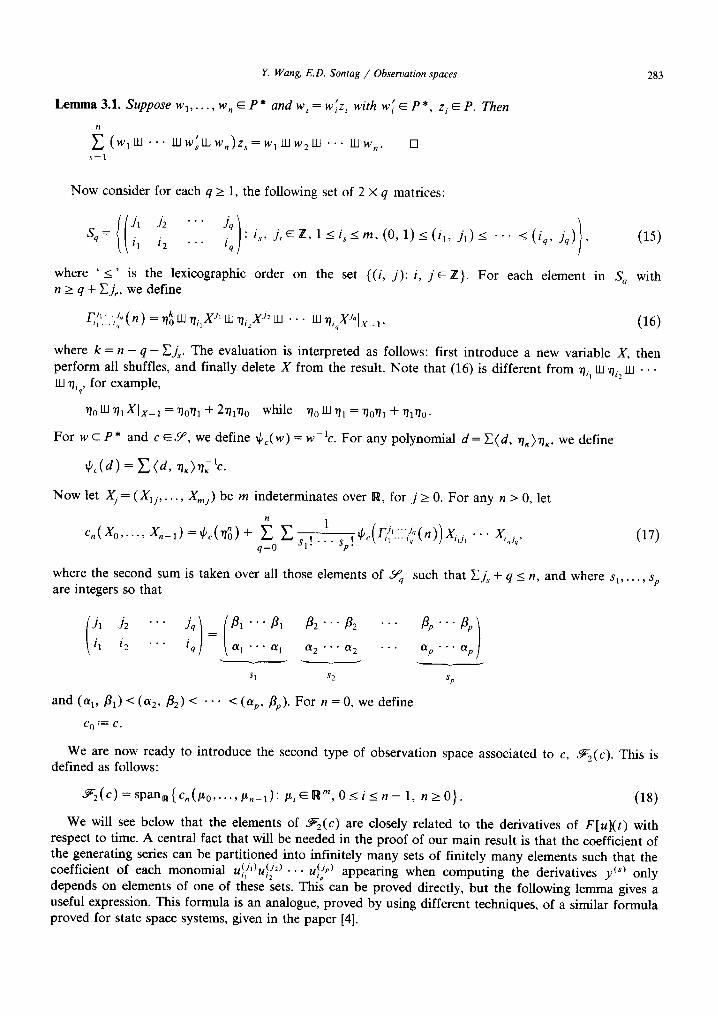
t I Lemma 3.1. Suppose w 1 . . . . , w~ ~ P * and w, = w iz i with w i ~ P * , z~ ~ P. Then

(Wl, , , . . . u:w.. [] s = l

Now consider for each q > 1, the following set of 2 × q matrices:

,) Sq= i, i 2 " " iq : is, J ~ Z ' l < i ' < m ' ( 0 ' l ) < ( i l ' J ' ) < "'" < ( i q , L ,

where ' < ' is the lexicographic order on the set {(i, j ) : i, j E Z } . For each element in n > q + Eft , we define

1~ j',~ . .." q ,( n ,~ = ~ k III 1~il X j l l.l] ~ i 2 X j 2 III • • • I11 ~ i q X J q [ x = 1 ,

(15)

Sq with

(16)

where k = n - q - Ejs. The evaluation is interpreted as follows: first introduce a new variable X, then perform all shuffles, and finally delete X from the result. Note that (16) is different from 7b, w ~/s~ W • • • W ~bq, for example,

'OolllrhXlx=l='OO'ql+2'Oa'Oo while 'OoW~='Oorh+rhr to .

For w ~ P * and c ~ 6 a, we define ~Pc(W) = w--ac. For any polynomial d = E ( d , 7/~)~/,, we define

c(d) = E ( d ,

Now let Xj = (X1j . . . . , Xmj) be m indeterminates over R, for j > 0. For any n > 0, let

n ~ o 1 tPc (F /k ; ; . i Jqq(n ) )X id , . . XiqJq ' c . ( X o . . . . . x . _ , ) = 4 . c ( n o ) + : E s l ! - s, ! (17)

where the second sum is taken over all those elements of 5aq such that EJs + q < n, and where s I . . . . . sp are integers so that

,q):(:: i 1 i 2 " ' " i q ot 1 ol 2 . . . o~ 2 . . .

v

S1 S 2

and (al , B1) < (a2,/32) < " ' " < (ap, tip). For n = 0, we define

C O :=- C .

Otp

Sp

We are now ready to introduce the second type of observation space associated to c, o~2(c ). This is defined as follows:

o ~ 2 ( c ) = s p a n n ( c , ( # o . . . . . # ,_1)" # i ~ n m , o < i < n - 1 , n > O } . (18)

We will see below that the elements of ~-2(c) are closely related to the derivatives of F[u]( t ) with respect to time. A central fact that will be needed in the proof of our main result is that the coefficient of the generating series can be partit ioned into infinitely many sets of finitely many elements such that the coefficient of each monomial uO,)u ( j 2 ) . . . u(Jp ) appearing when computing the derivatives y(S) only "'i l ~'i 2 tp

depends on elements of one of these sets. This can be proved directly, but the following lemma gives a useful expression. This formula is an analogue, proved by using different techniques, of a similar formula proved for state space systems, given in the paper [4].

284 E Wan~ E.D. Sontag / Observation spaces

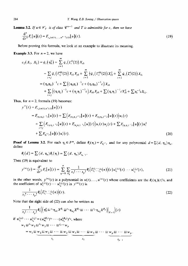
Lemma 3.2. I f u ~ ~/'T is of class c~,-a and T is admissible for c, then we have

d" d t ;F~[u]( t ) = F~.(,(,) ...... . - , ( ,))[u](t) . (19)

Before proving this formula, we look at an example to illustrate its meaning.

E x a m p l e 3.3. For n = 2, we have

c2(X, , X2) =+c(~2) + ~ ~kc(~°(2))Xm i=1

m m

1 o o 2 + Y'- q~c(F~°°(2)) X,o~o + E 7~b¢(F,/ (2))X, o + Y" ~bc(F~l(2))X,~ i<j i=l i=l

= ( ' r / 0 ~ 0 ) - l c q - E ( ( T ~ 0 ' O / ) - I c q - ( ' O l g / 0 ) - l c ) g i 0

-~ E ( ( ~ i ~ j ) - l c - ~ - ( ~ j ~ i ) - l c ) X i o S j o - ~ - E ( ~ i ~ i ) - l c S i 2 o -~ E ~ t l c X i l . i <j

Thus, for n = 2, formula (19) becomes:

y " ( t ) = Fc:(u( t ) ,u , ( t ) )[u]( t )

= F ~ , o . 0 r l ~ [ u ] ( t ) + E(F~,o.y~c[U](t)+ F~,,,o)-'~[u](t))u,(t) + E (F~,nj ) ,~[u]( t ) + F % ~ , ) , ~ [ u ] ( t ) ) u i ( t ) u j ( t ) + ~-"F~,n,),~[u](t)u2i

i < j

+ Y ' .Fn 'c [u] ( t )u ; ( t ) . (20)

Proof of Lemma 3.2. For each ~, ~ P*, define 0~(~/,)= FnT, ~ and for any polynomial d = Y.(d, 7/~)~/~, define

O~(d) = E ( d , ~/~)O~(~,) = Y~, (d, 7/~)Fn:a ~.

Then (19) is equivalent to

d" ~ o ~ l Oc(FiJ~":Te(n)) ( t )u} /° ( t ) ' "uU° ' ( t ) ' (21) y ( n ) ( t ) = - ~ F c [ u ] ( t ) = = Sl ! . - . Sp! 'q "

in the other words, y(")(t) is a polynomial in u(t) . . . . . u(")(t) whose coefficients are the 0~(~,)(t)'s, and the coefficient of u}J')(t) .. (J~) • Uiq ( t ) in y(")(t) is

1_ O ( r J ' J q ( n ) ) ( t ) . ( 2 2 ) Sl! " Sp! c \ q . . . ,q

Note that the right side of (22) can also be written as

_ k s~ B~ ~2 S B z sl! • Sp!

if u}/') • • • u!J~ ) = (u(&)V, • • • (u(&)V, where

WI lIISlw2111S2w3111 . . . IIISp-lWp

= Wl lll W2111W2111 . . . III w2 Ill W3111 . . . III w3 ELl . . . Ill Wp lll . . . Ill W p .

S1 $2 Sp _ 1

Y. Wang, E. D. Sontag / Observation spaces 285

We now use induction to prove the lemma. From (13) we see that the conclusion is true for n = 1. Suppose the conclusion is true for n - 1. Consider the coefficient of ui,‘l’ * * . u,(‘q) in y’“‘. By

inducation from formula (13) it can be seen that Cj, + q I n. First we assume that kj, + q < n. Let k = n - E j, - q. Suppose

&I) . . . ,W = ‘I

,u ( ugv)s’ . . . ( uhlp)y))3p,

where (q, &) < . . . -e (up, j?,). Further, we assume that & = 0 for r I 1. Let

where

and ~,=s;! . . . sit! if

and

I s,! . . . ($1 l)! . . . g e(wJJ(t) if r I I,

i s,! . . . (,’ I)! . . . q e(wJ(t) if r> 1.

Let

v&> =91(t) + l , e,(q!::$(n - l))zp(r) . * * zqql). s,! . . . sp.

By induction assumption, the coefficient of u,(,) . . . ~1’:’ in y’“’ (t) is the same as in r;(t). Thus, this coefficient is 8,(w)(t), where

+5 ,...(,,‘1,!...,,!~:~“~~,~... WS,-‘1),~XB,II177a,XPr-1W ... r=l+l S1.

Ill sp QXP”

(23)

286

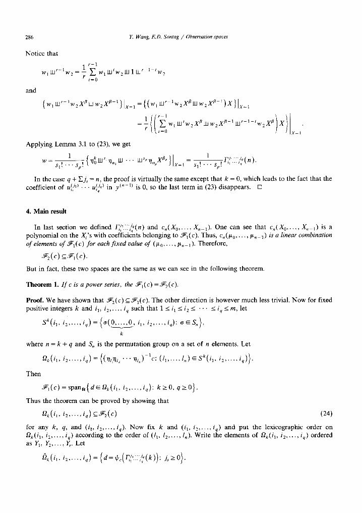
Notice that

1 W 1 l l l r - l w 2 = --

r

and

Y. Wang, E.D. Sontag / Observation spaces

r - 1 E W lJJtw2 ]111 JJ-jr-l-tw 2 t=0

(wi w2s 1)1x=1 = ((w, I]lr-lw2S~ll[ W2 gfl-1 ) g)lg |

1{( r-1 ) X=I" : r

Applying L e m m a 3.1 to (23), we get

W sl! • so!

1

Sl! . - - C ' : : <

In the case q + EJs = n, the p roof is virtually the same except that k = 0, which leads to the fact that the coefficient of u~{ ') . . . u (iq) in y (n - l ) is 0, so the last te rm in (23) disappears . [] iq

4. Main result

In last section we defined /Ta.ii/J)(n) and c , ( X o . . . . . X n _ l ) . One can see that % ( X o . . . . . X , _ 1 ) is a • t . . q .

polynomia l on the Xi's with coefficients belonging to o~-1(c ). Thus, %(1% . . . . . /~,-1) is a linear combination of elements of ~ 1 ( c) for each f i x e d value of (t~ 0 . . . . . t x. - a ). There fore,

~:2(c) _c ~-1(c ) .

But in fact, these two spaces are the same as we can see in the following theorem•

The o rem 1. I f c is a power series, the ~ 1 ( c ) = ~ 2 ( c ) .

Proof . We have shown that ~-2(c) ___ ~1(c ) . The other direction is however much less trivial. N o w for fixed posit ive integers k and i a, i 2 , . . . , iq such that 1 < i I < i 2 < • • • <_ iq <_ m, let

Sk ( i l , i 2 . . . . . iq) = { a ( 0 . . . . . 0 , il, i 2 . . . . . iq): o ~ S n ) ,

k

where n = k + q and S, is the pe rmuta t ion group on a set of n elements• Let

~2k(il, i 2 . . . . . iq) = {(7//1~//2.-. ~ / / . ) - lc : ( l 1 . . . . . ln) ~ s k ( i l , i 2 . . . . . i q ) ) .

Then

o ~ ] ( c ) = s p a n n ( d ~ 2 k ( i 1, i 2 . . . . . i q ) : k > 0 , q > 0 ) .

Thus the theorem can be proved by showing that

~2k( i 1, i 2 . . . . . iq) __.~2(C) (24)

for any k, q, and (il , i 2 . . . . . iq ) . N o w fix k and (il , i 2 . . . . . i q ) and put the lexicographic order on ~ k ( i l , i 2 . . . . . iq ) according to the order of (l a, l 2 . . . . . l , ) . Wri te the e lements of ~2k(i a, i 2 . . . . . iq ) ordered as Y1, II2 . . . . . Yr- Let

= Jl "'" Jq • O \ . ~ k ( i l , i 2 , . . . , iq) ( d = l ~ c ( F i l . . . i q ( k ) ) js > I

Y. Wang, E.D. Sontag / Observation spaces 2 8 7

Then we have lak(i 1, i: . . . . . iv) _c.~2(c ). Put the lexicographic order on ~2k(il, i 2 . . . . . i q ) according to the order of (E j , , Jl . . . . . jq). Notice that for each element di ~ ~2k(il, iz . . . . . iq) , there exist some posit ive integers aii such that

d i = ~ a i j ~ . j=l

Let A be the matr ix of r colunms and infinitely m a n y rows whose (i, j ) - t h ent ry is aij , i.e., A = ( a o ) . We claim that A is of full co lumn rank in the sense that there is no nonzero vector v ~ R" such that

Av = 0. Suppose there is some v :~ 0 such that Av = 0. Const ruc t a po lynomia l e in the following way:

(e , r/h " "" vi i , )= 0

if (l 1 . . . . . lt) ~ Sk ( il, i2 . . . . . i q) and

(e , rll, ' ' ' ~ll,) = vi

if (ll . . . . . l,) E Sk ( i> i 2 . . . . . iq) and (~lt, " ' " ~l,) - l c corresponds to the i-th e lement of ~2k(il, i 2 . . . . . iq). By the definit ions of A and d, we know that

e,(/~ 0 . . . . . /x.,) = 0 for any n.

Therefore,

d" dt" Fe[u](O) = Fa"(~° ..... ~,, ,}[u](0) = 0

for any n and any analytical control u, which implies that Fe[u ] = 0 for any analytical controls. Since analytical controls are dense in ~e" r (under the L x topology), it follows that F e - 0. By L e m m a 2.1, e = 0. Thus, v = 0, a contradic t ion to the assumption. Hence, A is of full co lumn rank.

N o w let ~ , be the subspace of R r spanned by the first s row vectors of A. Then

s e l c ,2c . . . . . . .

Since .~e c R r for any s, there exists some s o > 0 such that ~¢s =~¢s0 for every s > s 0. Let A 1 be the s o × r submatr ix of A consisting the first s o rows of A. Then A = TAt for some matr ix T. Therefore rank A1 = r. By the construct ion of Aa, we know that

111 dl )

Y2 d : A 1 • =

Yr d!so

F r o m the facts that d~ ~.~-2(c) and A 1 is of full co lumn rank, we get the conclusion that Y, ~o~2(c ) for each i, therefore, (24) holds.

Since k, q and (i 1, i 2 . . . . . iq) were arbi trary, we get the desired conclusion Owl(e ) =o~2(c ). []

5. Families of series and systems

In this section we consider families of power series. Let A be a index set. We say that c is a family of power series (parameter ized by X ~ A) if c := { c x : X ~ A }, where c a is a power series for each fixed 2,. A family c can also be viewed as a power series with coefficient belonging to the ring of functions f rom A to R, i.e,

e = I2 ( c , n ,>n, ,

where (e, n,) : A ~ N, (e , rh)()~) ~ (c x, ~/,).

288 Y. Wang, E.D. Sontag / Observation spaces

Let ® be the set of all families of power series. For c, d ~ ® and 7 ~ R, yc + d is defined to be the family of power series ( ' / c a + d x : k ~ A }. Thus ® forms a vector space over R.

We say that c is a convergent family if each m e m b e r of the family is convergent . For any monomia l a ~ P*, a - lc is def ined to be the family { a - l c ~' : ~k ~ A ). For any n > O, c . ( X o . . . . . X . _ I ) is defined to be the family

{ c. (x0 ..... xo_l): X A},

where ~ = ( X n . . . . . Xi.,) are m indeterminates over R, i > 0. Apply ing 3.2, we have that

d" dt----gFc~[u](t) = Fc~(u(o . . . . . . . - , ( t ) ) [u ] ( t ) , (25)

for each k. As in the case of single power series, we associate to c two types of observa t ion spaces in the following

way:

~ 1 ( c ) := spann { a - a c : a ~ P * },

~ 2 ( c ) := spann{en( /z0 . . . . . /.tn_l): t~i~Rm, O<_i<_n-1, n>__O).

Note that ~ l ( e ) (respectively, ~ 2 ( e ) ) is formal ly analogous to ~ 1 ( c ) (respectively, ~ 2 ( c ) ) studied before. Using c and d instead of c and d in the p roof of Theo rem 1, we get the following result:

Theorem 2. I f c is a family of power series, then ~ a ( e ) = 52(¢). []

N o w consider a state space system

Yc = go(x) + Y~.uig,(x), y = h ( x ) , (26)

where x( t ) ~ X, a ~ " manifold, go, gl . . . . . g,, are cg~ vector fields, and h a cg~ funct ion f rom X to R. One type of observat ion space associated with (26) is

F 1 := span a (Lg , , . . . Lg,kh: k > 0) .

For/~0 . . . . . /~k-1 given, we let, for each x ~ X,

dk ,=o y~o ' " ~ ' - ' ( x ) : = dt---- ~ yx(t) ,

where y~(t) is the output corresponding to initial state x and any c~¢ input u such that u(J)(0) = /z j for O < j < k - 1 .

We associate to (26) a second type of observat ion space, as follows:

F 2 := span n ( y"~ "" "~-~: /z i ~ R " , k > 0}.

By a fundamenta l formula due to Fliess (see [3]), the i n p u t - o u t p u t m a p of (26) can be writ ten as

y ( t ) =F~[u]( t ) ,

where the family c is def ined by (c, ~/,~ - - - 7/,~) = Lg,, . . . Lg, h, or, equivalently, for the output corre- sponding to the initial state x,

yx(t) = Fc~[u] ( t ) ,

where (c ~, */i~ " ' " */ik) = Lg,~ . . . L g q h ( x ) . Thus,

gg,k ' ' ' gg i lh = (C , ~i] "°° ]]i k ) = ( ( ~ i 1 " * " ~ ik ) - l c ' ¢~)'

Y. Wang, E.D. Sontag / Observation spaces

and , therefore,

F, = {~d , qS): d ~ ~ t ( c ) } .

By (25), we k n o w tha t y~O ... ~, , = F,.Z~, ...... , , ,)[u](0) = ~c{(#o . . . . . /~k-1), ~ ) - Hence ,

F 2 = { c a , q~>: d ~ ~ 2 ( c ) ) .

So the fo l lowing c o n c l u s i o n follows i m m e d i a t e l y f rom T h e o r e m 2:

Corol la ry 5.1. For the state space system (26), F 1 = F 2. []

289

References

[1] M. Fliess and I. Kupka, A finiteness criterion for nonlinear input-output differential systems, SlAM .L Control Optim. 21 (1983) 721-728.

[2] M. Fliess and C. Reutenauer, Une application de l'algebra differenti611e aux systSmes reguliers (ou bilin~aires), in: A. Bensoussan and J.L. Lions, Eds., Analysis and Optimization of Systems, Lect. Notes. Control Informat. Sci. No. 44 (Springer-Verlag, Berlin-New York, 1982) 99-107.

[3] A. Isidori, Nonlinear Control Systems: An Introduction (Springer, Berlin-New York, 1985). [4] F. Lamnabhi-Lagarrigue and P.E. Crouch, A formula for iterated derivatives along trajectories of nonlinear systems, Systems

Control Lett. 11 (1988) 1-7. [5] J.T. Lo, Global bilinearization of systems with controls appearing linearly, SlAM J. Control 13 (1975) 879-885. [6] M. Lothaire, Combinatorics on words, in: G.C. Rota, Ed., Encyclopedia of Mathematics and its Applications, Vol. 2 (Addison-Wes-

ley, Reading, MA, 1983). [7] E.D. Sontag, Polynomial Response Maps (Springer, Berlin-New York, 1979). [8] E.D. Sontag, Bilinear realizability is equivalent to existence of a singular affine differential i /o equation, Systems Control Lett. 11

(1988) 181-187. [9] Y. Wang and E.D. Sontag, A new result on the relation between differential-algebraic equation and state space realizations, in:

Proceedings of Conference on Information Sciences and Systems (Johns Hopkins University, March 1989) 143-147.