ON THE VISUALIZATION OF DOMAIN RESULTSIN TWO-DIMENSIONAL BOUNDARY ELEMENT ANALYSIS

André Maués Brabo PereiraMarcos Aurélio Marques NoronhaDepto. de Engenharia de Estruturas e Fundações – Universidade de São PauloEscola Politécnica – 05508-900 – São Paulo - SP, Brazilmaues.pereira , marcos.noronha@poli.usp.brRemo Magalhães de SouzaDepto. de Construção Civil – Universidade Federal do ParáCentro Tecnológico – 66075-970 – Belém - Pa, Brazilremo@ufpa.br

Abstract. Most postprocessors for BE analysis uses an auxiliary domain mesh to displaydomain results, working against the profitable modeling process of pure BEMs. Recently, thetwo first authors of this paper presented a new visualization algorithm based on the directand automatic identification of isocurves. This algorithm does not require any domaindiscretization, preserving the basic properties of the BEM. One of the critical aspects of thevisualization of domain results in BE analysis is the computational effort required for theevaluation of results in interior points. For the conventional formulation of the BEM, this lastprocedure demands a relatively high computational effort. On the other hand, the hybridformulation of the BEM represents a powerful alternative to improve the performance ofthose evaluations, since the domain results are obtained without evaluation of integrals. Thispaper discusses some aspects related to the visualization of domain results in BE analysis. Inaddition, it also compares the performance of the conventional and hybrid formulations of theBEM using different visualization procedures. Some examples show the results of the presentstudy. Finally, the paper discusses on new applications of the visualization algorithms,specially for nonlinear analyses with BEM.

Keywords: Boundary Element Methods, Scientific Visualization, Contour Plot.

1. INTRODUCTION

In the recent years, due to the increasing number of research and technological advances,Computer Graphics has been expanding rapidly into other fields and areas of knowledge(Foley, 1997) (Farin, 2002). The application of Computer Graphics in engineering and inother scientific and technological areas has been fundamental to the development of newresearches on the visualization of scientific data. Nowadays, the computational simulation ofcontinuum mechanics problems demands an extensive use of graphical applications.

Among other numerical methods, the Finite Element Method (FEM) and the BoundaryElement Method (BEM) are the most significant techniques for continuum mechanicsproblems. One of the main advantages of the BEM over the FEM is the low effort of itsmodeling process. Pure BEMs should represent models only with boundary discretization.However, to accomplish the visualization of domain results, most BEM implementations usesan auxiliary domain discretization. This is a natural approach for the FEM, which uses a meshover the domain to represent the model. However, this procedure is inadequate for BEMs,since no domain discretization should be necessary. In addition, this procedure can neglectcritical results that occur in regions with high gradients, then its efficiency is questionable.

The authors have not find in the literature any specific technique for the visualization inBE analysis. Hence, they developed a new procedure without domain discretization based onthe direct and automatic identification of isocurves and isobands. Basically, it consists in acombination of iterative and predictive procedures and spline adjustment techniques.

This paper also discusses some aspects related to the visualization of domain results inBE analysis, comparing the conventional algorithms with auxiliary domain discretization tothe new visualization algorithm proposed. It also compares the performance of theconventional BEM to the hybrid formulation of the BEM, an alternative technique which doesnot require integral calculations to obtain results at interior points.

2. BOUNDARY ELEMENT FORMULATIONS

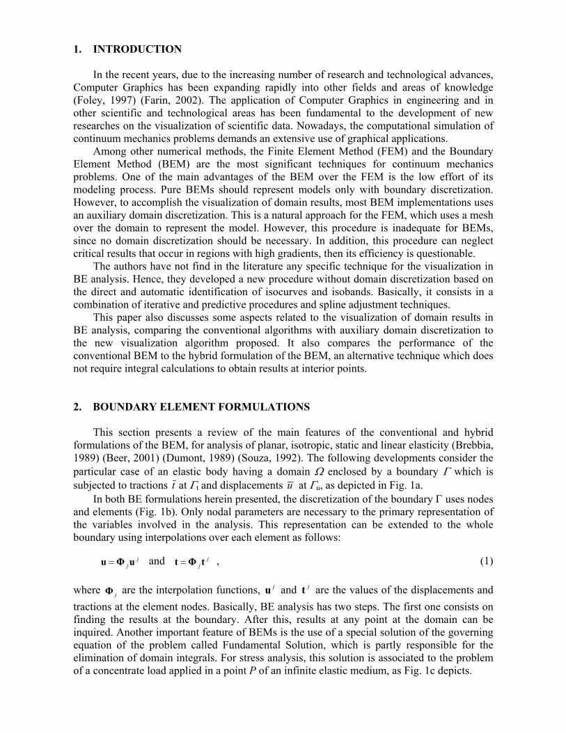
This section presents a review of the main features of the conventional and hybridformulations of the BEM, for analysis of planar, isotropic, static and linear elasticity (Brebbia,1989) (Beer, 2001) (Dumont, 1989) (Souza, 1992). The following developments consider theparticular case of an elastic body having a domain Ω enclosed by a boundary Γ which issubjected to tractions t at Γt and displacements u at Γu, as depicted in Fig. 1a.

In both BE formulations herein presented, the discretization of the boundary Γ uses nodesand elements (Fig. 1b). Only nodal parameters are necessary to the primary representation ofthe variables involved in the analysis. This representation can be extended to the wholeboundary using interpolations over each element as follows:

jjuΦu = and j

j tΦt = , (1)

where jΦ are the interpolation functions, ju and jt are the values of the displacements andtractions at the element nodes. Basically, BE analysis has two steps. The first one consists onfinding the results at the boundary. After this, results at any point at the domain can beinquired. Another important feature of BEMs is the use of a special solution of the governingequation of the problem called Fundamental Solution, which is partly responsible for theelimination of domain integrals. For stress analysis, this solution is associated to the problemof a concentrate load applied in a point P of an infinite elastic medium, as Fig. 1c depicts.

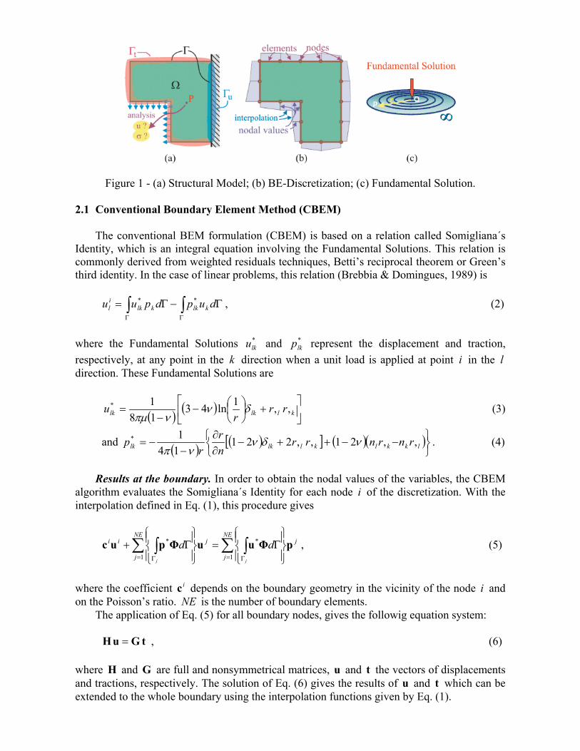
Figure 1 - (a) Structural Model; (b) BE-Discretization; (c) Fundamental Solution.

2.1 Conventional Boundary Element Method (CBEM)

The conventional BEM formulation (CBEM) is based on a relation called Somigliana´sIdentity, which is an integral equation involving the Fundamental Solutions. This relation iscommonly derived from weighted residuals techniques, Betti’s reciprocal theorem or Green’sthird identity. In the case of linear problems, this relation (Brebbia & Domingues, 1989) is

∫∫ΓΓ

Γ−Γ= dupdpuu klkklkil

** , (2)

where the Fundamental Solutions *lku and *

lkp represent the displacement and traction,respectively, at any point in the k direction when a unit load is applied at point i in the ldirection. These Fundamental Solutions are

( ) ( )

+

−

−= kllklk rr

ru ,,1ln43

181* δν

νπµ(3)

and ( ) ( )[ ] ( )( )

−−++−∂∂

−−= lkklkllklk rnrnrr

nr

rp ,,21,,221

141* νδννπ

. (4)

Results at the boundary. In order to obtain the nodal values of the variables, the CBEMalgorithm evaluates the Somigliana´s Identity for each node i of the discretization. With theinterpolation defined in Eq. (1), this procedure gives

∑ ∫∑ ∫= Γ= Γ

Γ=

Γ+NE

j

jNE

j

jii

jj

dd1

*

1

* pΦuuΦpuc , (5)

where the coefficient ic depends on the boundary geometry in the vicinity of the node i andon the Poisson’s ratio. NE is the number of boundary elements.

The application of Eq. (5) for all boundary nodes, gives the followig equation system:

tGuH = , (6)

where H and G are full and nonsymmetrical matrices, u and t the vectors of displacementsand tractions, respectively. The solution of Eq. (6) gives the results of u and t which can beextended to the whole boundary using the interpolation functions given by Eq. (1).

Results at internal points. After solving Eq. (6), the displacements for any point in thedomain Ω can be evaluated using the Somigliana´s Identity, Eq. (2). In a similar manner,results for the stress tensor can be obtained at internal points by

∫∫ΓΓ

Γ−Γ= duSdtD kkijkkijijσ , (7)

where

( ) ( )( ) kjikijikjjkikij rrrrrrr

D ,,,2,,,21141

+−+−−

= δδδννπ

(8)

( ) ( ) ( )[ ]+ −++−

∂∂

−= kjiijkjikkijkij rrrrrr

nr

rS ,,,4,,,212

12 2 δδνδννπ

µ

( ) ( )( ) ( ) ijkjkiikjjikkijkji nnnrrnrrnrrn δνδδνν 41,,221,,,,2 −−++−+++ . (9)

Extended results. In order to obtain the isocurves of the stress field in Ω, thevisualization algorithm proposed in this paper requires the stress tensor derivatives. Thesederivatives can be evaluated using the following expression:

∫∫ΓΓ

Γ−Γ= duSdtD kmkijkmkijmij ,,,σ , (10)

where

( ) ( )( ) ( )jikmkijmkjimkmijimkjjmkimikjmkij rrrrrrrrrrrrr

rDr

D ,,,,,,,,,2,,,21141,1

, +++−+−−

+= δδδννπ

(11)

and

( )( ) ( )[ ]

( ) ( ) ( )[ ]( ) ( )[ ] ( ) ( ) . ,,,,221,,,,,,,,2

,,,,,,,,,4,,,21,2

,,,4,,,21,212

,212,

ijmjimkikmkimjjkmkjmi

jikmkijmkjimimjkjmikkmij

kjiijkjikkijmmkijmkij

rrrrnrrrrnrrrrn

rrrrrrrrrrrrr

rrrrrrrr

rSr

S

+−+++++

++−++−

+−++−−

+=

νν

δδνδν

δδνδννπ

µ

η

η

(12)

The evaluation of results in points at the boundary requires calculation of singularintegrals. In addition, calculation for points close to the boundary involves quasi-singularintegrals. Both evaluations require a special integration scheme (Dumont & Noronha, 1998).To avoid those effects, this work considers visualization at regions shifted from the boundary.

2.2 Hybrid Boundary Element Method (HBEM)

The hybrid BEM formulation (HBEM) is based on the Hellinger-Reissner variationalprinciple (Dumont, 1989). The Hellinger-Reissner potential ΠR can be expressed as

∫∫∫ΓΓΩ

Γ+Γ−Ω+=Π−σ

ησσ dutduduDU iijijiijijijc

R**

,**

0 ])([ , (13)

where )( **0 ij

cU σ is the complementary strain energy, and *ijσ is the stress field at the domain,

which is given by a linear combination of fundamental solutions as

**kkijij pD=σ , (14)

where *p is a vector of singular forces.

In a similar manner, the derivatives of the stress field at the domain can be expressed as

*,

*, kmkijmij pD=σ , (15)

where mkijD , is the derivative of the fundamental solution for stresses, Eq. (11).

Results at the boundary. After discretization and application of the principle of stationarypotential energy to the Hellinger-Reissner potential, the problem can be expressed as

=

−p0

dp

0HHF *

T , (16)

where d is the nodal displacement vector, F is a symmetric flexibility matrix, H is the samematrix of the CBEM and p is the vector of nodal forces equivalent to the boundary tractions.

Solving the first equation in the system of Eq. (16) for *p results in

dHFp 1* −= . (17)

Substitution of *p in the second equation of the system Eq. (16) gives

pdK = , (18)where K is a symmetric stiffness matrix, given by HFHK 1T −= , where 1F − is ageneralized inverse of F . For more details, the reader is referred to (Dumont,1989). Solutionof Eq. (18) gives the results of d and p at the discretization nodes.

Results at internal points. After solving Eq. (18) and substitution of results in Eq. (17),the stress and the displacements for any point in the domain Ω should be defined through thenodal forces *p , except on the points of application of these forces. Then, the stress field at Ωand its derivatives can be obtained directly from Eq. (14) and Eq. (15).

Since no integration is necessary, the evaluation of internal results with the HBEMbecomes simpler and faster than any other method. On the other hand, there are also somedrawbacks, as the behavior of the results close to the nodes of the discretization, whichinvariably tends to infinity. Another drawback is the evaluation and inversion of matrix F ,which demand a high computational effort.

3. VISULIZATION TECHNIQUES

The isocurve plot technique (Fig. 2a) is one important tool that analysts commonly use tovisualize data for 2D engineering problems. For a scalar function ( )xf where 2R∈x , anisocurve segment is the set of points x which satisfy ( ) iff =x at the interval [ ix , fx ], where

if is the level or height of the isocurve segment with ix and fx as limiting points (Figure 2b).For a given point of an isocurve the normal and tangent unit vectors are given by

2

2

2

1

T

21

∂∂

+

∂∂

∂∂

∂∂

=xf

xf

xf

xfn and

2

2

2

1

T

12

∂∂

+

∂∂

∂∂

∂∂

=xf

xf

xf-

xft . (19)

Figure 2 - (a) Isocurve plot; (b) isocurve definitions; (c) particular case of enclosed isocurves.

In these plots, it is useful to use a color palette to display the single connected regionsbetween the isocurves, which are called isobands. The isoband color gives a clear indicationof the function level over the model domain. Before presenting the proposed algorithm, thissection discusses on the characteristics of the most popular isocurve plot techniques.

3.1 Scan line algorithm

The scan line algorithm is one of the simplest techniques to display isocurve plots. Thealgorithm consists on the evaluation of the function for each pixel included at the modeldomain. Therefore, it depends on the scale of the model and on the resolution of the rasterdisplay used. The plot is guided by a scan line which moves from the top to the bottom of themodel. For each scan line location, the algorithm performs intersection tests to find the initialand final points of the segments over the scan line (Fig. 3a). The next step consist in thesequential evaluation of the function at the center of each pixel on the segment considered.According to the function value, the pixel is displayed using the color palette available (Fig.3b). Figure 3c displays an isocurve plot for the horizontal stress component using the scanline algorithm for a simulation with the CBEM. For this plot, evaluations of the requiredfunction at 120.000 points were necessary. Clearly, this is not adequate for practical uses andshould be avoided since it demands a high computational effort. A slight improvement of theperformance of the scan line algorithm can be achieved applying a single evaluation to arectangular group of pixels. Due to the loss of accuracy, the cost-benefit of this last approachmakes it inadequate for practical purposes.

Figure 3 - (a) Scan line algorithm; (b) evaluation at pixels; (c) final plot with 120.000 pixels.

3.2 Interpolation over an auxiliary domain discretization

A better approach for the isocurve plot consists in a technique based on interpolation overan auxiliary domain discretization. Probably, this is the most common procedure used bycommercially available programs. There are different versions of this algorithm. The simplestone is similar to the scan line algorithm. It requires a simple discretization of the modeldomain and the set of results at each node of this discretization. For each unity of thediscretization, results are interpolated from the nodes using similar tecniques of the FEMinterpolation (Fig. 4a). This approach works well for the FEM, since a domain mesh andinterpolation functions are already available. However, it works against the basic properties ofthe BEM, which should use only boundary discretization. In addition, the accuracy of thisprocedure depends on the discretization level used and can display results with insufficientquality, due to the jagged appearance of the isocurves. Another even worse aspect is that itcan ignore critical isocurves in regions with high gradients of the function (Fig. 4b).

For practical purposes, this technique requires at least an adaptive discretization in orderto deal with the regions with high gradients. Therefore, for the BEM the efficiency of thisalternative is questionable, since the task of mesh generation at the domain attains the samecomplexity of the FEM modeling process.

Figure 4 - (a) Domain discretization and interpolation; (b) accuracy problems.

3.3 Proposed Algorithm

In order to overcome the drawbacks of the two previous techniques, the authors of thispaper developed a new algorithm for the isocurve plot in analysis with BEMs. The proposedalgorithm uses the specific features of the BEM in a rational manner, preserving its basiccharacteristics. The central idea is to accomplish the automatic and direct identification of theisocurves. For a smooth representation of isocurves, it adjusts segments of cubic splines(Foley, 1997). To obtain the control points of the splines, the algorithm uses the predictiveand iterative techniques commonly used in non-linear analysis (Crisfield, 1991). In order torestrain the computational effort, the governing parameters of the incremental process (stepsize, convergence criteria) should result in evaluations at a small number of internal points.For the sake of simplicity, the authors suggest a heuristic adjustment of these parameters.

The present implementation deals only with the most frequent case of isocurves emergingfrom the boundary. The case of isocurves enclosed in an isoband will be discussed in futureworks, since it requires an auxiliary algorithm to find an initial point on the isocurve (Fig. 2c).

The first step of the algorithm consists in finding the limiting points at the boundary ofthe model, storing them in a list according to their occurrence (Fig. 5a). For isocurves

representing the displacement field, these points should be obtained using the interpolationfunctions of Eq. (1). On the other hand, isocurves for the stress field need a special treatmentto the hypersingular integrals present in Eqs. (7) and (10). A simple alternative to this is theso-called “traction-recovery” method (Beer, 2001).

Starting from a initial point ix , the proposed algorithm consists in finding a new pointlying on the isocurve, tracking its path in an incremental manner (Fig. 5b). For this task, thealgorithm combines two different procedures. The first one is a prediction estimate, whichlocates the new point on the tangential direction using a scalar step size t∆ as follows:

txx .tip ∆+= . (20)

An adequate choice for the step size t∆ will be presented later on in this section.For curved paths, point px will drift from the isocurve. The second procedure of the

algorithm consists in using iterative techniques to find the new point nx on the isocurve. Mostiterative techniques uses the Newton-Raphson method (N-R) in conjunction with constraintconditions that define the returning direction for the point px . In the last two decades, the arc-length methods (Crisfield, 1991) have been successfully used for non-linear applications.

An alternative approach to the arc-length methods is the “normal flow” method, which isrelated to the proposed algorithm (Ragon, 2002). This method is based on the “Davidenkoflow” concept, which represents the set of perturbations to a path (Fig. 5b). For the presentapplication, these perturbations are the set of isocurves adjacent to if . The normal flowmethod uses the normal direction to the Davidenko flow as the returning path for the N-Riterations. For the proposed algorithm this is the direction of the unit normal vector defined onEq. (19). Thus, in order to find the new point nx , successive iterations are evaluated by

( )[ ]12

2

2

1

11 . −

−−

∂∂

+

∂∂

−+= j

jijj

xf

xf

ffn

xxx , for ,...2,1=j , (21)

where the first point corresponds to the result of the prediction phase ( pxx =0 ).The new point nx is obtained by recursive evaluations of Eq. (21) until the fulfillment of

a convergence criteria, which should be a simple error norm as

( )i

ij

f

ff

∆

−=

xε , (22)

where if∆ is the isocurves level interval. The present implementation considered 001.0=ε .The choice of the normal direction as the returning path results in a unique minimum normsolution for the N-R iterations. Due to this feature, it is expected that a small number ofiterations (1 or 2) will satisfy Eq. (22).

The algorithm proceeds with new prediction and iterative steps, using point nx of the N-R iterations as the initial point ( ni xx = ), until it finds the final point fx at the boundary.Then, it removes ix and fx from the list of limiting points. If this list is not empty, thealgorithm goes further to the next isocurve.

Figure 5 - (a) Limiting points; (b) predictive and iterative phases.

The present algorithm requires the partial derivatives of ( )xf during the predictive anditerative processes. This additional information allows a suitable approximation of the curvebetween the points ix and nx using cubic splines, since the tangent vectors are promptlyavailable. Normally, just few spline segments will represent the isocurve with good accuracy.

The step size t∆ used for the prediction phase depends on several factors, e.g. theisocurve distribution, the model geometry and the required degree of accuracy. There are amyriad of ways to combine these factors, making the choice of an appropriate step size t∆ arelatively difficult task. The present implementation used a heuristic approach to determinethe step size t∆ . It is a simple attempt to avoid isocurve intersections, setting t∆ as the half ofthe distance between two points adjacent to the initial point (Fig. 6a). These adjacent pointsare either the initial points of other isocurves or the model corners.

For each prediction estimate, in order to limit the deviation from the actual isocurve levelto 20%, the algorithm evaluates a new step size newt∆ as follows:

( ) tfxf

ft

ip

inew ∆

−

∆=∆

2.0 . (23)

To avoid strong deviations, a range is established for the new step size, varying between halfand double of the t∆ value.

If the current values of ( )pf x differs more than 20% from if , the algorithm performs newpredictions using newt∆ , before the iterative phase, until the error norm of Eq.(22) is less than20%. On the other hand, newt∆ will be used only for the prediction phase of the next segmentof the isocurve, thus providing an automatic adjustment for the step size (Fig. 6b).

Figure 6 - Step size: (a) initial determination; (b) automatic adjustment.

4. IMPLEMENTATION

Recently, the authors have been involved in the development of a computational platformfor BEMs. The platform consists in an integrated system with an analysis core and graphicalpre- and postprocessors, using the features and benefits of the object-oriented programming(OOP) with Java (Booch, 1999) (Ammeraal, 1998).

Figure 7 - Class diagram for the postprocessor with the new class IsocurveView.

In other to implement the proposed algorithm, the application of object-oriented analysisand design processes resulted in the inclusion of the new class IsoCurveView in the existingpostprocessing class architecture. Figure 7 displays the class diagram using UML Notation(Booch, 1999). This new class uses cubic splines, Half-edge (HED) data structure (Mäntylä,1988) and several graphical algorithms (intersections, point location) implemented in thepostprocessor. Due to the HED, the implementation allows the automatic identification of theisobands. Additionally, the class IsocurveView is associated to classes CBem and HBem,which represent the conventional and hybrid BEM, respectively, allowing the evaluation ofdisplacements and stresses (and their derivatives) in interior points with both methods.

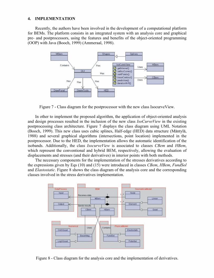
The necessary components for the implementation of the stresses derivatives according tothe expressions given by Eqs (10) and (15) were introduced in classes CBem, HBem, FundSoland Elastostatic. Figure 8 shows the class diagram of the analysis core and the correspondingclasses involved in the stress derivatives implementation.

Figure 8 - Class diagram for the analysis core and the implementation of derivatives.

The sequence of steps of the new visualization algorithm might be represented using aFinite State Machine, a valuable tool in the object-oriented analysis and design. Figure 9displays the state transition diagram which indicates the dynamic behavior of classIsoCurveView using UML Notation (Booch, 1999).

Figure 9 - State transition diagram of class IsoCurveView.

5. NUMERICAL RESULTS AND EXAMPLES

In order to illustrate the different aspects related to the visualization techniques discussedin this article, this section presents results using the proposed algorithm, the intepolation overdomain discretization and the scan line technique.

5.1 Results with the proposed algorithm

This section presents two test examples which demonstrate the proposed algorithmaccuracy and efficiency in analyses with the CBEM. The first example consists in a cantileverbeam with a load applied to its free end. For this analysis, a regular discretization with 48linear elements was used. To avoid quasi-singular integrals, the present implementation usedan auxiliary boundary inside the real boundary. The distance between both is half of theelement size. Figure 10 shows the results for the xxσ stress field using a set of 11 equallyspaced isocurves. This plot required evaluations at 43 interior points, using just one N-Riteration to correct the prediction estimate. The resulting isocurves agree very closely with theanalytical results from the theory of elastic bending of beams.

Figure 10 - Application of the algorithm for the analysis of a cantilever beam.

A comparison between the proposed algorithm and the interpolation over a domaindiscretization has been made using analysis with the FEM. As Figure 11 depicts, the results ofthe proposed algorithm using 43 interior points were more accurate than a mesh using 80finite elements of type Q9, which has 369 interior points. Additionally, in contrast with thedomain discretization, the proposed algorithm resulted in smoothly continuous isocurves.

Figure 11 - Proposed algorithm and the interpolation over a domain discretization.

The second example consists in a L-shape body with stress concentration. The modelrepresentation used a regular discretization with 40 linear elements. Figure 12a presents thealgorithm results. This plot required evaluations at 115 interior points. To correct theprediction estimate, 58 interior points required just one N-R iteration, 54 points required 2iterations, 2 points required 3 iterations and just 1 point required 4 iterations. Figure 12bshows an enlarged view of an area of the isocurve plot to closely inspect the predictive anditerative processes.

Figure 12 - (a) Isocurves for a L-Shape; (b) close view of the incremental process.

The comparison using the interpolation over domain discretization using the FEM isdepicted in Fig. 13. The results with the proposed algorithm using 115 interior points weremore accurate than the plot for a domain discretization with 320 finite elements of type Q9,which has 1281 interior points.

Figure 13 - Comparison for the L-Shape.

5.2 Results with the scan line algorithm for CBEM and HBEM.

As discussed in section 2, evaluation of results in interior points using the HBEM is muchsimpler and faster than the procedure required by the CBEM. This section presents results forthe scan line algorithm applied to both methods, comparing the computing time required onlyfor the visualization. Figure 14 displays results for a simply supported beam represented by48 linear boundary elements.

Figure 14 - Comparisons using scan line for a simply supported beam.

The scan line algorithm was applied considering evaluations at a single pixel (1x1) and ata group of 5x5 pixels as well. Due to the integral calculations, the CBEM required a muchhigher computing time (about a factor of 35) than the HBEM. On the other hand, problemswith jumps and lack of accuracy in regions close to the boundary were more pronounced inthe HBEM. These effects can be reduced with a more refined discretization. Figure 15 showsresults with the HBEM for a mesh with 96 boundary elements. Now the solution behavior ispractically the same of the CBEM, and the computing time for these visualizations was onlytwice that of the previous examples with the HBEM.

Figure 15 - Results using a more refined discretization.

The results of the application of the scan line algorithm to the L-Shape also presented thesame characteristics from the previous example (Fig. 16). Again, the computing time requiredby the CBEM was about 35 times higher than the analysis with the HBEM.

Figure 16 - Comparison for the L-Shape.

It is worth to emphasize that the results presented in this section are not conclusive aboutthe characteristics of the CBEM and the HBEM in visualization of results. The computingtime necessary for the first part of the analysis (solution at the boundary) has also to beconsidered. In addition, an adequate integration scheme for the CBEM has to be used,allowing the visualization of the results at the whole domain.

6. CONCLUSIONS

This article addressed the task of visualization of domain results in analysis with BEMs.In the last two decades, much research has been done on the development and implementationof BEMs. However, the advances in the visualization algorithms were insignificant. After anextensive literature review, the authors have found that the visualization task for BEMspractically uses the same techniques for the FEM. Therefore, they proposed a new algorithmwhich makes a convenient use of the specific BEM properties, as the flexibility of inquiringresults and their derivatives at interior points. Several examples using different visualizationtechniques demonstrate the accuracy and efficiency of the proposed algorithm. In addition,this work also carried out performance tests of two different formulations of the BEM.

The tests with the scan line algorithm show that this technique requires a high number ofevaluations, but its usage is not prohibitive for analysis using the HBEM, since it involves alow cost operation to evaluate results at interior points. However, further investigations arenecessary, considering the computing time required to obtain the solution at the boundary,which normally is considerable in analysis with the HBEM. Another important aspect is theproblem with jumps and lack of accuracy at regions close to the nodes of the discretization.

The visualization task using interpolation over domain discretizations requires much lessevaluations at interior points than the scan line algorithm. However, this technique requires afine domain discretization to give results with satisfactory accuracy. Another drawback of thistechnique is that it might ignore important results in regions with high gradients. In addition,the necessity of a domain discretization makes this approach unattractive for the BEM.

Compared to the other two techniques, the algorithm proposed in this work presentedmore accurate results and required less evaluations at interior points. This algorithm makes agood usage of the BEM features, preserving its basic characteristics. In addition, it makespossible the identification of isocurves and isobands in a straightforward manner. This factpermits the extension of the proposed algorithm to other applications, e.g. non-linear analysiswith BEMs. Further investigations are also necessary to improve the propose algorithm, inorder to adjust the governing parameters, to deal with enclosed isocurves and to betterdetermine its accuracy, convergence and stability features.

Acknowledgements

The authors acknowledge the support of Brazilian agencies FAPESP and of theUniversity of São Paulo.

REFERENCES

Ammeraal, L., 1998, Computer Graphics for Java Programmers, Wiley, Engl.Beer, G. & Watson, J., 1995, Introduction to Finite and Boundary Element Methods for

Engineers, Wiley, Chichester.Beer, G., 2001, Programming the Boundary Element Method, Wiley, Chichester.Booch, G.; Rumbaugh J. and Jacobson, I., 1999, The Unified Modeling Language -User

Guide, Addison Wesley.Brebbia, C. A. & Domingues, J., 1989, Boundary Element Method: An Introductory Course,

Comp. Mech. Publications, Southampton.Crisfield, M. A., 1991, Non-linear Finite Element Analysis of Solids an Structures, Wiley,

England.Dumont, N. A., 1989, The Hybrid Boundary Element Method: An Alliance Between

Mechanical Consistence and Simplicity, Applied Mechanic Reviews, vol. 42, n 11, part2, pp. S54-S63.

Dumont, N. A. & Noronha, M., 1998, A Simple Scheme for the Numerical Evaluation ofIntegrals with Complex Singularity Poles, Comp. Mech. 22, pp. 42-49.

Farin, G.; Hoschek, J. and Kim, M-S., 2002, Handbook of Computer Aided GeometricDesign, Elsevier, Netherlands.

Foley, J. D.; van Dam, A.; Feiner, S. K. and Hughes, J. F., 1997, Computer Graphics,Addison Wesley, USA.

Gomes, J. & Velho, L., 1998, Computação Gráfica, Volume 1, Série Computação eMatemática, SBM/IMPA.

Mäntylä, M., 1988, Introduction to Solid Modeling, Comp. Science Press.Ragon, S. A.; Gürdal, Z. and Watson, L.T., 2002, A Comparison of Three Algorithms for

Tracing Nonlinear Equilibrium Path of Structural Systems, International Journal of Solidsand Structures, vol. 39, pp. 689-698.

Souza, R. M. de, 1992, O Método Híbrido dos Elementos de Contorno para a AnáliseElastostática de Sólidos, Dissertação de Mestrado, Departamento de Engenharia Civil,PUC-Rio, Rio de Janeiro.

Wolff, R. & Yaeger, L., 1993, Visualization of Natural Phenomena, Springer Verlag, NewYork.