On the uncertainty of sea-ice isostasy

Cathleen GEIGER,1,5 Peter WADHAMS,2 Hans-Reinhard MÜLLER,3

Jacqueline RICHTER-MENGE,4 Jesse SAMLUK,5 Tracy DELIBERTY,1

Victoria CORRADINA1

1Department of Geography, University of Delaware, Newark, DE, USAE-mail: cgeiger@udel.edu

2Department of Applied Mathematics and Theoretical Physics, University of Cambridge, Cambridge, UK3Department of Physics and Astronomy, Dartmouth College, Hanover, NH, USA

4Terrestrial and Cryospheric Sciences Branch, US Army Cold Regions Research and Engineering Laboratory (CRREL),Hanover, NH, USA

5Department of Electrical and Computer Engineering, University of Delaware, Newark, DE, USA

ABSTRACT. During late winter 2007, coincident measurements of sea ice were collected using varioussensors at an ice camp in the Beaufort Sea, Canadian Arctic. Analysis of the archived data provides newinsight into sea-ice isostasy and its related R-factor through case studies at three scales using differentcombinations of snow and ice thickness components. At the smallest scale (<1m; point scale), isostasyis not expected, so we calculate a residual and define this asЖ (‘zjey’) to describe vertical displacementdue to deformation. From 1 to 10m length scales, we explore traditional isostasy and identify a specificsequence of thickness calculations which minimize freeboard and elevation uncertainty. An effectivesolution exists when the R-factor is allowed to vary: ranging from 2 to 12, with mean of 5.17, mode of5.88 and skewed distribution. At regional scales, underwater, airborne and spaceborne platforms arealways missing thickness variables from either above or below sea level. For such situations, realisticagreement is found by applying small-scale skewed ranges for the R-factor. These findings encourage abroader isostasy solution as a function of potential energy and length scale. Overall, results add insightto data collection strategies and metadata characteristics of different thickness products.

KEYWORDS: ice and climate, ice physics, sea ice, sea-ice dynamics, sea-ice modelling

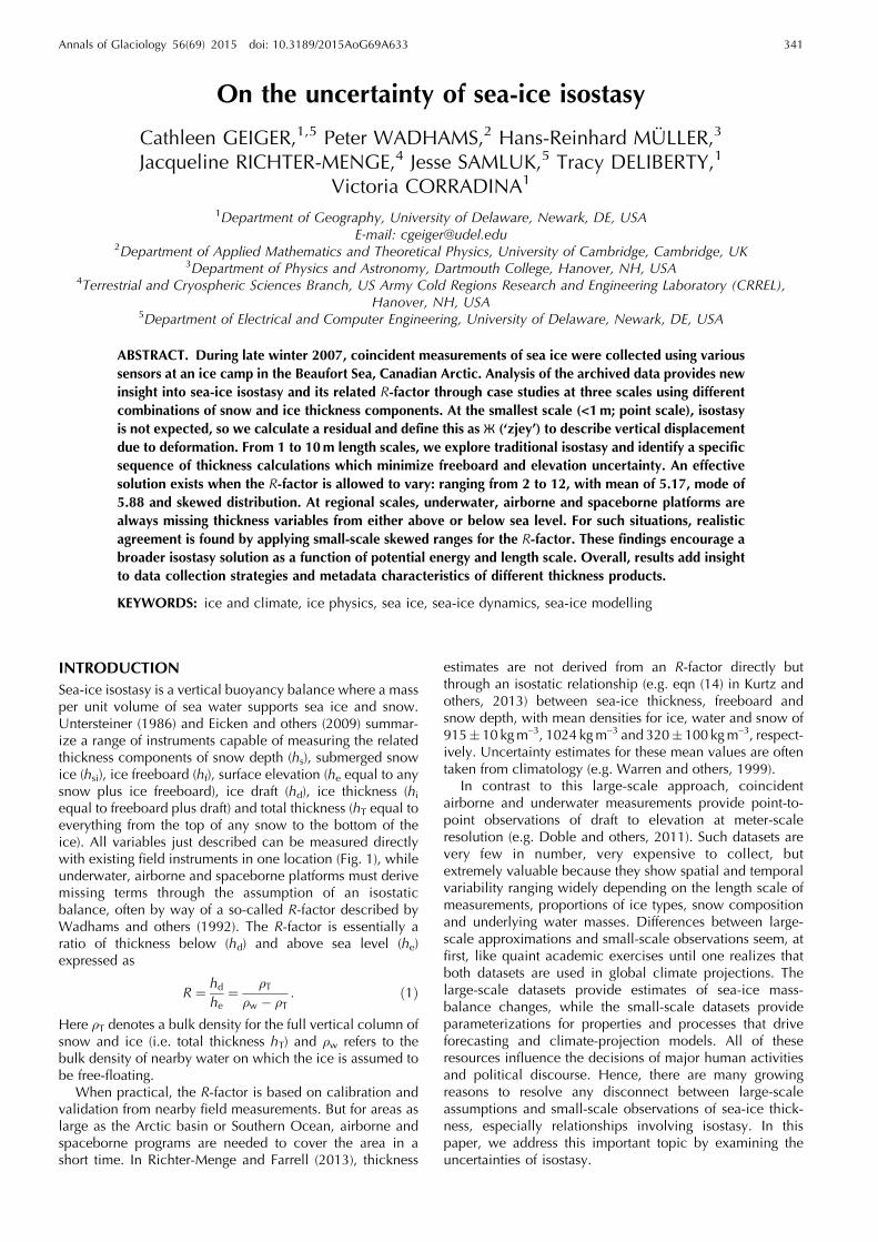
INTRODUCTIONSea-ice isostasy is a vertical buoyancy balance where a massper unit volume of sea water supports sea ice and snow.Untersteiner (1986) and Eicken and others (2009) summar-ize a range of instruments capable of measuring the relatedthickness components of snow depth (hs), submerged snowice (hsi), ice freeboard (hf), surface elevation (he equal to anysnow plus ice freeboard), ice draft (hd), ice thickness (hiequal to freeboard plus draft) and total thickness (hT equal toeverything from the top of any snow to the bottom of theice). All variables just described can be measured directlywith existing field instruments in one location (Fig. 1), whileunderwater, airborne and spaceborne platforms must derivemissing terms through the assumption of an isostaticbalance, often by way of a so-called R-factor described byWadhams and others (1992). The R-factor is essentially aratio of thickness below (hd) and above sea level (he)expressed as

R ¼hdhe¼

�T

�w � �T: ð1Þ

Here �T denotes a bulk density for the full vertical column ofsnow and ice (i.e. total thickness hT) and �w refers to thebulk density of nearby water on which the ice is assumed tobe free-floating.

When practical, the R-factor is based on calibration andvalidation from nearby field measurements. But for areas aslarge as the Arctic basin or Southern Ocean, airborne andspaceborne programs are needed to cover the area in ashort time. In Richter-Menge and Farrell (2013), thickness

estimates are not derived from an R-factor directly butthrough an isostatic relationship (e.g. eqn (14) in Kurtz andothers, 2013) between sea-ice thickness, freeboard andsnow depth, with mean densities for ice, water and snow of915� 10 kgm–3, 1024 kgm–3 and 320�100 kgm–3, respect-ively. Uncertainty estimates for these mean values are oftentaken from climatology (e.g. Warren and others, 1999).

In contrast to this large-scale approach, coincidentairborne and underwater measurements provide point-to-point observations of draft to elevation at meter-scaleresolution (e.g. Doble and others, 2011). Such datasets arevery few in number, very expensive to collect, butextremely valuable because they show spatial and temporalvariability ranging widely depending on the length scale ofmeasurements, proportions of ice types, snow compositionand underlying water masses. Differences between large-scale approximations and small-scale observations seem, atfirst, like quaint academic exercises until one realizes thatboth datasets are used in global climate projections. Thelarge-scale datasets provide estimates of sea-ice mass-balance changes, while the small-scale datasets provideparameterizations for properties and processes that driveforecasting and climate-projection models. All of theseresources influence the decisions of major human activitiesand political discourse. Hence, there are many growingreasons to resolve any disconnect between large-scaleassumptions and small-scale observations of sea-ice thick-ness, especially relationships involving isostasy. In thispaper, we address this important topic by examining theuncertainties of isostasy.

Annals of Glaciology 56(69) 2015 doi: 10.3189/2015AoG69A633 341

We begin by identifying the three largest sources ofvariability. First, snow density (�s) has a larger range thanmean climatological deviations with variability of order100% (e.g. �s�300�300 kgm–3) based on direct measure-ments (e.g. Sturm and others, 2006; Weeks, 2010). Second,the difference between densities of sea water and sea ice (i.e.�w – �i) is high. This seems an unlikely source at first sincesea-water surface density varies little (e.g. 1022�5 kgm–3 inthe SEDNA archive discussed later), <1% relative difference.However, the compiled work on densities by Timco andFrederking (1996) found sea-ice density (�i) between 720 and940 kgm–3 (or <25% relative difference), with an averagevalue of 910 kgm–3. First-year (FY) sea ice varies from 840 to910 kgm–3 above the waterline, and from 900 to 940 kgm–3

below the waterline. Using the rough ranges above, thedifference between highest water density and smallest icedensity reported here is roughly the same size as snowdensity variability (e.g. 1027 – 720=307 kgm–3), with therange of differences similar to snow density variability (e.g.differences between 77 and 307 kgm–3 using examplenumbers above), especially in summer when ice densityvalues decrease as the ice decays structurally during themelting process (Barber, 2005; Timco and Weeks, 2010).Additionally, densities are not normally distributed locally (e.g. Timco and Frederking, 1996; Weeks, 2010) and hence aredifficult to parameterize with standard statistics. In short,density values are highly variable in time and space, and notrepresented well using a climatological mean with associ-ated normally distributed variance. Furthermore, at any timeof the year, sea ice may contain voids where sea waterintrudes, especially in unconsolidated first-year deformed(FYD) ice (i.e. newly formed ridges), with brine channelsbeing the small-scale voids that contain considerable seawater at strongly varying high salinities. Hence, the intrinsic

material property of density for all three materials (snow, ice,water) is responsible for the largest uncertainties in anybuoyancy calculations. Most importantly, there is currentlyno systematic way to non-invasively measure density, withinvasive methods being time-consuming and sparse com-pared to measurements of thickness and area.

The last issue is the validity of isostasy itself. While anisostatic balance for ice exists at some length scale (Timcoand Frederking, 1996), that length scale is not understood,nor do we have a way of characterizing such length scales.Isostasy is a steady-state balance assumed to be more or lesstrue away from pressure ridges and actively deformingfeatures (e.g. Hopkins 1994). But sea-ice thickness issampled (e.g. Wadhams, 1981, 2000) with the largest massfound in the ridged and deformed ice. Additionally, as soonas ice concentrations at any length scale begin to approach80%, a history of mechanical processes invokes lateral iceforces which deform the ice in three dimensions (3-D)through bending, buckling, cracking, folding, grinding,rafting, ridging, shearing and twisting (Thorndike and others,1975). The history of these processes is captured in iceshapes that differentially slide over a slippery ice–waterinterface below, while sticking together by freezing airtemperatures above. In this way, deformation processes workand rework sea-ice thickness over different length scales andre-establish isostasy after each deformation event based onintegrated lateral and vertical interlocking forces over manylength scales (i.e. potentially scale-invariant; Hopkins andothers, 2004). Therefore, there are a number of non-isostaticprocesses that are non-stationary and large enough toaugment thermodynamically grown ice, of order 1–2ma–1,into several possible non-Gaussian (i.e. skewed) thicknessdistributions (e.g. Geiger and others, 2011). Long distributiontails can easily reach and exceed ten times thermodynamicvertical growth. As a result, processes such as sea-icedeformation and drifting snow complicate isostatic balanceat largely unknown and time-varying length scales based ona combination of factors not yet fully understood. Therefore,a strategic starting point begins with a review of theunderlying principles and their associated uncertainties.

Fundamentally, the underlying premise begins with thebasic principle that ice floats. For simplicity, let us considerarctic sea ice which is often composed of columnar ice.Columnar ice looks like tiny hexagonal vertical columns,with a useful surrogate in an academic setting being that ofthe traditional wooden hexagon-beveled pencil. If weimagine a bundle of unsharpened pencils of differentlengths then we can visualize holding that bundle in onehand with all the pencils next to each other. We can use thefingers on our other hand to push on the ends of individualpencils. This is possible because the pencils are nearlyindependent of each other. The hand holding the pencils isapplying a force which creates friction that holds the pencilstogether. When we loosen our grip, we apply less force andthis makes it easier to slide each pencil along the others.This interesting toy model lets us create different surfacesbased on the position of the top and bottom ends of thepencils relative to each other. We can also apply onecommon force to move all the pencils up or down together.Essentially, we are working with a physical model whichsatisfies Newton’s laws which explain how forces balanceand, more specifically, the case of lateral and gravitationalforces – the latter associated with Archimedes’ principleof buoyancy.

Fig. 1. Sea-ice thickness variables and their relationships. Verticalschematic shown with total thickness (T) comprising a composite ofcryospheric materials at the air–sea interface. Different-coloredpathways abstractly describe possible combinations. Pathways arechosen based on instruments and processing algorithms.

Geiger and others: On the uncertainty of sea-ice isostasy342

For real sea ice, there is an added complication that everypiece of ice is partly glued to its neighbors. Some ice piecesare subject to deformation through lateral forces whileothers are pushed up or down due to snow which is falling,blowing and redistributing in large amounts on top of the icewhich is floating on sea water. In such cases, isostaticbalance does not act on a point-by-point basis because seaice is an integrated solid material. Instead, sea ice floatsfreely on sea water with an averaged interconnectedbalance which is valid over some length scale (L). Unlikethe pencil model, the isostatic balance of sea ice includesdifferent materials with different densities, with sea waterbeing the heaviest followed by sea ice, then snow. Thedensity is critical to the buoyancy force balance becausebuoyancy acts in the vertical direction where gravity pullsheavier materials downward, thereby allowing lighter seaice to float on sea water.

Through similar analogies, we begin to understand whythere is a large range of R-factors found by Doble and others(2011) when analyzing small-scale (<1m footprint) meas-urements collected with a multibeam sonar. At larger scales,such as those described by Wadhams and others (1992), R-factors are computed by matching overall probabilitydensity functions of freeboard and draft over long distances.The only way to currently compare results found by Dobleand others (2011) with those by Wadhams and others (1992)is to take a mean R-factor from all the measurementsreported in Doble and others (2011). Unfortunately, theaveraging process removes much of the natural variabilityneeded to understand the processes and length scalesassociated with isostasy (e.g. Geiger and others, 2015).

Given the complexity of the situation, we examineisostasy in this paper from a scaling perspective. Multipleinstruments are clearly needed to create effective data-fusedproducts, but effective approximations are needed becausemost direct measurements are invasive and disrupt thematerial being measured (e.g. drilling). We begin byexpanding upon the underlying traditional mathematicalpremise. We incorporate error propagation to evaluate thefull range of values rather than mean estimates. Becausemany of the variables are not normally distributed, there ismuch to be learned by quantifying natural variations atdifferent scales with different instrument combinations.Next, we evaluate sample data from three different scalesas case studies to determine effective combinations whichminimize uncertainties given assumptions made. Finally, wereassess current thinking and outline a new approach whichtakes into account scale as well as measurement practices.

MATHEMATICAL PREMISEConsider a mass of free-floating ice (mi) over a horizontalarea (A) with the possibility of snow cover either above sealevel (ms) or subject to flooding and refreezing below sealevel (msi). This mass is in isostatic balance with thesurrounding sea water and will displace a certain mass ofsea water (mw) through the relation mw ¼ mi þmsi þms:

When the area observed is not free-floating, there are 3-Dpressures and shearing forces from surrounding structures(e.g. ice, land, waves or tidal surface gradients, etc.). Thevertical component of these forces (Fz) works with or againstgravity (g) to push the floating solid material up or down.Here we define the vertical displacement due to deform-ation from such forces as Ж (pronounced ‘zjey’) and express

the vertical balance of sea ice and snow on sea waterthrough the mass per unit area mathematical relation

mw

A¼ �whw

¼mi þmsi þms

AþFzgA

¼ �ihi þ �sihsi þ �shs þ �TЖ,

ð2Þ

where

�T ¼�ihi þ �sihsi þ �shs

hThT ¼ hi þ hsi þ hsFzgA¼ �TЖ:

ð3Þ

Here � is density and h is thickness, with subscripts w, i, s, siand T representing water, ice, snow, snow ice and total,respectively (Fig. 1). Applying terms defined within sea-iceliterature (e.g. Eicken and others, 2009), we use sea level(z=0) to delineate ice draft (hd) from ice freeboard (hf), withice thickness (hi) equal to the draft plus freeboard. Forcompleteness, we identify elevation (he) equal to any snowplus freeboard. We also identify the term snow ice (subscriptsi) as the flooding and freezing of snow into ice (as is oftenthe case for Antarctic sea ice).

For simplicity in this paper, we assume an Arctic situationwhere snow ice is negligible. Subsequently, we reorganizeour balance into typical arctic thickness combinations(Fig. 1) by substituting hd =hw and hd +hf =hi and notingthat �e is bulk density for elevation as a weighted average ofsnow and freeboard ice such that

�w � �ið Þhd ¼ �ehe þ �TЖ ¼ �ihf þ �shs þ �TЖ: ð4Þ

Using principles of error propagation (e.g. Geiger, 2006), weexpand each term in Eqn (4) into a central-tendency value(denoted by a bar over a variable) and an uncertainty range(denoted with �). We take care not to restrict uncertaintiesto a normal distribution by identifying a distinct lower andupper bound for each variable, especially since boththickness and density are known for their lack of symmetryabout a mean value. At length scales (L) where isostasy isassumed valid, we set ЖðLÞ ¼ 0. In this way, Eqn (4)expresses solutions in a form typically seen in the literature(e.g. Eqn (1)) for central-tendency solutions for the R-factor(R) plus or minus variability. Mathematically, this isexpressed as (details in Eqns (A1–A3) in Appendix)

R ¼ R��R; R ¼hdhe¼

�e�w � �i

ð5Þ

�R ¼ R

ffiffiffiffiffiffiffiffiffiffiffiffiffiffiffiffiffiffiffiffiffiffiffiffiffiffiffiffiffiffiffiffiffiffiffiffiffiffiffiffiffiffiffiffiffiffiffiffiffiffiffiffiffiffiffiffiffiffi

��e

�e

� �2

þ��w2 þ��i2

�w � �ið Þ2

!vuut : ð6Þ

Two related factors are similarly derived for ratios of totalthickness-to-draft and total thickness-to-elevation with thesame propagated uncertainty as Eqn (6).

RT=D ¼hThd¼hd þ hehd

¼ 1þ1R; ð7Þ

RT=E ¼hThe¼hd þ hehe

¼ 1þ R, ð8Þ

where subscripts T/D and T/E signify total-to-draft and total-to-elevation respectively. Unlike Eqn (5), Eqns (7) and (8) do

Geiger and others: On the uncertainty of sea-ice isostasy 343

not have independent numerator and denominator, but theydo provide the practical relationships often invoked forunderwater, airborne and spaceborne measurements whichuse these relationships to estimate a total thickness based onsome proportion of measured draft or elevation. Insubsequent sections, we invoke different combinations ofvariables using Eqns (5–8) to determine which solutionsprovide the least uncertainty. Our goal with such aformulation is to identify the most accurate pathways(Fig. 1) to improve data collection strategies.

METHODOLOGYWe use an archive from the International Polar Year fieldexperiment called the Sea-ice Experiment: Dynamic Natureof the Arctic (SEDNA; Hutchings and others, 2008, 2011).Specific data include regional submarine upward-lookingsonar returns (Geiger and others, 2011; Wadhams andothers, 2011), electromagnetic (EM) induction sea-icethickness retrievals using a Geonics EM-31-MK2 (hereafterreferred to as EM-31), snow depth using a MagnaProbe

(Sturm and others, 2006), snow density measurements anddrilled holes (Figs 2 and 3).

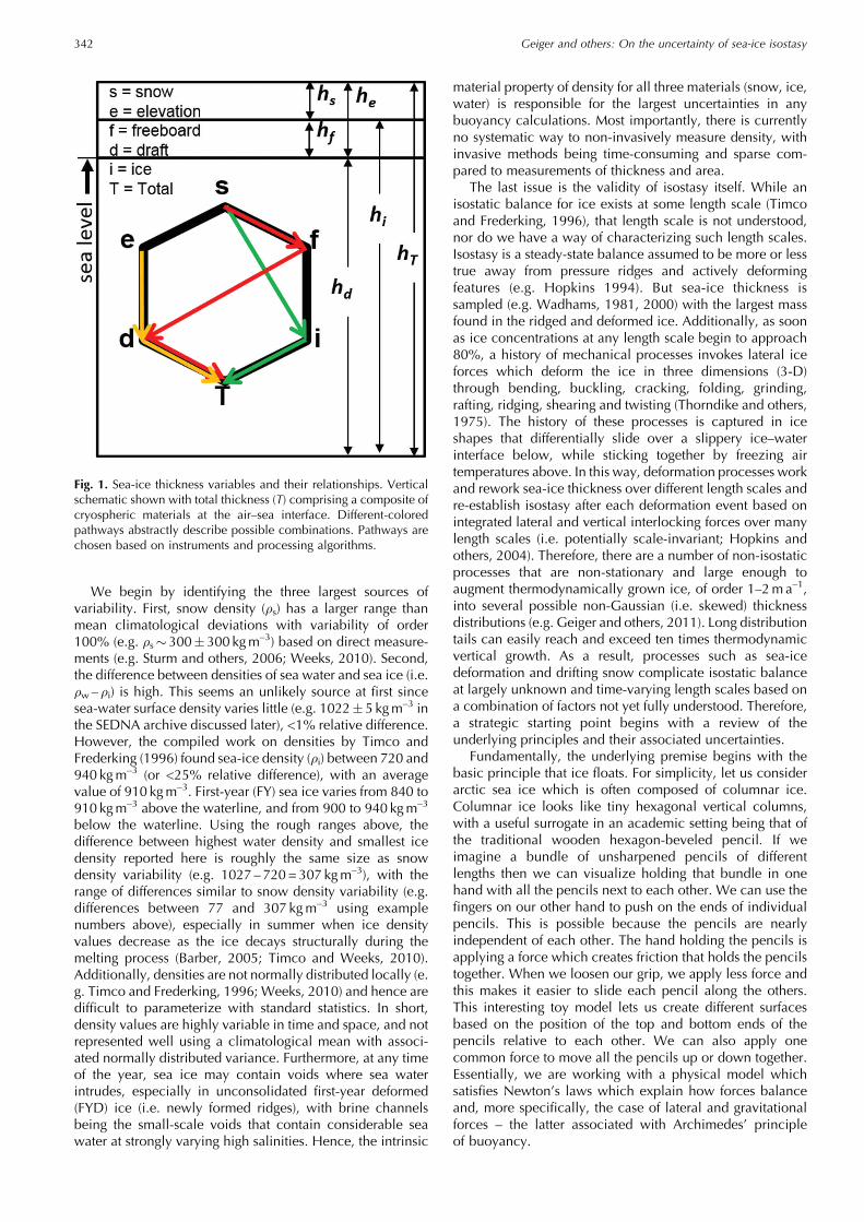
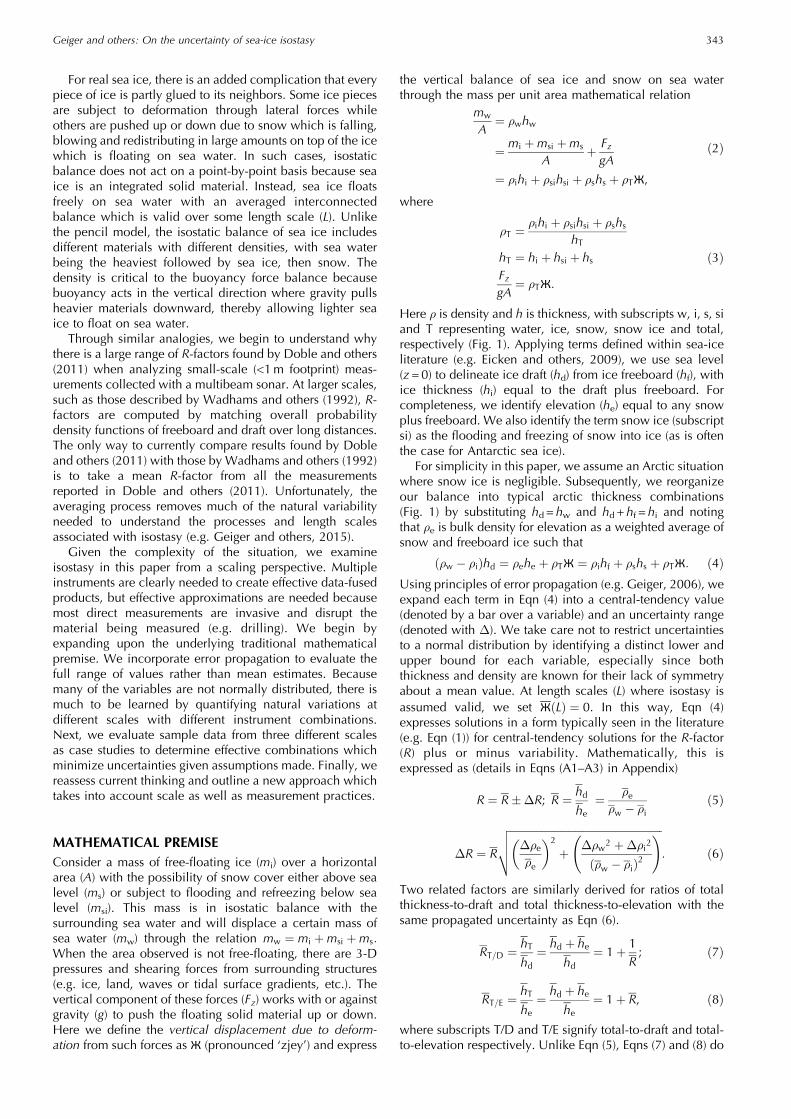
Data processingThe camp layout (Fig. 3) provides a reference of icestructures for (1) drillhole validation sites at the point scale,(2) EM thickness profiles at intermediate scale with 5mspacing over 6 km long spokes, and (3) submarine upward-looking sonar profiles (Fig. 2) spanning the regional scale.Submarine sonar measurements were bound within a surveybox of length 20 km (2�104m) on each side (Fig. 2b) andinclude five passes through the camp survey area includingone pass beneath line 7 (Fig. 3a). All three datasets werecollected within 2 weeks of each other. Data collected andanalyzed during the ice camp from 3 to 7 April areconsidered coincident measurements because the thicknessarray did not deform noticeably during that 4 day windowbased on direct and airborne observations. The submarinedata, however, were collected 2 weeks prior to the fieldcamp. The time frame from end of March to beginning ofApril is too short to be noticeably different in terms ofthermodynamic growth or melt, but certainly different atpoint-by-point locations due to deformation processes. It isfor this reason that a statistical approach is used to relatesubmarine results to ice camp measurements with these twodatasets considered quasi-coincident.

Data-processing methods are provided below, with eachmeasured value reported with its uncertainty which ispropagated into subsequent calculations. Density values areknown explicitly for a few points for snow but inferred fromthe ranges cited in the introduction otherwise. Ice density is

Fig. 2. Submarine survey. (a) Geographic region with RADARSAT-1image centered on ice camp on 18 March 2007. Multi-year icedepicted by whiter pixels, first-year ice by darker pixels. Ice cover isnearly 100% concentration with very narrow leads of open waterwhich refreeze quickly. Red box identifies the study area shown in(b). (b) Submarine tracks superimposed on small section ofRADARSAT-1 image from (a). Hours of the day on 18 March2007 (in UTC) segmented (by color) for the submarine track.Arrows bear true north.

Fig. 3.Arctic ice camp survey. (a) Lines superimposed on photographtaken from light-wing aircraft at oblique angle over 1000m long legs.Conditions during the thickness survey from 1 to 7 April 2007 arewell represented, with no open water along any leg. Arrow bearingtrue north. (b) Camp layout with 8 ft (2.44m) tall plywood huts forscale reference. (Photograph by Bruce Elder, CRREL.)

Geiger and others: On the uncertainty of sea-ice isostasy344

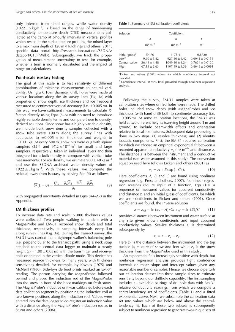
only inferred from cited ranges, while water density(1022�5 kgm–3) is based on the range of time-varyingconductivity–temperature–depth (CTD) measurements col-lected at the camp at 6 hourly intervals in vertical profileswhich rested at the surface before profiling the mixed layerto a maximum depth of 120m (Hutchings and others, 2011;specific data portal http://research.iarc.uaf.edu/SEDNA/dataport/CTD_Wilk/). Subsequently, we track the propa-gation of measurement uncertainty to test, for example,whether a term is normally distributed and the impact ofrange on calculations.

Point-scale isostasy testingThe goal at this scale is to test sensitivity of differentcombinations of thickness measurements to natural vari-ability. Using a 0.10m diameter drill, holes were made atvarious locations along the six survey lines (Fig. 3a) withproperties of snow depth, ice thickness and ice freeboardmeasured to centimeter vertical accuracy (i.e. �0.005m). Inthis way, we have sufficient measurements to calculate R-factors directly using Eqns (5–8) with no need to introducehighly variable density terms and compare these to density-derived solutions. Since snow has a highly variable density,we include bulk snow density samples collected with asnow tube every 100m along the survey lines withaccuracies to �0.005m for thickness and weights to�0.001 kg. At every 500m, snow pits were dug with squaresamplers (32.4 and 97.2� 10–6m3 for small and largesamplers, respectively) taken in individual layers and thenintegrated for a bulk density to compare with vertical tubemeasurements. For ice density, we estimate 900�40 kgm–3

and use the SEDNA archived water density values of1022�5 kgm–3. With these values, we compute theresidual away from isostasy by solving Eqn (4) as follows:

Ж L ¼ 0ð Þ ¼�w � �ið Þhd � �ihf � �shs

�Tð9Þ

with propagated uncertainty detailed in Eqns (A4–A7) in theAppendix.

EM thickness profilesTo increase data rate and scale, >1000 thickness valueswere collected. Two people walking in tandem with aMagnaProbe and EM-31 recorded snow depth and totalthickness, respectively, at sampling intervals every 5malong survey lines (Fig. 3a). During this transect survey, theEM-31 was carried like a tightrope walker’s balancing pole(i.e. perpendicular to the transect path) using a neck strapattached to the central data logger to maintain a steadyheight (z0 = 1.00�0.05m) with the transmitter and receivercoils orientated in the vertical dipole mode. This device hasmeasured sea-ice thickness for many years, with thicknesssensitivities detailed, for example, by Kovacs (1975) andMcNeill (1980). Side-by-side boot prints marked an EM-31reading. The person carrying the MagnaProbe followedbehind and placed the induction rod of the MagnaProbeinto the snow in front of the boot markings on fresh snow.The MagnaProbe’s inductive unit was calibrated before eachdata collection segment by positioning the inductive coil attwo known positions along the induction rod. Values wereentered into the data logger to co-register an induction valuewith a distance along the MagnaProbe’s induction rod as inSturm and others (2006).

Following the survey, EM-31 samples were taken atcalibration sites where drilled holes were made. The drilledholes included snow depth (with MagnaProbe) and icethickness (with hand drill) both to centimeter accuracy (i.e.�0.005m). At some calibration locations, the EM-31 washeld at two different heights (carrying height around 1m andground) to include beamwidth effects and orientationrelative to local ice features. Subsequent data processing isdone in two steps: (1) resolve thickness; and (2) identifyisostatic components. First, the EM-31 requires calibrationfor which we choose an empirical exponential fit between arecorded apparent conductivity �a (mSm–1) and distance z.The distance z is between the instrument and a conductivematerial (sea water assumed in this study). The conversionequation used here follows Eicken and others (2001) as

�a ¼ Aþ B exp ð� CzÞ: ð10Þ

Here coefficients A, B and C are found using nonlinearregression (e.g. Press and others, 2007). Nonlinear regres-sion routines require input of a function, Eqn (10), asequence of measured values for apparent conductivityand distance z, and an initial guess of coefficients, for whichwe use coefficients in Eicken and others (2001). Oncecoefficients are found, the inverse solution

z ¼ zref � ln ð�a � AÞ=C; zref ¼ ln ðBÞ=C ð11Þ

provides distance z between instrument and water surface atany site given known coefficients and input apparentconductivity values. Sea-ice thickness zi is determinedsubsequently by

zi ¼ z � z0 � zs: ð12Þ

Here z0 is the distance between the instrument and the topsurface (a mixture of snow and ice) while zs is the snowthickness from the MagnaProbe used in this study.

An exponential fit is increasingly sensitive with depth, butnonlinear regression analysis provides tight confidenceintervals on mean slope and intercept values given anyreasonable number of samples. Hence, we choose to perturbour calibration dataset into three sample sizes to estimatesensitivity beyond our drillhole capability. The first samplingincludes all available pairings of drillhole data with EM-31relative conductivity readings from which we compute acentral-tendency set of coefficients (Table 1) and a fittedexponential curve. Next, we subsample the calibration dataset into values which are below and above the central-tendency fit. Each of these two subsets is subsequentlysubject to nonlinear regression to generate two unique sets of

Table 1. Summary of EM calibration coefficients

Solution Coefficient

A B C

mSm–1 mSm–1 m–1

Initial guess* 54.70 1178.41 0.8720Low† 9.90� 5.82 927.80� 9.42 0.6943�0.0158Central value 26.48� 4.48 1049.40� 6.24 0.7624�0.0120High 67.13� 2.63 1107.19� 3.38 0.8649�0.0081

*Eicken and others (2001) values for which confidence interval notprovided.† Confidence interval at 95% level provided through nonlinear regressionanalysis.

Geiger and others: On the uncertainty of sea-ice isostasy 345

coefficients which we call the low and high solutions(Table 1). This approach provides a very tight set of fittedcurves where data values span the exponential fit (Fig. 5a,further below), but with a growing uncertainty beyond thedata-availability range. Resulting thickness values are con-catenated together to form a single thickness profile.

Isostasy calculations for these data are computed using acoupled set of equations to render the unmeasured terms ofdraft, freeboard, and elevation thickness (Fig. 1). Since thereare insufficient known variables to test isostasy, we need tointroduce an assumption. Counter to the point-scale testsearlier, we take the opposite, and currently traditional,approach, which hypothesizes that an EM footprint is ofsufficient size L such that ЖðLÞ ¼ 0. In other words, weassume that isostatic balance exists at a scale around 5mwhich is the length scale of the sampling intervals based onthe coil separation distance of the EM-31. We track theuncertainties to identify the solution pathways which renderthe smallest uncertainties starting from Eqn (9) and inputdirectly measured snow and total thickness values:

hd ¼�ihT � �i � �sð Þhs

�w

hf ¼ hT � ðhd þ hsÞ

he ¼ hf þ hs:

ð13Þ

Such a solution is often the only practical option available,so we test this scenario to address best practices wheninvoking this approximation knowing that non-isostaticconditions are probably present but so are other complica-tions which we show and discuss later.

Submarine upward-looking sonar profilesAround 2� 105m (200 km) of sea-ice draft measurementswere gathered by the Royal Navy submarine HMS Tireless inthe vicinity of the ice camp on 18 March 2007 (Fig. 2).Processing was completed following Geiger and others(2011), Wadhams and others (2011) and Wadhams (2012).Mean ice draft values were subsequently added to theSEDNA archive (Hutchings and others, 2011), with biasesreported primarily from the sonar’s variable footprint due tothe 3° beamwidth. For simplicity here, we use the reportedsubmarine draft ‘as is’ to explore the variability of elevationvalues that may result given R-factor estimates derived fromice camp survey estimates of isostasy. In this way, we testthe impact of propagated uncertainties when creatingcombined data products. As such, the submarine archiveserves as an applied case study for consistency betweenscales within the region (Fig. 2). Similar statistical tests canbe repeated with respect to satellite and airborne remote-sensing data and numerical models.

The relevant conversions are as follows. First, weconstruct thickness distributions of total thickness and draftfor ice camp in situ measurements. We identify the mode ofthe distributions of total thickness and draft, and subse-quently construct a ratio between these modes to computethe total-to-draft R-factor following Eqn (7). We apply thecomputed R-factor to the submarine draft to estimate a totalthickness and elevation for submarine results. We call thisapproach the ‘thermodynamic-mode solution’ as in Geigerand others (2011). This solution is preferred because theprimary mode during the SEDNA experiment corresponds tofirst-year level ice and its accumulated snow cover.Thermodynamically grown ice can be approximated with a

degree-day algorithm, and precipitation on level ice is farless variable than on deformed ice types. These two factorssupport a statistical solution with low uncertainties relative tomost approximations currently used. Later on, we comparethis thermodynamic solution to low, central-tendency andhigh R-factor solutions based on slopes derived from isostasysolutions from drillhole data using the relation

he ¼hdR; hT ¼ hd þ he: ð14Þ

The submarine case study examines elevation solutions fortwo reasons. First, draft is the larger value such that variationsin elevation are expected to be small in comparison toairborne and spaceborne retrievals where elevation errorswill propagate to larger draft errors. Second, we can directlycompare the elevation from submarine thickness retrievals inthe area of the ice camp and ascertain regional consistency.We do this by comparing the elevation results of the entirearea traversed by the submarine with the portions whichpassed through the area surveyed during the ice camp.Similar comparisons already provide strong agreement fordraft and total thickness of this same dataset (Geiger andothers, 2011).

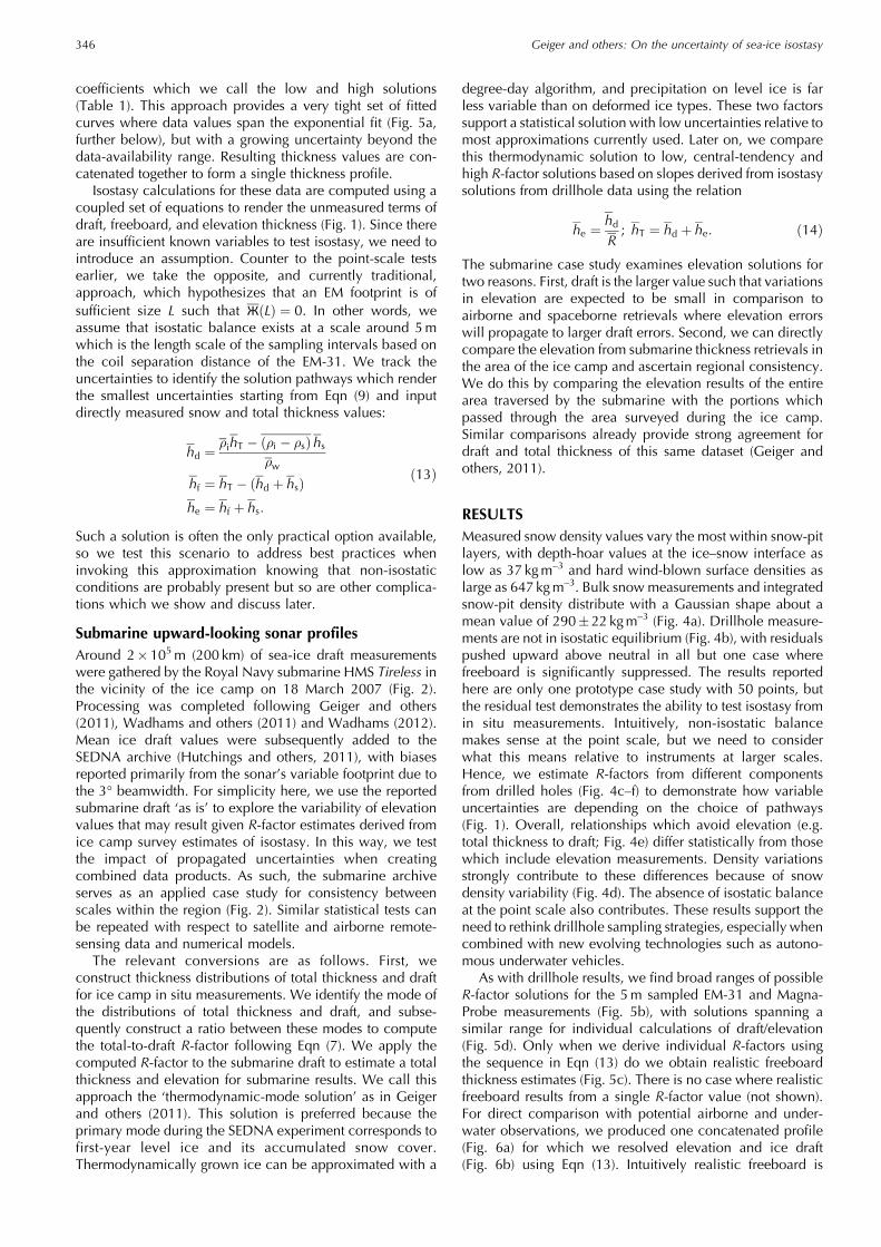
RESULTSMeasured snow density values vary the most within snow-pitlayers, with depth-hoar values at the ice–snow interface aslow as 37 kgm–3 and hard wind-blown surface densities aslarge as 647 kgm–3. Bulk snow measurements and integratedsnow-pit density distribute with a Gaussian shape about amean value of 290�22 kgm–3 (Fig. 4a). Drillhole measure-ments are not in isostatic equilibrium (Fig. 4b), with residualspushed upward above neutral in all but one case wherefreeboard is significantly suppressed. The results reportedhere are only one prototype case study with 50 points, butthe residual test demonstrates the ability to test isostasy fromin situ measurements. Intuitively, non-isostatic balancemakes sense at the point scale, but we need to considerwhat this means relative to instruments at larger scales.Hence, we estimate R-factors from different componentsfrom drilled holes (Fig. 4c–f) to demonstrate how variableuncertainties are depending on the choice of pathways(Fig. 1). Overall, relationships which avoid elevation (e.g.total thickness to draft; Fig. 4e) differ statistically from thosewhich include elevation measurements. Density variationsstrongly contribute to these differences because of snowdensity variability (Fig. 4d). The absence of isostatic balanceat the point scale also contributes. These results support theneed to rethink drillhole sampling strategies, especially whencombined with new evolving technologies such as autono-mous underwater vehicles.

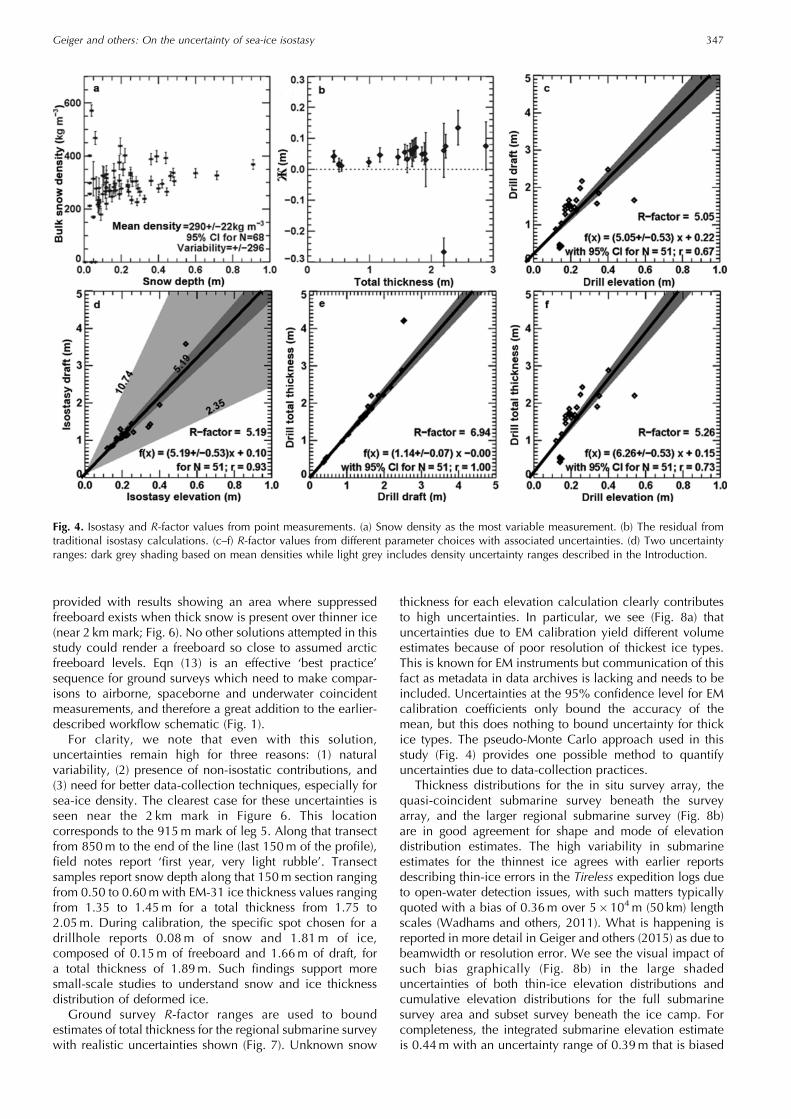
As with drillhole results, we find broad ranges of possibleR-factor solutions for the 5m sampled EM-31 and Magna-Probe measurements (Fig. 5b), with solutions spanning asimilar range for individual calculations of draft/elevation(Fig. 5d). Only when we derive individual R-factors usingthe sequence in Eqn (13) do we obtain realistic freeboardthickness estimates (Fig. 5c). There is no case where realisticfreeboard results from a single R-factor value (not shown).For direct comparison with potential airborne and under-water observations, we produced one concatenated profile(Fig. 6a) for which we resolved elevation and ice draft(Fig. 6b) using Eqn (13). Intuitively realistic freeboard is

Geiger and others: On the uncertainty of sea-ice isostasy346

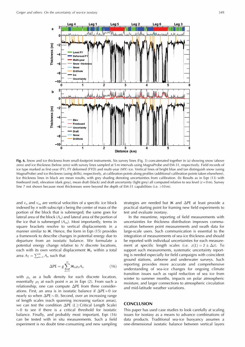
provided with results showing an area where suppressedfreeboard exists when thick snow is present over thinner ice(near 2 km mark; Fig. 6). No other solutions attempted in thisstudy could render a freeboard so close to assumed arcticfreeboard levels. Eqn (13) is an effective ‘best practice’sequence for ground surveys which need to make compar-isons to airborne, spaceborne and underwater coincidentmeasurements, and therefore a great addition to the earlier-described workflow schematic (Fig. 1).

For clarity, we note that even with this solution,uncertainties remain high for three reasons: (1) naturalvariability, (2) presence of non-isostatic contributions, and(3) need for better data-collection techniques, especially forsea-ice density. The clearest case for these uncertainties isseen near the 2 km mark in Figure 6. This locationcorresponds to the 915m mark of leg 5. Along that transectfrom 850m to the end of the line (last 150m of the profile),field notes report ‘first year, very light rubble’. Transectsamples report snow depth along that 150m section rangingfrom 0.50 to 0.60m with EM-31 ice thickness values rangingfrom 1.35 to 1.45m for a total thickness from 1.75 to2.05m. During calibration, the specific spot chosen for adrillhole reports 0.08m of snow and 1.81m of ice,composed of 0.15m of freeboard and 1.66m of draft, fora total thickness of 1.89m. Such findings support moresmall-scale studies to understand snow and ice thicknessdistribution of deformed ice.

Ground survey R-factor ranges are used to boundestimates of total thickness for the regional submarine surveywith realistic uncertainties shown (Fig. 7). Unknown snow

thickness for each elevation calculation clearly contributesto high uncertainties. In particular, we see (Fig. 8a) thatuncertainties due to EM calibration yield different volumeestimates because of poor resolution of thickest ice types.This is known for EM instruments but communication of thisfact as metadata in data archives is lacking and needs to beincluded. Uncertainties at the 95% confidence level for EMcalibration coefficients only bound the accuracy of themean, but this does nothing to bound uncertainty for thickice types. The pseudo-Monte Carlo approach used in thisstudy (Fig. 4) provides one possible method to quantifyuncertainties due to data-collection practices.

Thickness distributions for the in situ survey array, thequasi-coincident submarine survey beneath the surveyarray, and the larger regional submarine survey (Fig. 8b)are in good agreement for shape and mode of elevationdistribution estimates. The high variability in submarineestimates for the thinnest ice agrees with earlier reportsdescribing thin-ice errors in the Tireless expedition logs dueto open-water detection issues, with such matters typicallyquoted with a bias of 0.36m over 5�104m (50 km) lengthscales (Wadhams and others, 2011). What is happening isreported in more detail in Geiger and others (2015) as due tobeamwidth or resolution error. We see the visual impact ofsuch bias graphically (Fig. 8b) in the large shadeduncertainties of both thin-ice elevation distributions andcumulative elevation distributions for the full submarinesurvey area and subset survey beneath the ice camp. Forcompleteness, the integrated submarine elevation estimateis 0.44m with an uncertainty range of 0.39m that is biased

Fig. 4. Isostasy and R-factor values from point measurements. (a) Snow density as the most variable measurement. (b) The residual fromtraditional isostasy calculations. (c–f) R-factor values from different parameter choices with associated uncertainties. (d) Two uncertaintyranges: dark grey shading based on mean densities while light grey includes density uncertainty ranges described in the Introduction.

Geiger and others: On the uncertainty of sea-ice isostasy 347

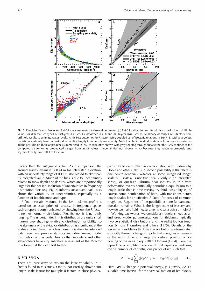
thicker than the integrated value. As a comparison, theground survey estimate is 0.41m for integrated elevation,with an uncertainty range of 0.17m also biased thicker thanits integrated value. Much of the bias is due to uncertaintiesrelated to snow depth and density, which are proportionallylarger for thinner ice. Inclusion of uncertainties in frequencydistribution plots (e.g. Fig. 8) informs subsequent data usersabout the variability of uncertainties, especially as afunction of ice thickness and type.

R-factor variability found in the EM thickness profile isbased on an assumption of isostasy. In frequency space,such a report is communicated by showing how the R-factoris neither normally distributed (Fig. 8c) nor is it narrowlyranging. The uncertainties in this distribution are quite small(narrow grey shading) relative to distribution variability, sothe skewness of the R-factor distribution is significant at thescales studied here. For clear communication to intendeddata users, we provide statistics including mean, mode,distribution and uncertainties so that modelers and otherstakeholders have a quantitative assessment of the R-factorin a form that they can test further.

DISCUSSIONThere are three ways to explain the large variability in R-factors found in this study. One is that isostasy above somelength scale is true for multiple R-factors in close physical

proximity to each other in corroboration with findings byDoble and others (2011). A second possibility is that there isone central-tendency R-factor at some integrated lengthscale but isostasy is not true locally (only in an integratedsense), or quasi-equilibrium near isostasy is true withdeformation events continually perturbing equilibrium to alength scale that is time-varying. A third possibility is, ofcourse, some combination of both, with transitions acrosslength scales for an effective R-factor for areas of commonroughness. Regardless of the possibilities, one fundamentalquestion remains: What is the length scale of isostasy andhow do wemake field measurements to test such a principle?

Working backwards, we consider a modeler’s need as anend user. Model parameterizations for thickness typicallyinvolve statistical distributions and the redistribution func-tion � from Thorndike and others (1975). Details of theforces responsible for thickness redistribution are formulatedexplicitly through changes in potential energy as a measureof the work done to change the vertical position of icefloating on water as in eqn (10) of Hopkins (1994). Here, wereproduce a simplified version of that equation, indexingover a number of N contiguous pieces of ice such that

�PE ¼ gXN

n¼1vn�t½ ��nAn � vns�t½ ��wAnsð Þ ð15Þ

Here �PE is change in potential energy, g is gravity, �t is asuitable time interval for the vertical motion of ice blocks,

Fig. 5. Resolving MagnaProbe and EM-31 measurements into isostatic estimates. (a) EM-31 calibration results relative to coincident drillholevalues for different ice types of first-year (FY) ice, FY deformed (FYD) and multi-year (MY) ice. (b) Summary of ranges of R-factors fromdrillhole results to estimate water levels. (c, d) Best outcomes for R-factor using coupled set of isostatic relations in Eqn (13) with a large butrealistic uncertainty based on natural variability largely from density uncertainty. Note that the individual isostatic solutions are as varied asall the possible drillhole approaches summarized in (b). Uncertainties shown with grey shading throughout at either the 95% confidence forcomputed values or as propagated ranges from input values. Uncertainties not shown in (c) because they range enormously andasymmetrically from <0.1m to >1m.

Geiger and others: On the uncertainty of sea-ice isostasy348

and vn and vns are vertical velocities of a specific ice blockindexed by n with subscript s being the center of mass of theportion of the block that is submerged; the same goes forlateral area of the block (An) and lateral area of the portion ofthe ice that is submerged (Ans). Most importantly, terms insquare brackets resolve to vertical displacements in amanner similar to Ж. Hence, the form in Eqn (15) providesa framework to describe changes in potential energy due todeparture from an isostatic balance. We formulate apotential energy change relative to N discrete locations,each with its own vertical displacement Жn within a totalarea AT ¼

PNn¼1 An such that

�PE ¼ gXN

n¼1Жn�nAn ð16Þ

with �n as a bulk density for each discrete location,essentially �T at each point n as in Eqn (2). From such arelationship, one can compute �PE from three consider-ations. First, an area is in isostatic balance if �PE =0 (ornearly so when �PE� 0). Second, over an increasing rangeof length scales (each spanning increasing surface areas),we can test the condition �PE (L�Critical Length Scale)�0 to see if there is a critical threshold for isostaticbalance. Finally, and probably most important, Eqn (16)can be tested with in situ measurements. Such a fieldexperiment is no doubt time-consuming and new sampling

strategies are needed but Ж and �PE at least provide apractical starting point for framing new field experiments totest and evaluate isostasy.

In the meantime, reporting of field measurements withuncertainties for thickness distribution improves commu-nication between point measurements and swath data forlarge-scale users. Such communication is essential to theintegration of measurements of sea-ice thickness and shouldbe reported with individual uncertainties for each measure-ment at specific length scales (i.e. zðLÞ ¼ z��z). Tosupport such measurements, systematic uncertainty report-ing is needed especially for field campaigns with coincidentground stations, airborne and underwater surveys. Suchreporting provides more accurate and comprehensiveunderstanding of sea-ice changes for ongoing climatetransition issues such as rapid reduction of sea ice fromwinter to summer months, impacts on polar atmosphericmoisture, and larger connections to atmospheric circulationand mid-latitude weather variations.

CONCLUSIONThis paper has used case studies to look carefully at scalingissues for isostasy as a means to advance combinations ofdata products. Traditional sea-ice buoyancy assumes aone-dimensional isostatic balance between vertical layers

Fig. 6. Snow and ice thickness from small-footprint instruments. Six survey lines (Fig. 3) concatenated together in (a) showing snow (abovezero) and ice thickness (below zero) with survey lines sampled at 5m intervals using MagnaProbe and EM-31, respectively. Field records ofice type marked as first-year (FY), FY deformed (FYD) and multi-year (MY) ice. Vertical lines of bright blue and tan distinguish snow (usingMagnaProbe) and ice thickness (using drills), respectively, at calibration points along profiles (additional calibration points taken elsewhere).Ice thickness lines in black are mean results, with grey shading denoting uncertainties from calibration. (b) Results as in Eqn (13) withfreeboard (red), elevation (dark grey), mean draft (black) and draft uncertainty (light grey) all computed relative to sea level (z=0m). Surveyline 7 not shown because most thicknesses were beyond the depth of EM-31 capabilities (i.e. >10m).

Geiger and others: On the uncertainty of sea-ice isostasy 349

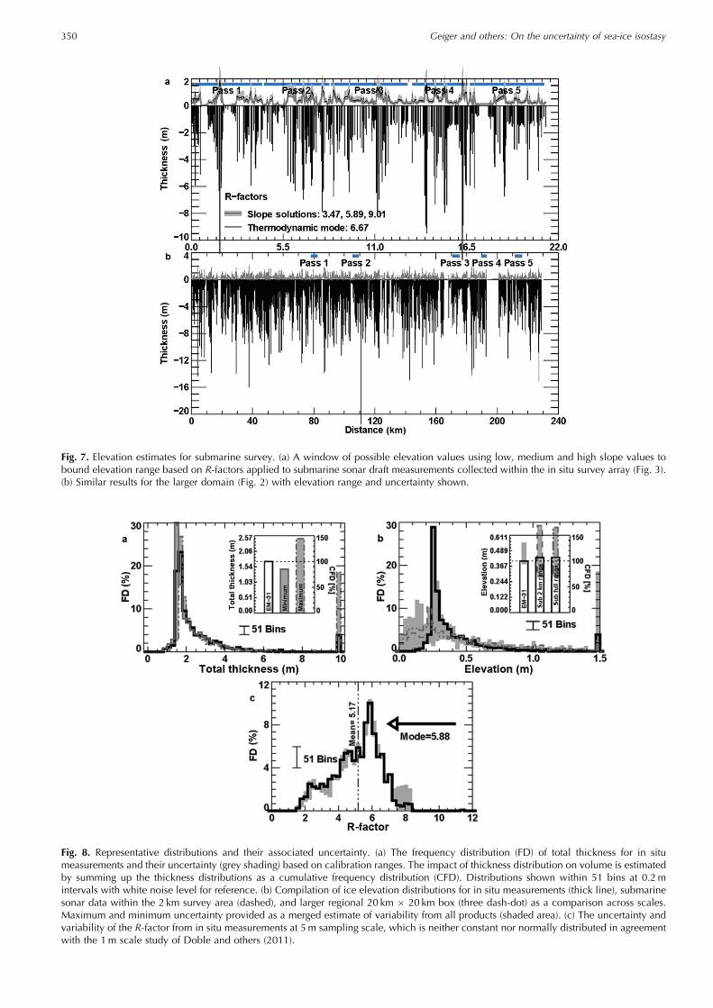
Fig. 7. Elevation estimates for submarine survey. (a) A window of possible elevation values using low, medium and high slope values tobound elevation range based on R-factors applied to submarine sonar draft measurements collected within the in situ survey array (Fig. 3).(b) Similar results for the larger domain (Fig. 2) with elevation range and uncertainty shown.

Fig. 8. Representative distributions and their associated uncertainty. (a) The frequency distribution (FD) of total thickness for in situmeasurements and their uncertainty (grey shading) based on calibration ranges. The impact of thickness distribution on volume is estimatedby summing up the thickness distributions as a cumulative frequency distribution (CFD). Distributions shown within 51 bins at 0.2mintervals with white noise level for reference. (b) Compilation of ice elevation distributions for in situ measurements (thick line), submarinesonar data within the 2 km survey area (dashed), and larger regional 20 km � 20 km box (three dash-dot) as a comparison across scales.Maximum and minimum uncertainty provided as a merged estimate of variability from all products (shaded area). (c) The uncertainty andvariability of the R-factor from in situ measurements at 5m sampling scale, which is neither constant nor normally distributed in agreementwith the 1m scale study of Doble and others (2011).

Geiger and others: On the uncertainty of sea-ice isostasy350

of water, ice and snow. Findings here show that thisassumption should be extended to include lateral forcesresulting from deformation, with this study framing themathematics to begin exploring this topic and supportmore research. In particular, we recommend the develop-ment of new best practices in field measurements whichsupport process model experiments involving Ж andchanges in potential energy. Process models are neededto characterize isostatic length scales in conjunction withtraditional thickness distribution and the redistributionfunction (so-called Thorndike � parameter). Strong vari-ability in bulk densities of different cryospheric materialsand large variations in snow depth strongly contribute to anR-factor that is not normally distributed nor necessarily inisostatic balance locally. We therefore encourage thedevelopment of generalized buoyancy models to studyperturbations from isostasy as a function of dynamics andtime-varying length scales.

In summary, small-scale point measurements (<1m)provide invaluable information about the distribution ofsea-ice buoyancy from a 3-D perspective. At scales from1 to 10m, the steps outlined in Eqn (13) provide goodapproximations for freeboard elevation by determiningunknowns with low uncertainties. Likewise for large-scaleunderwater vehicles, a good estimate of thermodynamicthickness provides a low uncertainty estimate for elevationin the absence of snow thickness information. Airborne andspaceborne solutions benefit from similar approaches assnow-penetrating radars improve and snow-blowing processmodels over rough ice are advanced. But in the end, themost effective advancements will come from small-scale(0.1–100m) buoyancy-mapping techniques which providegreater insight into the spatial distribution of the intrinsicproperty of density. This is an ambitious challenge, but thedata clearly indicate that such an approach is warranted ifwe are to reduce the uncertainties.

ACKNOWLEDGEMENTSThe US National Science Foundation (NSF) providedsupport through ARC-1107725 (University of AlaskaFairbanks), ARC-0611991 (CRREL), ARC-0612105 andARC-1107725 (University of Delaware). Submarine scienceteam supported through the DAMOCLES (DevelopingArctic Modeling and Observing Capabilities for Long-termEnvironmental Studies) project and Office of NavalResearch. Logistics made possible through J. Gossett (USArctic Submarine Laboratory), F. Karig (University ofWashington) and the US Navy. We thank N. Hughes(Norwegian Meteorological Institute), A. Turner, K.A. Giles(University College London) and R. Harris for participationin ground surveys, with special remembrance for K.A. Gilesand R. Harris (NSF-sponsored PolarTREC teacher). TheInternational Space Science Institute is acknowledged forcollaborative project No. 169, and R. Kwok (Jet PropulsionLaboratory, Pasadena, CA) for discussions on the long-termvalue of field measurements. Undergraduate studentsT. Mattraw, S. Sood and S. Streeter (classes of 2011,2012 and 2013) participated in analysis through theDartmouth Women In Science Project (WISP). C.G. alsosupported by the College of Earth, Ocean & Environment,University of Delaware, and M. Hilchenbach (MPSFellowship Program).

REFERENCESBarber DG (2005) Microwave remote sensing, sea ice and Arctic

climate. Phys. Can., 61, 105–111Doble MJ, Skouroup H, Wadhams P and Geiger CA (2011) The

relation between Arctic sea ice surface elevation and draft: a casestudy using coincident AUV sonar and airborne scanning laser.J. Geophys. Res.,116(C8), C00E03 (doi: 10.1029/2011JC007076)

Eicken H, Tucker WB III and Perovich DK (2001) Indirectmeasurements of the mass balance of summer Arctic sea icewith an electromagnetic induction technique. Ann. Glaciol., 33,194–200 (doi: 10.3189/172756401781818356)

Eicken H, Gradinger R, Salganek M, Shirasawa K, Perovich D andLeppäranta M eds (2009) Field techniques for sea ice research.University of Alaska Press, Fairbanks, AK

Geiger CA (2006) Propagation of uncertainties in sea ice thicknesscalculations from basin-scale operational observations. CRRELTech. Rep. TR-06-16 http://acwc.sdp.sirsi.net/client/search/asset/1001690

Geiger CAand9 others (2011) A case study testing the impact of scaleon Arctic sea ice thickness distribution. Proceedings of the 20thIAHR International Symposium on Ice, 14–18 June 2010, Lahti,Finland. International Association for Hydro-Environment Engin-eering and Research, Madrid (doi: 10.13140/2.1.2890.3366)

Geiger CA, Müller H-R, Samluk JP, Bernstein ER and Richter-MengeJ (2015) Impact of spatial aliasing on sea-ice thickness measure-ments. Ann Glaciol., 56(69) (see paper in this issue) (doi:10.3189/2015AoG69A644)

Giles KA, Laxon SW and Ridout AL (2008) Circumpolar thinningof Arctic sea ice following the 2007 record ice extentminimum. Geophys. Res. Lett., 35(22), L22502 (doi: 10.1029/2008GL035710)

Hopkins MA (1994) On the ridging of intact lead ice. J. Geophys.Res., 99(C8), 16 351–16 360 (doi: 10.1029/94JC00996)

Hopkins MA, Frankenstein S and Thorndike AS (2004) Formation ofan aggregate scale in Arctic sea ice. J. Geophys. Res., 109(C1),C01032 (doi: 10.1029/2003JC001855)

Hutchings JK and 15 others (2008) Exploring the role of icedynamics in the sea ice mass balance. Eos, 89(50), 515–516(doi: 10.1029/2008EO500003)

Hutchings J and 13 others (2011) SEDNA: sea ice experiment –dynamic nature of the Arctic. National Snow and Ice DataCenter, Fairbanks, AK http://dx.doi.org/10.7265/N5KK98PH

Kovacs A (1975) A study of multi-year pressure ridges and shore icepile-up. (APOA Project Report 89) Arctic Petroleum Operators’Association, Calgary, Alta

Kurtz NT and 8 others (2013) Sea ice thickness, freeboard, andsnow depth products from Operation IceBridge airborne data.Cryosphere, 7(4), 1035–1056 (doi: 10.5194/tc-7-1035-2013)

McNeill JD (1980) Electromagnetic terrain conductivity measure-ments at low induction numbers. (Tech. Note TN-06) Geonics,Mississauga, Ont.

Press WH (2007) Numerical recipes: the art of scientific computing,3rd edn. Cambridge University Press, Cambridge

Richter-Menge JA and Farrell SL (2013) Arctic sea ice conditions inspring 2009–2013 prior to melt. Geophys. Res. Lett., 40(22),5888–5893 (doi: 10.1002/2013GL058011)

Sturm M and 8 others (2006) IEEE Trans. Geosci. Remote Sens.,44(11), 3009–3020 (doi: 10.1109/TGRS.2006.878236)

Thorndike AS, Rothrock DA, Maykut GA and Colony R (1975)The thickness distribution of sea ice. J. Geophys. Res., 80(33),4501–4513 (doi: 10.1029/JC080i033p04501)

Timco GW and Frederking RMW (1996) A review of sea icedensity. Cold Reg. Sci. Technol., 24(1), 1–6 (doi: 10.1016/0165-232X(95)00007-X)

Timco GW and Weeks WF (2010) A review of the engineeringproperties of sea ice. Cold Reg. Sci. Technol., 60(2), 107–129(doi: 10.1016/j.coldregions.2009.10.003)

Untersteiner N (1986) Geophysics of sea ice: overview. InUntersteiner N ed. Geophysics of sea ice. (NATO ASI SeriesB: Physics 146) Plenum Press, London

Geiger and others: On the uncertainty of sea-ice isostasy 351

Wadhams P (1981) Sea-ice topography of the Arctic Ocean in theregion 70°W to 25°E. Phil. Trans. R. Soc. London, Ser. A,302(1464), 45–85 (doi: 10.1098/rsta.1981.0157)

Wadhams P (2000) Ice in the ocean.Gordon andBreach, AmsterdamWadhams P (2012) New predictions of extreme keel depths and

scour frequencies for the Beaufort Sea using ice thicknessstatistics. Cold Reg. Sci. Technol., 76–77, 77–82 (doi: 10.1016/j.coldregions.2011.12.002)

Wadhams P, Tucker WB, Krabill WB, Swift RN, Comiso JC andDavis NR (1992) Relationship between sea ice freeboard anddraft in the Arctic Basin, and implications for ice thicknessmonitoring. J. Geophys. Res, 97(C12), 20 325–20 334 (doi:10.1029/92JC02014)

Wadhams P, Hughes N and Rodrigues J (2011) Arctic sea icethickness characteristics in winter 2004 and 2007 fromsubmarine sonar transects. J. Geophys. Res., 116(C8), C00E02(doi: 10.1029/2011JC006982)

Warren SG and 6 others (1999) Snow depth on Arctic sea ice.J. Climate, 12(6), 1814–1829 (doi: 10.1175/1520-0442(1999)012<1814:SDOASI>2.0.CO;2)

Weeks WF (2010)On sea ice. University of Alaska Press, Fairbanks,AK

APPENDIX: ERROR PROPAGATIONError propagation is based on absolute and relative errorexpressions following Geiger (2006) and Giles and others(2008) using the form

R ¼ R��R ¼hdhe

; R ¼hdhe

;�RR

� �2

¼�hdhd

� �2

þ�hehe

� �2

:

ðA1ÞIf density properties are normally distributed (which wecannot yet test with these data) then we have�w � �i ¼ �w � �ið Þ and thereby derive

R ¼ R��R ¼�e

�w � �i; R ¼

�e

�w � �iðA2Þ

�RR

� �2

¼��e

�e

� �2

þ��w

2 þ��i2

�w � �ið Þ2

!

: ðA3Þ

For more expansive error propagation relationships, such as

Ж ¼�w � �ið Þhd � �ihf � �shs

�T, ðA4Þ

we invoke substitution of variables such as

Ж ¼ Ж��Ж ¼ Ahd þ Bhf þ Chs

A ¼�w � �i

�T; B ¼ �

�i

�T; C ¼ �

�s

�T

A ¼�w � �i

�T; B ¼ �

�i

�T; C ¼ �

�s

�T

ðA5Þ

The respective relative error relations are

�AA

� �2

¼��w

�w

� �2

þ��T

�T

� �2" #

�w�T

� �2

þ��i

�i

� �2

þ��T

�T

� �2" #

�i�T

� �2

�BB

� �2

¼��i

�i

� �2

þ��T

�T

� �2

�CC

� �2

¼��s

�s

� �2

þ��T

�T

� �2

ðA6Þ

through which the full error propagation resolves clearly to

�Ж2 ¼ � Ahdð Þ½ �2þ � Bhfð Þ½ �

2þ � Chsð Þ½ �

2

¼ Ahd� �2 �A

A

� �2

þ�hdhd

� �2" #

þ Bhf� �2 �B

B

� �2

þ�hfhf

� �2" #

Chs� �2 �C

C

� �2

þ�hshs

� �2" #

¼ Ahd� �2

��w�w

� �2þ

��T�T

� �2� �

�w�T

� �2

þ��i�i

� �2þ

��T�T

� �2� �

�i�T

� �2

þ �hdhd

� �2

8>>>>>>><

>>>>>>>:

9>>>>>>>=

>>>>>>>;

þ Bhf� �2 ��i

�i

� �2

þ��T

�T

� �2

þ�hfhf

� �2" #

þ Chs� �2 ��s

�s

� �2

þ��T

�T

� �2

þ�hshs

� �2" #

:

ðA7Þ

Geiger and others: On the uncertainty of sea-ice isostasy352