On the Traveling Salesman Problem in Nautical Environments ... · On the Traveling Salesman Problem...

71Pomorski zbornik 57 (2019), 71-87

ISSN 0554-6397UDK: 004.4:519.16 338.48-44(262.3)(497.5 Medulin)Original scientific paperReceived: 23.10.2019.

Sandi Baressi ŠegotaE-mail: [email protected] of Rijeka, Faculty of Engineering, Vukovarska 58, 51000 Rijeka, CroatiaIvan LorencinE-mail: [email protected] of Rijeka, Faculty of Engineering, Vukovarska 58, 51000 Rijeka, CroatiaKazuhiro OhkuraE-mail: [email protected] University,1-4-1, Kagamiyama, Higashi-Hiroshima, Hiroshima, 739-8527, JapanZlatan CarE-mail: [email protected] of Rijeka, Faculty of Engineering, Vukovarska 58, 51000 Rijeka, Croatia

On the Traveling Salesman Problem in Nautical Environments: an Evolutionary Computing Approach to Optimization of Tourist Route Paths in Medulin, Croatia

Abstract

The Traveling salesman problem (TSP) defines the problem of finding the optimal path between multiple points, connected by paths of a certain cost. This paper applies that problem formulation in the maritime environment, specifically a path planning problem for a tour boat visiting popular tourist locations in Medulin, Croatia. The problem is solved using two evolutionary computing methods – the genetic algorithm (GA) and the simulated annealing (SA) - and comparing the results (are compared) by an extensive search of the solution space. The results show that evolutionary computing algorithms provide comparable results to an extensive search in a shorter amount of time, with SA providing better results of the two.

Keywords: evolutionary computing, genetic algorithm, simulated annealing, tourism, traveling salesman problem

72 Pomorski zbornik 57 (2019), 71-87

On the Traveling Salesman...Sandi Baressi Šegota, Ivan Lorencin, Kazhiro Ohkura, Zlatan Car

1. Introduction

TSP is a well known problem in theoretical computer science [1]. It is described as follows “If there is a list of cities, along with distances between them, what is the best (shortest, cheapest) route that can be taken which visits all cities and returns to the starting city (circular path)” [2]. TSP is a non-deterministic polynomial-time (NP) type of problem which has equivalent difficulty to the NP problem. NP problems are computational problems for which a solution can be verified in polynomial time – given a “yes” answer it can be determined, with relative ease, whether that solution is correct – but determining the correct solution cannot be done in the same time - that is referred to as the non deterministic polynomial time [3]. In the case of TSP it means that for a given route it is easy to check if it is the best one by using a given condition (e.g. distance). But to find the best route can be a time intensive task. Since TSP and similar problems can have a large number of solutions, solving them using classical deterministic methods such as the extensive search can be a time consuming task. This is why applying a heuristic search method, such as evolutionary computing optimization algorithms, could prove to be a better solution [4]. Evolutionary computing algorithms are a part of the family of artificial intelligence methods [5-7]. Those methods, including genetic algorithms [8], neural networks [9] and others [10] have been applied in maritime environments with great success [11-13]. The same methods have wide possibilities of usage: in the analysis of entire plants or its elements [14, 15], in improving operation of the elements used in marine applications [16-18], for optimization purposes of marine power plant components [19-22], in comparison of several solutions for choosing the optimal propulsion system [23], for estimation of power output of complex plants [24], etc. Evolutionary computing methods are methods that search the solution space using different techniques. Solution space is defined as the mathematical space containing all possible solutions to a given problem. Evolutionary computing algorithms do not search the entire solution space, but instead they search sections of it or check different parts of it, in an attempt to find a better solution [25]. Obtaining a better solution can also depend on the complexity of a component, a system or a problem for which the solution space is searched [26-28]. As these are heuristic methods they do not guarantee that the best solution will be found, but rather that a satisfying solution will be found faster than using a deterministic method [5, 29]. This paper uses two different evolutionary computing algorithms:

• GA which is an algorithm that is based on the biological evolution, attempting to find a better solution recombining and mutating the existing solutions and

• SA which is an algorithm based on metal annealing solution, moving to a neighboring solution if it is better, with a possibility of selecting a worse solution based on the system temperature.

In the problem observed in this paper, the vertices are representing islands and the edges are paths between them. The problem defined as TSP is the problem of



traversing all the islands by the shortest distance. The islands picked are popular tourist destinations in the Medulin region located in the south of the Istrian peninsula, Croatia. As these are popular visiting destinations for tour boats, finding the optimal path between them is useful for tour boaters, as a shorter travel path will enable them to perform more tours due to the shorter time needed to complete the route, and will reduce the cost due to less fuel used. The starting and ending points of the path observed in this paper are the same, thus making the path circular as followed through the graph it returns back to the starting vertex. This means that the choice of the starting vertex, or the direction of the path taken, is irrelevant to the path length, as the generated sub-graph describing the path with the chosen starting point is equivalent to the sub-graphs of the same path with different starting points.

1.1 Background

Pessôa et al. [30] (2015) showed the application of TSP in the oceanographic and hydrographic survey planning, where the path of a platform across targeted geographic positions must be optimized. Authors successfully apply the dynamic programming solution to solve the problem. Neumann [31] (2017) showed the application of TSP in the maritime transport routing. The application of a TSP formulation, even where an uncertain route information is used, is shown as a successful one. Arnesen et al. [32] (2017) showed the application of TSP on an in-port ship routing and scheduling. The results show that TSP can be applied to a problem in which consideration must be given to pickups, deliveries, time windows and draft limits. Zhong et al. [33] (2017) proposed the application of a different artificial intelligence method in solving the TSP - a continuous hopfield neural network used in their paper. The continuous hopfield neural network is shown as a good way of solving even complex TSP problems. Chlàdek and Smetanovà [34] (2018) showed the application of TSP on Black Sea Ports in an attempt to find the best route for shipping purposes to the ports used by Czech ocean shipping companies. The application of TSP was shown to be successful, and with the application of deterministic search methods the best route between determined ports has been found. Elgesem et al. [35] (2018) showed the application of the traveling salesman problem in a chemical shipping application, with non firmly determined travel times. The TSP formulation was shown to be successful again, and authors show that the shortest path can be found even when stochastic travel times are used as edge weights. Juneja et al. [36] (2019) showed the application of GA in TSP. The results show a successful application of the algorithm to the given problem. Chaudari and Thakkar [37] (2019.) gave an empirical comparison between multiple algorithms (ant colony optimization, particle swarm optimization, artificial bee colony, firefly algorithm and genetic algorithm) for solving the TSP. Results show that the GA and ant colony optimization outperform the other algorithms used in most TSP problems where algorithms were used. We can see that there is a lack of papers that both apply the TSP



formulation to the nautical environment (especially relating to tourism) and attempt to solve the problem in the given environment using artificial intelligence or, more precisely, evolutionary computing methods. Three hypotheses are being determined:

• It is possible to apply the TSP formulation in path planning for a nautical route,• it is possible to find a satisfying solution to the presented problem using

evolutionary computing methods and• evolutionary computing methods provide a benefit compared to the deterministic

search method for solution of TSP in the given problem.This paper uses a simple weight to graph connections – the distance between

nodes, as it tries to prove the possibility to use this formulation and solution using evolutionary computing algorithms in the described environment. While a more complex metric could be used to evaluate the connection weights, a simple metric has been decided to be used in this paper. This was done in order to eliminate the complexity brought in by using a different metric, so the application of heuristic methods to the given problem could be tested more directly. In this way, it is simple to observe the results of the algorithms – and if those results are satisfactory, a future work can include more complex models of the cost function used to determine the connection weights.

2. Methodology

2.1. Data collection

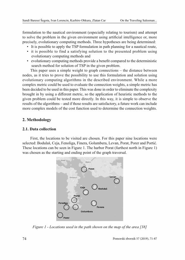
First, the locations to be visited are chosen. For this paper nine locations were selected: Bodulaš, Ceja, Fenoliga, Finera, Golumbera, Levan, Porat, Porer and Portić. These locations can be seen in Figure 1. The harbor Porat (furthest north in Figure 1) was chosen as the starting and ending point of the graph traversal.

Figure 1 - Locations used in the path shown on the map of the area [38]



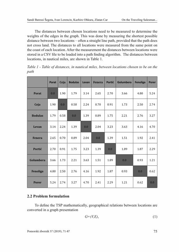
The distances between chosen locations need to be measured to determine the weights of the edges in the graph. This was done by measuring the shortest possible distance between two locations – often a straight line path, provided that the path does not cross land. The distances to all locations were measured from the same point on the coast of each location. After the measurement the distances between locations were stored in a CSV file to be loaded into a path finding algorithm. The distances between locations, in nautical miles, are shown in Table 1.

Table 1 - Table of distances, in nautical miles, between locations chosen to be on the path

Porat Ceja Bodulas Levan Fenera Portić Golumbera Fenoliga Porer

Porat 0.0 1.90 1.79 3.14 2.65 2.70 3.66 4.80 5.24

Ceja 1.90 0.0 0.58 2.24 0.70 0.91 1.73 2.50 2.74

Bodulas 1.79 0.58 0.0 1.39 0.89 1.75 2.21 2.76 3.27

Levan 3.14 2.24 1.39 0.0 2.04 3.23 3.63 4.16 4.70

Fenera 2.65 0.70 0.89 2.04 0.0 1.39 1.51 1.92 2.41

Portić 2.70 0.91 1.75 3.23 1.39 0.0 1.89 1.87 2.29

Golumbera 3.66 1.73 2.21 3.63 1.51 1.89 0.0 0.93 1.21

Fenoliga 4.80 2.50 2.76 4.16 1.92 1.87 0.93 0.0 0.62

Porer 5.24 2.74 3.27 4.70 2.41 2.29 1.21 0.62 0.0

2.2 Problem formulation

To define the TSP mathematically, geographical relations between locations are converted in a graph presentation

G=(V,E), (1)



where locations are presented with a set of vertices (V) of a graph and roads between cities are presented with a set of edges (E) [39, 40]. The graphs in TSP are usually undirected, which means that it is possible to travel in any direction between two vertices, as well as fully connected [41]. Fully connected graph means that it is possible to directly travel from any vertex in set V to any other vertex in that set by only traveling along a single edge. In other words, this means that each vertex in set V has an edge in set E connecting it directly to any other vertex in set V [42]. Edges of graph G can have weights (w(Ei)) assigned to them [39]. This is useful for such problems as the TSP, because of the cost of travel along an edge (e.g. distance). Since a problem formulation requires a fully connected graph, the distances between each and every two locations are measured. The graph used is undirected, which means that the cost of travel between two vertices is the same no matter the direction of the travel – in reality this means that the same path is taken between two locations, hence the same distance between them [43,44]. It is also important to note that the path taken between the starting and ending point is the so-called Hamiltonian cycle - a cycle within a graph that visits each vertex exactly once, before returning to the starting vertex [45].

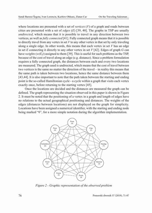
Once the locations are decided and the distances are measured the graph can be defined. The graph representing the situation observed in this paper is shown in Figure 2. It must be noted that the positioning of a vertex in a graph and length of edges have no relations to the actual geographical positioning and distances. The weights of the edges (distances between locations) are not displayed on the graph for simplicity. Locations have been assigned a numerical identifier, with the starting and ending node being marked “0”, for a more simple notation during the algorithm implementation.

Figure 2 - Graphic representation of the observed problem



To calculate paths the data need to be represented in an appropriate way. To achieve that, distances from Table 1 are stored in a two-dimensional array – with array indices being equal to the numerical identifiers of the node which enables the distance between nodes to be accessed as the array location whose indices are equal to numerical identifiers of nodes. The path is stored in a sequential linked list.

2.2. Path determination

To determine the quality of the path a fitness function needs to be determined. Fitness function is a function which determines the quality of each agent, where agent is defined as an instance of a path. In the observed case the path is determined as a sum of distances between each of the points of the path. Or, in the graph theory terminology, a sum of all weights of the edges between vertices on the path, defined per

(2)

where is the edge between vertices on indices i and i+1 in the path list.

To determine the optimal path, we can use the extensive search. Extensive search is a method that calculates the fitness function for each possible solution, i.e. for every point in the solution space. To calculate what this number is, the number of permutations possible within our paths must be calculated [46], using

(3)

where n is the number of elements in the set, and r is the size of the sample taken – the length of the path. In our case our path length is ten, but as we now that the first and last points in our path will be “0” we don’t need to include that in our calculation, making r=8. In the same manner, there are nine possibilities in total for each point in the path, but we also don’t need to include “0” as we know that the vertex will be visited as it is the starting point, making n=8 in our case. With this values known, we can calculate the total number of points in the solution space as

(4)

The extensive search will calculate the fitness function for each point and return the one with the lowest value. As this is a deterministic method, it is guaranteed that the optimal solution will be returned. Extensive search is used to determine the length of paths, the shortest and longest paths possible, as well as to determine the time it takes to search all possible solutions.



2.3. Genetic algorithm

The GA is an algorithm based on the evolution [47,48]. GA starts by generating a starting population – a group of agents. Each agent contains the solution to a problem in a representation that is favorable to the programmatic representation (so called genotype) and the value, or the means to calculate the value, of fitness function. GA is based on mechanisms of crossover and mutation [5]. Crossover is a mechanism that creates a new agent from two already existing ones picked from the population and inserts it into the population if it is better than an existing agent. Two agents picked from the population and used to generate a new one are commonly referred to as “parents”, while the resulting agent after recombination is known as “child” [49]. This mechanism that replaces current agents with better ones, allows the algorithm to search for better solutions in the solution space [49,50]. Parents are picked from the population at random, although techniques that change the random distribution of probability are often used to increase the probability of better parents (those with better value of the fitness function) to be chosen, as in theory this will lead to better children to be produced. In this paper the so called “roulette wheel” selection is used. In this type of parent selection the probability of an agent from the population being picked to become a parent is directly proportional to their fitness function, so it is more likely for a better fitting agent to produce children [50]. This algorithm is an iterative method – it repeats the used mechanisms on the current population through iterations known as generations [5].

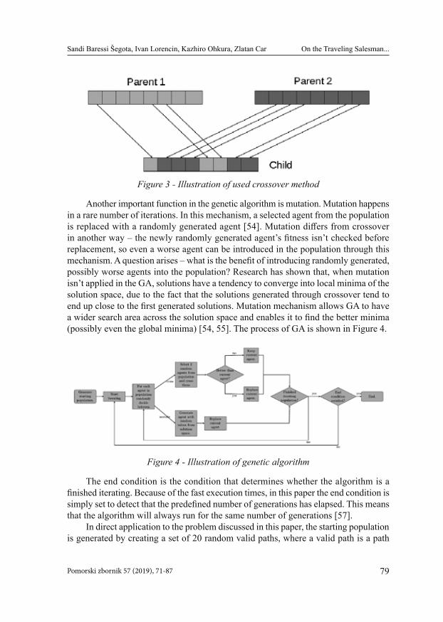
There are multiple ways a crossover can be performed between agents [52, 53]. The crossover method is usually picked to conform to the shape of the genotype. In this paper a random recombination technique has been used [52]. In this technique, a value of a child parent is randomly picked between values of two parent agents. This means that, in the observed case, a path will be constructed in a way that for each of the eight points of the path (ignoring the starting and ending point, which are both “0”) the vertex will be randomly selected from one of the chosen parents, with equal probability (i.e. a coin toss). In the observed case there is an additional constraint – a point cannot be repeated throughout the path. Consecutively, due to the length of the path being equal to the number of vertices in a graph, all vertices must be included in the path. Because of this, in the case where a point of the path that has been newly selected already exists in the path, it is to be selected from the other parent. If that point also exists in the path, then the new point of the path is randomly selected among the vertices that haven’t been chosen yet. This type of crossover is appropriate for situations where values going into a genotype are fixed and selected from a set, and cannot be calculated by using something like a mean of parents’ values.



Figure 3 - Illustration of used crossover method

Another important function in the genetic algorithm is mutation. Mutation happens in a rare number of iterations. In this mechanism, a selected agent from the population is replaced with a randomly generated agent [54]. Mutation differs from crossover in another way – the newly randomly generated agent’s fitness isn’t checked before replacement, so even a worse agent can be introduced in the population through this mechanism. A question arises – what is the benefit of introducing randomly generated, possibly worse agents into the population? Research has shown that, when mutation isn’t applied in the GA, solutions have a tendency to converge into local minima of the solution space, due to the fact that the solutions generated through crossover tend to end up close to the first generated solutions. Mutation mechanism allows GA to have a wider search area across the solution space and enables it to find the better minima (possibly even the global minima) [54, 55]. The process of GA is shown in Figure 4.

Figure 4 - Illustration of genetic algorithm

The end condition is the condition that determines whether the algorithm is a finished iterating. Because of the fast execution times, in this paper the end condition is simply set to detect that the predefined number of generations has elapsed. This means that the algorithm will always run for the same number of generations [57].

In direct application to the problem discussed in this paper, the starting population is generated by creating a set of 20 random valid paths, where a valid path is a path



in which a location is not repeated. The fitness value of each path is calculated as the length of the path. Then, the process of iterating through generations is started. In each of 50 generations a new path is generated by randomly selecting locations from each path and creating a new path, as previously described. This process is repeated for each of the existing paths. Fitness of the new path and the current existing path are compared and if the new path has a shorter length it is inserted into the generation replacing the current path. In a small number of cases (1%), due to the mutation process, a random path is generated (keeping restrictions making it valid in mind) and the current path is replaced with no regards to their lengths. With this we get multiple solutions, representing paths in the solution space. With each generation current paths are replaced with better paths moving towards a better (in this case shorter) solution. New solutions in the solution space will be located in an area between two parent paths that were used to generate them. At the end the best solution, i.e. the shortest path, is selected and presented as the final solution.

2.4. Simulated annealing

SA is an evolutionary search algorithm based on the process of the metal annealing [56]. The algorithm generates a random solution and finds its quality using a fitness function. In addition to that, a starting temperature is set. Then, the algorithm iteratively finds a neighboring solution. In our case this is performed by randomly selecting two locations in the current path and switching their places in the path. Then the fitness function of the neighboring solution is determined and if it is better than the current solution, the current solution is replaced. What differentiates this solution from a simple gradient search is the ability to select a worse solution. [58] After the neighboring solution has been generated and it has been determined that it is worse than the current solution, a new random value is generated in the range from zero to the starting system temperature [5]. If that randomly generated value is lower than the current system temperature, the current value is replaced by the worse neighboring solution. This mechanism has the same goal as the mutation mechanism in GA [5,56]. Without this mechanism applied, SA would find the local minima close to its initial, randomly selected, solution. With this mechanism applied, SA has the capability of selecting a different solution, which could lead it to find a better solution that is more distant from the initial one in the solution space. The current temperature of the system is calculated per

(5)

where Tc represents the current system temperature, Tinit the initial system temperature, k is the current iteration of the algorithm and ɑ is the cooling factor – a small value which determines how quickly the system temperature drops [5]. As the likelihood of selecting a worse agent is dependent on the system temperature, it is obvious that it



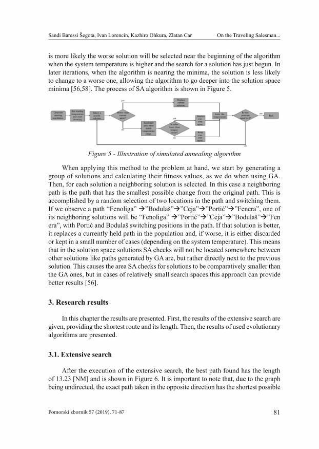
is more likely the worse solution will be selected near the beginning of the algorithm when the system temperature is higher and the search for a solution has just begun. In later iterations, when the algorithm is nearing the minima, the solution is less likely to change to a worse one, allowing the algorithm to go deeper into the solution space minima [56,58]. The process of SA algorithm is shown in Figure 5.

Figure 5 - Illustration of simulated annealing algorithm

When applying this method to the problem at hand, we start by generating a group of solutions and calculating their fitness values, as we do when using GA. Then, for each solution a neighboring solution is selected. In this case a neighboring path is the path that has the smallest possible change from the original path. This is accomplished by a random selection of two locations in the path and switching them. If we observe a path “Fenoliga” ”Bodulaš””Ceja””Portić””Fenera”, one of its neighboring solutions will be “Fenoliga” ”Portić””Ceja””Bodulaš””Fenera”, with Portić and Bodulaš switching positions in the path. If that solution is better, it replaces a currently held path in the population and, if worse, it is either discarded or kept in a small number of cases (depending on the system temperature). This means that in the solution space solutions SA checks will not be located somewhere between other solutions like paths generated by GA are, but rather directly next to the previous solution. This causes the area SA checks for solutions to be comparatively smaller than the GA ones, but in cases of relatively small search spaces this approach can provide better results [56].

3. Research results

In this chapter the results are presented. First, the results of the extensive search are given, providing the shortest route and its length. Then, the results of used evolutionary algorithms are presented.

3.1. Extensive search

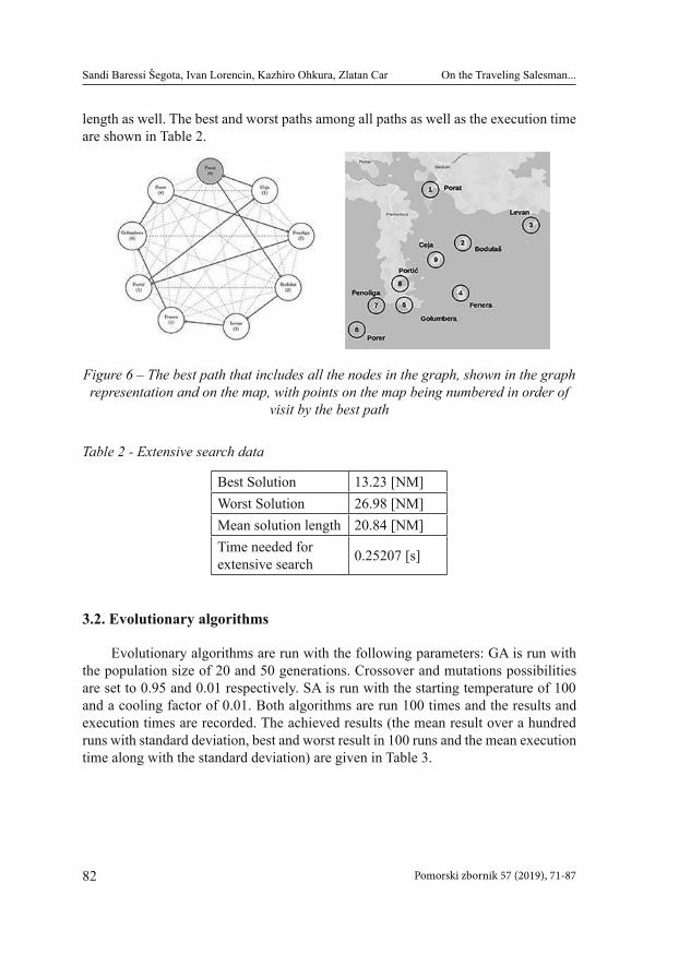
After the execution of the extensive search, the best path found has the length of 13.23 [NM] and is shown in Figure 6. It is important to note that, due to the graph being undirected, the exact path taken in the opposite direction has the shortest possible



length as well. The best and worst paths among all paths as well as the execution time are shown in Table 2.

Figure 6 – The best path that includes all the nodes in the graph, shown in the graph representation and on the map, with points on the map being numbered in order of

visit by the best path

Table 2 - Extensive search data

Best Solution 13.23 [NM]Worst Solution 26.98 [NM]Mean solution length 20.84 [NM]Time needed for extensive search 0.25207 [s]

3.2. Evolutionary algorithms

Evolutionary algorithms are run with the following parameters: GA is run with the population size of 20 and 50 generations. Crossover and mutations possibilities are set to 0.95 and 0.01 respectively. SA is run with the starting temperature of 100 and a cooling factor of 0.01. Both algorithms are run 100 times and the results and execution times are recorded. The achieved results (the mean result over a hundred runs with standard deviation, best and worst result in 100 runs and the mean execution time along with the standard deviation) are given in Table 3.



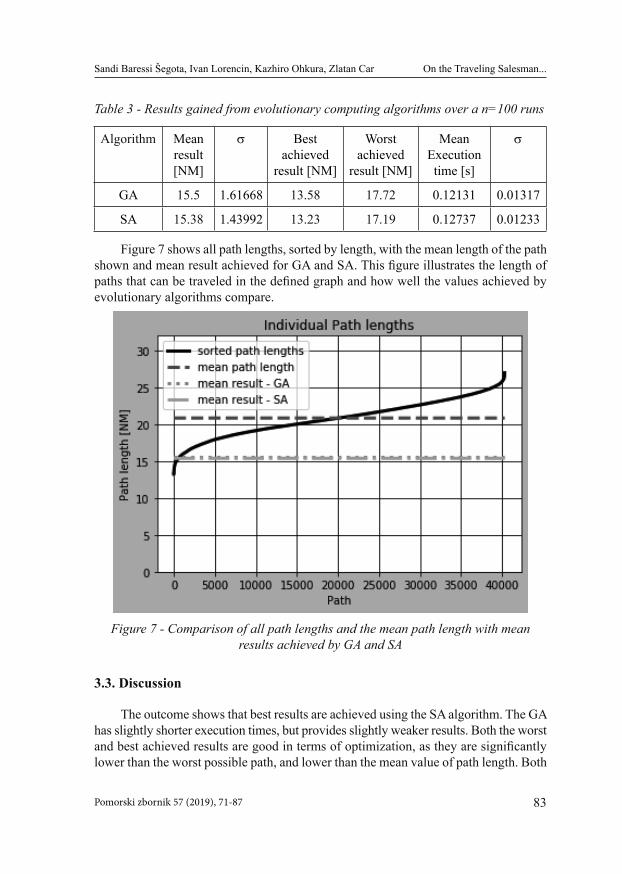
Table 3 - Results gained from evolutionary computing algorithms over a n=100 runs

Algorithm Mean result [NM]

σ Best achieved

result [NM]

Worst achieved

result [NM]

Mean Execution time [s]

σ

GA 15.5 1.61668 13.58 17.72 0.12131 0.01317

SA 15.38 1.43992 13.23 17.19 0.12737 0.01233

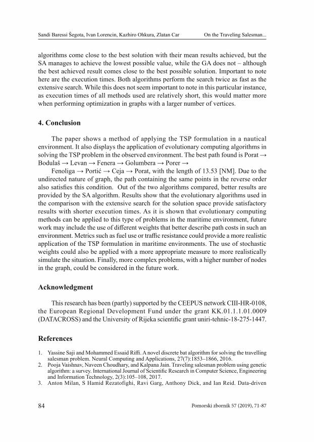
Figure 7 shows all path lengths, sorted by length, with the mean length of the path shown and mean result achieved for GA and SA. This figure illustrates the length of paths that can be traveled in the defined graph and how well the values achieved by evolutionary algorithms compare.

Figure 7 - Comparison of all path lengths and the mean path length with mean results achieved by GA and SA

3.3. Discussion

The outcome shows that best results are achieved using the SA algorithm. The GA has slightly shorter execution times, but provides slightly weaker results. Both the worst and best achieved results are good in terms of optimization, as they are significantly lower than the worst possible path, and lower than the mean value of path length. Both



algorithms come close to the best solution with their mean results achieved, but the SA manages to achieve the lowest possible value, while the GA does not – although the best achieved result comes close to the best possible solution. Important to note here are the execution times. Both algorithms perform the search twice as fast as the extensive search. While this does not seem important to note in this particular instance, as execution times of all methods used are relatively short, this would matter more when performing optimization in graphs with a larger number of vertices.

4. Conclusion

The paper shows a method of applying the TSP formulation in a nautical environment. It also displays the application of evolutionary computing algorithms in solving the TSP problem in the observed environment. The best path found is Porat → Bodulaš → Levan → Fenera → Golumbera → Porer →

Fenoliga → Portić → Ceja → Porat, with the length of 13.53 [NM]. Due to the undirected nature of graph, the path containing the same points in the reverse order also satisfies this condition. Out of the two algorithms compared, better results are provided by the SA algorithm. Results show that the evolutionary algorithms used in the comparison with the extensive search for the solution space provide satisfactory results with shorter execution times. As it is shown that evolutionary computing methods can be applied to this type of problems in the maritime environment, future work may include the use of different weights that better describe path costs in such an environment. Metrics such as fuel use or traffic resistance could provide a more realistic application of the TSP formulation in maritime environments. The use of stochastic weights could also be applied with a more appropriate measure to more realistically simulate the situation. Finally, more complex problems, with a higher number of nodes in the graph, could be considered in the future work.

Acknowledgment

This research has been (partly) supported by the CEEPUS network CIII-HR-0108, the European Regional Development Fund under the grant KK.01.1.1.01.0009 (DATACROSS) and the University of Rijeka scientific grant uniri-tehnic-18-275-1447.

References

1. Yassine Saji and Mohammed Essaid Riffi. A novel discrete bat algorithm for solving the travelling salesman problem. Neural Computing and Applications, 27(7):1853–1866, 2016.

2. Pooja Vaishnav, Naveen Choudhary, and Kalpana Jain. Traveling salesman problem using genetic algorithm: a survey. International Journal of Scientific Research in Computer Science, Engineering and Information Technology, 2(3):105–108, 2017.

3. Anton Milan, S Hamid Rezatofighi, Ravi Garg, Anthony Dick, and Ian Reid. Data-driven



approximations to np-hard problems. In Thirty-First AAAI Conference on Artificial Intelligence, 2017.

4. Paul McMenemy, Nadarajen Veerapen, Jason Adair, and Gabriela Ochoa. Rigorous performance analysis of state-of-the-art tsp heuristic solvers. In European Conference on Evolutionary Computation in Combinatorial Optimization (Part of EvoStar), pages 99–114. Springer, 2019.

5. Agoston E Eiben, James E Smith, et al. Introduction to evolutionary computing, volume 53. Springer, 2003.

6. David Hadka and Patrick Reed. Borg: An auto-adaptive many-objective evolutionary computing framework. Evolutionary computation, 21(2):231–259, 2013.

7. Yufei Wei, Motoaki Hiraga, Kazuhiro Ohkura, and Zlatan Car. Autonomous task allocation by artificial evolution for robotic swarms in complex tasks. Artificial Life and Robotics, 24(1):127–134, 2019.

8. Nikola Anđelić, Sebastijan Blažević, and Zlatan Car. Trajectory planning using genetic algorithm for three joints robot manipulator. In International Conference on Innovative Technologies, IN-TECH 2018, 2018.

9. Korino Bogović, Ivan Lorencin, Nikola Anđelić, Sebastijan Blažević, Klara Smolčić, Josip Španjol, and Zlatan Car. Artificial intelligence-based method for urinary bladder cancer diagnostic. In International Conference on Innovative Technologies, IN-TECH 2018, 2018.

10. Yufei Wei, Xiaotong Nie, Motoaki Hiraga, Kazuhiro Ohkura, and Zlatan Car. Developing end-to-end control policies for robotic swarms using deep q-learning. Journal of Advanced Computational Intelligence and Intelligent Informatics, 23(5):920–927, 2019.

11. Ivan Lorencin, Nikola Anđelić, Vedran Mrzljak, and Zlatan Car. Marine objects recognition using convolutional neural networks. NAŠE MORE: znanstveno-stručni časopis za more i pomorstvo, 66(3):112–119, 2019.

12. Lorencin, I., Anđelić, N., Španjol, J., & Car, Z. (2019). Using multi-layer perceptron with Laplacian edge detector for bladder cancer diagnosis. Artificial Intelligence in Medicine, 101746.

13. Bukovac, O., Medica, V., Mrzljak, V.: Steady state performances analysis of modern marine two-stroke low speed diesel engine using MLP neural network model, Shipbuilding: Theory and Practice of Naval Architecture, Marine Engineering and Ocean Engineering 66 (4), p. 57-70, 2015. (https://hrcak.srce.hr/149804)

14. Blažević, S., Mrzljak, V., Anđelić, N., Car, Z.: Comparison of energy flow stream and isentropic method for steam turbine energy analysis, Acta Polytechnica 59 (2), p. 109-125, 2019. (doi:10.14311/AP.2019.59.0109)

15. Lorencin, I., Anđelić, N., Mrzljak, V., Car, Z.: Exergy analysis of marine steam turbine labyrinth (gland) seals, Scientific Journal of Maritime Research 33 (1), p. 76–83, 2019. (doi:10.31217/p.33.1.8)

16. Mrzljak, V., Prpić-Oršić, J., Poljak, I.: Energy Power Losses and Efficiency of Low Power Steam Turbine for the Main Feed Water Pump Drive in the Marine Steam Propulsion System, Journal of Maritime & Transportation Sciences 54 (1), p. 37-51, 2018. (doi:10.18048/2018.54.03)

17. Poljak, I., Orović, J., Mrzljak, V.: Energy and Exergy Analysis of the Condensate Pump During Internal Leakage from the Marine Steam Propulsion System, Scientific Journal of Maritime Research 32 (2), p. 268-280, 2018. (doi:10.31217/p.32.2.12)

18. Mrzljak, V.: Low power steam turbine energy efficiency and losses during the developed power variation, Technical Journal 12 (3), p. 174-180, 2018. (doi:10.31803/tg-20180201002943)

19. Mrzljak, V., Poljak, I., Prpić-Oršić, J.: Exergy analysis of the main propulsion steam turbine from marine propulsion plant, Shipbuilding: Theory and Practice of Naval Architecture, Marine Engineering and Ocean Engineering 70 (1), p. 59-77, 2019. (doi:10.21278/brod70105)

20. Senčić, T., Mrzljak, V., Blecich, P., Bonefačić, I.: 2D CFD Simulation of Water Injection Strategies in a Large Marine Engine, Journal of Marine Science and Engineering, 7, 296, 2019. (doi:10.3390/jmse7090296)

21. Mrzljak, V., Blecich, P., Anđelić, N., & Lorencin, I. (2019). Energy and Exergy Analyses of Forced Draft Fan for Marine Steam Propulsion System during Load Change. Journal of Marine Science and Engineering, 7(11), 381.

22. Mrzljak, V., Anđelić, N., Poljak, I., Orović, J.: Thermodynamic analysis of marine steam power plant pressure reduction valves, Journal of Maritime & Transportation Sciences 56 (1), p. 9-30, 2019. (doi:10.18048/2019.56.01)



23. Mrzljak, V., Mrakovčić, T.: Comparison of COGES and Diesel-Electric Ship Propulsion Systems, Journal of Maritime & Transportation Sciences, Special edition No. 1, 2016. (doi:10.18048/2016-00.131)

24. Lorencin, I., Car, Z., Kudláček, J., Mrzljak, V., Anđelić, N., Blažević, S.: Estimation of combined cycle power plant power output using multilayer perceptron variations, 10th International Technical Conference - Technological Forum 2019 - Proceedings, Hlinsko, Czech Republic, p. 94-98, 2019.

25. Ajith Abraham and Lakhmi Jain. Evolutionary multiobjective optimization. In Evolutionary Multiobjective Optimization, pages 1–6. Springer, 2005.

26. Mrzljak, V., Orović, J., Poljak, I., Lorencin, I.: Exergy analysis of steam turbine governing valve from a super critical thermal power plant, XXVII International Scientific Conference Trans & MOTAUTO ’19 - PROCEEDINGS, Sofia, Bulgaria p. 99-102, 2019.

27. Behrendt, C., Stoyanov, R.: Operational characteristic of selected marine turbounits powered by steam from auxiliary oil-fired boilers, New Trends in Production Engineering 1 (1), p. 495-501, 2018. (doi:10.2478/ntpe-2018-0061)

28. Mrzljak, V., Žarković, B., Prpić-Oršić, J., Anđelić, N.: Numerical analysis of in-cylinder pressure and temperature change for naturally aspirated and upgraded gasoline engine, XXVII International Scientific Conference Trans & MOTAUTO ’19 - PROCEEDINGS, Sofia, Bulgaria, p. 95-98, 2019.

29. João P Trovão and Carlos Henggeler Antunes. A comparative analysis of meta-heuristic methods for power management of a dual energy storage system for electric vehicles. Energy conversion and management, 95:281–296, 2015.

30. Leonardo Antonio Monteiro Pessôa, Rodrigo Abrunhosa Collazo, Marcos Pereira Estellita Lins, Laura Bahiense, and Edilson Fernandes de Arruda. Dynamic programming applied to an oceanographic campaign planning. Revista Brasileira de Cartografia, 67(5), 2015.

31. Tomasz Neumann. The shortest path problem with uncertain information in maritime transport routing. Journal of Marine Technology & Environment, 2, 2017.

32. Mari Jevne Arnesen, Magnhild Gjestvang, Xin Wang, Kjetil Fagerholt, Kristian Thun, and Jørgen G Rakke. A traveling salesman problem with pickups and deliveries, time windows and draft limits: Case study from chemical shipping. Computers & Operations Research, 77:20–31, 2017.

33. Chunni Zhong, Chaomin Luo, Zhenzhong Chu, and Wenyang Gan. A continuous hopfield neural network based on dynamic step for the traveling salesman problem. In 2017 International Joint Conference on Neural Networks (IJCNN), pages 3318–3323. IEEE, 2017.

34. Petr Chládek and Dana Smetanová. Travelling salesman problem applied to black sea ports used by czech ocean shipping companies. NAŠE MORE: znanstveno-stručni časopis za more i pomorstvo, 65(3):141–145, 2018.

35. Aurora Smith Elgesem, Eline Sophie Skogen, Xin Wang, and Kjetil Fagerholt. A traveling salesman problem with pickups and deliveries and stochastic travel times: An application from chemical shipping. European Journal of Operational Research, 269(3):844–859, 2018.

36. Sahib Singh Juneja, Pavi Saraswat, Kshitij Singh, Jatin Sharma, Rana Majumdar, and Sunil Chowdhary. Travelling salesman problem optimization using genetic algorithm. In 2019 Amity International Conference on Artificial Intelligence (AICAI), pages 264–268. IEEE, 2019.

37. Kinjal Chaudhari and Ankit Thakkar. Travelling salesman problem: An empirical comparison between aco, pso, abc, fa and ga. In Emerging Research in Computing, Information, Communication and Applications, pages 397–405. Springer, 2019.

38. Google (n.d.) [Medulin Region] Retrieved October 15, 2019, from https://www.google.com/maps/@44.8005344,13.9349583,13z

39. Frank Harary. A seminar on graph theory. Courier Dover Publications, 2015.40. Sushanta Kumar Mohanta. Common fixed points in b-metric spaces endowed with a graph.

Matematicki Vesnik, 68(2):140–154, 2016.41. Krystian Jobczyk, Piotr Wiśniewski, and Antoni Ligza. Temporal traveling salesman problem–in

a logic-and graph theory-based depiction. In International Conference on Artificial Intelligence and Soft Computing, pages 544–556. Springer, 2018.

42. Federico Perazzi, Oliver Wang, Markus Gross, and Alexander Sorkine-Hornung. Fully connected object proposals for video segmentation. In Proceedings of the IEEE international conference on computer vision, pages 3227–3234, 2015.

43. Chao Lin, Debiao He, Xinyi Huang, Muhammad Khurram Khan, and KimKwang Raymond Choo. A new transitively closed undirected graph authentication scheme for blockchain-based identity



management systems. IEEE Access, 6:28203–28212, 2018.44. Raymond S Glover. Probabilistically finding the connected components of an undirected graph,

May 24 2016. US Patent 9,348,857.45. Eric Lewin Altschuler and Timothy J Williams. A practical efficient and effective method for the

hamiltonian cycle problem that runs on a standard computer. arXiv preprint arXiv:1701.03136, 2017.

46. Florian Pausinger. On the intriguing search for good permutations. arXiv preprint arXiv:1806.05508, 2018.

47. Lorencin, I., Anđelić, N., Mrzljak, V., & Car, Z. (2019). Genetic Algorithm Approach to Design of Multi-Layer Perceptron for Combined Cycle Power Plant Electrical Power Output Estimation. Energies, 12(22), 4352.

48. Oliver Kramer. Genetic algorithm essentials, volume 679. Springer, 2017.49. Yan Jiao and Inwhee Joe. Energy-efficient resource allocation for heterogeneous cognitive radio

network based on two-tier crossover genetic algorithm. Journal of Communications and Networks, 18(1):112–122, 2016.

50. Sankar K Pal and Paul P Wang. Genetic algorithms for pattern recognition. CRC press, 2017.51. Fengrui Yu, Xueliang Fu, Honghui Li, and Gaifang Dong. Improved roulette wheel selection-based

genetic algorithm for tsp. In 2016 International Conference on Network and Information Systems for Computers (ICNISC), pages 151–154. IEEE, 2016.

52. AJ Umbarkar and PD Sheth. Crossover operators in genetic algorithms: A review. ICTACT journal on soft computing, 6(1), 2015.

53. SG Varun Kumar and R Panneerselvam. A study of crossover operators for genetic algorithms to solve vrp and its variants and new sinusoidal motion crossover operator. Int. J. Comput. Intell. Res, 13(7):1717–1733, 2017.

54. Laith Mohammad Qasim Abualigah and Essam S Hanandeh. Applying genetic algorithms to information retrieval using vector space model. International Journal of Computer Science, Engineering and Applications, 5(1):19, 2015.

55. Jiquan Wang, Okan K Ersoy, Mengying He, and Fulin Wang. Multioffspring genetic algorithm and its application to the traveling salesman problem. Applied Soft Computing, 43:415–423, 2016.

56. Majdi M Mafarja and Seyedali Mirjalili. Hybrid whale optimization algorithm with simulated annealing for feature selection. Neurocomputing, 260:302–312, 2017.

57. Busetti, F., Simulated annealing overview, World Wide Web URL www.geocities.com/francobusetti/saweb.pdf, 4., 2003

58. Sergei V Isakov, Ilia N Zintchenko, Troels F Ronnow, and Matthias Troyer. Optimised simulated annealing for Ising spin glasses. Computer Physics Communications, 192:265–271, 2015.

On the Traveling Salesman Problem in Nautical Environments ... · On the Traveling Salesman Problem...

Documents

Transcript of On the Traveling Salesman Problem in Nautical Environments ... · On the Traveling Salesman Problem...