On the time decay of solutions in porous-elasticity with quasi-static microvoids

J. Math. Anal. Appl. 331 (2007) 617–630

www.elsevier.com/locate/jmaa

On the time decay of solutions in porous-elasticitywith quasi-static microvoids ✩

Antonio Magaña ∗, Ramón Quintanilla

Departamento Matemática Aplicada 2, UPC, C. Colón 11, 08222 Terrassa, Barcelona, Spain

Received 4 July 2006

Available online 4 October 2006

Submitted by Steven G. Krantz

Abstract

In this paper we investigate the temporal asymptotic behavior of the solutions of the one-dimensionalporous-elasticity problem with porous dissipation when the motion of microvoids is assumed to be quasi-static. This question has been recently studied in the general dynamical case. Thus, the natural question isto know if the assumption of quasi-static motion for the microvoids implies significant differences in thebehavior of the solutions from the results obtained in the general dynamical case. It is worth noting thatthis assumption involves a qualitative change in the system of equations to be analyzed because it arisesfrom the combination of a parabolic equation with an hyperbolic one, rather different from the well-knownsystem of the thermo-elastic problem. First, we study the coupling of elasticity with porosity and we showthat if only porous dissipation is present, the decay of solutions is slow, but if viscoelasticity is added, thenthe solutions decay exponentially. After that, we introduce thermal effects in the system and we show thatwhile temperature brings exponential stability to the solutions, microtemperature does not.© 2006 Elsevier Inc. All rights reserved.

Keywords: Porous-viscoelasticity; Quasi-static microvoids; Exponential stability; Energy methods; Semigroup ofcontractions

✩ This research has been partially supported by projects “Methods and models of game theory for technological andsocial sciences” and “Aspects of Stability in Thermomechanics,” Grants BFM 2003-01314 and BFM/FEDER 2003-00309, respectively, of the Science and Technology Spanish Ministry and the European Regional Development Fund.

* Corresponding author. Fax +34 93 7398101.E-mail address: [email protected] (A. Magaña).

0022-247X/$ – see front matter © 2006 Elsevier Inc. All rights reserved.doi:10.1016/j.jmaa.2006.08.086

618 A. Magaña, R. Quintanilla / J. Math. Anal. Appl. 331 (2007) 617–630

1. Introduction and preliminaries

Elasticity problems have attracted the attention of researchers from different fields interestedin the temporal decay behavior of the solutions. This interest has given many results that canbe found in the literature. In the one-dimensional case, for instance, it is known that combiningthe equations of elasticity with thermal effects provokes that a negative exponential controls thesolutions decay [15,22–24].

If elastic solids with voids are considered, as in this paper, one should look into the theoryof porous-elastic materials. Here we deal with the theory established by Cowin and Nunziato[4,5,20]. In their setting, the bulk density is the product of two scalar fields, the matrix materialdensity and the volume fraction field. It is deeply discussed in the book of Iesan [13]. We wantalso cite the recent contributions of Chirita et al. [3] and Muñoz-Rivera and Quintanilla [19].

In 1969, Grot [10] developed a theory of thermodynamics for elastic materials with mi-crostructure whose microelements, in addition to microdeformations, possess microtempera-tures. It is based on the continuum theories with microstructure, where the microelements un-dergo homogeneous deformations called microdeformations. It was extensively developed byEringen [6–9], but we also want to recall contributions [12] and [14].

The analysis of the temporal decay in one-dimensional porous-elastic materials was first stud-ied by Quintanilla [21]. The author showed that porous viscosity was not powerful enough to ob-tain exponential stability in the solutions. For the sake of completeness we recall that the solutionsgenerated by a semigroup U(t) are said to be exponentially stable if there exist two constants (in-dependent of the initial conditions) C > 0 and � > 0 such that ‖U(t)‖ � C exp(−�t)‖U(0)‖.

Through the paper, to simplify our expressions, we speak several times about slow decay or ex-ponential decay of the solutions. We will say that the decay of the solutions is exponential if theyare exponentially stable and, if they are not, we will say that the decay of the solutions is slow.Perhaps it is worth recalling the main difference between these two concepts in a thermomechan-ical context. If the decay is exponential, then after a short period of time, the thermomechanicaldisplacements are very small and can be neglected. However, if the decay is slow, then the solu-tions weaken in a way that thermomechanical displacements could be appreciated in the systemafter some time. Therefore, the nature of the solutions highly determines the temporal behaviorof the system and, from a thermomechanical point of view, it is relevant to be able to classifythem.

In a series of recent papers [1,2,18] the authors have clarified the kind of decay when wecombine temperature, elastic viscosity, porous viscosity and microtemperature. We recall themain conclusions with the help of a scheme:

If we take simultaneously one effect from the right square and other one from the left square,then we get exponential stability. However, if we consider two simultaneous effects from onesquare only, then we get slow decay. Of course, if more than two of these mechanisms are taken,we have exponential stability.

Thus, a natural question arises: will the behavior of the solutions remain unaltered if the usualequation of porosity with porous damping is replaced by the equation that corresponds to thequasi-static situation? We think that this question deserves interest from both the mechanical and

A. Magaña, R. Quintanilla / J. Math. Anal. Appl. 331 (2007) 617–630 619

mathematical points of view. From the mathematical side it is interesting because the coupling ofthe elasticity equation with the quasi-static porous equation is a mixture of a parabolic equationwith an hyperbolic equation, which is rather different from the well-known system of equationsof porous-elasticity. Furthermore, the parabolic/hyperbolic problem can be seen as the limitingcase of the hyperbolic/hyperbolic system. We will prove that the solutions of the limiting systemhave the same behavior as the elements of the sequence.

The theory of elastic solids with voids was introduced by Nunziato and Cowin [20]. Iesan[11–13] added temperature and also microtemperatures to this theory. Let us make a short pre-sentation of the general three-dimensional theory. The evolution equations are:⎧⎪⎪⎨

⎪⎪⎩ρui = tj i,j ,

J φ = hi,i + g,

ρT0η = qi,i ,

ρEi = Pji,j + qi − Qi,

where tj i is the stress tensor, hi is the equilibrated stress vector, g is the equilibrated body force,qi is the heat flux vector, η is the entropy, Pji is the first heat flux moment tensor, Qi is the meanheat flux vector, Ei is the first moment of energy vector and T0 is the absolute temperature in thereference configuration. The variables ui and φ are, respectively, the displacement of the solidelastic material and the volume fraction. We usually assume that ρ and J are positive constantswhose mechanical meaning is well known, but if quasi-static microvoids motion is considered,then we can suppose that J = 0.

To state the field equations, we need first the constitutive equations. In the general case ofsolids with viscoelasticity, porous viscosity, temperature and microtemperature we assume thefollowing (see [12,13]):⎧⎪⎪⎪⎪⎪⎪⎪⎪⎪⎨

⎪⎪⎪⎪⎪⎪⎪⎪⎪⎩

tij = λerrδij + 2μeij + bφδij + λ∗err δij + 2μ∗eij − βθδij ,

hi = δφ,i − dwi,

g = −berr + mθ − ξφ − τ φ,

ρη = βerr + cθ + mφ,

qi = kθ,i + κ1wi,

Pij = −κ4wr,rδi,j − κ5wi,j − κ6wj,i ,

Qi = (κ1 − κ2)wi + (k − κ3)θ,i ,

ρEi = −αwi − dφ,i .

Here λ, μ, b, λ∗, μ∗, β , δ, d , m, ξ , τ , c, k, κi (i = 1, . . . ,6) and α are the constitutivecoefficients, and θ and wi are the temperature and microtemperatures, respectively.

From Cowin and Nunziato [4], the constitutive coefficients for isotropic bodies satisfy thefollowing inequalities:

μ > 0, α > 0, ξ > 0, 2μ + 3λ > 0, (2μ + 3λ)ξ > 3b2. (1.1)

The other coefficients must satisfy the Clausius–Duhem conditions (see [12]).As we are considering here the one-dimensional theory and the quasi-static problem for the

microvoids motion, the evolution equations become easier and are given by⎧⎪⎪⎨⎪⎪⎩

ρu = tx,

0 = hx + g,

ρη = q∗x ,

ρE = Px + q − Q,

where q∗ stands for T −1q .
0


And the constitutive equations:⎧⎪⎪⎪⎪⎪⎪⎪⎪⎪⎨⎪⎪⎪⎪⎪⎪⎪⎪⎪⎩

t = μux + bφ + γ ux − βθ,

h = δφx − dw,

g = −bux − ξφ + mθ − τ φ,

ρη = βux + cθ + mφ,

q = kθx + κw,

P = −κ4wx,

Q = (κ∗

1 T0 − κ2)w + (

k∗T0 − κ3)θx,

ρE = −αw − dφx,

where, abusing a little bit the notation, we write μ instead of λ + 2μ and γ instead of λ∗ + 2μ∗.We also use κ∗

1 and k∗ to denote T −10 κ1 and T −1

0 k, respectively, but in the sequel, we will omitthe stars.

Thus, the constitutive coefficients, in the one-dimensional case and with the new notation,satisfy the following inequalities:

α > 0, ξ > 0, δ > 0, μξ > b2. (1.2)

In this paper it is assumed that the internal mechanical energy density is a positive definiteform. If thermal coupling is considered, b must be different from 0, but its sign does not matterin the analysis.

When thermal effects are considered, we assume that the thermal capacity c and the thermalconductivity k are strictly positive. Analogously, if microtemperatures are present, parameters α,κ4 and κ2 are positive.

Note that γ is nonnegative and we always assume that τ is strictly positive. If γ > 0 viscoelas-tic dissipation is assumed in the system.

We would like to say that we do not know any reference with an explicit formulation of theequations for porous-elastic materials with microtemperatures. Nevertheless, it is known that inthe one-dimensional linear theory, the equations that describe porosity and microstretch coincide.Therefore, we think it is appropriate to use the equations proposed by Iesan [12] to describe thistheory.

In this paper we analyze four problems. All of them are particular cases of the above system.However, it is worth noting that we do not consider in any place the complete system. In fact ouraim is to know when the solutions decay can be controlled by a negative exponential, or in otherwords, we want to know when the solutions are exponentially stable.

The boundary conditions used in this work pretend to ease the analysis carried out. To provethe slow decay we use spectral arguments, and to show the exponential decay we make useof energy methods and functional analysis. It is important to note that the spectral argumentsstrongly depend on the boundary conditions. Alternative boundary conditions do not allow to usethe same arguments. However, the method we use to prove exponential decay can be extendedwithout difficulties to other boundary conditions. This is also true for the energy method.

The paper is structured as follows. In Section 2 we study the porous-elastic problem withquasi-static microvoids when the elastic dissipation is present in the system or it is not. In Sec-tion 3 we analyze first the effect in the solutions of introducing microtemperature in the system,and second we combine elasticity, porosity and temperature. Finally, in Section 4 we summarizethe results we have obtained and some conclusions are listed. It is worth mentioning that in Sec-tion 3 we adapt to our situations the semigroup arguments, following the guidelines used in [16],that have shown to be a powerful tool to study this kind of problems.


2. Elasticity and porosity

In this section we analyze the interaction between elasticity and porosity when the elasticdissipation is present in the system or it is not. In both cases we consider viscoporosity andquasi-static microvoids, which means τ > 0 and φ ≈ 0.

Let us begin with the easier case. We assume that there is not elastic dissipation. We recallthat in the dynamical situation (φ �= 0), the solutions of the corresponding system decay in aslow way. We will see here that the same temporal behavior is obtained for the solutions of thequasi-static situation.

With the above assumptions, the system we want to study is the following{ρu = μuxx + bφx,

τ φ = δφxx − bux − ξφ,(2.1)

where τ > 0.To have the problem determined, we impose boundary and initial conditions. Thus, we assume

that the solutions satisfy the boundary conditions

u(0, t) = u(π, t) = φx(0, t) = φx(π, t) = 0, (2.2)

and the initial conditions

u(x,0) = u0(x), u(x,0) = v0(x), φ(x,0) = φ0(x). (2.3)

There are solutions uniform in the variable x. To avoid these cases, we will assume thatπ∫

0

φ0(x) dx = 0.

The spatial behavior of the solutions of this system has been recently studied in the three-dimensional case [17].

Theorem 2.1. Let (u,φ) be a solution of the problem determined by (2.1)–(2.3). Then (u,φ)

decays in a slow way.

Proof. We will prove that there exists a solution of system (2.1) of the form

u = K1eωt sin(nx), φ = K2e

ωt cos(nx),

such that Re(ω) > −ε for all positive ε. Hence, if ω is located as near as desired to the imag-inary axis, it is impossible to have uniform exponential decay on the solutions of the problemdetermined by (2.1)–(2.3).

Imposing that u and φ are as above and replacing them in (2.1) the following homogeneoussystem in the unknowns K1 and K2 is obtained:(

ρω2 + n2μ bn

bn τω + n2δ + ξ

)(K1K2

)=

(00

).

This system will have nontrivial solutions if, and only if, the determinant of the coefficientsmatrix is equal to zero. We denote by p(x) the determinant of the coefficient matrix once ω isreplaced by x:

p(x) = ρτx3 + (n2δρ + ξρ

)x2 + n2μτx + n4δμ + n2μξ − b2n2.


Notice that p(x) is a third degree polynomial and, hence, its roots can be computed by formula.Nevertheless, the expressions of the roots we have obtained using Mathematica do not let usdecide whether their real parts are negative or not. To prove that p(x) has roots as near as wewant to the complex axis, we will show that for any ε > 0 there are roots of p(x) located on theright side of the vertical line Re(z) = −ε. This fact will be shown if the polynomial p(x − ε) hasa root with positive real part. To prove that, we use the Routh–Hurwitz theorem. It asserts that, ifa0 > 0, then all the roots of polynomial

a0x3 + a1x

2 + a2x + a3

have negative real part if, and only if, all the leading minors of matrix(a1 a0 0a3 a2 a10 0 a3

)

are positive. We denote by Li , for i = 1,2,3, the leading minors of this matrix.Direct computations show that the second leading minor, L2, is a four degree polynomial on n

with negative main coefficient:

L2 = −2n4δ2ερ2 + (b2ρτ − 4δεξρ2 + 8δε2ρ2τ − 2εμρτ 2)n2 − 2εξ2ρ2 + 8ε2ξρ2τ

− 8ε3ρ2τ 2.

Thus, for n large enough, L2 is negative and p(x − ε) has a root with positive real part. (Wehave used Mathematica to compute L2.)

This argument shows that the solutions of system (2.1) decay in a slowly way, or, in otherwords, that a uniform rate of decay of exponential type for all the solutions cannot be ob-tained. �

We suppose now that our system has both porous and elastic dissipation. We will prove thatthen the solutions are exponentially stable, as they were for the dynamical case. We use here theenergy method.

The system we want to study is{ρu = μuxx + bφx + γ uxx,

τ φ = δφxx − bux − ξφ,(2.4)

where γ, τ > 0.The boundary and initial conditions are given by (2.2) and (2.3), respectively.

Theorem 2.2. Let (u,φ) be a solution of the problem determined by (2.4), (2.2) and (2.3). Then(u,φ) decays exponentially.

Proof. The energy of the system is given by

E(t) = 1

2

π∫0

(ρu2 + μu2

x + δφ2x + ξφ2 + 2buxφ

)dx.

Taking the derivative of E(t) we obtain:

E′(t) = −π∫ (

γ u2x + τ φ2)dx � −γ

π∫u2

x dx. (2.5)

0 0


Let us consider two new functions:

N1(t) =π∫

0

(ρuu + γ

2u2

x

)dx,

N2(t) = 1

2

π∫0

τφ2 dx.

We take ε > 0 small enough to make the function

I (t) = E(t) + ε(N1(t) + N2(t)

)to be equivalent to E(t).

Making the derivatives of N1(t) and N2(t) we get

N ′1(t) = −μ

π∫0

u2x dx + ρ

π∫0

u2 dx − b

π∫0

uxφ dx,

N ′2(t) = −ξ

π∫0

φ2 dx − δ

π∫0

φ2x dx − b

π∫0

uxφ dx.

Adding N ′1(t) and N ′

2(t) we obtain

N ′1(t) + N ′

2(t) = ρ

π∫0

u2 dx −π∫

0

(μu2

x + 2buxφ + ξφ2)dx −π∫

0

δφ2x dx.

And hence

I ′(t) � −γ

π∫0

u2x dx − εδ

π∫0

φ2x dx − ε

π∫0

(μu2

x + 2buxφ + ξφ2)dx + ερ

π∫0

u2 dx.

Taking into account that μξ > b2, using the Poincaré inequality and assuming that ε is smallenough, we can find a positive constant K1 such that

I ′(t) � −K1

( π∫0

u2x dx +

π∫0

φ2x dx +

π∫0

u2x dx

),

and then, we have I ′(t) � −K2I (t), with K2 > 0. That means that I (t) decays in an ex-ponential way, and so does E(t), i.e. there exist two positive constants C and � such thatE(t) � C exp(−�t)E(0). �

The arguments we have used here can be extended to other boundary conditions.

Remark 2.3. It is also possible to extend the previous arguments to the three-dimensional prob-lem, even to the case where the energy is not linear although the dissipation is. In this case thesystem is


ρui =(

∂W

∂ui,j

),j

+ aijkl uk,lj ,

τ φ =(

∂W

∂φ,k

),k

− ∂W

∂φ,

where W = W(ui,j , φ,k, φ) is such that

W � C1(ui,j ui,j + φ,kφ,k + φ2)

and

aijklui,j uk,l � C2ui,j ui,j .

C1,C2 and τ are positive and aijkl = aklij .If we define

E(t) = 1

2

∫B

(ρui ui + W)dV

and

N(t) = 1

2

∫B

(aijklui,j uk,l + 2ρuiui + τφ2)dV,

we get

E(t) = −∫B

(aijkl ui,j uk,l + τ φ2)dV

and

N(t) = −∫B

(∂W

∂ui,j

ui,j + ∂W

∂φ,k

φ,k + ∂W

∂φφ

)dV +

∫B

ρui ui dV .

If we assume that

K2W � ∂W

∂ui,j

ui,j + ∂W

∂φ,k

φ,k + ∂W

∂φφ � K1W,

where K1 and K2 are both positive, then the arguments that we have followed in the proof ofTheorem 2.2 can be applied.

3. Elasticity, porosity and thermal effects

We introduce now thermal effects in the system and do not allow elastic dissipation. First weanalyze how the presence of microtemperatures influences the behavior of the solutions, whichin the general dynamical case were proved to decay in a slow way.

For the quasi-static microvoids deformations with porous dissipation and microtemperatures,the system we should analyze is the following{

ρu = μuxx + bφx,

τ φ = δφxx − bux − ξφ − dwx,˙(3.1)

αw = κ4wxx − dφx − κ2w.


To have a well-posed problem we impose the boundary conditions

u(0, t) = u(π, t) = φx(0, t) = φx(π, t) = w(0, t) = w(π, t) = 0 (3.2)

and the initial conditions

u(x,0) = u0(x), u(x,0) = v0(x), φ(x,0) = φ0(x), w(x,0) = w0(x). (3.3)

As in Section 2, we assume thatπ∫

0

φ0(x) dx = 0.

Theorem 3.1. Let (u,φ,w) be a solution of the problem determined by (3.1)–(3.3). Then(u,φ,w) decays in a slow way.

Proof. We proceed as in the proof of Theorem 2.1. We will prove the existence of a solution ofsystem (3.1) of the form

u = K1eωt sin(nx), φ = K2e

ωt cos(nx), w = K3eωt sin(nx).

Replacing them in system (3.1) and simplifying we obtain the following homogeneous linearsystem in the unknowns K1, K2 and K3:(

n2μ + ρω2 bn 0bn n2δ + τω + ξ dn

0 −dnω αω + κ2 + κ4n2

)(K1K2K3

)=

(000

).

We denote by q(x) the determinant of the above matrix after replacing ω by x. Direct calcu-lation shows that q(x) is a fourth degree polynomial:

q(x) = αρτx4 + (d2n2ρ + n2αδρ + αξρ + κ2ρτ + n2κ4ρτ

)x3

+ (n2δκ2ρ + n4δκ4ρ + κ2ξρ + n2κ4ξρ + n2αμτ

)x2

+ (d2n4μ − b2n2α + n4αδμ + n2αμξ + n2κ2μτ + n4κ4μτ

)x

+ n6δκ4μ − b2n2κ2 − b2n4κ4 + n4δκ2μ + n2κ2μξ + n4κ4μξ.

We consider q(x − ε) and study the sign of its roots. Applying the Routh–Hurwitz theoremagain we see that the third leading minor of the corresponding matrix is a tenth degree polynomialon n with negative main coefficient for ε small enough. Let N3 be this minor, then

N3 = −2δ2εκ24 ρ3(d2 + αδ + κ4τ

)n10 + T (n),

where T (n) is an eighth degree polynomial on n. �Let us replace microtemperatures by temperature. In the general dynamical case, it is known

that the solutions decay exponentially. We will see here that this is also true for the case ofquasi-static microvoids.

The system we want to analyze is⎧⎪⎨⎪⎩

ρu = μuxx + bφx − βθx,

τ φ = δφxx − bux − ξφ + mθ,

cθ = kθxx − βux − m(δφxx − bux − ξφ + mθ).

(3.4)

τ


In this case the boundary conditions are given by

u(0, t) = u(π, t) = φx(0, t) = φx(π, t) = θx(0, t) = θx(π, t) = 0 (3.5)

and the initial conditions are

u(x,0) = u0(x), u(x,0) = v0(x), φ(x,0) = φ0(x), θ(x,0) = θ0(x). (3.6)

We denote v = u and D = ddx

, and we consider the Hilbert space

H ={

(u, v,φ, θ) ∈ H 10 × L2 × H 1 × L2,

π∫0

φ(x)dx =π∫

0

θ(x) dx = 0

}.

Then system (3.4) can be rewritten as⎧⎪⎪⎪⎪⎪⎪⎪⎪⎨⎪⎪⎪⎪⎪⎪⎪⎪⎩

u = v,

v = 1

ρ

[μD2u + bDφ − βDθ

],

φ = 1

τ

[δD2φ − bDu − ξφ + mθ

],

θ = 1

c

[kD2θ − βDv − m

τ

(δD2φ − bDu − ξφ + mθ

)].

(3.7)

If U = (u, v,φ, θ), then our initial-boundary value problem can be written as

U = AU, U0 = (u0, v0, φ0, θ0),

where A is the following 4 × 4 matrix:

A =

⎛⎜⎜⎜⎜⎝

0 I 0 0μρD2 0 b

ρD −β

ρD

− bτD 0 δD2−ξ

τmτ

mbcτ

D −βcD

m(ξ−δD2)cτ

kτD2−m2

cτ

⎞⎟⎟⎟⎟⎠ ,

where I is the identity operator.To show the exponential stability we use a result due to Gearhart (see [16]) which states that

a semigroup of contractions on a Hilbert space is exponentially stable if and only if

{iλ,λ is real} is contained in the resolvent of A, (3.8)

and

lim|λ|→∞∥∥(iλI −A)−1

∥∥ < ∞, (3.9)

where I denotes the identity matrix.We define the following inner product in H: if U∗ = (u∗, v∗, φ∗, θ∗), then

〈U,U∗〉 =π∫

0

(ρvv∗ + cθθ∗ + μuxu

∗x + δφxφ

∗x + ξφφ∗ + b

(uxφ

∗ + u∗xφ

))dx. (3.10)

Direct calculation gives

Re〈AU,U 〉 = −π∫

0

(k|θx |2 + τ−1|δφxx − bux − ξφ + mθ |2)dx � 0. (3.11)


Lemma 3.2. Let A be the above defined matrix. Then, 0 is in the resolvent of A.

Proof. For any F = (f1, f2, f3, f4) ∈H we will find U ∈H such that AU = F , or equivalently:

v = f1,

μD2u + bDφ − βDθ = ρf2,

δD2φ − bDu − ξφ + mθ = τf3,

kD2θ − βDv − m

τ

(δD2φ − bDu − ξφ + mθ

) = cf4.

⎫⎪⎪⎪⎪⎪⎬⎪⎪⎪⎪⎪⎭

(3.12)

From equation four we get

kD2θ = cf4 + βDf1 + mf3,

which can be solved. Thus we obtain θ .Then, the system reduces to

μD2u + bDφ = ρf2 + βDθ,

δD2φ − bDu − ξφ = τf3 − mθ.

}(3.13)

To show the solvability of system (3.13) we point out that

(ρf2 + βDθ, τf3 − mθ) ∈ L2 × L2.

Integrating μD2u + bDφ with respect to x we have μDu + bφ = f ∗ ∈ L2. Notice that f ∗can be univocally determined integrating with respect to x from 0 to π .

If we replace in the second equation of (3.13) Du by f ∗−bφμ

we get δD2φ − (ξ − b2

μ)φ =

g∗ ∈ L2, where g∗ can be easily obtained. As ξμ − b2 > 0, this equation has a unique solutionφ ∈ H 2 (see [25]). Then, we can also obtain a solution u to the equation

μD2u + bDφ = ρf2 + βDθ.

Consequently, system (3.12) has a solution in the domain of A. �It is also clear from the regularity theory of linear elliptic systems that

‖U‖H � K‖F‖H,

where K is a constant independent of U .

Lemma 3.3. Let A be the same matrix as in Lemma 3.2. Then condition (3.8) is satisfied.

Proof. We split the proof in three steps.(i) Since 0 is in the resolvent of A, by the contraction mapping theorem, for any real λ such

that |λ| < ‖A−1‖−1, the operator iλI − A = A(iλA−1 − I) is invertible. Moreover, ‖(iλI −A)−1‖ is a continuous function of λ in the interval (−‖A−1‖−1,‖A−1‖−1).

(ii) If sup{‖(iλI − A)−1‖, |λ| < ‖A−1‖−1} = M < ∞, then, using the contraction theoremagain, the operator

iλI −A = (iλ0I −A)(I + i(λ − λ0)(iλ0I −A)−1)

is invertible for |λ−λ0| < M−1. Hence, choosing λ0 close enough to ‖A−1‖−1, the set {λ, |λ| <‖A−1‖−1 +M−1} is contained in the resolvent of A and ‖(iλI −A)−1‖ is a continuous functionof λ in the interval (−‖A−1‖−1 − M−1,‖A−1‖−1 + M−1).


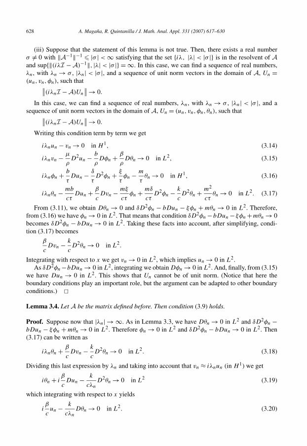
(iii) Suppose that the statement of this lemma is not true. Then, there exists a real numberσ �= 0 with ‖A−1‖−1 � |σ | < ∞ satisfying that the set {iλ, |λ| < |σ |} is in the resolvent of Aand sup{‖(iλI − A)−1‖, |λ| < |σ |} = ∞. In this case, we can find a sequence of real numbers,λn, with λn → σ , |λn| < |σ |, and a sequence of unit norm vectors in the domain of A, Un =(un, vn,φn), such that∥∥(iλnI −A)Un

∥∥ → 0.

In this case, we can find a sequence of real numbers, λn, with λn → σ , |λn| < |σ |, and asequence of unit norm vectors in the domain of A, Un = (un, vn,φn, θn), such that∥∥(iλnI −A)Un

∥∥ → 0.

Writing this condition term by term we get

iλnun − vn → 0 in H 1, (3.14)

iλnvn − μ

ρD2un − b

ρDφn + β

ρDθn → 0 in L2, (3.15)

iλnφn + b

τDun − δ

τD2φn + ξ

τφn − m

τθn → 0 in H 1, (3.16)

iλnθn − mb

cτDun + β

cDvn − mξ

cτφn + mδ

cτD2φn − k

cD2θn + m2

cτθn → 0 in L2. (3.17)

From (3.11), we obtain Dθn → 0 and δD2φn − bDun − ξφn + mθn → 0 in L2. Therefore,from (3.16) we have φn → 0 in L2. That means that condition δD2φn −bDun − ξφn +mθn → 0becomes δD2φn − bDun → 0 in L2. Taking these facts into account, after simplifying, condi-tion (3.17) becomes

β

cDvn − k

cD2θn → 0 in L2.

Integrating with respect to x we get vn → 0 in L2, which implies un → 0 in L2.As δD2φn −bDun → 0 in L2, integrating we obtain Dφn → 0 in L2. And, finally, from (3.15)

we have Dun → 0 in L2. This shows that Un cannot be of unit norm. (Notice that here theboundary conditions play an important role, but the argument can be adapted to other boundaryconditions.) �Lemma 3.4. Let A be the matrix defined before. Then condition (3.9) holds.

Proof. Suppose now that |λn| → ∞. As in Lemma 3.3, we have Dθn → 0 in L2 and δD2φn −bDun − ξφn + mθn → 0 in L2. Therefore φn → 0 in L2 and δD2φn − bDun → 0 in L2. Then(3.17) can be written as

iλnθn + β

cDvn − k

cD2θn → 0 in L2. (3.18)

Dividing this last expression by λn and taking into account that vn ≈ iλnun (in H 1) we get

iθn + iβ

cDun − k

cλn

D2θn → 0 in L2 (3.19)

which integrating with respect to x yields

iβ

un − kDθn → 0 in L2. (3.20)

c cλn


This implies un → 0 in L2. Therefore, vn → 0 in L2, too. And integrating δD2φn − bDun → 0we obtain Dφn → 0 in L2. Finally, multiplying (3.15) by vn we get

iλn〈vn, vn〉 − μ

ρ

⟨D2un, vn

⟩ → 0 in L2. (3.21)

Replacing vn by iλnun, dividing by λn and integrating by parts we obtain

i‖vn‖2 − μ

ρi‖Dun‖2 → 0 in L2,

which implies Dun → 0 in L2. �Theorem 3.5. Let (u,φ, θ) be a solution of the problem determined by (3.4)–(3.6). Then (u,φ, θ)

decays exponentially.

Proof. The proof is a direct consequence of Lemmas 3.3 and 3.4. �4. Conclusions

In this paper we have analyzed the porous-elastic problem when the motion of the microvoidsis assumed to be quasi-static. First of all, we have proved that the porous dissipation does notproduce exponential decay in the solutions. Nevertheless, if the viscoelasticity and the porousdissipation are both present, then the solutions are exponentially stable.

After that, we have introduced thermal effects on the system. If only porous damping is takeninto account, microtemperature is not strong enough to produce exponential stability. However,the porous dissipation coupled with temperature does produce it.

It is worth noting that the behavior of the solutions for each case we have analyzed hereagrees with the corresponding one for the general dynamical case. Perhaps one may think thatthis was obvious, but we think it was not because the system that arises when the motion of themicrovoids are assumed to be quasi-static is quite different from the general dynamical systemof porous-elasticity. The main difference lies in the fact that the system we have analyzed hasbeen obtained combining parabolic and hyperbolic equations, which is not standard in porous-elasticity. That means that the solutions of the parabolic/hyperbolic system, which can be thoughtof as the limiting case of the hyperbolic/hyperbolic system (limit when J tends to 0), behave inthe same way as the elements of the sequence.

References

[1] P.S. Casas, R. Quintanilla, Exponential stability in thermoelasticity with microtemperatures, Internat. J. Engrg.Sci. 43 (2005) 33–47.

[2] P.S. Casas, R. Quintanilla, Exponential decay in one-dimensional porous-thermoelasticity, Mech. Res. Comm. 32(2005) 652–658.

[3] S. Chirita, M. Ciarletta, B. Straughan, Structural stability in porous elasticity, Proc. R. Soc. A Math. Phys. Eng.Sci. 462 (2073) (8 September 2006) 2593–2605.

[4] S.C. Cowin, J.W. Nunziato, Linear elastic materials with voids, J. Elasticity 13 (1983) 125–147.[5] S.C. Cowin, The viscoelastic behavior of linear elastic materials with voids, J. Elasticity 15 (1985) 185–191.[6] A.C. Eringen, Mechanics of micromorphic materials, in: H. Gortler (Ed.), Proc. 11th Congress of Appl. Mech.,

Springer, New York, 1964.[7] A.C. Eringen, Mechanics of micromorphic continua, in: E. Kroner (Ed.), Mechanics of Generalized Continua,

Springer, Berlin, 1967, pp. 18–35.


[8] A.C. Eringen, C.B. Kafadar, Polar field theories, in: A.C. Eringen (Ed.), Continuum Physics, vol. IV, AcademicPress, New York, 1976.

[9] A.C. Eringen, Microcontinuum Field Theories, Springer, Berlin, 1999.[10] R. Grot, Thermodynamics of continuum with microstructure, Internat. J. Engrg. Sci. 7 (1969) 801–814.[11] D. Iesan, A theory of thermoelastic materials with voids, Acta Mech. 60 (1986) 67–89.[12] D. Iesan, On a theory of micromorphic elastic solids with microtemperatures, J. Thermal Stresses 24 (2001) 737–

752.[13] D. Iesan, Thermoelastic Models of Continua, Springer, 2004.[14] D. Iesan, R. Quintanilla, On a theory of thermoelasticity with microtemperatures, J. Thermal Stresses 23 (2000)

199–215.[15] S. Jiang, R. Racke, Evolution Equations in Thermoelasticity, Chapman and Hall/CRC, Boca Raton, FL, 2000.[16] Z. Liu, S. Zheng, Semigroups Associated with Dissipative Systems, Chapman and Hall/CRC, Boca Raton, FL,

1999.[17] A. Magaña, R. Quintanilla, On the spatial behavior of solutions for porous elastic solids with quasi-static microvoids,

Math. Comput. Modelling 44 (2006) 710–716.[18] A. Magaña, R. Quintanilla, On the time decay of solutions in one-dimensional theories of porous materials, Internat.

J. Solids Structures 43 (2006) 3414–3427.[19] J. Muñoz-Rivera, R. Quintanilla, On the time polynomial decay in elastic solids with voids, Manuscript, 2006.[20] J.W. Nunziato, S.C. Cowin, A nonlinear theory of elastic materials with voids, Arch. Ration. Mech. Anal. 72 (1979)

175–201.[21] R. Quintanilla, Slow decay for one-dimensional porous dissipation elasticity, Appl. Math. Lett. 16 (2003) 487–491.[22] R. Quintanilla, R. Racke, Stability for thermoelasticity of type III, Discrete Contin. Dyn. Syst. Ser. B 3 (2003)

383–400.[23] R. Quintanilla, R. Racke, Qualitative aspects in dual-phase-lag thermoelasticity, SIAM J. Appl. Math. 66 (2006)

977–1001.[24] M. Slemrod, Global existence, uniqueness and asymptotic stability of classical smooth solutions in one-dimensional

nonlinear thermoelasticity, Arch. Ration. Mech. Anal. 76 (1981) 97–133.[25] R. Temam, Infinite Dimensional Dynamical Systems in Mechanics and Physics, Springer, New York, 1988.

On the time decay of solutions in porous-elasticity with quasi-static microvoids

Documents

Transcript of On the time decay of solutions in porous-elasticity with quasi-static microvoids