On the thermodynamic pre-conditioning of Arctic air masses ...
40
manuscript submitted to JGR: Atmospheres On the thermodynamic pre-conditioning of Arctic air 1 masses and the role of tropopause polar vortices for 2 cold air outbreaks from Fram Strait 3 Lukas Papritz 1 , Emmanuel Rouges 1* , Franziska Aemisegger 1 , and Heini 4 Wernli 1 5 1 Institute for Atmospheric and Climate Science, ETH Z¨ urich, Z¨ urich, Switzerland 6 Key Points: 7 • Cold air outbreak (CAO) air masses experience average radiative cooling rates but 8 reside in the Arctic for an exceptionally long time 9 • Tropopause polar vortices (TPVs) gather cold air masses in the Arctic and con- 10 tribute to intense CAOs when they approach Fram Strait 11 • The most intense CAOs are more often related to TPVs (40% of the top 40 events) 12 than weaker ones (20% of the top 60 to top 100 events) 13 * now at Swiss Federal Institute for Forest, Snow, and Landscape Research (WSL), Birmensdorf, Switzer- land Corresponding author: Lukas Papritz, [email protected] –1–
Transcript of On the thermodynamic pre-conditioning of Arctic air masses ...

manuscript submitted to JGR: Atmospheres
On the thermodynamic pre-conditioning of Arctic air1
masses and the role of tropopause polar vortices for2
cold air outbreaks from Fram Strait3
Lukas Papritz1, Emmanuel Rouges1∗, Franziska Aemisegger1, and Heini4
Wernli15
1Institute for Atmospheric and Climate Science, ETH Zurich, Zurich, Switzerland6
Key Points:7
• Cold air outbreak (CAO) air masses experience average radiative cooling rates but8
reside in the Arctic for an exceptionally long time9
• Tropopause polar vortices (TPVs) gather cold air masses in the Arctic and con-10
tribute to intense CAOs when they approach Fram Strait11
• The most intense CAOs are more often related to TPVs (40 % of the top 40 events)12
than weaker ones (20 % of the top 60 to top 100 events)13
∗now at Swiss Federal Institute for Forest, Snow, and Landscape Research (WSL), Birmensdorf, Switzer-
land
Corresponding author: Lukas Papritz, [email protected]
–1–
manuscript submitted to JGR: Atmospheres
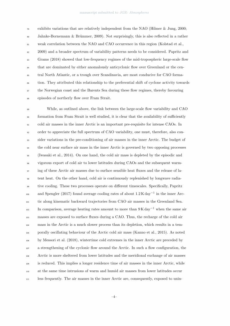
Abstract14
Fram Strait is a hot-spot of Arctic cold air outbreaks (CAOs), which typically oc-15
cur within the northerly flow associated with a strong low-tropospheric east-west pres-16
sure gradient between Svalbard and Greenland. This study investigates the processes in17
the inner Arctic that thermodynamically pre-condition air masses associated with CAOs18
south of Fram Strait where they lead to negative potential temperature anomalies of-19
ten in excess of 15 K. Kinematic backward trajectories from Fram Strait are used to quan-20
tify the Arctic residence time and to analyse the thermodynamic evolution of these air21
masses. Additionally, the study explores the importance of cyclonic tropopause polar vor-22
tices (TPVs) for CAO formation south of Fram Strait. Results from a detailed case study23
and the climatological analysis of the 100 most intense CAOs from Fram Strait in the24
ERA-Interim period reveal that: (i) air masses that cause CAOs (CAO air masses) re-25
side longer in the inner Arctic compared to those that do not (NO-CAO air masses), and26
they originate from climatologically colder regions; (ii) the 10-day accumulated cooling27
is very similar for CAO and NO-CAO air masses indicating that the transport history28
and northerly origin of the air masses is more decisive for the formation of an intense29
negative temperature anomaly south of Fram Strait than an enhanced inner-Arctic di-30
abatic cooling; (iii) 40 % (29 %) of the top 40 (100) CAOs are related to a TPV in the31
vicinity of Fram Strait; (iv) TPVs confine anomalously cold air masses within their as-32
sociated low-tropospheric cold dome leading to enhanced accumulated radiative cooling.33
1 Introduction34
Fram Strait, the passage between Greenland and Svalbard at about 80◦N, is an im-35
portant gateway for the exchange of mass and energy between the north-eastern North36
Atlantic and the inner Arctic, here defined as the basin of the Arctic Ocean (cf. Fig. 137
for location names). Especially intense meridional winds over Fram Strait lead to exchange38
processes that are of key importance for the Arctic climate system. For instance, northerly39
winds drive the export of sea ice from the Arctic basin into the Greenland Sea and the40
strength and direction of these winds account for most of the day-to-day variability of41
the ice export (Tsukernik et al., 2009; Jahnke-Bornemann & Brummer, 2009). During42
winter such northerly winds also advect very cold air masses from the inner Arctic over43
the comparatively warm waters of the Nordic Seas, giving rise to marine cold air out-44
breaks (CAOs).45
–2–
manuscript submitted to JGR: Atmospheres
Due to the temperature deficit of CAO air masses with respect to the sea surface46
temperature (SST), intense upward fluxes of sensible heat ensue (e.g., Brummer, 1997;47
Renfrew & Moore, 1999; Wacker, Jayaraman Potty, Lupkes, Hartmann, & Raschendor-48
fer, 2005). Furthermore, as a result of their initial dryness, the rapid warming by sen-49
sible heat fluxes, and the typically high wind speeds (Kolstad, 2017), CAO air masses50
pick up substantial amounts of moisture via evaporation from the ocean surface, which51
for intense and large-scale CAOs can exceed 5 % of the hemispheric water content pole-52
ward of 40◦N, and are, thus, an important element of the high latitude atmospheric wa-53
ter budget (Aemisegger & Papritz, 2018; Papritz & Sodemann, 2018). Consequently, CAO54
air masses are rapidly transformed from anomalously cold and dry into much warmer55
and moist air masses. This can lead to vigorous convective overturning and the release56
of latent heat during cloud formation (see review by Pithan et al., 2018 and references57
therein). At the same time, the surface heat fluxes cool the ocean’s mixed layer; in fact,58
CAOs deliver the bulk of the wintertime heat flux forcing of the Nordic Seas (Papritz59
& Spengler, 2017) and are the key driver for ocean convection at the northernmost ex-60
tremity of the Atlantic Meridional Overturning Circulation (Marshall & Schott, 1999;61
Buckley & Marshall, 2016). Due to their important role in the climate system, CAOs62
in the Nordic Seas have garnered increasing interest in recent years and - as we outline63
below - substantial progress has been made in terms of the mechanistic understanding64
of CAO formation in this region and the associated air mass transformations. Neverthe-65
less many facets of the drivers of CAO variability remain unexplored and require fur-66
ther investigation.67
Climatological analyses revealed that the bulk of the air masses associated with CAOs68
south of Fram Strait, namely in the Greenland and Iceland Seas, have their origin in the69
inner Arctic and are carried through Fram Strait by northerly winds (Kolstad et al., 2009;70
Papritz & Spengler, 2017). These winds are typically in near geostrophic balance and71
are, therefore, associated with higher pressure towards north-eastern Greenland and lower72
pressure towards the Svalbard Archipelago (Tsukernik et al., 2009). Consequently, the73
variability of CAO formation is to a large extent modulated by the frequency of tran-74
sient cyclones in the Nordic Seas and the Barents Sea. Since Fram Strait is located far75
north of the primary centers of action of the North Atlantic Oscillation (NAO), and be-76
cause the North Atlantic storm track features a secondary branch that extends across77
the Nordic Seas into the Barents Sea (Dacre & Gray, 2009), the flow over Fram Strait78
–3–
manuscript submitted to JGR: Atmospheres
exhibits variations that are relatively independent from the NAO (Hilmer & Jung, 2000;79
Jahnke-Bornemann & Brummer, 2009). Not surprisingly, this is also reflected in a rather80
weak correlation between the NAO and CAO occurrence in this region (Kolstad et al.,81
2009) and a broader spectrum of variability patterns needs to be considered. Papritz and82
Grams (2018) showed that low-frequency regimes of the mid-tropospheric large-scale flow83
that are dominated by either anomalously anticyclonic flow over Greenland or the cen-84
tral North Atlantic, or a trough over Scandinavia, are most conducive for CAO forma-85
tion. They attributed this relationship to the preferential shift of cyclone activity towards86
the Norwegian coast and the Barents Sea during these flow regimes, thereby favouring87
episodes of northerly flow over Fram Strait.88
While, as outlined above, the link between the large-scale flow variability and CAO89
formation from Fram Strait is well studied, it is clear that the availability of sufficiently90
cold air masses in the inner Arctic is an important pre-requisite for intense CAOs. In91
order to appreciate the full spectrum of CAO variability, one must, therefore, also con-92
sider variations in the pre-conditioning of air masses in the inner Arctic. The budget of93
the cold near surface air mass in the inner Arctic is governed by two opposing processes94
(Iwasaki et al., 2014). On one hand, the cold air mass is depleted by the episodic and95
vigorous export of cold air to lower latitudes during CAOs and the subsequent warm-96
ing of these Arctic air masses due to surface sensible heat fluxes and the release of la-97
tent heat. On the other hand, cold air is continuously replenished by longwave radia-98
tive cooling. These two processes operate on different timescales. Specifically, Papritz99
and Spengler (2017) found average cooling rates of about 1.2 K day−1 in the inner Arc-100
tic along kinematic backward trajectories from CAO air masses in the Greenland Sea.101
In comparison, average heating rates amount to more than 9 K day−1 when the same air102
masses are exposed to surface fluxes during a CAO. Thus, the recharge of the cold air103
mass in the Arctic is a much slower process than its depletion, which results in a tem-104
porally oscillating behaviour of the Arctic cold air mass (Kanno et al., 2015). As noted105
by Messori et al. (2018), wintertime cold extremes in the inner Arctic are preceded by106
a strengthening of the cyclonic flow around the Arctic. In such a flow configuration, the107
Arctic is more sheltered from lower latitudes and the meridional exchange of air masses108
is reduced. This implies a longer residence time of air masses in the inner Arctic, while109
at the same time intrusions of warm and humid air masses from lower latitudes occur110
less frequently. The air masses in the inner Arctic are, consequently, exposed to unin-111
–4–

manuscript submitted to JGR: Atmospheres
hibited radiative cooling over a prolonged period and can acquire a substantial temper-112
ature deficit with respect to climatology. If northerly winds over Fram Strait happen to113
tap such a reservoir of unusually cold air, it can be expected that the resulting CAO is114
particularly intense.115
In many cases, the accumulation and coherent transport of anomalously cold Arc-116
tic air masses that lead to intense CAOs can - as we will explore in this study - be re-117
lated to an ubiquitous type of dynamical weather system that is unique to the polar re-118
gions, so-called tropopause polar vortices (hereafter TPVs). These are subsynoptic cy-119
clonic vortices at the tropopause level with a diameter of typically 1000 to 1500 km and120
a lifetime of weeks to more than a month (Cavallo & Hakim, 2009, 2010). They are dy-121
namically characterized by a positive potential vorticity (PV) anomaly in the Arctic lower122
stratosphere, associated with a downward bending of the dynamical tropopause often123
to the 500 hPa level or below, and a dome of anomalously cold tropospheric air under-124
neath the PV anomaly and a warm anomaly aloft in the stratosphere. They are main-125
tained by differential radiative cooling between the relatively humid troposphere and the126
very dry stratosphere, which is associated with a diabatic generation of PV near the dy-127
namical tropopause and, hence, an amplification of the TPV (Cavallo & Hakim, 2013).128
When leaving the inner Arctic, TPVs can instigate the genesis of surface cyclones (Hakim,129
2000; Kew et al., 2010). In addition, if the track of the TPV leads over a warm ocean130
surface, the dome of anomalously cold tropospheric air associated with the TPV is likely131
resulting in a CAO. By gathering radiatively cooled air masses in their lower tropospheric132
core, they could also play an important role in the long-range transport of CAO air masses133
and prolonging their residence time in the inner Arctic. As yet, these potential linkages134
between CAOs from Fram Strait and TPVs have not been systematically explored. Thus,135
we hypothesise here that TPVs approaching the vicinity of Fram Strait are an impor-136
tant factor in establishing particularly intense CAOs downstream of Fram Strait.137
In this study we aim to address the following questions regarding dynamical mech-138
anisms and the thermodynamic evolution of the air masses leading to the most intense139
CAOs from Fram Strait:140
1. Does the history of air masses that cause intense CAOs share common character-141
istics such as a more intense diabatic cooling or a longer residence time in the Arc-142
tic compared to air masses that do not?143
–5–

manuscript submitted to JGR: Atmospheres
2. When do these air masses become anomalously cold relative to the time when they144
pass through Fram Strait?145
3. What is the relative importance of diabatic pre-conditioning and transport from146
climatologically colder regions towards Fram Strait for establishing the necessary147
cold anomaly?148
4. How often are TPVs involved in the export of very cold Arctic air masses and the149
formation of intense CAOs?150
We consider the 100 most intense CAOs from Fram Strait in the ERA-Interim reanal-151
ysis, make use of kinematic trajectories from Fram Strait to investigate the thermody-152
namic history of these CAO air masses, and implement a feature based identification and153
tracking of TPVs. The methodology will be outlined in Section 2, followed by the de-154
tailed case study of an exceptional sequence of CAOs associated with a long-lived TPV155
in Section 3. Section 4 is then devoted to the climatological investigation of the aformen-156
tioned questions, followed by concluding remarks in Section 5.157
2 Methodology158
We base this study on the interim reanalysis from the European Centre for Medium-159
Range Weather Forecasts (ERA-Interim; Dee et al., 2011). Fields are available in 6-hourly160
intervals on 60 model levels, and they are interpolated from the model’s spectral T255161
resolution onto a regular 1◦×1◦ longitude-latitude grid. The study period includes the162
boreal winters (Dec - Feb) 1979/80 to 2015/16. Climatological values are defined as the163
calendar-day climatology, that is the mean over all instances of a specific day of year in164
the record. For example, the calendar-day climatology for 21 January would be the mean165
of every 21 January in the record. This timeseries is then smoothed by a 10-day running166
mean filter. Thereby, the 10-day running mean provides a reasonable compromise be-167
tween the desire to retain intra-seasonal variations in the climatology and the need to168
filter out spurious fluctuations resulting from the limited length of the record. In the fol-169
lowing, we will introduce three diagnostics that we apply in order to identify principal170
flow features used for the characterisation of CAOs from Fram Strait. Specifically, these171
diagnostics comprise (1) the identification of CAO air masses and events, (2) the anal-172
ysis of transport pathways of air masses reaching Fram Strait from the North, as well173
as (3) the identification and tracking of TPVs.174
–6–

manuscript submitted to JGR: Atmospheres
2.1 Identification of CAO air masses and events175
For the identification of CAO air masses over open ocean we consider the differ-176
ence between potential sea surface temperature (θSST) and θ at the 900 hPa level (θSST−177
θ900). Positive values of this so-called CAO index indicate an air mass colder than the178
sea surface. Such air masses feature the typical characteristics of marine CAOs, namely179
upward fluxes of sensible heat, the uptake of moisture, and convective overturning with180
cloud formation and the associated release of latent heat (e.g., Brummer, 1997; Renfrew181
& Moore, 1999; Papritz, Pfahl, Sodemann, & Wernli, 2015; Papritz & Sodemann, 2018).182
This definition of CAOs has - sometimes with slight variations - been employed in a num-183
ber of previous studies of CAOs in this region (e.g., Bracegirdle & Gray, 2008; Kolstad184
& Bracegirdle, 2008; Kolstad et al., 2009; Papritz & Spengler, 2017; Knudsen et al., 2018;185
Papritz & Sodemann, 2018).186
Averaging this CAO index spatially over the region 20◦W - 14◦E and 71◦N - 81◦N187
(see purple framed box Fig. 1) and excluding grid points over land and over ocean if the188
sea ice concentration is larger than 0.5 yields the Fram Strait CAO index timeseries. We189
identify CAO events in the Greenland Sea as local maxima of this timeseries that ex-190
ceed its 90th percentile (9.34 K). Start and end dates of a CAO event are then defined191
as the timesteps closest to the first time when the CAO index exceeds or falls below the192
detection threshold. To avoid the detection of spurious CAO events due to short term193
fluctuations of the CAO index around the threshold, we treat consecutive CAO events194
as one single event if less than 20 % of the timesteps between the onset of the first event195
and the end of the second event are below the threshold and the time averaged CAO in-196
dex exceeds the threshold. Finally, we rank the CAO events according to the maximum197
of the CAO index reached during the period of each event, in the following referred to198
as the intensity of the event. This approach results in a total of 146 CAO events through-199
out the study period, from which we select the 100 most intense events for further anal-200
ysis (see Fig. 2).201
Note that the seasonal 90th percentile of the 6-hourly CAO index timeseries fea-202
tures a declining trend of −0.72 K decade−1 throughout the study period (Fig. 2), which203
is owed to the more rapid increase of the 900 hPa Arctic air temperature than the SST204
(not shown). Using a fixed threshold, therefore, may cause the detection of more events205
at the beginning of the study period than at the end. The pronounced interannual vari-206
–7–

manuscript submitted to JGR: Atmospheres
ability of the seasonal 90th percentile, however, clearly dwarves the linear trend (cf. box-207
plots in Fig. 2). Furthermore, the large amplitude of the 100 most intense events com-208
pared to the changes in the seasonal 90th percentile implies that all of the events lie out-209
side or at the edge of the confidence interval for the linear regression of the seasonal 90th210
percentile of the CAO index. Consequently, the same events were detected if the CAO211
timeseries was detrended or a threshold linearly decreasing with time was used.212
2.2 Kinematic trajectories from Fram Strait213
To investigate transport pathways and the thermodynamic evolution of air masses214
reaching Fram Strait from the inner Arctic, we compute air mass trajectories using the215
Lagrangian Analysis Tool (LAGRANTO; Sprenger & Wernli, 2015). For that purpose,216
we define for every 6 hourly timestep in the study period a set of points at 900 hPa along217
the latitude circle of 81.5◦N from 20◦W to 14◦E, that is 0.5◦ poleward of the northern218
boundary of the box used for computing the CAO index, with an equidistant horizon-219
tal spacing of 35 km, corresponding to twice the longitudinal distance between grid points220
at 81.5◦N. Among these potential trajectory starting points, we select the subset of grid221
points where the wind has a northerly component. This ensures that trajectories are only222
computed for air masses that approach Fram Strait from the North. Finally, for these223
starting points, we compute trajectories forward and backward in time for 48 h and 240 h,224
respectively, and we trace additional quantities, such as θ and the CAO index, by inter-225
polating these fields to the trajectory positions. Throughout the study we will refer to226
the initialization time of the trajectories as t = 0 h.227
2.3 Identification and tracking of TPVs228
As an additional diagnostic, we identify and track TPVs from the anomaly field229
of PV vertically averaged between 600 hPa and 200 hPa (VAPV). Specifically, we define230
VAPV anomalies as deviations from the calendar-day climatology of VAPV smoothed231
with a 10-day running mean. The procedure to obtain the TPV tracks involves four steps:232
First, we identify all local maxima of positive VAPV anomalies poleward of 60◦N and233
search for the outermost closed VAPV anomaly contours surrounding these maxima with234
a search interval of 0.1 PVU (1 PVU = 10−6 K kg−1 m2 s−1). Second, if local maxima235
occur in close proximity to each other (distance < 800 km), we keep only the largest max-236
imum for further tracking. Third, we employ the tracking algorithm by Wernli and Schwierz237
–8–
manuscript submitted to JGR: Atmospheres
(2006) with modifications by Sprenger et al. (2017) - originally developed for the track-238
ing of surface cyclones - to generate tracks of the TPVs. Fourth, we retain only tracks239
that last for at least 72 h and attain a VAPV anomaly of 1.5 PVU or more at least once240
along the track. All in all, this procedure is designed to identify well-defined intense upper-241
tropospheric, cyclonic vortices with a clearly polar origin.242
3 Case study of an episode with three cold air outbreaks243
3.1 Synoptic evolution244
In this section, we discuss an episode with a series of three consecutive CAOs that245
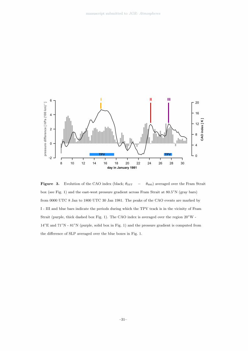
occurred in January 1981, among them the third most intense CAO in the study period.246
Figure 3 shows the evolution of the CAO index during this period, revealing three dis-247
tinct peaks, on 15, 24, and 27 January. Thereafter, we will refer to these CAO events248
as events I - III. They are ranked 3, 77, and 71 among the 100 CAO events in terms of249
intensity. A strengthening of the northerly flow precedes these peaks, as evident from250
the east-west pressure gradient across Fram Strait computed from the difference of area251
averaged SLP in the blue boxes shown in Fig. 1. This reflects the importance of the trans-252
port of cold air masses from the inner Arctic into the basin of the Greenland Sea (cf. Fig. 1)253
for inducing these CAOs (Papritz & Spengler, 2017) - yet the first and most intense CAO254
is not preceded by exceptionally strong northerly flow compared to the other two events.255
This suggests that the availability of particularly cold air masses in the inner Arctic is256
a principal factor in modulating the intensity of CAOs during northerly flow periods.257
A unique feature of this episode is the co-occurrence of two of the CAO events with258
the repeated propagation of a single, long-lived TPV out of the inner Arctic into the vicin-259
ity of Fram Strait. The periods when the TPV leaves the inner Arctic near Fram Strait260
are marked by blue horizontal bars in Fig. 3. Furthermore, the synoptic evolution of the261
episode and the track of the TPV are displayed in Figs. 4 and 5. The TPV has genesis262
north of Bering Strait on 2 Jan 1981, crosses the North Pole and then follows a cycloni-263
cally curved track, such that it remains in the inner Arctic (cf. track in Fig. 4a). At 0600264
UTC 10 Jan the TPV features a cyclonic circulation in the mid-troposphere with only265
a weak signature in surface pressure but a strong negative θ anomaly at 900 hPa well ex-266
ceeding 14 K (Figs. 4a, b). This θ anomaly is clearly linked to the dynamical structure267
of the TPV, as evident from the vertical cross section shown in Fig. 6. It reveals a deep268
–9–

manuscript submitted to JGR: Atmospheres
downward excursion of stratospheric air, characterised by PV values in excess of 2 PVU,269
with the dynamical tropopause (cf. 2 PVU surface) reaching down to about 750 hPa (Fig. 6a).270
Furthermore, it features the archetypal thermal anomalies that are associated with pos-271
itive PV anomalies (e.g., Hoskins, McIntyre, & Robertson, 1985) and a characteristic prop-272
erty of TPVs (Cavallo & Hakim, 2010), that is a cold anomaly underneath the PV anomaly273
reaching from the surface throughout the entire troposphere and a weaker warm anomaly274
aloft in the stratosphere (Fig. 6b).275
Subsequently, the TPV gradually approaches Fram Strait in conjuction with the276
dome of anomalously cold air underneath, reaching the northern edge of the CAO tar-277
get region at 1800 UTC 12 Jan (Figs. 4c, d). Within the next 2.5 days, the TPV slowly278
moves further equatorward and thus gives rise to CAO event I (cf. Figs. 3 and 4e, f). In279
this process, the strong negative θ anomaly amplifies substantially as the air masses reach280
the Greenland Sea - a climatologically much warmer region owing to the relatively warm281
ocean surface - thus, leading to the strong air-sea temperature contrast.282
Eventually, the TPV returns into the inner Arctic and by 1200 UTC 22 Jan its cen-283
ter is once more located in the vicinity of the North Pole (Fig. 5a), while it still main-284
tains a strongly anomalous cold air mass underneath (Fig. 5b). Within the next five days,285
it slowly migrates equatorward (Figs. 5c, d). Thereby, the TPV helps in establishing a286
cyclonically curved flow that extends beyond the region with anomalously cold air as-287
sociated with the TPV. This cyclonic flow leads to the transport of cold air masses from288
Siberia across the central Arctic towards Fram Strait (Figs. 5c, d). As these air masses289
approach the climatologically warmer Fram Strait, they attain a negative θ anomaly, thus290
resulting in CAO event II on 24 Jan 1981. The TPV itself, however, remains in the in-291
ner Arctic.292
During the next four days, the TPV propagates further equatorward towards Sval-293
bard and then into the Barents Sea. This gives rise to a rapid increase of the CAO in-294
dex after 0000 UTC 27 Jan, and thus, to CAO event III (Figs. 5e, f). The resulting θ295
anomaly underneath the TPV is equally strong as during CAO event I (Figs. 5d, f). Since296
the track of the TPV is displaced eastward and directed into the Barents Sea, the cold-297
est air masses are located over the Svalbard archipelago and subsequently spill into the298
Barents Sea, whereas in the Fram Strait region the θ anomaly is considerably weaker -299
–10–

manuscript submitted to JGR: Atmospheres
yet sufficient to be characterized as an intense CAO. Consequently, the CAO index does300
not reach as high values as during CAO event I (Fig. 3).301
3.2 Pathways and thermodynamic evolution of CAO air masses in the302
Arctic303
Kinematic trajectories from Fram Strait (81.5◦N) initialized in 6-hourly intervals304
from −24 h to 0 h relative to the peak of the CAO event give insight into the transport305
pathways of the CAO air masses and, in particular, their relation to the TPV. The tra-306
jectory locations at the peak times of the CAO events (dots in Fig. 7) reveal that tra-307
jectories released during this 24 h period provide a reasonable sampling of the CAO air308
mass in the CAO target box at the time of maximum intensity. Five days before the peak309
of CAO event I, the majority of the trajectories (crosses in Figure 7a) are located in the310
vicinity of the TPV irrespective of their initialization time. A second group of trajec-311
tories is located south of the TPV near the Siberian coast. They are subsequently ad-312
vected towards Fram Strait by the cyclonic flow in the periphery of the TPV, as exem-313
plified by the explicitely drawn trajectories that were initialized at the peak time of the314
CAO event. Furthermore, the colour shading indicates that all trajectories remained be-315
tween the surface and about 850 hPa throughout their evolution. The trajectories directly316
below the TPV have a tendency to descend by about 50 - 100 hPa until they reach Fram317
Strait.318
The trajectories in the vicinity of the TPV form part of the tropospheric cold dome319
underneath the TPV as evident from the cross-section (crosses in Fig. 6b). In fact, most320
of these trajectories enter the TPV’s cold dome already before 7 Jan more than 8 days321
before the peak of the CAO event (not shown). Thereafter, these trajectories move in322
collocation with the TPV. This suggests that the dynamical structure of the TPV pro-323
vides a material boundary for the anomalously cold air masses allowing for further cool-324
ing in accord with an intensification of the TPV (Cavallo & Hakim, 2013). This char-325
acteristic is in strong contrast to, for example, extratropical cyclones, where Lagrangian326
air streams continuously enter and exit the system (e.g., Browning, 1990; Wernli, 1997).327
In the case of CAO event III a larger group of trajectories reaching Fram Strait orig-328
inates from Siberia and follows a cyclonically curved pathway across the inner Arctic to-329
wards Fram Strait, while only trajectories arriving in the eastern segment of Fram Strait330
–11–

manuscript submitted to JGR: Atmospheres
are part of the TPV’s cold dome (Fig. 7b). Nevertheless, the TPV still plays a key role331
for the transport of air masses contributing to this CAO event in Fram Strait. Due to332
the TPV’s spatial extent as well as its long residence time near the pole, it gives rise to333
a near-surface long-range transport from Siberia across the inner Arctic to Fram Strait334
(cf. trajectories drawn in Fig. 7b), which is an important prerequisite for the formation335
of CAO event III. A similar long-range transport is also observed for CAO event II (not336
shown), however, with the TPV remaining in the inner Arctic.337
The key factor for the formation of an intense CAO is the existence of a strong θ338
anomaly at the time when trajectories reach Fram Strait (i.e., t = 0 h). The relative339
contributions of transport and diabatic cooling to the emergence of such a θ anomaly340
can be understood in terms of the air masses’ distinct signatures in the phase space spanned341
by θ and the climatological θ (θc; Fig. 8). Values in the lower right half of Fig. 8 indi-342
cate a negative θ anomaly. Horizontal displacements from left to right (at constant θ)343
in this phase space correspond to the creation of a negative θ anomaly due to adiabatic344
transport of an air mass from a climatologically colder into a warmer region, whereas345
vertical displacements from top to bottom (at constant θc) are characteristic of the for-346
mation of a negative θ anomaly due to diabatic cooling. Accordingly, displacements along347
the diagonal indicate diabatic cooling in concert with transport from a climatologically348
warmer into a colder region or vice versa.349
Figure 8 reveals a steady cooling of the CAO air masses that contribute to event350
I at a rate of about 1 K day−1 throughout the 10 days until they arrive in Fram Strait351
corresponding to t = 0 h. A θ decrease on the order of 1 K day−1 is typical for longwave352
radiative cooling from water vapour in TPVs (Cavallo & Hakim, 2013). The local cli-353
matology, θc, along the trajectories, in contrast, remains nearly constant during that pe-354
riod. This reflects the fact that the air masses are confined to the TPV and, therefore,355
are continuously located in the inner Arctic, resulting in a strengthening of the θ anomaly.356
Ultimately, the transport of the CAO air masses through Fram Strait into the climato-357
logically much warmer Greenland Sea gives rise to a median θ deficit of well above 20 K358
at t = 6 h. Once the air masses are over open ocean, surface sensible heat fluxes and359
latent heat release in convection lead to a rapid decline of the temperature deficit and360
cause an equilibration of the air masses towards the climatological mean θ within about361
48 h (Fig. 8).362
–12–
manuscript submitted to JGR: Atmospheres
The formation of the negative θ anomaly in the case of CAO event III is strikingly363
different, even though the air masses are diabatically cooled at a similar rate as those364
of CAO event I before reaching Fram Strait. The air masses involved in CAO event III365
do not develop a notable cold anomaly prior to approaching Fram Strait (Fig. 8). Since366
an important fraction of these air masses is not confined to the TPV but is transported367
from Siberia into the inner Arctic along the outer edge of the TPV, θc along these tra-368
jectories decreases at a rate that happens to be in accord with the actual diabatic cool-369
ing prior to event III. Consequently, the median θ anomaly only grows as the air masses370
approach Fram Strait, leading to an anomaly of 14 K at t = 6 h.371
Based on this case study, we conclude that the advection of a TPV into the vicin-372
ity of Fram Strait can modulate the formation of CAOs and their intensity in two ways.373
On one hand, the dome of anomalously cold air collocated with a TPV leads to a tremendeous374
air-sea temperature contrast when the TPV reaches open ocean (event I and eastern por-375
tion of Fram Strait during event III). On the other hand, the cyclonic circulation in the376
vicinity of the TPV itself can lead to the long-range transport of air masses along a cy-377
clonically curved trajectory from northern Siberia via the inner Arctic towards Fram Strait378
(event II and western portion of Fram Strait during event III). While these latter air masses379
are characterised by a weak temperature anomaly in the inner Arctic, they are still suf-380
ficiently associated with a substantial temperature anomaly when advected through Fram381
Strait into the Greenland Sea.382
4 Climatology383
In the following, we will quantify climatologically when and how negative θ anoma-384
lies emerge along the equatorward flow of air masses through Fram Strait and how spe-385
cial this evolution is for air masses associated with CAOs compared to air masses that386
are not. Then, we will assess the relative importance of transport and diabatic cooling387
for the formation of a strong negative θ anomaly during CAO events. Finally, we will388
quantify the dynamical association of CAO events with TPVs.389
4.1 Thermodynamic pre-conditioning of CAO air masses390
Negative θ anomalies can arise due to (i) the adiabatic displacement of an air par-391
cel from a climatologically colder into a warmer region, for example, from the inner Arc-392
–13–
manuscript submitted to JGR: Atmospheres
tic across the sea ice edge over open ocean, or (ii) the transformation of the air mass by393
diabatic cooling. For characterising the thermodynamic evolution of air masses and for394
evaluating the relevance of spatial displacements and diabatic cooling, we consider 10-395
day backward and 2-day forward trajectories initialized every 6 hours from Fram Strait396
following the procedure outlined in Section 2. We group them into the following four sub-397
sets:398
1. Trajectories with an air-sea potential temperature difference in excess of the 90th399
percentile threshold of the CAO index (9.34 K) in the CAO target region (20◦W400
- 14◦E and 71◦N - 81◦N) during at least one 6-hourly timestep in the time inter-401
val 0 ≤ t ≤ 48 h after passing Fram Strait (ALL-CAO),402
2. as (1) but only for trajectories initialized in Fram Strait during the 24 h before the403
time of peak intensity - analogous to the case studies but for all top 100 CAO events404
(E100-CAO),405
3. as (2) but for the 20 most intense CAO events only (E20-CAO), and,406
4. all trajectories not belonging to (1) (NO-CAO).407
Note that groups (1) and (4) are complementary with 34.9 % and 65.1 % of all trajec-408
tories, respectively. Groups (2) and (3) are subsets of (1), comprising 18.3 % and 2.9 %409
of ALL-CAO trajectories.410
Potential temperature of trajectories at t = 0 h is determined by their θ at t =411
−240 h and by the diabatic heating and cooling to which they are exposed along their412
pathway to Fram Strait. The separate contributions of diabatic heating and cooling to413
the total change of θ along a trajectory are calculated by separately accumulating in-414
crements and decrements of θ for all 6-hourly trajectory segments (Fig. 9). Therefore,415
for each trajectory the sum of the diabatic cooling and heating rates yields the 10-day416
net change of θ. Ten days before reaching Fram Strait, θ of ALL-CAO trajectories is no-417
tably lower than that of NO-CAO trajectories (Fig. 9a). The distributions of the 10-day418
average diabatic cooling rates in the two groups of trajectories, however, are nearly iden-419
tical, which for the median trajectory amounts to about −2.0 K day−1 (Fig. 9b). Also,420
the medians of the 10-day average diabatic heating rates are similar in each category (Fig. 9c),421
yielding a total θ tendency of about −1.3 K day−1 in close agreement with typical rates422
found for air masses involved in CAOs in the Greenland Sea (Papritz & Spengler, 2017).423
Yet, 25 % of the NO-CAO trajectories also experience diabatic heating of more than 1.4 K day−1,424
–14–

manuscript submitted to JGR: Atmospheres
which is less for ALL-CAO trajectories with 1.1 K day−1. This suggests that ALL-CAO425
trajectories are for a longer time period shielded from heating processes such as surface426
sensible heat fluxes than NO-CAO trajectories.427
The fact that 10-day average cooling rates across the groups of trajectories are sim-428
ilar, may seem like a surprising result. It must be kept in mind, however, that the di-429
abatic cooling is due to the emission of longwave radiation, which is limited by temper-430
ature (Stefan, 1879; Boltzmann, 1884) with the emissivity to a large extent controlled431
by water vapour concentration (see the discussion in Cavallo & Hakim, 2013). Thus, the432
cooling rate of warmer and moister air masses is likely larger. At the same time, the warmer433
NO-CAO trajectories experience more frequent episodes dominated by heating than ALL-434
CAO trajectories, such that in the 10-day average the cooling is about the same for both435
groups of trajectories. The distinctive feature of ALL-CAO compared to NO-CAO air436
masses, therefore, must be the residence time in the Arctic during which the air masses437
are exposed to sustained cooling.438
The above results are substantiated by the residence time of trajectories in the Arc-439
tic, which we define as the time period during which the trajectories are continuously440
located poleward of 70◦N over land or sea ice. This quantifies how long Arctic trajec-441
tories are sheltered from intense upward surface sensible heat fluxes, which would rapidly442
reduce their negative θ anomalies. The distribution of the time spent in the Arctic for443
each group of trajectories clearly shows that ALL-CAO trajectories have a higher Arc-444
tic residence time than NO-CAO trajectories (Fig. 9d). In addition, ten days before reach-445
ing Fram Strait, ALL-CAO trajectories are more often located over Siberia and in the446
inner Arctic than NO-CAO trajectories, whereas the latter are more frequently located447
in the Canadian Arctic, over the Nordic Seas or Scandinavia (Fig. 10a). Thus, NO-CAO448
trajectories are more likely exposed to open ocean and warming by surface sensible heat449
fluxes, as well as to the uptake of moisture and the consequent release of latent heat on450
their subsequent pathway to Fram Strait. These systematic differences persist even un-451
til 48 h before arriving in Fram Strait, when the ALL-CAO trajectories are more often452
located in the inner Arctic near the North Pole than NO-CAO trajectories (Fig. 10b).453
These differences are even more pronounced when we consider trajectories asso-454
ciated with the 20 most intense CAO events. About 40 % of the E20-CAO trajectories455
spend more than 9 days in the Arctic, whereas this applies to only about 20 % of the NO-456
–15–

manuscript submitted to JGR: Atmospheres
CAO trajectories (Fig. 9d). Furthermore, the former are initially about 10 K colder (Fig. 9a)457
and clearly less than 25 % experience diabatic heating of more than 1 K day−1 (Fig. 9c).458
Hence, we conclude that the lower θ of trajectories leading to an intense air-sea temper-459
ature difference after passing through Fram Strait is primarily the result of the larger460
residence time in the inner Arctic, which implies lower θ already 10 days prior to the pas-461
sage through Fram Strait, and a reduced likelihood for the trajectories to be exposed to462
substantial diabatic heating.463
4.2 Relative importance of diabatic cooling and transport464
The differences in the relative importance of diabatic cooling and transport for the465
formation of a negative θ anomaly between the four categories can be summarized in the466
θ−θc phase space (Fig. 11a), introduced in Section 3.2. Ten days before reaching Fram467
Strait, the trajectories of all groups are associated with a weak θ anomaly, i.e., they are468
close to the diagonal. However, NO-CAO trajectories have about 5 K higher θ and θc469
values than ALL-CAO trajectories and the subsequent evolution of ALL-CAO trajec-470
tories and NO-CAO trajectories follows distinctly different curves in the θ − θc phase471
space. NO-CAO trajectories undergo essentially two phases. First, they are subject to472
continuous diabatic cooling, and second, as the trajectories approach Fram Strait and473
pass through it, they are modestly warmed along their equatorward track thereby main-474
taining a potential temperature close to the local climatology (Fig. 11a).475
The first phase of ALL-CAO trajectories is analogous to that of NO-CAO trajec-476
tories, that is they are subject to a net diabatic cooling and maintain a weak θ anomaly.477
While starting slightly further poleward and at lower altitude than NO-CAO trajecto-478
ries (Fig. 11b), they reside in regions that are relatively cold for this latitude, consistent479
with their more frequent location over Siberia than over the North Atlantic (Fig. 10a).480
As they approach the inner Arctic in their second phase, the decrease of θc stagnates and481
the diabatic cooling leads to the development of a negative θ anomaly. In the third phase,482
which begins after the trajectories have reached the highest latitude and return equa-483
torward towards Fram Strait, θc increases jointly with the strong amplification of the484
θ anomaly. Even though the air masses are further cooled diabatically, the strengthen-485
ing of the θ anomaly during that phase is predominantly the result of transport into a486
climatologically warmer region. The final and fourth phase is characterised by a rapid487
warming of the air masses due to their exposure to open ocean and the ensuing surface488
–16–

manuscript submitted to JGR: Atmospheres
sensible heat fluxes and convective latent heat release. The air masses nearly reach equi-489
librium with θc within 48 h. In this final phase, they are advected to more southerly lat-490
itudes with considerably higher θc than NO-CAO trajectories (Fig. 11b).491
The trajectories associated with the most intense CAO events undergo a similar492
four-phase evolution. E20-CAO trajectories reach the northernmost latitude of all groups493
and are in climatologically colder regions of the Arctic. By the end of the second phase,494
they have acquired a θ anomaly of about 7 K and as they flow towards and through Fram495
Strait in the third phase, this anomaly amplifies further beyond 15 K mostly due to trans-496
port. Thus, the relative importance of the diabatically dominated second phase in com-497
parison to the third transport-dominated phase increases for the most intense CAOs. Ma-498
jor differences are seen in the diabatic warming of the trajectories during the fourth phase.499
Despite the much stronger negative θ anomaly at t = 0 h, trajectories associated with500
the most intense CAO events almost reach equilibrium within 48 h, all at fairly similar501
θc. This underlines the efficiency of surface fluxes in the equilibration of anomalously cold502
air masses over open ocean.503
4.3 Association with TPVs504
Given the key roles of prolonged diabatic cooling (phase 2) and of coherent trans-505
port (phase 3) for generating the most intense CAO events, as well as the importance506
of TPVs as dynamical features for the formation of two CAOs during the case study pe-507
riod discussed in Section 3, the question arises how often such CAO events are associ-508
ated with a TPV? To address this question, we select from all identified TPV tracks the509
subset of tracks affecting Fram Strait based on the following criteria: First, at least one510
point of the TPV track must be located in the vicinity of Fram Strait (35◦W - 29◦E /511
71◦N - 83◦N; cf. Fig. 1). We intentionally choose this region larger than the target box512
for CAOs, because the center of the TPV may be somewhat displaced from Fram Strait513
but the TPV nevertheless directly influences the formation of a CAO in the target box514
(e.g., CAO event III, Figs. 5e, f). To test the sensitivity to the choice of the box, we also515
perform the association of TPVs and CAOs for boxes that are enlarged (shrinked) by516
2◦ latitude to the north and 4◦ longitude to the west and east (see Fig. 1). This results517
in a variation of the extension of the box of about 200 km in both the north-south and518
the west-east directions. Second, we require that 60 % of the track points are located pole-519
ward of 70◦N, thus selecting TPV tracks that have spent a major portion of their life-520
–17–

manuscript submitted to JGR: Atmospheres
time at high latitudes. A CAO event is then considered as associated with a TPV if at521
least one of these TPV tracks is located within the aforementioned region during at least522
one 6-hourly timestep in the 24 h prior to the peak of the CAO event. Note that with523
this approach only events where the TPV actually approaches Fram Strait are consid-524
ered as associated with a TPV (case study events I and III), whereas CAO events where525
a TPV remains in the inner Arctic are not considered linked to a TPV, even though the526
circulation associated with a TPV may be relevant for the advection of air masses to-527
wards Fram Strait (case study event II). Therefore, the estimates presented here provide528
a lower bound for the relevance of TPVs for CAO formation.529
Among the top 100 CAO events, 29 are associated with a TPV (Fig. 2) with an530
uncertainty of ± 3 events when the smaller or larger boxes for the association are con-531
sidered (Fig. 12). Considering the trajectories of CAO events associated with a TPV,532
we find that they share very similar thermodynamic characteristics as those events with533
no TPV, albeit with a higher residence time in the inner Arctic (not shown). Neverthe-534
less, there is a strong correlation between the intensity of CAO events and the presence535
of a TPV. Among the 40 most intense CAO events during the study period, 40 % (± 5 %)536
are associated with a TPV, while this fraction drops to 20 % (± 2.5 %) for the 40 least537
intense events (Fig. 12). The climatological probability of finding a TPV in the vicin-538
ity of Fram Strait during at least one 6-hourly timestep in any randomly chosen 24 h in-539
terval is about 14.5 % for the standard box (gray bar; Fig. 12). This, combined with the540
relatively small sensitivity to the choice of box, suggests that the association of intense541
CAO events and TPVs is unlikely an effect of mere chance. Instead, it buttresses the im-542
portance of TPVs for inducing many, albeit by far not all, intense CAO events from Fram543
Strait, reflecting the efficiency of TPVs in gathering anomalously cold air masses and544
coherently transporting them out of the inner Arctic.545
5 Discussion and concluding remarks546
In this study we analysed the thermodynamic evolution of air masses leading to547
CAO events south of Fram Strait and we tested the hypothesis that many of the par-548
ticularly intense CAO events are related to TPVs. In the first part, we presented a de-549
tailed case study of an exceptional episode of three intense CAO events that were asso-550
ciated with the repeated passage of a long-lived TPV in the vicinity of Fram Strait. On551
its way through the Arctic, the TPV intensified and accumulated cold air parcels form-552
–18–

manuscript submitted to JGR: Atmospheres
ing a tropospheric dome with anomalously cold air. As the TPV moved equatorward through553
Fram Strait and over the open Greenland Sea, it contributed anomalously cold air masses554
to the third most intense CAO event in the ERA-Interim period. After the TPV’s re-555
curvature into the inner Arctic, it maintained a dome of anomalously cold air below it556
and via its associated cyclonic circulation, it additionally contributed to the long-range557
transport of air masses from northern Siberia across the inner Arctic towards Fram Strait.558
This long-range transport and later the passage of the TPV’s cold dome over the Sval-559
bard Archipelago gave rise to the second and third CAO events, respectively.560
In the second part, we carried out a climatological analysis of the thermodynamic561
pre-conditioning of the air masses that contributed to CAOs (ALL-CAO air masses) dur-562
ing winters (DJF) 1979/80 to 2015/16. We contrasted their characteristics with those563
of air masses that were not associated with a CAO (NO-CAO air masses). Specifically,564
we assessed the Arctic residence time of air masses that pass through Fram Strait as well565
as the relative roles of transport and diabatic cooling for the presence or absence of an566
intense negative potential temperature anomaly south of Fram Strait. Finally, using a567
TPV tracking algorithm, we quantified the association of TPVs and the occurrence of568
intense CAOs.569
Based on the insights from the case study and the climatological analyses, our con-570
clusions with respect to the specific questions raised in the introduction are as follows:571
1. CAO air masses differ from NO-CAO air masses in several aspects: 10 days be-572
fore reaching Fram Strait, CAO air masses are located further poleward or over573
Siberia - the regions with the lowest climatological θ values - and they are colder574
than NO-CAO air masses. While instantaneous radiative cooling rates are sim-575
ilar for both categories, CAO air masses reside longer in the inner Arctic, thus,576
leading to a larger accumulated diabatic cooling and less episodic warming, e.g.,577
due to surface sensible heat fluxes.578
2. Until a few days before reaching Fram Strait, θ anomalies of CAO and NO-CAO579
air masses remain weak due to the simultaneous decrease of θ and θc as the air580
masses are cooled radiatively and move into regions that have climatologically lower581
potential temperature, i.e., they subside or move deeper into the inner Arctic. A582
notable θ anomaly starts to emerge along CAO air masses only about 2 days be-583
fore reaching Fram Strait as they gradually move equatorward. Only for the air584
–19–

manuscript submitted to JGR: Atmospheres
masses contributing to the most intense CAOs (in particular the top 20 CAO events),585
a strong θ anomaly forms already before the air masses start approaching Fram586
Strait.587
3. From the above two findings and the air masses’ evolution in the θ−θc phase space588
diagram and the analysis of Arctic residence times, we conclude that the trans-589
port of air masses from climatologically colder regions in the Arctic towards Fram590
Strait is the dominant mechanism for establishing the cold anomaly necessary for591
the occurrence of a CAO. Enhanced diabatic cooling is of second order importance592
for the variability of CAO intensity, whereas an enhanced residence time in the593
inner Arctic and, thus, a sheltering of the air masses from diabatic heating pro-594
cesses, is key. The air masses that lead to the most intense CAOs, however, ex-595
perience a phase where the growth of the θ anomaly is dominated by diabatic cool-596
ing while the air masses reside in the inner Arctic.597
4. TPVs are associated with anomalously cold air masses in a low-tropospheric cold598
dome beneath them. The evolution of this cold dome is dynamically linked to the599
propagation and intensification of the TPV. Based on the TPV tracking we found600
that in 29 ± 3 of the 100 CAO events analysed here, the outbreak of the cold air601
mass is directly linked to the cold dome associated with a TPV in the vicinity of602
Fram Strait. This TPV-CAO association increases to 40 % (± 5 %) when consid-603
ering the 40 most intense CAO events, which highlights the importance of TPVs604
for the efficient formation and coherent transport of anomalously cold air masses.605
From these findings it becomes clear that the formation of the most intense CAOs606
relies on a suitable configuration of the synoptic flow that establishes a transport of air607
masses from the climatologically coldest parts of the Arctic towards Fram Strait. In this608
study, the relevance of TPVs for setting up such a transport towards Fram Strait has609
been emphasized. While TPVs are prevalent in the Arctic (e.g., Hakim & Canavan, 2005),610
most of them do not leave the inner Arctic near Fram Strait. The underlying dynam-611
ical processes that determine if, when and where a TPV propagates out of the inner Arc-612
tic are not well understood. In particular, it remains unclear whether this is an inher-613
ently chaotic process governed, for example, by vortex-vortex interactions in the inner614
Arctic, or whether also the mutual interaction of TPVs and mid-latitude weather sys-615
tems, such as poleward propagating extratropical cyclones, play an important role. In616
addition, future studies should explore the validity of this relationship between TPVs617
–20–
manuscript submitted to JGR: Atmospheres
and CAOs in other regions known for especially intense CAOs, such as, for example, the618
Labrador Sea, as well as the Ross and Bellingshausen Seas in the Southern Ocean (Kolstad619
et al., 2009; Papritz et al., 2015).620
The intensification and maintenance of TPVs in the Arctic relies on the fact that621
at cold temperatures typical for the inner Arctic, the moisture content is low such that622
the contribution of radiative cooling dominates the PV budget near the tropopause over623
latent heating (Cavallo & Hakim, 2009, 2013). In a warming Arctic, where atmospheric624
moisture becomes more abundant, TPVs, therefore, may be expected to become less in-625
tense. Since many of the most intense CAOs are related to TPVs, as we have shown here,626
a future warmer climate likely implies an especially pronounced reduction in intensity627
of the CAOs at the tail-end of the distribution.628
Acknowledgments629
We thank the three anonymous reviewers for their insightful comments that helped to630
improve the manuscript substantially and the ECMWF for providing access to the ERA-631
Interim re-analysis. L. P. acknowledges support by the Swiss National Science Founda-632
tion (SNSF), Grant P300P2 174307. The ERA-Interim data underlying this study is avail-633
able from http://www.ecmwf.int.634
References635
Aemisegger, F., & Papritz, L. (2018). A climatology of strong large-scale636
ocean evaporation events. Part I: Identification, global distribution, and637
associated climate conditions. J. Climate, 31 , 7287-7312. doi: 10.1175/638
JCLI-D-17-0591.1639
Boltzmann, L. (1884). Ableitung des Stefan’schen Gesetzes, betreffend die640
Abhangigkeit der Warmestrahlung von der Temperatur aus der electro-641
magnetischen Lichttheorie. Ann. Phys., 258 , 291-294. doi: 10.1002/642
andp.18842580616643
Bracegirdle, T. J., & Gray, S. L. (2008). An objective climatology of the dynamical644
forcing of polar lows in the Nordic seas. Int. J. Climatol., 28 , 1903-1919. doi:645
10.1002/joc.1686646
Browning, K. A. (1990). Organization of clouds and precipitation in extratropical647
cyclones. In C. W. Newton & E. O. Holopainen (Eds.), Extratropical Cyclones.648
–21–

manuscript submitted to JGR: Atmospheres
The Erik Palmen memorial volume (pp. 129–153). Boston, USA: American649
Meteorological Society.650
Brummer, B. (1997). Boundary layer mass, water, and heat budgets in wintertime651
cold-air outbreaks from the Arctic sea ice. Mon. Wea. Rev., 125 , 1824-1837.652
doi: 10.1175/1520-0493(1997)125$〈$1824:BLMWAH$〉$2.0.CO;2653
Buckley, M. W., & Marshall, J. (2016). Observations, inferences, and mechanisms of654
Atlantic Meridional Overturning Circulation variability: A review. Rev. Geo-655
phys., 54 , 5-63. doi: 10.1002/2015RG000493656
Cavallo, S. M., & Hakim, G. J. (2009). Potential vorticity diagnosis of a tropopause657
polar cyclone. Mon. Wea. Rev., 137 , 1358-1371. doi: 10.1175/2008MWR2670658
.1659
Cavallo, S. M., & Hakim, G. J. (2010). Composite structure of tropopause polar cy-660
clones. Mon. Wea. Rev., 138 , 3840-3857. doi: 10.1175/2010MWR3371.1661
Cavallo, S. M., & Hakim, G. J. (2013). Physical mechanisms of tropopause polar662
vortex intensity change. J. Atmos. Sci., 70 , 3359-3373. doi: 10.1175/JAS-D-13663
-088.1664
Dacre, H. F., & Gray, S. L. (2009). The spatial distribution and evolution character-665
istics of North Atlantic cyclones. Mon. Wea. Rev., 137 , 99-115. doi: 10.1175/666
2008MWR2491.1667
Dee, D., Uppala, S. M., Simmons, A. J., Berrisford, P., Poli, P., Kobayashi, S., . . .668
Vitart, F. (2011). The ERA-Interim reanalysis: configuration and performance669
of the data assimilation system. Quart. J. Roy. Meteor. Soc., 137 , 553-597.670
doi: 10.1002/qj.828671
Hakim, G. J. (2000). Climatology of coherent structures on the extratropical672
tropopause. Mon. Wea. Rev., 128 , 385-406.673
Hakim, G. J., & Canavan, A. K. (2005). Observed cyclone-anticyclone tropopause674
vortex asymmetries. J. Atmos. Sci., 62 , 231-240. doi: 10.1175/JAS-3353.1675
Hilmer, M., & Jung, T. (2000). Evidence for a recent change in the link between the676
North Atlantic Oscillation and Arctic sea ice export. Geophys. Res. Lett., 27 ,677
989-992.678
Hoskins, B. J., McIntyre, M. E., & Robertson, A. W. (1985). On the use and signif-679
icance of isentropic potential vorticity maps. Quart. J. Roy. Meteor. Soc., 111 ,680
877-946. doi: 10.1002/qj.49711147002681
–22–

manuscript submitted to JGR: Atmospheres
Iwasaki, T., Shoji, T., Kanno, Y., Sawada, M., Ujiie, M., & Takaya, K. (2014).682
Isentropic analysis of polar cold airmass streams in the Northern Hemispheric683
winter. J. Atmos. Sci., 71 , 2230-2243. doi: 10.1175/JAS-D-13-058.1684
Jahnke-Bornemann, A., & Brummer, B. (2009). The Iceland-Lofotes pressure dif-685
ference: different states of the North Atlantic low-pressure zone. Tellus A, 61 ,686
466-475. doi: 10.1111/j.1600-0870.2009.00401.x687
Kanno, Y., Abdillah, M. R., & Iwasaki, T. (2015). Charge and discharge of polar688
cold air mass in northern hemispheric winter. Geophys. Res. Lett., 42 , 7187-689
7193. doi: 10.1002/2015GL065626690
Kew, S. F., Sprenger, M., & Davies, H. C. (2010). Potential vorticity anomalies of691
the lowermost stratosphere: A 10-yr winter climatology. Mon. Wea. Rev., 138 ,692
1234-1249. doi: 10.1175/2009MWR3193.1693
Knudsen, E. M., Heinold, B., Dahlke, S., Bozem, H., Crewell, S., Heygster, G., . . .694
Wendisch, M. (2018). Synoptic development during the ACLOUD/PASCAL695
field campaign near Svalbard in spring 2017. Atmos. Chem. Phys., 18 , 17995-696
18022. doi: 10.5194/acp-18-17995-2018697
Kolstad, E. W. (2017). Higher ocean wind speeds during marine cold air outbreaks.698
Quart. J. Roy. Meteor. Soc., 143 , 2084-2092. doi: 10.1002/qj.3068699
Kolstad, E. W., & Bracegirdle, T. J. (2008). Marine cold-air outbreaks in the future:700
an assessment of IPCC AR4 model results for the Northern Hemisphere. Clim.701
Dyn., 30 , 871-885. doi: 10.1007/s00382-007-0331-0702
Kolstad, E. W., Bracegirdle, T. J., & Seierstad, I. A. (2009). Marine cold-air703
outbreaks in the North Atlantic: temporal distribution and associations704
with large-scale atmospheric circulation. Clim. Dyn., 33 , 187-197. doi:705
10.1007/s00382-008-0431-5706
Marshall, J., & Schott, F. (1999). Open-ocean convection: Observations, theory, and707
models. Rev. Geophys., 37 , 1-64. doi: 10.1029/98rg02739708
Messori, G., Woods, C., & Caballero, R. (2018). On the drivers of wintertime tem-709
perature extremes in the high Arctic. J. Climate, 31 , 1597-1618. doi: 10.1175/710
JCLI-D-17-0386.1711
Papritz, L., & Grams, C. (2018). Linking low-frequency large-scale circulation pat-712
terns to cold air outbreak formation in the north-eastern North Atlantic. Geo-713
phys. Res. Lett., 45 , 2542-2553. doi: 10.1002/2017GL076921714
–23–
manuscript submitted to JGR: Atmospheres
Papritz, L., Pfahl, S., Sodemann, H., & Wernli, H. (2015). A climatology of cold715
air outbreaks and their impact on air-sea heat fluxes in the high-latitude South716
Pacific. J. Climate, 28 , 342-364. doi: 10.1175/JCLI-D-14-00482.1717
Papritz, L., & Sodemann, H. (2018). Characterizing the local and intense water cy-718
cle during a cold air outbreak in the Nordic Seas. Mon. Wea. Rev., 146 , 3567-719
3588. doi: 10.1175/MWR-D-18-0172.1720
Papritz, L., & Spengler, T. (2017). A Lagrangian climatology of wintertime cold721
air outbreaks in the Irminger and Nordic seas and their role in shaping air-sea722
heat fluxes. J. Climate, 30 , 2717-2737. doi: 10.1175/JCLI-D-16-0605.1723
Pithan, F., Svensson, G., Caballero, R., Chechin, D., Cronin, T. W., Ekman,724
A. M. L., . . . Wendisch, M. (2018). Role of air-mass transformations in725
exchange between the Arctic and mid-latitudes. Nat. Geosci., 11 , 805-812. doi:726
10.1038/s41561-018-0234-1727
Renfrew, I. A., & Moore, G. W. K. (1999). An extreme cold-air outbreak over the728
Labrador Sea: Roll vortices and air-sea interaction. Mon. Wea. Rev., 127 ,729
2379-2394. doi: 10.1175/1520-0493(1999)127$〈$2379:AECAOO$〉$2.0.CO;2730
Sprenger, M., Fragkoulidis, G., Binder, H., Croci-Maspoli, M., Graf, P., Grams,731
C. M., . . . Wernli, H. (2017). Global climatologies of Eulerian and Lagrangian732
flow features based on ERA-Interim. Bull. Amer. Meteor. Soc., 98 , 1739-1748.733
doi: 10.1175/BAMS-D-15-00299.2734
Sprenger, M., & Wernli, H. (2015). The Lagrangian analysis tool LAGRANTO - ver-735
sion 2.0. Geosci. Model Dev., 8 , 1893-1943. doi: 10.5194/gmdd-8-1893-2015736
Stefan, J. (1879). Uber die Beziehung zwischen der Warmestrahlung und der Tem-737
peratur. Sitzungsberichte der mathematisch-naturwissenschaftlichen Classe der738
kaiserlichen Akademie der Wissenschaften, 79 , 391-428.739
Tsukernik, M., Deser, C., Alexander, M., & Tomas, R. (2009). Atmospheric forcing740
of Fram Strait sea ice export: a closer look. Clim. Dyn., 35 , 1349-1360. doi: 10741
.1007/s00382-009-0647-z742
Wacker, U., Jayaraman Potty, K. V., Lupkes, C., Hartmann, J., & Raschendorfer,743
M. (2005). A case study on a polar cold air outbreak over Fram Strait using a744
mesoscale weather prediction model. Bound.-Layer Meteor., 117 , 301-336. doi:745
10.1007/s10546-005-2189-1746
Wernli, H. (1997). A Lagrangian-based analysis of extratropical cyclones. II: A de-747
–24–
manuscript submitted to JGR: Atmospheres
tailed case study. Quart. J. Roy. Meteor. Soc., 123 , 1677-1706. doi: 10.1002/748
qj.49712354211749
Wernli, H., & Schwierz, C. (2006). Surface cyclones in the ERA-40 dataset (1958-750
2001). Part I: Novel identification method and global climatology. J. Atmos.751
Sci., 63 , 2486-2507. doi: 10.1175/JAS3766.1752
–25–
manuscript submitted to JGR: Atmospheres
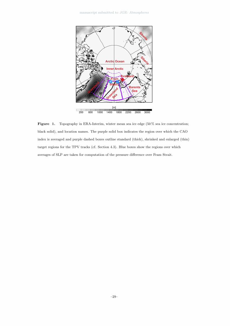
Figure captions753
Figure 1: Topography in ERA-Interim, winter mean sea ice edge (50 % sea ice con-754
centration; black solid), and location names. The purple solid box indicates the region755
over which the CAO index is averaged and purple dashed boxes outline standard (thick),756
shrinked and enlarged (thin) target regions for the TPV tracks (cf. Section 4.3). Blue757
boxes show the regions over which averages of SLP are taken for computation of the pres-758
sure difference over Fram Strait.759
Figure 2: Interannual variability of the wintertime 6-hourly CAO index (θSST−760
θ900) averaged over the Fram Strait box (see Fig. 1) with whiskers indicating the 10th−761
90th percentile range. The top 100 CAO events with and without TPVs are marked by762
triangles and circles, respectively. TPV association is evaluated wrt. the standard box763
(Fig. 1). Further shown are the threshold for CAO identification (red dashed) and the764
linear regression of the seasonal 90th percentile of the CAO index (red solid line). Thin765
red lines indicate the confidence intervals at the 95 % level for the linear regression.766
Figure 3: Evolution of the CAO index (black; θSST−θ900) averaged over the Fram767
Strait box (see Fig. 1) and the east-west pressure gradient across Fram Strait at 80.5◦N768
(gray bars) from 0000 UTC 8 Jan to 1800 UTC 30 Jan 1981. The peaks of the CAO events769
are marked by I - III and blue bars indicate the periods during which the TPV track is770
in the vicinity of Fram Strait (purple, thick dashed box Fig. 1). The CAO index is av-771
eraged over the region 20◦W - 14◦E and 71◦N - 81◦N (purple, solid box in Fig. 1) and772
the pressure gradient is computed from the difference of SLP averaged over the blue boxes773
in Fig. 1.774
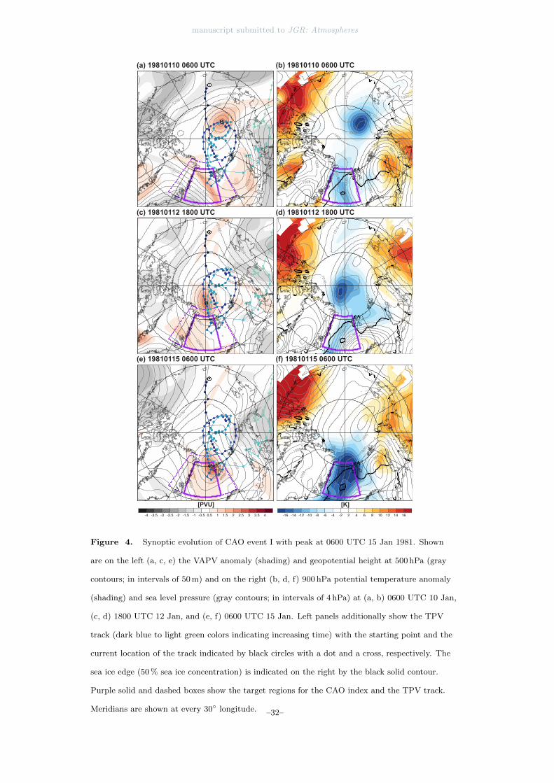
Figure 4: Synoptic evolution of CAO event I with peak at 0600 UTC 15 Jan 1981.775
Shown are on the left (a, c, e) the VAPV anomaly (shading) and geopotential height at776
500 hPa (gray contours; in intervals of 50 m) and on the right (b, d, f) 900 hPa poten-777
tial temperature anomaly (shading) and sea level pressure (gray contours; in intervals778
of 4 hPa) at (a, b) 0600 UTC 10 Jan, (c, d) 1800 UTC 12 Jan, and (e, f) 0600 UTC 15779
Jan. Left panels additionally show the TPV track (dark blue to light green colors indi-780
cating increasing time) with the starting point and the current location of the track in-781
dicated by black circles with a dot and a cross, respectively. The sea ice edge (50 % sea782
ice concentration) is indicated on the right by the black solid contour. Purple solid and783
–26–
manuscript submitted to JGR: Atmospheres
dashed boxes show the target regions for the CAO index and the TPV track. Meridi-784
ans are shown at every 30◦ longitude.785
Figure 5: As Fig. 4 but for CAO events II and III with peaks at 0000 UTC 24 Jan786
and 1200 UTC 27 Jan 1981, respectively. Fields are shown at (a, b) 1200 UTC 22 Jan,787
(c, d) 0000 UTC 24 Jan, and (e, f) 1200 UTC 27 Jan.788
Figure 6: Vertical section across TPV (see Fig. 7a) at 0600 UTC 10 Jan 1981 show-789
ing (a) potential vorticity and (b) potential temperature anomaly. Further shown are790
potential temperature (thin black; in intervals of 3 K) and the 2-PVU contour (solid black).791
Crosses indicate the location of kinematic backward trajectories from Fram Strait released792
between 24 h to 0 h prior to the peak of CAO event I (cf. Fig. 7a) and that at 0600 UTC793
10 Jan 1981 have a distance of less than 200 km from the cross section. Note that the794
different colors of the crosses in (a) and (b) have no meaning and are chosen to maxi-795
mize visibility.796
Figure 7: Location of CAO air parcel trajectories from Fram Strait contributing797
to CAO events (a) I and (b) III. Shown are 500 hPa geopotential height (purple; in in-798
tervals of 75 hPa) and the locations of backward trajectories (indicated by X labels) re-799
leased from Fram Strait 24 h (light gray), 18 h (dark gray), 12 h (cyan), 6 h (blue), and800
0 h (dark blue) before the peak of the respective event at (a) 0600 UTC 10 Jan and (b)801
0000 UTC 25 Jan. Additionally shown are trajectory locations at the peak times of the802
events (dots) and backward trajectories initialized at the peak of the event with colors803
indicating pressure along the trajectories. The black, solid line in (a) marks the cross804
section shown in Fig. 6 and the black boxes in (a, b) show the CAO target region. Merid-805
ians are shown at every 30◦ longitude.806
Figure 8: Temporal evolution of median potential temperature (θ) vs. climato-807
logical potential temperature (θc) for CAO trajectories initialized during the day before808
the peaks of CAO events I and III at 0600 UTC 15 Jan 1981 (orange) and 1200 UTC809
27 Jan 1981 (purple), respectively. White filled black triangles and circles indicate t =810
−240 h and t = 0 h. Dashed gray lines show negative potential temperature anomaly.811
Figure 9: Boxplots of (a) potential temperature 10-days prior to arriving in Fram812
Strait (at t = −240 h), (b) mean diabatic cooling rate, and (c) mean diabatic heating813
rate along 10-day backward trajectories from Fram Strait (see text for details). Black814
–27–

manuscript submitted to JGR: Atmospheres
lines, boxes, and whiskers denote the median, the interquartile range, and the 10th to815
90th percentile range, respectively. (d) Residence time of trajectories in the Arctic (pole-816
ward of 70◦N over sea ice or land). Trajectories are grouped into NO-CAO (red), ALL-817
CAO (light blue), E100-CAO (blue), and E20-CAO (dark blue) trajectories.818
Figure 10: Probability for trajectories to be at a certain location (black contours)819
and difference for ALL-CAO trajectories only wrt. all Fram Strait trajectories (shad-820
ing) at (a) t = −240 h and (b) t = −48 h in units of h(105 km2)−1. The purple box821
indicates the CAO target region. Meridians are shown at every 30◦ longitude.822
Figure 11: Temporal evolution of medians of (a) θ vs. θc and (b) latitude vs. θc823
for Fram Strait trajectories. White filled black triangles and circles indicate t = −240 h824
and t = 0 h, respectively, and colored dots show the medians in 6-hourly intervals. Group-825
ing of trajectories is as in Fig. 9. Dashed gray lines in (a) show negative potential tem-826
perature anomalies and labels (1) - (4) indicate the four main phases of trajectory evo-827
lution for the E20-CAO category (see text for details).828
Figure 12: Percentage of CAO events sorted by intensity that are associated with829
a TPV within 24 h prior to peak of CAO events. The associations are shown for the stan-830
dard box and for boxes shrinked and enlarged by 200 km in the north-south and west-831
east directions (left- and rightmost bars). See Fig. 1 for an outline of the boxes and text832
for details about the matching procedure. Gray bars denote the frequency of randomly833
chosen 24 h intervals that feature a TPV during at least one 6-hourly timestep in the re-834
spective box.835
–28–
manuscript submitted to JGR: Atmospheres
Arctic Ocean
Inner Arctic
Fram
Greenlan
d
SeaGree
nland
Siberia
BarentsSea
Strait
Siberia
Svalbard
Figure 1. Topography in ERA-Interim, winter mean sea ice edge (50 % sea ice concentration;
black solid), and location names. The purple solid box indicates the region over which the CAO
index is averaged and purple dashed boxes outline standard (thick), shrinked and enlarged (thin)
target regions for the TPV tracks (cf. Section 4.3). Blue boxes show the regions over which
averages of SLP are taken for computation of the pressure difference over Fram Strait.
–29–

manuscript submitted to JGR: Atmospheres
●●● ●● ●●● ● ●● ●●●
●●●● ●● ● ●● ●●● ● ●● ●● ●●● ● ●●● ● ●● ● ●● ●● ●● ●● ●● ●● ●● ● ● ●● ●● ●● ● ●●● ● ●●
−50
510
1520
1980 1985 1990 1995 2000 2005 2010 2015
DTH
[K]
top 1−20top 21−40
top 41−60top 61−80
top 81−100●
with TPVwithout TPV
CA
O in
dex
[K]
Figure 2. Interannual variability of the wintertime 6-hourly CAO index (θSST − θ900) aver-
aged over the Fram Strait box (see Fig. 1) with whiskers indicating the 10th − 90th percentile
range. The top 100 CAO events with and without TPVs are marked by triangles and circles,
respectively. TPV association is evaluated wrt. the standard box (Fig. 1). Further shown are
the threshold for CAO identification (red dashed) and the linear regression of the seasonal 90th
percentile of the CAO index (red solid line). Thin red lines indicate the confidence intervals at
the 95 % level for the linear regression.
–30–
manuscript submitted to JGR: Atmospheres
−2
0
2
4
6
[ hPa
/ (1
00 k
m) ]
x
data
.dth
[ind.
dth]
8 10 12 14 16 18 20 22 24 26 28 30
0
4
8
12
16
20
Day in January 1981
[ K ]
I II III
TPV TPVpres
sure
diff
eren
ce [
hPa
(100
km
)-1 ]
CA
O in
dex
[ K ]
day in January 1981
Figure 3. Evolution of the CAO index (black; θSST − θ900) averaged over the Fram Strait
box (see Fig. 1) and the east-west pressure gradient across Fram Strait at 80.5◦N (gray bars)
from 0000 UTC 8 Jan to 1800 UTC 30 Jan 1981. The peaks of the CAO events are marked by
I - III and blue bars indicate the periods during which the TPV track is in the vicinity of Fram
Strait (purple, thick dashed box Fig. 1). The CAO index is averaged over the region 20◦W -
14◦E and 71◦N - 81◦N (purple, solid box in Fig. 1) and the pressure gradient is computed from
the difference of SLP averaged over the blue boxes in Fig. 1.
–31–
manuscript submitted to JGR: Atmospheres
(b) 19810110 0600 UTC(a) 19810110 0600 UTC
(d) 19810112 1800 UTC(c) 19810112 1800 UTC
(f) 19810115 0600 UTC(e) 19810115 0600 UTC
(d) 19810112 1800 UTC
[PVU] [K]
Figure 4. Synoptic evolution of CAO event I with peak at 0600 UTC 15 Jan 1981. Shown
are on the left (a, c, e) the VAPV anomaly (shading) and geopotential height at 500 hPa (gray
contours; in intervals of 50 m) and on the right (b, d, f) 900 hPa potential temperature anomaly
(shading) and sea level pressure (gray contours; in intervals of 4 hPa) at (a, b) 0600 UTC 10 Jan,
(c, d) 1800 UTC 12 Jan, and (e, f) 0600 UTC 15 Jan. Left panels additionally show the TPV
track (dark blue to light green colors indicating increasing time) with the starting point and the
current location of the track indicated by black circles with a dot and a cross, respectively. The
sea ice edge (50 % sea ice concentration) is indicated on the right by the black solid contour.
Purple solid and dashed boxes show the target regions for the CAO index and the TPV track.
Meridians are shown at every 30◦ longitude. –32–

manuscript submitted to JGR: Atmospheres
(b) 19810122 1200 UTC(a) 19810122 1200 UTC
(d) 19810112 1800 UTC(c) 19810124 0000 UTC
(f) 19810127 1200 UTC(e) 19810127 1200 UTC
(d) 19810124 0000 UTC
[PVU] [K]
Figure 5. As Fig. 4 but for CAO events II and III with peaks at 0000 UTC 24 Jan and 1200
UTC 27 Jan 1981, respectively. Fields are shown at (a, b) 1200 UTC 22 Jan, (c, d) 0000 UTC 24
Jan, and (e, f) 1200 UTC 27 Jan.
–33–

manuscript submitted to JGR: Atmospheres
(a) (b)
[hP
a]
[hP
a]
[PVU] [K]
Figure 6. Vertical section across TPV (see Fig. 7a) at 0600 UTC 10 Jan 1981 showing (a)
potential vorticity and (b) potential temperature anomaly. Further shown are potential temper-
ature (thin black; in intervals of 3 K) and the 2-PVU contour (solid black). Crosses indicate the
location of kinematic backward trajectories from Fram Strait released between 24 h to 0 h prior to
the peak of CAO event I (cf. Fig. 7a) and that at 0600 UTC 10 Jan 1981 have a distance of less
than 200 km from the cross section. Note that the different colors of the crosses in (a) and (b)
have no meaning and are chosen to maximize visibility.
–34–
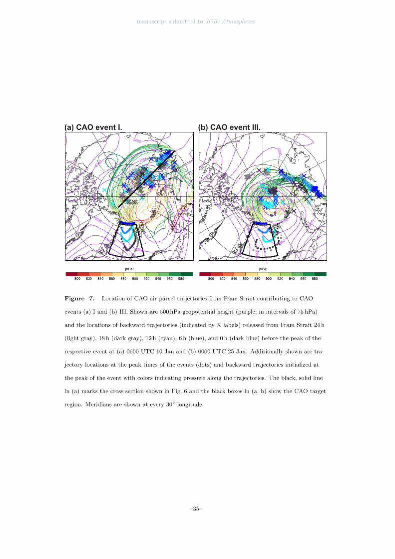
manuscript submitted to JGR: Atmospheres
(a) CAO event I. (b) CAO event III.
Figure 7. Location of CAO air parcel trajectories from Fram Strait contributing to CAO
events (a) I and (b) III. Shown are 500 hPa geopotential height (purple; in intervals of 75 hPa)
and the locations of backward trajectories (indicated by X labels) released from Fram Strait 24 h
(light gray), 18 h (dark gray), 12 h (cyan), 6 h (blue), and 0 h (dark blue) before the peak of the
respective event at (a) 0600 UTC 10 Jan and (b) 0000 UTC 25 Jan. Additionally shown are tra-
jectory locations at the peak times of the events (dots) and backward trajectories initialized at
the peak of the event with colors indicating pressure along the trajectories. The black, solid line
in (a) marks the cross section shown in Fig. 6 and the black boxes in (a, b) show the CAO target
region. Meridians are shown at every 30◦ longitude.
–35–
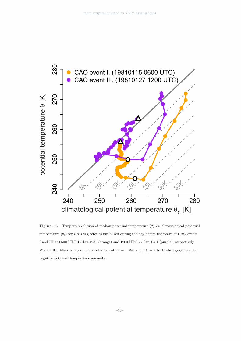
manuscript submitted to JGR: Atmospheres
times
data
.th.p
erc[
, 3]
−240 −192 −144 −96 −48 0 48
240
250
260
270
280
[h]
pote
ntia
l tem
pera
ture
[K]
data.thcl.perc[, 3]
data
.th.p
erc[
, 3]
●●●●●●●●●●●●●●●●●●●●●●●●●●●●●●●●●●●●●●●● ● ●
●
●
●
●
●
●●
●●●●●●
●●●●●●●●●●●●●●●●●
●●●●●●●●●
●●●●●●● ●
● ●
●
●
●
●●●●
●
●
240 250 260 270 280
240
250
260
270
280
pote
ntia
l tem
pera
ture
[K]
climatological potential temperature [K]
●
●
CAO event I. (19810115 0600 UTC)CAO event III. (19810127 1200 UTC)
climatological potential temperature qC [K]
5K 10K
15K
25K
30K
35K
20K
pote
ntia
l tem
pera
ture
q [K
]
Figure 8. Temporal evolution of median potential temperature (θ) vs. climatological potential
temperature (θc) for CAO trajectories initialized during the day before the peaks of CAO events
I and III at 0600 UTC 15 Jan 1981 (orange) and 1200 UTC 27 Jan 1981 (purple), respectively.
White filled black triangles and circles indicate t = −240 h and t = 0 h. Dashed gray lines show
negative potential temperature anomaly.
–36–

manuscript submitted to JGR: Atmospheres
0.0
0.5
1.0
1.5
2.0
2.5
3.0
3.5
4.0
diab
atic
hea
ting
[K /
day]
240
250
260
270
280
290
pote
ntia
l tem
pera
ture
at t
=−24
0h [K
](a) (b) (c)
−4.0
−3.0
−2.0
−1.0
0.0
diab
atic
coo
ling
[K /
day]
0−1 1−2 2−3 3−4 4−5 5−6 6−7 7−8 8−9 > 9
# days in Arctic
[%]
010
2030
40
no CAO traj.all CAO traj. (DTH > 90th perc)all CAO eventstop 20 CAO events
NO-CAOALL-CAOE100-CAOE20-CAO
(d)
Figure 9. Boxplots of (a) potential temperature 10-days prior to arriving in Fram Strait (at
t = −240 h), (b) mean diabatic cooling rate, and (c) mean diabatic heating rate along 10-day
backward trajectories from Fram Strait (see text for details). Black lines, boxes, and whiskers de-
note the median, the interquartile range, and the 10th to 90th percentile range, respectively. (d)
Residence time of trajectories in the Arctic (poleward of 70◦N over sea ice or land). Trajectories
are grouped into NO-CAO (red), ALL-CAO (light blue), E100-CAO (blue), and E20-CAO (dark
blue) trajectories.
–37–

manuscript submitted to JGR: Atmospheres
(a) t = -240h
[ ‰ (105 km2)-1][ ‰ (105 km2)-1]
(b) t = -48h
Figure 10. Probability for trajectories to be at a certain location (black contours) and differ-
ence for ALL-CAO trajectories only wrt. all Fram Strait trajectories (shading) at (a) t = −240 h
and (b) t = −48 h in units of h(105 km2)−1. The purple box indicates the CAO target region.
Meridians are shown at every 30◦ longitude.
–38–

manuscript submitted to JGR: Atmospheres
data.thcl.nocao_traj.perc[, 3]
data
.th.n
ocao
_tra
j.per
c[, 3
] ●●●●●●●●●●●●●●●●●●●●●●●●●●●●●●●●●●●●●●●● ● ●
●
●
●
●
●
●
●
●●●●
●●●●●
●●●●●●●●●●
●●●●●●●●●●●●●●●●●●●● ● ● ●
●
●
●
●
●
●
●
●●●●●
●●●
●●●●●●●●●●●●●●
●●●●●●●●●●●●●●●●
●● ●
●
●
●
●
●
●
●●
●●●●●●●●●●●●●●●●●●●●●●●●●●●●●●●●●●●●●●●●●●●●●●●●
●
●
●
●
●
245
250
255
260
265
270
275
280
245 250 255 260 265 270 275 280
pote
ntia
l tem
pera
ture
[K]
climatological potential temperature [K]
●
●
●
●
no CAO traj.all CAO traj. (DTH > 90th perc)all CAO eventstop 20 CAO events
5K 10K
15K
25K
30K
20K
data.thcl.nocao_traj.perc[, 3]
data
.lat.n
ocao
_tra
j.per
c[, 3
]
●●●●
●●●●
●●●●
●●●●●
●●●●●
●●●●●●●●●●●●●●●●●
●●
●
●●●●●●
●
●
●●●●●
●●●●
●●●●
●●●●
●●●●●●●●●●●●●●●●
●
●●●●●
●
●
●
●
●
●
●
●
●
●
●
●●●●●
●●●●
●●●●
●●●●
●●●●●
●●●●
●●●●●
●
●
●
●
●
●●●
●
●
●
●
●
●
●
●
●
●
●
●●●●●●
●●●●●●●●●●●●●●●
●●●●●●●●●●●●●●
●
●● ●
●
●
●
●
●
●
●
●
●
●
●
6065
7075
8085
90
245 250 255 260 265 270 275 280
latit
ude
[°]
climatological potential temperature [K]
●
●
●
●
no CAO traj.all CAO traj. (DTH > 90th perc)all CAO eventstop 20 CAO events
(a) (b)
NO-CAOALL-CAOE100-CAOE20-CAO
(1)
(2)
(3)
(4)
climatological potential temperature qC [K]
pote
ntia
l tem
pera
ture
q [K
]
climatological potential temperature qC [K]
latit
ude
[°]
(1)
(2)
(3)
(4)
Figure 11. Temporal evolution of medians of (a) θ vs. θc and (b) latitude vs. θc for Fram
Strait trajectories. White filled black triangles and circles indicate t = −240 h and t = 0 h, re-
spectively, and colored dots show the medians in 6-hourly intervals. Grouping of trajectories is
as in Fig. 9. Dashed gray lines in (a) show negative potential temperature anomalies and labels
(1) - (4) indicate the four main phases of trajectory evolution for the E20-CAO category (see text
for details).
–39–
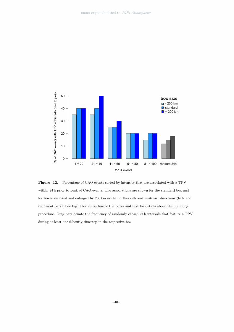
manuscript submitted to JGR: Atmospheres
1 − 20 21 − 40 41 − 60 61 − 80 81 − 100 random 24h
[%]
0
10
20
30
40
50
% o
f CAO
eve
nts
with
TP
V w
ithin
24h
prio
r to
peak
top X events
box size− 200kmnormal+ 200km
box size
standard+ 200 km
- 200 km
Figure 12. Percentage of CAO events sorted by intensity that are associated with a TPV
within 24 h prior to peak of CAO events. The associations are shown for the standard box and
for boxes shrinked and enlarged by 200 km in the north-south and west-east directions (left- and
rightmost bars). See Fig. 1 for an outline of the boxes and text for details about the matching
procedure. Gray bars denote the frequency of randomly chosen 24 h intervals that feature a TPV
during at least one 6-hourly timestep in the respective box.
–40–