r

N A S A T E C H N I C A L N A S A T R R-2 5 1 4# R E P O R T

G; P

m

~ 3 ON THE THEORY AND METHODS OF STATISTICAL INFERENCE (2

b j Z e r d l d L. Smith F )J;$++ i!t nzes Research Center

Moffett Field, Cal$ 3

k i f ' ' ] b

N A T I O N A L A E R O N A U T I C S A N D SPACE A D M I N I S T R A T I O N G A P Y L 1 9 6 7

https://ntrs.nasa.gov/search.jsp?R=19670012710 2018-08-26T09:05:45+00:00Z

ON T H E THEORY AND METHODS

O F STATISTICAL INFERENCE

By G e r a l d L. Smith

A m e s R e s e a r c h C e n t e r Moffet t Field, Calif.

NATIONAL AERONAUTICS AND SPACE ADMINISTRATION

NASA TR R-251

For sale by the Clearinghouse for Federal Scientific and Technical Information Springfield, Virginia 22151 - CFSTI price $3.00

ON THE THEORY AND METHODS OF STATISTICAL INFERENCE

By Gerald L. Smith Ames Research Center

SUMMARY

Statistical inference is the process of intelligently using information from observations and experiments to draw conclusions and make decisions. The class of inference problems includes all the classical statistical problems of point and parameter estimation, re - gression analysis, and hypothesis testing, a s well as the engineering problems of control and filtering.

In order that inference problems may be stated in mathematical terms, it is neces- sa ry to utilize mathematical measures of the often intangible entities called knowledge and goodness (or optimality). Probability is the measure utilized for knowledge, and loss functions serve as measures of optimality. The conversion of knowledge and good- ness into functional or numerical t e rms is usually quite subjective and thus to a sub- stantial extent arbitrary. Nevertheless, the conversion is necessary if the language of mathematics is to be employed in the inference logic.

The various mathematical methods developed, under different assumptions, for solving inferential problems are unavoidably related since all a re (in principle) reducible to a common form. Some of the most fundamental of these--least squares, minimum variance, and maximum likelihood--are reviewed to show their interrelationships. The newer developments of sequential analysis and filtering a re similarly described. All of these a re shown to be special casesof the general theory of Bayesian decision making.

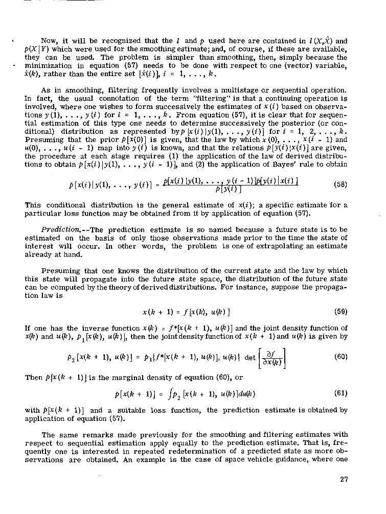
The Bayesian decision theory requires the specification of an appropriate loss function. The optimum decision is then defined as that which minimizes the mathematical expectation of this loss. Computation of this expectation requires obtaining the posterior distribution of the unknown state based on prescribed scientific observations.

Under restrictive conditions the computations involved in this general decision- making procedure a re reducible to relatively simple forms. For application under more general conditions methods of approximation and efficient computational algorithms a re presently being developed.

INTRODUCTION

The methods of statistics and modern filter theory a re finding ever increasing application in present-day scientific and engineering problems because of the power and universality of these methods. However, an individual attempting to use statistical

techniques often has not had the opportunity to acquire a knowledge of the underlying principles and thus may find himself bewildered by the vast array of literature from which he seeks to extract techniques suitable for his problem.

One of the situations in which this difficulty has appeared is in the application of the Kalman filter theory to space vehicle navigation (refs. 1 and 2). This is a problem in trajectory determination for the solution of which the methods of least squares and maximum likelihood have also been applied, and it is natural to ask what a r e the dif- ferences between the methods--that is, whether the new method is better than the old. Answers to such questions can be made only by examining the foundations of the methods, which can be shown to belong to the same basic theory. A s one investigator (ref. 3) says, "Diversified fields of scientific inquiry demand somewhat different and specialized tech- niques in particular problems; yet the fundamental principles which underlie all the vari- ous methods a re identical regardless of the field of application.''

It is the purpose of this paper to present a unified summary of several specialized techniques, showing how they a re related to the general theory of statistical inference. The paper begins with a brief description of (1) the general principles of statistical inference and areas of their application in science and engineering, and (2) the prob- ability and optimality concepts which a r e the foundations of the theory. Then the develop- ment of the specific techniques is outlined to show their differences and similarities.

The treatment used here does not involve esoteric mathematics and car r ies no pretense of completeness or rigor. By keeping the development simple, it is hoped that a certain class of readers can be helped to a greater insight, a better feeling for the choice of specialized methods, and a more knowledgeable interpretation of results obtained therefrom. For actual use of the particular techniques, the reader must under- take a more intensive study, using the extensive literature, only a small part of which is referenced herein.

SYMBOLS

"ij

A

B

C

d(x 1 D

element in ith row andj th f ( x , u ) column of matrix A

matrix in linear observation F equation (24)

arbitrary matrix

G arbitrary matrix

function of x in 2

normalizing constant in nor- mal probability d e n s i t y 1

J function

K e observation error vector

E ( expectation of ( )

function of x and u in sys- tem equation (56)

matrix in linear system equation (63) function of x in observation equation (9)

matrix in linear s y s t e m equation (63) function of x and e inobser- vation equations (62) and (37) identity matrix optimality criterion func- tional gain matrix in Kalman filter equation (70)

2

loss function (sometimes a used without arguments)

6 number of observations

A probability density function of x

unknown parameter vector

decision

posterior covariance matrix of x

joint probability density func- p mode of a distribution tion of x and y

conditional probability den- sity function of x given y Q X state space

0 standard deviation

prior covariance matrix of x

covariance m a t r i x of e ; E(eeT)

covariance m a t r i x of u ; 6 m u m ( ) E ( UUT)

Notation

arg min( ) set of 6 generating the mini-

( I T transpose of the matrix ( ) random disturbance or con- trol input to system ( 1-1 inverse of the matrix ( )

positive semidefinite weight- ( A )

ing matrix

state or unknown parameter or data vector

i")

estimate of ( )

er ror in estimation of ( )

Subscripts matrix (or vector) composed of a set of Xi

observation or data vector

matrix (or vector) composed of a set of yi opt optimal

i , j ,m,n general indices

k time index

BASIC CONCEPTS IN STATISTICAL INFERENCE

The Nature of Statistical Inference

Conclusions regarding the nature of our environment have been derived from myriad observations, or physical sensations, induced by our contact with the physical world; the process of logically interpreting empirical data is termed statistical inference.

Scientific knowledge is never exact--that is, we may assume there exists some true state of things, but it is never perfectly discernible. Our "laws" and compilations of "facts" a re then simply estimates of the true state made up of economical condensations of as much as possible of our observational data. The continuing purpose of scientific

3

effort is to test these laws and facts by means of further experiments and by the process of statistical inference to refine and improve our knowledge. As Jeffreys says (ref. 4), "Scientific progress never achieves finality; it is a method of successive approximation."

Applied science is concerned with the problems of utilizing scientific knowledge in the making of decisions regarding courses of action. Clearly, since decisions depend upon knowledge and knowledge depends upon empirical data, decision making can be regarded a s the direct utilization of observations for the determination of courses of action, with or without the intermediate step of estimating the state of nature. Thus, if decisions a re thought of as inferences, then statistical inference encompasses deci- sion making as well a s estimation. In fact, by regarding estimation as "deciding" what is the true state of things, one concludes that decision making and statistical inference a r e synonymous in the broad sense.

By the foregoing argument, it is seen that all scientific effort involves statistical inference. Classical statistics, including such subjects as hypothesis testing, regression analysis, estimation, and the analysis of variance, has to do with determining the true state of things. Filter theory has to do with determining the messages contained in received signals. Control theory has to do with the design of automated systems which have the job of "deciding," on the basis of measurements of the environment, what control should be applied to a given plant. Operations research deals with decisions regarding resource allocation, scheduling, inventory control, and the like. And game theory t rea ts the problem of decision making in contests with intelligent adversaries.

To apply the methods of statistical inference to any particular scientific problem, it is f i r s t necessary to express the problem in mathematical language. This is often the most difficult step because knowledge and utility concepts--and even sometimes the data itself--frequently a re not given in numerical form. In the following sections some of the difficulties of this conversion a re discussed.

*

Probability as the equivalent of empirical knowledge. --Any numerical measure of empirical knowledge must reflect the uncertainty inherent in such knowledge. Considering that empirical knowledge consists, not in facts, but rather of se t s of propositions with varying degrees of assurance a s to their correct representation of the facts, the assign- ment of specific numerical values to these degrees of assurance will constitute an appropriate measure, provided, of course, that such assignment is logically consistent.

Historically, the first such assignment of numerical value to degrees of assurance occurred in connection with empirical data generated by repe ted random experiments, which it was observed exhibit a significant regularity. For inst 4 nce, in many throws of a t rue die, face A is found to turn up almost exactly 1/6 of the time. It is appropriate then to assume that the assurance, or probability, of obtaining result A in one throw is 1/6, and the number 1/6 then represents the empirical knowledge gained from the die experi- ments. The extension of the concept of probability to represent in a general way "degrees of reasonable belief" which a r e not necessarily based on such direct frequency ratio measurements is fairly natural. It may be observed that there is a notable lack of agreement amongst mathematicians as to the legitimacy of this more general interpreta- tion of probability. However, the arguments a r e strictly philosophical, and here we choose to employ the general definition because it permits u s to characterize all empirical knowledge in the same way so that we may then apply the entire body of probability theory to the general problem of statistical inference.

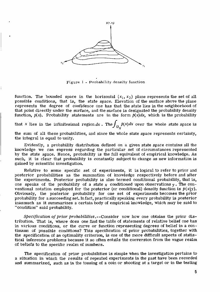
A complete set of probabilistic statements (or likelihood measures) is called a prob- ability distribution and is, of course, defined on the set of all possible states. The idea of a distribution is illustrated in figure 1, which represents a continuous probability density

4

Figwe 1 - Probability density function

function. The bounded space in the horizontal (XI, x2) plane represents the set of all possible conditions, that is, the state space. Elevation of the surface above the plane represents the degree of confidence one has that the state l ies in the neighborhood of that point directly under the surface, and the surface is designated the probability density function, p(x) . Probability statements a re in the form p(x)dx, which is the probability I that x. l ies in the infinitesimal region dx . T h e j P ( X ) h over the whole state space is

QX

the sum of all these probabilities, and since the whole state space represents certainty, the integral is equal to unity.

Evidently, a probability distribution defined on a given state space contains all the knowledge we can express regarding the particular set of circumstances represented by the state space. Hence, probability is the full equivalent of empirical knowledge. As such, it is clear that probability is constantly subject to change as new information is gained by scientific investigation.

Relative to some specific set of experiments, it is logical to refer to prior and posterior probabilities a s the summation of knowledge respectively before and after the experiments. Posterior probability is also termed conditional probability, that is, one speaks of the probability of a state x conditioned upon observations y . The con- ventional notation employed for the posterior (or conditional) density function is p(x)y). Obviously, the posterior probability for one set of experiments becomes the prior probability for a succeeding set. In fact, practically speaking every probability is posterior inasmuch as it summarizes a certain body of empirical knowledge, which may be said to "condition" said probability.

Specification of pr ior probabilities.--Consider now how one obtains the prior dis- tribution. That is, where does one find the table of statements of relative belief one has in various conditions, or the curve or function representing degrees of belief in a con- tinuum of possible conditions? This specification of prior probabilities, together with the specification of an optimality criterion, is one of the more difficult aspects of statis- tical inference problems because it so often entails the conversion from the vague realm of beliefs to the specific realm of numbers.

The specification of prior probabilities is simple when the investigation pertains to a situation in which the results of repeated experiments in the past have been recorded and summarized, such as in the tossing of a coin o r shooting at a target or in the testing

5

of items from a production line. In such cases it is known that the results were sometimes state A , sometimes state B , etc., and the prior distribution is given directly by the relative frequencies of the various occurrences.

What does one do, however, in a less objective investigation, such as determining whether or not there is life on Mars? Our prior belief (or disbelief) in life on Mars is real enough, being based on quantities of information obtained in assorted observations. This information has to be sensibly organized and analyzed to make the required prob- abilistic statements. If the data are insufficient to perform the analysis, we could simply make a knowledgeable judgment. Raiffa and Schlaifer (ref. 5) state that, "In such situa- tions the prior distribution represents simply and directly the betting odds with which the responsible person wishes his final decision to be consistent.''

This goes against the grain for many meticulous scientists, who often say that no probability statements can be made in such circumstances. But surely this is unduly pessimistic. The summation of our information at any particular point in scientific investigations can not be ignored, and probability statements a re the only appropriate way of reflecting this knowledge.

As pointed out by Raiffa and Schlaifer, the psychological difficulty of assigning "betting odds" to express the investigator's belief in the state of affairs is so great that he will generally be reluctant to specify the distribution in any more detail than by a few summary measures, such as the mean and a percentile or two. From this point on, he is likely to settle for a representation of the distribution by any reasonable form which fits these minimum specifications. This practice accounts, in part at least, for the wide- spread use of simple distributions such a s the normal, which is so easily specified by two parameters (i.e., the mean and variance).

The wide variety of special methods for the solution of statistical inference prob- lems which f i l l the literature reflects a variety of different assumptions regarding prior probability. These range from complete ignorance of the distribution, as is typical in regression analysis and least-squares techniques, to complete knowledge, that is, the prior distribution completely specified. Neither of these assumptions is ever wholly correct. Total ignorance is implausible in the statement of any problem, and perfect knowledge is equally implausible from the argument of subjectivity which implies that nothing is ever known perfectly. However, the assumptions can usually be rationalized i n terms of approximations to the true situation. When prior knowledge is assumed totally lacking what one really means is that the bulk of the information regarding the state is contained in the observations, so that for practical purposes prior knowledge may as well be ignored. When some type of "perfect" prior knowledge is assumed, one really means that the prior knowledge is already so good with respect to the information contained in the observations that the latter cannot be expected materially to improve the estimate.

One often has to be cautious, of course, in assuming any kind of "perfect" prior knowledge. Even though prior knowledge may be extremely good with respect to a certain body of data, there may always come a time with continued experimentation that the as- sumption is no longer valid. For example, in the determination of the trajectory of a space vehicle from tracking data, the astrodynamic constants (e.g., mass of the earth, astronomical unit, etc.) may be considered to be known perfectly at first, relative to a small amount of data. But after much trackingdata has been accumulated, it will be found that e r ro r s in the constants can be detected, that is, the estimates of the constants can be improved,

6

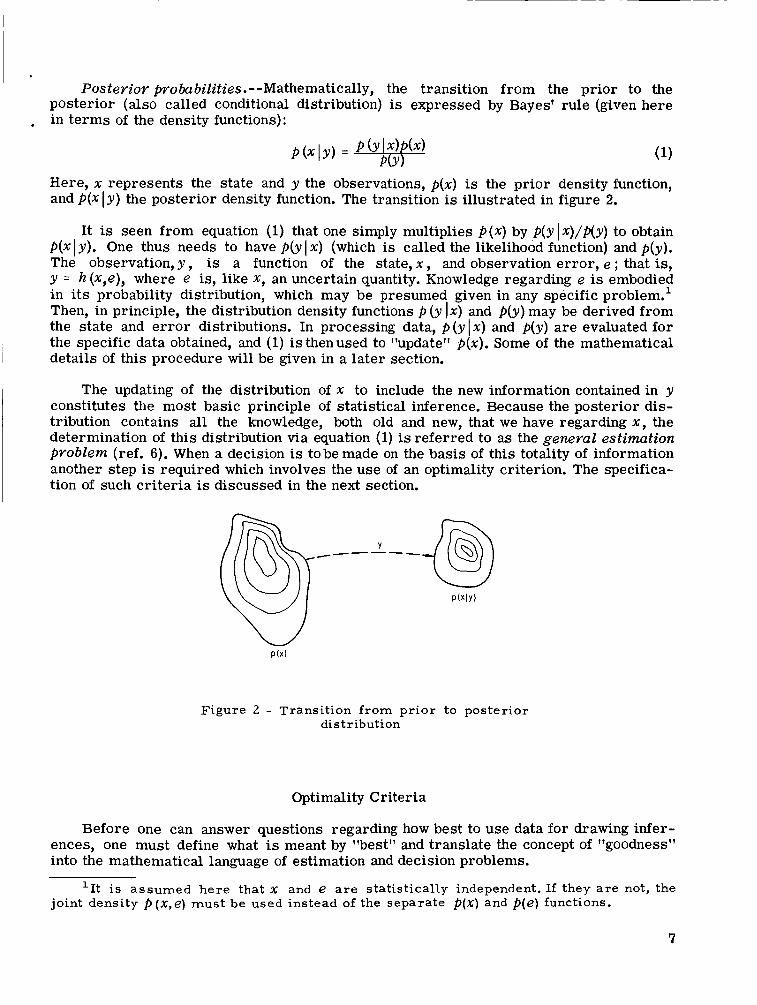
I . Posterior probabilities.--Mathematically, the transition from the prior to the

posterior (also called conditional distribution) is expressed by Bayes' rule (given here in te rms of the density functions): .

Here, x represents the state and y the observations, p(x) is the prior density function,

It is seen from equation (1) that one simply multiplies P(x) by P(YIx)/P(Y) to obtain p(xly). One thus needs to have p(yl x) (which is called the likelihood function) and p(y). The observation, y , is a function of the state, x , and observation error , e ; that is, y = h @,e), where e is, like X, an uncertain quantity. Knowledge regarding e is embodied in its probability distribution, which may be presumed given in any specific problem.' Then, in principle, the distribution density functions p (y l x ) and p(y) may be derived from the state and e r r o r distributions. In processing data, p (y I x) and p(y) a r e evaluated for the specific data obtained, and (1) is then used to "update" p(x). Some of the mathematical details of this procedure will be given in a later section.

l and P(x I y) the posterior density function. The transition is illustrated in figure 2.

The updating of the distribution of x to include the new information contained in y constitutes the most basic principle of statistical inference. Because the posterior dis- tribution contains all the knowledge, both old and new, that we have regarding x, the determination of this distribution via equation (1) is referred to as the general estimation problem (ref. 6). When a decision is tobe made on the basis of this totality of information another step is required which involves the use of an optimality criterion. The specifica- tion of such cr i ter ia is discussed in the next section.

c c

Figure 2 - Transition from prior to posterior distribution

Optimality Criteria

Before one can answer questions regarding how best to use data for drawing infer- ences, one must define what is meant by T7best" and translate the concept of "goodness" into the mathematical language of estimation and decision problems.

'It is assumed he re that x and e a r e statistically independent. If they a r e not, the joint density P(x,e) must be used instead of the separate p ( X ) and p(e) functions.

7

The principle of least squares was perhaps the earliest development in the concept of optimality. It was originally developed as a means of solving two types of problems. Problems of the first type ar ise when repeated measurements of some phenomenon do not always give the same result, and one wishes to remove the apparent inconsistencies in the data, such as in the determination of the orbits of planets f rom a large number of line-of -sight observations. Problems of the second type a re simply curve-fitting situations (or regression analysis), where it is desired to summarize data in the more manageable form of simple functional relationships (often linear) or at least in the form of a smooth curve. In these applications "best" means that the solution minimizes the sum of squares of deviations between data points and corresponding points derived from the solution.

-

The difficulty with least squares is that i t suse is not based on a clear-cut optimality principle but rather on the fact that its use leads to simple linear operations upon the data. There is no reason per s e why a "better" solution might not be obtained by mini- mizing, for instance, the sum of absolute values of the deviations. Of course, it can be argued that the latter approach requires fa r more difficult computations, so that "best" in the broad sense should take this into account and assign a plus value to the least squares procedure.

A more precise definition of optimality is obtained by invoking the concept of the cost, 1 , associated with operations upon data. The principle involved is to design one's modus operandifor handling data (either for forming an estimate or for making an action decision) so a s to minimize the average (or expected) cost, E ( Z ) , of a single operation. A modus operandi so selected is optimal in the sense that the total cost of a large number of operations of this type would in all probability be less than for any other modus operandiof the same class.

Optimality is now dependent upon the definition of 1 for the particular application one has in mind. For instance, consider the problem of designing an operational system for tracking a space vehicle, determining its trajectory, and providing control over in-flight maneuver, possible abort, reentry, and recovery aspects of the mission. Such factors as the accuracy of the estimate, the speed with which it may be obtained, reliability and cost of complex tracking and computing equipment, the flexibility of recovery forces, etc., a r e all significant and may be combined in a variety of ways to define an optimal system. The weighting applied to each factor must be decided by engineers with, at best, an im- perfect knowledge of the true importance of each factor. Obviously, one is faced here with the same difficulty encountered in specifying prior probabilities- -namely, the con- version of subjective quantities into numerical o r functional form. Thus, the practical engineer, knowing that he can only approximate, is justified in arbitrarily choosing cost representations which a re mathematically tractable. Of course, any system so designed is optimal only with regard to the more o r less arbitrary criterion so established.

This situation has led to a dominant use of quadratic type cri teria, whose tractability is indisputable. Such criteria call for the data operations to minimize functionals of the form

J = E ( S T W f )

where W is a positive semidefinite weighting matrix, and 4 is usually a zero mean random variable defined appropriately for the problem. For instance, in the comparatively simple problem of pure estimation (Le., where the only significant cost is due to inaccuracy in the estimate), 4 would be the estimation e r ro r , 4 = P = x - 2, so that J is a measure of

8

the concentration of estimates 2 about the true value x. Indeed, J is a linear function of the second-order moments (covariances) of the 2 distribution, hence the name "mini- . mum variance" applied to one of the estimation techniques which uses this type of optimality criterion.

Whatever objections may be raised to this pre-eminent use of quadratic cri teria (which reduce to the familiar mean-square e r ror criterion for scalar x), we a re faced with the fact that most of the useful analytical methods a r e based on such criteria. Specialized analytical results occasionally have been obtained for other cri teria (refs. 7 and 8), and there has been at least one successful attempt to generalize the minimum variance solution to a broader class of cri teria (refs. 6 and 9) which will be discussed later. Beyond this, to utilize an arbitrary criterion one would be forced to use numerical methods and a large scale computer.

THE MATHEMATICS OF STATISTICAL INFERENCE

In the previous sections we have identified the basic principles of the universal notion of statistical inference. We now proceed to a review of some of the explicit mathematical methods of statistical inference. Emphasis is on showing the relation of each method to the other methods and to the general theory. It is assumed in all of the following that probability distributions, cost functions, and functional relationships be- tween variables a re given when needed--that is, the problem of translating scientific questions into suitable mathematical language has been surmounted.

Least Squares

The two types of problems ordinarily treated by least squares were described in the previous section. These problems are actually not distinct if one adopts the proper point of view, a conclusion supported by the results developed below.

Reconciliation of inconsistent data.--In this case it is assumed that the body of data to be analyzed consists of "noisy" measurements of some physical, economic, biologic, etc., phenomenon. The problem is to find anestimate of the underlying phenomenon which is consistent with the data and matches it best in a least-squares sense, under the as- sumption that the functional relation is known between the unknown quantities and the observables being measured. That is, the mathematical model of the system is given as

y i = g(x) t e i ,

where the y i e r r o r in the i th measurement, and g is a known function.

i = 1, 2,. . . N

a r e the measurements, x is the unknown quantity, e i is the "noise" o r

It is desired to determine that value of X for which the quantity

N

is a minimum. If y i is a vector (Le., several different quantities measured), then equation (3) should be written as

N

Of course, the unknown x may also be a vector.

To determine the minimum, equation (4) is differentiated with respect to x , obtaining

N rp

1

For J to be minimum, equation (5) is set equal to zero; then

1

It is not possible to write an explicit solution for the minimizing x from this equa- tion unless an analytic expression for g is given; even then the set of equations is generally nonlinear, hence often difficult to solve. However, in the common situation in which g is linear (e.g., g(x ) = Ax) the solution is straightforward. Since in this case &/ax = A, equation (6) reduces to

N

1

and the least-squares estimate of x is

N

1

N 1

N where it is seen that - 2 y i is simply the numerical average of the measurements.

1

The above solution is by no means the most general which can be handled by least squares. For instance, very commonly one has situations in which the functional relation g between the state and observables may be different (although still assumed known) for each measurement. The direct way to treat such a case is to consider the entire body of data as a single vector observation, say y . Then the system equation is

10

In the linear case y = AX t e . The equation to be solved is

(ATA)x = A y T

and the least-squares solution is simply

$ = (ATA)-' ATy

The equations represented in matrix form in equations (7) and (10) a re the so-called normal equations. It should be noted that they do not necessarily have a unique solution, depending upon whether or not the normal matrix ATA is singular. Even so, a least- squares "best" estimate can always be obtained by means of the generalized inverse (see ref. 10).

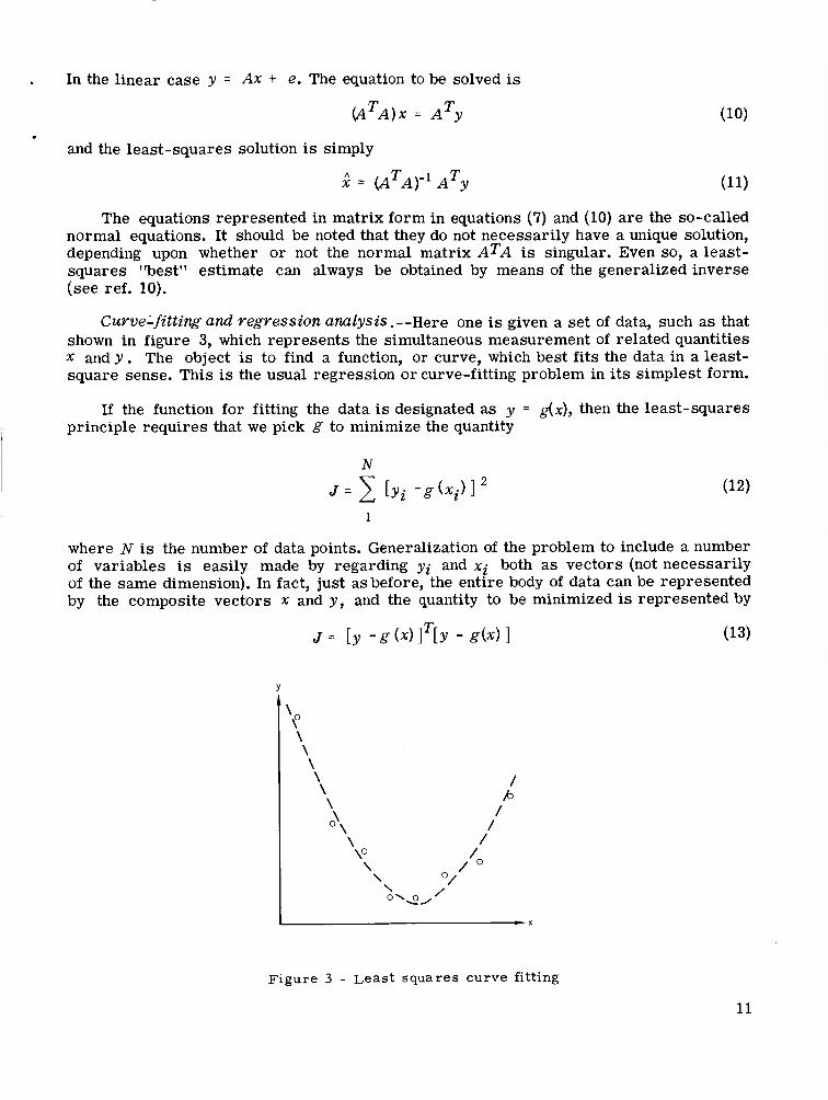
Curve-fitting and regression analysis. --Here one is given a set of data, such as that shown in figure 3, which represents the simultaneous measurement of related quantities X and Y . The object is to find a function, or curve, which best fits the data in a least- square sense. This is the usual regression or curve-fitting problem in its simplest form.

If the function for fitting the data is designated a s y = g ( ~ ) , then the least-squares principle requires that we pick g to minimize the quantity

N

1

where N is the number of data points. Generalization of the problem to include a number of variables is easily made by regarding y i and xi both as vectors (not necessarily of the same dimension). In fact, just a s before, the entire body of data can be represented by the composite vectors x and y , and the quantity to be minimized is represented by

Y

I ,X

Figure 3 - Least squares curve fitting

11

Now, it is easy to see, using figure 3 as an example, that the curve-fitting problem makes sense only if smoothing is employed. That is, obviously the curve consisting of straight line segments connecting the data points make J zero, and no better f i t can be found. But this does not effect any condensation of the data whatsoever and is thus point- less. What we need is to restrict our choice of function to a class that can be described by a number of parameters smaller than N--preferably enough smaller to obtain a significant condensation. This difference between the "dimensions" of the data and of the fitting function is often referred to as the "degrees of freedom.'' As the number of de- grees of freedom is increased the minimum obtainable J generally increases.

-

-

Presuming that a functional form for g has been selected (or perhaps is given as par t of the problem statement), describable by a certain number of parameters which a r e to be determined, the minimization procedure can proceed. Here we will consider only the case of simple linear regression, that is, g is linear in x , or g ( x ) = Ax. (It is assumed here, without loss of generality, that the data have been translated, so that the origin is at the point [(l/N) SYi, (l/N) S y i ] so as to simplify the mathematical expressions which follow.) In this case we have

N

1

where it is assumed that yi is an m vector (i.e., has m components), and xi is an n vector; A is therefore an m x n matrix of unknown regression coefficients which a r e to be determined to minimize J . The minimization is achieved in the usual way by dif- ferentiating J with respect t o A and setting the result equal to zero, where aJ/aA is defined as the matrix

Following th is procedure, we obtain N

1 and from this we must have

N N

1 1

12

N

Note that to obtain a unique solution for A the matrix 1 xixi must be nonsingular.

This requires that N, the number of data points, must be at least as great as the dimen- sionality of the x i .

1.

~

If the vectors xi and yi are arrayed in columns to form matrices as follows,

X

X

e . .

I Y = :N1l yNm

then equation (17) can be rewritten in the matrix form

AXXT= YXT

or

and

Note the similarity of equation (20) to the normal equation (10) for the point estimation problem: The roles of the independent variables and the regression coefficients a r e simply reversed. That is, in the regression problem the X and Y are given, and we a re to estimateA , whereas in the point estimation problem A and y a re given and we a re to estimate x .

Reference 11 (pp. 179-183) develops the result (eq. (21)) utilizing the principle of maximum likelihood and the assumption that the data points (xi,yi) come from a multi- variate normal distribution, and reference 12 (pp. 577-579) shows how to obtain the same result by means of the Gauss-Markov theorem. However, as has been shown here, the least-squares method does not depend on any probabilistic statements.

As a critique of least squares it should be pointed out that the method is relatively simple in that it is independent of probabilistic statements regarding the observation e r ror , e . (It may be argued that the criterion of minimization of the sum of squares of

13

residuals implies certain statistical properties of e in that only when e has such prop- er t ies is such a criterion reasonable, but this is not equivalent to a direct a priori as- sumption regarding the distribution of e . ) However, the lack of probabilistic statements regarding e car r ies with it the disadvantage that it is impossible to make any prob- abilistic statements about the least-squares estimate. For instance, from equation (1 1) it can be seen that the e r ro r in estimate x" = x - 2 in the linear case is proportional to e :

and without any knowledge of e nothing can be said about f . One can, of course, make certain ex post facto assessments, such as that if e has zero mean @ ( e ) = 0) and the e a r e independent, then Z has zero mean and the least-squares estimate is "unbiased." If, further, e has the covariance E(eeT) = Q = a21, the covariance of 5? is

which provides a measure of the precision of the estimate. There is the additional possibility, for purposes of e r ro r analysis, of examining the residual, [ y - g ( k ) 1 , which constitutes an estimate of e , and from this inferring the distribution of e . However, even this if it is to be done rationally requires some assumptions as to the character of e which a re not given i n the pure least-squares problem.

Minimum Variance and Weighted Least Squares

The so-called minimum variance estimate is usually associated with the Gauss- Markov theorem (see, e.g., refs. 12 and 13), which may be stated as follows:

Suppose we have a set of observations y , described as in the previ- ous section by

y = A x t e (24)

The matrix A is assumed known; the set of parameters represented by the vector x is unknown and is to be estimated; and e is the set of ob- servation e r r o r s with covariance matrix E (eeT) = Q.

The "best" estimate of x in the sense of beingthat estimate having minimum variance from the class of all linear unbiased estimates, is given by the solution of the normal equation

T -1 A Q A X = A ~ Q - ~ Y

or

2 = ( A T i Q- A ) - i T A Q-'y

It can be readily shown that this same equation may be obtained by minimizing in the same manner as in the last section the functional

14

which is called the "weighted" sum of squares because each element of the sum in J is multiplied by one of the elements of Q -l. Thus, the minimum variance estimate may also be called a weighted least-squares estimate.

The precision of the minimum variance estimate can be expressed easily in terms of the covariance

which is obtained by substituting equation (24) into equation (26), forming the difference X = X - 2, forming the matrix product w, and taking the expectation of the result. u

The relation of this estimate to the least-squares estimate of the previous section is easily seen. If Q is a diagonal matrix(i.e., e r rors in all of the observation components a re uncorrelated one with another) and all e r rors have equal variance cr2 then Q=021. Substituting this into equation (26), we obtain

which is precisely the least-squares estimate.

Clearly, the linear least-squares estimate can be regarded as a special case of the minimum variance estimate. Many times in applications the least-squares estimate is used simply because it is easier to compute than the minimum variance estimate or because there is some doubt about the correct Q matrix (ref. 13, p. 21). In such a case the method of least squares will still give an unbiased estimate, although it will not be the best obtainable. The loss in accuracy resulting from using least squares instead of minimum variance is analyzed in reference 14.

Note that only linear estimates have been considered here, although the results can also be applied to nonlinear systems which can be successfully linearized (Le., ac- curately approximated by linear systems). It also may be noted that only the mean (as- sumed zero here) and variance of e are given. Other properties of the distribution a re immaterial because consideration is limited to linear systems and linear estimates and because the criterion is minimization of the variance of the estimate.

It is seen that with only the first and second moments of the distribution of e given, only the corresponding moments of the distribution of 2 can be obtained. In many prac- tical problems these a re adequate, but if more general results a re required one must utilize one of the more general methods to be described later.

Maximum Likelihood

The principle of maximum likelihood for use in parameter estimation was intro- duced by R. A. Fisher in 1912 and further expanded by him in a ser ies of papers (see, e.g., ref. 15).

The basic assumption is that the observations a re random variables drawn from an infinite population whose distribution is known except for a finite number of parameters. A simple example is drawing black and white balls from an urn; the distribution is known to be binomial, but the proportion of the black to white balls is not known and must be estimated from the samples (i.e., observations).

15

Another elementary example is measuring some physical quantity (such as the speed of light) with an apparatus known to introduce normally distributed zero mean errors . The measurements can be regarded as derived from a normally distributed population with an unknown mean which is the physical quantity under investigation. By estimating the mean of this population one obtains an estimate of the unknown quantity.

.

The principle of maximum likelihood estimation is to pick as estimates of the un- known parameters those values for which the set of observations would be "most likely" to occur, where "most likely" is defined to mean maximization of the so-called likeli- hood function.

The likelihood function is nothing more than the conditional density function of the observations given the unknown parameters and, as such, can be written as p (y la) , where y represents the observation and a the parameters to be estimated. In some Of the literature the notation is P @;a) , which means simply the density function of the ob- servations; the a is included in the argument to indicate the dependence of the distribu- tion upon the unknown parameters. The effect is the same in either case, although the conditional distribution notation tends to imply that a is a random variable in its own right, and sometimes there a r e objections to this on philosophical grounds since one generally is dealing in such problems with only one specific (unknown) value of a. However, it scarcely matters in maximum likelihood whether a is or is not a random variable since its "distribution," i f any, does not enter into the ML solution.

The ML solution consists in finding that value of a for which the probability P (Y la)& is a maximum, where P(Y la)@ is the probability that the observations y will lie in the hypercube dy. Since only the density function and not dy is a function of a, we a r e con- cerned only with the maximum value of p (y I a), which with y given is a function only of a.

Examples of using the M L technique a re given in many texts (e.g., see ref. 16 fo r some elementary cases, and ref. 17 for a nonlinear problem). Here, we will develop only one case, involving the multivariate normal distribution, which serves to illustrate the principles and which we will use later for comparison with other estimation methods.

First, assume observations a re generated by the linear process

y i = A ~ x t e i

where Ai is known, and the y i and e i are, respectively, observations and observation errors . It is further assumed that the ei a r e normally distributed with zero mean. The covariances E [ eieF] can be assumed either known partly o r unknown. In the latter case these a re to be estimated from the data along with estimating the unknownx , but in general, there cannot be a greater number of unknowns than there a re observations. Note that A i may be time-varying--that is, it may be different for each value of indexi .

To put the problem in its simplest form, the set of observations is combined into a single vector variable y :

16

o r

y = A x + e

Because of the normal distribution assumption, the likelihood function can be written (ref. 13, p. 416)

where Ax is the mean of the distribution, and Q is the covariance matrix E[eeT] . In the most general problem y represents the given data and a the set of elements of x and Q which are to be estimated.

To maximize p , one can just as well maximize log p :

It is seen immediately by comparing the above with the functional (27), which is mini- mized in weighted least squares, that the maximizing x is the solution of

T -I T -I A Q A x = A Q y (34)

which is precisely the normal equation of the minimum variance o r weighted least- squares method. If Q is known, then the solution requires only the estimate of x:

T -1 -1 T -1 k = ( A Q A ) A Q y (35)

For the more general solution when some of the elements of Q are also assumed unknown, one needs to find the x and Q which simultaneously maximize log P . Some of the problems involved in doing this and some methods of solution a re given in reference 11. The results a re only incidental to the main theme of this paper.

We have given above the formal statement andan example of the maximum likelihood method, which for the case considered is seen to give precisely the same result as minimum variance estimation in the linear normally distributed case. It remains to dis- cuss some of the optimality aspects of the method.

Apparently, the statement of the ML principle involves only the intuitive idea that a "best" estimate should l ie somewhere near the peak (or maximum point) of the condi- tional density function, P (y I a). Once this principle has been accepted, one then seeks to determine just how good is such an estimate. It has been shown (refs. 18, 6) that for a regular * estimation case of the continuous type, the mean square deviation of the esti- mate from the true value satisfies the Cram&-Rao inequality:

The condition of regularity i s satisfied in most common applications and will not be dealt with here .

17

where the ai , aj are elements of the vector of unknowns, CY. That is, the symmetric matrix on the left of equation (36) is positive semi-definite, and no estimates can have a covariance matrix smaller than the second termon the left. If for a particular estimate the sign of equality holds, then this is said to be an efficient estimate, and clearly no estimate can have a smaller covariance.

The argument in favor of maximum likelihood is an indirect one to the effect that if an efficient estimate exists --that is, an estimate which achieves the smallest possible covariance matrix--then it can always be formed by the method of maximum likelihood. The difficulty is that efficient estimates exist only under fairly restrictive circum- stances. (The necessary and sufficient conditions a r e given in ref. 18.) When there is no efficient estimate, then no method of estimation can achieve the lower bound and there is no guarantee that some estimate other than ML might not be better. In fact, generally in such cases there is a better estimate than ML. Even so, the ML method is l e s s complicated to apply in many circumstances and may be used for this reason even when it is known not to be the best.

Some remarks regarding the basic hypotheses of ML estimation a r e necessary for a proper perspective of the method. It will be noted that a fundamental premise of the ML theory is that the distribution form is known with only a finite number of i t s param- e te rs to be determined, In view of the ear l ier discussion on probability, it is seen that this implies a certain amount of "perfect" prior knowledge. In fact, an explicit mathe- matical expression for the likelihood function is required before we can proceed at all.

Another basic premise of ML estimation is that there is no prior knowledge regard- ing the values of the unknown parameters, a. The validity of this assumption, of course, depends on the particular problem and involves philosophical considerations which have already been dealt with at some length.

Despite possible shortcomings, ML is clearly a more versatile method than the least squares and minimum variance techniques described in the previous sections be- cause it permits the use of a complete description of the distribution of the observation errors .

Decision Theory and Bayes' Estimation

The development given in this section is based on a decision theoretic point of view which will be seen to be general enough to encompass nearly all scientific inference prob- lems, including the special c lass arising in control. When applied to estimation, this approach is often termed Bayes' estimation after the famous Bayes' Theorem which plays a central role in the development.

The decision problem.--Let x represent the set of parameters required for making a decision, 8. Suppose further that x may take on a range of different values with prob- abilities describable by means of the density function, p ( x ) . Observations dependent upon x and subject to e r r o r s e a r e to be made:

Y = h(x,e) (37)

It is assumed that the probabilities of the e r r o r s a re known for all possible values of x , so that we have the conditional density function (or likelihood function) p (y I x ) .

18

Now, to make intelligent decisions, it is necessary to know which decisions are bad and which a re good for us. That is, all possible decisions under all possible circum- stances must be ranked and, further, assigned specific numerical values. The result is a function, I , dependent upon the true (unknown) state x and upon the decision, 6:

.

I = I (x,S)

This is called a cost or payoff or loss function, and its meaning is that if a value X = xu obtains, and the decision 6 = 6, is made, then the cost or loss is I (xa,Sa).

An optimum decision strategy may now be defined as that strategy which on the average costs the least. That is, one wishes to minimize the average loss, E [ I (x ,S) 1, over all possible x , and the optimum decision is

SoPC = arg minE[Z(x,S)] (38) s x

Of course, the decision will be based on the observations, y - that is, S = ab). To compute the expectation in equation (38), one needs the probability distribution of

x given the observations, which may be represented (for a continuous distribution) by P(x1Y). Then equation (38) becomes

s = arg min JQ ~ ( x , ~ ) p ( x l y ) dx (39) opt 6 x

In the usual problem 1 (x,S) is given, but P(xIY) must be computed as follows. Pre- sumably the functional relationship y = h &,e) (where e is the observation e r ror ) and the joint density function P(x,e) are given. These imply the knowledge of the joint dis- tribution of x and y as given by p ( x , y ) , and also the distribution of y itself which is merely the marginal distribution of (x,y). Then p ( x l y ) may be written as

This is as far as the solution can be carried in very general terms. Any further result requires specific loss and density functions. If such are given in numerical o r tabular or curve form, the calculation would have to proceed by numerical methods.

If we are so fortunate as to have an I and a p ( x 1 y ) of certain forms, further general results can be obtained. Consider first the case where the functions h(x,e), P I ( ~ , e ) , 3 and P(x) are of mathematically tractable form. If the inverse function e = h*(x,y) can be obtained, then p 2 (x ,y ) and p ( y ) are given by (ref. 19):

Subscripts a r e used here on p to avoid ambiguity when different functional forms a r e involved.

19

These can then be used in equation (40). Thus, in certain cases an explicit mathematical expression can be obtained for P (x IY) for use in equation (39).

Another potentially useful analytical result has been shown by Sherman (ref. 9) to apply for certain classes of loss and density functions. If I can be expressed as a func- tion of a single argument v such that (1) 0 5 I (v) = I ( -v) (i.e., I symmetric in v) and (2) 0 5 v1 I . v?+I ( v l ) I 1 ( v2) (i.e., I wide-sense monotonic increasing in the distance from the origin4), and if p(x(y) for the given y is unimodal (i.e., has only one local maximum) and symmetric about the mean, p, then theoptimum 6 is obtained by choosing 6 to minimize 1 (X,S). For instance, suppose I = I x - d*@) I , where & is the inverse of a function d (i.e., d [d*(S) ] = 8). Then its minimum value occurs at 6 = d(x ) , and the optimum decision is Sopt = d(p ) . The essence of this result is that under the proper conditions, the mean of the posterior distribution furnishes all the information needed to obtain the optimum decision.

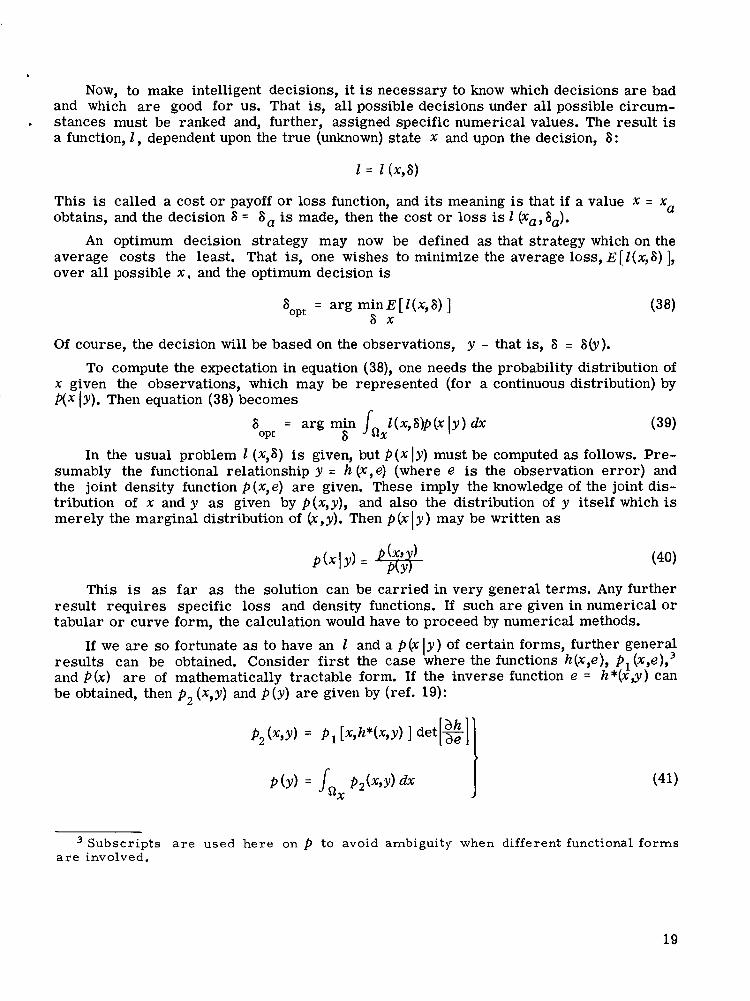
A geometrical picture is helpful to illustrate this interesting result. Figure 4 shows a loss function of the type considered. For the illustration, a problem which is single- dimensional in both x and S is employed; that is, a scalar state and scalar decision a re assumed. The loss, being a function of both x and 6 is represented by a surface whose height above the X, 8 plane is 1 , The particular form of I used here is a function symmetric in the argument [" - d*(S) 1, and monotone increasing as the magnitude of the argument increases. Thus, each cross section of I parallel to the x,Z plane is the same except for a translation in the x direction by an amount d*(S). The appearance

Figure 4 - Example loss function

Any non-negative real-valued convex function of the argument can serve a s the "distance" in this application. (See ref. 6 , p. 3 5 . )

20

’ is that of a river valley whose floor is level and t races the curve 6 = d(x) in the x,6 plane.

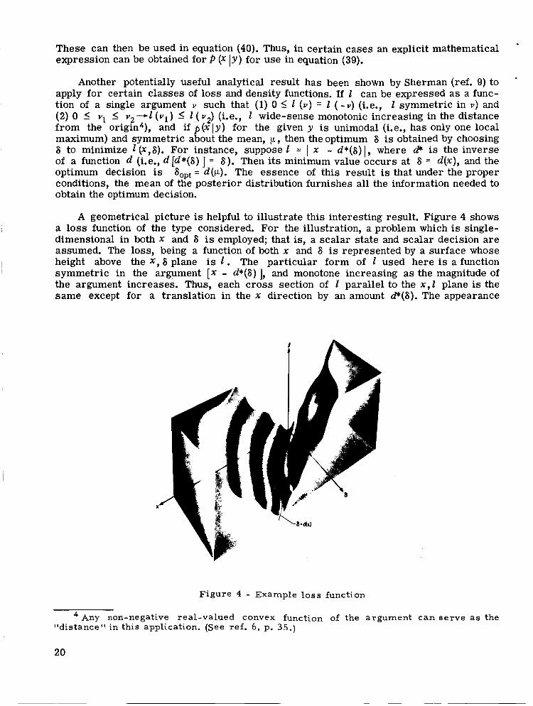
Figure 5 shows a typical symmetrical unimodal density function with a maximum at x = p, plotted on the same x , 6 base grid. Since it is not a function of 8 every cross section is the same. The comparison with a uniform mountain ridge is irresistible.

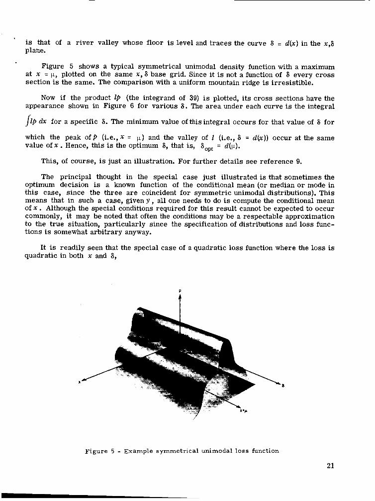
Now if the product ZP (the integrand of 39) is plotted, its cross sections have the appearance shown in Figure 6 for various 8. The a rea under each curve is the integral

JZp dx for a specific 8. The minimum value of this integral occurs for that value of 6 for

which the peak of P (i.e., x = p ) and the valley of I (i.e., 8 = d(x)) occur at the same value of x . Hence, this is the optimum 6, that is, aopt = d(p).

This, of course, is just an illustration. For further details see reference 9.

The principal thought in the special case just illustrated is that sometimes the optimum decision is a known function of the conditional mean (or median o r mode in this case, since the three a re coincident for symmetric unimodal distributions). This means that in such a case, given y , all one needs to do is compute the conditional mean of x . Although the special conditions required for this result cannot be expected to occur commonly, it may be noted that often the conditions may be a respectable approximation to the true situation, particularly since the specification of distributions and loss func- tions is somewhat arbitrary anyway.

It is readily seen that the special case of a quadratic loss function where the loss is quadratic in both x and 8,

Figure 5 - Example symmetrical unimodal loss function

21

Figure 6 - Cross sections of example lp function

I = p x - G]*C[Bx - 81

belongs to the class of loss functions described above. In this case i t can be seen that by substituting equation (42) into equation (38) and carrying out the indicated minimization the optimum decision is given by

Thus, when the loss function is quadratic the optimum decision is a linear function of the conditional expectation, regardless of the form of the conditional distribution. This, of course, reduces to the same result as the previous case when p(xly) is symmetric and unimodal, for then the mean is the same as the median and mode.

Buyes estimation. --The general decision theory solution given above is easily specialized to one of pure estimation by defining the "decision" a s one of simply deter- mining, as accurately as possible, the true state x. The 6 then becomes k (Le., esti- mate of x), and the optimum estimate is given by

To get some specific results for comparison with previously described estimates, whose we may first apply Sherman's result so that for a symmetric nondecreasing

argument is ( x - x), and a symmetric unimodal p (xly), we obtain

That is, the optimum estimate is simply the mean (or median or mode) of the condi- tional (or posterior) distribution.

22

Three interesting points can be made regarding this result: First, under the special conditions for which equations (43) and (45) apply, the general decision problem separates quite naturally into independent estimation and decision parts. This is seen by comparing equations (43) and (45). Under the proper conditions on I andp , one may first estimate the true state of affairs without regard to what is to be done with the estimate, and then use the estimate to take some course of action just as though the estimate were actually the true state

'

This fact is of considerable value in anumber of areas, particularly control applications, because the separation of a complicated problem into simpler par ts can result in a sys- tem less difficult to implement.

In control theory the legitimacy of separation has been proved for linear systems with quadratic optimality cri teria and normally distributed e r r o r s (see refs. 20 and 21). However, the separation property should apply to all decision problems (as is indicated in ref. 5, pp. 180-l), if one can define an "imputed estimation loss" function which prop- er ly reflects the loss incurred in making a decision based on an incorrect estimate. In other words, the use of the estimate determines the proper estimation loss function. As a limited example of this fact consider a simple control problem in which the state x of a system is to be driven to zero by means of a control 6 which has an effect on the state A x - d*(S). The "miss"resultingfromapp1yingthe control 6 is x' = x - A x = x - d*(S), and clearly the optimum control is 6 = d(x), However, when x is unknown, zero miss cannot be assured, and one must pick a 6 which is best in the sense of minimizing the average value of a suitable loss function. Suppose that the appropriate loss function is I s [ " ' ] = I s [ X - d*(8) ] , where I is a function of the Sherman class. If the distribution of x is symmetric and unimodal, then the optimum control is 6 = d (p), where p is the mode of x. Now, if one were to consider the pure estimation problem of determining x with an estimation loss I, [TI = I s [x - a], it is clear that the optimum estimate would be iopt = p. Thus, we see that this control problem can be decomposed into an estimation problem, followed by deterministic control sopt = d ( i o P t ) . It may be noted that in this case the estimation loss function need not even be of the same form as the decision loss function so long as it is of the Sherman class. This is because of the assumption of a symmetric and unimodal p (x I y). In the case of a more general distribution, such freedom should not be expected.

The second point to be made regarding the result (45) is that it is reminiscent of the basic concept of maximum likelihood estimation; to wit, the choice of an estimate to maximize the likelihood function p(y I x ) . In equation (45) the estimate maximizes the posterior density function p(x 1 y), which is more or l e s s different from p ( y Ix) depending upon the "sharpness" or concentration of the distribution P (x). Because of this similarity, the estimate which maximizes p (x 1 y) is sometimes called a maximum likelihood esti- mate in the Bayesian sense; i t is also called a most probable estimate for obvious semantic reasons (see ref, 22).

23

The third observation which can be made regarding the result (45) is that for some distribution forms equation (45) can be written as an explicit formula for the estimate. Of particular interest is the case of a normal distribution.

Now, for P(x1 y ) to be normal, both P ( x ) and p ( y J x) must be normal, since by Bayes'

'

rule

If we now consider as before that the observatiofis y tionship

y = A x + e

(47)

a re generated by the linear rela-

then the posterior (or conditional) density function takes the form

where Q and P a r e the covariance matrices of e and x , respectively, and D is the multiplicative constant

(Here, P is the number of elements of the vector x . ) With a bit of manipulation equation (49) can be rewritten as

(51) p ( x I y ) = D exp [ -f ( X - AA T Q' i T y) A - 1 ( X - AATQ-'y)]

where A = @-' t A T Q - ~ A ) - '

T -1 Obviously, the mean (or mode o r median) of this distribution is IJ. = AA Q Y. Thus, in this case the optimum estimate can be written as the explicit form

and the variance of the estimate is given by

(53) A = (P-l t A T i Q- A)'l

Comparison of this solution with that obtained by the minimum variance and ML methods under the same assumptions of normal distributions and a linear system, namely,

(54) T 1 I T - 1 i = ( A Q - A ) ' A Q y T reveals immediately that the only difference is the addition of P-' to the A Q" A matrix.

Since P is the prior covariance matrix of x , we see that the difference between the minimum variance and Bayes' estimation methods is that the latter makes use of prior

24

9 information whereas the former does not. More to the point, the minimum variance (or ML method) pointedly omits any reference to prior information, while Bayes' estimation includes it in the problem statement.

An interesting point is that extremely poor prior information implies a large P matrix, so that P" is very small compared to ATQ-IA, and for practical purposes could be disregarded in the estimation equation (52). In such a case, the Bayes' estimate differs only inconsequentially from that obtained by the minimum variance method. Thus, the two results are consistent, provided the same assumptions regarding system linearity, normality, prior information, and optimality criterion a re used in the two cases.

It should be noted that the special Bayes' estimate (52) requires a loss function of a particular class, to which the quadratic form belongs; that the minimum variance method by its very name implies a quadratic loss function; and that the maximum likeli- hood method is optimum only if an efficient estimate exists, which also implies a quadratic criterion.

Obviously Bayesian estimation is the most general of all the methods in that it (1) permits consideration of the broadest class of criteria, (2) makes use of a complete description of the prior distributions of both e and x, and (3) yields a complete de- scription of the posterior distribution. All other estimation methods can be regarded as special cases.

Smoothing, Filtering, and Prediction

Suppose there exists a set of unknown parameters, x , having the value x ( 0 ) at time and changing over the course of time (i.e., x is a stochastic sequence). Suppose fur-

ther that observations relative to x a re made at times t 1, . . . ,tN , at which times x has values x(l) , x(2), . . ., x ( N ) .

In this situation there a re at least three different types of estimates of x which may be formed. First is the "smoothing" estimate, which is the set of estimates of all the x( i), i = 1, . . . , N , based on the entire set of observations y ( i ) , i = 1, . . . , N . Second is the "filtering" estimate, which is the estimate of any x ( k ) based only upon the observations up to that time. Third is the "prediction" estimate, which is the estimate of any x ( k ) basedon asequenceof observationspreceding t k (Le., y ( i ) , i = 1, . . . , k - n), O < n < k .

Smoothing.--The smoothing estimate may be constructed by collecting all the x ( i ) into a vector X :

25

and the observations into a vector Y:

The solution then proceeds precisely by the method given in the previous section. One, of course, requires the distributions of X and of (Y [ X ) and a loss function. The estimate is then

8, = arg min l ( X , a p ( X l Y)dx 2

(55)

The simplicity of equation (55) is, of course, deceptive inasmuch as 1 and P a re generally very complex due to the multidimensionality of the problem. There a re never- theless many cases where the problem can be rendered more tractable. One such is the case in which { X I can be regarded a s a Markov sequence--that is,

x ( k t 1) = f [ x ( k ) , U W ] (56)

where x ( k t 1) depends only upon the previous x ( k ) and a random "disturbance," u(k), whose distribution is known. This is the situation, for instance, for a space vehicle. The vehicle's "state" is comprised of the components of its position and velocity, which at any time may be given in t e rms of a previous state and any disturbances which may perturb the trajectory in the intervening period.

Under these conditions one can use the relatively simple distributions of x (0) and u(O), u ( l ) , . . . , u ( N - 1) to construct p ( X ) by the law of derived distributions. This still may not be very easy to do, but at least it is a modus operandi which in many cases will be successful. (See ref. 22.)

It may be noted that it is frequently desired to form smoothing estimates in a multi- stage fashion. That is, at time tk one may want an estimate of [x(O), x ( l ) , . . . , x ( k ) ] based on observations [y( l ) , . . . , y ( k ) ] , then at t k + a new estimate Of [x(o), . . . , x( t n)] based on [y(l) , . . . , y(k t n)], etc. Basically, this requires a repetition of the computation procedure outlined above at each stage, although it wil l be recognized that the work required to construct pw), p ( Y IX), and l (X,& will involve only the addition of the new states and observations encountered since the previous estimate w a s computed.

Filtering.--Filtering is simpler than smoothing in that only one of the elements of { x ( i ) \ is to be estimated at a time rather than the entire set. One proceeds in the same manner, but needs l e s s information--namely, P[x(12) I y ( l ) , . . . , y(k)] and I [ x ( k ) , k ( k ) ] - - whence the estimate is obtained by

Any six elements which completely character ize the trajectory (such a s orbital elements) may be used to represent the state.

26

Now, it will be recognized that the Z and p used here a re contained in Z ( X 2 ) and p(X I Y) which were used for the smoothing estimate; and, of course, if these a re available, they can be used. The problem is simpler than smoothing, then, simply because the - minimization in equation (57) needs to be done with respect to one (vector) variable, a@), rather than the entire set [ i ( i ) ] , i = 1, . . . , k .

As in smoothing, filtering frequently involves a multistage or sequential operation. In fact, the usual connotation of the t e rm "filtering" is that a continuing operation is involved, where one wishes to form successively the estimates of X ( i ) based on observa- tions y (l), . . . , y (i) for i = 1, . . . , k . From equation (57), it is clear that for sequen- tial estimation of this type one needs to determine successively the posterior (or con- ditional) distribution as represented byp k ( i ) ly(l), . . . , y(i)] for i = 1, 2, . . . , k . Presuming that the prior P [x(O)] is given, that the law by which x (0), . . . , X ( i - 1) and u(O), . . . , u ( i - 1) map into y (i) is known, and that the relations P[Y(i) I X ( i ) ] a re given, the procedure at each stage requires (1) the application of the law of derived distribu- tions to obtain p[x(i) ly(l), . . . , y (i - l)], and (2) the application of Bayes' rule to obtain

This conditional distribution is the general estimate of x(i); a specific estimate for a particular loss function may be obtained from it by application of equation (57).

Pyediction.--The prediction estimate is so named because a future state is to be estimated on the basis of only those observations made prior to the time the state of interest will occur. In other words, the problem is one of extrapolating an estimate already at hand.

Presuming that one knows the distribution of the current state and the law by which this state will propagate into the future state space, the distribution of the future state can be computed by the theory of deriveddistributions. For instance, suppose the propaga- tion law is

X ( k + 1) = f[x(k), u@)] (59)

If one has the inverse function x ( k ) = f * [ x ( k t l), ~ ( k ) ] and the joint density function of X ( k ) and u(k) , pl[x(k), u(k)], then the jointdensityfunctionof x ( k t 1) and u(k) is given by

Then P[X(k t l)] is the marginal density of equation (60), or

P[x@ -t 111 = JP, [ x ( k -t I), u(k)]du(k) (61)

with P [ X ( k t l)] and a suitable loss function, the prediction estimate is obtained by application of equation (57).

The same remarks made previously for the smoothing and filtering estimates with respect to sequential estimation apply equally to the prediction estimate. That is, f re - quently one is interested in repeated redetermination of a predicted state as more ob- servations a r e obtained. An example is the case of space vehicle guidance, where one

27

needs to predict end-point conditions (in order to make course corrections) repeatedly a s new information regarding the trajectory is acquired.

The Kdman fi l ter. - -Under certain conditions the sequential estimation procedure outlined above may be reduced to explicit formulas. To show this it is instructive to apply the conditions one at a time so that intermediate results may be obtained.

-

First, if (y (k ) ] is a Markov sequence, that is,

I Y = h[xW, e (41 x ( k ) = f [ x ( k - l), u(k - l)]

then the updating of the conditional distributionp [x(k)ly( l ) , . . . ,y (k) ] is somewhat simplified since at each stage only the distributionsp [ e @ ) ] , P[u(k)], and P [ X ( k - 1)ly (1), . . . , y (k - l)] a re required. The latter is, of course, the conditional distribution obtained at the previous stage and can be presumed given. The starting point in the sequence is simply the prior distribution P[ X ( O ) ] .

Second, if the loss function is of a special class, then the estimate is obtained di- rectly by finding the mean of the conditional distribution. This simplifies the problem by eliminating the minimization required in equation (57).

Third, if the conditional distribution is symmetric and unimodal, the conditional mean, mode, and median are synonymous; and one of the latter may be easier to compute than the mean, thereby simplifying the problem solution.

Finally, if the process { x ( i ) \ is generated by or can be represented as the output of a linear system with normally distributed (Gaussian) inputs, the filtering problem can be reduced to explicit formulas. The linear system assumption means that X and y obey the equations

The Gaussian assumption means that X ( O ) , U(i), and e(i), i = 1, 2, . . . , k , are all nor- mally distributed independent random variables. (Zero mean is also assumed for this example, but this does not limit the generality of the results since a transformation of all variables to their mean values is always possible.)

Now, with the Guassian assumption it is apparent that all x(i), i = 0, . . . , k , will be Gaussian, as will the observations and all conditional distributions. In this case all distributions involved i n the sequential estimation problem can be fully characterized by their means and covariance matrices. The computation of the conditional distribution can thereby be reduced to the computation of its mean (which is the same as its mode and median) and its covariance matrix.

Consider the situation which obtains at the time of any one of the sequence Of observations, which we shall call y = Ax t e. Define p ( x ) as the density function which summarizes all the knowledge about x except for that contributed by y , and define its

28

I

mean (or mode or median) as p and its covariance matrix as P. Now we have for the various density functions:

P(x) = Dlexp [ - - ( X 1 - p ) % - I ( x - p)] 2

Combining these by means of Bayes' rule and manipulating the result to obtain the simplest form, we obtain

where A = (P" t ATQ"A)". From this expression it is seen that the mean (or mode or median), hence the optimal estimate of X , is given by

k = p + (P- '+ A T Q - A ) ' A I I T Q-'<Y - Ap) (66)

and the covariance matrix of the distribution is

Now we note the following. Since we are assuming a sequential estimation, it is clear that the mean p of the prior distribution is the optimal estimate of X based on all prior observations. We may denote this fact by writing p = f (k Ik - 1). Similarly, P is the prior covariance, which we may write as P(kl k - l), and A is the posterior covariance, A = P(k1k) . Furthermore, it is convenient to use a well-known matrix inversion formula (ref. 23) to write

(68)

(69)

A = p-1 t A T i Q- A ) - I = P - P A ~ ( A P A ~ t Q ~ A P

Using also the matrix identity (ref. 1) (P-' t A T - I Q A)- I A T Q-' = P A * ( A P A ~ t ~ 1 - 1

and the altered notation, we may write equations (66) and (67) in the forms

k(k1k) = $ ( k l k - 1) + K [ y ( k ) - A x ( k ( k - l)] (70)

where

P ( k ( k ) = [I - KA]P(kIk - 1)

K = P ( k l k - l ) A T B P ( k I k - l ) A T t Q]"

29 I

To complete the sequential estimation problem, we need further formulas for updating from one observation to the next. Since it is assumed that x ( k + 1) = F q k ) + Gu(k), where u(k) has zero mean and is assumed normally distributed and independent of x ( k ) , then the distribution of X in propagating from k to k + 1 remains Gaussian (by the law of derived distributions), and its mean and covariance a re given by

.

? ( k t I l k ) = F?(kZIk)

~ ( k ;t 1 l k ) = F P ( ~ / ~ ) F ~ t G R G ~

(72)

(73) T where R is the covariance of u, R = E[uu 1.

Equations (70) - (71) together with (72) - (73) a re the complete recursive relations required to compute, sequentially, the optimal estimate of x at each stage. It is seen that these are precisely the equations of the Kalman filter (discrete version), which were originally developed (ref. 24) from a somewhat different point of view.

REMARKS ON THE UTILITY O F STATISTICAL INFERENCE METHODS

The principal conclusion of the foregoing development is that the differences between the various estimation methods can be characterized fundamentally by (1) the degree of generality in the optimality criterion and (2) the completeness of the probabilistic state- ments made about e and x. Bayesian estimation allows the use of any type of criterion which can be expressed a s a function of the state, while maximum likelihood utilizes only the intuitive notion that the optimal estimate should be near the mode of the likelihood function, minimum variance is restricted to cri teria of the mean-square e r ro r type, and least squares uses a pragmatic nonprobabilistic criterion. In regard to probabilistic statements, Bayesian estimation utilizes complete descriptions of the prior distributions of x and e , maximum likelihood omits the distribution of x , minimum variance is further restricted to consideration only of the second order statistics of e , and least squares makes no use of probabilities at all.

The Bayesian decision procedure is the most universally applicable of the mathe- matical methods of statistical inference described herein. There are, however, practical considerations to be taken into account in utilizing the general theory. There is first the subjective matter of specifying in mathematical t e rms the probabilities and optimality criteria, and then there is the matter of computational complexity where problems do not have simple mathematical models.

The first of these difficulties can be partly overcome by diligent efforts toward objectivity, and the second can be alleviated by the development of efficient computational algorithms and methods of approximation. (Typical recent contributions along these lines a r e given i n refs. 25 and 26.) Of course, all such efforts a r e costly and can be justified only by a substantial pay-off from the increased accuracy which such efforts engender in the decision-making process. In a wide variety of important problems, this pay-off is not sufficient, and the less complete methods of statistical inference (such a s least squares) which can be implemented with less effort a r e quite appropriate approximate methods for their solution. Ames Research Center

National Aeronautics and Space Administration Moffett Field, Calif., Aug. 19, 1966

30

* 1.

2.

3.

4.

5.

6.

7.

8.

9.

10.

11.

12.

13.

14.

15.

16.

17.

18.

REFERENCES

Smith, Gerald L.; Schmidt, Stanley F.; andMcGee, Leonard A.: Application of Statis- tical Filter Theory to the Optimal Estimation of Positlon and Velocity on Board a Circumlunar Vehicle. NASA TR R-135, 1962.

Battin, Richard H. : A Statistical Optimizing Navigation Procedure for Space Flight. MIT Instrumentation Lab. Rep. R-341, Sept. 1961 (Rev. May 1962).

Freund, John E.: Modern Elementary Statistics. Prentice-Hall, N.Y., 1952.

Jeffreys, Sir Harold: Scientific Inference. Second ed., Cambridge Univ. Press , 1957.

Raiffa, Howard; and Schlaifer, Robert: Applied Statistical Decision Theory. Harvard University, 1961.

Kalman, R. E.: New Methods and Results in Linear Prediction and Filtering Theory. RIAS Tech. Rep. 61-1, 1961.

Breakwell, J. V.; and Tung, F.: Minimum Effort Control of Several Terminal Com- ponents. SIAM Ser. A, Control 1964, vol. 2, no. 3, pp. 295-316.

Novosel'tsev, V. N.: Time-Optimal Control Systems in the Presence of Random Noise. Automation and Remote Control, vol. 23, no. 12, Dec. 1962, pp. 1519-1529.

Sherman, Seymour: Non-Mean-Square Error Criteria. IRE Trans. on Information Theory, vol. IT-4, no. 3, Sept. 1958, pp. 125-126.

Decell, Henry P., Jr.: An Application of Generalized Matrix Inversion to Sequential Least Squares Parameter Estimation. NASA TN D-2830, 1965.

Anderson, T. W.: An Introduction to Multivariate Statistical Analysis. John Wiley and Sons, Inc., 1958.

Todd, John, ed.: Survey of Numerical Analysis. McGraw-Hill Book CO., Inc., 1962.

Scheffg, Henry: The Analysis of Variance. John Wiley and Sons, Inc., 1959.

Magness, T. A.; and McGuire, J. B.: Comparison of Least Squares and Minimum Variance Estimates of Regression Parameters. Ann. Math. Stat. vol. 33, no. 2, June 1962, pp. 462-470.

Fisher, Sir R. A.: Contributions to Mathematical Statistics. John Wiley and Sons, 1950.

Mood, A. M.: Introduction to the Theory of Statistics. McGraw Hill Book Co., 1950.

Shapiro, I. I.: The Prediction of Ballistic Missile Trajectories From Radar Ob-

Cram&, Harald: Mathematical Methods of Statistics. Princeton Univ. Press , 1946.

servations. McGraw-Hill Book Co., 1958.

31

19. Davenport, W. B., Jr.; and Root, W. L.: An Introduction to the Theory of Random *

Signals and Noise. McGraw-Hill Book Co., 1958.

20. Joseph, Peter D.; and Tou, Julius T.: On Linearcontrol Theory. Trans. AIEE, pt. I1 *

(Applications and Industry), vol. 80, no. 56, Sept. 1961, pp. 193-196.

21. Gunckel, T. Lo, 11; and Franklin, Gene F.: A General Solution for Linear, Sampled- Data Control. Trans. ASME, J. Basic Engrg., vol. 85-D, no. 2, June 1963, pp. 197- 203.

22. Lee, Robert C. K. : Optimal Estimation, Identification, and Control. (Research Mono- graph 28), MIT Press , Cambridge, Mass., 1964.

23. Householder, Alston So: Principles of Numerical Analysis. McGraw-Hill Book Co., 1953.

24. Kalman, R. E.: A New Approach to Linear Filtering and Prediction Problems. MAS, Inc., Monograph 60-11, 1960.

25. Cox, Henry: Recursive Linear Filtering. Proc. of the National Electronics Cod., V O ~ . XXI, Oct. 25-27, 1965, pp. 770-775.

26. Friedland, Bernard; Bernstein, Irwin; and Ellis, Jordan: Extensions to the Kalman Filter Theory. Final Rep. NASA Contract NAS 9-3505, General Precision, Inc., NOV. 1, 1965, NASA CR-65344.

32 NASA-Langley, 1867 - 19