On the Slowness Principle and Learning in Hierarchical Temporal Memory

On the Slowness Principle and Learning in Hierarchical Temporal Memory

Erik M. Rehn

A thesis submitted in partial fulfillment of the requirements for the degree of

Master of Science in Computational Neuroscience

Bernstein Center for Computational Neuroscience Berlin, Germany

February 01, 2013

1

Abstract The slowness principle is believed to be one clue to how the brain solves the problem of invariant object recognition. It states that external causes for sensory activation, i.e., distal stimuli, often vary on a much slower time scale than the sensory activation itself. Slowness is thus a plausible objective when the brain learns invariant representations of its environment. Here we review two approaches to slowness learning: Slow Feature Analysis (SFA) and Hierarchical Temporal Memory (HTM), and show how Generalized SFA (GSFA) links the two. The connection between SFA, Linear Discriminant Analysis (LDA), and Locality Preserving Projections (LPP) is also investigated. Experimental work is presented which demonstrates how the local neighborhood implicit in the original SFA formulation, by the use of the temporal derivative of the input, renders SFA more efficient than LDA when applied to supervised pattern recognition, if the data has a low-dimensional manifold structure.

Furthermore, a novel object recognition model, called Hierarchical Generalized Slow Feature Analysis (HGSFA), is proposed. Through the use of GSFA, the model enables a possible manifold structure in the training data to be exploited during training, and the experimental evaluation shows how this leads to greatly increased classification accuracy on the NORB object recognition dataset, compared to previously published results.

Lastly, a novel gradient-based fine-tuning algorithm for HTM is proposed and evaluated. This error backpropagation can be naturally and elegantly implemented through native HTM belief propagation, and experimental results show that a two-stage training process composed by temporal unsupervised pre-training and supervised refinement is very effective. This is in line with recent findings on other deep architectures, where generative pre-training is complemented by discriminant fine-tuning.

2

Eidesstattliche Versicherung Die selbständige und eigenhändige Ausfertigung versichert an Eides statt ……………............................ (Datum/Date) ……………………………….. (Ort/Place)

Statutory Declaration I declare in lieu of oath that I have written this thesis myself and have not used any sources or resources other than stated for its preparation ………………………………… (Unterschrift/ Signature)

3

Contents

1 Introduction ............................................................................................................................. 5 1.1 The Slowness Principle ...................................................................................................... 6 1.2 Outline ................................................................................................................................ 7 1.3 Mathematical notation ........................................................................................................ 8

2 Slowness learning ................................................................................................................... 9 2.1 Slowness learning as feature extraction ............................................................................. 9 2.2 Slowness learning as graph partitioning ........................................................................... 10

2.2.1 Normalized spectral clustering ................................................................................ 12 2.3 Unifying perspective: Generalized Adjacency ................................................................. 14 2.4 Hierarchical SFA .............................................................................................................. 16 2.5 Repeated SFA ................................................................................................................... 16

3 SFA as a Locality Preserving Projection .............................................................................. 17 3.1 Locality Preserving Projections ........................................................................................ 17 3.2 Relation to PCA and LDA ................................................................................................ 17 3.3 Relation to SFA ................................................................................................................ 19 3.4 Manifold learning as regularization .................................................................................. 20 3.5 Semi-supervised learning with manifolds ........................................................................ 24

4 Hierarchical Generalized Slow Feature Analysis for Object Recognition ........................... 25 4.1 Related work ..................................................................................................................... 25 4.2 Model ................................................................................................................................ 26

4.2.1 Output normalization ............................................................................................... 27 4.2.2 K-means feature extraction ...................................................................................... 27

4.3 Adjacency ......................................................................................................................... 27 4.3.1 Class adjacency ........................................................................................................ 28 4.3.2 K-random adjacency ................................................................................................ 28 4.3.3 K-nearest neighborhood adjacency .......................................................................... 28 4.3.4 Transformation adjacency ....................................................................................... 28 4.3.5 Temporal adjacency ................................................................................................. 28

4.4 Experiments on SDIGIT ................................................................................................... 28 4.4.1 Pattern generation .................................................................................................... 29 4.4.2 Architecture ............................................................................................................. 30 4.4.3 Effect of neighborhood relations ............................................................................. 30

4.5 Experiments on NORB ..................................................................................................... 34 4.5.1 Architecture ............................................................................................................. 34 4.5.2 Effect of supervised neighborhood relations ........................................................... 35 4.5.3 Performance of k-nearest neighborhood adjacency ................................................. 36 4.5.4 Comparison to previously published results ............................................................ 37

4.6 Implementation ................................................................................................................. 37 4.7 Discussion & Conclusion ................................................................................................. 37

5 Incremental learning in Hierarchical Temporal Memory ..................................................... 39 5.1 Network structure ............................................................................................................. 39 5.2 Information flow ............................................................................................................... 40 5.3 Internal node structure and pre-training ........................................................................... 40

5.3.1 Spatial feature selection ........................................................................................... 40 5.3.2 Temporal clustering ................................................................................................. 41 5.3.3 Output node training ................................................................................................ 41

4

5.4 Feed-forward message passing ......................................................................................... 42 5.5 Feedback message passing ............................................................................................... 42 5.6 HTM Supervised Refinement ........................................................................................... 43

5.6.1 Output node update .................................................................................................. 43 5.6.2 Intermediate nodes update ....................................................................................... 44 5.6.3 HSR pseudocode ...................................................................................................... 45

5.7 Experimental evaluation ................................................................................................... 46 1.1 Training configurations .................................................................................................... 46 1.2 HTM scalability ................................................................................................................ 47

5.7.1 Group change ........................................................................................................... 48 5.7.2 Level 1 coincidence update ...................................................................................... 48 5.7.3 HSR for discriminative fine tuning .......................................................................... 50

5.8 Discussion & Conclusion ................................................................................................. 50

6 Acknowledgements ............................................................................................................... 52

7 References ............................................................................................................................. 53

Appendix A ..................................................................................................................................... 57

Appendix B ..................................................................................................................................... 58

5

1 Introduction At every moment of our lives we are constantly bombarded with an enormous amount of new information. Our five senses are continuously exposed to changes in the world around us and the sensory response is sent through the peripheral nervous system to the brain. How is it that the brain can make sense of all this information? How does it form an understanding of what is happening around it, and what mechanisms enable it to filter out what is worth noticing, direct our attention, behave intelligently, and learn from the sensory information in a way that helps future understanding?

Very little is actually known of how the brain does all this. Especially as we get further from the senses and the peripheral nervous system and dig deeper in to the brain, where more abstract representations of our environment is formed. The field of neuroscience tries to answer these questions, and is as such one of the few large fields of natural science where many of the central questions are still left unanswered.

Neuroscientists, together with psychologists and cognitive scientists, have traditionally tried to find answers through extensive experimentation. Either behavioral, by observing how humans and animals respond their environment, or physiological, by measuring and imaging brain activity. This led to some progress in the field during the previous century, and a basic understanding of neural organization and information processing was gained.

Meanwhile, there were plenty of researchers in the field of artificial intelligence and machine learning who sought to understand intelligence, behavior and learning from a completely theoretical point of view. They viewed intelligence as merely a computational problem, and believed that the solution could be found just by figuring out the right algorithm or software. The biology underlying the only known implementation of intelligence, the brain, was by many of these computer scientists mostly seen as a source of confusion.

However, during the second half of the last century, people started to realize that a new approach was needed. In neuroscience and psychology, a mountain of diverse experimental data had been gathered without anyone being able to form overarching theories on what it all meant, and at the same time the artificial intelligence community had grossly underestimated the difficulty of implementing human level intelligence using conventional computers. Thus, a new field of research emerged, computational neuroscience, with focus on theoretical understanding of the brain.

David Marr, one of the founding fathers of this theoretical approach to brain science, argued that to understand the brain, or any other information processing system, one has to analyze it from three different perspectives, or levels of operation [1]:

The computational level: what problem is the system trying to solve and what is the

purpose of the system? The algorithmic/representational level: how does the system solve the problem and what

methods, algorithms or representations are used? The physical/implementational level: how is the system physically implemented and what

are the characteristics of this implementation?

Marr’s argument was that the study of one of these levels alone cannot lead to a full understanding of the brain, because there are many ways one can solve a problem, e.g., the computational level can from an algorithmic perspective be realized in multiple ways. Similarly, there are multiple ways an algorithm can be physically implemented, e.g., a computer is constructed out of silicon transistors while a brain is comprised of organic matter in the form of cells. A complex system like the brain can thus not be understood by just analyzing its parts, argued Marr, but instead one must also study how subsystems interact and how the same phenomenon can be understood from different levels of detail.

Even though Marr might be right, and one has to take both a top-down and bottom-up approach to understanding intelligence and the brain, this thesis only concerns itself with the two upper levels, the computational and algorithmic. Hence, it does not deal with any questions regarding how the

6

brain works on a biological level, with neurons and synapses. It only investigates abstract principles believed to govern the activity and organization of the brain. The topic of this thesis can therefore be seen as much as artificial intelligence or machine learning as theoretical neuroscience. A computational principle of learning and inference, called the slowness principle, is investigated, and although inspired by how the brain might work it is applicable to learning in general, also of machines.

1.1 The Slowness Principle Imagine standing on a field a hazy winter day somewhere north of the Arctic Circle. A uniform white world extends all around you. The only thing not completely white is a reindeer which appears out of the fog in front of you. Also imagine that you previously never have seen such an animal, or that you in fact never have seen any animal or object anything similar to an animal before at all. While the reindeer runs past, you observe it, the horns, the gray fur and its quickly moving legs. This triggers a fast activation pattern of the photoreceptors in your eyes which propagates to your visual cortex and then on to the areas of your brain responsible for higher thinking. Somewhere in the brain you then form a memory or representation of a reindeer (although you do not have a name for it), and hopefully this memory will enable you to recognize it as a reindeer next time you see a reindeer even though it does not look exactly as the one you now encounter, or if you see one from a different angle or distance.

If we ignore the details of how this “reindeer memory” actually is represented and stored by the cells in your brain, one can still wonder how the brain is able to extract what is typical for a reindeer? How does it learn from the quickly changing activation pattern of your retinas what features of the reindeer is best used when recognizing reindeers in general? This is a very fundamental question in neuroscience and learning theory. Generic object recognition is an area where the artificial intelligence research has failed to reach anything near human level performance and where detailed neuroscientific theories still are missing.

The problem is not trivial. A reindeer, or any other object, can give rise to an infinite number of different projections on your retinas, depending on the pose, angle, distance, lighting and background [2]. Still the brain solves this problem of discrimination and categorization with ease, and can learn to recognize an enormous number of different objects and object categories.

The slowness principle is believed to be one clue to how the brain does this. It states that given a quickly moving input signal, e.g., the activation of your photoreceptors as you observe the reindeer, the best thing to do when trying to form a meaningful representation is to find the slowest possible aspects of the input. The principle originates from the insight that causes for sensory activation often varies on a much slower time scale than the sensory activation itself. The activation of your individual photoreceptors will vary very fast when the reindeer walks past you while the cause for this activation, the reindeer, moves and changes much slower. To form a stable representation of a reindeer, which is insensitive to small variations in appearance, it is therefore a good strategy to extract the slowest aspects of the sensory information. Insensitivity to variations in appearance, which in the case of a reindeer, might be things like visual field position, pose, rotation, size, color, etc., is referred to as invariance. A representation is said to be invariant to a certain variation if it is unaffected by such changes. Hence, the slowness principle states that a slow representation is likely to be invariant to aspects of the stimuli which change on a faster time scale. In the case of the reindeer, a slow representation would thus be invariant to things like the precise position of its legs, the angle you observe it from, and if it moves towards or away from you, its exact size on your retinas. Hence, when the brain tries to form an invariant representation of an object it exploits the temporal coherence of the environment to find aspects of the sensory input which varies as slowly as possible.

The slowness principle for learning is believed to first have been proposed by Hinton [3] where he suggests that it make sense for a learning system to output a slow representation in situations where the underlying causes of the input change much slower than the actual input. Földiák [4] picked up this idea and showed how a modified neural learning mechanism, called a Hebbian

7

learning rule, can give rise to translation invariance, and many others have since made suggestions along the same lines [5–9].

1.2 Outline This thesis revolves around two specific implementations of the slowness principle for learning invariance in the context of visual object and pattern recognition: Slow Feature Analysis (SFA) proposed by Wiskott and Sejnowski in 2002 [8], and Hierarchical Temporal Memory (HTM) proposed by George and Hawkins in 2009 [10].

In chapter 2, a theoretical background is given which describes how these two approaches to slowness learning are related, and how SFA can be viewed as a special case of a more general algorithm called Generalized Slow Feature Analysis (GSFA) [11]. SFA exploits the derivative of the input signal to learn, under suitable constraints, a function which minimizes temporal variations of the output. HTM, on the other hand, employs graph partitioning to cluster prototypes of the input into groups where the transition probability between groups is as small as possible. GSFA constitutes a link between these two perspectives on slowness learning, as it allows SFA to be viewed as a functional approximation of a Laplacian eigenmap (LEM) [12], with a graph defined by the temporal structure of the input.

In chapter 3, the relation between SFA and Locality Preserving Projections (LPP) [13] is discussed. LPP is a well-known algorithm in the face recognition community, which is equivalent to linear GSFA, and therefore can linear SFA also be formulated as a special case of LPP. A discussion of the implications of these relations is given, and experimental results is presented which show how LPP and linear SFA is superior to Linear Discriminant Analysis (LDA) when it comes to learning translation invariance in the context of digit recognition.

In chapter 4 a novel hierarchical nonlinear GSFA/LPP model for object recognition in presented, called Hierarchical Generalized Slow Feature Analysis (HGSFA). The model is evaluated on the NORB dataset [14] with encouraging results, and is as such the first successful application of SFA on a well-known object recognition benchmark. Through the use of GSFA/LPP the model enables the low-dimensional manifold structure of the training data to be exploited during training, and the results show that this leads to greatly increased classification accuracy on NORB compared to previously published results. The experimental work also demonstrates that k-means feature extraction combined with a sparse activation function, as proposed by Coates et al. [15], is a good alternative to polynomial expansions previously used with SFA networks.

Lastly, an incremental learning rule for HTM is described and evaluated in chapter 5. HTM is a pattern recognition framework which implements slowness learning through graph clustering as described in chapter 2. The information flow within an HTM hierarchy is mediated by Bayesian belief propagation which allows the flow of information to be bidirectional. Evidence coming from below, i.e., input images, can be merged with contextual priors propagated from higher levels in the hierarchy. The incremental learning rule presented here, named HTM Supervised Refinement (HSR), exploits this feedback to propagate an error gradient back through the hierarchy such that each node of the network is able to locally update itself in a way that minimize the empirical loss at the output. As such, HSR is a gradient-based method which shares many characteristics with the backpropagation algorithm used to train traditional artificial neural networks, and can be used to improve the performance and scalability of already trained HTM networks.

8

1.3 Mathematical notation Vectors are in lower-case bold. For a set of vectors, individual vector are accessed through subscripts, e.g., 𝒙𝒙 is the 𝑖𝑖:th vector in the set of all vectors 𝒙𝒙. Superscript are used to access the component vectors of all vectors in a set, i.e., 𝒙𝒙 refers to the vector composed of the 𝑗𝑗 :th component of all vectors 𝒙𝒙 . Parentheses are used to enclose component values, e.g., 𝒖𝒖 = (1,2,3) . Where superscript T is the vector transpose.

In chapter 5 an alternative notation is used where the components of a vector is accessed through brackets, e.g., 𝐱𝐱 𝑗𝑗 = 𝑥𝑥 is the 𝑗𝑗:th component of the 𝑖𝑖:th vector in 𝒙𝒙.

Matrices are in upper-case bold italic and can in some cases be more than one character long, i.e., 𝑷𝑷𝑷𝑷𝑷𝑷 is a matrix. Parentheses are used to compose column vectors into a matrix, e.g., 𝑿𝑿 = 𝒙𝒙 ,𝒙𝒙 ,… ,𝒙𝒙 . Elements of a matrix is accessed through subscripts, e.g., 𝑋𝑋 = 𝑥𝑥 .

Sets are in bold italic and use curly brackets, e.g., 𝑿𝑿 = 𝒙𝒙 , where 𝑀𝑀 is the cardinality of 𝑿𝑿. Angle brackets denote the expectation or mean of a set vectors, e.g., 𝒙𝒙 = 𝝁𝝁.

9

2 Slowness learning From a general perspective slowness learning can been seen as the process of finding a mapping from a time-dependent input signal, 𝒙𝒙 , to a time-dependent output signal, 𝒚𝒚 , which extract slow aspects of the input. In this treatment we will limit ourselves to discrete time-series and instantaneous and deterministic mappings. That the mapping is instantaneous implies that the output at every point in time is computed using only the current input. No history of the input can be used to compute the output, which would be the case if for example temporal low pass filtering was applied to the input. Instead the learning algorithm must find useful features which represent slowly varying aspects of the input at every point in time.

In what way one choses to quantify slowness can differ, and several cost function have been suggested depending on setting and what kind of data is available for training [4], [7–10]. In this chapter we will review two different approaches to slowness learning and show that although they superficially look quite different they are closely related.

2.1 Slowness learning as feature extraction One practical implementation of slowness learning is Slow Feature Analysis (SFA) [8]. It is an unsupervised learning algorithm which is applied to high-dimensional real-valued time-dependent signals. In SFA the slowness of an output signal, 𝒚𝒚 , is quantified by its Δ-values, the temporally averaged square of its time derivative, ∆ 𝒚𝒚 = (𝒚𝒚 ) , where 𝒚𝒚 = (𝑦𝑦 , 𝑦𝑦 ,… , 𝑦𝑦 ) is the vector composed by the 𝑗𝑗:th component of all 𝑇𝑇 output data points 𝒚𝒚 . Hence, the Δ-values are defined per component of 𝒚𝒚 . For time discrete signals the time derivative is often approximated by the difference between consecutive points, 𝒚𝒚 ≈ 𝒚𝒚 − 𝒚𝒚 .

Formally, linear SFA can be formulated as the following optimization problem: Given a set, 𝒙𝒙 , of N-dimensional time-dependent real-valued input data points find a set of 𝐽𝐽 weight or feature vectors, 𝒗𝒗 , such that the output signals, 𝑦𝑦 = 𝒗𝒗 𝒙𝒙 , minimize

∆ 𝒚𝒚 = (𝑦𝑦 ) (2.1)

under the constraints

𝑦𝑦 = 0 (zero mean) (2.2)

(𝑦𝑦 ) = 1 (unit variance) (2.3)

∀𝑖𝑖 < 𝑗𝑗: 𝑦𝑦 𝑦𝑦 = 0 (decorrelation and order) (2.4)

Constraint (2.2) makes sure we avoid the trivial constant solution, (2.3) that the output components have comparable Δ-values, and (2.4) that output signals represent different aspects of the input and are ordered according to ascending Δ-value.

The SFA formulation above aims at finding a linear mapping of the input data into a slower output space; however, SFA was originally meant as a nonlinear algorithm [8]. Nonlinear SFA is formulated by noticing that the linear function 𝑦𝑦 = 𝒗𝒗 𝒙𝒙 can be replaced by an arbitrary real-

valued function, 𝑦𝑦 = 𝑔𝑔 (𝒙𝒙 ). Where 𝑔𝑔 is part of a finite-dimensional function space ℱ with dimensionality 𝑄𝑄. If a set of basis functions 𝑓𝑓 that spans ℱ is selected then all possible output signals, 𝑦𝑦 , can be generated by linear combinations of 𝑧𝑧 = 𝑓𝑓 (𝒙𝒙 ), 𝒛𝒛 ∈ ℝ .

Less formally, nonlinear SFA is implemented by choosing a nonlinear expansion of the input signal 𝑧𝑧 = 𝑓𝑓 (𝒙𝒙 ) and then solving the linear SFA problem in that space. The found solution is then the function in ℱ that give the slowest output given the training data.

In practice the solution that minimizes the objective function (2.1) can be found by solving the following generalized eigenvalue problem [16]:

10

𝐂𝐂𝐕𝐕 = 𝐂𝐂𝐂𝐂𝐂𝐂 , (2.5)

where 𝐂𝐂 = 𝒛𝒛𝒛𝒛 and 𝐂𝐂 = 𝒛𝒛𝒛𝒛 are the covariances of the expanded input signals and their respective derivatives. The matrix 𝑽𝑽 = (𝒗𝒗 ,𝒗𝒗 ,… ,𝒗𝒗 ) is the weight matrix containing the set of 𝑄𝑄 weight vectors or features, ordered by slowness, that minimize the Δ-values of the output signals, 𝑦𝑦 = 𝒗𝒗 𝒛𝒛 , and 𝚲𝚲 a diagonal matrix with the Δ-values on the diagonal. One should notice that the found solution is optimal given the SFA optimization problem and a choice of function space ℱ. As a result SFA does not suffer from the problem of local minima in contrast to other functional dimensionality reduction techniques which are based on gradient descent, e.g., [17].

A standard choice of 𝑓𝑓 is a polynomial expansion of some degree > 1. As an example a degree of two results in quadratic SFA with the expanded input computed as:

𝒛𝒛 = 𝑥𝑥 , 𝑥𝑥 ,… , 𝑥𝑥 , 𝑥𝑥 𝑥𝑥 , 𝑥𝑥 𝑥𝑥 ,… , 𝑥𝑥 𝑥𝑥 , 𝑥𝑥 𝑥𝑥 (2.6)

However, one caveat of polynomial expansions is that they suffer from the curse of dimensionality since the output dimensionality increases rapidly with the dimensionality of the input. Other choices of nonlinearity might therefore be used for practical applications with high dimensional input (e.g., images), something that is investigated experimentally in chapter 4. For an evaluation of different polynomial expansion functions also see [18].

Another way to construct nonlinear SFA is through kernelized SFA. In contrast to expanded SFA, described above, these algorithms avoid the explicit computation of the expanded space by reformulating the objective function in terms of inner products and then use the so called “kernel-trick” to simplify the problem [19], [20]. However, in this treatment we will limit ourselves to expanded SFA as it is a more widely used algorithm with more experimental backing.

Assuming mean centered data, linear SFA can geometrically be understood as a sphering followed by a rotation of the input data [21]. The sphering transformation whitens the data by decorrelating and normalizing its components to unit variance (following constraints (2.3) and (2.4)). The rotation is then chosen so that the principal components of the transformed derivative covariance matrix align with the axes of the space. This alignment causes the Δ-value of each data component to correspond to the variance of the temporal derivative in that direction. The minor components (those with the smallest eigenvalues) of the transformed data are therefore the projection directions that minimize the Δ-value of the output components (objective (2.1)).

From this geometric perspective the connection between linear SFA and independent component analysis (ICA) is evident. In ICA the rotation after the sphering is chosen as to maximize some statistical independence criterion, i.e. the kurtosis or negentropy [22], while in linear SFA the rotation maximizes the slowness (or minimizing the Δ-values) of the output (however, for certain measures of independence the algorithms become identical [23]).

2.2 Slowness learning as graph partitioning Slow feature analysis takes a signal perspective on slowness learning from which the learning objective is to find a real-valued functional mapping from the input to the output, 𝑦𝑦 = 𝑔𝑔 (𝒙𝒙 ), that maximizes the slowness of the output. In this section another approach is described which views slowness learning as the problem of partitioning a graph in to subgraphs that are as slow or stable as possible. However, we will see, in the next section 2.3, that these perspectives have a lot in common and that a relationship between the two can be established.

Consider a finite set of 𝑀𝑀 observations, 𝒙𝒙 , that can be real-valued vectors, states or any type of objects. Assuming that the generation of these observations over time can be modeled by a first order Markov chain building a generative model of the data, amounts to learning the transition probabilities between observations. Given that we have learned these transition probabilities, by for instance counting how often different observations follow each other, slowness learning can be viewed as a partitioning problem where the Markov chain is cut into pieces or groups in a way that minimizes the probability of transitions between groups. These groups of observations will then be slow in the sense that transitions between them are rare and if we view the group membership of the

11

current observation as the output signal then this signal will change slowly as new observations are generated over time.

To formalize this learning problem we exploit the fact that a Markov chain can be viewed as a random walk on a graph, and use results from graph theory to formulate the optimization objective. Hence, let the set of observations, 𝒙𝒙 , constitute the vertices of a connected undirected graph, 𝑮𝑮, with positively weighted edges given by the symmetric adjacency (or weight) matrix 𝑾𝑾 ∈ ℝ . The fact that the adjacency matrix is symmetric implies that the corresponding Markov chain is time-reversible [24], a property that will be assumed to be true throughout this treatment. The transition probability between two observations is then

𝑃𝑃 𝒙𝒙 𝒙𝒙 =

𝑤𝑤𝑑𝑑

=𝑤𝑤𝑑𝑑 , (2.7)

where 𝑤𝑤 is the weight between two observations 𝒙𝒙 and 𝒙𝒙 , and 𝑑𝑑 = 𝑤𝑤 is the degree, or total connectivity, of vertex 𝒙𝒙 [25]. The stationary distribution, the probability that we end up at an observation after infinitely many steps, then becomes

𝑃𝑃 𝒙𝒙 =

𝑑𝑑𝑣𝑣𝑣𝑣𝑣𝑣(𝑮𝑮)

, (2.8)

where 𝑣𝑣𝑣𝑣𝑣𝑣 𝑮𝑮 = 𝑑𝑑 = 𝑤𝑤, is the volume or “size” of all weighted edges attached to vertices in 𝑮𝑮. Let 𝒈𝒈 be a set of 𝐾𝐾 disjoint groups or subgraphs which together contain all vertices, 𝒙𝒙 , in 𝑮𝑮. Furthermore, let 𝒈𝒈 be the complement of 𝒈𝒈 . We can then define the slowest partitioning of 𝑮𝑮 as the one which satisfy

min𝒈𝒈

𝑃𝑃 𝒙𝒙 ∈ 𝒈𝒈 |𝒙𝒙 ∈ 𝒈𝒈 , (2.9)

where 𝒙𝒙 and 𝒙𝒙 are observed at two consecutive time steps. For a two group case this simplifies to

min𝒈𝒈 ,𝒈𝒈

𝑃𝑃 𝒙𝒙 ∈ 𝒈𝒈 |𝒙𝒙 ∈ 𝒈𝒈 + 𝑃𝑃 𝒙𝒙 ∈ 𝒈𝒈 |𝒙𝒙 ∈ 𝒈𝒈 , (2.10)

where

𝑃𝑃 𝒙𝒙 ∈ 𝒈𝒈 |𝒙𝒙 ∈ 𝒈𝒈 =

𝑃𝑃 𝒙𝒙 ∈ 𝒈𝒈 ,𝒙𝒙 ∈ 𝒈𝒈𝑃𝑃 𝒙𝒙 ∈ 𝒈𝒈

, (2.11)

and

𝑃𝑃 𝒙𝒙 ∈ 𝒈𝒈 ,𝒙𝒙 ∈ 𝒈𝒈 = 𝑃𝑃 𝒙𝒙 = 𝒙𝒙 ,𝒙𝒙 = 𝒙𝒙∈𝒈𝒈∈𝒈𝒈

=

(2.12) = 𝑃𝑃(𝒙𝒙 |𝒙𝒙 )𝑃𝑃 𝒙𝒙

∈𝒈𝒈∈𝒈𝒈

=1

𝑣𝑣𝑣𝑣𝑣𝑣(𝑿𝑿)𝑤𝑤


.

The transition probability between two groups (2.11) can thus be rewritten as

𝑃𝑃 𝒙𝒙 ∈ 𝒈𝒈 |𝒙𝒙 ∈ 𝒈𝒈 =𝑃𝑃 𝒙𝒙 ∈ 𝒈𝒈 ,𝒙𝒙 ∈ 𝒈𝒈

𝑃𝑃 𝒙𝒙 ∈ 𝒈𝒈=

(2.13)

=1

𝑣𝑣𝑣𝑣𝑣𝑣(𝑿𝑿)𝑤𝑤


𝑑𝑑𝑣𝑣𝑣𝑣𝑣𝑣(𝑿𝑿)

∈𝒈𝒈

=𝑤𝑤

𝑣𝑣𝑣𝑣𝑣𝑣(𝒈𝒈 )∈𝒈𝒈∈𝒈𝒈

,

and finally we see that the slowness objective (2.10) for two groups is


𝑃𝑃 𝒙𝒙 ∈ 𝒈𝒈 |𝒙𝒙 ∈ 𝒈𝒈 + 𝑃𝑃 𝒙𝒙 ∈ 𝒈𝒈 |𝒙𝒙 ∈ 𝒈𝒈 = (2.14)

12


𝑤𝑤𝑣𝑣𝑣𝑣𝑣𝑣(𝒈𝒈 )


+𝑤𝑤


.

Interestingly, this formulation allows us to relate the Markov perspective on slowness learning to graph cuts. The mincut algorithm is an approach to graph partitioning which tries to find the partitioning that cuts as few (or rather weak) edges as possible. The objective of mincut is to minimize

𝑐𝑐𝑐𝑐𝑐𝑐 𝒈𝒈 ,𝒈𝒈 …𝒈𝒈 = 𝑐𝑐𝑐𝑐𝑐𝑐(𝒈𝒈 ,𝒈𝒈 ) = 𝑤𝑤∈𝒈𝒈∈𝒈𝒈

. (2.15)

However, a problem with this approach is that it often leads to unbalanced group sizes since the optimal solution in many cases might be to only cut very small pieces of the graph. To deal with this problem the normalized cut (Ncut) objective was suggested instead [26]. It solves the problem of unbalanced groups by normalizing the mincut objective with the volume of the groups, thereby penalizing large groups:

𝑁𝑁𝑐𝑐𝑐𝑐𝑐𝑐 𝒈𝒈 ,𝒈𝒈 …𝒈𝒈 = 𝑐𝑐𝑐𝑐𝑐𝑐(𝒈𝒈 ,𝒈𝒈 )𝑣𝑣𝑣𝑣𝑣𝑣(𝒈𝒈 )

=𝑤𝑤


(2.16)

The Ncut objective is thus equal to (2.10):


𝑁𝑁𝑁𝑁𝑁𝑁𝑁𝑁 𝒈𝒈 ,𝒈𝒈 = min𝒈𝒈 ,𝒈𝒈

𝑤𝑤𝑣𝑣𝑣𝑣𝑣𝑣(𝒈𝒈 )


+𝑤𝑤


=

(2.17)


𝑃𝑃 𝒙𝒙 ∈ 𝒈𝒈 |𝒙𝒙 ∈ 𝒈𝒈 + 𝑃𝑃 𝒙𝒙 ∈ 𝒈𝒈 |𝒙𝒙 ∈ 𝒈𝒈 .

This means that when partitioning a graph according to the Ncut objective we are minimizing the transition probability between groups of the analogous Markov chain and thereby maximizing the slowness of the solution, consistent with our slowness objective (2.9). However, finding the optimal solution to the Ncut objective given an adjacency matrix is an NP-complete problem. Several approximate algorithms have therefore been proposed and we will here review one of them; normalized spectral clustering (NSC) [26]. It turns out that this approach to graph clustering has a close connection to SFA, a connection which will be explained in section 2.3.

2.2.1 Normalized spectral clustering NSC is a relaxation of the Ncut algorithm which exploits results from spectral graph theory to efficiently find an approximate solution to the Ncut objective. Spectral graph theory investigates graphs by analyzing the eigenspectrum of graph associated matrices and NSC is based around the properties of one such matrix, the graph Laplacian, here denoted 𝑳𝑳. It is computed as 𝑳𝑳 = 𝑫𝑫 −𝑾𝑾, where 𝑫𝑫 is the degree matrix, containing the degree of each vertex on the diagonal. Hence, the diagonal elements of 𝑳𝑳 are the vertex degrees and the off-diagonal elements the negative weights between vertices. One useful property of 𝑳𝑳 is that for any vector, 𝒖𝒖 ∈ ℝ , the following holds [12]:

𝒖𝒖 𝑳𝑳𝑳𝑳 =12

𝑤𝑤,

𝑢𝑢 − 𝑢𝑢 (2.18)

To find an approximate solution to the Ncut objective NSC employs a two-stage process. First the graph Laplacian is used to map the abstract vertices, 𝒙𝒙 , into a real-valued vector embedding, 𝒀𝒀 = (𝒚𝒚 ,𝒚𝒚 ,… ,𝒚𝒚 ), 𝒚𝒚 ∈ ℝ , in a way that preserves the adjacency of vertices. Secondly, this embedding is clustered and the cluster assignments are transferred back to the vertices.

The method used to compute the embedding is called a Laplacian eigenmap (LEM) and the optimal mapping from 𝒙𝒙 to 𝒚𝒚 is found by sequential minimization of the cost function

13

Ψ 𝒚𝒚 =12

𝑤𝑤,

(𝑦𝑦 − 𝑦𝑦 ) = (𝒚𝒚 ) 𝑳𝑳𝒚𝒚 , (2.19)

for each component vector, 𝒚𝒚 = (𝑦𝑦 , 𝑦𝑦 ,… , 𝑦𝑦 ) , subject to the constraints

(𝒚𝒚 ) 𝑫𝑫𝒚𝒚 = 1 , (2.20)

∀𝑘𝑘 < 𝑟𝑟: 𝒚𝒚 𝑫𝑫𝒚𝒚 = 0 .

The first constraint forces the component vectors 𝒚𝒚 to a certain scale, while the second ensures that they are decorrelated and not all equal. The optimization aims at minimizing the weighted square difference between the components, 𝒚𝒚 , component by component, meaning that observations which have a large adjacency, 𝑤𝑤 , will end up close in the output embedding.

Similar to SFA the solution can be found through a generalized eigenvalue problem [12]:

𝑳𝑳𝒚𝒚 = λ 𝑫𝑫𝒚𝒚 (2.21)

This corresponds to the solving the eigenvalue problem of the normalized Laplacian, 𝑳𝑳 = 𝑫𝑫 𝑳𝑳, and the embedding is found by taking the eigenvectors with the smallest eigenvalues. However, the constant vector 𝒆𝒆 = 1,1,1,… is always an eigenvector of 𝑳𝑳 with eigenvalue 0. Hence, an additional constraint, (𝒚𝒚 ) 𝑫𝑫𝑫𝑫 = 0 , is added to remove this trivial solution, and the LEM embedding is constructed by selecting the 𝑁𝑁 first eigenvectors order ascendingly by eigenvalue, leaving out the first.

Interestingly, 𝑳𝑳 also has a close connection to the transition probabilities of the underlying Markov chain. One can easily show that 𝑳𝑳 = 𝑰𝑰 − 𝑷𝑷, where 𝑰𝑰 is the identity matrix, and 𝑷𝑷 = 𝑫𝑫 𝟏𝟏𝑾𝑾 is the transition probability matrix of the Markov chain.

The next step in the NSC algorithm after computing this adjacency preserving embedding, 𝒀𝒀, is to apply standard clustering techniques, like k-means, on the embedding to find suitable groups. The group assignment of each 𝒚𝒚 is then transferred to the corresponding vertex 𝒙𝒙 and the hope is that this partitioning is a reasonable solution to the Ncut objective; however, nothing guaranties that this hope is fulfilled. The popularity of spectral clustering techniques is primary due to their ability of transforming hard problems to simple linear algebra ones. For an analysis of the limitations of spectral clustering see [27].

To understand why NSC works as a relaxation of the original Ncut algorithm observe that in a two cluster case the discrete cluster assignment of a vertex 𝒙𝒙 can be formulated as an indicator function taking two different values depending on the assignment. Let this indicator function be

𝑓𝑓 =

𝑣𝑣𝑣𝑣𝑣𝑣(𝒈𝒈 )𝑣𝑣𝑣𝑣𝑣𝑣(𝒈𝒈 )

𝑖𝑖𝑖𝑖 𝒙𝒙 ∈ 𝒈𝒈

−𝑣𝑣𝑣𝑣𝑣𝑣 𝒈𝒈𝑣𝑣𝑣𝑣𝑣𝑣 𝒈𝒈

𝑖𝑖𝑖𝑖 𝒙𝒙 ∈ 𝒈𝒈 .

(2.22)

Given this function, it turns out that the indicator vector 𝒇𝒇 = 𝑓𝑓 , 𝑓𝑓 ,… , 𝑓𝑓 has the following two properties [25]:

𝒇𝒇 𝑫𝑫𝑫𝑫 = 𝑣𝑣𝑣𝑣𝑣𝑣 𝑮𝑮 , (2.23)

𝒇𝒇 𝑫𝑫𝑫𝑫 = 0 . (2.24)

Furthermore, by exploiting property (2.18) of the Laplacian, the LEM objective can be related to Ncut as

𝒇𝒇 𝑳𝑳𝒇𝒇 =12

𝑤𝑤,

𝑓𝑓 − 𝑓𝑓 = 𝑣𝑣𝑣𝑣𝑣𝑣 𝑮𝑮 𝑁𝑁𝑁𝑁𝑁𝑁𝑁𝑁 𝒈𝒈 ,𝒈𝒈 , (2.25)

14

and because 𝑣𝑣𝑣𝑣𝑣𝑣 𝑮𝑮 is a constant the Ncut objective becomes


𝒇𝒇 𝑳𝑳𝒇𝒇 , (2.26)

subject to 𝒇𝒇 𝑫𝑫𝑫𝑫 = 𝑣𝑣𝑣𝑣𝑣𝑣 𝑮𝑮 , (2.27)

𝒇𝒇 𝑫𝑫𝑫𝑫 = 0 . (2.28)

This is, however, still a discrete optimization problem as 𝒇𝒇 is an indicator vector. The relaxation of Ncut is achieved by letting 𝒇𝒇 take any real-values, i.e., 𝒇𝒇 ∈ ℝ , leading to the following optimization problem:

min𝒇𝒇𝒇𝒇 𝑳𝑳𝒇𝒇 , (2.29)

subject to 𝒇𝒇 𝑫𝑫𝑫𝑫 = 1 , (2.30)

𝒇𝒇 𝑫𝑫𝑫𝑫 = 0 . (2.31)

Here we have replaced 𝑣𝑣𝑣𝑣𝑣𝑣 𝑮𝑮 with 1 in the first constraint as this only gives the scaling of 𝒇𝒇. We now see that this problem is equivalent to the LEM problem (2.19), for a single component, and the solution is thus given by the generalized eigenvalue equation

𝑳𝑳𝒇𝒇 = 𝜆𝜆𝑫𝑫𝒇𝒇 , (2.32)

which has the same solution as the eigenvalue equation of the normalized Laplacian, 𝑳𝑳 𝒇𝒇 = 𝜆𝜆𝒇𝒇. As for LEMs the first (smallest) eigenvalue is thus always 0 and the corresponding eigenvector, 𝒇𝒇 , is the constant vector 𝒆𝒆. However, the second constraint (2.31) forces 𝒇𝒇 to be orthogonal to 𝒆𝒆. A solution is thus given by the eigenvector with the second smallest eigenvalue, 𝒇𝒇 .

Finally, we need to translate the values of 𝒇𝒇 into cluster assignments. A trivial way of doing this is to look at the sign of each element, 𝑓𝑓 . However, this does not give satisfying solutions and therefore NSC suggests that one instead should use the 𝐾𝐾 first eigenvectors of 𝑳𝑳 and interpret the component vectors of 𝒇𝒇 as points in ℝ . The points are then clustered using for instance the k-means algorithm and the cluster assignment is transferred to the vertices.

Note that the treatment above assumes that we are looking for a two-cluster solution of Ncut. The same line of argument can, however, be applied to a multi-cluster setting. For more details on this, and an in general excellent review of spectral clustering, see [25].

2.3 Unifying perspective: Generalized Adjacency Slow feature analysis exploits the covariance structure of the input signal derivative to find a functional mapping that transforms the input to a slow lower dimensional output signal. Due to its dependence on the derivative is it, however, in its standard formulation, only applicable to inherently temporal real-valued signals. The graph partitioning approach to slowness learning is more general in the sense that it can be applied to any type of objects for which it is possible to define an adjacency function. There is no need for this adjacency to be temporal, and there is no need for the input objects to be ordered in a time-series. We will refer to this as general adjacency in contrast to temporal adjacency.

The functional mapping learned by SFA is on the other hand something attractive in many cases since it allows the output of previously unseen observations to be calculated in a natural way. In the graph partitioning case this has to be done through some kind of interpolation of already known observations if one wants to avoid recalculating the whole partitioning from the beginning (for a description of how this is handled in HTM see section 5.3.2). This is a caveat of many methods for nonlinear dimensionality reduction, including Laplacian eigenmaps, and people have

15

suggested ways to circumvent this drawback [28]. However, these out-of-sample extensions assume that the adjacency matrix is generated by a computable kernel function in the input space, e.g., a Gaussian heat-kernel, and are thus not generally applicable. For instance, temporal adjacency between input observations is not computable from the input patterns themselves. Instead it has to be learned from the temporal ordering of the input.

Fortunately, SFA can be reformulated to allow for general adjacency relations and at the same time keep the desired functional mapping [11] (also see chapter 3). This Generalized Slow Feature Analysis (GSFA) can be derived by observing that given a set of observations forming a graph the SFA and LEM objectives become identical if the adjacency between observations is set to the joint probability of two subsequent observations:

𝑤𝑤 = 𝑃𝑃 𝒙𝒙 ,𝒙𝒙 (2.33)

To reveal the connection between the LEM and SFA objectives we replace the temporal average in the SFA objective (2.1) with the expectation given the joint probability and the temporal derivative with the difference between subsequent data points (as normally done in practice):

∆ 𝒚𝒚 = 𝑦𝑦 = 𝑃𝑃 𝒙𝒙 ,𝒙𝒙,

∙ 𝑔𝑔 𝒙𝒙 − 𝑔𝑔 𝒙𝒙 (2.34)

We then note that the LEM objective (2.19) has an equivalent structure given the weights in (2.33):

Ψ 𝒚𝒚 = 𝑃𝑃 𝒙𝒙 ,𝒙𝒙 ∙,

𝑔𝑔 𝒙𝒙 − 𝑔𝑔 𝒙𝒙 (2.35)

Here we have interpreted the mapping from the abstract vertices to data points in the LEM embedding as an implicit function, 𝑦𝑦 = 𝑔𝑔 (𝒙𝒙 ). The optimization problems are, however, different and the solution only becomes the same if the function space used for SFA is rich enough to allow for arbitrary mappings from 𝒙𝒙 to 𝒚𝒚 . Using these insights, linear GSFA is implemented by computing the reduced Laplacian and degree matrix, 𝑳𝑳 and 𝑫𝑫, as

𝑳𝑳 = 𝑿𝑿𝑳𝑳𝑿𝑿𝑻𝑻 , (2.36)

and

𝑫𝑫 = 𝑿𝑿𝑫𝑫𝑿𝑿𝑻𝑻 , (2.37)

where 𝑿𝑿 = 𝒙𝒙 ,𝒙𝒙 ,… ,𝒙𝒙 . The covariances, 𝐂𝐂 and 𝐂𝐂 , are then replaced in the generalized eigenvalue problem of SFA with these reduced graph matrices. Thus, the GSFA solution is found by solving the equation

𝑳𝑳𝐕𝐕 = 𝑫𝑫𝐕𝐕𝐕𝐕 . (2.38)

As such, generalized SFA can be viewed as functional approximation of LEM which allows us to use general adjacencies but at the same time learn a functional mapping between input and output. How good this approximation becomes depends on the choice of nonlinear expansion used with GSFA. If the chosen function space is rich enough to allow for arbitrary input-output mappings the two algorithms can theoretically give the same result. In practice the results will, however, differ to some degree due to the smoothness of the expansion nonlinearity.

One should also note the difference in dimensionality between the GSFA and LEM problems. For linear GSFA the dimensionality is equal to the number of dimensions of the input, while the LEM problem has a dimensionality equal to the number of data points. This makes GSFA more tractable if the training dataset is large. However, one has to remember that for GSFA to be nonlinear the input needs to be expanded and in this case the number of input dimensions can increase dramatically. This curse of dimensionality can however be partially overcome by the use of hierarchical and/or repeating SFA/GSFA which is discussed in the next sections 2.4 and 2.5.

Interestingly, GSFA is also what allows us to link the signal and graph perspectives on slowness learning discussed above. Since the LEM embedding is approximated by GSFA, k-means

16

clustering in the output space of GSFA can be view as an approximation of normalized spectral clustering, which in turn is a relaxation of Ncut graph partitioning. If the graph corresponds to the Markov chain of our input observations the learning objectives of SFA and Ncut can therefore be seen as analogous.

2.4 Hierarchical SFA As nonlinear SFA and GSFA are dependent on an expansion of the input space they might become intractable for high-dimensional input data. With a polynomial expansion of degree 𝑑𝑑 the dimensionality of the expanded space, 𝑄𝑄, given a 𝑁𝑁-dimensional input space is 𝑄𝑄(𝑁𝑁,𝑑𝑑) = −1. As examples, a quadratic expansion of a 10-dimensional input yields 𝑄𝑄 10,2 = 65 dimensions, while a 100-dimensional input yields as many as 𝑄𝑄 100,2 = 5150 dimensions. This is a serious problem in for instance visual systems, as image data easily can have several thousand or more dimensions. Fortunately, this caveat can be overcome by applying SFA in a converging hierarchy. The input space is split into small pieces and SFA is applied to each piece individually to reduce the dimensionality of each sub-problem [8], [29]. In the context of visual inference this corresponds to splitting the input image into patches in a retinotopical fashion. Several layers of SFA are then applied with decreasing output dimensionality for each layer. This is analogous to how the visual system in the brain is organized with growing receptive fields and increasing slowness as we ascend the visual hierarchy [30], [31].

2.5 Repeated SFA Another limitation of polynomial input expansions is that the amount of nonlinearity might be insufficient to recover the slow features of the input. This can naively be solved by choosing polynomials of higher degree but as 𝑄𝑄(𝑁𝑁,𝑑𝑑) grows rapidly with 𝑑𝑑 this quickly leads to dimensionality problems. Another approach is instead to employ repeating steps of SFA interlaced with low-degree polynomial expansions. For instance, instead of one step of cubic SFA two steps of quadratic SFA can be used. Sprekeler [11] suggests that this strategy can be employed to efficiently compute a useful GSFA-approximation of an LEM embedding. For the GSFA and LEM solutions to be equivalent the nonlinearity used with GSFA must allow for arbitrary input-output mappings. This would in practice mean that very high-degree polynomials are needed. Instead the polynomial expansion and the GSFA reduction steps are repeated multiple times and Sprekeler demonstrate that for the particular problem at hand a mapping which is sufficiently nonlinear is learned.

In combination hierarchical and repeated SFA/GSFA allows us to overcome the curse of dimensionality and make SFA/GSFA applicable to high-dimensional image data. A practical example of hierarchical and repeated GSFA in combination applied to object recognition is presented in chapter 4.

Another problem of using large expansions is the potential risk of overfitting. A merit of the functional mapping learned by SFA/GSFA is that it has the ability to generalize to new unseen input patterns. However, if the selected function space used for expansion is too flexible the learned features might reflect properties of the training set which are not present in the dataset as a whole and thus generalize poorly. Escalante and Wiskott [18] study this problem and other issues regarding the selection of expansions and propose a set of heuristics to evaluate the usefulness of expansions in the context of SFA.

17

3 SFA as a Locality Preserving Projection The insight that Slow Feature Analysis (SFA) can be seen as a functional approximation of Laplacian eigenmaps (LEM), with the underlying graph defined by the joint probability of subsequent observations (section 2.3), reveals that it is very closely related to another algorithm, namely Locality Preserving Projections (LPP). In fact, the generalized SFA (GSFA) algorithm proposed by Sprekeler in 2011 is equivalent to LPP, derived by He et al. in 2003 [13], [32], in the linear case. LPP has the exact same formulation as linear GSFA, but was derived in the context of face recognition instead of slowness learning. It can be seen as a linearization of LEMs, and as the name implies, tries to find a projection of the training data where local relationships among data points are preserved.

The goal of this chapter is to give a brief overview of some results found in the context of LPP and show how they correspond to results found in the SFA literature. We will also evaluate LPP on two digit recognition problems and present arguments for why LPP might be preferable over other linear dimensionality reduction techniques when it comes to visual pattern discrimination.

3.1 Locality Preserving Projections Similar to Laplacian eigenmaps LPP starts off with an adjacency matrix, 𝑾𝑾, defining the weighted adjacency between training data points, 𝒙𝒙 . LPP also has the same objective function as LEM (2.19), but due to linearization of the input-output mapping; 𝑦𝑦 = 𝒗𝒗 𝒙𝒙 , the full Laplacian, 𝑳𝑳 = 𝑫𝑫 −𝑾𝑾, can be replaced by its reduced version (2.36):

min𝒚𝒚

𝑤𝑤,

𝑦𝑦 − 𝑦𝑦 = min𝒗𝒗

𝑤𝑤,

𝒗𝒗 𝒙𝒙 − 𝒗𝒗 𝒙𝒙 = min𝒗𝒗

𝒗𝒗 𝑳𝑳𝒗𝒗 (3.1)

where 𝑤𝑤 = 𝑤𝑤 is the positive and symmetric real-valued weight between the training patterns 𝒙𝒙 and 𝒙𝒙 . As for LEM the optimization should be subject to a constraint which removes the arbitrary scaling of the solution:

𝒗𝒗 𝑫𝑫𝒗𝒗 = 1 (3.2)

By inclusion of this constraint the optimization objective is formulated as

min𝒗𝒗

𝒗𝒗 𝑳𝑳𝒗𝒗𝒗𝒗 𝑫𝑫𝒗𝒗

, (3.3)

and the solution is found by solving a generalized eigenvalue problem (see e.g., [33]):

𝑳𝑳𝐕𝐕 = 𝑫𝑫𝐕𝐕𝐕𝐕 (3.4)

where 𝐕𝐕 = 𝒗𝒗 ,𝒗𝒗 ,… ,𝒗𝒗 is the learned feature matrix and 𝚲𝚲 is a matrix with the eigenvalues, 𝜆𝜆 , on the diagonal. By selecting the eigenvectors with the smallest corresponding eigenvalues and projecting the data onto the hyperplane spanned by these eigenvectors a subspace is created where the neighborhood relations defined by the adjacency matrix are preserved.

3.2 Relation to PCA and LDA Two standard linear dimensionality reduction techniques are Principal Component Analysis (PCA) and Linear Discriminant Analysis1 (LDA). Interestingly, both these methods can be seen as special cases of LPP, where the underlying graph structures are global instead of local [34].

PCA aims at finding a projection which maximizes the variance of the data and can be used to remove directions which has low variance. The learned subspace is optimal in the sense that it minimizes the reconstruction error of the original data and can as such be seen as a compression algorithm. It is implemented by computing the eigenvectors of the data covariance matrix,

1 LDA is also referred to as Fisher Discriminant Analysis (FDA) or Fisher’s Linear Discriminant (FLD).

18

𝚺𝚺 = 𝑬𝑬[ 𝒙𝒙 − 𝝁𝝁 𝒙𝒙 − 𝝁𝝁 ], where 𝝁𝝁 is the mean vector of the data, and projecting the data onto the eigenvectors with the larges eigenvalues, since these will correspond to the directions with largest variance.

The connection between PCA and LPP can be established by noticing that for a choice of adjacency where all data points have the same edge weight between each other, the reduced Laplacian equals the covariance, i.e., 𝑳𝑳 = 𝚺𝚺. To see this, let all 𝑤𝑤 = , where 𝑀𝑀 is the number of data points, and we get

𝑳𝑳 = 𝑫𝑫 −𝑾𝑾 =

1𝑀𝑀

𝑰𝑰 −1𝑀𝑀𝒆𝒆𝒆𝒆 , (3.5)

where 𝒆𝒆 = 1,1,… ,1 is a 𝑀𝑀-dimensional vector. The reduced Laplacian is then (for a derivation see [34]):

𝑳𝑳 = 𝑿𝑿𝑳𝑳𝑿𝑿 = 𝑿𝑿 𝑰𝑰 − 𝒆𝒆𝒆𝒆 𝑿𝑿 = 𝚺𝚺 (3.6)

Hence, PCA is from the LPP perspective implemented by selecting a global uniform neighborhood and projecting the data points onto the directions with largest variance. In other words, PCA maximizes global variance while LPP minimize local variance.

LDA is another common linear dimensionality technique. It is in contrast to PCA supervised and aims at maximizing class separability. The LDA objective is formulated as

max𝒗𝒗

𝒗𝒗 𝑺𝑺 𝒗𝒗𝒗𝒗 𝑺𝑺 𝒗𝒗

, (3.7)

where 𝑺𝑺 is the between-classes scatter matrix and 𝑺𝑺 the within-classes scatter matrix. Given a global mean of the training data, 𝝁𝝁, and set of class means, 𝝁𝝁 , these are computed as

𝑺𝑺 = (𝝁𝝁 − 𝝁𝝁)(𝝁𝝁 − 𝝁𝝁) , (3.8)

and

𝑺𝑺 = (𝒙𝒙 − 𝝁𝝁 )(𝒙𝒙 − 𝝁𝝁 )∈

. (3.9)

Intuitively, LDA can be understood as a dimensionality reduction technique that tries to find a linear projection of the data which maximizes the mean separation between classes, while minimizing the variance of each class. By balancing these two objectives, the overlap between classes is minimized, and hopefully class discrimination is facilitated.

The optimal solution to the LDA objective (3.7) is found by solving the generalized eigenvalue problem

𝑺𝑺𝑩𝑩𝐕𝐕 = 𝑺𝑺𝑾𝑾𝐕𝐕𝐕𝐕 , (3.10)

and choosing the eigenvectors, 𝒗𝒗 , with the largest eigenvalues as the projection hyperplane. However, for a problem with 𝐶𝐶 classes only 𝐶𝐶 − 1 linearly independent eigenvectors can be found. Since 𝑺𝑺𝑩𝑩 is a sum of 𝐶𝐶 matrices, which all are the result of an outer product and thus have a maximum rank of 1, and the relation 𝝁𝝁 = 𝝁𝝁 removes one degree of freedom, the rank of 𝑺𝑺𝑩𝑩 is as most 𝐶𝐶 − 1.

It is useful to notice that a normalized scatter is equal to a covariance, i.e., 𝚺𝚺 = 𝑺𝑺, and thus

𝑺𝑺 = 𝑀𝑀 𝚺𝚺 , where 𝑀𝑀 is the number of patterns in class 𝑐𝑐 and 𝚺𝚺 is the class covariances. Hence, we can use (3.6) and define 𝑺𝑺 is terms of a Laplacian:

𝑺𝑺 = 𝑿𝑿 𝑳𝑳 𝑿𝑿 (3.11)

where 𝑿𝑿 is the data matrix of each class and 𝑳𝑳 is the class Laplacian defined as 𝑳𝑳 = 𝑰𝑰 −𝒆𝒆 𝒆𝒆 = 𝑰𝑰 −𝑾𝑾 (as 𝑫𝑫 = 𝑰𝑰). Here 𝒆𝒆 = 1,1,… ,1 is a 𝑀𝑀 -dimensional vector. 𝑾𝑾 corresponds

19

to local class graphs where every pattern of the same class is connected with a weight 𝑤𝑤 = .

These local class adjacency matrices can easily be combined into one global class adjacency matrix with a block structure, with one block for every class. Given this full class adjacency matrix the expression for 𝑺𝑺 further simplifies to

𝑺𝑺 = 𝑿𝑿𝑿𝑿𝑿𝑿 = 𝑳𝑳 . (3.12)

In similar manners it is possible to show that for this choice of adjacency the between-classes scatter becomes [34]

𝑺𝑺 = 𝚺𝚺 − 𝑳𝑳 , (3.13)

and the LDA eigenvalue problem (3.10) can thus be rewritten as

(𝚺𝚺 − 𝑳𝑳)𝒗𝒗 = λ 𝑳𝑳𝒗𝒗

(3.14) ⇒ 𝑳𝑳𝒗𝒗 =

11 + λ

𝚺𝚺𝒗𝒗 ,

By redefining the eigenvalues λ ≡ the LDA projection is found by solving:

𝑳𝑳𝒗𝒗 = λ 𝚺𝚺𝒗𝒗 (3.15)

and selecting the eigenvectors with the smallest eigenvalues as features. Furthermore, the close connection between LDA and LPP becomes evident by noting that for mean centered data (𝝁𝝁 = 𝟎𝟎), the reduced degree matrix equals the covariance:

𝑫𝑫 = 𝑿𝑿𝑿𝑿𝑿𝑿 = 𝑿𝑿𝑿𝑿𝑿𝑿 = 𝑿𝑿𝑿𝑿 = 𝚺𝚺 (3.16)

LDA can thus be interpreted as a special case of LPP where all data points of the same class are neighbors with the same weight.

3.3 Relation to SFA As described in section 2.3, standard SFA can be seen as a special case of the more general algorithm GSFA, proposed by Sprekeler [11]. Linear GSFA has the exact same formulation as LPP, and the two approaches are therefore obviously equivalent. However, it is interesting to note that while LPP was invented as a linear version of LEM, GSFA was derived by showing that SFA and LEM share the same objective function when the weights of the graph underlying the LEM is the joint probability of subsequent data points. Although algorithmically equivalent, this difference in origin manifests itself as an important difference between the two. LPP has mainly been considered as a linear algorithm (even though it can be kernelized [32]) while GSFA, due its descent from SFA, also has a nonlinear formulation. By the use of an explicit expansion nonlinearity, GSFA can learn a nonlinear input-output mapping, which in theory, approaches the corresponding LEM as the richness of the nonlinearity increases. Even though nonlinear expansions have recently been utilized in combination with LPP-type algorithms [35], the full capability of this approach to nonlinear learning does not seem to have reached the LPP community yet. The reason for this is probably that the use of large input expansions becomes intractable for high-dimensional data. However, this curse of dimensionality has been overcome for SFA by the implementation of hierarchical networks where the input space is greedily split into subspaces (see section 2.4).

Through the insight that LPP and GSFA is the same algorithm and that SFA is a special case thereof, ideas from the SFA and LPP communities can be exchanged and lead to new interesting results. An example of such a cross-over is the application of expanded hierarchical GSFA/LPP to object recognition as presented in chapter 4.

Another situation where the insight that SFA applied to discrete signals is a special case of LPP would have helped is when SFA has been applied to supervised pattern recognition. Standard SFA is inherently an unsupervised learning algorithm. As such, it does not immediately fit into a supervised learning framework, where for instance the identity of patterns is to be learned. There is

20

no room in the original formulation for a supervisor signal. However, SFA has been used for supervised discrimination. Berkes [36] applies polynomial expanded SFA to digit classification by artificially constructing sequences of digit pairs belong to the same class. This shallow model then learns a representation which is invariant to the variations within the classes. Berkes demonstrates that the slowest output signals correspond to the class identities, and that patterns are easily discriminated using a classifier which fits a Gaussian distribution to each class output.

This kind of SFA where the input sequences are constructed by the supervisor is essentially LPP/GSFA with a block structured adjacency matrix where all patterns within the same class are neighbors with the same weight, and is thus equivalent to LDA.

Berkes acknowledge the connection between LDA and SFA, but never published his insight. Instead he proposed polynomial expanded LDA as a method for pattern recognition [37]. Later, Klampfl and Maass [38] described the connection between SFA and LDA. They demonstrated that when the temporal adjacency is close to class adjacency, i.e., transitions between patterns within the same class are much more likely than transitions between classes, the discriminant capability of SFA becomes very similar to that of LDA. For standard SFA it is not possible to have a zero transition probability between classes as the data is ordered in a time-series and thus they conclude that SFA approaches LDA when the class transition probability decreases.

Klampfl and Maass present their results as a theoretical motivation for why slowness learning is an efficient and biologically plausible principle for unsupervised pattern discrimination in the brain. They base their argumentation on the relation between SFA and LDA, and the fact that SFA learns similar features as LDA even though SFA lacks a supervisor signal, as long as the classes are “slow”, i.e., the class of the input rarely changes. However, LPP with a local adjacency matrix sparser than the full class adjacency matrix of LDA has been known to outperform LDA on for instance face recognition [34]. Hence, LPP has the potential to perform even better than LDA. It is therefore not far-fetched to suspect that also SFA can be more efficient than LDA for real-world pattern discrimination. We are, in the next section, presenting arguments for why this might be the case, and in chapter 4 more experimental work is presented which support this claim.

3.4 Manifold learning as regularization As linear GSFA/LPP with class adjacency is equivalent to LDA, a natural follow up question is what happens when the adjacency graph is sparser than full class adjacency, i.e., when not all patterns are connected to all their class neighbors? The LDA objective is formulated to maximize class separability. So why does LPP with only a locally connected graph perform better on several face classification problems [34]? One answer to these questions can be found in the field of research called manifold learning, which is based around the idea that that visual data often reside on a low-dimensional manifold embedded in the high-dimensional visual space [39][40]. Imagine for instance a sequence of high resolution images depicting a nodding face. The pixel space where these images are represented is very high-dimensional, with a dimensionality equal to the pixel resolution of the images. However, as all images portray the same face under changes in head angle relative to the camera the images can be seen as intrinsically one-dimensional with the one dimension being the head angle. The shape of the manifold within the pixel space can of course be very complex and substantial effort has therefore been made to develop algorithms which can learn and “unfold” such manifolds. These dimensionality reduction techniques try to uncover the low-dimensional manifold structure of the training data. LEM and its linearization LPP (or linear GSFA) are two examples of such algorithms, but many other exists, e.g., Isomap [41] and LLE [42]. The idea behind them all is to construct a local graph within the original space and find a low-dimensional representation where the topology defined by the graph is preserved, and as such they can all be formulated within a common framework [43].

The reason why LPP with a locally connected graph performs better than LDA can be explained by this insight that for many real-world visual problems, the data resides on a low-dimensional manifold. While LDA tries to minimize the global variance of each class, LPP aims at minimizing the local variance. In other words, LPP preserves the manifold structure while LDA maximizes class separability [13].

21

A hypothesis is that when the training data lies on a low-dimensional manifold, a locally connected graph makes LPP less prone to overfitting and thus generalizes better. Hence, local sparsification of the full class adjacency can be seen as regularization of LDA. To support this view experimental results are presented in the following.

Given a supervised pattern recognition problem there exists several ways to construct a local graph. We will here use the 𝑘𝑘-nearest neighbors method and let each pattern be adjacent to its 𝑘𝑘-nearest class neighbors, with distances defined by the Euclidian norm. To enforce symmetry of the adjacency matrix, 𝑾𝑾, we define the edge weights in the following way; let 𝑤𝑤 = 𝑤𝑤 = 1 if 𝒙𝒙 is among the 𝑘𝑘-nearest class neighbors of 𝒙𝒙 or if 𝒙𝒙 is among the 𝑘𝑘-nearest class neighbors of 𝒙𝒙 . This creates a neighborhood where only patterns of the same class that are close in the Euclidean space are neighbors.

Figure 3-1. LPP test and training set performance on a subset of the MNIST digit recognition problem for different nearest neighborhood sizes, 𝑘𝑘. 160 training and 1,000 test patterns are randomly selected from the MNIST dataset. A Gaussian classifier, which fits a Gaussian to each class data cloud, is used to compute the accuracy. This is the same classifier as used in [36], and gives a good estimate of the class separability and generalization performance. As LDA only can produce 9 meaningful features for 10 classes, the output dimensionality of LPP is kept at 9 for all values of 𝑘𝑘. a) Accuracy on the original MNIST data. The test accuracy is unaffected by 𝑘𝑘 as long as it is above about 20. Hence, LDA (𝑘𝑘 = 160) performs as well as LPP with a local graph (although a small decline is observed after 𝑘𝑘 ≈ 80). b) Accuracy on the same patterns as in (a) but now a random translation has been applied to each pattern. Overfitting seems to occur as 𝑘𝑘 grows. Optimal 𝑘𝑘 is about 10.

In Figure 3-1, the accuracy of LPP for varying 𝑘𝑘 on a random subset of the MNIST digit recognition dataset [14] is presented. MNIST consist of 60,000 training and 10,000 test images depicting the digits 0-9. The images have a size of 28×28 pixels and all digit patterns have normalized size and position (centered). See Figure 3-2 for an example of MNIST images. For this experiment we have randomly selected 1,000 test images and 160 training patterns from each digit class. Notice that when 𝑘𝑘 approaches 𝑀𝑀 = 160, the number of training patterns of each class, LPP becomes equivalent to LDA.

In Figure 3-1a the results are shown for the original MNIST images, and as one can see LPP performs poorly on both the training and test set when the number of neighbors is very small. As 𝑘𝑘 grows the performance quickly increases and at about 𝑘𝑘 = 25 the test set performance reaches its maximum and then stays fairly constant while the training set accuracy keeps rising with 𝑘𝑘, consistent with the fact that the class separability is facilitated when LPP approaches LDA. In this case one can conclude that LDA performs equally well as supervised LPP with 𝑘𝑘 ≥ 25.

However, observe what happens in Figure 3-1b. Here the same digit patterns have been randomly translated 0-3 pixels in both x- and y-direction relative to the origin within the 28×28 image bounding box (see Figure 3-2). The translations have been applied to both the training and the test set. Hence, in contrast to the original MNIST data where all digits are centered the dimensionality reduction now has to be invariant to digit position. The training set curve looks basically the same as in Figure 3-1a with increasing accuracy as 𝑘𝑘 grows. However, after a certain

a b

22

point, here 𝑘𝑘 = 10, the test set accuracy begins to drop. The curves have a striking resemblance with typical overfitting curves, with increasing training set accuracy as the model complexity grows while the test set accuracy starts to decline when the model becomes too complex.

The original MNIST patterns are all centered and of the same size. The intra-class variability can therefore, from a manifold perspective, be seen as mainly noise. By the introduction of translations a clear manifold structure is induced in the data. This manifold is two-dimensional since the translations are performed in both x- and y-direction. Consistent with the results on face recognition in [34], LPP with a local neighborhood generalizes better than LDA when the data resides on or near a manifold. Hence, within class locality preservation seems to be a better objective than class separation when it comes to learning features which are invariant to geometrical transformations of visual patterns.

Figure 3-2. Twelve randomly selected MNIST training patterns. (left) The original images. (right) The same images slightly translated in x- and y-direction.

Why a local class neighborhood might lead to better generalization performance than full class neighborhood can also be understood from the susceptibility to outliers of the two approaches. When all patterns of a class are neighbors all differences among them will count as equally important. If some patterns in the training set are very different from the others, they will therefore have a large impact on the cost function (3.1). This makes LDA sensitive to outliers. However, with a sparser local graph, outliers are given less weight and LPP will therefore find a projection which generalizes better. An illustration of this resistance to outliers is given in Figure 3-3.

Figure 3-3. Two class training data (Gaussian). One of the classes (green) contains a lot of outliers. a) Projection and decision boundary learned by LPP with full class adjacency (LDA) is plotted. b) The same training data. Projection and decision boundary learned by LPP with 𝑘𝑘 -nearest neighbor adjacency (𝑘𝑘 = 25). As one can see the decision boundary is more optimal in the sense that the outliers are ignored.

The results of Klampfl and Maass show that SFA approaches LDA when transitions within

classes are much more likely than transition between classes. They take this as an explanation of the emergent pattern discriminatory abilities of SFA. However, with the knowledge that SFA is a

a b

23

special case of LPP/GSFA, and that locality preservation seems to be more important than class separation for real-world visual data, we hypothesize that SFA might actually perform better than LDA. SFA can, however, only be applied when the input patterns are ordered in a time-series, while LDA only is applicable for labeled data. One can say that SFA is supervised by the temporal order of the training patterns, while LDA is supervised by the class labels. To test our hypothesis we therefore apply SFA to the SDIGIT problem which in contrast to MNIST is a synthetically generated digit recognition dataset where the patterns are ordered in a sequence. In short, the generation of a SDIGIT training and test set is made through translation, scaling, and rotation of prototypical class patterns. The transformations are applied sequentially such that one sequence per class is generated. With ten classes (the digits 0-9) the training set thus consists of ten sequences. These sequences can be seen as trajectories on four-dimensional manifolds embedded in the pixel space, where the four dimensions correspond to the translation (x and y), rotation, and scaling of the class prototypes. For more details on SDIGIT see section 4.4.1.

LDA (𝒌𝒌 = 𝟏𝟏𝟏𝟏𝟏𝟏) LPP (𝒌𝒌 = 𝟒𝟒𝟒𝟒) SFA Training set 68.8% 67.4% 57.3% Test set 41.5% 56.4% 51.2%

Table 3-1. LPP performance on the SDIGIT dataset for different types of adjacencies. The total training set size per class is 180. Hence, LPP = LDA when 𝑘𝑘 = 180. The optimal nearest neighborhood size is 𝑘𝑘 ≈ 40 (see Figure 3-4). SFA exploits the temporal neighborhood where subsequent patterns are neighbors; each pattern has thus two neighbors (except in the beginning and end of the sequence). Although the SDIGIT problem consists of ten separate sequences (one per class), all patterns are here treated as belonging to one long sequence. Hence, SFA does not use any class labels during training, in contrast to the LDA and LPP case. SFA still clearly out-performs LDA on the test set.

Figure 3-4. LPP accuracy for different number of neighbors on a SDIGIT dataset. The experiment is identical to the one shown in Figure 3-1b except for the change of dataset. The curves has the classical overfitting shape, with increasing training set accuracy and decreasing test set accuracy as the neighborhood size, 𝑘𝑘, grows. The two horizontal lines mark the SFA accuracy on the same data. The SFA performance on the test set is clearly much higher than for LDA (𝑘𝑘 = 180).

In Figure 3-4, the performance of LPP for different 𝑘𝑘 is plotted, and in Table 3-1, the performances on SDIGIT for LDA, LPP (𝑘𝑘 = 40), and linear SFA are listed. As one can see, SFA clearly outperforms LDA on the test set while the training set accuracy is considerably lower, consistent with the view that a local neighborhood acts as regularization of LDA. The SFA performance is also much higher than LPP with the corresponding number of neighbors per pattern (=2), showing that the temporal neighborhood is more informative than the nearest neighborhood adjacency used with LPP.

In the next chapter, we present more experimental evidence which support the hypothesis that locality preservation and class manifold learning is a better objective than class separation for real-world pattern recognition. Hierarchical nonlinear LPP/GSFA and SFA is applied to high-

SFA, test

SFA, training

24

dimensional visual object recognition, and the results clearly speak in favor for locality preservation.

3.5 Semi-supervised learning with manifolds That manifold learning can be used for regularization of semi-supervised algorithms is well known. Belkin and Niyogi, the inventors of Laplacian eigenmaps, have for instance developed Laplacian regularized Support Vector Machines (Laplacian SVM) as a way to exploit unlabeled data for learning the optimal classification margin [40]. The basic idea behind Laplacian SVMs is that data points which are close in the input space are likely to belong to the same class, i.e., they likely lie on the same class manifold. Laplacian SVMs are implemented by constructing a neighborhood graph of labeled and unlabeled samples and then adding a regularization term to the standard SVM cost function which increases the cost if samples that are similar according to the graph end up on different sides of the margin. This reduces the degrees of freedom of the learning process and enables the use of unlabeled samples in the optimization. Similar semi-supervised schemes also exist for LDA-type algorithms [44].

Belkin and Niyogi mention graph-based regularization for purely supervised learning in the end of their paper on Laplacian SVMs, but state that they leave a thorough investigation to the future. Manifold learning for semi-supervised learning and graph-based dimensionality reduction are large fields of research, which has gained a lot of attention lately, but surprisingly no studies seem to exist which demonstrate similar results on purely supervised object or digit recognition, as we presented here.

25

4 Hierarchical Generalized Slow Feature Analysis for Object Recognition

Generalized Slow Feature Analysis (GSFA) is a newly proposed extension of standard SFA. It allows arbitrary neighborhood relations between input patterns to be used in contrast to standard SFA where all relations are temporal [11]. As explained in section 2.3, GSFA can be viewed as a functional approximation of Laplacian eigenmaps (LEM), where a function is learned which maps the high-dimensional input patterns to a lower dimensional output space in a way that preserves local neighborhood relations. The functional nature of GSFA makes it an attractive candidate for use in pattern recognition settings as it allows the output to be computed from previously unseen data.

Linear GSFA is equivalent to Locality Preserving Projections (LPP) [32], a well-known dimensionality reduction technique in the face recognition community. However, LPP has mainly been considered as a linearization of LEM while GSFA, due to its origin in SFA, has a formulation which allows for nonlinear mappings to be learned.

In this chapter a practical implementation of hierarchical nonlinear LPP/GSFA for supervised object recognition is presented. The suggested model is evaluated on the SDIGIT synthetic digit recognition problem [45] and on the NORB (normalized-uniform) object recognition dataset [14]. The goal of this work is to investigate how the manifold structure of both these datasets can be exploited to improve classification performance compared to previously proposed object recognition models. The architecture also works as an example of how expanded LPP can be efficiently implemented by the use of a hierarchical network. LPP has recently been used in conjunction with nonlinear expansions [35], but no example of hierarchically expanded LPP has to our knowledge previously been published.

4.1 Related work The model architecture presented here is largely inspired by the architectures suggested by Coates et al. [15] and Franzius et al. [29]. Coates et al. demonstrate that if the input data is whitened and a sparse nonlinearity is used to calculate the feature activation, a simple and shallow unsupervised feature extraction strategy based on k-means outperforms more advanced algorithms such as sparse auto-encoders and restricted Boltzmann machines on both the NORB (normalized-uniform) and the CIFAR-10 datasets [46]. We build on these results and show that the standard polynomial expansion, normally used with hierarchical SFA, can favorably be replaced by k-means feature extraction in the lowest layer of the model.

Franzius et al. use a hierarchical SFA architecture to learn invariant representations of 3D-objects. Their model is trained in an unsupervised fashion on sequences of images depicting objects as they are smoothly, but randomly, translated, rotated, and scaled. Both object identity and pose/viewpoint is learned. However, the evaluation is performed on a custom dataset which makes the performance of their architecture hard to compare to other methods. The upper parts of our model are similar to that of Franzius et al., but the standard unsupervised SFA is replaced by LPP/GSFA with an adjacency matrix which is either computed in some unsupervised fashion, or constructed using explicit knowledge of the manifold structure of the training data.

Another motivational fact behind this study is that the best models on the NORB dataset today do not exploit the information that the same objects are photographed from different angles and under different lighting conditions. They treat each image individually instead of as part of a sequence even though the images naturally can be composed into sequences. We show here that it is possible to use information of how the images relate to each other to create local neighborhood graphs, which greatly improve classification performance and reduce model complexity. Furthermore, although Franzius et al. have previously shown that hierarchical SFA works well for high-dimensional visual object recognition, no successful application of SFA on a standard benchmark has previously been reported. The NORB dataset is a well-studied problem and by using it for evaluation, SFA/GSFA/LPP can be put in comparison with other techniques.

26

4.2 Model The model, here referred to as Hierarchical Generalized Slow Feature Analysis (HGSFA), consists of two layers with feed-forward connections, each composed of a set of nodes with a retinotopic mapping of the input. In the first layer each node only sees a small patch of the whole input image with a 50% overlap in both directions. In other words, if each node has a receptive field of 6×6 pixels the so called stride or spacing between nodes is 3 pixels. See Figure 4-1 for illustrations of HGSFA. In the first layer weight sharing is used, meaning that all nodes are identical and share the same features. Weight sharing is standard praxis in Convolutional Neural Networks and similar architectures, as it helps to create translation invariance [47]. The nodes alternate nonlinear expansion and GSFA reduction, possibly several times, i.e., repeated GSFA.

In the second layer there are four nodes each receiving input from one quadrant of the complete receptive field. No weight sharing is used here; instead the nodes are trained individually with the input from their respective child nodes, allowing the model to adapt to differences in input statistics between receptive field quadrants. The nodes in the second layer process their input in four stages. First a GSFA step is applied to greatly reduce the dimensionality of the input from the bottom layer. This is followed by a quadratic expansion, followed by a second GSFA step. Finally, the output is normalized (see 4.2.1 below) and fed to a classifier. The classifier used is either a nearest neighbor classifier (NNC) or a Support vector machine (SVM) with a RBF (Gaussian) kernel.

A baseline version of the model is presented in Figure 4-2. However, several variations of the inner node structure in the lowest layer are evaluated. Especially the first stages of feature extraction is varied as polynomial expansions are compared to the k-means feature learning proposed by Coates et al. Different number of features and receptive field sizes is also used for NORB and SDIGIT as the input dimensionality varies.

Figure 4-1. Illustration of the HGSFA node architecture. Nodes in the first lower layer have a 50% receptive field overlap. The output of these nodes are then projected to a second layer, whose output are fed to the classifier. In this example also the four nodes in the second layer have an overlap since the number nodes in the first layer along one side (= 7) is not divisible by 2.

Layer 1

Layer 2

27

Figure 4-2. Information flow within the HGSFA network. Different expansions are evaluated in the lowest layer while the second layer is kept constant throughout all experiments. A simple nearest neighbor classifier or a RBF SVM is used as a classifier.

4.2.1 Output normalization Between the classifier and the last GSFA/LPP step of the second layer each output vector 𝒚𝒚 is normalized to facilitated classification. First the standard deviation of each output vector is computed. The components of each vector with an amplitude greater than two standard deviations are then cut-off:

𝑦𝑦 = min (𝑦𝑦 , 2𝑠𝑠𝑠𝑠𝑠𝑠 𝒚𝒚 ) (4.1)

This corresponds to the use of a fixed cut-off which is standard practice for polynomial expanded SFA, since polynomial expansions potentially can lead to huge values in the output [18].

After the cut-off, each output vector is normalized in order to make the smallest or largest component equal to -1 or 1, respectively:

𝑦𝑦 =

𝑦𝑦max( 𝑦𝑦 )

(4.2)

This ensures that all components of the output data are within the range [-1, 1].

4.2.2 K-means feature extraction As an alternative to the use of one or more polynomial expansion steps in the lowest layer k-means is used to find appropriate spatial features. All the image patches from the lowest layer nodes are collected and clustered. The found cluster prototypes are then used as features with a feature activation calculated as [15]

𝒛𝒛 = max(0, 𝒖𝒖 − 𝑢𝑢 ) , (4.3)

where 𝑢𝑢 is the Euclidian distance from an input patch to feature 𝑘𝑘, and 𝒖𝒖 the average distance to all features.

4.3 Adjacency One purpose of this study is to investigate how the use of different kinds of neighborhood relations influences the classification performance of hierarchical GSFA/LPP models. The different types of adjacency functions considered are listed below. Common for all of them is that they are symmetric,

Classifier

GSFA/LPP

Quadratic exp.

GSFA/LPP

Expansion

GSFA/LPP

Expansion

GSFA/LPP

Expansion

GSFA/LPP

Expansion

GSFA/LPP

GSFA/LPP

Quadratic exp.

GSFA/LPP

Expansion

GSFA/LPP

Expansion

GSFA/LPP

Expansion

GSFA/LPP

Expansion

GSFA/LPP

GSFA/LPP

Quadratic exp.

GSFA/LPP

Expansion

GSFA/LPP

Expansion

GSFA/LPP

Expansion

GSFA/LPP

Expansion

GSFA/LPP

GSFA/LPP

Quadratic exp.

GSFA/LPP

Expansion

GSFA/LPP

Expansion

GSFA/LPP

Expansion

GSFA/LPP

Expansion

GSFA/LPP

Image

Normalization Normalization Normalization Normalization

28

and to reduce the number of possible matrices we only consider binary weights, i.e., 𝑤𝑤 = 𝑤𝑤 equals to 1 or 0. Furthermore, the constructed graph is assumed to contain no self-edges, i.e., 𝑤𝑤 = 0. All GSFA/LPP steps in the model in computed using the same adjacency matrix.

4.3.1 Class adjacency Let 𝑤𝑤 be an element of the symmetric adjacency matrix, 𝑾𝑾, defining the adjacency between two training patterns 𝒙𝒙 and 𝒙𝒙 . Furthermore, let 𝑐𝑐 and 𝑐𝑐 be the class labels of 𝒙𝒙 and 𝒙𝒙 . Then the class adjacency is defined as

𝑤𝑤 = 𝐼𝐼 𝑐𝑐 = 𝑐𝑐 , (4.4)

where 𝐼𝐼(𝑐𝑐 = 𝑐𝑐 ) is an indicator function taking value 1 if 𝑐𝑐 = 𝑐𝑐 and 0 otherwise. This is in practice the same adjacency function as Berkes use in [36] and renders LPP/GSFA equivalent to LDA (see chapter 3).

4.3.2 K-random adjacency To produce a sparser adjacency matrix than the block structured class adjacency matrix we only let each pattern have 𝑘𝑘 random neighbors from the same class. To enforce symmetry 𝑤𝑤 = 1 if 𝒙𝒙 is among the 𝑘𝑘 neighbors of 𝒙𝒙 or if 𝒙𝒙 is among the 𝑘𝑘 neighbors of 𝒙𝒙 .

4.3.3 K-nearest neighborhood adjacency By letting the 𝑘𝑘-nearest neighbors within the same class be adjacent another sparse alternative to class adjacency is constructed. Here we defined “nearest” by means of Euclidian distances. As above, symmetry is enforces by setting 𝑤𝑤 = 1 if 𝒙𝒙 is among the 𝑘𝑘-nearest neighbors of 𝒙𝒙 , or if 𝒙𝒙 is among the 𝑘𝑘-nearest neighbors of 𝒙𝒙 . This is the same adjacency function as used in chapter 3.

4.3.4 Transformation adjacency For datasets where information on how the patterns are generated is available the neighborhood relations can be calculated using this information. The NORB and SDIGIT dataset contain such data which describe how patterns relate to each other under a set of transformations. Following Franzius et al. [29], this information is referred to as the configuration of a pattern.

Let 𝒉𝒉 denote the configuration vector of pattern 𝒙𝒙 . Then the transformation adjacency between patterns of the same class is given by a function

𝑤𝑤 = 𝑤𝑤 𝒉𝒉 ,𝒉𝒉 . (4.5)

How we define this adjacency function depends on the dataset at hand. Details are given below as the model in evaluated on SDIGIT and NORB.

4.3.5 Temporal adjacency For a series of patterns with a temporal order, 𝒙𝒙 , 𝑡𝑡 = 1,2, . . ,𝑇𝑇, the temporal adjacency is defined as

𝑤𝑤 = 𝛿𝛿 , + 𝛿𝛿 , (4.6)

where 𝛿𝛿 , is Kronecker’s delta function. This adjacency function renders LPP/GSFA equivalent to standard SFA.

4.4 Experiments on SDIGIT The SDIGIT problem is a synthetic digit recognition dataset consisting of 16×16 pixel grayscale images depicting the digits 0-9. SDIGIT patterns are generated by a sequence of geometric transformations of class prototypes. By varying the amount of scaling, rotation and translation applied to the prototypes, and by adjusting the size of the training and test set, the problem difficulty can be controlled. As the pattern sequences are artificially produced from prototypes, here referred to as primary patterns, the information on how the patterns are generated, i.e., the configuration, can be exploited in the training processes using transformation or temporal adjacency.

29

4.4.1 Pattern generation

The generation of a test set, 𝒮𝒮 𝑛𝑛, 𝑠𝑠 , 𝑠𝑠 , 𝑠𝑠 , 𝑠𝑠 , 𝑟𝑟 , starts by translation of each of the 10 primary patterns to all positions which allows them to be fully contained (with a 2 pixel border offset) in the 16×16 pixel window. This produces 𝑚𝑚 patterns. Then, for each of the 𝑚𝑚 patterns, (𝑛𝑛 10) − 1 further patterns are generated by transformations of the patterns according to random triplets 𝑠𝑠 , 𝑠𝑠 , 𝑟𝑟 , where 𝑠𝑠 ∈ [𝑠𝑠 , 𝑠𝑠 ] and 𝑠𝑠 ∈ [𝑠𝑠 , 𝑠𝑠 ] are the scaling along the x- and y-axis respectively and 𝑟𝑟 ∈ [−𝑟𝑟 , 𝑟𝑟 ] is the rotation angle. The total number of patterns in the test set is then 𝑚𝑚×𝑛𝑛/10.

The training set, 𝒮𝒮 𝑛𝑛, 𝑠𝑠 , 𝑠𝑠 , 𝑠𝑠 , 𝑟𝑟 , 𝑟𝑟 , 𝑡𝑡 , 𝑡𝑡 , 𝑡𝑡 , 𝑝𝑝 , is generated by walks in the space of possible transformations. Each primary pattern is successively transformed according to a configuration vector 𝒉𝒉 = 𝑠𝑠, 𝑟𝑟, 𝑡𝑡 , 𝑡𝑡 where 𝑠𝑠 ∈ [𝑠𝑠 , 𝑠𝑠 ] is the scaling, 𝑟𝑟 ∈ [−𝑟𝑟 , 𝑟𝑟 ] the rotation angle, and 𝑡𝑡 ∈ [−𝑡𝑡 , 𝑡𝑡 ] and 𝑡𝑡 ∈ [−𝑡𝑡 , 𝑡𝑡 ] the translations in x- and y-direction relative to the origin.

The transformation walks are done in a semi-random fashion. They start with the primary patterns and then 𝑛𝑛 − 1 steps are taken, generating in total 10𝑛𝑛 training patterns (𝑛𝑛 patterns per class). In the beginning of each walk a random transformation direction is selected for each variable 𝑠𝑠, 𝑟𝑟, 𝑡𝑡 and 𝑡𝑡 . A step is then taken by altering the variables with the defined step sizes, i.e.,𝒉𝒉 =𝒉𝒉 + ± 𝑠𝑠 ,± 𝑟𝑟 , ±𝑡𝑡 , ±𝑡𝑡 , where the sign of the steps reflect the transformation direction of each variable. With a small probability, 𝑝𝑝 , the individual directions change at each step. Otherwise a direction changes when the corresponding variable has reached its min- or max-value, e.g., 𝑠𝑠 and 𝑠𝑠 for the scaling.

This generation process will result in 10 image sequences where each primary pattern “bounces” around inside the interval defined by the min- and max-values of each configuration variable. For an example of how such sequence can look see Figure 4-3. Notice that the test set generation is equivalent to what is described in [45], while the training set generation is different. In [45] a deterministic zigzag strategy is employed to generate the training set, where the primary patterns only are translated, i.e. no scaling or rotation is applied to the primary patterns. The random walk generation strategy described here is, however, preferable since it in general gives better accuracy for the same number of training patterns.

In Table 4-1, the parameters used for the test and training set are given. The test set contains in total 6,200 patterns while the training set consists of 10 sequences of length 180.

Test set Training set

𝑛𝑛 99 𝑛𝑛 180 𝑠𝑠 0.60 𝑠𝑠 0.50 𝑠𝑠 1.10 𝑠𝑠 1.10 𝑠𝑠 0.60 𝑠𝑠 0.05 𝑠𝑠 1.10 𝑟𝑟 45° 𝑟𝑟 45° 𝑟𝑟 5°

𝑡𝑡 4 𝑡𝑡 2 𝑡𝑡 1 𝑝𝑝 0.05

Table 4-1. Parameters used for generation of the SDIGIT test and training sets. The same parameters are used for all experiments presented below.

30

Figure 4-3. Example of a SDIGIT training sequence. The sequence start will the primary “7” in the top-left corner and then moves from left to right. Translation, scaling and rotation are applied simultaneously. The test set looks similar but without a sequential ordering of the patterns.

4.4.2 Architecture The evaluated HGSFA model has a receptive field per node of 4×4 pixels in the bottom layer with a stride of 2 pixels (50% overlap), yielding in total 49 nodes. The first GSFA/LPP step reduces the dimensionality to 12 dimensions (regardless of expansion used). In the second layer the first GSFA/LPP step of each node reduces the dimensionality to 32 dimensions. This is followed by a quadratic expansion, yielding 560 dimensions, followed by a second GSFA/LPP which outputs 28 dimensions. Hence, the total output dimensionality is 28×4 = 112 dimensions.

4.4.3 Effect of neighborhood relations The performance of HGSFA on the SDIGIT problem is displayed in Table 4-2 for different types of adjacency functions. The sparse k-means expansion with 512 features is used for these experiments. To reduce variability due to random variations in problem difficulty, all reported accuracies are averaged over the results for three different training and test set pairs.

The transformation adjacency function, 𝑤𝑤(𝒉𝒉 ,𝒉𝒉 ) , is computed from differences in the configuration variables between patterns. The distance between two input patterns in the configuration space, 𝑑𝑑 , is computed as

𝑑𝑑 =𝑠𝑠 − 𝑠𝑠 𝑠𝑠

+𝑟𝑟 − 𝑟𝑟𝑟𝑟

+|𝑡𝑡 , − 𝑡𝑡 , | 𝑡𝑡

+𝑡𝑡 , − 𝑡𝑡 ,

𝑡𝑡 , (4.7)

and the adjacency function is then defined as

𝑤𝑤 = 1 𝑖𝑖𝑖𝑖 𝑑𝑑 ≤ 4 0 𝑖𝑖𝑖𝑖 𝑑𝑑 > 4 . (4.8)

The distance threshold is set to 4 because all four configuration variables are altered at each step of the training set generation walk. This also means that subsequent pattern in the generation walk, i.e. temporal neighbors, will always be transformation neighbors.

As one can see in Table 4-2, the use of full class adjacency creates a model which performs poorly. A sparser random adjacency matrix increase the performance slightly while nearest neighbors adjacency jumps the performance considerably. This is consistent with the results presented for linear LPP/GSFA in section 3.4. However, if one exploits the knowledge of how the training patterns are generated the performance is further increased, as seen for temporal and transformation adjacency.

31

The number of neighbors per pattern for random and nearest neighbors adjacency is chosen as to roughly correspond to the number of neighbors for transformation adjacency. The relatively small difference between nearest neighbors adjacency and transformation/temporal adjacency is most likely due to the fact that transformation neighbors very often also have a small Euclidian distance, i.e. nearest neighbor adjacency and transformation adjacency coincide to a large degree. This also means that the underlying four-dimensional manifold structure of the SDIGIT data which is encoded in the configuration variables is uncovered by use of a nearest neighborhood graph to a fairly good degree.

Interestingly, just a small performance increase is observed when transformation adjacency is used instead of temporal adjacency, demonstrating that the gain of using GSFA/LPP over standard SFA is small in this case. This can possibly be explained by the fact that the number of possible transformations is relatively low compared to the length of the pattern sequences. The temporal adjacency will therefore account for most of the transformations found in the data.

Adjacency Neighbors Classifier Accuracy (%)

Class 180 NNC 67.2 ± 3.4 SVM (RBF) 74.4 ± 4.1

4-Random ≈ 7.9 NNC 76.7 ± 2.6 SVM (RBF) 76.9 ± 2.5

5-NN ≈ 7 NNC 92.0 ± 1.6 SVM (RBF) 92.7 ± 1.2

Temporal ≈ 2 NNC 93.8 ± 1.2 SVM (RBF) 94.3 ± 0.6

Transformation ≈ 7.8 NNC 94.1 ± 0.6 SVM (RBF) 94.7 ± 0.7

Table 4-2. Average performance of the HGSFA model on three SDIGIT training and test set pairs. Sparse k-means with 512 features was used as expansion in the bottom layer. The adjacency refers to how the adjacency matrix has been constructed during training. The neighbors count is the number of nonzero weights per training pattern in the adjacency matrix. The training time for all models was about 40s. The accuracy intervals are standard deviations.

Figure 4-4. Projection of the HGSFA output using transformation adjacency (left) and class adjacency (right) for a SDIGIT test set. LDA is used for visualization to find the 2D projection which maximize class separability. The class identity of each data point is color-coded. Clearly, class data clouds are more distinguishable when transformation adjacency is used, consistent with the results in Table 4-2.

32

Polynomial vs. Sparse k-means expansions

To investigate how the choice of expansion in the bottom layer influences the model performance a number of experiments were performed. As seen in Table 4-3, using only one step of quadratic expansion works poorly and a cubic expansion produce even worse results. However, applying two steps of quadratic GSFA/LPP works almost as good as only one step of GSFA/LPP with the sparse k-means expansion. Applying three steps of quadratic GSFA/LPP or two steps of cubic GSFA/LPP does not improve the performance (not displayed). The linear case, i.e., no expansion, produces lowest accuracy showing that a nonlinearity in the bottom layer is important and that the optimal input-output relation is highly nonlinear.

Surprisingly, the results for the sparse k-means expansion is almost unaffected by the number of features and yield very good performance with as few as 32 features. However, this is probably due to the fact that the 16-dimensional (4×4) node input space is well-covered even with such a low number of features. As the volume of the input space increases the number of needed features should be expected to increase exponentially.

In general, sparse k-means seems to be preferable over two steps of quadratic expansion, even though the difference is not significant here. However, quadratic expansion has a lower computational cost than k-means as the clustering can be quite demanding when the number of input patches is large. Computing the feature activation for the k-means expansion also involves calculating the Euclidian distance from the input to all features, something which is relatively costly compared to the quadratic expansion, even if applied twice.

One should also notice that for the polynomial expansions, the expansion is preceded by a PCA filtering step which removes dimensions with a variance lower than 10-12 times the variance of the first principal component. This is needed as some dimensions in the input data will have zero variance (e.g., dimensions corresponding to the corner pixels of the images will always have zero variance) and thus give rise to a singular covariance matrix. This is not needed for the k-means expansion as the expanded features are not computed by multiplication of the original features.

Expansion Features Classifier Accuracy (%)

Linear 16 NNC 79.0 ± 1.0 SVM (RBF) 82.1 ± 1.4

Quadratic 152 NNC 92.1 ± 0.6 SVM (RBF) 93.2 ± 0.5

Quadratic×2 152 NNC 92.8 ± 0.7 SVM (RBF) 94.2 ± 0.5

Cubic 968 NNC 91.1 ± 1.3 SVM (RBF) 92.1 ± 1.5

Sparse k-means

32 NNC 93.8 ± 0.6 SVM (RBF) 95.0 ± 0.8

152 NNC 93.8 ± 0.5 SVM (RBF) 94.7 ± 0.5

512 NNC 94.1 ± 0.6 SVM (RBF) 94.7 ± 0.7

650 NNC 93.5 ± 0.2 SVM (RBF) 94.5 ± 0.6

Table 4-3. Performance of the HGSFA model for different choices of bottom level expansion. Transformation adjacency in used in all cases. The same SDIGIT training and test data as in Table 4-2 is used.

Comparison to other models

A set of different models have been evaluate to establish baseline performances which HGSFA can be compared too. Here a brief description of each model follows:

Nearest Neighbor Classifier (NNC): Nearest neighbor classifier applied to the raw input patterns. NNC is useful for establishing a minimum baseline and to assess the problem difficulty.

33

Fisher Discriminant Analysis (FDA): Nonlinear Fisher discriminant analysis as suggested by Berkes, 2005, [36][37]. FDA/LDA is applied to quadratic expansions of the input patterns and a classifier is trained on the output. Berkes used a classifier which fits a Gaussian to the output of each class. Here we have also employ a SVM with a RBF kernel. The model is shallow in the sense that it only consists of one layer with no division of the input space into sub-problems and corresponds to applying LPP/GSFA with class adjacency over the whole input space (see chapter 3).

Hierarchical Temporal Memory (HTM): The SDIGIT baseline model from [45] with two layers and a receptive field of 4×4 pixels in the first layer. Optionally 50% receptive field overlap (2 pixel stride) is used. The model is trained using temporal adjacency, i.e., the order of the input patterns is exploited during training. For a detailed description of HTM see chapter 5.

Sum-Pooling - K-means (SPKM): A two layer model with k-means feature extraction and sparse activation (section 4.2.2) as proposed by Coates et al. [15]. The number of features/means is 512. In the second layer the input from each receptive field quadrant is simply summed to reduce the dimensionality of the output fed to the classifier, i.e. sum-pooling. No adjacency information in used by the model during feature extraction and/or dimensionality reduction. A linear SVM is used for classification as the large output dimensionality (4×512) makes the use of an RBF-kernel impractical and presumable also unnecessary.

Both the HTM and SPKM models have the same hierarchical structure as the HGSFA model,

with weight sharing and a receptive field size of 4×4 pixels in the bottom layer, and four nodes in the top layer. However, note that the number of bottom layer nodes is governed by the stride, which vary between experiments. In the top layer the receptive field is split into four quadrats and some type of dimensionality reduction is applied before classification.

Model Adjacency Classifier Stride Accuracy (%) Training time NNC - NNC - 67.4 ± 1.0 < 1s

FDA, quadratic exp. [37] Class Gaussian - 73.4 ± 1.2 12:00 SVM (RBF) - 75.2 ± 0.2

HTM [45] Temp. HTM 4 78.5 ± 1.1 01:00 HTM 2 81.4 ± 0.4 02:30

SPKM (512F) [15] - SVM (Lin.) 2 89.1 ± 1.8 00:20 SVM (Lin.) 1 93.3 ± 0.2 01:00

HGSFA (512F) 5-NN SVM (RBF) 2 92.7 ± 1.2 00:40 Trans. SVM (RBF) 2 94.7 ± 0.7 00:40

Table 4-4. Average performance over three SDIGIT instantiations for different pattern recognition techniques. Standard deviations are shown as accuracy intervals. The training times (minutes:seconds) refers to the approximate time it took to train the models, excluding the classifier (except for NN and HTM, where the classifier training is included. However, the training time of the classifier is negligible for these models).

As one can see in Table 4-4 the SPKM model performs very well, and consistent with the findings reported by Coates et al., it greatly benefits from dense feature extraction (small stride). Only when HGSFA exploits the configuration information to compute the adjacency matrix does it outperform SPKM. The best HGSFA model which does not exploit the pattern configurations use a 5-NN adjacency matrix and performs close to SPKM. Interestingly, the 5-NN model clearly beats SPKM if they use the same stride of 2 pixels, demonstrating that GSFA is a powerful alternative to the simple sum-pooling used by SPKM. However, experiments show that HGSFA does not benefit from a lower stride than 2 pixels, and although a stride of 1 pixel is computationally possible in this case such a dense feature extraction might become intractable for higher dimensional input data.

34

4.5 Experiments on NORB The NORB dataset is an object recognition benchmark designed to test a systems ability to learn and recognize generic object categories merely using shape information [14]. The dataset consist of grayscale photos depicting 50 different toys divided into 5 categories (animals, humans, planes, cars and trucks). We here use the “small” version of the dataset where the background is uniform and all objects are centered. Each object is photographed with a stereo camera from 18 azimuth angles, 9 elevations and under 6 different lighting conditions adding up to a total of 1944 images per object. The images have a size of 96×96 pixels and the whole dataset is split up into a training and a test set with 5 category instances in each. In total the training and test set each consists of 48,600 labeled images (24,300 stereo pairs). For an example of images see Figure 4-5.

Along with each image, 𝒙𝒙 , a configuration vector, 𝒉𝒉 , is available which encodes the object instance, viewpoint and lighting of the image. In addition to these four variable we also add a flag telling if this is the left or right stereo version of the image, producing a configuration vector with the following structure: 𝒉𝒉 = 𝑖𝑖𝑖𝑖𝑖𝑖𝑖𝑖𝑖𝑖𝑖𝑖𝑖𝑖𝑖𝑖, 𝑒𝑒𝑒𝑒𝑒𝑒𝑒𝑒𝑒𝑒𝑒𝑒𝑒𝑒𝑒𝑒𝑒𝑒, 𝑎𝑎𝑎𝑎𝑎𝑎𝑎𝑎𝑎𝑎𝑎𝑎ℎ, 𝑙𝑙𝑙𝑙𝑙𝑙ℎ𝑡𝑡𝑡𝑡𝑡𝑡𝑡𝑡, 𝑠𝑠𝑠𝑠𝑠𝑠𝑠𝑠𝑠𝑠𝑠𝑠 .

Figure 4-5. Example images from the small NORB dataset. The left stereo version of all object instances from the five classes is displayed under constant lighting, azimuth and elevation. The NORB problem is designed to test a learning systems ability to generalize to previously unseen objects merely using shape information. Objects from the training set are displayed to the left while test set objects are displayed to the right.

4.5.1 Architecture A receptive field size of 6×6 pixels per node in the bottom layer is used with a stride of 3 pixels (50% overlap), yielding in total 961 nodes. The first GSFA/LPP step reduces the dimensionality to 18 dimensions, and in the second layer the first GSFA/LPP step of reduces the dimensionality to 42 dimensions. This is followed by a quadratic expansion, resulting in 945 dimensions, followed by a second GSFA/LPP step which outputs 48 dimensions.

The training of the model is performed on all 48,600 images. The model is then duplicated producing a new model with a receptive field of 192×96 pixels. For classifier training and testing this model is then fed with stereo images, i.e., the left and right version of each image are concatenated. The total output dimensionality of the duplicated model is 48×4×2 = 384 dimensions.

Following the suggestions of Coates et al., all 6×6 pixel input patches are normalized to zero mean and unit variance. This corresponds to local brightness and contrast normalization respectively, and dramatically improves the performance on NORB as it removes a lot of the variability induced by the different lighting conditions. This kind of normalization is not needed for SDIGIT as all patterns there have the same brightness. Coates et al. also suggest training a whitening filter on all the normalized patches but experiments have shown that the use of input whitening degrades HGSFA performance. Why this is the case is not completely clear, but the

35

benefit from whitening might have more to do with the sum-pooling technique they use than the actual feature extraction.

4.5.2 Effect of supervised neighborhood relations As described above, five configuration variables are available per pattern. The performance of the model under different transformation adjacency functions based on these variables is presented in Table 4-5. The transformation adjacency function, 𝑤𝑤(𝒉𝒉 ,𝒉𝒉 ), is defined similar as for SDIGIT. However, compared to SDIGIT the configuration variables change individually instead of all at the same time. Hence, the transformation distance threshold is set to 1 instead of 4:

𝑤𝑤 = 1 𝑖𝑖𝑖𝑖 𝑑𝑑 = 1

0 𝑒𝑒𝑒𝑒𝑒𝑒𝑒𝑒 (4.9)

Notice that 𝑑𝑑 is always at least 1 as no two patterns ever have identical configuration. The columns of Table 4-5 (lighting, stereo, etc.) refer to what configuration variable differences are considered when computing the adjacency. If for example 𝑑𝑑 = 1 and this distance is due to a difference in elevation (i.e. all other variables are the same) only the rows with a in the elevation column will have an adjacency matrix with 𝑤𝑤 = 1. We will refer to this as the existence of an elevation neighborhood. By controlling what transformations give rise to a neighborhood it is possible to get insights into what kind of invariances is important for classification of the dataset. See Figure 4-6 for an illustration of how different neighborhoods are created.

The lighting and instance neighborhoods are handled in an all-to-all fashion as they do not form natural sequences. The configuration distance with respect to these two variables are therefore binary in contrast to the elevation and azimuth where the distance corresponds to the angular differences in camera viewpoint.

Figure 4-6. Illustration of different neighborhoods used when computing a transformation adjacency matrix for the NORB dataset. The instance and lighting transformations does not form natural sequences. These neighborhoods are therefore all-to-all, i.e., all images of certain instance are adjacent (𝑤𝑤 = 1) to all other images with the same lighting, azimuth, elevation and stereo view.

Azimuth Azimuth

Elevation

Elevation

Stereo

LightingInstance

36

Expansion Lighting Stereo Elevation Azimuth Instance Accuracy (%)

Sparse K-means (1600F)

97.0 98.5 98.4 98.1 95.7

Quadratic 96.8

Quadratic×2 94.3 97.9 97.6

Table 4-5. HGSFA performance for different transformation neighborhoods. icates the presence of a neighborhood for that configuration variable. NN-classification is used in all cases since SVM-classification showed a very small or no performance increase. The k-means expansion gives consistently better results than quadratic expansion, even though the quadratic expansion is applied twice. Inclusion of a lighting neighborhood considerably degrade performance while the azimuth and instance neighborhoods are important for robust results.

4.5.3 Performance of k-nearest neighborhood adjacency To check how well HGSFA performs on NORB without exploiting the pattern configurations

to supervise the adjacency calculations a model was also trained using 𝑘𝑘 -nearest neighbors adjacency. This enables HGSFA to be fairly compared to other models where it is not possible to exploit the pattern configuration during training. To find, 𝑘𝑘, the neighborhood size, nested 5-fold cross-validation was performed on the NORB training set. For each fold one of the five instance categories of each class was selected as test set, while the model was trained on the remaining instance categories. The average accuracy of all folds was computed for different values of 𝑘𝑘, and the result is plotted in Figure 4-7.

Highest cross-validation accuracy was observed for 𝑘𝑘 = 40. This parameter value was thus used to train an HGSFA model with 𝑘𝑘-nearest neighbors adjacency on the whole NORB training set, yielding a performance on the test set of 97.4%. A single quadratic expansion was due to computational constraints used in the bottom level during the cross-validation. However, for the final evaluation the k-means expansion was used instead. A nearest neighbor classifier was used both during the cross-validation and the final evaluation.

Figure 4-7. Average 5-fold cross-validation accuracy on NORB for different neighbors sizes, 𝑘𝑘, with one fold per instance category. A nearest neighbor classifier was used to compute the accuracy. The best value, 𝑘𝑘 = 40, was used to train an HGSFA model using all the NORB training data resulting in a test set accuracy of 97.4%.

37

4.5.4 Comparison to previously published results In Table 4-6 the performance on NORB for the best HGSFA models using transformation and 𝑘𝑘-nearest neighbors adjacency is listed together with the best results found in the literature. As one can see HGSFA clearly outperforms previously suggested models in both cases.

Model Accuracy (%) Deep Belief Network [48] 95.0 Deep Neural Network [49] 97.13 SPKM (1600F) [15] 97.0 SPKM (4000F) [15] 97.27 HGSFA (1600F), 40-NN adj. (NNC) 97.4 HGSFA (1600F), trans. adj. (NNC) 98.5

Table 4-6. Previously published results on the “small” NORB dataset together with HGSFA (k-means expansion) results using transformation and 𝑘𝑘-nearest neighbors adjacency.

4.6 Implementation The HGSFA model is implemented in Python using the MDP-toolkit [50]. The Scikit-learn framework [51] is used for the k-means clustering and k-means++ cluster initialization [52]. A Mini-Batch variant of k-means [53] is used to speed up the clustering as the number of images patches that are to be clustered for NORB is in the order of millions.

For SVM classification LIBSVM [54] is used. Nested cross-validation on the training set output has been employed the find the regularization and kernel size parameters.

The computation of the reduce Laplacian and degree matrices is parallelized with one process for each class. Since the adjacency matrices are in general very sparse these computations are greatly facilitated by the use of sparse matrix data structures. For NORB the training time on the complete dataset is about 5 hours with k-means feature extraction, and about 3 hours with two polynomial expansions in the first layer, using five 2.67 GHz cores. For SDIGIT with a sequence length of 180 patterns per class the training time is about 40 seconds.

4.7 Discussion & Conclusion The experimental results presented here speak strongly in favor for nonlinear functional manifold learning implemented through expanded LPP/GSFA as a viable strategy for object recognition. By exploiting information of how the training data is generated, we show that performance on both the SDIGIT and NORB problems can be greatly increased compared to previously proposed models. On NORB, unsupervised 𝑘𝑘-nearest neighbors adjacency also yields higher performance than any previously published model. These results strongly support the claim in chapter 3 and [34], that within class locality preservation is a better objective for visual pattern discrimination than class separability. In fact, the overfitting behavior of LDA observed in chapter 3 seems to be even worse when applied with nonlinear expansions in a hierarchy, as seen from the very poor results for class adjacency in Table 4-2. Local neighborhoods are clearly preferable, and if explicit knowledge of the manifold structure is available it can be exploited to further increase the performance.

The finding that lighting adjacency for NORB significantly degrades the performance is somewhat puzzling. The presence of all other neighborhoods results in a performance increase. One explanation might be that lighting does not form a natural sequence, since the direction and intensity of the light change abruptly between the six conditions. However, the same is true for the instances, and the instance neighborhood is important for good performance. The problem of NORB is mainly about learning to generalize to new object shapes, which share features, but still are quite different from the training objects. Hence, the instance neighborhood is important since it produce inner-class shape invariance. On the other hand, the lighting conditions of the test and training data is identical. The performance drop due to the lighting neighborhood might thus more likely be explained from the fact that the adjacency matrix becomes too dense. As we have seen in the comparison between LPP and LDA a sparse neighborhood is beneficial to avoid overfitting. When edges are added

38

between patterns that only differ in lighting these edges might thus lead to overfitting without contributing to any invariance that is needed for class discrimination.

SDIGIT has largely been used as a prototyping problem for NORB. Different approaches have been evaluated and methods which have been successful on SDIGIT have also worked on NORB. The only difference between HGSFA when applied to the different datasets, other than the dimensionality, is the lack of local light normalization for SDIGIT.

In the ideal case the output dimensionality of every LPP/GSFA step should be found using cross-validation, but due to computational constraints these parameters have instead been selected through intelligent guesses. However, the model performance is not strongly dependent on the exact values suggested here. The performance of HGSFA is good as long as the output dimensionality of each layer is sufficiently high.

As stated in the beginning of this chapter, the proposed HGSFA model can be seen as a merge of the work of Coates et al. [15] (here referred to as SPKM) and Franzius et al. [29]. The hierarchical architecture, with only two layers, has by purpose been kept identical to SPKM as it allows for easier comparison of the two models. Franzius et al. use a deeper hierarchy, with more layers, and it might very well be that such architecture is preferable over the relative shallowness of HGSFA. This is something which will be investigated in future work.

Coates et al. show that the low stride is very important for the performance of their model, consistent with our SPKM results on SDIGIT. HGSFA extracts features much sparser than SPKM (stride 3 vs. 1 pixel for NORB) and therefore the dimensionality of the first layer output is considerably lower. Hence, HGSFA trades reduced complexity in the first layer for a more advance pooling strategy in the second layer. SPKM use a very simple sum-pooling for dimensionality reduction while HGSFA employs LPP/GSFA. However, when the dimensionality of the input grows beyond the 96×96 pixels of the NORB dataset HGSFA might be more viable strategy than SPKM as the dimensionality can be kept under control.

We also show that the unsupervised k-means feature learning method employed by SPKM gives higher performance compared to the standard polynomial expansions used by Franzius et al. However, repeated quadratic expansions give similar performance and might therefore, due the reduced training and execution time, be preferable in situation where the computational cost is relevant.

Another important difference to Franzius et al. is the use of LPP/GSFA instead of standard SFA. SFA is commonly seen as an unsupervised learning algorithm. However, in the light of its connection to LPP and LDA it is from a machine learning perspective more appropriate to view SFA as a supervised method where the temporal structure of the input acts as a supervisor. The temporal neighborhood implicit in the standard formulation of SFA, by the use of the derivative, is just one of many ways to construct a graph which encodes a possible low-dimensional manifold structure of the input. Sensory input entering the brain is, however, always inherently time-dependent (e.g., what enters our eyes is always a sequence of images) and therefore is temporal coherence a biological plausible objective as the brain strives to build a model of the sensory input. Other means of supervision is in most cases not present since we are rarely explicitly told how to interpret what we perceive. Temporal context, and the prior knowledge that the environment changes slower than the sensory input, is therefore one of the best clues we have in our constant struggle to make sense of the world.

The most important contribution of this work is the additional experimental evidence supporting the hypothesis that slowness learning as a manifestation of functional manifold learning is a powerful principle for learning invariance in the context of visual inference.

39

5 Incremental learning in Hierarchical Temporal Memory

Hierarchical Temporal Memory (HTM) is a biologically-inspired pattern recognition framework which tries to mimic the feed-forward and feedback projections thought to be crucial for cortical computation [8, 11]. It is largely inspired by the idea that learning and inference in the brain, and in particular in the primate visual cortex, is mediated by Bayesian belief propagation in hierarchical network of similar units [56]. The hypothesis is that contextual priors from high-level brain areas are used to resolve ambiguity in lower levels, and that inference under uncertainty is implemented through particle filter type algorithms. All inference in HTM is therefore probabilistic, bidirectional, and implemented through a variation of the belief propagation used for standard Bayes nets.

Furthermore, HTM can be categorized as a Multi-stage Hubel-Wiesel Architecture [57], where layers of feature detectors or simple cells are alternated with layers of poolers or complex cells in a visual pyramid, with the goal to learn invariant representations of the input, useful for classification. The feed-forward processing in HTM is thus in many ways very similar to the hierarchical SFA model presented in chapter 4. However, instead of using SFA, HTM takes the graph partitioning perspective on slowness learning, as described in section 2.2, to learn how lower level features should be clustered to account for common transformations of the input.

In this chapter a brief introduction to HTM is given and then an incremental learning strategy for HTM is presented and evaluated.

5.1 Network structure An HTM has a hierarchical tree structure. The tree is built up by 𝑛𝑛 levels (or layers), each composed of one or more nodes. A node in one level is bidirectionally connected to one or more nodes in the level above, and the number of nodes in each level decreases as we ascend the hierarchy. The lowest level, ℒ , is the input level, and the highest level, ℒ , with typically only one node, is the output level. Levels and nodes in between input and output are called intermediate levels and nodes. When an HTM is used for visual inference, as is the case in this study, the input level typically has a retinotopic mapping of the input. Each input node is connected to one pixel of the input image and spatially close pixels are connected to spatially close nodes. Figure 5-1 shows a graphical representation of a simple HTM, its levels and its nodes.

Figure 5-1. Example of a small four level non-overlapping HTM network. The 4x4 pixel input image has a retinotopic mapping to the input nodes and receptive fields grows as we ascend the hierarchy.

It is possible, and in many cases desirable, for an HTM to have an architecture where every intermediate node has multiple parents. This creates a network where nodes have overlapping receptive fields. Throughout this treatment, a non-overlapping architecture is used instead, where nodes only have one parent, in order to reduce computational complexity.

𝐿𝐿 : Output level

𝐿𝐿 : Intermediate level

𝐿𝐿 : Intermediate level

𝐿𝐿 : Input level

40

5.2 Information flow In an HTM the flow of information is bidirectional. Belief propagation is used to pass messages both up (feed-forward) and down (feedback) the hierarchy as new evidence is presented to the network. The notation used here for belief propagation closely follows Pearl [58] and is adapted to HTM by George [55]:

Evidence coming from below is denoted 𝑒𝑒 . In visual inference this is an image or video frame presented to level ℒ of the network.

Evidence from the top is denoted 𝑒𝑒 , and can be viewed as contextual information. This can for instance be input from another sensor modality or the absolute knowledge given by the supervisor training the network.

Feed-forward messages passed up the hierarchy are denoted 𝛌𝛌, and feedback messages flowing down are denoted 𝛑𝛑.

Messages entering and leaving a node from below are denoted 𝛌𝛌 and 𝛑𝛑 respectively, relative to that node. Following the same notation as for the evidence, messages entering and leaving a node from above are denoted 𝛌𝛌 and 𝛑𝛑 .

When the purpose of an HTM is that of a classifier, the feed-forward message of the output node is the posterior probability that the input, 𝑒𝑒 , belongs to one of the problem classes. We denoted this posterior as 𝑃𝑃 𝑤𝑤 |𝑒𝑒 , where 𝑤𝑤 is one of 𝑛𝑛 classes.

Figure 5-2. Graphical representation of the bidirectional information flow within an intermediate node. The two central boxes, PCG and 𝐶𝐶, constitutes the node memory at the end of training.

5.3 Internal node structure and pre-training HTM training is performed level by level, starting from the first intermediate level. The input level does not need any training. It just forwards the input. The training of each node can be split in to two phases, spatial feature selection and temporal clustering.

5.3.1 Spatial feature selection For every intermediate node (Figure 5-2), a set 𝑪𝑪, of so called coincidence-patterns (or just coincidences) is learned in an unsupervised fashion. A coincidence, 𝐜𝐜 , is a vector representing a prototypical activation pattern of the node’s children. For a node in ℒ , with input nodes as children, this corresponds to an image patch of the same size as the node’s receptive field. There are several possible methods that can be used here but a baseline is to use the standard k-means algorithm to find suitable prototypes. This is basically the same strategy for unsupervised feature selection as proposed in [15]. However, the feature activation is computed differently, as seen in equation (5.1).

𝛌𝛌

𝑪𝑪

𝐏𝐏𝐏𝐏𝐆𝐆

𝛑𝛑

𝐲𝐲

𝛌𝛌

𝐳𝐳

𝛑𝛑

𝐁𝐁𝐁𝐁𝐁𝐁

41

For nodes higher up in the hierarchy, with intermediate nodes as children, each element of a coincidence, 𝐜𝐜 [ℎ], is the index of a coincidence group in child ℎ (for an explanation of groups see below). These indices are learned using winner-take-all on the input from each child. The most active group of each child is selected and stored. As new combinations of indices are observed by the node they are added to the set 𝑪𝑪. The name coincidence mainly refers to these discrete index vectors because a node is said to learn how activation patterns of its children “happen to coincide”. For features in the lowest level which are directly connected to the input image, the name prototype might be more appropriate, but coincidence is nevertheless also used in this case.

5.3.2 Temporal clustering In addition to a set of spatial features, a set of coincidence groups, 𝑮𝑮 , is learned by each intermediate node. Coincidence groups, also called temporal groups, are clusters of coincidences likely to originate from simple variations of the same input pattern. Coincidences found in the same group can be spatially dissimilar but likely to be found close in time when a pattern is smoothly moved through the node’s receptive field. By clustering coincidences in this way, exploiting the temporal coherence of the input, the idea is that invariant representations of the input space is learned [10][55].

HTM takes the graph partitioning approach to slowness learning discussed in section 2.2. If trained in temporal “unsupervised” mode, an adjacency matrix, 𝑾𝑾, is learned by counting how often different coincidence follow each other. The coincidence which is most similar to the input is treated as the winner and the weight to the winner in the previous and next time step is increased (𝑾𝑾 is kept symmetric). Since coincidences in higher levels are sets of indices similarity is measured through Hamming distances. For nodes in ℒ Euclidian distances are used instead.

At the end of training the learned weight matrix is used to construct the groups by clustering of the stored coincidences in 𝑪𝑪. For this purpose, Maltoni, 2011, suggests using the MaxStab algorithm [45], which essentially is a non-spectral approximation of Ncut graph clustering, and as such tries to minimize the transition probability between groups (see section 2.2). MaxStab shares objective function with Ncut, but in addition to the normalization introduced in Ncut, it imposes fixed cluster size limits to further avoid unbalanced clusters. For a derivation of the relationship between MaxStab and Ncut see Appendix A.

The result of the clustering, i.e., the assignment of coincidences to groups within each node, is encoded in a probability matrix 𝐏𝐏𝐏𝐏𝐏𝐏 where each element, 𝑃𝑃𝑃𝑃𝑃𝑃 = 𝑃𝑃 𝐜𝐜 |𝐠𝐠 , represents the likelihood that a group, 𝐠𝐠 , is activated given a coincidence 𝐜𝐜 . As such, the assignment can be fuzzy or soft meaning that one coincidence can have a weighted assignment to multiple groups, analogues to the SoftCut algorithm [59].

HTM solves the problem of computing the response to previously unseen inputs, discussed in 2.3, through the use of coincidences. Instead of clustering the input observations directly, the coincidences are selected and clustered. As we will see below in 5.4, new input is first spatially compared to each coincidence, resulting in a vector of coincidence activations, and then transformed into group activations by multiplication of the 𝐏𝐏𝐏𝐏𝐏𝐏 matrix. Hence, the coincidence and group activation can be seen as analogous to the expanded input signal and output signal of SFA respectively (see section 2.1). However, as coincidences in general are not continuous feature vectors, SFA is not applicable, and graph partitioning is employed instead.

5.3.3 Output node training The structure and training of the output node, which acts as a classifier, differs from that of the intermediate nodes. In particular, the output node does not have any groups, only coincidences. Instead of memorizing groups and group likelihoods, it stores a probability matrix 𝐏𝐏𝐏𝐏𝐏𝐏, whose elements, 𝑃𝑃𝑃𝑃𝑃𝑃 = 𝑃𝑃 𝐜𝐜 |𝑤𝑤 , represents the likelihood of class 𝑤𝑤 given the coincidence 𝐜𝐜 . These likelihoods are learned in a supervised fashion by counting how many times every coincidence is the most active one (“the winner”) in the context of each class. The output node also keeps a vector of class priors, 𝑃𝑃 𝑤𝑤 , used to calculate the final class posterior.

42

Figure 5-3. Notation for message passing between HTM nodes.

5.4 Feed-forward message passing Inference in an HTM in conducted through feed-forward belief propagation. When a node receives a set of messages from its 𝑚𝑚 children, 𝛌𝛌 = 𝛌𝛌 , 𝛌𝛌 ,… , 𝛌𝛌 , a degree of certainty over each of the 𝑛𝑛 coincidence in the node is computed. This quantity is represented by a vector 𝐲𝐲 and can be seen as the activation of the node coincidences. The degree of certainty over coincidence 𝑖𝑖 is

𝐲𝐲 𝑖𝑖 = 𝛼𝛼 ∙ 𝑝𝑝 𝑒𝑒 |𝐜𝐜 = 𝑒𝑒− 𝐜𝐜 −𝛌𝛌 𝜎𝜎 , 𝑖𝑖𝑖𝑖 𝑛𝑛𝑛𝑛𝑛𝑛𝑛𝑛 𝑙𝑙𝑙𝑙𝑙𝑙𝑙𝑙𝑙𝑙 = 1

𝛌𝛌 𝐜𝐜 𝑗𝑗 , 𝑖𝑖𝑖𝑖 𝑛𝑛𝑛𝑛𝑛𝑛𝑛𝑛 𝑙𝑙𝑙𝑙𝑙𝑙𝑙𝑙𝑙𝑙 > 1 , (5.1)

where 𝛼𝛼 is a normalization constant, and σ is a parameter controlling how quickly the activation level decays when 𝛌𝛌 deviates from 𝐜𝐜 .

If the node is an intermediate node, it then computes its feed-forward message 𝛌𝛌 , which is a vector of length 𝑛𝑛 and is proportional to 𝑝𝑝 𝑒𝑒 |𝑮𝑮 , where 𝑮𝑮 is the set of all coincidence groups in the node, and 𝑛𝑛 the cardinality of 𝑮𝑮. Each component of 𝛌𝛌 is

𝛌𝛌 [𝑖𝑖] = 𝛼𝛼 ∙ 𝑝𝑝 𝑒𝑒 |𝐠𝐠 = 𝑃𝑃𝑃𝑃𝑃𝑃 ∙ 𝐲𝐲 𝑗𝑗 , (5.2)

where 𝑛𝑛 is the number of coincidences stored in the node. The feed-forward message from the output node, the network output, is the posterior class

probability, and is computed in the following way:

𝛌𝛌 [𝑐𝑐] = 𝑃𝑃 𝑤𝑤 |𝑒𝑒 = 𝛼𝛼 ∙ 𝑃𝑃𝑃𝑃𝑃𝑃 ∙ 𝑃𝑃(𝑤𝑤 ) ∙ 𝐲𝐲[𝑗𝑗] (5.3)

With 𝛼𝛼 being a normalization constant such that 𝛌𝛌 [𝑐𝑐] = 1.

5.5 Feedback message passing The top-down information flow is used to give contextual information about the observed evidence. Each intermediate node fuses top-down and bottom-up information to consolidate a posterior belief in its coincidence-patterns [55]. Given a message from the parent, 𝛑𝛑 , the top-down activation of each coincidence, 𝐳𝐳, is

𝐳𝐳 𝑖𝑖 = 𝛼𝛼 ∙ 𝑃𝑃 𝐜𝐜 |𝑒𝑒 = 𝑃𝑃𝑃𝑃𝑃𝑃 ∙𝛑𝛑 𝑘𝑘𝛌𝛌 𝑘𝑘

, (5.4)

The belief in coincidence 𝑖𝑖 is then given by:

𝐁𝐁𝐁𝐁𝐁𝐁[𝑖𝑖] = 𝛼𝛼 ∙ 𝑃𝑃 𝐜𝐜 |𝑒𝑒 , 𝑒𝑒 = 𝐲𝐲[𝑖𝑖] ∙ 𝐳𝐳[𝑖𝑖] (5.5)

𝛌𝛌 𝛌𝛌 𝛑𝛑 𝛑𝛑

𝛌𝛌 𝛑𝛑 𝛌𝛌 𝛑𝛑

𝛌𝛌 𝛑𝛑

𝛌𝛌 𝛑𝛑 𝛌𝛌 𝛑𝛑

43

The message sent by an intermediate node (belonging to a level ℒ , ℎ > 1) to its the children, 𝛑𝛑 , is computed using this belief distribution. The 𝑖𝑖 component of the message to a specific child node is

𝛑𝛑 𝑖𝑖 = 𝐼𝐼𝐜𝐜 𝐠𝐠 ∙ 𝐁𝐁𝐁𝐁𝐁𝐁 𝑗𝑗 = 𝐼𝐼𝐜𝐜 𝐠𝐠 ∙ 𝐲𝐲 𝑗𝑗 ∙ 𝑃𝑃𝑃𝑃𝑃𝑃 ∙𝛑𝛑 𝑘𝑘𝛌𝛌 𝑘𝑘

, (5.6)

where 𝐼𝐼𝐜𝐜 (𝐠𝐠 ) is the indicator function defined as

𝐼𝐼𝐜𝐜 𝐠𝐠 =1, 𝑖𝑖𝑖𝑖 𝑔𝑔𝑔𝑔𝑔𝑔𝑔𝑔𝑔𝑔 𝐠𝐠 𝑖𝑖𝑖𝑖 𝑝𝑝𝑝𝑝𝑝𝑝𝑝𝑝 𝑜𝑜𝑜𝑜 𝐜𝐜

0, 𝑜𝑜𝑜𝑜ℎ𝑒𝑒𝑒𝑒𝑒𝑒𝑒𝑒𝑒𝑒𝑒𝑒 . (5.7)

The top-down message sent from the output node is computed in a similar way:

𝛑𝛑 [𝑖𝑖] = 𝐼𝐼𝐜𝐜 𝐠𝐠 ∙ 𝐲𝐲[𝑗𝑗] ∙ 𝑃𝑃𝐶𝐶𝐶𝐶 ∙ 𝑃𝑃 𝑤𝑤 |𝑒𝑒 (5.8)

Equation (5.6) and (5.8) will be important when we, in the next section, show how to incrementally update the 𝐏𝐏𝐏𝐏𝐆𝐆 and 𝐏𝐏𝐏𝐏𝐏𝐏 matrices to produce better estimates of the class posterior given some evidence from above.

5.6 HTM Supervised Refinement This section introduces a novel way to optimize an already trained HTM. The algorithm, called HTM Supervised Refinement (HSR), shares many features with traditional backpropagation used to train multilayer perceptrons, and is inspired by weight fine-tuning methods applied to other deep belief architectures [60].

HSR exploits the belief propagation equations presented in section 5.4 and 5.5 to propagate an error message from the output node back through the network. This enables each node to locally update its internal probability matrix in a way that will minimize the difference between the estimated class posterior of the network and the posterior given from above, by a supervisor.

Our goal is to minimize the expected quadratic difference between the network output posterior given the evidence from below, 𝑒𝑒 , and the posterior given the evidence from above, 𝑒𝑒 . To this purpose we employ empirical risk minimization [61], resulting in the following loss function:

𝐿𝐿(𝑒𝑒 , 𝑒𝑒 ) =12

𝑃𝑃 𝑤𝑤 |𝑒𝑒 − 𝑃𝑃 𝑤𝑤 |𝑒𝑒 (5.9)

Where 𝑛𝑛 is the number of classes, 𝑃𝑃 𝑤𝑤 |𝑒𝑒 is the class posterior given the evidence from above, and 𝑃𝑃 𝑤𝑤 |𝑒𝑒 is the posterior produced by the network using the input as evidence (i.e., inference). The loss function is also a function of all network parameters involved in the inference process. In most cases 𝑒𝑒 is a supervisor with absolute knowledge about the true class 𝑤𝑤 ∗, thus 𝑃𝑃 𝑤𝑤 ∗|𝑒𝑒 =1.

To minimize the empirical risk we first find the direction in which to alter the node probability matrices to decrease the loss and then apply gradient descent.

5.6.1 Output node update For the output node, that does not memorize coincidence groups, we update the probability values of the 𝐏𝐏𝐏𝐏𝐏𝐏 matrix through gradient descent:

𝑃𝑃𝑃𝑃𝑃𝑃′ = 𝑃𝑃𝑃𝑃𝑃𝑃 − 𝜂𝜂𝜕𝜕𝜕𝜕

𝜕𝜕𝑃𝑃𝑃𝑃𝑃𝑃 𝑘𝑘 = 1. . 𝑛𝑛 , 𝑠𝑠 = 1. . 𝑛𝑛 (5.10)

where 𝜂𝜂 is the learning rate. The negative gradient of the loss function is given by:

44

−𝜕𝜕𝜕𝜕

𝜕𝜕𝑃𝑃𝑃𝑃𝑃𝑃= −

12

𝜕𝜕𝜕𝜕𝑃𝑃𝑃𝑃𝑃𝑃

𝑃𝑃 𝑤𝑤 |𝑒𝑒 − 𝑃𝑃 𝑤𝑤 |𝑒𝑒 =

= 𝑃𝑃 𝑤𝑤 |𝑒𝑒 − 𝑃𝑃 𝑤𝑤 |𝑒𝑒 𝜕𝜕𝜕𝜕 𝑤𝑤 |𝑒𝑒𝜕𝜕𝑃𝑃𝑃𝑃𝑃𝑃

,

which can be shown (see Appendix A of [62] for a derivation) to be equivalent to

−𝜕𝜕𝜕𝜕

𝜕𝜕𝑃𝑃𝑃𝑃𝑃𝑃= 𝐲𝐲[𝑘𝑘] ∙ 𝑄𝑄 𝑤𝑤 (5.11)

𝑄𝑄 𝑤𝑤 =𝑃𝑃 𝑤𝑤𝑝𝑝 𝑒𝑒

𝑃𝑃 𝑤𝑤 |𝑒𝑒 − 𝑃𝑃 𝑤𝑤 |𝑒𝑒 − 𝑃𝑃 𝑤𝑤 |𝑒𝑒 (𝑃𝑃 𝑤𝑤 |𝑒𝑒 − 𝑃𝑃 𝑤𝑤 |𝑒𝑒 ) (5.12)

where 𝑝𝑝 𝑒𝑒 = 𝐲𝐲[𝑗𝑗] ∙ 𝑃𝑃𝑃𝑃𝑃𝑃 ∙ 𝑃𝑃(𝑤𝑤 ). We call 𝑄𝑄 𝑤𝑤 the error message for class 𝑤𝑤 given some top-down and bottom-up evidence.

5.6.2 Intermediate nodes update

Group update

For each intermediate node the elements of the 𝐏𝐏𝐏𝐏𝐏𝐏 matrix, 𝑃𝑃𝑃𝑃𝑃𝑃 , is updated through gradient descent:

𝑃𝑃𝑃𝑃𝑃𝑃′ = 𝑃𝑃𝑃𝑃𝑃𝑃 − 𝜂𝜂𝜕𝜕𝜕𝜕

𝜕𝜕𝑃𝑃𝑃𝑃𝑃𝑃 𝑝𝑝 = 1. . 𝑛𝑛 , 𝑞𝑞 = 1. . 𝑛𝑛 (5.13)

For intermediate nodes at level ℒ (i.e., the last but the output level) it can be shown (Appendix B of [62]) that

−

𝜕𝜕𝜕𝜕𝜕𝜕𝑃𝑃𝑃𝑃𝑃𝑃

= 𝐲𝐲 𝑝𝑝 ∙𝛑𝛑 𝑞𝑞𝛌𝛌 𝑞𝑞

, (5.14)

where 𝛑𝛑 is the child portion of the message 𝛑𝛑 sent from the output node to its children, but with 𝑄𝑄 𝑤𝑤 replacing the posterior 𝑃𝑃 𝑤𝑤 |𝑒𝑒 (compare (5.15) with (5.8)):

𝛑𝛑 [𝑞𝑞] = 𝐼𝐼𝐜𝐜 𝐠𝐠 ∙ 𝐲𝐲[𝑗𝑗] ∙ 𝑃𝑃𝑃𝑃𝑃𝑃 ∙ 𝑄𝑄 𝑤𝑤 (5.15)

Finally, it can be shown that this generalizes to all levels of an HTM, and that all intermediate nodes can be updated using messages from their immediate parent. The derivation can be found in Appendix C of [62]. In particular, the error message from an intermediate node (belonging to a level ℒ , ℎ > 1) to its child nodes is given by:

𝛑𝛑 [𝑞𝑞] = − 𝐼𝐼𝐜𝐜 𝐠𝐠 ∙ 𝑃𝑃𝑃𝑃𝑃𝑃 ∙𝜕𝜕𝜕𝜕

𝜕𝜕𝑃𝑃𝑃𝑃𝑃𝑃

= 𝐼𝐼𝐜𝐜 𝐠𝐠 ∙ 𝑃𝑃𝑃𝑃𝑃𝑃 ∙ 𝐲𝐲[𝑡𝑡] ∙𝛑𝛑 𝑓𝑓𝛌𝛌 [𝑓𝑓]

(5.16)

After the HTM pre-training not all coincidences belong to all groups, i.e. the 𝐏𝐏𝐏𝐏𝐏𝐏 matrix is

sparse. The update rule presented there is defined for all elements, 𝑃𝑃𝑃𝑃𝑃𝑃 , of 𝐏𝐏𝐏𝐏𝐏𝐏, which means that coincidences which previously did not belong to a group might do so after HSR has been

45

applied, i.e., HSR alters the clustering solution found by MaxStab. However, to reduce the computational complexity of HSR it is possible to only compute the update for elements of 𝐏𝐏𝐏𝐏𝐏𝐏 which was nonzero after the pre-training. This leaves the original groups intact, and only the fuzzy assignment change. We will refer to this as HSR with or without group change.

Coincidence update in lowest intermediate level

The coincidences of higher intermediate levels are discrete vectors and can therefore not be updated using gradient descent. However, following similar steps as above it is possible to update the coincidences of the lowest intermediate level, ℒ , in a way that will minimize the empirical loss. The loss gradient with respect to element 𝑞𝑞 of coincidence 𝒄𝒄 can be shown to be (see Appendix B):

−𝜕𝜕𝜕𝜕

𝜕𝜕𝒄𝒄 𝑞𝑞=2 ∙ 𝛌𝛌 𝑞𝑞 − 𝒄𝒄 𝑞𝑞

𝜎𝜎∙ 𝐁𝐁𝐁𝐁𝐁𝐁 𝐜𝐜 , (5.17)

where 𝐁𝐁𝐁𝐁𝐁𝐁 [𝐜𝐜 ] is the “error belief” in coincidence 𝐜𝐜 defined as

𝐁𝐁𝐁𝐁𝐁𝐁 [𝐜𝐜 ] = 𝐲𝐲[𝑝𝑝] ∙ 𝑃𝑃𝑃𝑃𝑃𝑃 ∙𝛑𝛑 [𝑓𝑓]𝛌𝛌 𝑓𝑓

(5.18)

These results allow us to define an efficient and elegant way to adapt the probabilities and lowest level coincidences in an already trained HTM using belief propagation equations.

5.6.3 HSR pseudocode Given a training set, 𝒮𝒮, a batch version of HSR algorithm is provided here:

HSR( 𝒮𝒮 ) { for each training example in 𝒮𝒮 { Present the example to the network (5.1), (5.2), (5.3) and perform inference

Accumulate values for the output node (5.11), (5.12)

Compute the error message 𝛑𝛑 (5.15)

for each child of the output node:

call BackPropagate(child, 𝛑𝛑 ) (see func. below) }

Update 𝐏𝐏𝐏𝐏𝐏𝐏 by using accumulated (5.10)

Renormalize 𝐏𝐏𝐏𝐏𝐏𝐏 such that for each class 𝑤𝑤 , 𝑃𝑃𝑃𝑃𝑃𝑃 = 1

for each intermediate node {

Update 𝐏𝐏𝐏𝐏𝐏𝐏 using accumulated (5.13)

Renormalize 𝐏𝐏𝐏𝐏𝐏𝐏 such that for each group 𝐠𝐠 , 𝑃𝑃𝐶𝐶𝐶𝐶 = 1 } for each intermediate node in level 1

Update 𝐂𝐂 using accumulated 𝒄𝒄 [ ]

} function BackPropagate(node, 𝛑𝛑 ) {

Accumulate values for the node (5.14)

if (node level > 1) {

Compute the error message 𝛑𝛑 (5.16)

for each child of node:

call BackPropagate(child, 𝝅𝝅 ) } else if(node level == 1){

Accumulate 𝒄𝒄 [ ]

values for the node (5.17)

} }

46

By updating the probability matrices for every training example, instead of at the end of the presentation of a group of patterns, an online version of the algorithm is obtained. Both batch and online versions of HSR are investigated in the experimental section.

In many cases it is preferable for the nodes in lower intermediate levels to share memory, so called node or weight sharing [45]. This speeds up training and forces all the nodes of the level to respond in the same way when the same stimulus is presented at different places in the receptive field. In a level operating in node sharing, 𝐏𝐏𝐏𝐏𝐏𝐏 update (eq. (5.13)) must be performed only for the master node. This is analogous to the weight sharing in the lowest layer of HGSFA described in chapter 4.

5.7 Experimental evaluation To verify the efficacy of the HSR algorithm we performed a number of experiments on the SDIGIT dataset (see section Pattern generation4.4.1) with the goal to understand if the classification accuracy can be increased by the use of incremental training. To this purpose use the following experimental procedure: Generate a pre-training dataset:

𝒮𝒮 = 𝒮𝒮 _ (𝑛𝑛, 0.70,1.0,0.7,1.0,40°) or 𝒮𝒮 = 𝒮𝒮 _ 𝑛𝑛, 0.50,1.10, 0.05,45°, 5°, 4,2,1,0.05 Pre-train a new HTM on 𝒮𝒮

for each epoch 𝐸𝐸 , 𝑖𝑖 = 1. .𝑛𝑛

{ Generate a dataset 𝒮𝒮 = 𝒮𝒮 (99,0.60,1.1,0.60,1.1,45°) (6,200 patterns)

Test HTM on 𝒮𝒮 for each iteration 𝐼𝐼 , 𝑖𝑖 = 1. .𝑛𝑛 call HSR(𝒮𝒮 ) } Test HTM on 𝒮𝒮

In our experimental procedure we first pre-train a new network using a dataset 𝒮𝒮 and then for a number of epochs we generate new datasets 𝒮𝒮 and apply HSR. Notice that the two different pre-training dataset generation methods are used, 𝒮𝒮 _ and 𝒮𝒮 _ . 𝒮𝒮 _ is the zigzag method described in [45], while 𝒮𝒮 _ is the random walk described in section 4.4.1. 𝒮𝒮 _ gives higher HTM performance after pre-training for the same number of training patterns, but otherwise these two methods are fairly equivalent in this experimental setting.

The HTM architecture used is the SDIGIT baseline from [45] with non-overlapping receptive fields. Important to notice is that the number of coincidences is adaptive, i.e. the number of coincidences grows with the size and complexity of the pre-training set. A smaller pre-training thus leads to a less complex network, with fewer coincidences and groups. See Table 5-2 for an example of how the total number of coincidence and groups in the network depends on the training set size.

At each epoch one can apply HSR for several iterations, to favor convergence. However, we experimentally found that a good trade-off between convergence time and overfitting can be achieved by performing just two HSR iterations per epoch. The classification accuracy is calculated using the patterns generated for every epoch but before the network is updated using those patterns. In this way we emulate a situation where the network is trained on sequentially arriving patterns.

1.1 Training configurations

We started the experimental evaluation by assessing the efficacy of the HSR algorithm for a number of different configurations: batch vs online updating: see section 5.6.3. errors vs all pattern selection: for the errors selection strategy, supervised refinement is

performed only for 𝒮𝒮 patterns that were misclassified by the current HTM, while for the all selection strategy the update is calculated from all 𝒮𝒮 patterns.

learning rate 𝜂𝜂: see equations (5.10) and (5.13). One striking find of our experiments is that the learning rate for the output node should be kept much lower than for the intermediate nodes. In the following we refer to the learning rate for output node as 𝜂𝜂 , for intermediate nodes as 𝜂𝜂 , and

47

for the coincidence update as 𝜂𝜂 . We experimentally found that suitable learning rates (for the SDIGIT problem) are 𝜂𝜂 = 0.00005, 𝜂𝜂 = 0.0030 and 𝜂𝜂 = 0.005.

Training over all the patterns (with respect to training over misclassified patterns only) provides a small advantage (1-2 percentage). Online update seems to yield slightly better performance during the first few epochs, but then accuracy of online and batch update is almost equivalent. Table 5-1 compares computation time across different configurations.

Applying supervised refinement only to misclassified patterns significantly reduces computation time, while switching between batch and online configurations is not relevant for efficiency. So, considering that accuracy of the errors strategy is not far from the all strategy we recommend the errors configurations when an HTM has to be trained over a large dataset of patterns.

Figure 5-4. a) HSR accuracy without group change and coincidence update over 20 epochs for different configurations, starting with an HTM pre-trained with 𝒮𝒮 _ and 𝑛𝑛 = 50 patterns. Each point is the average of 20 runs. b) HSR accuracy over 20 epochs when using an HTM pre-trained with 50, 100 and 250 patterns. HSR configuration is batch, all. Here too HSR is applied two times per epoch. Each point is the average of 20 runs. 95% mean confidence intervals are plotted.

Configuration HSR time 6200 patterns - 1 iteration

HSR time 1 pattern - 1 iteration

Batch, All 19.27 sec 3.11 ms Batch, Error 8,37 sec 1.35 ms Online, All 22.75 sec 3.66 ms Online, Error 8.27 sec 1.34 ms

Table 5-1. HSR computation times (averaged over 20 epochs) without group change. Time values refer to our C# (.net) implementation under Windows 7 on a Xeon CPU W3550 at 3.07 GHz.

1.2 HTM scalability

One drawback of the current HTM framework is scalability: in fact, the network complexity considerably increases with the dimensionality and number of training patterns. All the experiments reported in [45] clearly show that the number of coincidences and groups rapidly increases with the number of patterns in the training sequences. Table 5-1 shows the accuracy and the total number of coincidences and groups in a HTM pre-trained with an increasing number of patterns: as expected, accuracy increases with the training set size, but after 250 patterns the accuracy improvement slows down while the network memory (coincidences and group) continues to grow markedly, leading to bulky networks. Figure 5-4b shows the accuracy improvement by HSR (batch, all configuration) for HTMs pre-trained over 50, 100 and 250 patterns. It is worth remembering that HSR does not alter the number of coincidences and groups in the pre-trained network, therefore the complexity after any number of epochs is the same for all the pre-trained HTMs (refer to Table 5-2). It is interesting

0,7

0,75

0,8

0,85

0,9

0,95

1

1 2 3 4 5 6 7 8 9 10 11 12 13 14 15 16 17 18 19 20

Batch ErrorsBatch AllOnline AllOnline Errors

70%

75%

80%

85%

90%

95%

100%

1 2 3 4 5 6 7 8 9 10 11 12 13 14 15 16 17 18 19 20

50

100

250

a b

Pre-training patterns

Accuracy after 20 epochs

50 98.48% 100 99.72% 250 99.91%

48

to see that HTMs pre-trained with 100 and 250 patterns after about 10 epochs reach an accuracy close to 100%, and to note that even a simple network (pre-trained on 50 patterns) after 20 epochs of supervised refinement outperforms an HTM with more than 10 times its number of coincidences and groups (last row of Table 5-2).

Number of pre-training patterns, 𝒏𝒏

Accuracy after pre-training Coincidence and groups

50 71.37% 7193, 675 100 87.56% 13175, 1185 250 94.61% 29179, 2460 500 93.55% 53127, 4215 750 96.97% 73277, 5569

1000 97.44% 92366, 6864

Table 5-2. Statistics after pre-training on 𝒮𝒮 _ (𝑛𝑛, 0.70,1.0,0.7,1.0,40°). The first three rows are consistent with Table III of [45].

5.7.1 Group change The previously described experiments where all performed without group change, i.e. only

elements of the 𝐏𝐏𝐏𝐏𝐏𝐏 that after the pre-training was nonzero was updated. Here we present results for HSR with group change enabled. The pre-training for these experiments was performed with a random walk training set, 𝒮𝒮 _ 180,0.50,1.10, 0.05,45°, 5°, 4,2,1,0.05 , and a harder test set, with more scaling and rotation than in the previous experiments, was used for the incremental HSR learning, 𝒮𝒮 (99,0.50,1.1,0.50,1.1,60°).

The results are presented in Figure 5-5 and as one can see group change is clearly preferable performance-wise. However, if algorithmic speed is of importance disabling group change might be an option since the updating then is substantially faster.

Figure 5-5. Comparison of HSR with and without group change. With group change enabled all elements of the 𝐏𝐏𝐏𝐏𝐏𝐏 matrices are updated, otherwise only nonzero elements are updated. Group change is as seen superior, with an HTM accuracy close to 100% after just a few epochs, while the performance of network trained without group change converge to 90-95% after about 15 epochs. When only the errors are used for HSR with group change the performance increase is a bit slower but still reach near 100% accuracy. To the right the training time for the HSR is listed for the different update strategies. The benefit form using group change has a clear computational cost. The learning rates were here 𝜂𝜂 = 0.00005 and 𝜂𝜂 = 0.0010.

5.7.2 Level 1 coincidence update HSR allows the coincidence of the first intermediate level to be updated incrementally.

Experiment was performed where the performance increase due to the coincidence update was

HSR config. Training time* Group change, all 04:32

Group change, errors 03:13 No group change, all 00:33 *) hours:minutes

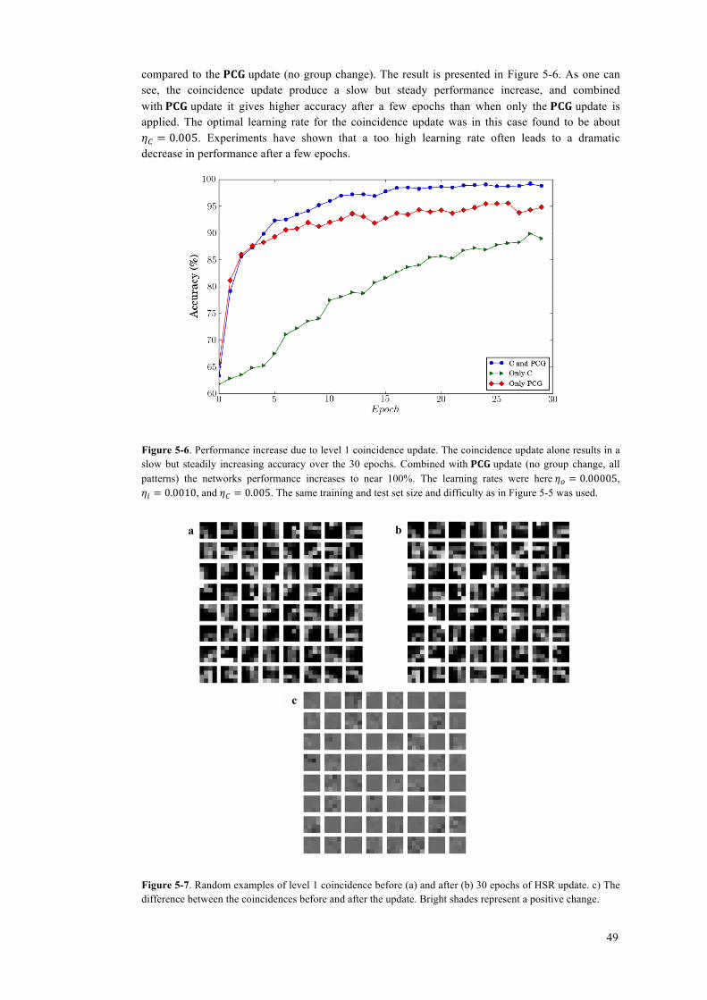
49

compared to the 𝐏𝐏𝐏𝐏𝐏𝐏 update (no group change). The result is presented in Figure 5-6. As one can see, the coincidence update produce a slow but steady performance increase, and combined with 𝐏𝐏𝐏𝐏𝐏𝐏 update it gives higher accuracy after a few epochs than when only the 𝐏𝐏𝐏𝐏𝐏𝐏 update is applied. The optimal learning rate for the coincidence update was in this case found to be about 𝜂𝜂 = 0.005. Experiments have shown that a too high learning rate often leads to a dramatic decrease in performance after a few epochs.

Figure 5-6. Performance increase due to level 1 coincidence update. The coincidence update alone results in a slow but steadily increasing accuracy over the 30 epochs. Combined with 𝐏𝐏𝐏𝐏𝐏𝐏 update (no group change, all patterns) the networks performance increases to near 100%. The learning rates were here 𝜂𝜂 = 0.00005, 𝜂𝜂 = 0.0010, and 𝜂𝜂 = 0.005. The same training and test set size and difficulty as in Figure 5-5 was used.

Figure 5-7. Random examples of level 1 coincidence before (a) and after (b) 30 epochs of HSR update. c) The difference between the coincidences before and after the update. Bright shades represent a positive change.

a b

c

50

5.7.3 HSR for discriminative fine tuning In the previously presented experiments we have investigated the efficiency of HSR as an

incremental training method for HTM. The experimental design was chosen as to simulate a situation where the training data arrives in mini-batches. However, HSR is also applicable in situations where all the training data is available from start. It then takes the role of a class supervised fine tuning algorithm which complements the initial temporally supervised training, analogous to the gradient based fine-tuning used to improve the performance of Deep Belief Nets [60].

To evaluate how much HSR is able to increase the performance of a pre-trained HTM the same training and test set difficulty as in 5.7.1 was used. A training set was generated for pre-training and then 30 epochs of HSR was applied using the same dataset. In Figure 5-8 the test set accuracy over the 30 epochs is displayed and one can see that it increases from 76.6% to 87.1%. For this experiment group change was enabled and no coincidence update was applied. In fact, experiments have shown that HSR without group change is unable to increase the performance when used for fine-tuning, and similarity the level 1 coincidence update does not seem to have any effect when applied with the same data as used for the pre-training.

Figure 5-8. HTM accuracy on 𝒮𝒮 (99,0.50,1.1,0.50,1.1,60°) as HSR is applied using the same dataset as used for pre-training. Group change was enabled, but no coincidence update was used. The experiment demonstrates that HSR not only can be used for incremental learning, but also as a supervised fine-tuning method which complements the initial temporal HTM training. The learning rates were, as above, 𝜂𝜂 =0.00005, 𝜂𝜂 = 0.0010.

5.8 Discussion & Conclusion In this chapter we propose a new algorithm for fine-tuning or incremental training of HTM. It is computationally efficient and easy to implement due to its close connection to the native belief propagation message passing in HTM.

The term 𝑄𝑄 𝑤𝑤 , the error message send from above to the output node (5.12), is the information that is propagated back through the network and lies at the heart of the algorithm. Its interpretation is not obvious: the first part, 𝑃𝑃 𝑤𝑤 |𝑒𝑒 − 𝑃𝑃 𝑤𝑤 |𝑒𝑒 , i.e., the difference between the ground truth and network posterior, is easy to understand; while the second part, − 𝑃𝑃 𝑤𝑤 |𝑒𝑒 (𝑃𝑃 𝑤𝑤 |𝑒𝑒 −𝑃𝑃 𝑤𝑤 |𝑒𝑒 ), is more mysterious. We have not been able to come up with a good interpretation of this sum yet but our hypothesis is that it arises due to the fact that we are dealing with probabilities. None of the parts can be ignored; tests have shown that they are equally important for the algorithm to produce good results.

There are some parameters to tune to find the optimal setup for a specific problem. In the experiments on incremental learning two iterations per epoch were used, and the appropriate learning rates were found therefor. With more iterations lower learning rates would likely be optimal.

51

The difference in suitable learning rate between the intermediate levels and the output level is also an important finding and can probably be explained by the fact that the 𝐏𝐏𝐏𝐏𝐏𝐏 matrix of the output node has a much more direct influence on the network posterior. The output node is also trained supervised in the pre-training while the intermediate nodes are trained unsupervised, using only time as a supervisor, this might suggest that there is more room for supervised fine-tuning in the intermediate nodes. We run some experiments where we only updated 𝐏𝐏𝐏𝐏𝐏𝐏 in the output node: in this case a small performance gain of a few percent was observed. The large improvements are thus in most part due to the refinement of the intermediate node 𝐏𝐏𝐏𝐏𝐏𝐏 matrices.

HSR can be applied with or without group change. Disabling group change leads to a much faster algorithm since many fewer derivatives need to be calculated. However, experiments show that group change is important for performance, and especially is the case where HSR is used for fine-tuning on a single training set. Neither 𝐏𝐏𝐏𝐏𝐏𝐏 update, without group change, or the level 1 coincidence update has been able to produce any performance increase in the fine-tuning case.

Several other methods can also be used to speed up the training. One approach is to only train the network with patterns that in the previous iteration were misclassified. This reduces the number of updates compared to using all patterns for every iteration. A boosting selection strategy can also be used where patterns are randomly sampled with a probability proportional to the loss generated by the pattern in the previous iteration. Experiments suggest that error selection strategy gives a few percent lower performance than selecting all patterns, while the boosting strategy lies in between selecting all patterns and only errors.

In general HSR has proven to work very well for the SDIGIT problem and the results give us reason to believe that this kind of supervised fine tuning can be extended to more difficult problems. Future work will focus on this and in general extending the HTM framework to more difficult learning problems.

52

6 Acknowledgements I would like to sincerely thank my two supervisors Prof. Davide Maltoni and Dr. Henning Sprekeler for all the help and guidance they have given me. I am very grateful to Prof. Maltoni for inviting me to work in his lab in the fall of 2011. What I learned there inspired me to explore the topic of slowness learning, and lies at the foundation of this thesis. The insights that Dr. Sprekeler has given me have also been invaluable, many thanks for taking the time to supervise me.

Many thanks also to Markus and all my other coworkers for keeping Slagkryssaren on a steady course will I have been studying. I would also like to thank Magnus, my brother, and Johannes for help with proofreading.

Last but not least, thank you Cecilia for all your support and patience.

53

7 References

[1] D. Marr, Vision: A computational investigation into the human representation and processing of visual information. WH Freeman & Company, 1982.

[2] N. Pinto, D. D. Cox, and J. J. DiCarlo, “Why is real-world visual object recognition hard?,” PLoS computational biology, vol. 4, no. 1, p. e27, Jan. 2008.

[3] G. Hinton, “Connectionist learning procedures,” Artificial intelligence, vol. 40, pp. 185–234, 1989.

[4] P. Földiák, “Learning Invariance from Transformation Sequences,” Neural Computation, vol. 3, no. 2, pp. 194–200, 1991.

[5] G. Mitchison, “Removing Time Variation with the Anti-Hebbian Differential Synapse,” Neural Computation, vol. 3, no. 3, pp. 312–320, Sep. 1991.

[6] J. Stone and A. Bray, “A learning rule for extracting spatio-temporal invariances,” Network: Computation in Neural Systems, vol. 6, no. 3, pp. 429–436, Jul. 2009.

[7] C. Kayser, W. Einhäuser, and O. Dümmer, “Extracting slow subspaces from natural videos leads to complex cells,” in In: Dorffner G, Bischoff H, Hornik K (eds) Artificial neural networks – (ICANN) LNCS 2130, Springer, Berlin Heidelberg New York, pp 1075–1080, 2001, pp. 1075–1080.

[8] L. Wiskott and T. J. Sejnowski, “Slow Feature Analysis: Unsupervised learning of invariances,” Neural computation, vol. 14, no. 4, pp. 715–770, 2002.

[9] W. Hashimoto, “Quadratic forms in natural images.,” Network (Bristol, England), vol. 14, no. 4, pp. 765–88, Nov. 2003.

[10] D. George and J. Hawkins, “Towards a mathematical theory of cortical micro-circuits.,” PLoS computational biology, vol. 5, no. 10, p. e1000532, Oct. 2009.

[11] H. Sprekeler, “On the relation of slow feature analysis and Laplacian eigenmaps.,” Neural computation, vol. 23, no. 12, pp. 3287–302, Dec. 2011.

[12] M. Belkin and P. Niyogi, “Laplacian Eigenmaps for Dimensionality Reduction and Data Representation,” Neural computation, vol. 15, no. 6, pp. 1373–1396, 2003.

[13] X. He, S. Yan, Y. Hu, and H. Zhang, “Learning a locality preserving subspace for visual recognition,” Proceedings Ninth IEEE International Conference on Computer Vision, vol. 1, pp. 385–392, 2003.

[14] Y. LeCun and L. Bottou, “Learning methods for generic object recognition with invariance to pose and lighting,” in Proceedings of the 2004 IEEE Computer Society Conference on Computer Vision and Pattern Recognition, 2004. CVPR 2004., vol. 2, pp. 97–104.

[15] A. Coates, H. Lee, and A. Y. Ng, “An Analysis of Single-Layer Networks in Unsupervised Feature Learning,” AISTATS, 2011.

[16] P. Berkes and L. Wiskott, “Slow feature analysis yields a rich repertoire of complex cell properties.,” Journal of vision, vol. 5, no. 6, pp. 579–602, Jan. 2005.

[17] R. Hadsell, S. Chopra, and Y. LeCun, “Dimensionality Reduction by Learning an Invariant Mapping,” 2006 IEEE Computer Society Conference on Computer Vision and Pattern Recognition - Volume 2 (CVPR’06), vol. 2, pp. 1735–1742, 2006.

54

[18] A. N. Escalante-B. and L. Wiskott, “Heuristic Evaluation of Expansions for Non-linear Hierarchical Slow Feature Analysis,” 2011 10th International Conference on Machine Learning and Applications and Workshops, no. 10, pp. 133–138, Dec. 2011.

[19] A. Bray and D. Martinez, “Kernel-based Extraction of Slow Features: Complex Cells Learn Disparity and Translation Invariance from Natural Images,” Advances in Neural Information Processing Systems, vol. 15, 2002.

[20] W. Böhmer, S. Grünewälder, H. Nickisch, and K. Obermayer, “Regularized sparse kernel slow feature analysis,” Machine Learning and Knowledge Discovery in Databases Lecture Notes in Computer Science, vol. 6911, pp. 235–248, 2011.

[21] R. Turner and M. Sahani, “A Maximum-Likelihood Interpretation for Slow Feature Analysis,” Neural Computation, vol. 19, no. 4, pp. 1022–1038, 2007.

[22] A. Hyvärinen and E. Oja, “Independent component analysis: algorithms and applications.,” Neural networks  : the official journal of the International Neural Network Society, vol. 13, no. 4–5, pp. 411–30, 2000.

[23] T. Blaschke, P. Berkes, and L. Wiskott, “What is the relation between slow feature analysis and independent component analysis?,” Neural computation, vol. 18, no. 10, pp. 2495–508, Oct. 2006.

[24] L. Lovász, “Random walks on graphs: A survey,” Combinatorics, Paul erdos is eighty, vol. 2, 1993.

[25] U. Luxburg, “A tutorial on spectral clustering,” Statistics and Computing, vol. 17, no. 4, pp. 395–416, Aug. 2007.

[26] J. Shi and J. Malik, “Normalized cuts and image segmentation,” IEEE Transactions on Pattern Analysis and Machine Intelligence, vol. 22, no. 8, pp. 888–905, 2000.

[27] B. Nadler and M. Galun, “Fundamental limitations of spectral clustering,” Advances in Neural Information Processing Systems, vol. 19, pp. 1017–1024, 2007.

[28] Y. Bengio and J. Paiement, “Out-of-Sample Extensions for LLE, Isomap, MDS, Eigenmaps, and Spectral Clustering,” In Advances in Neural Information Processing Systems, 2003.

[29] M. Franzius, N. Wilbert, and L. Wiskott, “Invariant object recognition and pose estimation with slow feature analysis,” Neural computation, vol. 2323, pp. 2289–2323, 2011.

[30] S. J. Kiebel, J. Daunizeau, and K. J. Friston, “A hierarchy of time-scales and the brain.,” PLoS computational biology, vol. 4, no. 11, p. e1000209, Nov. 2008.

[31] U. Hasson, E. Yang, I. Vallines, D. J. Heeger, and N. Rubin, “A hierarchy of temporal receptive windows in human cortex.,” The Journal of neuroscience  : the official journal of the Society for Neuroscience, vol. 28, no. 10, pp. 2539–50, Mar. 2008.

[32] P. Niyogi, “Locality preserving projections,” Advances in neural information processing systems, 2004.

[33] F. R. Gantmacher, Matrix Theory, vol. 1. AMS Chelsea Publishing., 1959.

[34] X. He, S. Yan, Y. Hu, P. Niyogi, and H.-J. Zhang, “Face recognition using laplacianfaces.,” IEEE transactions on pattern analysis and machine intelligence, vol. 27, no. 3, pp. 328–40, Mar. 2005.

55

[35] X. Chen, J. Zhang, and D. Li, “Direct Discriminant Locality Preserving Projection with Hammerstein Polynomial Expansion,” IEEE transactions on image processing  : a publication of the IEEE Signal Processing Society, vol. 21, no. 12, pp. 4858–67, Dec. 2012.

[36] P. Berkes, “Pattern recognition with slow feature analysis,” CogPrints, 2005.

[37] P. Berkes, “Handwritten digit recognition with nonlinear fisher discriminant analysis,” Artificial Neural Networks: Formal Models and Their Applications – ICANN 2005 Lecture Notes in Computer Science, vol. 3697, pp. 285–287, 2005.

[38] S. Klampfl and W. Maass, “A theoretical basis for emergent pattern discrimination in neural systems through slow feature extraction.,” Neural computation, vol. 22, no. 12, pp. 2979–3035, Dec. 2010.

[39] J. J. DiCarlo and D. D. Cox, “Untangling invariant object recognition.,” Trends in cognitive sciences, vol. 11, no. 8, pp. 333–341, Aug. 2007.

[40] M. Belkin, P. Niyogi, and V. Sindhwani, “Manifold regularization: A geometric framework for learning from labeled and unlabeled examples,” The Journal of Machine Learning Research, vol. 7, pp. 2399–2434, 2006.

[41] J. B. Tenenbaum, V. de Silva, and J. C. Langford, “A global geometric framework for nonlinear dimensionality reduction.,” Science (New York, N.Y.), vol. 290, no. 5500, pp. 2319–23, Dec. 2000.

[42] S. T. Roweis and L. K. Saul, “Nonlinear dimensionality reduction by locally linear embedding.,” Science (New York, N.Y.), vol. 290, no. 5500, pp. 2323–6, Dec. 2000.

[43] S. Yan, D. Xu, B. Zhang, H.-J. Zhang, Q. Yang, and S. Lin, “Graph embedding and extensions: a general framework for dimensionality reduction.,” IEEE transactions on pattern analysis and machine intelligence, vol. 29, no. 1, pp. 40–51, Jan. 2007.

[44] D. Cai, X. He, and J. Han, “Semi-supervised Discriminant Analysis,” 2007 IEEE 11th International Conference on Computer Vision, 2007.

[45] D. Maltoni, “Pattern Recognition by Hierarchical Temporal Memory,” DEIS TR, 2011. [Online]. Available: http://bias.csr.unibo.it/maltoni/HTM_TR_v1.0.pdf.

[46] A. Krizhevsky and G. Hinton, “Learning multiple layers of features from tiny images,” Master Thesis, 2009.

[47] Y. LeCun, B. Boser, J. S. J. Denker, D. Henderson, R. E. Howard, W. Hubbard, and L. D. Jackel, “Backpropagation Applied to Handwritten Zip Code Recognition,” Neural Computation, vol. 1, no. 4, pp. 541–551, Dec. 1989.

[48] V. Nair and G. Hinton, “3D Object Recognition with Deep Belief Nets,” Advances in Neural Information Processing Systems 22, 2009.

[49] R. Uetz and S. Behnke, “Large-scale object recognition with CUDA-accelerated hierarchical neural networks,” In Intelligent Computing and Intelligent Systems, vol. 1, pp. 536–541, 2009.

[50] T. Zito, N. Wilbert, L. Wiskott, and P. Berkes, “Modular Toolkit for Data Processing (MDP): A Python Data Processing Framework.,” Frontiers in neuroinformatics, vol. 2, p. 8, Jan. 2008.

[51] F. Pedregosa, G. Varoquaux, A. Gramfort, V. Michel, B. Thirion, O. Grisel, M. Blondel, P. Prettenhofer, R. Weiss, V. Dubourg, J. Vanderplas, A. Passos, D. Cournapeau, M. Brucher,

56

M. Perrot, and É. Duchesnay, “Scikit-learn: Machine Learning in Python,” The Journal of Machine Learning Research, vol. 12, pp. 2825–2830, Nov. 2011.

[52] D. Arthur, “k-means++  : The Advantages of Careful Seeding,” SODA ’07 Proceedings of the eighteenth annual ACM-SIAM symposium on Discrete algorithms, pp. 1027 – 1035.

[53] D. Sculley, “Web-scale k-means clustering,” Proceedings of the 19th international conference on World wide web - WWW ’10, p. 1177, 2010.

[54] C.-C. Chang and C.-J. Lin, “LIBSVM,” ACM Transactions on Intelligent Systems and Technology, vol. 2, no. 3, pp. 1–27, Apr. 2011.

[55] D. George, “How the Brain Might Work: A Hierarchical and Temporal Model for Learning and Recognition,” Stanford University, 2008.

[56] T. S. Lee and D. Mumford, “Hierarchical Bayesian inference in the visual cortex,” J. Opt. Soc. Am, vol. 20, no. 7, pp. 1434–1448, 2003.

[57] M. Ranzato, F. J. Huang, Y.-L. Boureau, and Y. LeCun, “Unsupervised Learning of Invariant Feature Hierarchies with Applications to Object Recognition,” 2007 IEEE Conference on Computer Vision and Pattern Recognition, pp. 1–8, Jun. 2007.

[58] J. Pearl, Probabilistic Reasoning in Intelligent Systems. Morgan-Kaufmann, 1988.

[59] R. Jin, C. Ding, and F. Kang, “A Probabilistic Approach for Optimizing Spectral Clustering,” In Advances in Neural Information Processing Systems 18, 2005.

[60] Y. Bengio, “Learning Deep Architectures for AI,” Foundations and Trends in Machine Learning, vol. 2, no. 1, pp. 1–127, 2009.

[61] V. Vapnik, Statistical learning theory. Wiley-Interscience, 1989.

[62] D. Maltoni and E. M. Rehn, “Incremental Learning by Message Passing in Hierarchical Temporal Memory,” DEIS TR, 2012. [Online]. Available: http://bias.csr.unibo.it/maltoni/HTM_HSR_TR_v1.0.p.

57

Appendix A Here the equivalence between the MaxStab objective of [45] and the Ncut objective [26] is derived. However, notice that even though the objectives are the same MaxStab also impose hard limits on the maximum and minimum cluster size. For a two cluster case Ncut is:

𝑁𝑁𝑁𝑁𝑁𝑁𝑁𝑁 𝑔𝑔 ,𝑔𝑔 = 𝑚𝑚𝑚𝑚𝑚𝑚𝑐𝑐𝑐𝑐𝑐𝑐 𝑔𝑔 ,𝑔𝑔𝑣𝑣𝑣𝑣𝑣𝑣 𝑔𝑔

+𝑐𝑐𝑐𝑐𝑐𝑐 𝑔𝑔 ,𝑔𝑔𝑣𝑣𝑣𝑣𝑣𝑣 𝑔𝑔

= 𝑚𝑚𝑚𝑚𝑚𝑚 𝑃𝑃 𝑐𝑐 ∈ 𝑔𝑔 |𝑐𝑐 ∈ 𝑔𝑔 + 𝑃𝑃 𝑐𝑐 ∈ 𝑔𝑔 |𝑐𝑐 ∈ 𝑔𝑔

Ncut is therefore minimizing the probability that we walk from one cluster to the other. This is equivalent to maximizing the probability of staying in the same cluster:

𝑁𝑁𝑁𝑁𝑁𝑁𝑁𝑁 𝑔𝑔 ,𝑔𝑔 …𝑔𝑔 = 𝑚𝑚𝑚𝑚𝑚𝑚𝑐𝑐𝑐𝑐𝑐𝑐(𝑔𝑔 ,𝑔𝑔 )𝑣𝑣𝑣𝑣𝑣𝑣(𝑔𝑔 )

= 𝑚𝑚𝑚𝑚𝑚𝑚𝑐𝑐𝑐𝑐𝑐𝑐(𝑔𝑔 ,𝑔𝑔 )𝑣𝑣𝑣𝑣𝑣𝑣(𝑔𝑔 )

= 𝑚𝑚𝑚𝑚𝑚𝑚𝑎𝑎𝑎𝑎𝑎𝑎𝑎𝑎𝑎𝑎(𝑔𝑔 ,𝑔𝑔 )𝑣𝑣𝑣𝑣𝑣𝑣(𝑔𝑔 )

where 𝑐𝑐𝑐𝑐𝑐𝑐 𝑔𝑔 ,𝑔𝑔 = 𝑎𝑎𝑎𝑎𝑎𝑎𝑎𝑎𝑎𝑎(𝑔𝑔 ,𝑔𝑔 ). This relationship between maximizing and minimizing the Ncut or “Nassoc” objective has been shown by Shi & Malik, 2000 [26].

On the other hand, MaxStab has the following objective:

𝑀𝑀𝑀𝑀𝑀𝑀𝑀𝑀𝑀𝑀𝑀𝑀𝑀𝑀 𝑔𝑔 ,𝑔𝑔 …𝑔𝑔 = 𝑚𝑚𝑚𝑚𝑚𝑚1𝑛𝑛

𝑃𝑃 𝑐𝑐 𝑐𝑐∈∈ 𝑃𝑃 𝑐𝑐 𝑃𝑃 c∈

= 𝑚𝑚𝑚𝑚𝑚𝑚1𝑛𝑛

𝑤𝑤𝑑𝑑∈∈

𝑑𝑑𝑣𝑣𝑣𝑣𝑣𝑣(𝐶𝐶)

𝑑𝑑𝑣𝑣𝑣𝑣𝑣𝑣(𝐶𝐶)∈

= 𝑚𝑚𝑚𝑚𝑚𝑚1𝑛𝑛

𝑤𝑤∈∈

𝑣𝑣𝑣𝑣𝑣𝑣(𝑔𝑔 )= 𝑚𝑚𝑚𝑚𝑚𝑚

1𝑛𝑛

𝑎𝑎𝑎𝑎𝑎𝑎𝑎𝑎𝑎𝑎(𝑔𝑔 ,𝑔𝑔 )𝑣𝑣𝑣𝑣𝑣𝑣(𝑔𝑔 )

which is equivalent to the Ncut/Nassoc objective given a fixed number of groups/clusters. The relation between random walks on graphs and Markov chains has been used here (equation (2.7) and (2.8)). Moreover, the stability of a group can be defined as its normalized inner association:

𝑠𝑠𝑠𝑠𝑠𝑠𝑠𝑠𝑠𝑠𝑠𝑠𝑠𝑠𝑠𝑠𝑠𝑠 𝑔𝑔 =𝑎𝑎𝑎𝑎𝑎𝑎𝑎𝑎𝑎𝑎(𝑔𝑔 ,𝑔𝑔 )𝑣𝑣𝑣𝑣𝑣𝑣(𝑔𝑔 )

58

Appendix B Here we derive the coincidence update rule for level 𝐿𝐿 in a four-level HTM. Let ℎ be a node

in level 𝐿𝐿 and 𝑑𝑑 a node in 𝐿𝐿 . We want to find −𝒄𝒄( )[ ]

where 𝒄𝒄( )[𝑞𝑞] is the 𝑞𝑞: 𝑡𝑡ℎ

element of coincidence 𝑝𝑝 in node 𝑑𝑑. For more details on the notation, see the Appendix of [62].

𝐿𝐿(𝑒𝑒 , 𝑒𝑒 ) =12

𝑃𝑃 𝑤𝑤 |𝑒𝑒 − 𝑃𝑃 𝑤𝑤 |𝑒𝑒

−𝜕𝜕𝜕𝜕

𝜕𝜕𝒄𝒄( )[𝑞𝑞]= 𝑃𝑃 𝑤𝑤 |𝑒𝑒 − 𝑃𝑃 𝑤𝑤 |𝑒𝑒

𝜕𝜕𝜕𝜕 𝑤𝑤 |𝑒𝑒

𝜕𝜕𝒄𝒄( )[𝑞𝑞] (1)

Following the same steps leading to equation (23) in Appendix B of [62], we obtain:

−𝜕𝜕𝜕𝜕

𝜕𝜕𝒄𝒄( )[𝑞𝑞]=

𝜕𝜕𝐲𝐲[𝑗𝑗]

𝜕𝜕𝒄𝒄( )[𝑞𝑞]𝑃𝑃𝑃𝑃𝑃𝑃 ∙ 𝑄𝑄(𝑤𝑤 ) (2)

We then expand all derivatives:

𝜕𝜕𝐲𝐲 𝑗𝑗

𝜕𝜕𝒄𝒄 𝑞𝑞= 𝐲𝐲 𝑗𝑗 ∙

𝜕𝜕𝜕𝜕𝒄𝒄 𝑞𝑞

𝛌𝛌 𝐜𝐜 𝑟𝑟

𝛌𝛌 𝐜𝐜 𝑟𝑟=

𝐲𝐲 𝑗𝑗

𝛌𝛌 𝐜𝐜 ℎ∙𝜕𝜕𝛌𝛌 𝐜𝐜 ℎ

𝜕𝜕𝒄𝒄 𝑞𝑞

𝜕𝜕𝛌𝛌 𝐜𝐜 ℎ

𝜕𝜕𝒄𝒄( )[𝑞𝑞]=

𝜕𝜕

𝜕𝜕𝒄𝒄( )[𝑞𝑞]𝑃𝑃𝑃𝑃𝑃𝑃 𝐜𝐜 [ ]

( ) ∙ 𝐲𝐲( )[𝑡𝑡]

( )

= 𝑃𝑃𝑃𝑃𝑃𝑃 𝐜𝐜 [ ]( ) ∙

𝜕𝜕𝐲𝐲( )[𝑡𝑡]

𝜕𝜕𝒄𝒄( )[𝑞𝑞]

( )

𝜕𝜕𝐲𝐲( )[𝑡𝑡]

𝜕𝜕𝒄𝒄( )[𝑞𝑞]= 𝐲𝐲( )[𝑡𝑡] ∙

𝜕𝜕𝜕𝜕𝒄𝒄( )[𝑞𝑞]

𝛌𝛌 𝐜𝐜( )[𝑠𝑠]

𝛌𝛌( ) 𝐜𝐜( )[𝑠𝑠]

( )

=𝐲𝐲( )[𝑡𝑡]

𝛌𝛌( ) 𝐜𝐜( )[𝑑𝑑]∙𝜕𝜕𝛌𝛌 𝐜𝐜( )[𝑑𝑑]

𝜕𝜕𝒄𝒄( )[𝑞𝑞]

𝜕𝜕𝛌𝛌 𝐜𝐜( )[𝑑𝑑]

𝜕𝜕𝒄𝒄( )[𝑞𝑞]= 𝑃𝑃𝑃𝑃𝑃𝑃

𝐜𝐜( )[ ]( ) ∙

𝜕𝜕𝐲𝐲( )[𝑣𝑣]

𝜕𝜕𝒄𝒄( )[𝑞𝑞]

( )

= 𝑃𝑃𝑃𝑃𝑃𝑃 𝐜𝐜( )[ ]( ) ∙

𝜕𝜕𝐲𝐲( )[𝑝𝑝]

𝜕𝜕𝒄𝒄( )[𝑞𝑞]

𝜕𝜕𝐲𝐲 𝑝𝑝

𝜕𝜕𝒄𝒄 𝑞𝑞=

𝜕𝜕

𝜕𝜕𝒄𝒄 𝑞𝑞𝑒𝑒− 𝒄𝒄 − 𝛌𝛌 𝜎𝜎 =

2 ∙ (𝛌𝛌 [𝑞𝑞] − 𝒄𝒄( )[𝑞𝑞])𝜎𝜎

∙ 𝐲𝐲( )[𝑝𝑝]

where 𝛌𝛌 [𝑞𝑞] is the input message/image to node 𝑑𝑑 from input node 𝑞𝑞. We then reinsert everything into (2):

−𝜕𝜕𝜕𝜕

𝜕𝜕𝒄𝒄( )[𝑞𝑞]=

𝐲𝐲 𝑗𝑗

𝛌𝛌 𝐜𝐜 ℎ𝑃𝑃𝑃𝑃𝑃𝑃 𝐜𝐜 [ ]

( ) ∙𝐲𝐲( )[𝑡𝑡]

𝛌𝛌( ) 𝐜𝐜( )[𝑑𝑑]𝑃𝑃𝑃𝑃𝑃𝑃

𝐜𝐜( )[ ]

( )

( )

2 ∙ (𝛌𝛌 [𝑞𝑞] − 𝒄𝒄( )[𝑞𝑞])𝜎𝜎 ∙ 𝐲𝐲( ) 𝑝𝑝 ∙ 𝑃𝑃𝑃𝑃𝑃𝑃 ∙ 𝑄𝑄(𝑤𝑤 )

=2 ∙ (𝛌𝛌 [𝑞𝑞] − 𝒄𝒄( )[𝑞𝑞])

𝜎𝜎 ∙ 𝐲𝐲( ) 𝑝𝑝 ∙𝐲𝐲( )[𝑡𝑡]


𝐜𝐜( )[ ]

( )

( )

∙𝐲𝐲 𝑗𝑗

𝛌𝛌 𝐜𝐜 ℎ∙ 𝑃𝑃𝑃𝑃𝑃𝑃 𝐜𝐜 ∙ 𝑃𝑃𝑃𝑃𝑃𝑃 ∙ 𝑄𝑄(𝑤𝑤 )

=2 ∙ (𝛌𝛌 [𝑞𝑞] − 𝒄𝒄( )[𝑞𝑞])

𝜎𝜎 ∙ 𝐲𝐲( ) 𝑝𝑝𝐲𝐲( )[𝑡𝑡]


𝐜𝐜( )[ ]

( )

( )

𝐼𝐼𝐜𝐜 𝐠𝐠( ) 𝐲𝐲 𝑗𝑗𝛌𝛌 𝑓𝑓

∙ 𝑃𝑃𝑃𝑃𝑃𝑃 ∙ 𝑃𝑃𝑃𝑃𝑃𝑃 ∙ 𝑄𝑄(𝑤𝑤 )

( )

(3)

59

Here we are reversing this tick from Appendix C of [62]: “Instead of summing over all groups in ℎ and check if 𝐼𝐼𝐜𝐜 𝐠𝐠( ) = 1 , we can set 𝑓𝑓 = 𝐜𝐜 ℎ (only one group in ℎ is part of 𝐜𝐜 )”, to get a sum

over the groups in ℎ.

Given that the top-down error message to node ℎ is:

𝛑𝛑( )[𝑓𝑓] = 𝐼𝐼𝐜𝐜 𝐠𝐠 ∙ 𝐲𝐲[𝑗𝑗] ∙ 𝑃𝑃𝑃𝑃𝑃𝑃 ∙ 𝑄𝑄 𝑤𝑤

and

𝐁𝐁𝐁𝐁𝐁𝐁( )[𝐜𝐜( )] = 𝐲𝐲( )[𝑡𝑡] ∙𝑃𝑃𝑃𝑃𝑃𝑃

𝛌𝛌 𝑓𝑓∙ 𝛑𝛑( )[𝑓𝑓]

( )

Equation 3 can be rewritten as

−𝜕𝜕𝜕𝜕

𝜕𝜕𝒄𝒄( )[𝑞𝑞]=2 ∙ (𝛌𝛌 [𝑞𝑞] − 𝒄𝒄( )[𝑞𝑞])

𝜎𝜎∙ 𝐲𝐲( ) 𝑝𝑝

∙𝑃𝑃𝑃𝑃𝑃𝑃

𝐜𝐜( )[ ]( )

𝛌𝛌( ) 𝐜𝐜( )[𝑑𝑑]∙ 𝐲𝐲( )[𝑡𝑡]

( )

𝑃𝑃𝑃𝑃𝑃𝑃

𝛌𝛌 𝑓𝑓∙ 𝛑𝛑( )[𝑓𝑓]

( )

=2 ∙ (𝛌𝛌 [𝑞𝑞] − 𝒄𝒄( )[𝑞𝑞])

𝜎𝜎∙ 𝐲𝐲( ) 𝑝𝑝 ∙

𝑃𝑃𝑃𝑃𝑃𝑃 𝐜𝐜( )[ ]( )

𝛌𝛌( ) 𝐜𝐜( )[𝑑𝑑]∙ 𝐁𝐁𝐁𝐁𝐁𝐁( )[𝐜𝐜( )]

( )

=2 ∙ (𝛌𝛌 [𝑞𝑞] − 𝒄𝒄( )[𝑞𝑞])

𝜎𝜎∙ 𝐲𝐲( ) 𝑝𝑝 ∙ 𝐼𝐼𝐜𝐜 𝐠𝐠( ) ∙

𝑃𝑃𝑃𝑃𝑃𝑃 ( )

𝛌𝛌( ) 𝑘𝑘∙ 𝐁𝐁𝐁𝐁𝐁𝐁( )[𝐜𝐜( )]

( )( )

(4)

Here we use the “sum over groups”-trick again. Equation (4) can be simplified further by noting that

𝛑𝛑( ) 𝑘𝑘 = 𝐼𝐼𝐜𝐜( ) 𝐠𝐠 ∙ 𝐁𝐁𝐁𝐁𝐁𝐁( )[𝐜𝐜( )]

Equation (4) is then

−𝜕𝜕𝜕𝜕

𝜕𝜕𝒄𝒄( )[𝑞𝑞]=2 ∙ (𝛌𝛌 [𝑞𝑞] − 𝒄𝒄( )[𝑞𝑞])

𝜎𝜎∙ 𝐲𝐲( ) 𝑝𝑝 ∙

𝑃𝑃𝑃𝑃𝑃𝑃 ( )

𝛌𝛌( ) 𝑘𝑘∙ 𝛑𝛑( )[𝑘𝑘]

( )

=2 ∙ (𝛌𝛌 [𝑞𝑞] − 𝒄𝒄( )[𝑞𝑞])

𝜎𝜎∙ 𝐁𝐁𝐁𝐁𝐁𝐁( )[𝐜𝐜( )]

QED.

On the Slowness Principle and Learning in Hierarchical Temporal Memory

Documents

Transcript of On the Slowness Principle and Learning in Hierarchical Temporal Memory