On the Shoulders of Giants A Course in Single Variable Calculus - Smith & Mcleland.pdf
291
Transcript of On the Shoulders of Giants A Course in Single Variable Calculus - Smith & Mcleland.pdf


CONTENTS
Preface v
1 Terror, tragedy and bad vibrations 11.1 Introduction . . . . . . . . . . . . . . . . . . . . . . . . . . . . . . . . . . . . . . . 11.2 The Tower of Terror . . . . . . . . . . . . . . . . . . . . . . . . . . . . . . . . . . 11.3 Into thin air . . . . . . . . . . . . . . . . . . . . . . . . . . . . . . . . . . . . . . . 41.4 Music and the bridge . . . . . . . . . . . . . . . . . . . . . . . . . . . . . . . . . . 71.5 Discussion . . . . . . . . . . . . . . . . . . . . . . . . . . . . . . . . . . . . . . . . 81.6 Rules of calculation . . . . . . . . . . . . . . . . . . . . . . . . . . . . . . . . . . . 9
2 Functions 112.1 Rules of calculation . . . . . . . . . . . . . . . . . . . . . . . . . . . . . . . . . . . 112.2 Intervals on the real line . . . . . . . . . . . . . . . . . . . . . . . . . . . . . . . . . 152.3 Graphs of functions . . . . . . . . . . . . . . . . . . . . . . . . . . . . . . . . . . . 172.4 Examples of functions . . . . . . . . . . . . . . . . . . . . . . . . . . . . . . . . . 20
3 Continuity and smoothness 273.1 Smooth functions . . . . . . . . . . . . . . . . . . . . . . . . . . . . . . . . . . . . 273.2 Continuity . . . . . . . . . . . . . . . . . . . . . . . . . . . . . . . . . . . . . . . . 30
4 Differentiation 414.1 The derivative . . . . . . . . . . . . . . . . . . . . . . . . . . . . . . . . . . . . . . 414.2 Rules for differentiation . . . . . . . . . . . . . . . . . . . . . . . . . . . . . . . . . 484.3 Velocity, acceleration and rates of change . . . . . . . . . . . . . . . . . . . . . . . 53
5 Falling bodies 575.1 The Tower of Terror . . . . . . . . . . . . . . . . . . . . . . . . . . . . . . . . . . 575.2 Solving differential equations . . . . . . . . . . . . . . . . . . . . . . . . . . . . . . 625.3 General remarks . . . . . . . . . . . . . . . . . . . . . . . . . . . . . . . . . . . . . 655.4 Increasing and decreasing functions . . . . . . . . . . . . . . . . . . . . . . . . . . 685.5 Extreme values . . . . . . . . . . . . . . . . . . . . . . . . . . . . . . . . . . . . . 70
6 Series and the exponential function 756.1 The air pressure problem . . . . . . . . . . . . . . . . . . . . . . . . . . . . . . . . 756.2 Infinite series . . . . . . . . . . . . . . . . . . . . . . . . . . . . . . . . . . . . . . 816.3 Convergence of series . . . . . . . . . . . . . . . . . . . . . . . . . . . . . . . . . . 846.4 Radius of convergence . . . . . . . . . . . . . . . . . . . . . . . . . . . . . . . . . 90
TLFeBOOK

ii CONTENTS
6.5 Differentiation of power series . . . . . . . . . . . . . . . . . . . . . . . . . . . . . 936.6 The chain rule . . . . . . . . . . . . . . . . . . . . . . . . . . . . . . . . . . . . . . 966.7 Properties of the exponential function . . . . . . . . . . . . . . . . . . . . . . . . . 996.8 Solution of the air pressure problem . . . . . . . . . . . . . . . . . . . . . . . . . . 102
7 Trigonometric functions 1097.1 Vibrating strings and cables . . . . . . . . . . . . . . . . . . . . . . . . . . . . . . . 1097.2 Trigonometric functions . . . . . . . . . . . . . . . . . . . . . . . . . . . . . . . . 1117.3 More on the sine and cosine functions . . . . . . . . . . . . . . . . . . . . . . . . . 1147.4 Triangles, circles and the number � . . . . . . . . . . . . . . . . . . . . . . . . . . . 1197.5 Exact values of the sine and cosine functions . . . . . . . . . . . . . . . . . . . . . . 1227.6 Other trigonometric functions . . . . . . . . . . . . . . . . . . . . . . . . . . . . . . 125
8 Oscillation problems 1278.1 Second order linear differential equations . . . . . . . . . . . . . . . . . . . . . . . 1278.2 Complex numbers . . . . . . . . . . . . . . . . . . . . . . . . . . . . . . . . . . . . 1348.3 Complex series . . . . . . . . . . . . . . . . . . . . . . . . . . . . . . . . . . . . . 1408.4 Complex roots of the auxiliary equation . . . . . . . . . . . . . . . . . . . . . . . . 1438.5 Simple harmonic motion and damping . . . . . . . . . . . . . . . . . . . . . . . . . 1458.6 Forced oscillations . . . . . . . . . . . . . . . . . . . . . . . . . . . . . . . . . . . 153
9 Integration 1679.1 Another problem on the Tower of Terror . . . . . . . . . . . . . . . . . . . . . . . . 1679.2 More on air pressure . . . . . . . . . . . . . . . . . . . . . . . . . . . . . . . . . . 1689.3 Integrals and primitive functions . . . . . . . . . . . . . . . . . . . . . . . . . . . . 1709.4 Areas under curves . . . . . . . . . . . . . . . . . . . . . . . . . . . . . . . . . . . 1719.5 Area functions . . . . . . . . . . . . . . . . . . . . . . . . . . . . . . . . . . . . . . 1749.6 Integration . . . . . . . . . . . . . . . . . . . . . . . . . . . . . . . . . . . . . . . . 1769.7 Evaluation of integrals . . . . . . . . . . . . . . . . . . . . . . . . . . . . . . . . . 1829.8 The fundamental theorem of the calculus . . . . . . . . . . . . . . . . . . . . . . . . 1879.9 The logarithm function . . . . . . . . . . . . . . . . . . . . . . . . . . . . . . . . . 188
10 Inverse functions 19710.1 The existence of inverses . . . . . . . . . . . . . . . . . . . . . . . . . . . . . . . . 20010.2 Calculating function values for inverses . . . . . . . . . . . . . . . . . . . . . . . . 20510.3 The oscillation problem again . . . . . . . . . . . . . . . . . . . . . . . . . . . . . 21410.4 Inverse trigonometric functions . . . . . . . . . . . . . . . . . . . . . . . . . . . . . 21810.5 Other inverse trigonometric functions . . . . . . . . . . . . . . . . . . . . . . . . . 221
11 Hyperbolic functions 22511.1 Hyperbolic functions . . . . . . . . . . . . . . . . . . . . . . . . . . . . . . . . . . 22511.2 Properties of the hyperbolic functions . . . . . . . . . . . . . . . . . . . . . . . . . 22711.3 Inverse hyperbolic functions . . . . . . . . . . . . . . . . . . . . . . . . . . . . . . 230

CONTENTS iii
12 Methods of integration 23512.1 Introduction . . . . . . . . . . . . . . . . . . . . . . . . . . . . . . . . . . . . . . . 23512.2 Calculation of definite integrals . . . . . . . . . . . . . . . . . . . . . . . . . . . . . 23712.3 Integration by substitution . . . . . . . . . . . . . . . . . . . . . . . . . . . . . . . 23912.4 Integration by parts . . . . . . . . . . . . . . . . . . . . . . . . . . . . . . . . . . . 24112.5 The method of partial fractions . . . . . . . . . . . . . . . . . . . . . . . . . . . . . 24312.6 Integrals with a quadratic denominator . . . . . . . . . . . . . . . . . . . . . . . . . 24712.7 Concluding remarks . . . . . . . . . . . . . . . . . . . . . . . . . . . . . . . . . . . 249
13 A nonlinear differential equation 25113.1 The energy equation . . . . . . . . . . . . . . . . . . . . . . . . . . . . . . . . . . 25213.2 Conclusion . . . . . . . . . . . . . . . . . . . . . . . . . . . . . . . . . . . . . . . 259
Answers 261
Index 281

This page intentionally left blank
PREFACE
If I have seen further it is by standing on the shoulders of Giants.Sir Isaac Newton, 1675.
This book presents an innovative treatment of single variable calculus designed as an introductorymathematics textbook for engineering and science students. The subject material is developed bymodelling physical problems, some of which would normally be encountered by students as experi-ments in a first year physics course. The solutions of these problems provide a means of introducingmathematical concepts as they are needed. The book presents all of the material from a traditional firstyear calculus course, but it will appear for different purposes and in a different order from standardtreatments.
The rationale of the book is that the mathematics should be introduced in a context tailored to theneeds of the audience. Each mathematical concept is introduced only when it is needed to solve aparticular practical problem, so at all stages, the student should be able to connect the mathematicalconcept with a particular physical idea or problem. For various reasons, notions such as relevanceor just in time mathematics are common catchcries. We have responded to these in a way whichmaintains the professional integrity of the courses we teach.
The book begins with a collection of problems. A discussion of these problems leads to the ideaof a function, which in the first instance will be regarded as a rule for numerical calculation. In somecases, real or hypothetical results will be presented, from which the function can be deduced. Partof the purpose of the book is to assist students in learning how to define the rules for calculatingfunctions and to understand why such rules are needed. The most common way of expressing a rule isby means of an algebraic formula and this is the way in which most students first encounter functions.Unfortunately, many of them are unable to progress beyond the functions as formulas concept. Ourstance in this book is that functions are rules for numerical calculation and so must be presentedin a form which allows function values to be calculated in decimal form to an arbitrary degree ofaccuracy. For this reason, trigonometric functions first appear as power series solutions to differentialequations, rather than through the common definitions in terms of triangles. The latter definitionsmay be intuitively simpler, but they are of little use in calculating function values or preparing thestudent for later work. We begin with simple functions defined by algebraic formulas and move on tofunctions defined by power series and integrals. As we progress through the book, different physicalproblems give rise to various functions and if the calculation of function values requires the numericalevaluation of an integral, then this simply has to be accepted as an inconvenient but unavoidableproperty of the problem. We would like students to appreciate the fact that some problems, such asthe nonlinear pendulum, require sophisticated mathematical methods for their analysis and difficultmathematics is unavoidable if we wish to solve the problem. It is not introduced simply to provide an

vi PREFACE
intellectual challenge or to filter out the weaker students.Our attitude to proofs and rigour is that we believe that all results should be correctly stated, but
not all of them need formal proof. Most of all, we do not believe that students should be presentedwith handwaving arguments masquerading as proofs. If we feel that a proof is accessible and thatthere is something useful to be learned from the proof, then we provide it. Otherwise, we state theresult and move on. Students are quite capable of using the results on term-by-term differentiation ofa power series for instance, even if they have not seen the proof. However, we think that it is importantto emphasise that a power series can be differentiated in this way only within the interior of its intervalof convergence. By this means we can take the applications in this book beyond the artificial examplesoften seen in standard texts.
We discuss continuity and differentiation in terms of convergence of sequences. We think that thisis intuitively more accessible than the usual approach of considering limits of functions. If limits aretreated with the full rigour of the � -
�approach, then they are too difficult for the average beginning
student, while a non-rigorous treatment simply leads to confusion.The remainder of this preface summarises the content of this book. Our list of physical problems
includes the vertical motion of a projectile, the variation of atmospheric pressure with height, the mo-tion of a body in simple harmonic motion, underdamped and overdamped oscillations, forced dampedoscillations and the nonlinear pendulum. In each case the solution is a function which relates two vari-ables. An appeal to the student’s physical intuition suggests that the graphs of these functions shouldhave certain properties. Closer analysis of these intuitive ideas leads to the concepts of continuity anddifferentiability. Modelling the problems leads to differential equations for the desired functions andin solving these equations we discuss power series, radius of convergence and term-by-term differen-tiation. In discussing oscillation we have to consider the case where the auxiliary equation may havenon-real roots and it is at this point that we introduce complex numbers. Not all differential equationsare amenable to a solution by power series and integration is developed as a method to deal with thesecases. Along the way it is necessary to use the chain rule, to define functions by integrals and todefine inverse functions. Methods of integration are introduced as a practical alternative to numericalmethods for evaluating integrals if a primitive function can be found. We also need to know whethera function defined by an integral is new or whether it is a known elementary function in another form.We do not go very deeply into this topic. With the advent of symbolic manipulation packages such asMathematica, there seems to be little need for science and engineering students to spend time evalu-ating anything but the simplest of integrals by hand. The book concludes with a capstone discussionof the nonlinear equation of motion of the simple pendulum. Our purpose here is to demonstrate thefact that there are physical problems which absolutely need the mathematics developed in this book.Various ad hoc procedures which might have sufficed for some of the earlier problems are no longeruseful. The use of Mathematica makes plotting of elliptic functions and finding their values no moredifficult than is the case with any of the common functions.
We would like to thank Tim Langtry for help with LATEX. Tim Langtry and Graeme Cohen read thetext of the preliminary edition of this book with meticulous attention and made numerous suggestions,comments and corrections. Other useful suggestions, contributions and corrections came from MaryCoupland and Leigh Wood.

CHAPTER 1TERROR, TRAGEDY AND BAD VIBRATIONS
1.1 INTRODUCTIONMathematics is almost universally regarded as a useful subject, but the truth of the matter is thatmathematics beyond the middle levels of high school is almost never used by the ordinary person.Certainly, simple arithmetic is needed to live a normal life in developed societies, but when wouldwe ever use algebra or calculus? In mathematics, as in many other areas of knowledge, we can oftenget by with a less than complete understanding of the processes. People do not have to understandhow a car, a computer or a mobile phone works in order to make use of them. However, somepeople do have to understand the underlying principles of such devices in order to invent them inthe first place, to improve their design or to repair them. Most people do not need to know how toorganise the Olympic Games, schedule baggage handlers for an international airline or analyse trafficflow in a communications network, but once again, someone must design the systems which enablethese activities to be carried out. The complex technical, social and financial systems used by ourmodern society all rely on mathematics to a greater or lesser extent and we need skilled people suchas engineers, scientists and economists to manage them. Mathematics is widely used, but this useis not always evident. Part of the purpose of this book is to demonstrate the way that mathematicspervades many aspects of our lives. To do this, we shall make use of three easily understood andobviously relevant problems. By exploring each of these in increasing detail we will find it necessaryto introduce a large number of mathematical techniques in order to obtain solutions to the problems.As we become more familiar with the mathematics we develop, we shall find that it is not limited tothe original problems, but is applicable to many other situations.
In this chapter, we will consider three problems: an amusement park ride known as the Tower ofTerror, the disastrous consequences that occurred when an aircraft cargo door flew open in mid-airand an unexpected noise pollution problem on a new bridge. These problems will be used as the basisfor introducing new mathematical ideas and in later chapters we will apply these ideas to the solutionof other problems.
1.2 THE TOWER OF TERRORSixteen people are strapped into seats in a six tonne carriage at rest on a horizontal metal track. Thepower is switched on and in six seconds they are travelling at 160 km/hr. The carriage traverses ashort curved track and then hurtles vertically upwards to reach the height of a 38 storey building. Itcomes momentarily to rest and then free falls for about five seconds to again reach a speed of almost

2 TERROR, TRAGEDY AND BAD VIBRATIONS
Figure 1.1: The Tower of Terror

THE TOWER OF TERROR 3
��
�
�
Figure 1.2: The Tower of Terror (Schematic)
160 km/hr. It hurtles back around the curve to the horizontal track where powerful brakes bring it torest back at the start. The whole event takes about 25 seconds (Figure 1.1).
This hair-raising journey takes place every few minutes at Dreamworld, a large amusement parkon the Gold Coast in Queensland, Australia. Parks like this have become common around the worldwith the best known being Disneyland in the United States. One of the main features of the parks arethe rides which are offered and as a result of competition between parks and the need to continuallychange the rides, they have become larger, faster and more exciting. The ride just described is aptlynamed the Tower of Terror.
These trends have resulted in the development of a specialised industry to develop and test therides which the parks offer. There are two aspects to this. First the construction must ensure that theequipment will not collapse under the strains imposed on it. Such failure, with the resulting shower offast-moving debris over the park, would be disastrous. Second, and equally important, is the need toensure that patrons will be able to physically withstand the forces to which they will be subjected. Infact, many rides have restrictions on who can take the ride and there are often warning notices aboutthe danger of taking the ride for people with various medical problems.
Let’s look at some aspects of the ride in the Tower of Terror illustrated in the schematic diagramin Figure 1.2. The carriage is accelerated along a horizontal track from the starting point
�. When
it reaches�
after about six seconds, it is travelling at 160 km/hr and it then travels around a curvedportion of track until its motion has become vertical by the point
�. From
�the speed decreases
under the influence of gravity until it comes momentarily to rest at�
, 115 metres above the groundor the height of a 38 storey building. The motion is then reversed as the carriage free falls back to
�. During this portion of the ride, the riders experience the sensation of weightlessness for five or six
seconds. The carriage then goes round the curved section of the track to reach the horizontal portionof the track, the brakes are applied at
�and the carriage comes to a stop at
�.
The most important feature of the ride is perhaps the time taken for the carriage to travel from�
back to�
. This is the time during which the riders experience weightlessness during free fall. If thetime is too short then the ride would be pointless. The longer the time however, the higher the towermust be, with the consequent increase in cost and difficulty of construction. The time depends onthe speed at which the carriage is travelling when it reaches
�on the outward journey and the higher
this speed the longer the horizontal portion of the track must be and the more power is required to
4 TERROR, TRAGEDY AND BAD VIBRATIONS
accelerate the carriage on each ride. The design of the ride is thus a compromise between the timetaken for the descent, the cost of construction and the power consumed on each ride.
The first task is to find the relation between the speed at�
, the height of�
and the time takento travel from
�to
�. This is a modern version of the problem of the motion of falling bodies, a
problem which has been discussed for about 2,500 years.The development of the law of falling bodies began in Greece about 300 BC. At that time Greece
was the intellectual centre of the western world and there were already two hundred years of scientificand philosophical thought to build upon. From observation of everyday motions, the Greek philoso-pher Aristotle put forward a collection of results about the motion of falling bodies as part of a verylarge system of ideas that was intended to explain the whole of reality as it was then known. OtherGreek thinkers were also producing such ambitious systems of ideas, but Aristotle was the only oneto place much importance on the analysis of motion as we would now understand the word.
Almost all of Aristotle’s methods for analysing motion have turned out to be wrong, but he wasnevertheless the first to introduce the idea that motion could be analysed in numerical terms. Aristo-tle’s ideas about motion went almost unchallenged for many centuries and it was not until the 14thcentury that a new approach to many of the problems of physics began to emerge. Perhaps the firstreal physicist in modern terms was Galileo, who in 1638 published his Dialogues Concerning the TwoNew Sciences in which he presented his ideas on the principles of mechanics. He was the first personto give an accurate explanation of the motion of falling bodies in more or less modern terms. Withnobody to show him how to solve the problem, it required great insight on his part to do this. Butonce Galileo had done the hard work, everybody could see that the problem was an easy one to solveand it is now a routine secondary school exercise. We shall derive the law from a hypothetical set ofexperimental results to illustrate the way in which mathematical methods develop.
1.3 INTO THIN AIR
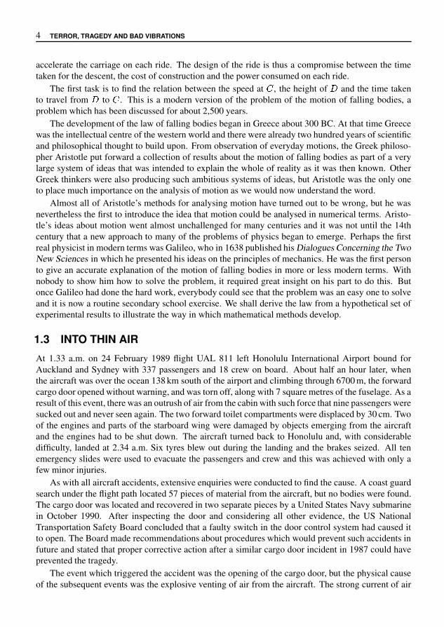
At 1.33 a.m. on 24 February 1989 flight UAL 811 left Honolulu International Airport bound forAuckland and Sydney with 337 passengers and 18 crew on board. About half an hour later, whenthe aircraft was over the ocean 138 km south of the airport and climbing through 6700 m, the forwardcargo door opened without warning, and was torn off, along with 7 square metres of the fuselage. As aresult of this event, there was an outrush of air from the cabin with such force that nine passengers weresucked out and never seen again. The two forward toilet compartments were displaced by 30 cm. Twoof the engines and parts of the starboard wing were damaged by objects emerging from the aircraftand the engines had to be shut down. The aircraft turned back to Honolulu and, with considerabledifficulty, landed at 2.34 a.m. Six tyres blew out during the landing and the brakes seized. All tenemergency slides were used to evacuate the passengers and crew and this was achieved with only afew minor injuries.
As with all aircraft accidents, extensive enquiries were conducted to find the cause. A coast guardsearch under the flight path located 57 pieces of material from the aircraft, but no bodies were found.The cargo door was located and recovered in two separate pieces by a United States Navy submarinein October 1990. After inspecting the door and considering all other evidence, the US NationalTransportation Safety Board concluded that a faulty switch in the door control system had caused itto open. The Board made recommendations about procedures which would prevent such accidents infuture and stated that proper corrective action after a similar cargo door incident in 1987 could haveprevented the tragedy.
The event which triggered the accident was the opening of the cargo door, but the physical causeof the subsequent events was the explosive venting of air from the aircraft. The strong current of air
INTO THIN AIR 5
Figure 1.3: Flight UAL811
was apparent to all on board. After the initial outrush of air, the situation in the aircraft stabilised,but passengers found it difficult to breathe. A first attempt to explain this event might be that thespeed of the aircraft through the still air outside caused the air inside to be sucked out. There areseveral reasons why this is not convincing. Firstly, the phenomenon does not occur at low altitudes.If a window is opened in a fast moving car or a low flying light aircraft, the air is not sucked out.Secondly, the same breathing difficulties are experienced on high mountains when no motion at all istaking place. It appears that the atmosphere becomes thinner in some way as height increases, andthat, as a result, it is difficult to inhale sufficient air by normal breathing. In addition, if air at normalsea level pressure is brought in contact with the thin upper level air, as occurred in the accident withflight 811, there will be a flow of air into the region where the air is thin.
The physical mechanism which is at the heart of the events described above is also involvedin a much less dramatic phenomenon and it was in this other situation that the explanation of themechanism first emerged historically.
AtmosphericPressure
Vacuum
Mercury
Figure 1.4: Barometer
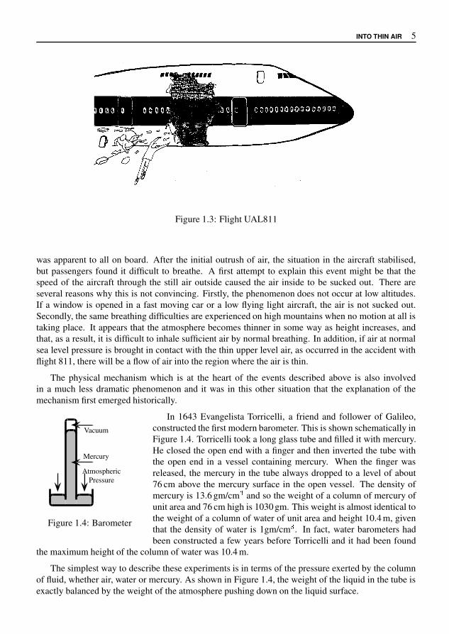
In 1643 Evangelista Torricelli, a friend and follower of Galileo,constructed the first modern barometer. This is shown schematically inFigure 1.4. Torricelli took a long glass tube and filled it with mercury.He closed the open end with a finger and then inverted the tube withthe open end in a vessel containing mercury. When the finger wasreleased, the mercury in the tube always dropped to a level of about76 cm above the mercury surface in the open vessel. The density ofmercury is 13.6 gm/cm � and so the weight of a column of mercury ofunit area and 76 cm high is 1030 gm. This weight is almost identical tothe weight of a column of water of unit area and height 10.4 m, giventhat the density of water is 1gm/cm � . In fact, water barometers hadbeen constructed a few years before Torricelli and it had been found
the maximum height of the column of water was 10.4 m.
The simplest way to describe these experiments is in terms of the pressure exerted by the columnof fluid, whether air, water or mercury. As shown in Figure 1.4, the weight of the liquid in the tube isexactly balanced by the weight of the atmosphere pushing down on the liquid surface.
6 TERROR, TRAGEDY AND BAD VIBRATIONS
Earth
Height 0 mPressure 1013 mb
Height 5000 mPressure 540 mb
Height 10 000 mPressure 264 mb
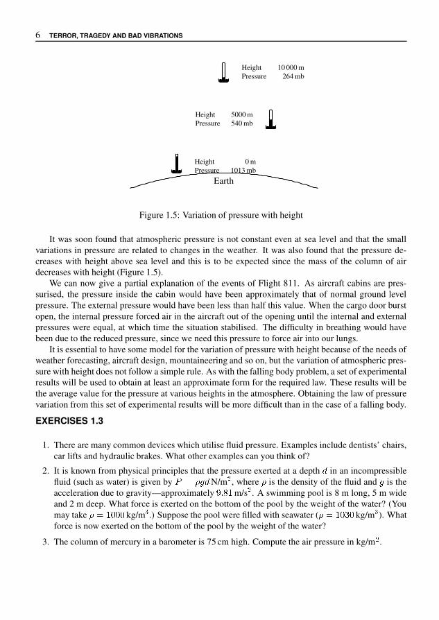
Figure 1.5: Variation of pressure with height
It was soon found that atmospheric pressure is not constant even at sea level and that the smallvariations in pressure are related to changes in the weather. It was also found that the pressure de-creases with height above sea level and this is to be expected since the mass of the column of airdecreases with height (Figure 1.5).
We can now give a partial explanation of the events of Flight 811. As aircraft cabins are pres-surised, the pressure inside the cabin would have been approximately that of normal ground levelpressure. The external pressure would have been less than half this value. When the cargo door burstopen, the internal pressure forced air in the aircraft out of the opening until the internal and externalpressures were equal, at which time the situation stabilised. The difficulty in breathing would havebeen due to the reduced pressure, since we need this pressure to force air into our lungs.
It is essential to have some model for the variation of pressure with height because of the needs ofweather forecasting, aircraft design, mountaineering and so on, but the variation of atmospheric pres-sure with height does not follow a simple rule. As with the falling body problem, a set of experimentalresults will be used to obtain at least an approximate form for the required law. These results will bethe average value for the pressure at various heights in the atmosphere. Obtaining the law of pressurevariation from this set of experimental results will be more difficult than in the case of a falling body.
EXERCISES 1.3
1. There are many common devices which utilise fluid pressure. Examples include dentists’ chairs,car lifts and hydraulic brakes. What other examples can you think of?
2. It is known from physical principles that the pressure exerted at a depth � in an incompressiblefluid (such as water) is given by � � � � � N/m , where � is the density of the fluid and � is theacceleration due to gravity—approximately � � � m/s . A swimming pool is 8 m long, 5 m wideand 2 m deep. What force is exerted on the bottom of the pool by the weight of the water? (Youmay take � � � � � � kg/m� .) Suppose the pool were filled with seawater ( � � � � � � kg/m � ). Whatforce is now exerted on the bottom of the pool by the weight of the water?
3. The column of mercury in a barometer is 75 cm high. Compute the air pressure in kg/m .

MUSIC AND THE BRIDGE 7
4. A pump is a device which occurs in many situations—pumping fuel in automobiles, pumping
Piston
LowerValve
UpperValves
Water
water from a tank or borehole or pumping gas in air con-ditioners or refrigerators. A simple type of water pump isshown in the diagram on the left. A cylinder containing apiston is lowered into a tank. The cylinder has a valve atits lower end and there are valves on the piston. When thepiston is moving down, the valve in the cylinder closes andthe valves in the piston open. When the piston moves up,the valve in the cylinder opens and the valves in the pistonclose. Based on the discussion on air pressure given in thetext, explain how such a system can be used to pump wa-ter from the tank. Explain also why the maximum height towhich water can be raised with such a pump is about 10.4 m.
1.4 MUSIC AND THE BRIDGE
Almost everyone enjoys a quiet night at home, but in the modern world there is less and less oppor-tunity for this simple pleasure. Whether it is aircraft noise, loud parties, traffic din or sporting events,there are many forms of noise pollution which cause annoyance or disruption. New forms of noisepollution are continually arising and some of these are quite unexpected.
Sydney contains a large number of bridges, the best known of these being the Sydney HarbourBridge. The newest bridge is the A$170m Anzac Bridge, originally known as the Glebe Island Bridge(Figure 1.6). The main span of this concrete bridge is 345 m long and 32.2 m wide. The deck issupported by two planes of stay cables attached to two 120 m high reinforced concrete towers. Itis the cables which created an unexpected problem. As originally designed, they were enclosed inpolyurethane coverings. When the wind was at a certain speed from the south-east, the cables beganto vibrate and bang against the coverings. The resulting noise could be heard several kilometres awayfrom the bridge, much to the annoyance of local residents. Engineers working on the bridge had tofind a way to damp the vibrations and thereby reduce or eliminate the noise.
As with the previous two problems, this problem is a modern version of one that has been inexistence for many centuries. The form in which it principally arose in the past was in relation to thesounds made by stringed instruments such as violins and guitars. In these instruments a metal stringis stretched between two supports and when the string is displaced by plucking or rubbing it begins tovibrate and emit a musical note.
The frequency of the note is the same as the frequency of the vibrations of the string and so theproblem becomes one of relating the frequency of vibration to the properties of the string. In the caseof the bridge, the aim is to prevent the vibrations or else to damp them out as quickly as possible whenthey begin.
The analysis of the vibrations is a complex problem which can be approached in stages, beginningwith the simplest possible type of model. Any vibrating system has a natural frequency at which itwill vibrate if set in motion. If a force is applied to the system which tries to make it vibrate at thisfrequency, then the system will vibrate strongly and in some systems catastrophic results can followif the vibrations are not damped out. An example of this is one of the most famous bridge collapses inhistory. This occurred on 7 November 1940, when the Tacoma Narrows Bridge in the United Stateshad only been open for a few months. A moderately strong wind started the bridge vibrating withits natural frequency. The results were spectacular. News movies show the entire bridge oscillatingwildly in a wave-like motion before it was finally wrenched apart.

8 TERROR, TRAGEDY AND BAD VIBRATIONS
Figure 1.6: The Anzac Bridge
With the Anzac Bridge, the vibrations caused annoyance rather than catastrophe, but the problemneeded to be dealt with. The first step is to find, at least approximately, the natural frequency of thevibration of the cables supporting the bridge. Once this frequency is known, then measures can betaken to damp the vibrations.
EXERCISES 1.4
1. What factors do you think are significant in determining the frequency of vibration of a string orcable stretched between two supports? Explain how these factors allow a stringed instrument tobe tuned.
2. Musical instruments such as guitars, violins, cellos and double basses rely on vibrating strings toproduce sound. Explain why a double bass sounds so different to a violin.
1.5 DISCUSSIONThe three problems we have outlined are very different, but they have some features in common. Ineach of them there is a complex system which can be described in terms of a collection of properties.The properties may describe the system itself or its mode of operation. Some of these propertiescan be assigned numerical values while others cannot. For example, in the three problems we havedescribed, the time taken for the car to fall from
�to
�, the atmospheric pressure and the frequency at
which the cables vibrate are all numerical properties. On the other hand, the amount of terror causedby the ride, the difficulty experienced by passengers in breathing or the beauty of the bridge do nothave exact numerical values.
In the mathematical analysis of problems, we will only consider the numerical properties of ob-jects or systems. It often happens that we may wish to calculate some numerical property of a systemfrom a knowledge of other numerical properties of the system. In almost all such cases, calculatinga numerical value will involve the concept of a function. We will become quite precise about thisconcept in the next chapter, but for the moment we shall consider a few special cases.

RULES OF CALCULATION 9
In the Tower of Terror, there are a number of possibilities. We may wish to know the height � ofthe car at any time � , or the velocity � at any time � , or the velocity � at a given height � . Suppose weconsider the variation of height with respect to time. We let � be the height above the baseline, whichis taken to be the level of
�in Figure 1.2. This height changes with time and for each value of � , there
is a unique value of � . This is because at a given time the car can only be at one particular height. Or,to put it another way, the car cannot be in two different places at the same time. On the other hand,the car may be at the same height at different times; two different values of � may correspond to thesame value of � . The quantities � and � are often referred to as variables. Notice also that the twoquantities � and � play different roles. It is the value of � which is given in advance and the value of
� which is then calculated. We often call � the independent variable, since we are free to choose itsvalue independently, while � is called the dependent variable, since its value depends on our choiceof � .
In the second problem, we have a similar situation. We wish to find a rule which enables us tofind the pressure � at a given height � . Here we are free to choose � (as long as it is between � andthe height of the atmosphere), while � depends on the choice of � , so that � is the dependent variableand � is the independent variable.
Finally, in the case of the Anzac Bridge, we can represent one of the cables schematically asshown in Figure 1.7. In the figure, the cable is fixed under tension between two points
�and
�. If
it is displaced from its equilibrium position, it will vibrate. To find the frequency of the vibrationwe need a rule which relates the displacement of the center of the cable to the time � . Here theindependent variable is � , the dependent variable is and we want a computational rule which enablesus to calculate if we are given � .
� �
Figure 1.7: A vibrating cable
In a given problem, there is often a natural way of choosing which variable is to be the independentone and which is to be the dependent one, but this may depend on the way in which the problem isposed. For example, in the case of air pressure, we can use a device known as an altimeter to measureheight above the earth’s surface by observing the air pressure. In this case, pressure would be theindependent variable, while height is the dependent variable.
1.6 RULES OF CALCULATIONEach of the above problems suggests that to get the required numerical information, we need a rule ofcalculation which relates two variables. There are many ways of arriving at such rules—we may useour knowledge of physical processes to deduce a mathematical rule of calculation or we may simplyobserve events and come to trial and error deductions about the nature of the rule.
Let us try to distil the essential features of rules of calculation which can be deduced from thethree examples we have presented:
The independent variable may be restricted to a certain range of numbers. For instance, in the
10 TERROR, TRAGEDY AND BAD VIBRATIONS
case of the Tower of Terror we might not be interested in considering values of time � before themotion of the car begins or after it ends. In the case of atmospheric pressure, the height mustnot be less than zero, nor should it extend to regions where there is no longer any atmosphere.This range of allowed values of the independent variable will be called the domain of the rule.
� There has to be a procedure which enables us to calculate a value of the dependent variable foreach allowable value of the independent variable.
� To each value of the independent variable in the domain, we get one and only one value of thedependent variable.
In the next chapter, we shall formalise these ideas into the concept of a function, one of the mostimportant ideas in mathematics.
EXERCISES 1.6
1. The pressure on the hull of a submarine at a depth � is � . Explain how we can regard either of thevariables � and � as the independent variable and the other as the dependent variable. Suggest areasonable domain when � is the independent variable.
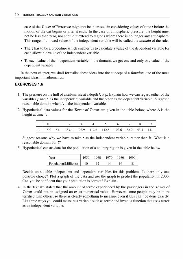
2. Hypothetical data values for the Tower of Terror are given in the table below, where � is theheight at time � .
�0 1 2 3 4 5 6 7 8 9
�15.0 54.1 83.4 102.9 112.6 112.5 102.6 82.9 53.4 14.1
Suggest reasons why we have to take � as the independent variable, rather than � . What is areasonable domain for � ?
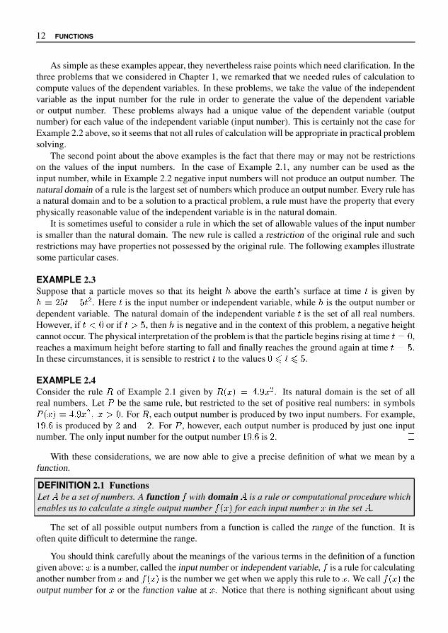
3. Hypothetical census data for the population of a country region is given in the table below.
Year 1950 1960 1970 1980 1990
Population(Millions) 10 12 14 16 18
Decide on suitable independent and dependent variables for this problem. Is there only onepossible choice? Plot a graph of the data and use the graph to predict the population in 2000.Can you be confident that your prediction is correct? Explain.
4. In the text we stated that the amount of terror experienced by the passengers in the Tower ofTerror could not be assigned an exact numerical value. However, some people may be moreterrified than others, so there is clearly something to measure even if this can’t be done exactly.List three ways you could measure a variable such as terror and invent a function that uses terroras an independent variable.

CHAPTER 2FUNCTIONS
In this chapter we will give a detailed discussion of the concept of a function, which we brieflyintroduced in Chapter 1. As we have indicated, a function is a rule or calculating procedure fordetermining numerical values. However, the nature of the real world may impose restrictions on thetype of rule allowed.
2.1 RULES OF CALCULATION
In the problems we shall consider,we require rules of calculation which operate on numbers to produceother numbers. The number on which such a rule operates is called the input number , while thenumber produced by applying the rule is called the output number . Let us denote the input numberby � , the rule by letters such as � � � � and the corresponding output numbers by � � � � � � � � � � .Thus a rule � operates on the input number � to produce the output number � � � � . We can illustratethis idea schematically in the diagram below.
�� � � � �
Here we think of a function as a machine into which we enter the input number � . The machinethen produces the output � � � � according to the rule given by � . A concrete example of such amachine is the common calculator.
EXAMPLE 2.1Let � be the rule which instructs us to square the input number and then multiply the result by � � .In symbols we write � � � � � � � � � . Thus, if the input number is � ! , then its square is � " ! andmultiplying this by � � gives the output number as � $ & ( � .
EXAMPLE 2.2Let � be the rule which instructs us to find a number whose square is the input number. In symbols,
� � � � is given by � � � � � � � � � . Thus if the input number is � , there are two possible values for theoutput number � � � � , namely , . and . . /
12 FUNCTIONS
As simple as these examples appear, they nevertheless raise points which need clarification. In thethree problems that we considered in Chapter 1, we remarked that we needed rules of calculation tocompute values of the dependent variables. In these problems, we take the value of the independentvariable as the input number for the rule in order to generate the value of the dependent variableor output number. These problems always had a unique value of the dependent variable (outputnumber) for each value of the independent variable (input number). This is certainly not the case forExample 2.2 above, so it seems that not all rules of calculation will be appropriate in practical problemsolving.
The second point about the above examples is the fact that there may or may not be restrictionson the values of the input numbers. In the case of Example 2.1, any number can be used as theinput number, while in Example 2.2 negative input numbers will not produce an output number. Thenatural domain of a rule is the largest set of numbers which produce an output number. Every rule hasa natural domain and to be a solution to a practical problem, a rule must have the property that everyphysically reasonable value of the independent variable is in the natural domain.
It is sometimes useful to consider a rule in which the set of allowable values of the input numberis smaller than the natural domain. The new rule is called a restriction of the original rule and suchrestrictions may have properties not possessed by the original rule. The following examples illustratesome particular cases.
EXAMPLE 2.3Suppose that a particle moves so that its height � above the earth’s surface at time � is given by
� � � � � � � � . Here � is the input number or independent variable, while � is the output number ordependent variable. The natural domain of the independent variable � is the set of all real numbers.However, if � � � or if � � � , then � is negative and in the context of this problem, a negative heightcannot occur. The physical interpretation of the problem is that the particle begins rising at time � � � ,reaches a maximum height before starting to fall and finally reaches the ground again at time � � � .In these circumstances, it is sensible to restrict � to the values � � � � � .
EXAMPLE 2.4Consider the rule � of Example 2.1 given by � � � � # % & � . Its natural domain is the set of allreal numbers. Let ( be the same rule, but restricted to the set of positive real numbers: in symbols
( � � � # % & � + � � � . For � , each output number is produced by two input numbers. For example,- & % 0 is produced by � and � � . For ( , however, each output number is produced by just one inputnumber. The only input number for the output number - & % 0 is � . 2
With these considerations, we are now able to give a precise definition of what we mean by afunction.
DEFINITION 2.1 FunctionsLet
3be a set of numbers. A function 4 with domain
3is a rule or computational procedure which
enables us to calculate a single output number 4 � � for each input number � in the set3
.
The set of all possible output numbers from a function is called the range of the function. It isoften quite difficult to determine the range.
You should think carefully about the meanings of the various terms in the definition of a functiongiven above: � is a number, called the input number or independent variable, 4 is a rule for calculatinganother number from � and 4 � � is the number we get when we apply this rule to � . We call 4 � � theoutput number for � or the function value at � . Notice that there is nothing significant about using

RULES OF CALCULATION 13
the letter � to denote a function or the letter � for the independent variable. A function is some ruleof calculation and as long as we understand what the rule is, it doesn’t matter what letter we use torefer to the function. We can even specify a function without using such letters at all. We simplyshow the correspondence between the input number and the output number. Thus the function � ofExample 2.1 defined by � � � � � � � � � may be written as � � � � � � � � . We read this as � goes to (ormaps to) � � � � � . Common letters to denote functions are � � � and � . Various Greek letters such as� � � or
�are also used. The independent variable is a number such as � or � � � " $ , and it is irrelevant
whether we denote it by % , � or any other letter.
EXAMPLE 2.5We define a function � by the rule
� � % � � % + " % � � % / 1 �We also define a function
�by the rule
� � � � � � + " � � � � / 1 �You should convince yourself that � and
�define the same function. 4
In order to completely specify a function, it is necessary to give both the domain and the rule forcalculating function values from numbers in the domain. In practice, it is common to give only therule of calculation without specifying the domain. In this case it is assumed that the domain is the setof all numbers which produce an output number when the rule of calculation is applied. This is calledthe natural domain of the function.
EXAMPLE 2.6We define a function � by the rule
� � % � % �
where % can be any real number. We can compute � � % � for all % 6 7 , so that the natural domain of thefunction is the set of all numbers % for which either 8 9 ; % ; 7 or 7 ; % ; 9 . Its range is the sameset of numbers.
EXAMPLE 2.7Let � � � � � � � + � + . Find � � " � , � � 8 � � and � � � � � .Solution
� � " � � � " � � + " + � �
� � 8 � � � � 8 � � � + � 8 � � + � � � 8 � +
� � � � � � � � � � � + � � � � + H � � + � � +

14 FUNCTIONS
EXERCISES 2.1
In Exercises 1–7, find the numerical value of the function at the given values of � .
1. � � � � � � � � � � � � 2. � � � � � �� � � � � � �3. � � � � � if � " $ if � % � � $ � � � �4. � � , � $� , � � , � 5. 0 � � � $ � $� $ � � � � � � �6.
6 � 7 � $ � 9 � 7 < 9 � � � 7. � � � � � > $$ ? � � � � � � B � �In Exercises 8–12, calculate � � � � � � � $ F � � and � � � � $ � B
8. � � � � � � � � 9. � � � � $�10. � � � � � � $� � � $ 11. � � � � � � $12. � � � � � � � � $ if � " �� � > ? if � % �13. In Figure 1.2 on page 3, let I be the velocity of the carriage at time , and let 0 be the vertical
height aboveJ
at time , . The total energy K at time , is defined to be
K N� O I � � O � 0 �where � R B S $ m/s � is a constant and O is the mass of the carriage. There is a physical law,known as the principle of conservation of energy, which states that K is a constant.
(a) If the velocity atJ
is 162 km/hr, what is the velocity atJ
in m/s?
(b) Suppose the vertical distance ofT
fromJ
is 14 m. Use the principle of conservation ofenergy to calculate the vertical distance
T U.
14. Do you think that it is meaningful to consider physical quantities for which no method of mea-surement is known or given?
15. The population V (in millions) of a city is given by a function � whose input number is the timeelapsed since the city was founded in 1876. We have V � � , � . Explain the meaning of thestatement V � $ ? � � � .
16. Functions � , � and 0 are defined by the rules
� � � � � � � � � � � � � > � � �� � � $ � 0 � � � � � > � �� � $ BExplain why � � , but � ^ 0 � � ^ 0 .
17. Express the distance between the origin and an arbitrary point � � _ � 7 _ � on the line � � � 7 $ interms of � _ .
INTERVALS ON THE REAL LINE 15
18. Let � � � � � � � � . When does � � � � equal � � and when does it equal � � ?
19. Express the following statements in mathematical terms by identifying a function and its rule ofcalculation.
(a) The number of motor vehicles in a city is proportional to the population.
(b) The kinetic energy of a particle is proportional to the square of its velocity.
(c) The surface area of a sphere is proportional to the square of its radius.
(d) The gravitational force between two bodies is proportional to the product of their masses�and � and inversely proportional to the square of the distance � between them.
20. Challenge problem: The following function�
is defined for all positive integers � and knownas McCarthy’s 91 function.
� � � � � � � � � if � � � � � �� � � � � ! � � � � if � % � � � &Show that
� � � � ( � for all positive integers � % � � � .
2.2 INTERVALS ON THE REAL LINEThe domain of a function is often an interval or set of intervals and it is useful to have a notation fordescribing intervals.) The closed interval * + � . 0 is the set of numbers � satisfying + % � % . .) The open interval � + � . � is the set of numbers � satisfying + 4 � 4 . .) � + � . 0 denotes the set of numbers � satisfying + 4 � % . .) * + � . � denotes the set of numbers � satisfying + % � 4 . .
We also need to consider so-called infinite intervals.) The notation * + � 6 � denotes the set of all numbers � 9 + , while � 6 � + 0 denotes the set of allnumbers � % + .) The notation � + � 6 � denotes the set of all numbers � � + , while � 6 � + � denotes the set of allnumbers � 4 + .) We can also use � 6 � 6 � to denote the set of all real numbers, but this is usually denoted bythe special symbol ? .
A little set notation is also useful. Let @ be an interval on the real line. If � is a number in @ , thenwe write � A @ . This is read as � is in @ , or � is an element of @ .
Next, let @ C and @ D be any two intervals on the real line. Then @ C E @ D denotes the set of all numbers� for which � A @ C or � A @ D . Note that the mathematical use of the word “or” is not exclusive. Italso allows � to be an element of both @ C and @ D . We call @ C E @ D the union of @ C and @ D .
We use @ C I @ D to denote the set of all numbers � for � A @ C and � A @ D . We call @ C I @ D theintersection of @ C and @ D . It may happen that @ C and @ D have no elements in common, in which casethe intersection of @ C and @ D is said to be empty. We write @ C I @ D J in this case.
Finally, we use the notation @ C K @ D to denote the elements of @ C which are not also in @ D .

16 FUNCTIONS
EXAMPLE 2.8For the function � � � � � � � � of Example 2.1, the domain is � � � � � � , while the range is � � � � � .For the function � � � � � � � � , � ! � of Example 2.4, both the domain and range are � � � � � .
EXAMPLE 2.9Let # $ � % � � � and # � � * � , � . Then # $ . # � � % � , � , # $ / # � � * � � � and # $ 1 # � � % � * 4 .EXAMPLE 2.10The natural domain of the function
5 � � � %�
is � � � � � � . � � � � � .
EXERCISES 2.2
In Exercises 1–6, find the domain and range of the function. Express your answer in the intervalnotation introduced in this section.
1. 5 � � � 9 � 9 2. 5 � � � %� � %
3. 5 � � � = % � @ � 4. 5 � � � �� � � * � � � C % �
5. E � � � � � � � H � J % 6. K � � � = � C * � � O �7. Express the area of a circle as a function of its circumference, that is, find a function 5 for which
the output number 5 � P � is the area whenever the input numberP
is the circumference. What isthe domain of the function?
8. Express the area of an equilateral triangle as a function of the length of one of its sides.
Rewrite the expressions in Exercises 9–14 as inequalities.
9. � Q � , � T 4 10. � Q � % � � � 11. � Q � % � @ �12. � Q � % � � 4 . � % � � � � 13. � Q � � % � � � / � @ � W � 14. � Q � � � � � �
Rewrite the following expressions in interval notation.
15. @ H � J * 16. � ! Y 17. � Q [18. � O % @ 19. 9 � C * 9 J � 20. 9 � 9 O @21. � % J � J * and � ! ,

GRAPHS OF FUNCTIONS 17
2.3 GRAPHS OF FUNCTIONSIf � is a function with domain
�, then its graph is the set of all points of the form � � � � � � � � , where �
is any number in�
(written � � �). It is often difficult to sketch graphs, but one method is simply to
plot points until we can get an idea of the nature of the graph and then join these points, as we havedone in Example 2.11 below. The procedure for any other example is no different—it may just takelonger to compute the function values. In many cases there are shorter and more elegant ways to plotthe graph, but we shall not investigate these methods in any detail.
EXAMPLE 2.11Let the function � be defined by the rule � � � � � � � . We tabulate values of � � � � for various valuesof � :
� � � � � � � � � 0 1 2 3 4
� � � � 16 9 4 1 0 1 4 9 16
If these points are now plotted on a diagram the general trend is immediately evident and we canjoin the points with a smooth curve. This is shown schematically in the diagram below, which wehave plotted using the software package Mathematica.
-4 -2 2 4
5
10
15
Figure 2.1: The graph of � � � � � � �
!Why do we draw graphs? One of the main reasons is as an aid to understanding. It is often easier
to interpret information if it is presented visually, rather than as a formula or in tabular form. With theadvent of computer software such as Mathematica and Maple, the need to plot graphs by hand is notas great as it used to be. Computers plot graphs in a similar way to the above example—they calculatemany function values and then join neighbouring points with straight lines. Because the plotted pointsare so close together, the straight line segments joining them are very short, and the overall impressionwe get from looking at the graph is that a curve has been drawn.
2.3.1 Plotting graphs with Mathematica
The instruction for plotting graphs with Mathematica is Plot. The essential things that Mathematicaneeds to know are the function to be plotted, the independent variable and the range of values for the

18 FUNCTIONS
independent variable. There are numerous optional extras such as colour, axis labels, frames and soon. In this book we will explain how to use Mathematica to perform certain tasks, but we will assumethat you are familiar with the basics of Mathematica, or have access to supplementary material.1
EXAMPLE 2.12To plot a graph of the function given by � � � � � � , we use the instruction
Plot[xˆ2,{x,-4,4}]
This will produce the following graph:
-4 -2 2 4
2.5
5
7.5
10
12.5
15
Figure 2.2: A basic Mathematica plot
This graph does not look as nice as the one in Example 2.1. The vertical axis is too crowded, thecurve is rather squashed and there is no colour. To improve the appearance, we can add a few moreoptions. To plot the graph in Example 2.1 (without the dot points), we used the instruction
Plot[xˆ2,{x,-4,4},PlotStyle->{RGBColor[1,0,0]},Ticks->{{-4,-2,0,2,4},{5,10,15,20}},AspectRatio->1]
Here the Ticks option selects the numbers that we wish to see on the axes, while AspectRatioalters the ratio of the scale on the two axes. Notice that Mathematica may sometimes choose tooverride our instructions. In this case it has not put a tick for � � � . The numbers in RGBColorgives the ratios of red, green and blue. In this case the graph is 100% red.2 �
EXERCISES 2.3
1. Use the Mathematica instruction given in the text to plot the graph of � � � � � � . Experimentwith different colours and aspect ratios to see how the appearance of the graph changes.
1For example, Introduction to Mathematica by G. J. McLelland, University of Technology, Sydney, 1996.2The current edition of this book has not been printed in colour. However, you can get colour graphs on a computer by
following the given commands.

GRAPHS OF FUNCTIONS 19
2. Plotting a graph over a part of its domain can lead to deceptive conclusions about the nature ofthe graph in its entire domain. By selecting a suitable interval, obtain the following plots for
� � � � � � and � � � � � . In each case, the dotted plot is the graph of . What would you haveconcluded had you plotted only one of these graphs?
3. Here is a table of values which could apply to the Tower of Terror.
� 0 1 2 3 4 5 6 7 8 9
� 15.0 54.1 83.4 102.9 112.6 112.5 102.6 82.9 53.4 14.1
(a) Use the command
a= � � 0,15 � , � 1,54.1 � , � 2,83.4 � , � 3,102.9 � , � 4,112.6 � ,� 5,112.5 � , � 6,102.6 � , � 7,82.9 � , � 8,53.4 � , � 9,14.1 � �
to enter this table as a list in a Mathematica notebook.
(b) Use the Mathematica command ListPlot in the form
g0=ListPlot[a,PlotStyle->PointSize[0.02]]
to plot these points on a graph. Notice that these points lie on what appears to be a smooth curve.Print a copy of the graph, join the points by hand with a smooth curve and use this curve toestimate the height after 2.5 s.
(c) Rather than estimate the curve by joining the points by hand, we can use the Mathematicacommand Fit. This command fits a curve of the user’s choice (straight line, quadraticpolynomial and so on) to a list of data points. There are numerous options and you shouldconsult the Mathematica help files for a full explanation of this command. The command
f1=Fit[a, � 1,x � ,x]
will give a formula for the best straight line fitting the given points. Similarly, the com-mands
f2=Fit[a, � 1,x,x � 2 � ,x]f3=Fit[a, � 1,x,x � 2,x � 3 � ,x]
will give a formula for the best quadratic and best cubic polynomial respectively fitting the givenpoints. Fit a quadratic polynomial to the points in the above table, that is, find f2. Use thisformula to calculate the height at each of the times given in the table. How good is the agreement?What conclusions can you draw about the data? Determine the height after 2.5 seconds. Doesthis agree with your answer in part (b)?

20 FUNCTIONS
(d) You can plot the formula f2 with the instruction
g2=Plot[f2, � x,0,10 � ]
Do this, and then display the graph g2 and the plotted points g0 simultaneously by usingthe instruction
Show[g0,g2]
4. Here is a table giving the atmospheric pressure at different heights:
� 0 1000 2000 3000 4000 5000 6000 7000 8000 9000 10 000
� 1013 899 795 701 616 540 472 411 356 307 264
(a) Enter this table as a list in a Mathematica notebook
(b) Plot these points on a graph. Notice that these points lie on what appears to be a smoothcurve. Print a copy of the graph, join the points with a smooth curve and use this curve toestimate the pressure at a height of 4500 metres.
(c) Fit a straight line, a quadratic polynomial and a cubic polynomial to the set of points inthe table above. In each case, use the formula to calculate the pressure at the heightsgiven in the table and compare the results with the tabulated values. Which curve gives thebest approximation to the table values? Compute the pressure at a height of 4500 m andcompare it with your result in part (b).
(d) On the same set of axes, plot the graphs of the functions obtained in part (c).
5. A airplane flying from Tullamarine Airport in Melbourne to Kingsford-Smith in Sydney has tocircle Kingsford-Smith several times before landing. Plot a graph of the distance of the airplanefrom Melbourne against time from the moment of takeoff to the moment of landing.
6. A rectangle of height � is inscribed in a circle of radius � . Find an expression
���
for the area of the rectangle. Plot a graph of this area as a function of �and decide from your graph at what value of � the area of the rectangleis a maximum.
2.4 EXAMPLES OF FUNCTIONSIn this section, we consider various examples of functions. Looking at different examples is a usefullearning method in mathematics and one which you should try to cultivate. Very often, mathematicalconcepts possess subtleties which are not immediately apparent. Studying and doing many examplesexposes you to many different aspects of a concept and should help your learning. Before giving theseexamples, there is one matter which needs to be clarified, and that is the one posed by the followingquestion:
What do we mean when we say that a given function � , say, is known or well-defined?
In this book, we emphasise the use of functions to compute numerical data relating to problems inthe real world. This implies that when we use a function to calculate the value of the dependent
EXAMPLES OF FUNCTIONS 21
variable in a practical problem, the answers we get should agree with the experimental data. As faras such data is concerned, the only values which are measured in the real world are decimal numbersto a certain accuracy. Since more sophisticated methods of measurement may increase accuracy, therule that defines a function should be able to produce output numbers in decimal form with arbitraryaccuracy. If the rule does not allow us to do this, then we cannot really say that the function is known.Accordingly, one answer to the question posed above is:
We say that the function � is known or, more technically, is well-defined, if we are able tocompute � � � � in decimal form to an arbitrary degree of accuracy, for any � in the domainof � .
For example, the rule � of Example 2.1 given by � � � � � � � � � enables us to compute � � � � to anynumber of decimal places that we choose. Computing an output number such as � � � � � � � � � � � � � �to any degree of accuracy can be done, although it may take some time.3 Thus � is a well-definedfunction.
Now let us turn to some examples. In describing any function, we must insist on three things:
1. The domain of the function must be known. (But see the remark on page 13 about naturaldomains.)
2. There must be a rule which produces one (and only one) output number for each input numberin the domain.
3. The rule must be in a form which enables us to compute the output number to any specifieddegree of accuracy.
One simple way of defining functions is by arithmetic operations—addition, subtraction, multipli-cation and division, and the simplest functions of this type are polynomials. These consist of sums ofthe form
� � � � � # $ � $ % # $ ' ( � $ ' ( % * * * % # ( � % # , -
where # , - # ( - � � � - # $ are constants for a given � .
EXAMPLE 2.13A function � defined by the rule
� � � � � � 1 2 � � % � % �
is a polynomial function. We can compute its value for any input number, for example
� � � � � � � � � � 1 2 ; � � � � % � � � % �
� � � � � � 2 � � � � % � � � % �
� 2 � � � � � �
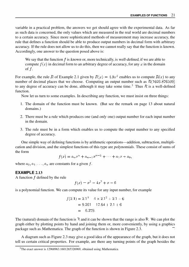
The (natural) domain of the function is B and it can be shown that the range is also B . We can plot thegraph either by plotting points by hand and joining them or, more conveniently, by using a graphicspackage such as Mathematica. The graph of the function is shown in Figure 2.3. C
A diagram such as Figure 2.3 may give a good idea of the appearance of the graph, but it does nottell us certain critical properties. For example, are there any turning points of the graph besides the
3The exact answer is 12968963.1601265326969, obtained using Mathematica.
22 FUNCTIONS
� � �� �� ��
� �
�
Figure 2.3: The graph of � � � � � � � � � � � � � �ones shown? In many cases of interest, the domain of a function is an infinite interval, in which casewe can only plot part of its graph. We cannot then be sure about features, such as turning points, thatmay occur in the region we have not plotted. In Figure 2.3 all the turning points of the graph havebeen plotted, but we would need to do some further mathematical analysis to show this.
In the above example, we have specified the rule for calculating function values by giving a for-mula which applies at all points of the domain. However, the rule for calculating function values maybe given by a different formula at different points of the domain, as the following example shows.
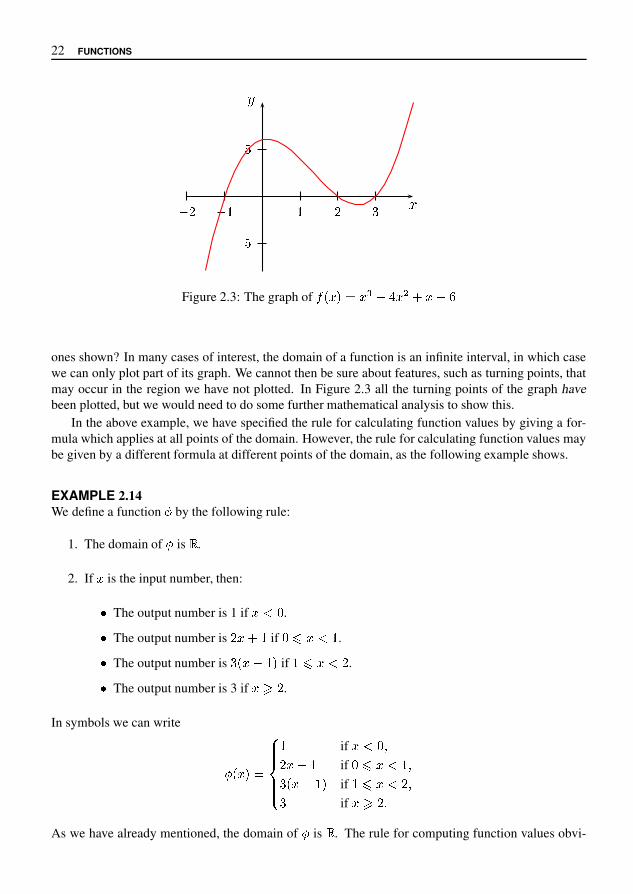
EXAMPLE 2.14We define a function
�by the following rule:
1. The domain of�
is .
2. If � is the input number, then:! The output number is 1 if � # $ .! The output number is � � � � if $ ( � # � .! The output number is � � � � � � if � ( � # � .! The output number is 3 if � / � .
In symbols we can write
� � � � � 2 33343335
� if � # $ 7� � � � if $ ( � # � 7� � � � � � if � ( � # � 7� if � / � ;As we have already mentioned, the domain of
�is . The rule for computing function values obvi-
EXAMPLES OF FUNCTIONS 23
ously produces numerical values of any accuracy:� � � � � � � � � � � � �
� � � � � � � � � �� � � � � � �The graph of the function is shown in Figure 2.4. From the graph we see that the range is � � � � . Noticethe small circle centred at the point � � � � . Here we are using the common convention that this circleindicates that the point at its centre—in this case � � � � —is excluded from the graph. We have alsocentered a solid disk at the point � � � � to indicate that this point is included in the graph.
� � � "� �� �
�
�
�
#
$
Figure 2.4: The graph of % � � � (
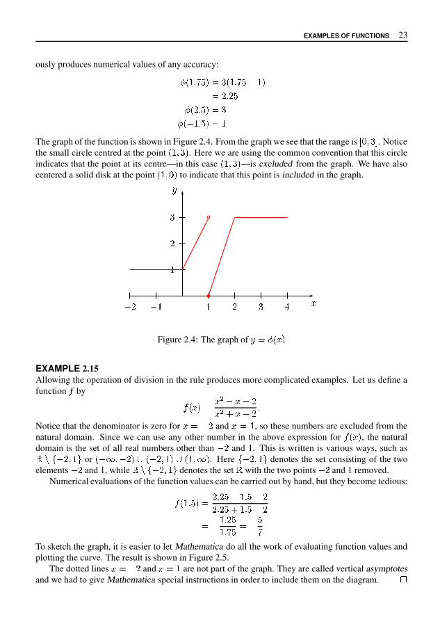
EXAMPLE 2.15Allowing the operation of division in the rule produces more complicated examples. Let us define afunction * by
* � ( � ( - � ( � �( - 1 ( � � �
Notice that the denominator is zero for ( � � � and ( � � , so these numbers are excluded from thenatural domain. Since we can use any other number in the above expression for * � ( , the naturaldomain is the set of all real numbers other than � � and � . This is written is various ways, such as
3 4 5 � � � � 7 or � � 9 � � � ; � � � � � ; � � � 9 . Here 5 � � � � 7 denotes the set consisting of the twoelements � � and 1, while 3 4 5 � � � � 7 denotes the set 3 with the two points � � and 1 removed.
Numerical evaluations of the function values can be carried out by hand, but they become tedious:
* � � � � � � � � � � � �� � � 1 � � � �
� � � � � � � � � �
�To sketch the graph, it is easier to let Mathematica do all the work of evaluating function values andplotting the curve. The result is shown in Figure 2.5.
The dotted lines ( � � � and ( � � are not part of the graph. They are called vertical asymptotesand we had to give Mathematica special instructions in order to include them on the diagram. B

24 FUNCTIONS
-4 -3 -2 -1 1 2 3
-20
-10
10
20
30
Figure 2.5: A Mathematica plot of the graph of � � � � � � � � �� � � � �
Functions defined by algebraic formulas arise in some simple applications, but in most applica-tions the functions we obtain as solutions have to be defined in other ways. We give an example ofsuch a function, whose rule of evaluation may seem strange, artificially contrived and of no practicaluse. In fact the rule is very useful in applications and a large part of our later work will be to find outwhy such rules are needed in practical problems and how we can obtain them. It would be very easy tosolve problems if the only functions we ever needed were nice simple ones. Unfortunately (or perhapsfortunately, depending on your point of view), describing phenomena in the real world is usually adifficult procedure and if we are to make any progress we need some non-trivial mathematics.
EXAMPLE 2.16We are going to define a function � by a rule which is, at first sight, unusual. If you have not seenthis rule before, you probably will have no idea of what the function is used for or where the rulecomes from. The purpose of this example is to show that no matter how complex or unusual a rulemay seem, if it is properly specified we should be able to follow it and produce an output number. Atthis point we are not going to explain what the function � is used for, but only how to calculate itsvalue for any input number. We are asking you to go through the same sort of unthinking process thata computer uses in calculations—just follow the rules. The why of this example will be clarified inChapter 6. Here is the process:
1. Let the input number � be any positive real number.
2. Select a desired accuracy of calculation � , that is, we want the calculation to give an outputnumber with an accuracy of � � .
3. Calculate each of the numbers
� � � ��
� ��
� �� �
�� !
" �� $ $ $ �
where for any % ' � , we define % � % + � % � � � + � % � � � + 3 3 3 + � + � + � . Continue until
one of the numbers is less than � . Suppose this number is� 7
8 �.
4. Then the output number for � can be calculated with an error of less than � from the expression
� 7 � � � � � � ��
� ��
� �� �
� 3 3 3 � � � � � 7 B C� 7 B C
� 8 � � � ��
EXAMPLES OF FUNCTIONS 25
that is, � � � � � � � � � � � � � � � .
As an illustration, take � � � � � and � ! � ! ! � . Then we find
� � � � � � %& ( � � � � & � � +
, ( � ! � � / & � � 23 (
�� ! � & � ! 5� 6
� (�� ! � ! / , , � 7
/ (�� ! � ! � � 8 � 9
: (�� ! � ! ! , 3 � <
8 (�� ! � ! ! ! / =
where we have worked to 4 decimal places. The notation�� is used to indicate that the number on the
right hand side is, to the stated number of decimal places, equal to the number on the left hand side.Following our rule, we get
� � � � � �� � � � � � � � � � & � � ! � � / & � � ! � & � ! 5 � ! � ! / , , � ! � ! � � 8 � � ! ! , 3� ! � & & & �
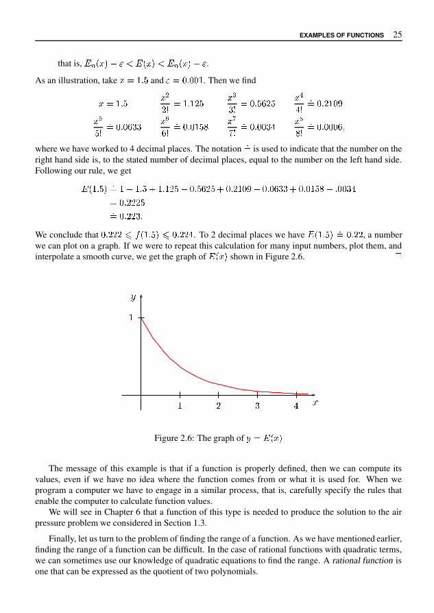
�� ! � & & , �We conclude that ! � & & & B C � � � � B ! � & & 3 . To 2 decimal places we have � � � � � �� ! � & & , a numberwe can plot on a graph. If we were to repeat this calculation for many input numbers, plot them, andinterpolate a smooth curve, we get the graph of � � � shown in Figure 2.6. H
� & , 3
�
I
J
Figure 2.6: The graph of K � � � �
The message of this example is that if a function is properly defined, then we can compute itsvalues, even if we have no idea where the function comes from or what it is used for. When weprogram a computer we have to engage in a similar process, that is, carefully specify the rules thatenable the computer to calculate function values.
We will see in Chapter 6 that a function of this type is needed to produce the solution to the airpressure problem we considered in Section 1.3.
Finally, let us turn to the problem of finding the range of a function. As we have mentioned earlier,finding the range of a function can be difficult. In the case of rational functions with quadratic terms,we can sometimes use our knowledge of quadratic equations to find the range. A rational function isone that can be expressed as the quotient of two polynomials.

26 FUNCTIONS
EXAMPLE 2.17Find the range and natural domain of the function
� � � � �� � �
It is easy to see that the natural domain is the set of all real numbers � for which � � � � . To find therange, we put
� �� �
and rearrange the equation to get � � � � � � � . This is a quadratic equation in � and we need tofind the values of � for which this equation can be solved to give real values of � . The discriminant is
� � � " � and this is well-defined for all � . Hence the range of � is $ .
EXERCISES 2.4
In Exercises 1–6, find the natural domain and range of the function.
1. � � � � � � & 2. � � � � � �� �
3. ( � * � . * � � 4. � � � � � � &
5. ( � � � � �� 6. � � � � � 4 � �
7. Let � be the function defined in Example 2.16. In this example, we found � � � � 6 � � � � � & �� � � � � . Evaluate � � � � , � � � � 6 � , � � � � and � � � � with an error of less than 0.001. Plot these valueson a graph, together with the value of � � � � 6 � . Hence verify that the graph of � is consistent withthe one given in Figure 2.6.
8. Consider the equation� � � � ( > )
For every value of � , we can find two possible values of � , namely � ? � � � and � � ? � � � . Thus, each of the above equations defines a function of � according to
� A � � � . � � � and
� � � � � . � � � �We say that � A and � are functions implicitly defined by the equation ( > ). We can also solvethe equation ( > ) for � in terms of � , but this does not give rise to new functions: the function( A � � � . � � � is the same function as � A . However, the functions � A and � are not the onlyfunctions implicitly defined by equation ( > ). Can you think of some others?
9. Can you give a computational procedure for calculating square roots without using tables or built-in calculator functions? If your answer is “no”, does this mean that you don’t really understandwhat is meant by an expression such as ? � ? Comment. (The matter of computing square rootswill be taken up in Chapter 10.)
CHAPTER 3CONTINUITY AND SMOOTHNESS
In this book we are mainly interested in functions which provide the solutions to mathematical modelsof real situations. In Chapter 2, we gave some examples of functions. However, not all of these willoccur in practical problems. A function such as that of Figure 2.5 would rarely, if ever, occur in apractical problem. The function shown in Figure 2.4 may also seem to be in this category, but in factfunctions of this type have many uses, although we shall not consider them in any detail in this book.
In general, the processes which occur in the real world happen smoothly. We do not expect tosee bodies jump from one place to another in no time or to instantaneously change their velocity.We would not expect the air pressure at a particular height to change suddenly from one value to acompletely different one. There are of course processes which do occur suddenly, such as switchingon a light, hitting an object with a hammer or perhaps falling off a cliff, but these are really smoothprocesses which occur very rapidly on our time scale. The functions which occur in the problems inthis book will all be smooth.
3.1 SMOOTH FUNCTIONSWhat does it mean for a function to be smooth? In order to reach an answer to this question, let usconsider some particular cases.
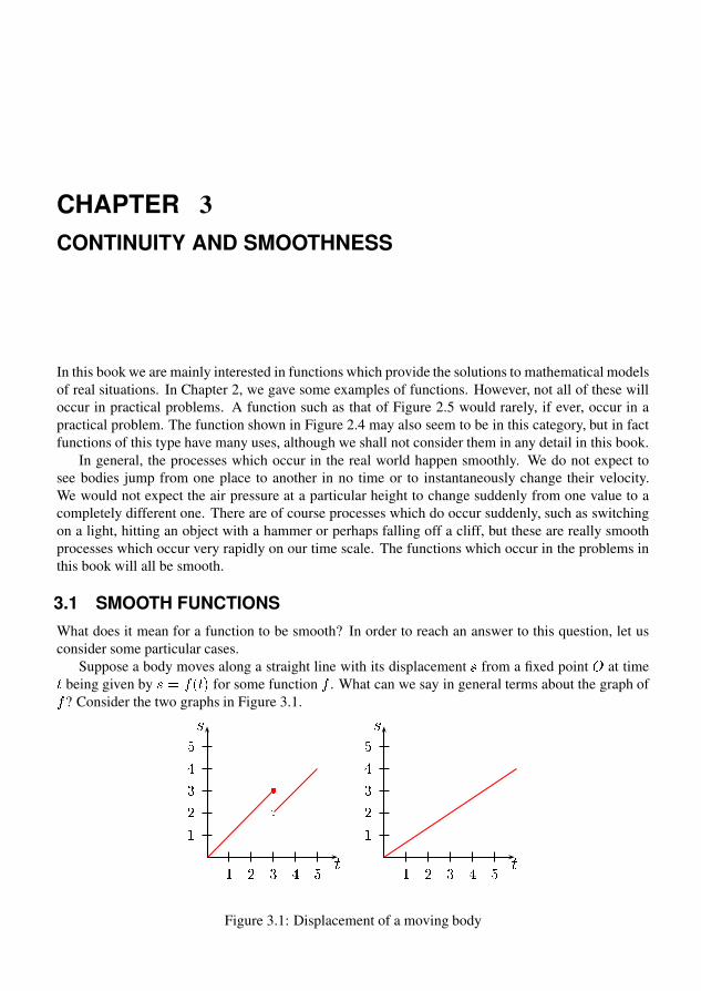
Suppose a body moves along a straight line with its displacement � from a fixed point � at time� being given by � � � � � for some function � . What can we say in general terms about the graph of� ? Consider the two graphs in Figure 3.1.
� � � � ��
� � �
����
� � � � ��
� � �
�Figure 3.1: Displacement of a moving body

28 CONTINUITY AND SMOOTHNESS
Let us look at the figure on the left. For � � � seconds, the graph represents a body which movesaway from � , getting closer to a distance of 3 metres from � as � gets closer to 3 seconds. When� � � , the body is 3 units from � . Immediately after 3 seconds have elapsed the body instantaneouslymoves to a position only 2 metres from � . Clearly, such behaviour is not in accord with our everydayexperience.
The graph on the right is more reasonable. Here the distance from � increases without any suddenchanges in position. The obvious difference between the two graphs is the jump in the first one. Suchdifference in behaviour is described by the notion of continuity: the graph on the right hand side iscontinuous, while the one on the left is discontinuous.
Next, suppose a body moves along a straight line so that its displacement from a fixed point �at time � is given by the graph in Figure 3.2.
� � � ��
��
� �
�
Figure 3.2: Displacement of a moving body
As we have mentioned earlier, the small circle centred at the point � � � indicates that the point atits centre—in this case � � � —is excluded from the graph. The physical interpretation of such a graphis that at the time � � seconds, the body has no position, because there is no point on the –axiscorresponding to the point � � seconds. This behaviour is another example of lack of continuity andis quite unrealistic. We would like to exclude such displacement–time graphs from our considerations.
The essential idea of continuity that emerges from these examples is that the graph of a smoothfunction should have no gaps or jumps.
There is another aspect to the idea of smoothness, which we illustrate by considering two differentcases for the velocity of a moving body. First there is the case where a body moves with constantspeed � in a straight line. If denotes the distance from a fixed point � at time � , then � � � and aplot of against � gives a straight line with slope � . The left hand graph of Figure 3.3 shows the case� � � . Now imagine a body which, at time � � , undergoes an instantaneous change of velocityfrom 0.5 m/sec to 1 m/sec. The right hand graph of Figure 3.3 shows this case. Up to the time � � ,the graph will be a straight line of slope %& . At � � , the graph changes instantaneously to a straightline of slope 1. Such behaviour of moving bodies does not occur in the real world and we want toinvestigate the restrictions needed to rule it out.
The noticeable feature of the right hand graph is the corner at � � . This is what we have to avoidif we are to rule out instantaneous changes in velocity. Loosely speaking, a function is differentiable ifits graph has no corners. We often refer to differentiable functions as smooth functions. We shall latershow that all differentiable functions are continuous, so that a smooth function is one which is bothcontinuous and differentiable. We have at present no way of determining whether or not a functionis differentiable, continuous or neither except to look at its graph. However, a graph constructed

SMOOTH FUNCTIONS 29
� � � � ��
����
� � � � ��
����
�� � � � �
��
���
�
Figure 3.3: Smooth and non-smooth displacements
simply by plotting points is inconclusive, because anything might happen between the plotted points.Figure 3.4 shows an example where the graphs of two functions pass through the same plot points,but one function is smooth while the other is not. To know whether or not a function is smooth, weneed methods which will give conclusive answers and to do this, we will need definitions to tie downthe exact meaning of the concepts of continuity and differentiability.
There is a second reason for needing these definitions. Our main aim is to find the function whichrelates the variables in a practical problem. It turns out that a careful look at the concept of smoothnesswill point the way towards methods for finding such functions.
We should remark that in some applications we need to make use of functions which are notsmooth. The income tax scale is one example. There are also cases where smooth functions changein very short time periods. It is often simpler to approximate such smooth functions by a non-smoothfunction. This may occur when we model the turning of a switch on or off. We will not consider suchapplications in this book.
� � �� �� � �
�
� �
�
� �
� �
�
�
�
Figure 3.4: Two graphs through the same plot points
As is usual in mathematics, we will have to give precise and unambiguous definitions of theconcepts discussed above. Historically, such definitions did not come out of the clear blue sky, or

30 CONTINUITY AND SMOOTHNESS
inscribed on stone tablets. Rather, they developed slowly over time in response to some perceivedneed. Often concepts are taken for granted or are not properly understood, until some example ariseswhich forces us to take more care with their definitions. In our case, there is a need for carefuldefinitions of continuity and differentiability to ensure that the functions we use to describe real worldprocesses are in accordance with experience.
EXERCISES 3.1
1. The square wave function is defined on the interval � � � � � by
� � � � � if � � � � � �� if � � � � � �We extend the definition of
to the entire real line by letting � � � � � � �
for all � " $ . Sketch the graph of
on the interval � % ' � ' � .This function is often used to model a signal generated by repeatedly flicking a switch on andoff. Do you think that the function
is an accurate representation of the physical process?
3.2 CONTINUITYLooking at the graphs of the functions in Figures 2.4, 2.5, 3.1 and 3.2, we see that the jumps or gapsin the graph occur at specific points in the domain and we describe this by saying that continuity isprimarily a point property. A function may be continuous at some points and not continuous at others.In attempting to formulate a precise definition of continuity, we begin with the idea of continuityat a point. There are several criteria—not necessarily independent of each other—which have to besatisfied if a function is to be continuous at some point of its domain. We will motivate such criteriaby considering various examples.
*+� - .
/
0 � 2 � �
Figure 3.5: A graph with a gap

CONTINUITY 31
To begin with, consider the graph of the function � shown in Figure 3.5. In this case, the functionis not defined at the point � � and this is manifested by the gap which appears in the graph above thepoint � � � � . Clearly, the only way to avoid having such a gap is to ensure that there is indeed afunction value at � � , that is, to ensure that � � � is well-defined. This gives us our first criterion forcontinuity.
Criterion 1 In order for a function � to be continuous at a point � � , the number � � � must exist,that is, � � must be in the domain of � .
For our next example, let us consider the function� � given by
� � � � ��������
� if � � � �� � � if � " � � � �� � if � " � � � �) if � * � +The graph of
� � is shown in Figure 3.6. Clearly, we would not want to consider this to be continuousat the point � � � , so that we need a condition that describes this type of jump behaviour. In this
� � ) -. �. ��
�)
0
1Figure 3.6: A jump discontinuity
example, � � � � , while the values of � � for � slightly less than 1 are close to 3 and the values of� � for � slightly greater than 1 are close to 2. There would be no jump if values of � � were closeto 2 (the value of � � ) for all � close to 1. This gives us another criterion for continuity at a point.
Criterion 2 In order for a function � to be continuous at a point � � of its domain, it is necessary thatthe values of � � are close to the value of � � � as long as � is close to � � .
The word “close” is not very precise: how close is “close”? We can sharpen the idea a little bysaying that the values of � � should be arbitrarily close to the value of � � � provided � is sufficientlyclose to � � . However, in our final definition of continuity we will have to be more careful about themeanings of the various terms. For the moment we will continue at an intuitive level.
We can now state a preliminary definition of continuity at a point.

32 CONTINUITY AND SMOOTHNESS
DEFINITION 3.1 Preliminary definition of continuity at a pointThe function � is continuous at the point � � in its domain if:
1. The function � is defined at the point � � , that is, we can compute the number � � � � .
2. The values of � � � are arbitrarily close to the value of � � � � as long as � is sufficiently closeto � � .
The above definition of continuity definition lacks precision, since it makes use of the idea ofsufficiently close. One way to clarify this is to use the idea of a sequence. Loosely speaking, asequence is an infinite list of numbers. Some examples of sequences are given below.
EXAMPLE 3.1(a) � � � � � � � � � �(b) � � � � � � � � � � � �(c) � �� � �� � � � � � �(d) ! $ % � � ! $ ' % � � ! $ ( % � � ! $ � % � � � �
*In order for a sequence to be well-defined, there must be a rule for computing its terms. A sequenceis often referred to by giving the general term in braces. Thus the above four sequences are + , � - ,+ � � / - , + 1 , - and + � $ 1 , / - . Notice that in each sequence there is one term for each positiveinteger and a rule for generating this term from the integer. This leads to a precise definition of asequence.
DEFINITION 3.2 A sequence of real numbers is a function whose domain is the set of positiveintegers. The values taken by the function are called the terms of the sequence.
EXAMPLE 3.2Define a function � by � � , 5 1 , �where , is a positive integer. Then
� � 5 � � � ' 5 �� � � � ( 5 �� � � � � �so � is a sequence and its terms are � �� � �� � � � � � �
*Despite the above definition, a sequence is usually thought of as a list of numbers rather than a
function.The most important property of a sequence is whether or not there is some number � � to which the
terms get arbitrarily close as , gets larger. If this is the case, then the sequence is said to be convergentand the number is called the limit. If the sequence is not convergent, then it is said to be divergent .There are a number of common ways of indicating that the sequence + � / - converges to � � :

CONTINUITY 33
� We may simply state the fact in words: � � � � converges to � .� We may write � � � � as � � � . We read this as � � approaches � as � tends to infinity.� A more compact way of writing the statement above is � � �� � � � � � � .
In simple cases we can determine whether or not the sequence converges by looking at the listof terms. Thus in Example 3.1, the sequence (a) diverges because the terms get larger without anybound, the sequence (b) diverges because the terms oscillate. In each case, there is no number thatthe terms get close to as � gets large. The sequence (c) converges with limit � , since the terms getarbitrarily close to � as � � � . The sequence (d) is more difficult. It is not obvious what happensfrom the terms given. If we compute the decimal approximations of the first few terms we get
2, 2.25, 2.37, 2.44, 2.49, � � �It is still not clear what will happen. There are methods for dealing with such sequences and whilethese are important for many practical purposes we shall not need them in this book. However, thisparticular sequence is important. In Theorem 10.5 of Chapter 10 we will show that it is convergentwith limit 2.71828 � � � , a number commonly denoted by the letter ! . For the present we shall assumethis result without proof, that is, we assume
� � �� � � # $ & ( &� * � , � !� . � 0 & 2 . 2 � � �With the idea of a sequence available, we can improve our understanding of the idea of continuity
of a function 5 at a point � in its domain. If we take any sequence � � � � in the domain of 5 whichconverges to � and then consider the corresponding sequence of function values � 5 8 � � < � , this lattersequence must converge to 5 8 � < if 5 is continuous at � . This is another and more precise way ofstating Criterion 2. Notice that we have implicitly assumed that 5 8 � < exists, which is required byCriterion 1. This property of convergence must hold for every sequence which approaches � , and ofcourse each number in the sequence � � � � must be in the domain of the function, so that � 5 8 � � < � isdefined for all � .
DEFINITION 3.3 Continuous functionsThe function 5 is continuous at the point � in its domain if the sequence � 5 8 � � < � converges to5 8 � < for every sequence � � � � in the domain that converges to � .
Notice carefully the words “for every” in this statement. We must consider input sequences onboth sides of the point � , as well as those which oscillate from side to side. However, to show that afunction is not continuous at a point � , it is enough to find just one sequence � � � � converging to � such that the sequence � 5 8 � � < � does not converge to 5 8 � < .
EXAMPLE 3.3Consider the function ? 8 � < � B � C � D of Example 2.1. To investigate the continuity at � � . , say, weneed to consider input sequences which converge to 2. One of the simplest is � � � � � � . ( & H � � . Theterms are I J . KD J . KL J . KM J � � � J

34 CONTINUITY AND SMOOTHNESS
which converges to � as � tends to infinity. The sequence of function values or output sequence is� � � � � � � � � � � � � � � � � . The terms of this output sequence are� � � � � � � ! � � � � � � $ ! � � � � � � $% � � �The terms in brackets converge to 2, so the output sequence converges to � � � ( � , which is thefunction value at 2.
We have shown that there is a sequence � � � with + , -� / 1 � � � for which + , -� / 1 � � � � 4 � � .
Can we conclude that � is continuous at � � ? Definitely not! The definition of continuity requiresthat the sequence of function values converges to the actual function value for any input sequence,and we have only tried one sequence.
Let’s have another try without tying ourselves down to a particular input sequence such as � � �� � � � . Let � � � be any sequence which converges to 2. Then it is reasonable to suppose that � � �converges to � and hence that � � � � � � converges to � � � ( � . Hence � � � � � converges to � � � .Since � � � can be any sequence converging to 2, we conclude that � is continuous at 2. =In this last example we have made assumptions about the convergence of combinations of sequences.For example, we assumed � � � converges to > if � � � converges to > . There is a theorem whichdeals with these matters. We state it without proof.
THEOREM 3.1Let � � � be a sequence converging to > and let � ? � � be a sequence converging to ? > . Then
(a) � @ � � converges to @ > for any constant @(b) � � � ? � � converges to > � ? >(c) � � F ? � � converges to > F ? >(d) � � ? � � converges to > ? >(e) � � � ? � � converges to > � ? > if ? > G� I and ? � G� I for any � .
This theorem can be proved using a careful definition of convergence of sequences, but we shallnot give the proof here. It is often possible to use this theorem to prove results on continuity, as wewill show below.
EXAMPLE 3.4In order to decide whether or not the sequence
� J � � � K �� � � Mconverges, we note that �� � � � � � � F �� � �� � F �� � � �It should be clear (and this can be proved) that
+ , -� / 1 �� � � � I !

CONTINUITY 35
so that
� � �� � � � � � � �� � � � � � �� � �� �Hence the sequence � � � � converges to 1.
EXAMPLE 3.5Suppose we want to investigate the behaviour of the function given by the rule � ! # % � # ( near thepoint # � + . We may be interested in investigating properties of the function such as continuity ordifferentiability at the point # � + . To this end, it is often useful to take a sequence � # � � convergingto + and see what happens to the sequence � � ! # � % � .
First, note that � ! + % � 6 , so that the function is defined at 3. Next, we choose an input sequencethat converges to 3 from above and see what happens to the corresponding sequence of functionvalues. Let � # � � � 8 + � : �Then � # � � is a sequence converging to 3 from above and we have
� � ! # � % � � ; � + � � ( =� 8 6 � > � ( :? 6 as ? C �
We see that � � ! # � % � ? � ! + % as ? C .Next, we choose an input sequence that converges to 3 from below and see what happens to the
corresponding sequence of function values. Let
� F � � � 8 + � : �Then � F � � is a sequence converging to 3 from above. We have
� � ! F � % � � ; � + � � ( =� 8 6 � > � ( :? 6 as ? C �
We see that � � ! F � % � ? � ! + % as ? C .We have looked at two input sequences, which converge to 3. In both cases the corresponding
function values converge to � ! + % and it seems plausible that � is continuous at # � + , but we have notproved this. K

36 CONTINUITY AND SMOOTHNESS
In the next example, we show how Theorem 3.1 may be used to prove continuity.
EXAMPLE 3.6Let � � � � � � . Show that � is continuous at � � .Solution. To show that a function � is continuous at a point � � , we need to show that the outputsequence � � � � � � � converges to � � � � � for every sequence � � � � which converges to � � .
Let � � � and choose any sequence � � � � � � � converging to 3. Then, by Theorem 3.1 (d)� � � � � � � � � �� � � � � � � � �� � � �so that � � � � � � � � � � � � for any sequence � � � � converging to 3. The conclusion is that � is continu-ous at 3.
EXAMPLE 3.7Show that � � � � � � � ' ) �is continuous at any point � � .Solution. Let � � � � be a sequence converging to � � . Then using Theorem 3.1, � ) � � � converges to ) � �by part (a), � � �� � converges to � �� by part (d), so by part (a) again, � � � �� � converges to � � �� . Hence, bypart (b), � � � �� ' ) � � � converges to � � �� ' ) � � . Since this is true for any input sequence convergingto � � , it follows that � � � � � � � ' ) � is continuous at � � .
EXAMPLE 3.8Define a function � by
� � � � - .../...0
1 if � 3 1 4� if 1 5 � 3 9 4� < 9 if 9 5 � 3 = 4� if � ? = @We shall show that this function is not continuous at � 9 . We do this by taking the input
sequence � 9 < 9 E F � . The output sequence is also � 9 < 9 E F � , which converges to 1. However, thefunction value at � 9 is � � 9 � 1 , so the output sequence does not converge to the function valueand the function is not continuous at � 9 . Notice, however, that if we had taken the input sequence� 9 ' 9 E F � , then the output sequence would have been � � 9 ' 9 E F � < 9 � � 9 E F � , which convergesto 0, so that for this input sequence, the output sequence does converge to the function value. Thisillustrates the fact that we cannot conclude that a function is continuous on the basis of just one inputsequence (or even 1000 input sequences). We can, however, conclude that it is not continuous on thebasis of just one input sequence. Q
These examples illustrate the roles played by definitions and theorems. Definitions provide uswith the concepts and state precisely what we mean by the concepts, but they are not always the besttools to use in practice. We can prove theorems using the definitions and it is these theorems whichprovide the practical tools. Note, however, that the use of definitions can be effective in demonstratingthat a property (such as continuity) does not hold. This happened with Example 3.8.

CONTINUITY 37
EXAMPLE 3.9The function
� � � � � � � � �
� � � � � � � � � �
of Example 2.15 is not continuous at the points � � and 1. This is because these points do not lie in thedomain of the function. No sequence of output values can converge to � � � � � and � � � � , since thesenumbers do not exist.
EXAMPLE 3.10The function
� � � � � � �
� � �
is not continuous at � � , since this point is not in the natural domain of the function. However,when � � we can write
� � � � � � �
� � �
� � � � � � � � � �
� � � � � � $
so that � � � & � converges to 4 for every sequence ( � & * converging to 2. Hence if we define � � � � to be4, then � is continuous everywhere, including the point � � . .
It is not hard to see that every polynomial function is continuous at every point of its domain. Suchfunctions illustrate the idea of continuity on an interval.
DEFINITION 3.4 Continuity on an open intervalA function which is continuous at every point of an open interval / is said to be continuous on / .
It is also possible to define continuity on closed intervals.
DEFINITION 3.5 Continuity on a closed intervalA function � is continuous on the closed interval 0 1 $ 3 5 in its domain if:
1. � is continuous on the open interval � 1 $ 3 � .
2. For every sequence ( � & * in 0 1 $ 3 5 converging to 1 , the sequence ( � � � & � * converges to � � 1 � .
3. For every sequence ( � & * in 0 1 $ 3 5 converging to 3 , the sequence ( � � � & � * converges to � � 3 � .
It should be clear how to define continuity on intervals such as 0 1 $ 3 � or � 1 $ 3 5 and we leave thisas an exercise. A function which is continuous on an interval / (closed, open or neither) is said to becontinuous on / . A function which is continuous at all points of its domain is simply referred to asbeing a continuous function . Thus polynomials are continuous functions.
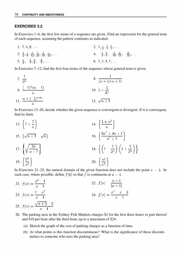
38 CONTINUITY AND SMOOTHNESS
EXERCISES 3.2
In Exercises 1–6, the first few terms of a sequence are given. Find an expression for the general termof each sequence, assuming the pattern continues as indicated.
1. � � � � � � � � � 2. � � � � � � � � � � �3. � � � � � � � � � � � � � � � � � � 4. � � � �� � � � � � �� � � � �� � � � � �5. � � � �� � �� � � �� � � � � 6. � � � � � � � � � � �
In Exercises 7–12, find the first four terms of the sequence whose general term is given.
7.�� � 8.
�� � � � � � � � # �9.
� � � � � � � � � �� 10. � � �# �11.
� � � � � � � * � 12. + � � �In Exercises 13–20, decide whether the given sequence is convergent or divergent. If it is convergent,find its limit.
13. , � � �� .14. , � � � �� .
15. 1 + � � � � + � 2 16. , # � � � � � � �� � � � .17.
5 7 # �� � � 818. , 9 � � �# � ; 9 � � �# � ; .
19. , � �� � .20. , � >� � .
In Exercises 21–25, the natural domain of the given function does not include the point ? A � . Ineach case, where possible, define C � � � so that C is continuous at ? A � .
21. C � ? � A ? � � �? � � 22. C � ? � A ? � �I ? � � I23. C � ? � A � � ? �? � � 24. C � ? � A ? � � ? � �? � �25. C � ? � A + ? � # � �? � �26. The parking area in the Sydney Fish Markets charges $2 for the first three hours or part thereof
and $10 per hour after the third hour, up to a maximum of $24.
(a) Sketch the graph of the cost of parking charges as a function of time.
(b) At what points is this function discontinuous? What is the significance of these disconti-nuities to someone who uses the parking area?

CONTINUITY 39
27. Let � be the function defined by the rule
� � � � � � � � � �� � � � � � � �Draw the graph of � . It should be clear from your graph that � is not continuous at � � . Toverify this you need to find a sequence � � � which converges to 2, but for which � � � � � � doesnot converge to � � � � ' . Show that � � � � * , is such a sequence. What does � � � � � � * , � converge to? Find a sequence � � � for which � � � � � � converges to 4.
28. Two important functions in science and engineering are the Heaviside function / 1 , defined by
/ 1 � 4 � 7 � 4 9 ;� � 4 < ;for any ; > ? , and the unit pulse function @ A C 1 , defined by@ A C 1 � 4 � D A E / 1 � 4 � F / 1 I A � 4 � Lfor any ; � N > ? . Draw the graph of each function and determine where the functions arecontinuous.
29. Let / 1 be the Heaviside function defined above. Draw the graphs of / � � 4 � , / � � � � 4 � and/ S D � F 4 � .
30. Explain how we can define continuity of a function on intervals such as E ; � U � or � ; � U L .For each sequence � � � of input numbers in Exercises 31–35, find the corresponding sequence ofoutput numbers � � � � � � for the functions indicated.
31. � � � W X � �, Y � � � � � [ � � � 32. � � � W X F �, Y � � � � � [ � � �33. � � � W � F �, Y � � � � � � ^ 34. � � � � � � � � � �35. Show that the function defined by � � � � X � � is continuous at � b .
36. Show that the function defined by � � � � X � � is continuous at � � c .
37. Show that the function defined by
� � � � � � � � � �b F � � � � �is not continuous at � � .
38. Show that the function � � � � � if � 9 �� F � if � < �is continuous on each of the intervals � F f � � � and E � � f � , but not on the interval � 7 � � � .

This page intentionally left blank

CHAPTER 4DIFFERENTIATION
In Chapter 2, we informally discussed continuity and differentiability. In Chapter 3, we introducedprecise definitions for continuity and we must now do the same for differentiability. In Chapter 2, weinformally defined a function to be differentiable at a point if its graph has no corner at that point. Inthis chapter, we present a more detailed discussion of differentiability.
4.1 THE DERIVATIVELet � be a given continuous function and let � � be a point in its domain. To investigate the differen-tiability at the point � � , first take a point � � � � � in the domain of � (Figure 4.1). The gradient of thesecant
� �joining the points � � � � � � � � � � and � � � � � � � � � � is given by
� � � � � � � � � � � �� � � � �
!
"
� � � ��
� � � � �� � � � �
�
Figure 4.1: A secant of a graph
If we take an input sequence # � � % which converges to � � then for each point � � we can take asecant joining � � � � � � � � � � and � � � � � � � � � � . The gradients of such secants form a sequence
' � � � � � � � � � � �� � � � � ( (4.1)

42 DIFFERENTIATION
There are some minor sources of difficulty which we need to dispose of. In the first instance, wenote that it is quite possible to choose a sequence � � � � which converges to � � and for which � � � �for at some positive integer � , in which case the corresponding quotient in the sequence (4.1) willbe undefined. To avoid this happening, we shall restrict ourselves to sequences � � � � which have theproperties � � � � � as � � � and � � �� � � for all positive integers � . Such sequences will be calledspecial sequences converging to � � .
In order for there to be sequences � � � � � � � with � � �� � � , we shall require that � be defined onan open interval about � � .
If � � is in the domain of a function � , and if � � � � is any special sequence converging to � � , thenseveral different things may happen:
� The sequence (4.1) may diverge for some (perhaps every) choice of � � � � .
� The sequence (4.1) may converge to a number which depends on the choice of � � � � .
� The sequence (4.1) may converge to the same number for every possible choice of � � � � .
From a graphical point of view, it appears that if the sequence (4.1) of gradients of secants converges,then it will converge to the gradient of the tangent at � � .
EXAMPLE 4.1In the table, we have computed the sequence (4.1) for � � � ! � � $ , � � � & and � � � � � � & * + , � � .
� 1 2 5 10 100 1000
� � 3 2.5 2.2 2.1 2.01 2.001. � � � � ! / � � & ! 4 , � � � / & ! 19 15.25 13.24 12.61 12.0661 12.0067
This table suggests (but does not prove) that
7 8 9� : < � � � � ! / � � & !� � / & � + & ? @
A � �� �
B
C
Figure 4.2: A nonsmooth graph

THE DERIVATIVE 43
EXAMPLE 4.2Consider the function whose graph is given in Figure 4.2, which has a corner at � � . It is interestingto see how this corner manifests itself in terms of the gradients of secants. Firstly, if we take asequence � � � � for which each � � � � � and which converges to � � , then the diagram suggests thatthe gradients of the corresponding secants will converge to a negative number. On the other hand, ifwe take a sequence � � � � with each � � � � � and which converges to � � , then the diagram suggeststhat the gradients of the corresponding secants will converge to a positive number. Clearly, the twogradients will not then converge to the same number.
EXAMPLE 4.3Let us define the function � by the rule � � � � � � � . This is a function whose graph we would certainlyexpect to satisfy our intuitive notion of a smooth function. In Example 4.1 above, we estimated thegradient at a point on the graph of � � � by drawing up a table, but such a table cannot give anexact answer for the gradient at a particular point. In this example, we will use what we know aboutconvergence of sequences to get an exact answer for the gradient of the tangent at a particular pointon the graph.
Let � � be any real number (so that � � is in the domain of � ). Choose any input sequence � � � �converging to � � . We then have
! � � � � � # � � � � �� � # � � ' � ! � �� # � ��� � # � � '� ! � � � ) � � � � � � # � � �� � # � � '� � � � ) � � �
and this sequence clearly converges to 0 � � independently of the choice of the sequence � � � � . Noticethat � � # � � can be cancelled, because for every 1 , � � # � � 3� 5 6EXAMPLE 4.4Here is an example of a function which we do not expect to be smooth. Let � � � � � 8 � 8 , that is, let
� � � � � 9 # � < � � 5� � @ 5The graph has a corner at � � 5 , so let us investigate the sequence
! � � � � � # � � � � �� � # � � '(4.2)
for the case � � � 5 . First take a decreasing input sequence � � � � � � F G 1 � . This input sequenceconverges to 5 . The output sequence (4.2) corresponds in this case to
! � � � � � # � � 5 �� � # 5 ' � ! � � F G 1 � # � � 5 �F G 1 # 5 '� ! F G 1 # 5F G 1 # 5 ' <

44 DIFFERENTIATION
�
�
� � � � � � �
� � �� � �� �� �� � ��
�
Figure 4.3: The graph of � � � � � � �which converges to � . On the other hand, the increasing input sequence � � � � � ! � $ & � also con-verges to ' , but the corresponding output sequence is
( � � � � � ! � � ' �� � ! ' 0 ( � � ! � $ & � ! � � ' �! � $ & ! ' 0 ( � $ & ! '! � $ & ! ' 0 5
which converges to ! � . In this example the presence of the corner has caused different output se-quences to converge to different numbers, even though the corresponding input sequences both con-verged to � ' . 8DEFINITION 4.1 Differentiable functionsLet � be a function which is defined at all points of an open interval 9 . The function � is differen-
tiable at � ; = 9 if the sequence
( � � � � � ! � � � ; �� � ! � ; 0(*)
converges to the same limit for every special sequence � � � � converging to � ; , where � � = 9 for all& . This limit is normally denoted by the symbol � B � � ; � .
Notice that the statement that the sequence
( � � � � � ! � � � ; �� � ! � ; 0converges to � B � � ; � can be written as
D E F� G H � � � � � ! � � � ; �� � ! � ; � B � � ; � JThis definition says nothing about the interpretation of the value of the limit. From a graphical
point of view, as � � gets close to � ; , the terms of the sequence (*) in Definition 4.1 get close to thegradient of the tangent at � ; for a function with no corner. We expect the limit of the sequence to bethe slope of the tangent at � ; . A function with no corner at � ; has a unique tangent, while if there isa corner, then there is not a unique tangent.

THE DERIVATIVE 45
DEFINITION 4.2 The derivativeThe number � � � � � is called the derivative of the function � at the point � . This enables us todefine a new function (denoted by � � ) called the derivative of � according to the rule � � � � � � � � ,where � is any point in the domain of � at which � is differentiable. The domain of � � is the set ofall points where � is differentiable.
Notice that since � � is a function, it may also be differentiable. If this is the case, we denote itsderivative by � � � and call it the second derivative of � . In the same way we can define third, fourthand higher derivatives.
EXAMPLE 4.5Suppose � � � � � � . Let � � � � be a sequence converging to a point � � . Then� � � � � ! � � � �� � ! � � � � ! � � � ! � � & (so that the sequence ) � � � � � ! � � � �� � ! � +is just the sequence � & ( & ( & ( . . . � which converges to & . Thus � � � � � � & .
EXAMPLE 4.6If � � � � � � 1 , then according to the calculations in Example 4.3, � is differentiable at all points of itsdomain and � � is the function with domain given by the rule � � � � � � 3 � .
EXAMPLE 4.7If � � � � � 5 � 5 , then � is differentiable at all points of its domain, except for the point � � 7 , so that � �has domain ! � 7 � and � � � � � � ; ! & if � > 7& if � @ 7 . (4.3)
We leave you to prove this result as an exercise. AThe derivative of a differentiable function is one of its most important properties. If we are given
some function, then the derivative can often tell us a great deal about the behaviour of the functionand may assist in sketching its graph. There is a more important aspect to the derivative, however.In many problems we find that the natural formulation of the problem gives us information about thederivative of the solution function rather than information about the function itself; we have to usethe derivative to calculate the solution function. This method of solving problems by first finding thederivative and then using this derivative to find the solution function is the basis of calculus. It wasdiscovered about 300 years ago by Sir Isaac Newton and Gottfried Leibniz.
The definition we have given for the derivative of a function expresses precisely what we meanby a function having no corners in its graph. We can use this definition to calculate the derivative ina few simple cases, but it is not a very efficient method compared with those which we shall shortlydevelop. Using the definition to find derivatives is known as differentiation by first principles. In thisbook, we use differentiation by first principles in the following two instances:B To aid in the understanding of the definition

46 DIFFERENTIATION
� To prove theorems which enable us to use more efficient methods of calculating derivatives.
A process based on differentiation by first principles also occurs in some numerical work. Whenmeasuring a variable quantity such as a seismic signal, we may only have its values at discrete pointsin time. To calculate the time rate of variation, we have to approximate the derivative by the slope ofa chord joining two nearby data points. This is the basis of finite difference methods.
4.1.1 Remarks on notation
Before going on to develop efficient rules for differentiation, we need to consider some matters ofnotation. All of the functions we have discussed have been denoted by a single letter such as � , � or�
. We can regard such a letter as the name of the given function. Of course, we don’t have to restrictourselves to single letters for function names. We could, for instance, define a function ‘step’ by therule
step � � � � � � � � � � � �Some functions have names which are universally agreed upon. You have probably met some of thesebefore. Common examples are � � � � � , � � � � and # $ � � , usually written as � � � � , � � � and # $ � .We don’t even have to use letters, for example the square root function is denoted by the specialsymbol ( and the output number corresponding to the input number � is denoted by ( � .
Many simple functions do not have universally agreed names and are defined by algebraic formu-las, for example polynomials such as
� � � � � + , � . / 1 � , � �Indeed, we often only refer to the formula in speaking of the function. Thus we (incorrectly) speak ofthe function � + , � . / 1 � , � , when we really mean the function whose output number is � + , � . / 1 � , �when the input number is � . Function values in such cases are denoted by a vertical stroke notation:
� � + , � . / 1 � , � 7 8 : ; < � > � > �This means the same thing as � � � if � � � � � + , � . / 1 � , � . Mathematica uses a similar notation.If we want to substitute � � � in the expression � + , � . / 1 � , � , then the Mathematica expressionis
xˆ3-xˆ2+2x-1/.x->10
Another notation is often used in applications where there are independent and dependent variables.If the values of the independent variable are denoted by � and those of the dependent variable byJ and if the function is defined by a formula such as � . , then we write J � � . and say that J is afunction of � . Particular values of J are denoted by the function value notation. Thus J � O � O . � > .The derivative is written J Q and this again denotes a function with particular values written with thefunction value notation, as in J Q � 1 .
There is also an alternative notation for derivatives which originated with Leibniz and which isstill used today—the S J U S � notation. Recall that the derivative of a function � at a point � < is
� Q � � < � # � WX Y [ � � � X , � � � < � X , � < �where ^ � X _ is any special sequence that converges to � < . Let us put J � � � � . Leibniz wrotea � � � X , � < and
a J � � � � X , � � � < and considered the quotienta J U a � . As d f h this
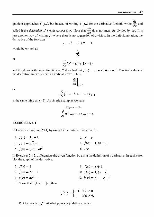
THE DERIVATIVE 47
quotient approaches � � � � � , but instead of writing � � � � � for the derivative, Leibniz wrote � � and
called it the derivative of � with respect to � . Note that � � does not mean � divided by � . It is
just another way of writing � � , where there is no suggestion of division. In the Leibniz notation, thederivative of the function � � � � � � � � � � � �would be written as � �or � � � � � � � � � � � � �and this denotes the same function as � � if we had put � � � � � � � � � � � � � � � . Function values ofthe derivative are written with a vertical stroke. Thus � � &&&& ' ) �or � � � � � � � � � � � � � + ' ) �is the same thing as � � � � � . As simple examples we have� � + ' ) � � - / � � � + ' ) � � � � + ' ) � � 0 1EXERCISES 4.1
In Exercises 1–6, find � � � 2 � by using the definition of a derivative.
1. � � � � � 4 � � � 2. � � � �3. � � � � � 6 � � � 4. � � � � � � 9 � � � � �5. � � � � � � � � � 2 � � 6. � 9 �
In Exercises 7–12, differentiate the given function by using the definition of a derivative. In each case,plot the graph of the derivative.
7. � � � � � 2 8. � � � � � � � �9. � � � � � 2 � � � 10. � � � � � � 9 � � � � �
11. > � � � � � � � � � 12. @ � � � � � � � 4 � � �13. Show that if � � � � � + � + , then
� � � � � � D � � if � G H� if � I H 1Plot the graph of � � . At what points is � � differentiable?

48 DIFFERENTIATION
14. Decide which, if either, of the two functions � � � � � � � � and � � � � � � � is differentiable at� � ; justify your answers.
In Exercises 15–18, draw the graph of the derivative of the given function.
15. 16.
�
�
�
�
17. 18.
�
�
�
�
19. Let � be a differentiable function and let be a small positive number. Give a physical meaningto the quotient
� � � � � � � � � �
in the following cases.
(a) � � � � is the height of a missile � seconds after liftoff.
(b) � � � � is the population of a city at time � .
(c) � � � � is the cost in dollars of producing � units of a product.
4.2 RULES FOR DIFFERENTIATIONWe have identified the derivative of a differentiable function as one of its important properties. As yet,we have no way of calculating the derivative, except by the use of Definition 4.1 on page 44, which isoften a cumbersome process. In this section we will develop more efficient computational proceduresfor evaluating derivatives.
The functions we have already met have often been combinations of simpler functions. For in-stance, the function
� � � � � � � � � � � � � � " � �
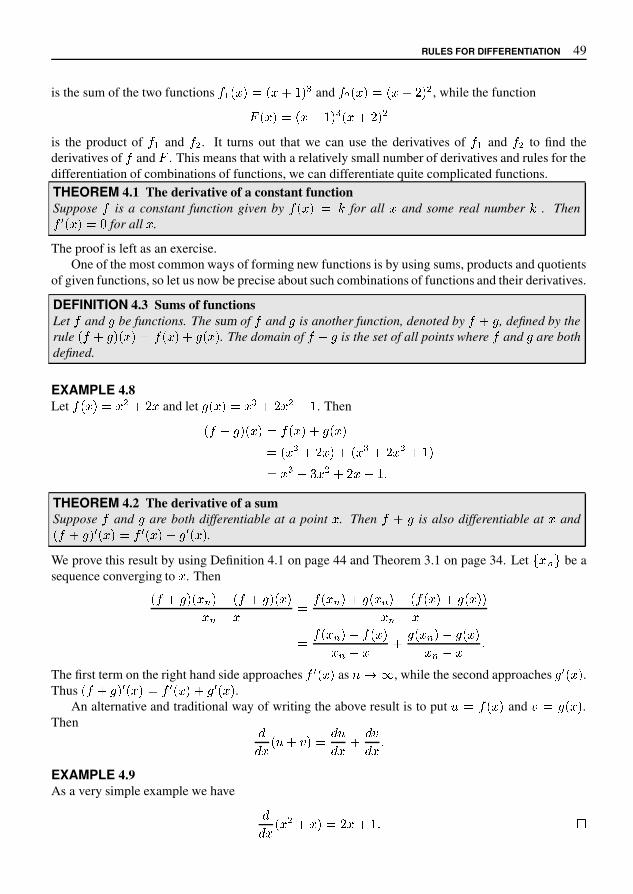
RULES FOR DIFFERENTIATION 49
is the sum of the two functions � � � � � � � � � � � and � � � � � � � � � � � , while the function� � � � � � � � � � � � � � � �
is the product of � � and � � . It turns out that we can use the derivatives of � � and � � to find thederivatives of � and
�. This means that with a relatively small number of derivatives and rules for the
differentiation of combinations of functions, we can differentiate quite complicated functions.
THEOREM 4.1 The derivative of a constant functionSuppose � is a constant function given by � � � � � for all � and some real number � . Then
� � � � � � for all � .
The proof is left as an exercise.One of the most common ways of forming new functions is by using sums, products and quotients
of given functions, so let us now be precise about such combinations of functions and their derivatives.
DEFINITION 4.3 Sums of functionsLet � and � be functions. The sum of � and � is another function, denoted by � � � , defined by therule � � � � � � � � � � � � � � � � � . The domain of � � � is the set of all points where � and � are bothdefined.
EXAMPLE 4.8Let � � � � � � � � � and let � � � � � � � � � � � � . Then
� � � � � � � � � � � � � � � � � � � � � � � � � � � � � � � � � � � � � � 0 � � � � � � � 2
THEOREM 4.2 The derivative of a sumSuppose � and � are both differentiable at a point � . Then � � � is also differentiable at � and
� � � � � � � � � � � � � � � � � � � � .
We prove this result by using Definition 4.1 on page 44 and Theorem 3.1 on page 34. Let 6 � 8 9 be asequence converging to � . Then
� � � � � � � 8 � < � � � � � � � �� 8 < � � � � 8 � � � � � 8 � < � � � � � � � � � � �
� 8 < �
� � � 8 � < � � � �� 8 < � � � � � 8 � < � � � �
� 8 < � 2
The first term on the right hand side approaches � � � � � as ? @ B , while the second approaches � � � � � .Thus � � � � � � � � � � � � � � � � � � � � .
An alternative and traditional way of writing the above result is to put D � � � � and F � � � � .Then
HH � � D � F � H D
H � � H FH � 2
EXAMPLE 4.9As a very simple example we have
HH � � � � � � � � � � � 2 I

50 DIFFERENTIATION
We can also define scalar multiples of functions: if � is any real number and � is any givenfunction, then � � is the function defined by
� � � � � � � � � � �It has the same domain as � . For example if � � � � then � � is the function given by the rule �� � � . It is easy to verify that, for any real number � ,
� � � � � � � � � � � �and you should do this as an exercise.
We can summarise the two rules we have so far:
� The derivative of a sum is equal to the sum of the derivatives.
� The derivative of a scalar multiple of a function is the same scalar multiple of the derivative ofthe function.
Unfortunately, the results for products and quotients do not follow such a simple form. First adefinition:
DEFINITION 4.4 Products and quotients of functionsLet � and � be two functions.
� The product of � and � is the function � � defined by the rule � � � � � � � � � � � � . Theproduct is defined at all points where � and � are both defined.
� The quotient of � and � is the function� � defined by the rule
# � � $ � � � � �� � � �The quotient is defined for all points where � and � are both defined and where � � � & ' .
EXAMPLE 4.10Let � � � � and let � � � � * , . Then
� � � � � � � � � * , � �The domain of both � and � is . , so that the domain of � � is also . .
As for the quotient of these functions, we have
# � � $ � � � � * , �The domain of the quotient function is . 0 1 * , 4 , 7 . 8THEOREM 4.3 The derivative of a productSuppose � and � are both differentiable at a point . Then the product � � is also differentiable at and � � � � � � � � � � � � � � ; � � � � � � � .

RULES FOR DIFFERENTIATION 51
To justify this result, we take a point � in the domain of � � and an input sequence � � � convergingto � . Then we must consider the sequence whose general term is
� � � � � � � � � � � � � � � �
� � � ��
� � � � � � � � � � � � � � � � � � �
� � � �� (4.4)
The aim of the game is to write the left hand side of equation (4.4) in terms of
� � � � � � � � � �
� � � �
and� � � � � � � � � �
� � � ��
since these terms converge to � � � � � and � � � � � respectively. There is a trick used here: subtract andthen add the term � � � � � � � � � in the numerator of equation (4.4). This gives
� � � � � � � � � � � � � � � �
� � � ��
� � � � � � � � � � � � � � � � � � � � $ � � � � � � � � � � � � � � � � � �
� � � �
�� � � � � � � � � �
� � � �� � � � � $
� � � � � � � � � �
� � � �� � � � � (4.5)
Now as ' ) + ,� � � � � � � � � �
� � � �) � � � � �
and� � � � � � � � � �
� � � �) � � � � � �
but what does � � � � � approach as ' ) + ? We know that if � is continuous at � , then � � � � � ap-proaches � � � � as � � approaches � , but how can we assume that � is continuous at � ? Well, it is truein general that if a function is differentiable at a point � then it is automatically continuous there. Infact
� � � � � �� � � � � � � � � �
� � � �� � � � � � $ � � � �
) � � � � � 3 5 $ � � � �
� � � � � �
where we have used Theorem 3.1. Thus the right hand side of equation (4.5) approaches � � � � � � � � � $� � � � � � � � � and this is the derivative of � � � � � � � . 7
Theorem 4.3 can be written in Leibniz notation as
8
8 �� : ; � � :
8 ;
8 �$ ;
8 :
8 ��
where : � � � � � and ; � � � � � . Note that the derivative of the product is not the product of thederivatives. The correct rule, as given by Theorem 4.3 is an inevitable consequence of the definitionof the derivative and its interpretation as the slope of the tangent or (as we shall see in the next section)as a rate of change.

52 DIFFERENTIATION
EXAMPLE 4.11We have
�� � � � � � �� � � � � � � � �� � � � � �� � � � � � � � � � � � �
the same result we obtained earlier by first principles. Next we have
�� � � � � � �� � � � � � � � � � �� � � � � �� � � � � � � � � � � � � � � � �
and in general �� � � � ! � " � ! % & ' (The last result in the above example is an important one and is worth highlighting.
THEOREM 4.4If " is a positive integer and ) � � � � ! for � + - , then ) . � � � " � ! % & .
There are a number of ways of proving this result. One way has been suggested in the above exampleand another method is outlined in Exercise 4.2.
Finally, we state the rule for differentiating a quotient. This rule can be proved along the samelines as for a product, but we shall not present the proof here.
THEOREM 4.5 The derivative of a quotientSuppose ) and 0 are both differentiable at a point � and suppose 0 � � � 2 4 . Then the quotient ) 6 0
is also differentiable at � and
8 ) 0 9 . � � � ) . � � � 0 � � � < ) � � � 0 . � � �0 � � � � 'This result can be written in the Leibniz notation as
�� � > ? @ A @ ? . < ? @ .@ � �where ? ) � � � and @ 0 � � � .
With the results in this section, we can differentiate any function defined by an algebraic formulawithout having to go back to the original definition. We can do this because we have proved sometheorems. The purpose of theorems is to simplify calculations. We had to use the original definition inthe proofs of the theorems, but once we have proved the theorems we no longer have to differentiateby first principles. Of course, if we encounter a new function which is not simply a combination ofknown ones, then we would have to go back to the definition to find its derivative.

VELOCITY, ACCELERATION AND RATES OF CHANGE 53
EXAMPLE 4.12Let � � � � � � � �Then
� � � � � � � � � �� � � � � � � �� � � � � �� � � � � � � � � � � � � � � � � �� � � � � � �� � � � �EXERCISES 4.2
In the following Exercises, differentiate the given function using the theorems in Section 4.2.
1. � � � � � � � � 2. � � � � � � ! � � � � 3. � � � � � � 4. � � � � � � � � � � � � �5. � � � � � � �� � 6. � � � � � ' � ( � � � � � � � �7. Show that if � � � � + for all � , where + is some constant, then � � � � � - .
8. Here is an outline of a proof that if � � � � � 0 , then � � � � � 2 � 0 5 6 , where 2 is a positiveinteger. Begin by checking that
7 0 � 9 0 � 7 � 9 � � 7 0 5 6 � 9 7 0 5 � 9 7 0 5 ! � ; ; ;; ; ; � 9 0 5 ! 7 � 9 0 5 7 � 9 0 5 6 �for any real numbers 9 and 7 and any positive integer 2 . Next, let > � � A be an arbitrary sequencewhich converges to � . Show that� � � � � � � � � �� � � � � 0 5 6� � � � 0 5 � � ; ; ; � � 0 5 ! � � � � 0 5 � � � � 0 5 6 Eand hence that the sequence
F � � � � � � � � � �� � � � Gconverges to 2 � 0 5 6 .
9. Use Theorem 4.5 to show that if � � � � � 0 , then � � � � � 2 � 0 5 6 , where 2 is a negative integer.
4.3 VELOCITY, ACCELERATION AND RATES OF CHANGEHistorically, the derivative first explicitly appeared in connection with the motion of bodies. This wasan innovation by Sir Isaac Newton who, in the period 1665–1667, laid the foundations of the calculus.

54 DIFFERENTIATION
Newton was interested in the mechanics of motion, particularly the motion of the planets around thesun, which involved velocity and acceleration. He restricted his attention to derivatives with respectto time, which he called fluxions. His notation of
�� for � � � � � is still widely used today.
4.3.1 VELOCITY
Suppose a particle moves along a straight line in such a way that its distance � from a fixed point attime � is given by � � � � � , where is a smooth function. In general the velocity at which the particlemoves will vary as the time changes and we may wish to find the velocity at a particular time � � , say.We can do this in the following way. First take a special sequence � � � � which converges to � � . Forany particular value of � , the average velocity between the time � � and the time � � is given as
average velocity � distance movedtime taken� � � � � � � � � �� � � � � #
As we let � get arbitrarily large, the time interval � � � � � will decrease and we expect that the se-quence of average velocities will converge. The number to which it converges is defined to be theinstantaneous velocity at the time � � . But the number to which the sequence
& � � � � � � � � �� � � � � 'converges is just ( � � � � , so that at the time � � , the velocity * is given by* � ( � � � � #4.3.2 RATES OF CHANGE
In the case of a straight line - � / � 1 � , the slope / of the line gives the rate of change of - withrespect to � . If � changes by an amount
2 � then the corresponding change2 - in - is / times as
much, that is,2 - � / 2 � . The sign of / is significant. If it is negative, then - decreases as �
increases, while if it is positive, then - increases as � increases.In the more general case of a differentiable function - � � � � , we can proceed in a similar way
to which we did in the case of velocities. We define the instantaneous rate of change of - with respectto � at the point � � by ( � � � � . If - is increasing at � � , then the rate of change is positive, while if -is decreasing at � � , the rate of change is negative. As an example, velocity is the rate of change ofdistance with respect to time.
EXAMPLE 4.13A screen saver consists of expanding squares which appear at random points on a computer screen. Ifthe length of side � of each square increases in length with a speed of 2 cm/sec, find the rate of changeof the area of a given square when its side length is 6 cm.Solution. The area
8of a given square is given by8 � � 9� : � 9 ;
since � � = � at time � . Consequently, 8 ( � � � � ? � #

VELOCITY, ACCELERATION AND RATES OF CHANGE 55
Since � � � when � � , we compute � � � � � � . Hence the rate of change of area with respect to
time is 24 cm � /sec.
4.3.3 ACCELERATION
Finally we consider the concept of acceleration. If a particle has a velocity � � at time � � and a velocity� � at time � � , then the average acceleration during the time interval � � � � � is defined to be
� � � � �� � � � � �By using a similar argument to the above, we define the instantaneous acceleration � at a time � � to be
� � � �� � " """� �
� $ � � � � � �The acceleration is the rate of change of velocity with respect to time.
EXERCISES 4.3
Exercises 1–4 refer to a body which moves along the � axis in such a way that its position at time � isgiven by � � � � � � .
1. Find the average velocity of the body over the time interval * � � , � � . 0 2 .2. Tabulate the average velocities over the time intervals * � , � . 0 2 , for 0 � 9 , : � 9 , : � : 9 and : � : : 9
seconds.
3. Use the results from Exercise 2 to guess the instantaneous velocity at � � � .
4. Let ; 0 = ? be any sequence converging to zero. Confirm your guess in Exercise 3 by finding thelimit of the average velocities over the time intervals * � , � . 0 = 2 , B � 9 , � , � , � � � , E .
5. If an object has fallen a distance of � � F � � metres after � seconds, what is its velocity after 4seconds?
6. The distance H of a particle from a fixed point at time � is given by
H � � I � F � � . 9 L � �At what times is the velocity zero? What is the acceleration at these times?
7. Find the rate of change of the area of a circle with respect to the radius. What is this rate ofchange when the radius is 3 m?
8. Find the rate of change of the area of a square with respect to the length � of one of its diagonals.What is the rate of change when � � � ?
9. A pebble is dropped into a pond at time � � : , where � is measured in seconds. This causes acircular ripple that moves out from the point of impact at 2 m/s. At what rate (in m � /s) is the areawithin the circle increasing when � � L ?
10. Show that the rate of change of area of a circle with respect to its radius is equal to its circumfer-ence.
11. Show that the rate of change of volume of a sphere with respect to its radius is equal to its surfacearea.

56 DIFFERENTIATION
12. Show that the rate of change of volume of a cube with respect to the length of its edge is equalto half its surface area.
13. The distance � (in metres) of a car from a fixed point at time � (in seconds) is given in thefollowing table.
� 0 1 2 3 4 5 6 7 8 9 10 11 12
� 0 1.2 4.7 10.6 19.3 30.0 43.2 58.6 75.6 97.2 118.8 140.4 162.0
Find the average velocity during the time interval � � � � . Estimate the velocity and acceler-ation at � � � s. Over which period of time is the car moving with constant velocity?
14. The elevation of the Parramatta River � km from its source near Parramatta is given by � � � forsome function . What is a reasonable domain for ? What can you say about the sign of � � � � ?
15. The following graph shows the percentage of alcohol� � � � in the blood of a person as a function
of time � in hours since drinking two double whiskies. What was the approximate rate of increasein the percentage of alcohol in the blood after half an hour? At approximately what rate was theperson eliminating alcohol after four hours? The legal blood limit in most states in Australiais 0.05%. When could this person legally drive home? [From Petocz, Petocz and Wood, IntroductoryMathematics, Thomas Nelson, Melbourne, 1992.]
� � � � �
� � �
� � � �
� � �
�
� � � �
16. Newton’s law of gravitation states that when a spaceship is at a distance from the centre of theearth, its weight
�is given by
� �� !
" # $where
!is the mass of the earth, " is the mass of the spaceship and
�is a constant, known
as the gravitational constant. Find the rate of change of�
with respect to and show that it isnegative. What is the physical meaning of this result?
CHAPTER 5FALLING BODIES
We now have enough mathematical machinery available to solve the first of the problems posed inChapter 1, that of falling bodies. In this chapter, we examine the motion of bodies moving underthe influence of gravity. Here are a few of the cases where the mathematics needed for this type ofproblem is used:
� In the Tower of Terror described in Chapter 1
� In the motion of rockets and missiles
� In designing artillery
� In some movie stunts.
We have already set down the requirement that the solution to any of the problems we will considerin this book should be a smooth function, that is, a function which is continuous and differentiable.So far the only functions we have considered are those defined by algebraic formulas. There are threemain types:
� Power functions of the form � � � � � � , where is an integer. For example � � � � � � or� � � � � � � .
� Polynomials, which are the sums of positive integer power functions. For example � � � � � � � � � � � � or � � � � � " # .
� Rational functions, which are quotients of polynomials. For example � � � � � � " � � �
� � � � � � �&
Such functions are differentiable at all points of their domain, which in the case of a rational functionis the set of all points for which the denominator is not zero. Thus in searching for a solution to apractical problem, the first place we might look is among functions of the above types.
5.1 THE TOWER OF TERRORSuppose, as in the Tower of Terror, we project a body upwards from some point on or above theEarth’s surface and observe it rise, stop at its highest point and then fall. Let ' be the height above theground and let ( be the time. We are seeking a function � such that ' � � ( � . The rule defining � will

58 FALLING BODIES
tell us how to calculate values of � from values of � . Notice the role played by the various symbols: �is a number which is calculated from another number � by the application of a rule � . This is what wehave to do if we wish to keep things strictly correct. However, what is correct and what is convenientmay sometimes be two different things. In what follows, it will be more convenient to write � � � �instead of � � � � . The symbol � is thus doing double duty. It may denote either a number or the rule forcalculating this number. Mathematicians have introduced special terminology to describe such cases.They call it abuse of notation , as in “by abuse of notation, let us write � � � � for � � � � ”.
The problem we are considering is a very old one. Throughout recorded history, people havebeen hurling objects through the air, usually at each other. It was regarded as important to understandmatters such as the flight of arrows or cannonballs. The theory is now well understood, but this was notalways the case. There were many misconceptions about the laws governing the motion of projectilesand it was not until the 17th century that Galileo finally developed the theory that we use today. Sincewe now know how to predict the path of projectiles we could simply tell you the relevant functions.However, this is only one of the many practical problems to which mathematics can be applied. Bylooking at the development of a simple problem such as this one, you will learn methods that will beapplicable to more complex problems. We shall follow an idealised development of the problem andomit the errors and blind alleys that actually occurred in the development of the theory. Our aim isto find the function, that is, the computational rule, which enables values of � to be calculated fromvalues of � .
We begin with a set of hypothetical experimental results that could apply to the Tower of Terror(Table 5.1). We measure the height � in metres above the ground at a sequence of times � , measuredin seconds, starting when the car is at the beginning of the vertical part of the tower. We shall ignoreall questions of experimental error. These figures, in fact, apply to a body which has been fired intothe air. The motion will thus be quicker than that of the car in the Tower of Terror, where friction hasto be taken into account. The problem is now to find some way of predicting values of � for differentvalues of � . What, for example, is the value of � when � � � � ?
� 0 1 2 3 4 5 6 7 8 9
� 15.0 54.1 83.4 102.9 112.6 112.5 102.6 82.9 53.4 14.1
Table 5.1: Hypothetical data values for the Tower of Terror
There are at least two ways to proceed:� By using graphical techniques. In practice, we would probably not take such an approach for
this problem, because the mathematics and physics needed to find solutions are well understood.However, graphical techniques are applicable to other problems where the theory may not bewell understood.
� By developing a formula which expresses the height as a function of time. This may be as aresult of some theoretical considerations or it may be purely empirical, that is, we use trial anderror to find a formula that fits the known data and use it to calculate any unknown values.
We shall explore the graphical method first. The diagram on the left-hand side of Figure 5.1 shows aplot of the points � � � � � in Table 5.1. In the right-hand diagram we have drawn a smooth curve throughthese points.
We can use the curve in Figure 5.1 to read off values of � for values of � other than those inTable 5.1. This procedure is not entirely satisfactory for a number of reasons:

THE TOWER OF TERROR 59
� � � �
� �
� �
� �
� �
� �
�
�
�
�
� �
�
�
�
�
�
�
� � � �
� �
� �
� �
� �
� �
�
�
�
�
� �
�
�
�
�
�
�
Figure 5.1: Hypothetical data values for the Tower of Terror
� We have to make some assumptions about the general shape of the interpolating curve. Forinstance, why don’t we simply join the dots in Figure 5.1 with straight lines?
� There is an inherent inaccuracy in reading figures from a graph, even if the graph is in somesense correct.
� We are making assumptions about the behaviour of the curve in regions where we have no data.See, for example, Figure 3.4 on page 29.
� The results only apply to this particular case. If we wished to calculate height values for someother projectile, we would have to start again from a series of measurements. Obviously, itwould be preferable to have a method of calculation that relies on only a few input parameters,such as the initial velocity.
Let us now try to find a formula for the height in terms of the elapsed time. It is easy to find afunction represented by a graph when the graph is a straight line, but not in other cases. It wouldhelp considerably if we could find some other quantity to plot that would give a straight line. Onepossibility for such a quantity is the velocity at different times, which we would naturally expect to bean important factor. A faster initial velocity should result in a greater maximum height. In the presentproblem, the slope of the chord joining two points gives the value of the average velocity betweenthe two times and the slope of the tangent gives the instantaneous velocity. As an experiment we tryplotting the instantaneous velocity against time. This may or may not be useful. The velocity can becalculated by estimating the slope of the tangent at a number of points. For example, from Figure 5.2we can calculate the velocity at � � to be about � m/s. Of course, if we know the equation of thecurve, then we can calculate the velocity by differentiation, but in this case it is the equation that weare trying to find.
Table 5.2 gives the velocity for various times , where the velocity � is estimated to the nearest1 m/s.

60 FALLING BODIES
� � � �
� �
� �
� �
� �
� �
�
�
�
�
� �
�
�
�
�
3
44
�
�
Figure 5.2: The velocity as the slope of the tangent
� (seconds) 1 2 3 4 5 6 7 8
(m/s) 35 24 15 5 � � � � � � � � � �
Table 5.2: Velocity at different times
In Figure 5.3, we have plotted these points on a graph. The points lie almost exactly on a straightline. We draw what appears to be the best straight line through the plotted points and then find itsequation. The intercept on the –axis is � � and the slope is found to be � � � � , so the equation is
� � � ! � � � � � � � . If we wish to be more accurate, we can make use of the Mathematica commandFit which will derive the parameters for the best straight line through two or more plot points.
� � � ��
� �
� �
� � �
� � �
�
��
�
��
�
�
�
�
Figure 5.3: The velocity of the projectile
Recall that we are seeking to express the height & in terms of � . Since the velocity is given by theequation
' &' � ! � � � +

THE TOWER OF TERROR 61
we have� � � � � � � � � � � � � (5.1)
This is an equation containing the derivative of the function we need, and we have to use this equa-tion to find the function. Note carefully that the unknown quantity � in equation (5.1) is a function,and not a number. Equations such as (5.1), where the unknown is a function and the derivatives ofthe unknown function appear, are called differential equations. The function � is called the solutionof the differential equation. Differential equations are at the heart of the applications of the calculusand we shall encounter many of them. The problem is now to solve the differential equation we haveobtained, that is, we have to find the function � . We will address this problem in the next section.
In obtaining Table 5.2 from Table 5.1, we had to graphically estimate the values of the derivative.There is also a numerical method of approximating derivatives from a given table of values. This isthe method of differences. For � � � �
�� � � , let � � � � � � � , � �
�� �
�� and � � � � � � � be three tabulated
values connecting the dependent variable � with the independent variable � . Then
(a) The method of forward differences approximates the derivative � � � ��
� by
� � � ��
� �
� � � ��
� � � ��
�
(b) The method of backward differences approximates the derivative � � � ��
� by
� � � ��
� �
��
� � ��
�� � �
�
(c) The method of central differences approximates the derivative � � � ��
� by
� � � ��
� �
� � � � �� � � � �
�
EXAMPLE 5.1A quantity � is measured at times � $ , 1, 2, 3, 4, 5. Calculate the derivative of � at � % by using
(a) the method of forward differences
(b) the method of central differences.
� 0 1 2 3 4 5
� � � � 0 0.2 0.8 1.4 3.2 5
(a) The method of forward differences takes the slope of the line joining the point � % � ) � � � to thenext point � � � % � - � as an approximation to the derivative at � % . Thus
� � � % � �
% � - � ) � �� � %
) � � �
(b) The method of central differences takes the slope of the line joining the point � - � $ � � � to thepoint � � � % � - � as an approximation to the derivative at � % . Thus
� � � % � �
% � - � $ � �� � -
) � - �
Central differences take the average of the slope of the chord on either side of the point inquestion and are usually more accurate.

62 FALLING BODIES
EXERCISES 5.1
1. You are conducting an experiment in which you measure a quantity � at different times � .
�0 0.1 0.2 0.3 0.4 0.5 0.6 0.7 0.8 0.9 1.0
� � � �0.1 0.103 0.112 0.127 0.148 0.175 0.208 0.247 0.292 0.343 0.4
(a) Use the table to calculate � � � � approximately, for � � � � ,0.2, 0.3, 0.4, 0.5.
(b) Plot the graph of � � � � on the interval � � � � � � � , using your approximate results in part (a),above.
(c) Use your graph to write down a differential equation for � � � .
(d) Deduce a formula for � � � . Check your formula for the case � � � � .
2. Tests on the C5 Chevy Corvette gave the results in the table below.
Time, � 0 3 6 9 12
Velocity, � , (m/s) 0 20 33 43 51
(a) Estimate the acceleration for � � � � � � � .
(b) What can you say about the sign of � � � � over the period shown? Justify your answer.
(c) If the car were able to maintain its acceleration at � � � for the whole period, how fast would itbe going after 12 sec?
5.2 SOLVING DIFFERENTIAL EQUATIONSOne general method of solving a differential equation is to make a reasonable guess as to the form ofthe solution and then substitute this guess into the original equation. This is referred to as using a trialsolution , but is really just another name for intelligent guessing. Let us try this for the equation
� � � � � ! ! # � � % � � (5.2)
We want to find an expression whose derivative is ! ! # � � % � . This is a polynomial of degree 1 and,since differentiation reduces the degree of a polynomial by 1, it seems reasonable to take a polynomialof degree 2 as a trial solution. Let us take � � � � - � / 0 2 � 0 � as the trial solution to substitute intoequation (5.2). We have
55 � � - � / 0 2 � 0 � � ! ! # � � % � �
that is,
9 - � 0 2 � ! ! # � � % � � (5.3)
Comparing the two sides of this equation enables us to deduce that - � # ! � � and 2 � ! ! . Here weare making use of the result that if two polynomials are equal for all values of � , then the coefficients

SOLVING DIFFERENTIAL EQUATIONS 63
of corresponding powers are equal. The justification for this procedure is provided by Theorem 5.1on page 64. Hence � � � � � � � � � � � � � � (5.4)
There is still the constant � to find before we know � . Unfortunately, we cannot get the value ofthis constant from the differential equation. The reason for this is that the information we get fromequation (5.2) is the slope of the tangent to the graph of � � � � at the point � and there are many differentcurves with the same slope (Figure 5.4). As we shall see in a moment, it is the initial height whichdetermines which curve to select for a given case. We would have obtained the same differentialequation if we had started the motion at a height of say � � � m or � � � m or � � m.
� ! "� �
�! �" �
� � �
$
�
Figure 5.4: Solutions for different initial heights
In the present case � � ( when � � , that is, � � � � � ( . This information, together withequation (5.2) can be written as an initial value problem
� , � � � � � � " � 3 � � � � � ( 3where we give both a differential equation and a value of the dependent variable corresponding to agiven value of the independent variable. From equation (5.4), we have
� ( � � � � 8 � � � � � � � � � ; <<� = > � 3
so that � � ( and the solution to the above initial value problem is
� � � � � � � � � � � � � ( �This equation should reproduce the values in Table 5.1 if our analysis is correct. For instance, if � ( ,then
� � ( � � � � B ( � � B ( � � ( � � � � ( 3

64 FALLING BODIES
which agrees with the result in Table 5.1. We leave you to check the rest of Table 5.1 as an exercise. Ofcourse, this is not conclusive evidence that we have found the right function. It may be that if we wereto measure the height for a value of � other than one in Table 5.1, we might find that equation (5.2) didnot agree with the experimental result. This would indicate that there was an error in our theory andwe would have to reconsider the situation. However, until this happens (and it never has for fallingbodies), we retain our solution (5.2).RemarkIn finding the values of � and � in equation (5.3), we have made use of the following result.
THEOREM 5.1 Equating coefficientsIf the two polynomials
� � � � � � � � � � � � � � � � � � � � � � � � � � � �
and �� � � � � � � � � � � � � � � � � � � � � � � � � � �
are equal for all values of � , then � � � � � for each � � " $ % $ ' $ ) ) ) $ + )
EXAMPLE 5.2, If � � . � ' � 0 � � � � 2 � 4 � . � � � 0 � 7 � � 8 for all � , then � � 4 , � � ' , � � 7 and 2 � 8 .
, If � � . � ' � 0 � � � � 2 � � � 0 � 7 � � 8 then � � " , � � ' , � � 7 and 2 � 8 .
EXAMPLE 5.3Solve the initial value problem
2 ;2 �
� � 0 � 4 � � 7 $ ; � " � % )
Solution. We take a trial solution ; � � � . � � � 0 � � � � 2 and substitute it into the given equation. Thisgives
4 � � 0 � ' � � � � � � 0 � 4 � � 7 $
so that � � % D 4 , � � 4 D ' and c=4. Thus
; �%
4� . �
4'
� 0 � 7 � � 2 $
and using the initial condition ; � % when � � " gives 2 � % . Thus the solution is
; �%
4� . �
4'
� 0 � 7 � � % )
EXERCISES 5.2
In Exercises 1–4, determine the coefficients � $ � $ � $ ) ) )
1. � � . � � � 0 � � � � � 0 � 4 � � 2 2. � � . � � � 0 � � � "
3. � � . � 4 � � 0 � 4 � � � . � 4 � � � 4. � � 0 � ' � � � � � 4 � 0 � ' � � �

GENERAL REMARKS 65
5. If� � � � � � � � � � � � � � � � � � � � � � � � � � � �
show that
� � � � � � ��
�� � � � � � � � � �
�
�
� � � � � �
"
6. Solve the initial value problem.
$ %
� % � ' � $ � + � � - "
7. Solve the initial value problem.
/ 0 � % � � % � � 3 % � - � / � + � � + "
8. Solve the initial value problem.
7 0 � % � � % � 3 % � ; � 7 � + � � 3 "
9. A stone is dropped from a 10 storey building. Each storey is 3 metres in height. Observerswith synchronised watches are stationed at windows and note the time at which the stone passesthe midpoint of their window. The windows are halfway between the floor and ceiling. Theycompare results and arrive at the following table of the time (in seconds) taken for the stone toreach the midpoint of successive windows.
% 0.55 0.96 1.24 1.46 1.66 1.83 1.91 2.14 2.28 2.41
Use the graphical techniques described in this chapter to determine the equation of motion. It ispossible that one or more of the observers may have made an error. Check that your equationadequately reproduces the results in the table and decide which, if any, observers have madeerrors. Justify your assertion.
5.3 GENERAL REMARKSThe procedure we have used in the previous section gives rise to a number of questions:
? We have obtained the equation (5.1) by experimental means, so it is, at best, a good approxima-tion to reality. Is there any way of getting a more accurate equation?
? Equation (5.1) only applies to the table of experimental results of Table 5.1. A new set ofexperimental results would require us to repeat the above rather lengthy process. Can we get ageneral equation which can be easily applied to all situations?

66 FALLING BODIES
In response to the second question we can try to deduce the physical laws which govern the mo-tion of a freely falling body. Subsequently we can use these laws to find the differential equationin any particular case. Initially, we will simplify the problem by assuming that there is no frictionor air resistance. Later in the book, we will show how to take these into account. In the case of abody falling under gravity, Galileo around 1633–1638 was the first person to gain a full understand-ing of the problem. He used experimental results to make general deductions. The physical lawthat Galileo discovered is the fact that all freely falling bodies have the same constant acceleration,commonly denoted by the symbol � . He is supposed to have demonstrated this fact by dropping two
It has been observed that missiles andprojectiles describe a curved path ofsome sort: however, no one has pointedout the fact that this path is a parabola.
Galileo 1638
cannonballs of different weights from the top of the LeaningTower of Pisa and observing that they hit the ground at the sametime, although it is unclear whether or not this story is true.Galileo was also the first person to realise that the path of afreely moving projectile is a parabola.
The acceleration is given by � � � � , so that
� �� �
� � � (5.5)
where � is a positive constant whose value has to be determined by experiment. In fact, � � is the slopeof the graph in Figure 5.3. Galileo’s law states that the velocity-time graph for all bodies falling freelyunder gravity have the same slope � � . Equation (5.5) is another example of a differential equation.The function � � � which satisfies this differential equation is its solution and to solve the differentialequation we must find this function. In the present case this is not difficult. We want a function � � � whose derivative is � � and it is easy to see that
� � � � � � � � (5.6)
is such a function, where � is any constant. The reason that this constant appears is because theoriginal differential equation (5.5) only gives the slope of the line in equation 5.6. There are manystraight lines with the same slope, each corresponding to a different value of � . If we put � � inequation (5.6), we see that � � � � , the velocity at time � � . That is, � is the initial velocity,commonly denoted by the symbol ! . Note that ! is a number, whereas � is a function.
Since � $ � � � , we have another differential equation
$ � � � � � � � ! * (5.7)
Equation (5.7) corresponds to the experimental result of equation (5.1) with � * , * . ms / 0 and ! 1 1 m/s. More accurate measurements give � * , * . 3 ms / 0 . In order to solve this differential equation,we have to find a function $ � � whose derivative is � � � � ! . We take $ � � 7 � 0 � 9 � � � as a trialsolution and quickly find that
$ � � �3
;� � 0 � ! � � $ = � (5.8)
where $ = $ � � is the initial height.We can now use our solution to compute various properties of the motion. This illustrates the
second of the two main uses of calculus. The first use is to find functions which govern the variablesin practical problems. The second use is to investigate the properties of these functions. Some of theproperties we could be interested in are the following:
? How long does the motion take?

GENERAL REMARKS 67
� What is the maximum height reached?
In the case of the Tower of Terror problem, the initial height is 15 m and so to answer the firstquestion, we need to find the times when the body is 15 m high. The first time occurs when the bodyis on the way up and the second time when it is on the way down. From equation (5.8) with � � � � ,we have
� � � � � � � � � � � � �
and this is a simple quadratic equation with solutions � � � s, corresponding to the starting pointand � � � � s, corresponding to the time that the body is back at 15 m. Thus the total time to goup and down is � � � � s. This is less than the actual time taken for Tower of Terror, because ourhypothetical data in Table 5.1 did not take friction into account.
The second question is also quite easy to answer. As the body rises, its velocity decreases untilthe maximum height is reached, at which time the instantaneous velocity is zero, that is, � # % � ( � � .Thereafter, the velocity becomes increasingly negative. To find the maximum height, we find the timewhen the velocity is zero and then use equation (5.8) with this value of the time to find the height.Putting � # % � ( � � , - � � � m/s and / � � � ms 2 � into equation (5.7) for the velocity gives
� � � � � � � � �
so that � � � � 7 � � � � � � � s. Substituting this value of � into equation (5.8) gives the maximumheight:
maximum height � � % � � � � ( � � � > � m �
We see that the time taken to reach the maximum height is half the time taken to rise and fall. Thisseems physically reasonable. The free fall time is 4.49 s. This is a little shorter than for the Tower ofTerror, which is about 6.5 s, due to friction slowing the motion.
5.3.1 The use of Mathematica
Mathematica will solve differential equations and plot their solutions. Let us take the differentialequation
? �? �
� � / � - �
with initial condition � % � ( � � . The basic Mathematica instruction to solve differential equations isDSolve. The command
sol=DSolve[{h # [t]==-g*t+u,h[0]==0},h[t],t]
solves the differential equation and stores the solution as sol. Notice that we need two equations inthe instruction—the differential equation itself and the initial condition. We also have to take care tolet Mathematica know that the function we want to find is � and that the independent variable is � .This is necessary, because Mathematica has no way of knowing which of the quantities / , � or - isthe independent variable. We also give the solution a name (sol), so that we can make further use ofit. Mathematica gives the following expression for sol:
E E � F � G H�
I% � K � � I � � L L
This is not a convenient form for plotting or further computation, but the expression sol[[1,1,2]]will extract M
�% � K � � I � � ( , the formula for the function. To plot the graph we use the instruction
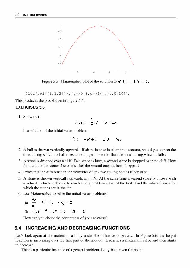
68 FALLING BODIES
2 4 6 8
20
40
60
80
100
Figure 5.5: Mathematica plot of the solution to � � � � � � � � � � � �
Plot[sol[[1,1,2]]/.{g->9.8,u->44},{t,0,10}].
This produces the plot shown in Figure 5.5.
EXERCISES 5.3
1. Show that
� � � � �
�� � � � � � � #
is a solution of the initial value problem
� � � � � � � � ' � � * � � # �
2. A ball is thrown vertically upwards. If air resistance is taken into account, would you expect thetime during which the ball rises to be longer or shorter than the time during which it falls?
3. A stone is dropped over a cliff. Two seconds later, a second stone is dropped over the cliff. Howfar apart are the stones 2 seconds after the second one has been dropped?
4. Prove that the difference in the velocities of any two falling bodies is constant.
5. A stone is thrown vertically upwards at 4 m/s. At the same time a second stone is thrown witha velocity which enables it to reach a height of twice that of the first. Find the ratio of times forwhich the stones are in the air.
6. Use Mathematica to solve the initial value problems:
(a). /
. �� � � � � ' / � * � 2
(b) � � � � � � 3 � � � � � 2 ' � � * � *
How can you check the correctness of your answers?
5.4 INCREASING AND DECREASING FUNCTIONSLet’s look again at the motion of a body under the influence of gravity. In Figure 5.6, the heightfunction is increasing over the first part of the motion. It reaches a maximum value and then startsto decrease.
This is a particular instance of a general problem. Let 6 be a given function:

INCREASING AND DECREASING FUNCTIONS 69
� � � �
� �
� �
� �
� �
� �
�
�
Figure 5.6: The variation of height with time
� Find the portion of its domain where is increasing.
� Find the portion of its domain where is decreasing.
� Find a number � in the domain of for which � � � achieves a maximum or minimum value.
This type of problem occurs more frequently than one might expect. Here are two instances:
1. The amount of carbon dioxide in the atmosphere is increasing as a result of industrial emis-sions. This has given rise to the well-known greenhouse effect, which may have serious cli-matic consequences. The amount of carbon dioxide in the atmosphere is a function of time andis influenced by many factors, including legislation to reduce emissions. Current thinking isthat the total amount of atmospheric carbon dioxide should be limited to no more than twice thepre-industrial levels. To ensure that this happens, it is necessary to be able to determine the ef-fect factors such as restrictions on emission rates and reafforestation will have on the maximumvalue of carbon dioxide in the atmosphere.
2. World population is expected to peak sometime around the middle of the 21st century and there-after to decline. A good knowledge of the population curve is needed for planning purposes.
Let us clarify the precise meaning of increasing and decreasing functions. Let � be an interval inthe domain of a function .
� The function is said to be increasing on � if for any two points � � and � � in � with � � � � � ,we have � � � � � � � � � .
� The function is said to be decreasing on � if for any two points � � and � � in � with � � � � � ,we have � � � � � � � � � .
If we look at the graph in Figure 5.6, it is clear that the slope of the tangent is positive when isincreasing. This suggests (but does not prove) that � � � � will be positive for all � � if is increasingon � . Similarly, we expect � � � � to be negative for all � � if is decreasing on � . These facts canbe proved and we shall assume them to be true. They are summarised in the next theorem.

70 FALLING BODIES
THEOREM 5.2 Increasing and decreasing functionsLet � be differentiable on an interval � � � � .
� If � � � � � for all � in � � � � , then � is increasing on � � � � .
� If � � � � � for all � in � � � � , then � is decreasing on � � � � .
EXAMPLE 5.4Determine the intervals on which the function � � � � � � � � � ! " $ � is
(a) increasing
(b) decreasing.
Solution. We find that
� � � � & � ! � ( * � " $� & � � � ( � � � & 1
From this we see that � � � � � if � � ( or � � & and � � � � � if ( � � � & . Consequently, � isdecreasing if ( � � � & and increasing if � � ( or � � & . The graph of � is plotted in Figure 5.7.
( * & 9
(
*
&
9
:
;
Figure 5.7: The graph of � � � � � � � � � ! " $ � .
5.5 EXTREME VALUESLet us now turn to the problem of finding points where a function � takes on extreme values. We shallassume that all our functions are defined on an open interval or on the union of open intervals. Webegin with a definition.
A function � is said to have a local maximum at � < in its domain if � � � < > � � � for all �sufficiently close to � < . It is said to have a local minimum at � < in its domain if � � � < @ � � � forall � sufficiently close to � < .
A local maximum or local minimum value of a function is often referred to as a local extremevalue of the function. If � � � < is a local extreme value of � , the point � � � � � � < is called a turning

EXTREME VALUES 71
�
�� �� �
� � � � �
Figure 5.8: Local maxima and minima
point of the graph of . The function shown in Figure 5.8 has a local maximum at � � and a localminimum at � � .
The word local is used here to indicate that we are only considering function values close to apoint � � in the domain of the function. In contrast to local extreme values, we can also considerglobal or absolute maxima and minima.
A function is said to have a global maximum at � � in its domain if � � � � � � � � for all � in thedomain of . It is said to have a global minimum at � � in its domain if � � � � � � � � for all � inthe domain of .
�
�� �� �
� � � � � �
Figure 5.9: A function which is not differentiable at its local extrema
In Figure 5.8, does not have a global extreme value at either � � or � � . Figure 5.8 suggests that forsmooth curves the tangent is horizontal at a point � � where has a local extreme value, in which case
� � � � � � " . However, if the curve is not smooth, then there may be no derivative at a point where thefunction has a local maximum or minimum. This is illustrated in Figure 5.9, where the function � haslocal extreme values at � � and � � , but is not differentiable at these points.
There is a theorem which formalises the above observations. We state it without proof.
THEOREM 5.3 Local extreme valuesLet be a function whose domain is an open interval or union of open intervals. If has a localextreme value at a point � � in its domain, then either � � � � � � " or � � � � � does not exist.
A stationary point of a function is a point � � for which � � � � � � " . Thus local maxima andminima of smooth functions are stationary points. There are, however, other possibilities. A stationarypoint which is neither a local maximum nor a local minimum is called a horizontal point of inflexion .In Figure 5.10, both graphs have a horizontal point of inflexion at � � .

72 FALLING BODIES
� � � � ��
� �
Figure 5.10: Horizontal points of inflexion
To determine whether a stationary point is a local maximum, a local minimum or a horizontalpoint of inflexion, we examine the sign of the derivative on either side of the stationary point. This isthe first derivative test.
THEOREM 5.4 The first derivative test for maxima and minimaLet � be a function which has a stationary point at � � in its domain.
� If the sign of � � � changes from positive to negative as � passes through � � , then � has alocal maximum value at � � .
� If the sign of � � � changes from negative to positive as � passes through � � , then � has alocal minimum value at � � .
� If the sign of � � � does not change as � passes through � � , then � has a horizontal point ofinflexion at � � .
We shall use the notation � � to denote a number close to, but less than � , while � � will denote anumber close to, but larger than � .
EXAMPLE 5.5Determine the nature of the stationary points of
� � � � � � � � � � � �
Solution. We have � � � � " � # � � , so that � � � � % when � � ' ( ) . Since � ( ) � � + % and
� ( ) � � . % , we see that the sign of � � � changes from negative to positive as � passes through( ) . Consequently, � has a local minimum at ( ) . Similarly, there is a local maximum at � ( ) .
5.5.1 Concavity
Consider Figure 5.11, which shows the graph of a function � . On the interval 1 2 4 � , the graph,roughly speaking, curves up, while on the interval 4 2 � � , it curves down. The technical terms for thisbehaviour are concave up and concave down . In the definition below, we can make these terms preciseby noticing that on the interval 1 2 4 � , the function � is increasing, while on 4 2 � � , the function � isdecreasing. (Why?)

EXTREME VALUES 73
�
�� � �
� � � �
concave down
concave up
Figure 5.11: Concavity on an interval
Let be a function which is differentiable on an open interval � . The graph of is said to be concaveup on � if � is increasing on � . The graph of is said to be concave down on � if � is decreasingon � .
Suppose that � is differentiable on an open interval � . It follows that if the graph of is concaveup on � , then � � � � � � for all � � . If the graph of is concave down on � , then � � � � � �for all � � . A point ! where the concavity of the graph of changes sign is called a point ofinflexion , in which case � � � ! � � � . Note carefully that the converse of this result is not true. Theresult � � � ! � � � does not imply that there is a point of inflexion at ! . An example of a point ofinflexion occurs in Figure 5.11, where the graph of has a point of inflexion at � � ) � � � � .
EXERCISES 5.5
In Exercises 1–4, find the intervals on which increases and the intervals on which decreases.
1. � � � / 0 2 5 7 2. � � � / � 9 5 �3. � � � < 5 0 2 � 4. � � � > 7 5 @ >
In Exercises 5–8, find the stationary points of and the local extreme values.
5. � � � B < 0 C 6. � � � D 0 9 C <
7. � � � > < 0 9 F > 8. � � � 9 5 9 0
9. Find the extreme values of the function � � � < 0 B 5 9 ) � M M 2 O10. A rectangle has a perimeter of 7 B cm. Find the dimensions of the sides that will give the
largest area.
11. A beam with a rectangular cross section is to be cut from a circular log of radius 9 P cm. Thestrength of such a beam is proportional to � Q < , where � is its breadth and Q its width. Find thedimensions of the strongest beam that can be obtained.
12. An open gutter is to be made from sheet metal of width 7 7 cm by folding up identical strips oneach side, so that they are at right angles to the base. Determine the dimensions of the gutter thatwill have the greatest carrying capacity.

This page intentionally left blank

CHAPTER 6SERIES AND THE EXPONENTIAL FUNCTION
In Chapter 5, we solved the problem of bodies moving freely under the influence of gravity by consid-ering some experimental results, using these results to obtain a differential equation and then solvingthis equation to find the required function that expresses height in terms of time. This same procedurewill be used to deal with the second problem, but we shall require a new way of defining functions inorder to find the solution.
6.1 THE AIR PRESSURE PROBLEM
The measurement of air pressure is not a simple matter, because air pressure at any given heightvaries with time. Indeed, this variation is one of the main factors determining weather conditions.Technically, air pressure is a function of two variables, the height � and the time � . We shall notbe considering functions with two independent variables in this book and so we shall make somesimplifying assumptions.
The SI unit of pressure is the pascal (Pa), which is the pressure exerted by a cylinder of crosssection 1 m � and height sufficient to give it a mass of 1 kg. However, for historical reasons air pressureis measured in hectopascals (hPa), where one hectopascal is 100 pascals. At sea level, the air pressurevaries between 980 and 1030 hectopascals, depending on the weather conditions, but the averagevalue is 1013 hectopascals. Meteorologists usually express the pressure in millibars (mb), where 1 mbis equivalent to 1 hPa.
Instead of bringing the time variation into our considerations, we shall look at the average pressureat each height. By using this average we obtain the values given in Table 6.1. In this table, we denotethe pressure by � and the height by � . Height is the independent variable and is given in steps of1000 m up to 10 000 m, which is about the maximum height of a commercial airliner.
� 0 1000 2000 3000 4000 5000 6000 7000 8000 9000 10 000
� 1013 899 795 701 616 540 472 411 356 307 264
Table 6.1: Average air pressure
Plotting � against � gives the curve shown in Figure 6.1.
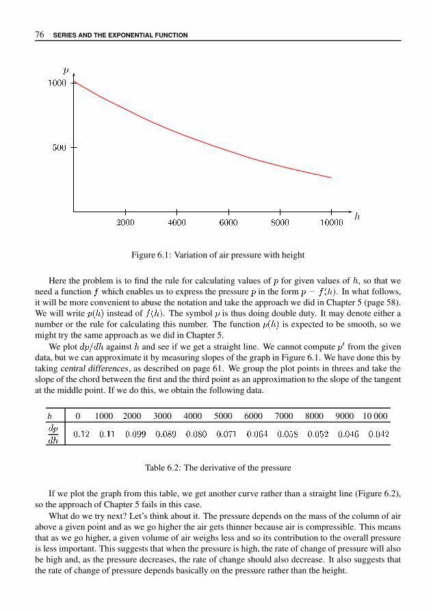
76 SERIES AND THE EXPONENTIAL FUNCTION
� � � � � � � � � � � � � � � � � � � �
� � �
� � �
�
�
Figure 6.1: Variation of air pressure with height
Here the problem is to find the rule for calculating values of � for given values of , so that weneed a function � which enables us to express the pressure � in the form � � � � � . In what follows,it will be more convenient to abuse the notation and take the approach we did in Chapter 5 (page 58).We will write � � � instead of � � � . The symbol � is thus doing double duty. It may denote either anumber or the rule for calculating this number. The function � � � is expected to be smooth, so wemight try the same approach as we did in Chapter 5.
We plot � � � � against and see if we get a straight line. We cannot compute � � from the givendata, but we can approximate it by measuring slopes of the graph in Figure 6.1. We have done this bytaking central differences, as described on page 61. We group the plot points in threes and take theslope of the chord between the first and the third point as an approximation to the slope of the tangentat the middle point. If we do this, we obtain the following data.
0 1000 2000 3000 4000 5000 6000 7000 8000 9000 10 000� �
� � � " � � � " � � " � & & � � " � � & � � " � � � � � " � ( � � " � � � � � " � � � � � " � � � � � " � � � � � " � � �
Table 6.2: The derivative of the pressure
If we plot the graph from this table, we get another curve rather than a straight line (Figure 6.2),so the approach of Chapter 5 fails in this case.
What do we try next? Let’s think about it. The pressure depends on the mass of the column of airabove a given point and as we go higher the air gets thinner because air is compressible. This meansthat as we go higher, a given volume of air weighs less and so its contribution to the overall pressureis less important. This suggests that when the pressure is high, the rate of change of pressure will alsobe high and, as the pressure decreases, the rate of change should also decrease. It also suggests thatthe rate of change of pressure depends basically on the pressure rather than the height.

THE AIR PRESSURE PROBLEM 77
� � � � � � � � � � � � � � � � � � � ��
� � �
� � � �
� � � �
� � � � �
�
� �� � � � � � � � �
Figure 6.2: Variation of the derivative of the air pressure with height
Given this argument, we try plotting � � against � and see what happens. We don’t know in advanceif this will achieve anything, but it illustrates the way in which we must use all our physical intuitionabout a given situation in trying to produce a workable mathematical model of it. In this case we doindeed get a straight line (Figure 6.3) to within a small amount of error.
� � � � � � � � � � � � � � ��
� � �
� � � �
� � � �
� � � � �
�
�����������
Figure 6.3: Variation of the derivative of the pressure with pressure
The equation of this line can be obtained and this equation, together with the initial value � � � � � � � , gives us the initial value problem
� � � � � � � � � � � � � � � � � � � � � � � # � � � � � � � � (6.1)
It is this initial value problem that has to be solved for the pressure as a function of height. It is morecomplicated than those we encountered in Chapter 5 for two reasons. First, the constants are lessfriendly than the previous cases. More importantly, the function � as well as its derivative appearsin the equation. This seemingly minor matter actually complicates the solution considerably. Ratherthan attack equation (6.1) directly, we consider a simpler form. This is often a useful procedure in

78 SERIES AND THE EXPONENTIAL FUNCTION
difficult problems. Examine an easier version of the problem first in order to gain the necessary insightbefore attempting the more difficult problem. Equation (6.1) has the form
� � � � � � � � � � � � � � � � � �
where � , � and � are constants. We shall consider the special case � � , � � and � � . That is, weconsider the initial value problem
� � � � � � � � � � � � � � � �
We now have a problem which is purely mathematical, namely the problem of finding � from thisequation. In words, this problem is to find a function which is equal to its own derivative. This is atypical instance of the way mathematical and scientific ideas develop in tandem. A physical problemgives rise to a mathematical problem and subsequent investigation of the mathematical problem mayshed new light on the physical problem. We take a general approach and put # � & � and, if isequal to its own derivative, then
( ( &
� � � � � � (6.2)
To solve this problem we need to find as a function of & . There is more than one way of doing thisand we shall consider two methods in this book, one in this chapter and another in Chapter 10.
We begin by trying the approach we developed in Chapter 5, where we solved differential equa-tions by using polynomial functions as trial solutions. Although this will not work here for reasonswhich will soon become clear, it is still useful to see what happens if we attempt to use polynomialsas trial solutions. We find out why they don’t work and what we have to do to actually get the solutionwe are seeking. The methods developed will prove to be useful in later problems.
Take a trial solution � & � , where � and � are constants. If we substitute this into the firstequation of (6.2), the left hand side becomes
( ( &
�
while the right hand side is � & � �
We then have � � & � and so equating coefficients gives � � and � � . Thus � & � � forall values of & . This is a solution of the differential equation, but does not satisfy the initial condition � � � � . If we try a higher degree polynomial, a similar problem arises. Suppose, for example, wetry � & 6 � & 9 � & ( . Then the left hand side of the first equation in (6.2) becomes
( ( &
; � & 9 < � & �
while the right hand side is � & 6 � & 9 � & ( �
We then have; � & 9 < � & � � & 6 � & 9 � & ( � (6.3)
Once again, there is a discrepancy between the degrees of the terms on the two sides of the equation—the left hand side has degree 2, while the right hand side has degree 3. If we equate coefficients
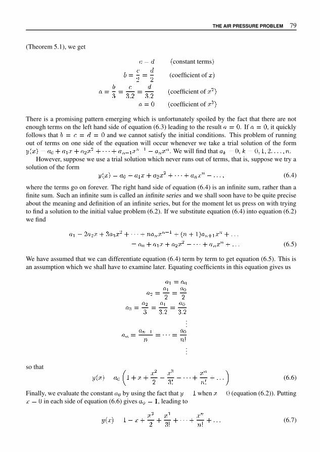
THE AIR PRESSURE PROBLEM 79
(Theorem 5.1), we get
� � � � constant terms �� � � � � (coefficient of �
� � �� � �� � � �� � � coefficient of � �� � � � coefficient of � �
There is a promising pattern emerging which is unfortunately spoiled by the fact that there are notenough terms on the left hand side of equation (6.3) leading to the result � � � . If � � � , it quicklyfollows that � � � � � � � and we cannot satisfy the initial conditions. This problem of runningout of terms on one side of the equation will occur whenever we take a trial solution of the form � � � � % ' � ) ' � � � ' * * * ' � . / ) . / ) ' � . . . We will find that � � � � , 1 � � 2 3 2 2 � � � 2 9 .
However, suppose we use a trial solution which never runs out of terms, that is, suppose we try asolution of the form � � � � % ' � ) ' � � � ' * * * ' � . . ' � � � 2 (6.4)
where the terms go on forever. The right hand side of equation (6.4) is an infinite sum, rather than afinite sum. Such an infinite sum is called an infinite series and we shall soon have to be quite preciseabout the meaning and definition of an infinite series, but for the moment let us press on with tryingto find a solution to the initial value problem (6.2). If we substitute equation (6.4) into equation (6.2)we find
� ) ' � � ' � � � � ' * * * ' 9 � . . / ) ' � 9 ' 3 � � . A ) . ' � � �� � % ' � ) ' � � � ' * * * ' � . . ' � � � (6.5)
We have assumed that we can differentiate equation (6.4) term by term to get equation (6.5). This isan assumption which we shall have to examine later. Equating coefficients in this equation gives us
� ) � � %� � � � ) � � %� � � � �� � � )� � � � %� �
...� . � � . / )9 � * * * � � %9 D
...
so that
� � � � % F 3 ' ' � ' �� D ' * * * ' .9 D ' � � � G (6.6)
Finally, we evaluate the constant � % by using the fact that � 3 when � � (equation (6.2)). Putting � � in each side of equation (6.6) gives � % � 3 , leading to
� � � 3 ' ' � ' �� D ' * * * ' .9 D ' � � � (6.7)

80 SERIES AND THE EXPONENTIAL FUNCTION
At this stage it is not clear that we can get any useful information out of equation (6.7). How canwe operate sensibly with an infinite number of terms? We certainly cannot add up an infinite numberof terms, because the additions go on forever. In part, the answer lies in the fact that in any practicalcalculation we only want accuracy to a certain number of decimal places. Notice that in equation (6.7),the denominators of the terms become larger as we move to the right, so that for a fixed value of � , wewould expect that eventually successive terms will become smaller and smaller. What we hope is thatthey become so small that we can ignore all terms after a certain number and still attain the accuracywe want. In the case of equation (6.7) this is indeed what happens. We can illustrate (but not prove)this in the following table. We have used Mathematica to calculate the finite sum
� � � � � � � �
�
� �� �
� � � � �
� �
for three values of � and various increasing values of � .
� � � � $ � � � � $ � $ � �
� � 1 2 2.70823 2.71828 2.71828 2.71828 2.71828
� $ 1 6 65.375 143.689 148.38 148.413 148.413
� � 1 11 644.333 10086.6 20188.2 22026.5 22026.5
Table 6.3: Partial sums � � � �
� � � � �
� �
� �for various values of � and �
Notice how, for a given � , the terms all appear to approach a fixed value as � becomes progres-sively larger. The technical term for this phenomenon is known as convergence. A table such as thisis not conclusive, but it does suggest that if we fix a value of � , then by taking enough terms of theseries (6.7) we can calculate � � � � to any accuracy we want. In the next section, we will considerinfinite series in more detail, with a view to justifying these assertions.
The calculations we have carried out here are all exploratory and suggestive of methods whichmight be used to find a solution of the initial value problem � , � � � � � � � , � � � � . Our task now isto investigate how to make them precise. We have to answer questions such as:
1 How do we add up an infinite sum?
1 Can we differentiate an infinite sum of functions in the same way as a finite sum?
1 Is there a function, defined as an infinite sum, which is a solution of the differential equation?
EXERCISES 6.1
1. The following table gives the density 2 of the atmosphere at a height 3 , for different values of3 . The density is given as a fraction of the mean sea level density, while the height is givenin kilometres. Based on this data, determine a differential equation relating the height and thedensity.
2 0.5 0.25 0.125 0.0625 0.0312 0.0156 0.0078 0.0039 0.0019
3 5.28 10.56 15.84 21.12 26.40 31.68 36.96 42.24 47.52

INFINITE SERIES 81
6.2 INFINITE SERIESWe begin with a provisional definition:
Provisional definition 6.1 A series is an infinite sum of numbers. The numbers which appear in thesum are called the terms of the series.
There are two types of notation for series. The first is to write down the first few terms of the seriesand use dots to indicate that the sum does not terminate. This is the way we have written series in the
discussion above. The second is to use summation notation. The symbol
��� � �
� � is used to denote the
finite sum � � � � � � � � � , while �
� � �� � is used to denote the infinite sum � � � � � � � � � . We
may replace � � by a formula involving � in both the above cases.
EXAMPLE 6.1Some particular series are:
� � ��
��
��
��
�� or
�� � �
�� � � �
� � � � � � � � � or
�� � �
�
� � ��
��
��
��
�� or
�� � �
��
� � !�
��
��
!�
�� or
�� � �
" ! � & � ' ��
(
It is somewhat misleading to say that a series is an infinite sum, because there is no way to add up aninfinite number of terms in the same way that we can do for a finite sum. To say what is meant bythe sum of a series requires the theory of sequences which we discussed in Chapter 2. We recall thefollowing facts on sequences:
� A sequence is an infinite list of numbers. The numbers in the list are called the terms of thesequence.
� A sequence ) � � , is said to be convergent if - . /� 1 � � exists. Otherwise the sequence is said to
be divergent.
It is essential to be clear about the difference between sequences (lists) and series (sums). It shouldbe noted that in everyday usage, sequences are almost always referred to as series. For example, a listof stock market prices is referred to as a series of prices.
There are two sequences associated with every series. The first is the sequence of terms. Forexample, in the series �
� � �� 4 " � � � � & 7 � �
��
��
��
��
� :

82 SERIES AND THE EXPONENTIAL FUNCTION
the sequence of terms is � � �� � �� � �� � � � �The sequence of terms is important in the theory of series, but much more important is the second ofthe two sequences associated with a series. This is the sequence of partial sums.
DEFINITION 6.1 Partial sums:The th partial sum of the series � � � � � is the sum of the first terms of the series. It is denotedby � � and so � � � � � � � � � � � � .
The partial sums of a series form a sequence � � � � � � � � � � � � � � � , and it is this sequence which enablesus to say what we mean by the sum of a series.
DEFINITION 6.2 Sum of a series:Let � � � � � be a series and let � � � " be its sequence of partial sums. The series is said to beconvergent if the sequence � � � " is convergent. If the series is convergent, then # $ % � ' � � is calledthe sum of the series and is denoted by � � � � � . A series which is not convergent is divergent.
It is not usually possible to find a formula for the sum of a convergent series, except in some specialcases.
EXAMPLE 6.2Consider the series �
� � � ) � + � � � � ) � ) � � ) � � � � � (6.8)
The th partial sum of this series is
� � � ��� � � ) � + � � � � ) � ) � � ) � � � � � � ) � + � �
This is a finite geometric series with sum
� � � � 2 ) �� 2 ) �To determine the convergence properties of the infinite series, we look at the sequence of partial sums
� � � " � 5 � 2 ) �� 2 ) 6 �There are two cases to consider:7 If 8 ) 8 ; � , that is, 2 � ; ) ; � , then ) � A C as A F , so that � � A �� 2 ) as A F . Thus
if 8 ) 8 ; � we can write � � ) � ) � � ) � � � � � � �� 2 )for the sum of the series (6.8).7 If 8 ) 8 G � , then � ) � " diverges and so the sequence of partial sums also diverges. This meansthat the series (6.8) diverges if ) G � .
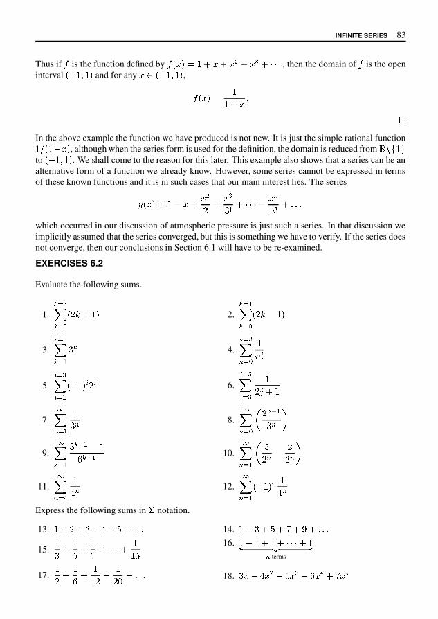
INFINITE SERIES 83
Thus if � is the function defined by � � � � � � � � � � � � � , then the domain of � is the openinterval � � � � � � and for any � � � � � � � � ,
� � � � �� � � !"
In the above example the function we have produced is not new. It is just the simple rational function� $ � � � � � , although when the series form is used for the definition, the domain is reduced from ' ( ) � ,to � � � � � � . We shall come to the reason for this later. This example also shows that a series can be analternative form of a function we already know. However, some series cannot be expressed in termsof these known functions and it is in such cases that our main interest lies. The series
- � � � � � � �1 � �2 4 � � � � 56 4 ! ! !
which occurred in our discussion of atmospheric pressure is just such a series. In that discussion weimplicitly assumed that the series converged, but this is something we have to verify. If the series doesnot converge, then our conclusions in Section 6.1 will have to be re-examined.
EXERCISES 6.2
Evaluate the following sums.
1.� 8 ��� 8 : � 1 < � � 2.
� 8 =�� 8 : � 1 < � � �
3.
� 8 ��� 8 ?
2 � 4.
5 8 ��5 8 :
�6 45.
� 8 ��� 8 ?
� � � � � 1 � 6.
� 8 @�� 8 �
�1 � �7.
B�5 8 ?
�2 5 8.
B�5 8 : C 1 5 D ?2 5 E
9.
B�� 8 ?
2 � G ? � �H � G ? 10.B�
5 8 ?C I1 5 � 12 5 E
11.B�
5 8 =�J 5 12.
B�5 8 ?
� � � � 5 �J 5Express the following sums in � notation.
13. � 1 2 J I ! ! ! 14. � 2 I O P ! ! !15.
�2 �I �O � � � �� I 16. � � � � � � �� � �5 terms
17.�1 �H �� 1 �1 Q ! ! ! 18. 2 � � J � � I � � � H � = O � @

84 SERIES AND THE EXPONENTIAL FUNCTION
Suppose that � � � � � � � � � and � � � � � � � � � . Find the values of the following sums.
19.
��� � �
� � � 20.
��� � �
� � � � � �
21.
��� � �
� � � � � � � � 22.
��� � �
� ��23. Show that
� � � � � � � � � � " � " � " � � �� (24. Sum the series )�
� � �* �+ " � � � �+ " � � - (
25. Verify that �" � " � � � � �" � �" � � (Hence show that )�
� � ��" � " � � � � � (
26. Verify that �� " � � � � " � � � � �" � � � �" � � (Hence evaluate )�
� � ��� " � � � � " � � � (
27. Verify that 1� � " � � � � � " � � � � �� " � � � �� " � � (Hence evaluate )�
� � �1� " 4 � � (
6.3 CONVERGENCE OF SERIES
There are a variety of methods for determining whether a given series converges or not. In Exam-ple 6.2 we computed the sum of a series by computing a sequence of partial sums and then finding thelimit of this sequence of partial sums. Such direct methods are usually not possible except in a fewsimple cases, so that indirect methods are necessary. One of the most useful and important tests forconvergence is the ratio test which we state without proof.

CONVERGENCE OF SERIES 85
THEOREM 6.1 The ratio testLet ��
� � � � � � � � � � � � � � � � � (6.9)
be a given series of non-zero terms. Suppose that the sequence
����� � � ����
� ����� �� ����
� ����� �� � ����
� � � � � � ����� � � �� � ����
�converges to a limit � .
1. If � � � , then the series (6.9) converges.
2. If � � � , then the series (6.9) diverges.
3. If � � � , then no conclusion can be drawn. The series (6.9) may converge or it may diverge.
Let us apply this test to the function defined by
� " $ � � � " � " ' ) � " �+ ) � � � � . (6.10)
For a particular value of " , the / th term is " � 1 � 2 / 5 � $ ) and using the ratio test we have
8 9 :� < � ����" � 2 / )" � 1 � 2 / 5 � $ ) ����
� 8 9 :� < � ���" / ���� @ " @ 8 9 :� < � �/� A .
Since this holds for every value of " , it follows that the series converges for every " and so thedomain of � is B . For any " D B , if we take enough terms of the series, we can compute � " $ toany required accuracy. This raises an immediate question. How do we determine when enough termshave been taken? Let us put this another way. We want to determine F so that
� � " � " ' � " �+ ) � � � � � " GF )gives the sum of the series
� " $ � � � " � " ' � " �+ ) � � � � � " GF ) � . . .to within the required accuracy. Let us write
� " $ � � � " � " ' � " �+ ) � � � � � " GF ) � � � �� J G � " GF ) � " G � � F � � $ ) � � � �� J G � N G .
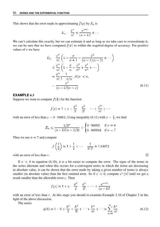
86 SERIES AND THE EXPONENTIAL FUNCTION
This shows that the error made in approximating � � � � by � is
� � � � � � � � �� � � � � � � � � �We can’t calculate this exactly, but we can estimate it and as long as we take care to overestimate it,we can be sure that we have computed � � � � to within the required degree of accuracy. For positivevalues of � we have � � � � � � � � �� � � � � �� � � � � � � � # � � � � � %& � � � � � � �� � � �� � � � (� ( � � � � %� � � � �� * � , � - if . � . 0 � ,
� � � � * � � � � � * � � (6.11)
EXAMPLE 6.3Suppose we want to compute � � �� � for the function
� � � � � � � � � � �# � � (8 � � � � � � � � � � � � �with an error of less than : � = � = = = = � @ Using inequality (6.11) with � � �� , we find
� & � , # � � * � � � � � * � , # � 0 B = � = = = = 8 if � � D= � = = = = = # if � � GThus we use � � G and compute
� � �# % � � � �# � � � � � �# I G � @� � @ D L M G #with an error of less than : . N
If � 0 = in equation (6.10), it is a bit easier to compute the error. The signs of the terms inthe series alternate and when this occurs for a convergent series in which the terms are decreasingin absolute value, it can be shown that the error made by taking a given number of terms is alwayssmaller (in absolute value) than the first omitted term. So if � 0 = , compute � , � � until we get aresult smaller than the allowable error : . Then� � � � � � � � � � �# � � (8 � � � � � � � R �� � * � � �with an error of less than : . At this stage you should re-examine Example 2.16 of Chapter 2 in thelight of the above discussion.
The series S � U � � � � U � U �# � U (8 � � � � � � U � � � � � � � X� Y Z U � � (6.12)

CONVERGENCE OF SERIES 87
� � �� �� �
����
�
�
� � � � �
Figure 6.4: The exponential function
has been shown to converge for each value of . We now reach a very important definition.
DEFINITION 6.3 The exponential function:The exponential function � � � � � � is defined by
� � � � � � � � � � � � �� � � �
� � � � � #$ � � �
'�# ( )
� #$ � *
For reasons which will become clear later on, we often write + - for � � � � � � , where + is a constantwhose value is + � � * 1 � 3 � 3 * * * The domain of the exponential function is 6 and by calculating� � � � � � for various values of � , we can plot its graph, as in Figure 6.4. The value of � � � � � � is easilyseen to be 1.
We were led to the exponential function because of our interest in the initial value problem 8 : � � � �8 � � � , 8 � � � � � . To show that � � � � � � satisfies this initial value problem is, in principle, a simplematter. We have to show that
@@ � � � � � � � � � � � � � � C � � � � � � � � *
The first of these equations is the one that will cause concern. In order to evaluate
@@ � � � � � � � C
we have to know how to differentiate the series which defines the exponential function. More gen-erally, we would like to know how to differentiate any series, assuming that such a series is differ-entiable. In going from equation (6.4) to equation (6.5), we assumed that we could differentiate theseries term by term. This is indeed true in this case, but is not true for series in general. We need tobe precise about what we can and cannot do when differentiating series. This will be discussed in thenext section. We conclude this section with some additional examples on the use of the ratio test.
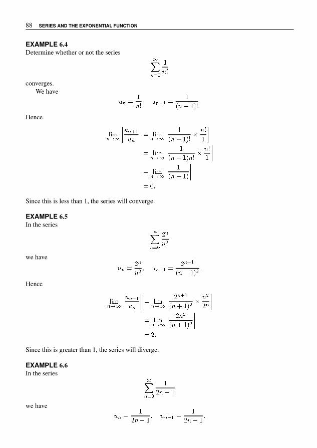
88 SERIES AND THE EXPONENTIAL FUNCTION
EXAMPLE 6.4Determine whether or not the series ��
� � ��
� �converges.
We have
� � �� � � � � � �
� � � � � � �Hence
� � �� � � !!!!
� � � � !!!!� � � �� � � !!!!
�� � � � � � $ � �
� !!!!� � � �� � � !!!!
�� � � � � � � $ � �
� ! !!!� � � �� � � !!!!
�� � � � � !!!!� ' �
Since this is less than 1, the series will converge.
EXAMPLE 6.5In the series ��
� � �) �
� *we have
� � ) �� * � � � � ) � � �
� � � � � * �Hence
� � �� � � !!!!
� � � � !!!!� � � �� � � !!!!
) � � �� � � � � * $ � *
) � !!!!� � � �� � � !!!!
) � *� � � � � * !!!!� ) �
Since this is greater than 1, the series will diverge.
EXAMPLE 6.6In the series ��
� � ��
) � 0 �we have
� � �) � 0 � � � � � �
) � � � �
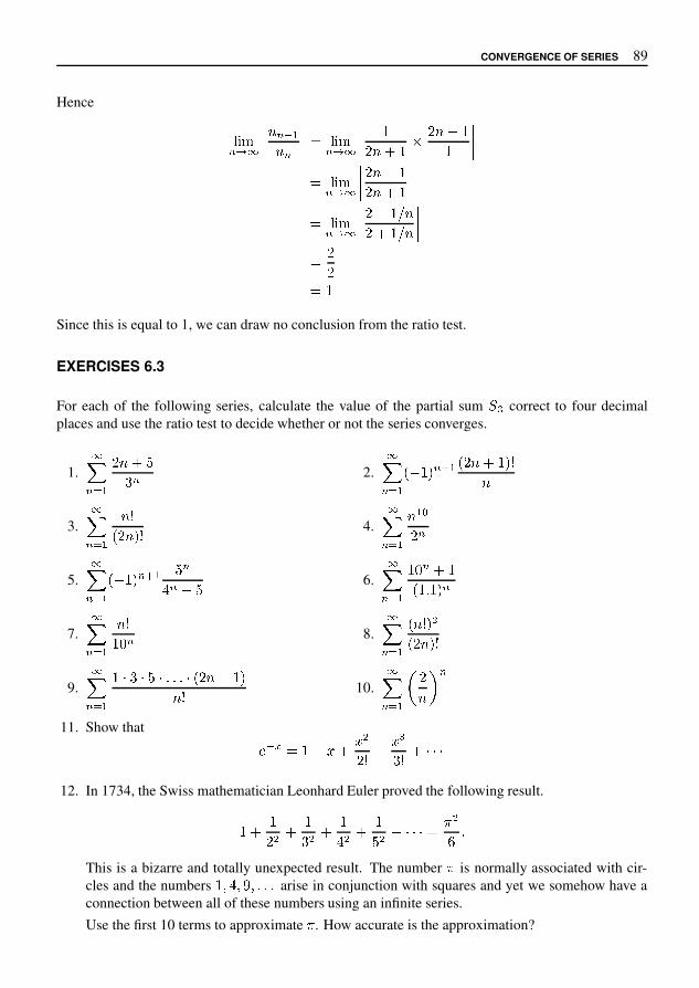
CONVERGENCE OF SERIES 89
Hence
� � �� � � � � �
� � � �� � � �� � � � � � � � �� � � � �� � �
� � � �� � � � � � � �� � � � � � � �� � � � � � � �� �
Since this is equal to 1, we can draw no conclusion from the ratio test.
EXERCISES 6.3
For each of the following series, calculate the value of the partial sum $ % correct to four decimalplaces and use the ratio test to decide whether or not the series converges.
1.
��
� & �� � � () � 2.
��
� & �* � � - � � * � � � � - 0�
3.
��
� & �� 0* � � - 0 4.
��
� & �� � 3
� �5.
��
� & �* � � - � � ( �
4 � � ( 6.��
� & �� 6 � � �* � 7 � - �
7.��
� & �� 0� 6 � 8.
��
� & �* � 0 - 9* � � - 0
9.
��
� & �� ; ) ; ( ; 7 7 7 ; * � � � � -� 0 10.
��
� & �> �� ?
�
11. Show that
@ A B � � � E � E 9� 0 � E %) 0 � ; ; ;12. In 1734, the Swiss mathematician Leonhard Euler proved the following result.
� � �� 9 � �) 9 � �4 9 � �( 9 � ; ; ; � K 9L 7This is a bizarre and totally unexpected result. The number K is normally associated with cir-cles and the numbers � M 4 M Q M 7 7 7 arise in conjunction with squares and yet we somehow have aconnection between all of these numbers using an infinite series.
Use the first 10 terms to approximate K . How accurate is the approximation?

90 SERIES AND THE EXPONENTIAL FUNCTION
13. Use the first 5 terms of the series expansion of � � � � � � to approximate � � � � � � � . Calculate themaximum possible error in the approximation.
14. Suppose that the first 6 terms of the series
� � � � �� � � � �
� � � � � � � � �� � � � � �
are used to approximate ! � � . What is the value of the approximation? How accurate is theapproximation?
6.4 RADIUS OF CONVERGENCEFrom now on we shall focus on series of functions, that is, each term in the series is a function, ratherthan a number. In particular, we shall consider power series, which are of the form
"� # ! $ � % $ ! � $ ) � � $ � � � � $ � � � � � � � � $ � � � � � +
where $ , , % + � + � + are all constants.Consider a function 2 defined by a power series:
2 � � � % $ ! � $ ) � � $ � � � � $ � � � � � � � � $ � � � � � To determine where this series converges we apply the ratio test, assuming that all the coefficients arenon-zero.
5 6 7� 8 " ::::$ � < ) � � < )
$ � � � ::::% 5 6 7� 8 " ::::
$ � < ) �$ � ::::% ? � ? 5 6 7� 8 " ::::
$ � < )$ � ::::
There are three cases to distinguish.B Suppose that there is a positive number such that
5 6 7� 8 " ::::$ � < )$ � ::::
% If we choose � so that ? � ? C F , then
5 6 7� 8 " ::::$ � < ) � � < )
$ � � � ::::% ? � ? C +
and so the series will converge by the ratio test. The number F is called the radius of con-vergence and is usually denoted by the symbol H . The series converges for all ? � ? C H anddiverges for all � such that ? � ? J H . The interval � M H + H � is called the interval of convergence.
B If
5 6 7� 8 " ::::$ � < )$ � ::::
% � +then the series converges for every value of � and we say that the radius of convergence isinfinite. We write H % R . The interval of convergence is � M R + R � .

RADIUS OF CONVERGENCE 91
� If
� � �� � � � � �� �
� � �then the series converges only for � � � . We say that the radius of convergence is zero. Thereis no interval of convergence.
From this, we conclude that every power series has a radius of convergence and the series convergesin a symmetric interval about the origin. There are three further points we should note:
� The series may or may not converge at the end points of the interval, that is, at the points� � � � . We shall not investigate this issue in any detail.
� It may be that � � � � � � � � � ! � � does not exist. The series will still have a radius of conver-gence, but it will be more difficult to determine. This will not occur in any of our examples.
� We shall meet cases of power series where only even or only odd powers of � occur. In thiscase some of the constants � � will be zero and the above arguments will need to be modified.This does not cause any problem and we shall deal with such cases as they arise. Such seriesstill have a radius of convergence and there will usually be no difficulty in determining it.
EXAMPLE 6.7We have already discussed the series
$ & � & � ) & � * & + + +in Example 6.2 and the results we got there show that its interval of convergence is - / $ � $ 2 . Let usderive the same result by applying the ratio test to the series. We have
� � �� � � � � �
� � � � � �� � � � � 6 $ �
as long as � is in the interval - / $ � $ 2 .We also know that
$ & � & � ) & � * & + + + � $$ / � 9
Since we cannot put � � $ in the right hand side, the series cannot converge for this point. There is noproblem with any � 6 � and we might have expected the series to converge for all negative values of� . However, since the interval of convergence of a power series has to be a symmetric interval aboutthe origin, and the series diverges at � � $ , so the interval must be - / $ � $ 2 .
EXAMPLE 6.8Determine the radius of convergence of the series
�� < =
� ) �> � � $ & � )
> & � @> ) & � B
> * & 9 9 9

92 SERIES AND THE EXPONENTIAL FUNCTION
Here
� � �� � �
� � � � � � �� � �
� � � � � �� � � � � �
� � � � � � �� � �
� �� � � �
as long as � � � � � � , that is, if � � � � � � � � . Hence the radius of convergence is � � .
EXERCISES 6.4
Find the radius of convergence and interval of convergence of each of the following power series.Ignore the problem of convergence at the end points.
1.��
� # �� �
$ & � � 2.��
� # �' � � + � $ -
. � � �
3.
��� # �
� � � � �4.
��� # �
' � � + � � � �/ � �
5.
��� # �
0 $ � � � 6.
��� # �
' � � + � � � � �' � $ 4 � + &
7.
��� # �
� � � �. � ' � $ 4 � + 8.
��� # �
$ & � �
9.
��� # �
' � � + �$ & ' $ 4 � + & 9
�� : � � � 10.
��� # �
� < / < > < @ @ @ < ' . $ � � +' . $ + & � - �
Find the interval of convergence of each of the series in Exercises 11–15. Ignore the problem ofconvergence at the end points.
11.
��� # �
' � � + �$ ' � � � + � 12.
��� # �
. $ �0 � ' � 4 � + �
13.
��� # �
' � 4 � + � �� � $ & 14.
��� # �
' � � + � $. $ 4 � ' � 4 � + � �
15.
��� # �
' � $ � � + . �$ & ' � � . + �
DIFFERENTIATION OF POWER SERIES 93
16. Verify that�
� ��
�� � � � �
�
� � � � � ��
Hence, using the result of question 7 in Exercises 6.2, show that
��
� � �
�� �
� � ��
� � �
�� � � � � �
�
We could compute ��
� � �
�� �
to a given accuracy by using either one side or the other of the equation above. Which expressionwould be more efficient for doing this? Explain your reasons.[This is a technique known as improving the convergence of a series. It has obvious practicalimplications.]
6.5 DIFFERENTIATION OF POWER SERIES
We now present a very important result. It tells us how to differentiate a function defined by a powerseries inside its radius of convergence. The result is proved using differentiation by first principles,but the proof is rather difficult and we shall not present it here. The result is as follows.
THEOREM 6.2 The derivative of a power seriesLet � be a function defined by a power series
� � � � � � � � � � ��
� � � � ! ! ! � � � � ! ! !
and let the radius of convergence be # % & . Then the function � is differentiable everywhere in theinterval � ( # + # � and
� . � � � � � � 0 ��
� 2 � � � ! ! ! 5 � � � � 8 � ! ! ! �
The radius of convergence of the series for the derivative is also # .
This result is not surprising, but it does tell us something very new. We know from Theorem 4.2 thatthe derivative of a finite sum of functions is the sum of the derivatives and the result above tells usthat the same is true for an infinite sum of positive integer power functions. However, it is not truefor all infinite sums of functions. In fact, an infinite sum of differentiable functions may not even becontinuous and therefore certainly not differentiable. A simple example is the series
� �� � �
� �
� � � � � �
� �� � � � �
! ! !
This is a geometric series and for any � <� & , its sum is 1. If � � & , then the sum is 0. Hence thefunction is not continuous at � � & , and so is not differentiable there. It is, of course, not a powerseries.

94 SERIES AND THE EXPONENTIAL FUNCTION
EXAMPLE 6.9As a first example of the use of Theorem 6.2, consider the exponential function
� � � � � � � � � �� �
� ��
� �� �
� � � �
The above result tells us that
� � � � � � � � � � �� �
� ��
� � �� �
� � � � �! � # % &
! �� ( ( (
� � � �� �
� ��
� �� �
� � � �
� � � � � � � ( *
The above example exhibits a remarkable property of the exponential function, namely that the func-tion and its derivative are identical. The only functions which have this property are the functions
+ � � � � , where + . 0 .
THEOREM 6.3 The derivative of the exponential functionFor all � . 0 , we have
22 �
� � � � � � � � � � � � � (
We can now see that the exponential function is a solution of the initial value problem 4 � � � � � 4 � � � ,4 � � � � � . We still have not solved the equation
: � � ; � � < � ( � � � � ? : � ; � < � ( � � C : � � � � � �
of Section 6.1, but we are making progress.
EXERCISES 6.5
1. Find the radius of convergence of the series
F � � � � � � � � � � � � � � K � L � M � N � O � P � R � S � ( ( (
What is the derivative of F ? Justify your answer.
2. Let
F � � � � T U � T & � � T�
� � � T � � � � � � � �W� X U
T � C
for < Y Z � Z Y . Explain why the conclusion of Theorem 6.2 can be written in the form
22 �
W� X UT �
��
W� X &
+ T � % & C
for < Y Z � Z Y . In particular, explain why the index of summation + starts from 0 in the firstsum and from 1 in the second sum.

DIFFERENTIATION OF POWER SERIES 95
3. Explain why the functions
� � � � � �� �
� ��
� �� �
�� �
� �� � � �
and
� � � � � �� !
" ��
� #$ �
�� &
' �� � � �
are differentiable for all � ) * . What are the derivatives of � and � ?
4. Show that the functions � and � of the previous exercise both satisfy the differential equation+ , , � + . /
5. Explain why the function
� � � � � �� �
��
� ��
�� �
�� � � �
is differentiable for � � 2 � 2 � . Show that � satisfies the differential equation
� , � � � �
� � � !/
6. Show that�
� � � � � � � � ! � � � � � � � 9 � � 2 � 2 � /
Hence show that
�� � � � � !
� � " � � � � ! � $ � � � � � � 9 � � 2 � 2 � /
7. The functions D F G � � and H J D � � are defined in terms of the exponential function by
D F G � � N!
� P Q � P S Q �
andH J D � � N
!� P Q � P S Q � /
Show that
D F G � � � �� �
� ��
� �� �
�� �
� �� � � �
H J D � � � �� !
" ��
� #$ �
�� &
' �� � � �

96 SERIES AND THE EXPONENTIAL FUNCTION
Hence show that
�� � � � � � � � � � � � � �
�� � � � � � � � � � � � � � �
The functions � � � � and � � � � � are hyperbolic functions. We shall meet them again in Chap-ter 11.
6.6 THE CHAIN RULE
The exponential function satisfies a number of algebraic identities which can be used to simplifycomputations. One example is the identity
� � � � � � � � � � � � � � � � � � �We shall prove this and other identities in the next section, but the proof requires a new property ofthe derivative, which we have not yet encountered.
In this section we shall develop a new rule for differentiation called the chain rule. As well asenabling us to prove identities for the exponential function, the chain rule can be used to differentiateclasses of functions other than those we have already considered.
In Chapter 2, we encountered sums, multiples, products and quotients of functions. We now dealwith another way of combining two functions ! and " to get what is called the composition of thesetwo functions. The composition is obtained by applying the two functions in succession. For example,if
! � � � � � % � & ' " � � � � &� '
then
" � ! � � � � � " � � % � & � � &� % � & �
In this way we have a new function defined by the rule
� , - &� % � & '
and we denote this function by the symbol " � ! , that is
� " � ! � � � � � " � ! � � � � � &� % � & �
DEFINITION 6.4 The composition of two functionsLet ! and " be functions such that the domain of ! includes the range of " . The composition ! � "
of ! and " is defined by� " � ! � � � � � " / ! � � � 0 �
The process of composition is shown diagrammatically in Figure 6.5. The two function machinesfor ! and " acting in sequence are replaced by a single machine " � ! .
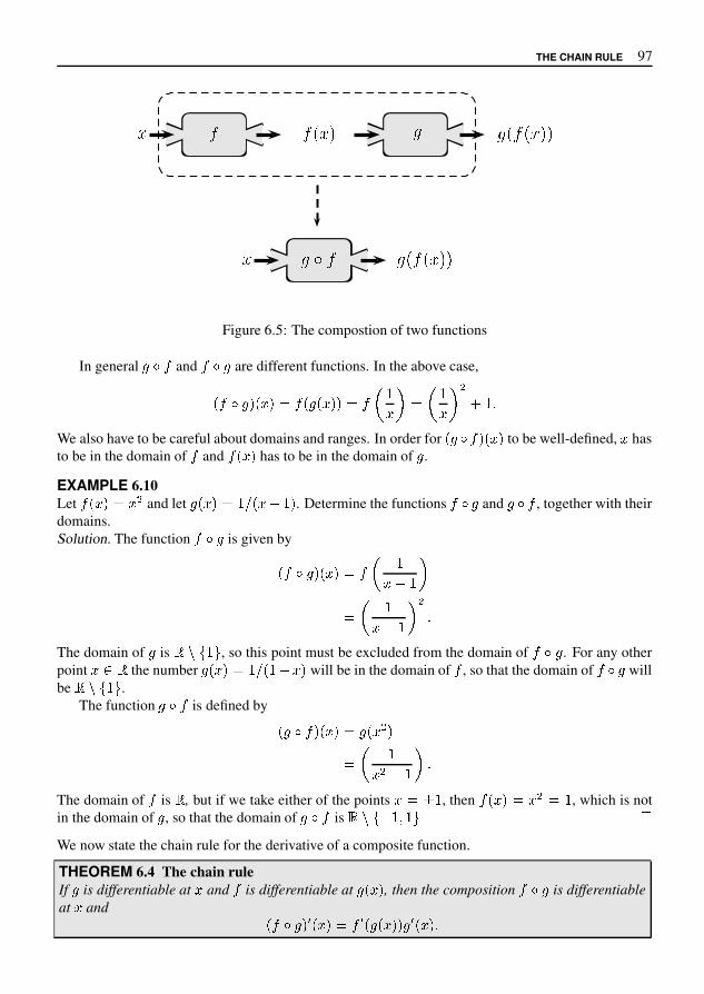
THE CHAIN RULE 97
�� � � � � � � � � � � � �
� � �� � � � � � � �
Figure 6.5: The compostion of two functions
In general � � � and � � � are different functions. In the above case,
� � � � � � � � � � � �� � � � �� � � � � "We also have to be careful about domains and ranges. In order for � � � � to be well-defined, � hasto be in the domain of � and � � has to be in the domain of � .
EXAMPLE 6.10Let � � � � � and let � � � � & � ) � . Determine the functions � � � and � � � , together with theirdomains.Solution. The function � � � is given by
� � � � � � � �� ) � �� � �� ) � � � "
The domain of � is 0 1 2 � 5 , so this point must be excluded from the domain of � � � . For any otherpoint � 7 0 the number � � � � & � ) � will be in the domain of � , so that the domain of � � � willbe 0 1 2 � 5 .
The function � � � is defined by
� � � � � � � � � � �� � ) � � "
The domain of � is 0 , but if we take either of the points � � ? � , then � � � � � � � , which is notin the domain of � , so that the domain of � � � is 0 1 2 ) � C � 5 EWe now state the chain rule for the derivative of a composite function.
THEOREM 6.4 The chain ruleIf � is differentiable at � and � is differentiable at � � , then the composition � � � is differentiableat � and � � � F � � � F � � � F � "
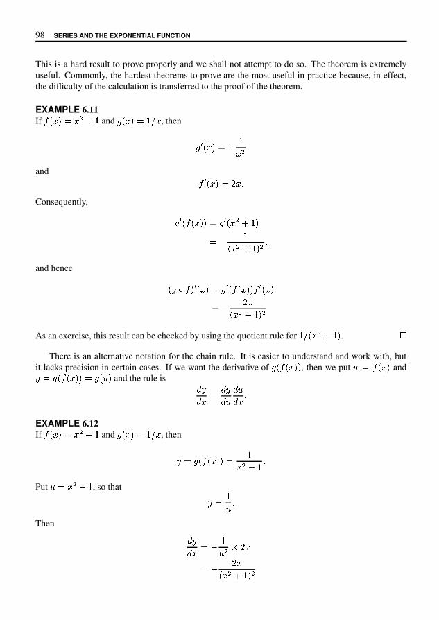
98 SERIES AND THE EXPONENTIAL FUNCTION
This is a hard result to prove properly and we shall not attempt to do so. The theorem is extremelyuseful. Commonly, the hardest theorems to prove are the most useful in practice because, in effect,the difficulty of the calculation is transferred to the proof of the theorem.
EXAMPLE 6.11If � � � � � � � and � � � � � � , then
� � � � � �
� �
and� � � � � � � �
Consequently,
� � � � � � � � � � � � � � �
�
� � � � � �
and hence
� � � � � � � � � � � � � � � � � � � � � �
�� �
� � � � � �
As an exercise, this result can be checked by using the quotient rule for � � � � � � . #
There is an alternative notation for the chain rule. It is easier to understand and work with, butit lacks precision in certain cases. If we want the derivative of � � � � � � � , then we put $ � � � � and' � � � � � � � � � $ � and the rule is
* '* �
* '
* $* $* �
�
EXAMPLE 6.12If � � � � � � � and � � � � � � , then
' � � � � � � �
� � � �
Put $ � � � , so that
'
$�
Then
* '* �
�
$ �- � �
�� �
� � � � � �

PROPERTIES OF THE EXPONENTIAL FUNCTION 99
EXERCISES 6.6
In exercises 1–6 you are given two functions � and � . In each case, find the compositions � � � and� � � .
1. � � � � � � � � � � � � � � 2. � � � � �� � � � � � � � � � � �3. � � � � � � � � � � � � � � � 4. � � � � � � � � � ! � ! � �5. � � � � $ � � � � � � � � � � � ' 6. � � � � � ( � � � � � )
Differentiate each of the functions in Exercises 7–10.
7. � � � � � � � � � � 8. � � � � � � � � ( ,9. � � � � � � ( � $ � � � � , 10. 0 � 1 � 3 1 � �1 4 5
6.7 PROPERTIES OF THE EXPONENTIAL FUNCTIONAs we have already mentioned, the exponential function satisfies a number of algebraic identitieswhich can be used to simplify computations. The following theorem summarises the main ones.
THEOREM 6.5For any real numbers 6 and 7 , the exponential function satisfies the following identities.
8� � � � 6 � 7 � � � � � 6 � � � � 7
8� � � � � 6 � �
� � � � 6 8� � � � 6 > ?
8� � � � 6 � 7 � � � � � 6
� � � � 7 The trick to deriving the properties of the exponential function in Therorem 6.5 is to consider the
function defined on A by � � � � � � � � � � � � � 6 � 7 � � �where 6 and 7 are any real numbers. Using first the product rule and then the chain rule, we have
DD � � � � � � � � � � � 6 � 7 � � � � � � � � DD � � � � � � 6 � 7 � � � DD � � � � � � � � � � � 6 � 7 � � � � � � � � � � � � 6 � 7 � � DD � � 6 � 7 � � � � � � � � � � � � 6 � 7 � � � � � � � � � � � � 6 � 7 � � � � � � � � � � � � � � � 6 � 7 � � � ? J (6.13)
This result holds for all real numbers 6 , 7 and � . We know that if a function is constant then itsderivative is zero. It is an important result that a partial converse is also true.

100 SERIES AND THE EXPONENTIAL FUNCTION
THEOREM 6.6If the derivative of a function is zero on an open interval � (possibly � � � ), then the function is
constant on � .
This result is very important and surprisingly difficult to prove and we shall not do it here. Neverthe-less, we shall make use of it in equation (6.13) and in many later situations. Since � and � � are definedeverywhere on � , this equation implies that � � � � � for some constant � . Thus
� � � � � � � � � � � � � � � � �
This is true for all values of � , so to find � , we substitute any value of � and solve for � in terms of �and � . The obvious value to try is � � � , since we know � � � � � � " . This gives
� � � � � � � � � � � � � � %
so that � � � � � � � � � and hence
� � � � � � � � � � � � � � � � � � � � � � � (6.14)
Finally, let � � � in this last equation to get
� � � � � � � � � � � � � � � � � � %
which is the first identity in Therorem 6.5.We can also extract the second identity in Theorem 6.5 from equation (6.14). If we put � � � and
� � � we find� � � � � � � � � � � � � � � � � � " %
so that
� � � � � � �"
� � � � ��
If � 2 � , then � � � � � 5 � as can be seen from the series defining � � � � � . This last equation thenimplies that � � � � � � 5 � . Thus � � � � � 5 � for all � . The proof of the final identity of Theorem 6.5is left to you as an exercise.
The properties of the exponential function in Theorem 6.5 enable us to develop an alternative wayof looking at this function. We first define a number 6 by letting 6 � � � � " � . Calculations with thepower series give 6
�� : � ; " > : > . The number 6 is an irrational number and it plays a key role in the
applications of calculus to the real world. Once we have defined 6 , we have the following.
� � � : � � � � � " � " � � � � � " � � � � " � � 6 @
and similarly � � � A � � 6 B , � � � C � � 6 D ,. . .Also
� � � � : � �"
� � � : ��
"6 @
� 6 F@
and similarly � � � � A � � 6 F B , � � � � C � � 6 F D % � � � These results, together with the result � � � � � �" , show that
� � � I � � 6 J
for all integers I .

PROPERTIES OF THE EXPONENTIAL FUNCTION 101
How would we calculate the square root of the number � ? We have as yet given no rule for calcu-lating the square root of any number which is not an exact square, but we can now give a procedurefor calculating � � . We have
� � � � � � � � � � � � � � � � � � � � � �so that
� � � � � � � �To calculate � � � � and hence � � , we use the power series for the exponential function. We cansimilarly deal with any rational power � � � � �
, where � and�
are integers. We have
� � � � � � � � � � � � � � � � � � � �� terms
"� � � � � $ � � % "
�
� � � � � � �Hence � � � � � � � � � � � � � � � � � �so that we can calculate � � by using the series for � � � � . Finally, when � is an irrational number, wesimply define � � by letting � � � � � � � . We then have
� 1 � � � � 3for all 3 5 7 .
EXAMPLE 6.13Calculate � � to 4 decimal places.Solution. We have
� � � 3 � � � 3 � 3 �: < � 3 >? < � The error A C satisfies A C E 3 C
F G � < F G 3 �If we put 3 � � � : , then we find A K L M � M M M M ? , so that
� � � � � �: � � �: O P < �� � � P Q R T :to 4 decimal places.
EXAMPLE 6.14Find the derivatives of � � � U 3 and � � � G U 3 �Solution. We use the chain rule, together with the result � � � W 3 � � � � 3 .
YY 3 � � � U 3 � � � � U 3 YY 3 U 3 � U � � � U 3 �

102 SERIES AND THE EXPONENTIAL FUNCTION
Similarly�
� �� � � � � � � � � � � � � � � � �
�� �
� � � � � � � � � � � � � �
Another way of writing these results is
�� �
� � � � � � � � (6.15)
�� �
� � � � � � � � � � � (6.16)
EXERCISES 6.7
Differentiate the functions given in Exercises 1–8.
1. � � � � ! � 2. � � � � � 3. # � & � � '
(� �
�* � � �
� 4. # � � � � � - � � ! � � 0
5. # � � � �� � � -� � * -
6. � � � ! � ( �
7. 4 � � � � 6 � � � 9 � 9 ' 8. 4 � � � �� �
- * �
9. Using the series definition of the exponential function, find an approximation for � < ( accurate to
3 decimal places. This means that your maximum error must be less than 0.0005.
10. Find an approximate value of - = � to 3 decimal place accuracy, using the series expansion for theexponential function.
11. How many terms of the exponential series would we need in order to find � > accurate to0.0000000001, that is, accurate to - @ � ' < ?
12. Find an example of a function # for which # A � � � � @ for all � in the domain of # , but for which# � � � is not a constant. Can you reconcile this result with the statement of Theorem 6.6?
6.8 SOLUTION OF THE AIR PRESSURE PROBLEMIn Section 6.1, we found the differential equation for the air pressure problem to be
C A � D � � � @ � @ @ @ - @ F C � D � � @ � @ - H � C � @ � � - @ - H � (6.17)
The constants are awkward to deal with, so let us replace them by symbols for ease of working. Wewrite
C A � D � � � C � D � * L � C � @ � � � �
with � @ � @ @ @ - @ F , L � � @ � @ - H and � � - @ - H . Equations of this form are applicable to problemsother than the air pressure problem, so let us emphasize this generality by writing � � # � � � , where #has no particular physical interpretation. The differential equation to be solved is
� A * � � L � � � @ � � � � (6.18)
We could solve this equation by a power series method, but since we have now developed an impres-sive amount of mathematics in defining the exponential function, let us try to make use of some ofit.

SOLUTION OF THE AIR PRESSURE PROBLEM 103
We solve equation (6.18) by working through several steps. First we solve the case when � � � ,that is, we solve the equation � � � � � � � (6.19)
At this stage we will ignore the initial condition � � � � � � . To solve the equation we make use ofthe result (6.16), which shows that � � � � � � is a solution of the differential equation. Sometimesequations have more than one solution, so we have to ask whether the solution � � � � � � is the onlysolution of equation (6.19). Suppose that � � � � � is some other solution, so that � �� � � � � " � � � � � .Then, by the quotient rule,
$$ � & � � � � �� � � � ' � (� � ) � � & � � � � � �� � � � " � � � � � $$ � � � � � � � '� (� � ) � � , � � � � � " � � � � � � " � � � � � � " � � � � � � � 2� � �
This means that � � � � �� � � � � 4 5for some constant
4and so � � � � � � 4 � � � � �
This result shows that every solution of � � � � � � must have this form. We have reached animportant result which is worth some discussion. We call
� � 4 � � � �the general solution of the equation � � � � � � , since every solution has this form. If we know theinitial condition � � � � � � 9 , then it follows that
4 � � 9 , so that
� � � 9 � � � �is a solution of the initial value problem � � � � � � , � � � � � � 9 . We call � � � 9 � � � � a particularsolution of � � � � � � . In summary we have the following result.
The initial value problem � � � � � � � � � � � � 5 � � � � � � 9 (6.20)
has the solution � � � 9 � � � � �Next we move on to the more general equation
� � � � � � �The strategy here is to replace the constant
4by a function � � � � . The idea behind this is as follows:
1. � � 4 � � � � satisfies � � � � � � .
2. If we replace the constant4
by a function � � � � , we may be able to choose � � � � so that theright hand side comes out to � rather than zero.

104 SERIES AND THE EXPONENTIAL FUNCTION
This is an instance of a general procedure for solving differential equations we will encounter againlater. It is known as the method of variation of parameters or variation of constants. The idea is tosolve a simpler problem and then replace the constants by functions in a trial solution for the morecomplex problem. If we substitute � � � � � � � � �into the equation � � � � � � � �we get
� � � � � � � � � � � � � � � � � � � � � � � � � � � � �so that
� � � � � � � � � �and hence
� � � � � � � � � �We are now looking for a function � � � whose derivative is � � � � . It is not difficult to verify, usingthe chain rule, that
� � � � �� � � � � �is such a function, where
�is a constant. Thus the solution we are seeking has the form
� � � � � � � � � � ! �� � � � � � " � � � �� �� � � � � � � �
This is easily checked to be a solution of � � � � � � � for any value of the constant'
. If we now makeuse of the initial condition � � ) � � , we have
' � � � � - � and so
� � �� � ! � � �� " � � � � �This is another result worth summarising:
The initial value problem � � � � � � � � � � ) � � 2 (6.21)
has the solution
� � �� � ! � 2 � �� " � � � � �The air pressure equation (6.17) has the same form as equation (6.21). Using the values � �) � ) ) ) 7 ) 9 , � � � ) � ) 7 < , = 2 � � � 7 ) 7 < in equation (6.17) gives
= � A � � 7 D ) � 7 7 < < � � 2 � 2 2 2 G 2 H
as the solution to the air pressure problem. We can check that this will reproduce the results ofTable 6.1. In computing the exponential terms we could use the power series expansions, but almostany calculator will have the calculation hardwired into it, so that we can evaluate the exponentials at

SOLUTION OF THE AIR PRESSURE PROBLEM 105
the touch of a button. (But remember, the designers of the calculator needed to have access to muchof the theory of this chapter.)
The unifying thread of this chapter has been the problem of finding an equation for the variationof air pressure with respect to height and we have developed an impressive amount of mathematicsto reach the solution. The big payoff, however, is not that we can now solve the air pressure prob-lem. Rather, it is that the mathematics we have developed is useful and applicable in a wide varietyof seemingly unrelated problems. One of these is given in the example below. Others appear inExercises 6.8.
EXAMPLE 6.15A tank initially contains 100 litres of water in which 5 kilograms of salt is dissolved. Pure water ispumped into the tank at a rate of 2 litres per second. The mixture in the tank is pumped out at thesame rate. Set up and solve the differential equation for the amount of salt � in the tank at time � .
Solution. Let � be the amount of salt in the tank at time � . Then the initial condition is � � � � � andthe amount of salt per litre is � � � � � . Let
� � be change in the amount of salt in the tank during thetime interval � � � � � � � � , where
� � is assumed to be small. We have
� � � � �� � � � � � �
and this approximation becomes increasingly accurate as we let� � approach zero. We rearrange this
equation in the form � �� � � � �� � � #
Using the Leibniz approach to differentiation (page 46), we let� � approach zero and the equation
becomes$ �
$ � � �� � #
This is of the same form as equation (6.20) with & � � � � . The solution is
� � � � � + , �� - . #
EXERCISES 6.8
The exercises in this section can (and should) be done without the use of logarithms, which we con-sider in Chapter 9.
A simple model of population growth assumes that the population / grows at a rate which is propor-tional to / . That is
$ /$ � 0 / �
where 0 is a positive constant. This is often called the exponential or natural growth equation. Itapplies if birth and death rates are constant.
As well as representing population growth, the above differential equation (possibly with 0 2 � ) hasmany other applications, including compound interest, radioactive decay and drug elimination fromthe bloodstream.
Use the exponential growth equation in exercises 1–4.

106 SERIES AND THE EXPONENTIAL FUNCTION
1. A city had a population of 25 000 in 1980 and a population of 30 000 in 1990. What will thepopulation be in the year 2000?
2. The number of bacteria in a certain culture increases at a rate proportional to the number present.Suppose there are 1000 bacteria present initially and 1600 after 1 hour. How many will be presentafter 3 hours?
3. The drug sodium pentobarbitol is used for anesthetising dogs. The dog is anesthetised as long asits bloodstream contains at least 45 mg of the drug per kilogram of the dog’s body weight. Sup-pose that sodium pentobarbitol is eliminated from the dog’s bloodstream at a rate proportional tothe amount of the drug present, and that half the drug is eliminated after 5 hours. How much ofthe drug should be administered in order to anesthetise a 25 kg dog for 2 hours?
4. A curve passes through the point � � � � and has the property that the slope of the curve at anypoint is three times the value of the � coordinate of . Find the equation of the curve.
5. Let � be the temperature of a body. Newton’s law of cooling states that the time rate of change ofthe temperature � � � of a body is proportional to the difference between � and the temperature� � of the surrounding medium. Show that
� �� � � � � � � � � � �where � � � is a constant.
Solve this equation in the following two ways:
(a) Use equation (6.21) in the text.
(b) Put � � � � � � and show that the equation becomes
� �� � � � � � !Solve this equation and replace � by � � � � in the solution. What is the physical interpre-tation of � ?
6. Solve the initial value problem � # � � & � ) + , � � � � � in the following way.
(a) Write the differential equation as
� # � � & . � � +& 1 !(b) Put 2 � � � + 8 & , solve the resulting initial value problem and replace 2 by � � + 8 & in the
solution.
7. A cake is removed from an oven at a temperature of 150 � C and left to cool. After 30 min, thetemperature of the cake is 90 � C. What will the temperature be after 2 hours? Assume that theroom temperature is 25 � C.
SOLUTION OF THE AIR PRESSURE PROBLEM 107
8. A tank initially contains 100 litres of pure water. Water containing salt at a concentration of0.1 kg/litre is pumped into the tank at a rate of 5 litre/min. The mixture in the tank is pumped outat the same rate. Show that the differential equation for the amount of salt � in the tank at time �is
� �
� �� � �
�
�
Hence find the amount of salt in the tank after 10 min.
9. A lake has a volume of 1 billion cubic metres of water, with an initial pollutant concentration of0.25%. The average daily inflow of water into the lake is 1 million cubic metres of water, with anaverage pollutant concentration of 0.05%. The average daily outflow of well mixed water fromthe lake is equal to the average inflow. What will be the concentration of pollutant after 5 years?
10. Using Mathematica, check that the solution to the air pressure problem
� � � � � � � � � � �� � � � � �
�� � �
obtained above will closely reproduce the values in Table 6.1.The atmosphere only extends a finite distance above the surface of the earth. Consequently, wewould expect the pressure to approach zero as the height increases indefinitely. Suggest reasonswhy this does not happen for the above solution.

This page intentionally left blank

CHAPTER 7
TRIGONOMETRIC FUNCTIONS
In this chapter we consider the vibrating cables of the Anzac Bridge. A full analysis of the problemwould take us well beyond the mathematics in this book, but we can still make progress by makingsome assumptions and simplifications.
7.1 VIBRATING STRINGS AND CABLES
The problem to be considered is the vibration of a cable or string with fixed end points. On a large scalethis could apply to the Anzac Bridge, while on a small scale it could apply to a musical instrument,such as a violin or guitar. The numerical information we want to derive is the frequency at which thecable vibrates. The frequency we are considering here is the frequency of vibration when there areno outside influences. This is called the natural frequency. If some outside influence tries to make asystem vibrate with its natural frequency, then the system will readily do so. To make it vibrate at adifferent frequency is more difficult, a problem we will consider in detail in Chapter 8.
Let us consider a vibrating string or cable. The mass is spread out along the string. If the totalmass is
�and the string has length � , then its mass per unit length is � �
�� � . To analyse the
motion of the string, we have to consider each part of it, but this requires mathematics beyond thatwhich we will develop in this book. This is a task for a later subject. Instead, we shall make a simpleapproximation and assume that the mass of the string is concentrated in a single body at the center ofthe string (Figure 7.1). The string vibrates because it is under tension and this tension exerts a forceon the body. We denote the tension in each half of the string by � � and � � respectively and we let �be the displacement of the centre of the string from the equilibrium position.
The tension in each half of the string can be split into two parts, a horizontal component anda vertical component. Since the body does not move horizontally, the two horizontal components� �� and � �� must be equal and opposite to each other and we can ignore them as far as the verticalmotion is concerned. It follows that the tensions � � and � � are equal and hence that the two verticalcomponents are equal. Let � be the common value of � � and � � and let � � be the value of the verticalcomponent. The two vertical components add up to give a total force of � � on the body. Newton’ssecond law of motion implies that
� � �
� �� � � � � (7.1)

110 TRIGONOMETRIC FUNCTIONS
�
� � �
� ��� �� �
�
� � � �� �� �
� � � � � �
�
Figure 7.1: A vibrating string or cable
Using similar triangles in Figure 7.1, we have
� �� �
� � � � � � � ��
If � is small, then
� � � � � � � � �� �
so for small � ,
� �� �
� � � �
that is,
� � � � �� �
We shall assume that the error in this approximation is negligible for small � and write
� � � � �� �
Using this result in equation (7.1) gives us
�� � �
� � � � � � �
� �
or
� � �� � �
� � � �
��
� � � �� � � �
TRIGONOMETRIC FUNCTIONS 111
We shall write this as� � �
� � �� � � � � �
where
� ��� � �
��
We shall assume that the motion commences at � � with the mass displaced by � � and with velocity� � . Thus � � � � � � and � � � � � � � , which leads to the initial value problem
� � �� � �
� � � � � � � � � � � � � � � � � � � � �
The differential equation in this problem is known as a second order differential equation , since thederivative appearing in the equation is of second order. We will discuss solutions of this equation inthe next section.
7.2 TRIGONOMETRIC FUNCTIONSIn the previous section, we arrived at the initial value problem
� � �� � �
� � � � � � � � � � � � � � � � � � � � � (7.2)
To solve this equation, we use the method of infinite series as developed in Chapter 6. Polynomialfunctions will fail for the same reasons that they failed in Chapter 6. Let us use, as a trial solution, afunction defined by a power series:
� � � � �%�
� & �' � � � � (7.3)
The problem is to determine the coefficients ' � . On differentiating twice, using Theorem 6.2, we have
� � �� � �
�%�
� & �
) � ) , . � ' � � � 1� (7.4)
You may be puzzled by the fact that the sum now goes from ) � � instead of from ) � . The reasonis easy to see if we first expand the first few terms of the sum (7.3) to get
� � � � � ' � � ' � � � '�
� � � ' 5 � 5 � ' 6 � 6 � 7 7 7 �
and then take the second derivative
� � � � � � � � '�
� < � � ' 5 � � > � < ' 6 � � � 7 7 7 �%�
� & �
) � ) , . � ' � � � 1� �
Since the derivative of a constant is zero, one term drops out for each differentiation. We substituteequations (7.4) and (7.3) into equation (7.2) to get
%�� & �
) � ) , . � ' � � � 1� � � �
%�� & �
' � � � � �
112 TRIGONOMETRIC FUNCTIONS
that is, replacing � by � � � in the first sum,
��
� � � � � � � � � � � � � � � � � � � � ��� � � � � � � � � �
Hence ��� � �
� � � � � � � � � � � � � � � � � � � � � � � � � that is,
��� � �
� � � � � � � � � � � � � � � � � � � � � � � �If we equate coefficients of � � on both sides of the equation for � � � � & � � � , we find
� � � � � � � � � � � � � � � � � � � � � � � � & � � �which shows that � � � � � * � � � � � � � � � � � � � (7.5)
Equation (7.5) is called a recurrence relation; it gives the coefficient � � � � in terms of � � . Sinceequation (7.5) relates each coefficient to the second one before it, the even-numbered coefficients( � � � � � , � - � � � ) and the odd-numbered coefficients ( � . � / � 0 � � � ) will be determined separately.For the even-numbered coefficients, we have
� � � * � � � �� � � � * � � � �� 1 � , � * � � � �3 � & � � � � ,3 1 � - � * � , � �5 � 6 � * � � � -5 1 and in general
� � � � * � � � � � � 1 � � � � � � � � � & � � � (7.6)
Similarly, for the odd-numbered coefficients, we have
� / � * � . � �& � � � * � . � �& 1 � 0 � * � / � �6 � 3 � � . � ,6 1 � 9 � * � 0 � �: � 5 � * � . � -: 1 and in general
� � � � . � * � � � � � � � � 1 � � � � . � � � � & � � � (7.7)
Substitution of equations (7.6) and (7.7) into equation (7.3) gives
= � � � � � A � * � � � �� 1 � � � � ,3 1 * E E E F� � .� A � � * � � � /& 1 � � � � 06 1 � E E E F
(7.8)
TRIGONOMETRIC FUNCTIONS 113
The two series in parentheses are extremely important. They are functions which you may havealready met, although the connection will not be obvious at this stage. We define the sine and cosinefunctions as follows:
DEFINITION 7.1 The sine and cosine functionsFor all � � � , we define
� � � � � � � �� � � � �
� � � � �� � � � � � �
��
� � � � # % �
' ) � # % � � + � , - (7.9)
. 0 � � � # � � +' � � � 5
6 � � � 89 � � � � � �
��� � �
� # % � ' ) % � � + � : (7.10)
Of course, we have to verify that the series in Definition 7.1 actually converge. We can do this bymeans of the ratio test. The general term of the sine series is
; � � � # % � ' ) � # % � � + � , - <
so that
= � >� ? � AAAA
; �; � C - AAAA
� = � >� ? � AAAAA
� # % � ' ) � # % � � + � , - � � # % � C -
' ) � # % � � + � C - AAAAA� = � >� ? � F � + F ' ) � # % ' ) � # %
� G :Since this limit is less than 1 for every � � � , the series converges by the ratio test and the radius ofconvergence is infinite. Thus � � � has domain � . A similar calculation shows that the series for . 0 � �converges for all � � � and so the domain of . 0 � � is � .
Using Definition 7.1, equation (7.8) can now be written
K � % � ; � . 0 � � � � ; -� � � � � : (7.11)
The arbitrary constants ; � and ; - can be found using the initial conditions. Finding ; � is easy. We put� � G in equation (7.8) and find K G % � ; � . To find ; - , we differentiate equation (7.8) with respect to� and then put � � G . This procedure is justified by Theorem 6.2. We find
K P � % � ; � � � + � � � � � 5� � � � � � 8
� � � � � � % � ; -� � � � � � +� � � � � � 5
6 � � � � � % :Putting � � G gives K P G % � ; - , so that ; - � K - . The final solution to the initial value problem (7.2)is thus
K � % � K � . 0 � � � � K -� � � � � : (7.12)
EXERCISES 7.2
1. Use the ratio test to show that the series (7.10) converges for all real numbers � .
114 TRIGONOMETRIC FUNCTIONS
2. The ends of a string under tension are fixed at two points�
and�
. The distance� �
is 2 m, themass per unit length of the string is 0.1 kg and the tension in the string is 2 N. The centre of thestring is displaced a distance of 5 cm from its equilibrium position and then released. Find thevalue of the constant � in equation (7.12) and use this equation to find the displacement of thecentre of the cable after 2 seconds.
7.3 MORE ON THE SINE AND COSINE FUNCTIONSDefinition 7.1 provides the basis for all calculations with � � � � and � � � . These functions have beenintroduced because they provide solutions for the differential equation (7.2). This differential equationarises in all oscillation problems. The power series definitions enable function values to be calculatedto any desired accuracy and so the functions are well-defined. We shall later relate these trigonometricfunctions to the properties of triangles. These properties are used to define trigonometric functions inelementary mathematics, but it should be noted that the definitions in this form do not enable functionvalues to be calculated to arbitrary accuracy.
The series for � � � � and � � � each have the property that successive terms have opposite signsfor any value of � . Such a series is called an alternating series. There is a simple rule for calculatingthe error term for such a series, as long as the terms are decreasing in magnitude. The error, inabsolute value, is less than the first term omitted. In the case at hand the terms of either series mayinitially increase for some values of � , but as long as we take enough terms, they will eventually startto decrease. For example, if � � � in the sine series, we get
� � � � � � � � �� � � � �
� � � � �� � � " " "
� � � % ' (� � * +, � � � � . ,, ( / 0 � " " "
If the value of � is large, there may be many increasing terms before a decrease begins. To see that theterms will always start to decrease eventually, we note that each term is obtained from the previousone by multiplying it by an expression of the form
� � (1 3 5 � % 7 1 3 5 � 3 7 9
For large enough 5 the absolute value of this term will be less than 1. Thus to calculate � � � , we usethe following rule:choose 5 so that
� (1 3 5 � % 7 1 3 5 � 3 7 : %
and then calculate the terms� ( � = (
1 3 5 � 3 7 � > � ( � = 01 3 5 � � 7 � > 9 9 9
until we find one whose magnitude is less than the required error. Suppose this term is
� ( A1 3 C 7 � 9
Then
� � � � % � � (3 � � � 0
� � � " " " � 1 � % 7 A � ( A I (1 3 C � 3 7 � >
MORE ON THE SINE AND COSINE FUNCTIONS 115
with an error of less than� �
�
� � � �
EXAMPLE 7.1Suppose we wish to evaluate � � � � � � with an error of less than � � � � � . Since
� � � �� �
� � �
all terms after the first are decreasing and we calculate successive terms. We find
� � � �� �
! � � � � � $
Thus we omit all terms after the second to get
� � � � � � � '� � � �
� �! � ( ) �
with an error of less than 0.00007. In terms of inequalities we have
� ( $ ( ( * � � � � � � � � ( ) � � $
It is common to write results such as this in the form
� � � � � ! � ( ) � � � 0 � � � � � $
EXAMPLE 7.2To evaluate � � � � with an error of less than 0.0001, we first look at terms of the form
� �� � � 3 � � � � 3 �
This gives
� ! � �
� :* < �
> �
� ! � �
� :� < B
� �
This means we have to evaluate the terms
� C: �
�� D
) ��
until one of them is less than the allowable error. We find
� E C� : �
! � � � � � �
� E D� ) �
! � � � � � � �
so that
� � � � � � '� �
� �3
� �� �
' F F F 3� E C
� : � ! ' � : B * : �
with an error of less than � � � � � . I

116 TRIGONOMETRIC FUNCTIONS
These calculations can get very lengthy as the argument of the function gets larger, but as we shallsoon see there are properties of the functions which shorten them considerably. These properties haveto be deduced from the power series definitions or from the original differential equation (7.2).
Some properties are easily deduced from the power series definitions. If we put � � � in theseries for � � � , we find � � � � � . Similarly, � � � � � � . If we replace � by � � in the sine series,we see that � � � � � � � � � � � , and similarly, � � � � � � � � � � � � . There is, however, a fundamentalproperty of the sine and cosine functions which is not at all obvious from either the power series or thedifferential equation and that is their periodicity . This means that there is a particular number � suchthat � � � � � % � � � � � � � and � � � � % � � � � � � for all values of � . We shall need some preliminaryresults before we can demonstrate this.
The first result we need is contained in Definition 7.1. If we use the rule for differentiation of apower series to differentiate equation (7.9) with respect to � , we find
++ � � � � � � � � � � 01 2 % � 45 2 � � 78 2 % ; ; ; =while if we differentiate equation (7.10) with respect to � , we find
++ � � � � � � � � � ? � � � AB 2 % � CD 2 � � EF 2 % ; ; ; H IBy comparing these equations with Definition 7.1, we reach the following important theorem.
THEOREM 7.1 Derivatives of the sine and cosine functionsFor all � K L , we have
++ � � � � � � � � � � �++ � � � � � � � � � � � � I
The next theorem states two important properties of the sine and cosine functions.
THEOREM 7.2 Identities for the sine and cosine functionsFor all real numbers P and Q we have
� � � P % Q � � � � P � � � Q % � � � P � � Q� � � � P % Q � � � � � P � � � Q � � � P � � Q IThis theorem can be proved by a similar method to that used to show � � � � P % Q � � � � � P � � � Q .
We begin with the function
X � � � � � � � � � � � P % Q � � � % � � � � � � � P % Q � � � IThen, using the product rule and the chain rule,
X Y � � � � � � � � � � � � P % Q � � � % � � � � � � P % Q � � �� � � � � � � P % Q � � � � � � � � � � � � P % Q � � �� � I

MORE ON THE SINE AND COSINE FUNCTIONS 117
Since � � � � � , we must have � � � � � for some constant � . Hence
� � � � � � � � � � � � ! � � � � � � � � � � � � ! � '
If we put � � we get � � � � � � � � , where we have used the results � � � � , � � � � / . Putting� � � then gives the first identity in Theorem 7.2. The proof of the second one is similar. If wereplace by ! in this theorem and use the results � � � � ! � � � � � � , � � � � ! � � ! � � � � , we deducethe following result.
THEOREM 7.3 Identities for the sine and cosine functionsFor all real numbers � and we have
� � � � � ! � � � � � � � � ! � � � � � � �
� � � � � ! � � � � � � � � � � � � � � � � '
If we put � � � � in the second identity in Theorem 7.3, we get
� � � � � ! � � � � � � � � � � � � � � � � � � � '
Hence� � � @ � � � � � @ � � / '
Finally, from Theorem 7.2 we can get the following double angle formulas by putting � � .
� � � D � � D � � � � � � � �
� � � D � � � � � @ � ! � � � @ � '
using the result � � � @ � � � � � @ � � / in this last equation, enables us to deduce that
� � � D � � D � � � @ � ! /
and
� � � D � � / ! D � � � @ � '
All of these results have been obtained purely from the power series definitions of the functions.
EXERCISES 7.3
Prove the trigonometric identities in Exercises 1–4.
1. � � � ��
� � � ��
@ � � � � ��
! � � ��
@ � D
2./ ! � � � K
� � � K�
� � � K/ � � � � K
3./
/ ! � � �� �
// � � � �
� �D
� � � @�
4.� � � L K � � � � L K
� � � K � � � � K� / ! � � � K � � � K
In Exercises 5–12, find the derivative of the given function.

118 TRIGONOMETRIC FUNCTIONS
5. � � � � � � � � 6. � � � � � � � � � � � � �7. � � � � � � � 8. � � � ! � � � � � 9. � � � � � � �# $ � � � � 10. � � � � � # ) � � � � � +
11. � � � � � � � � $ , � � � � 12. � � � � / � � � 1 � 3 4# 1 � 4 813. Let � and � be differentiable functions such that � : � � � $ � � � � and � : � � � � � � � for all � .
(a) Prove that � � � � � ) � � � � � ?, a constant
(b) Suppose there is a number @ such that � � @ � # and � � @ � 4 . Find the value of?
.
(c) Give an example of a pair of functions with these properties.
14. Show that � $ DE � � � � � � satisfies the differential equation
� : : ) H � � � � � 815. Show that � $ D+ ! J � � � � satisfies the differential equation
� : : $ � � : $ � ! J � � � � 816. Show that � L ! J ) M ! N J $ ! J � � ! N J satisfies the differential equation
� : : $ � ! N J � � ! N J ) � � � ! N J 1where
Land
Mare arbitrary constants.
17. A simple pendulum consists of mass Q suspended from a fixed point by a light inelastic string,as in the diagram.
�
�
The angular displacement� � � � of the mass at time � is given by
� � � � L � � � � � � ) � � 1where
L, � and � are constants.
TRIANGLES, CIRCLES AND THE NUMBER � 119
(a) Show that�
satisfies the differential equation� � � � � � � � � .
(b) Show that�
can be written in the form
� � � � � � � � � � � � � � � �
where � and � are constants.
7.4 TRIANGLES, CIRCLES AND THE NUMBER �You will already have met the sine and cosine functions in connection with triangles. The functionswe have defined in terms of power series are the same functions, but we have not yet shown this.Notice, that while the triangle definitions may look simpler than the power series definitions, they donot give any systematic method for calculating function values. These functions can also be definedby using the unit circle, but this is just a generalisation of the triangle definitions. The number � arisesnaturally in connection with trigonometric functions and here we can also make connections with thepower series definitions.
7.4.1 Trigonometric functions defined by triangles
In this section we connect the series definitions for the trigonometric functions with the more familiardefinitions in terms of the ratios of various sides of a right-angled triangle.
Suppose we have a particle moving around a circle of radius � such that the velocity has constantmagnitude " � . At each instant the direction of the velocity is tangential to the circle (Figure 7.2).The velocity can be resolved into a component # parallel to the $ axis and a component parallelto the % axis. We can get the magnitudes of # and by using the fact that triangles & ' (
and( � )
are similar, but we have to be careful about the sign of these quantities. Let’s look at the magnitudesfirst.
In triangles & ' (and
( � ) , we have
* ( � ** ( ) * � * ' ( *
* & ( * and* � ) *
* ( ) * � * & ' ** & ( * ,
Hence* # *
* * � * % ** � * and
* ** * � * $ *
* � * �
so that
* # * � * % *� and * * � * $ *
� ,
In the diagram shown, # 1 � so * # * � 4 # , while % is positive. Hence
# � 4 %� ,
You should convince yourself that # and % always have opposite signs, no matter where the particlemay be on the circle, so this equation always applies. Similarly, always has the same sign as $ , sothat
� $� ,

120 TRIGONOMETRIC FUNCTIONS
�
�
�
�
�
�
� �
�
�
� ��
�
�
Figure 7.2: A particle moving in a circle
On the other hand, from the definition of velocity we know that � � � and � � � , so
� � � � � � (7.13)
� � �� � (7.14)
We differentiate equation (7.13) and make use of equation (7.14) to get
� � � � �� �
� �
If we write � � � � � , then this last equation becomes
� � � � � � " � (7.15)
If we assume that the particle starts from the point�
, then � $ " & � � and � $ " & � " . With these initialconditions the solution of equation (7.15) is � � � - / 0 � 1 and so � � � � � 0 6 7 � 1 . Comparing thetwo expressions we have found for � gives the result
0 6 7 � 1 � � �
Finally we note that� � arc
� �
� � � 1� � � 1 �
Hence0 6 7 � �
� �

TRIANGLES, CIRCLES AND THE NUMBER � 121
Similarly,
� � � � � ��
These last two equations show that the functions we have obtained as power series from the differentialequation are indeed the familiar functions from elementary trigonometry.
7.4.2 The number �
Consider points where � � � � � � . We know that � � � � � � and it can be verified as an exercise that� � � � � � � � � � . The cosine function is differentiable and so continuous and hence there will be atleast one number � � between 0 and 2 where � � � � � � � . Let us consider the smallest positive numbersatisfying � � � � � � . For historical reasons, this number is denoted by ! � . Thus
� � � ! � � �
How do we calculate the number ? We begin by showing that � � � � is a decreasing function between0 and 2, that is, we wish to show that the graph of � � � � on $ � % � ( looks like the graph in Figure 7.3.
�
�
� �
)
*�+1 2
Figure 7.3: The graph of , � � � � � on the interval $ � % � (
This implies that its graph cannot cut the � axis more than once in this interval, so ! � will beuniquely defined. We can show that � � � � is decreasing on the interval $ � % � ( by showing that itsderivative � / 0 � is negative on this interval. For fixed � 2 $ � % � ( , the terms of the series for � / 0 � are alldecreasing in magnitude and so
� / 0 � � � � � 7�
with a maximum error of � 8 ! � � � . Thus
� / 0 � ; � � � 7� � � 8
� � �� �
� � � = � � � � � � � + � � A B
; �� � � = � � � � � � D � + � � A B
; �
Thus � / 0 � is positive on $ � % � ( which implies that = H ! H � B = � � � � B is negative on $ � % � ( . Hence � � � � isdecreasing on $ � % � ( and there is only one zero. We can crudely find ! � by trial and error by checking

122 TRIGONOMETRIC FUNCTIONS
positive and negative values of � � � � . If � � � � changes sign between two values of � , then it must bezero for some number between these two values. We have
� � � � � � � � � � � � � � � � � � � � �� � � � � � � � � � � � � � � � � � � � � � � � � � �
and we can keep going until we reach the desired accuracy. The calculations above show that
� � � � � � � � � � � "so � � � � % to two decimal places. This is a very inefficient method for finding � , but in principle wecan calculate it as accurately as we wish.
7.5 EXACT VALUES OF THE SINE AND COSINE FUNCTIONSAs well as the result � � � � � � � , there are a number of other cases where we can compute exactvalues of the sine or cosine functions. If we use � � � � in the identity � � � ( � * � - . ( � we find
� - . ( � � � and since � - . � is positive on 1 � " � 4 , we have
� - . � � � �Many other results follow from the addition formulas.
� � � � � � - . � �� - . � � � � � � � �
� - . : � � � � � = � � � � � � � : � � � � � = � - . �� - . : � � � = � - . � � � � : � � � = � � � � �
� � � : � � � � = � � � � � - . : � � � � = � � - . �� � � : � � * � = � � � � � - . : � � * � = � - . �
This last pair of identities demonstrates the periodic property of the sine and cosine functions. Oncewe know � � � � or � - . � , we also know � � � : � * � � = or � - . : � * � � = . We see that the number � referredto on page 116 is in fact equal to � �
� � � � . To sketch the graphs of either of these functions, weneed only sketch it in the interval 1 � " � � 4 and then repeat this section in both the positive and negativedirections. By considering the signs of the derivatives and the points where the derivatives are zero,we arrive at the following graphs.
�
E
F�� � � �� � �
Figure 7.4: The graph of G � - . �
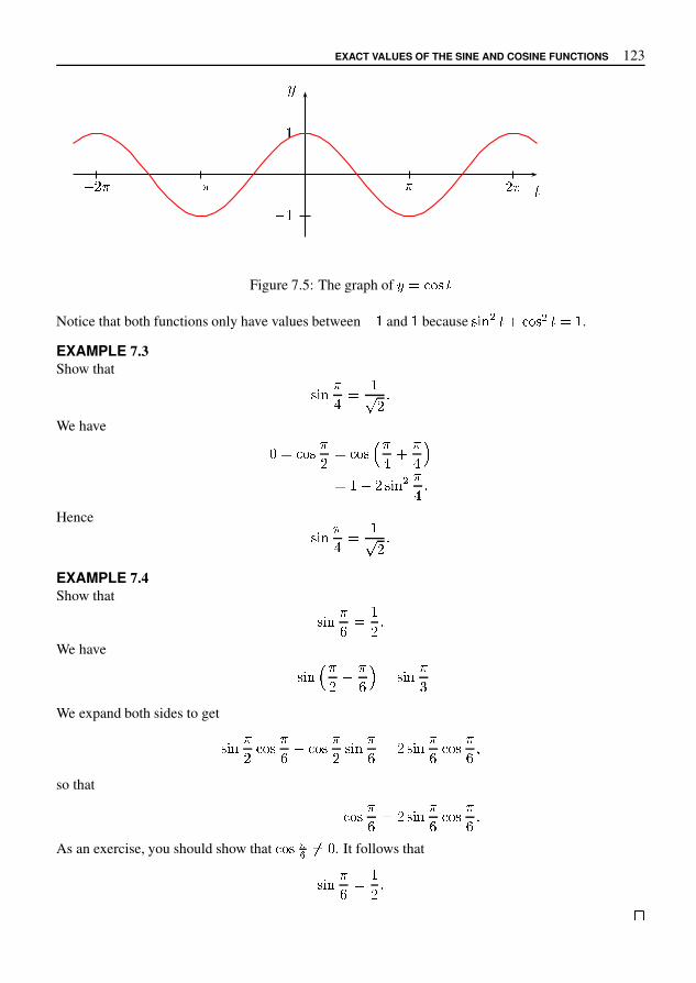
EXACT VALUES OF THE SINE AND COSINE FUNCTIONS 123
�
� �
�
��� � � �� � �
Figure 7.5: The graph of � � � �Notice that both functions only have values between � � and � because � � � � � � � � � � � � .
EXAMPLE 7.3Show that
� � � �� � �
� � �We have
� � � �� � � � #
�� � �
� $� � � � � � � � �
� �Hence
� � � �� � �
� � �EXAMPLE 7.4Show that
� � � �( � �
� �We have
� � � #�
� � �( $ � � � � �
)We expand both sides to get
� � � �� � � �
( � � � �� � � � �
( � � � � � �( � � �
( ,so that
� � �( � � � � � �
( � � �( �
As an exercise, you should show that � � � - .� . It follows that
� � � �( � �
� �/

124 TRIGONOMETRIC FUNCTIONS
� � ��
��
��
��
� ��
� ��
� �� �
� � � 0�
��
� �� �
� 1� �
��
� ��
� 0
� � � 1� �
��
� ��
� 0 � �� � �
� � � � �� � �
Table 7.1: Exact values of the sine and cosine functions
Table 7.1 summarises important exact values for the sine and cosine functions. Further exact valuescan be found using the periodicity of these functions or properties such as � � � � � � � � � � and
� � � � � � � � � � � .All of the results of this section have been derived purely from the power series definitions of the
functions and these power series were obtained from the differential equation. We have not madeuse of the definitions of the trigonometric functions as ratios of sides of right-angled triangles. Theimportance of these functions in calculus is their relation to oscillation problems, rather than theirrelation to triangles.
EXERCISES 7.5
Use the results � � � � � , � � � � � , � � � ( � � � and � � � ( � � � , together with the additionformulas for sine and cosine to derive the following results.
1. � � � � � � 2. � � � � �3. � � � � � � 4. � � � � � �5. � � .
�� � � 0 � � � � 6. � � .
�� � � 0 � � � �
7. � � � � � � � � � � � � 8. � � � � � � � � � � �9. � � � � � � � � � � � � 10. � � � � � � � � � � � � �
11. � � � � � 5 � � � � � � 12. � � � � � 5 � � � � � �Use the exact values of the sine and cosine functions given in Table 7.1 to derive the results in Ex-ercises 13–20. You may also need to use other properties of these functions, such as the additionformulas.
13. � � � � � � 14. � � � �� � �
15. � � � �� � � � 16. � � � �
� � �� �
17. � � 8 �� � �
� � 18. � � 8 �� � � �
�19. � � � � �
� � � 20. � � �� � � �
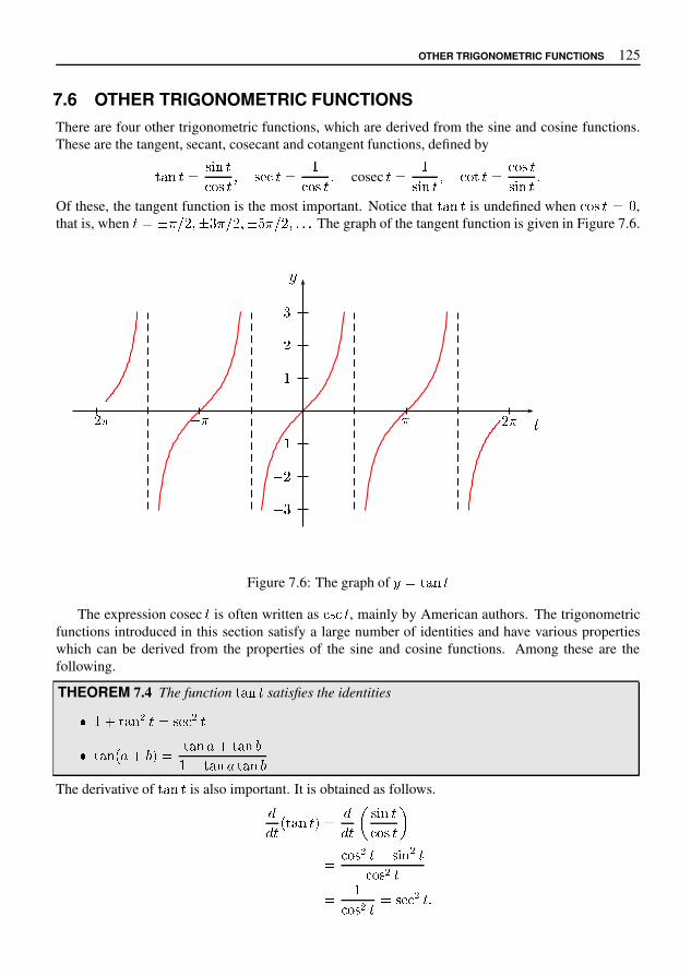
OTHER TRIGONOMETRIC FUNCTIONS 125
7.6 OTHER TRIGONOMETRIC FUNCTIONSThere are four other trigonometric functions, which are derived from the sine and cosine functions.These are the tangent, secant, cosecant and cotangent functions, defined by
� � � � � � � � � � � � � � � � � � � � � cosec � � �� � � � � � � � � � �� � � �Of these, the tangent function is the most important. Notice that � � � � is undefined when � � � � � ,that is, when � � � � � � � � � � � � � " � � � � � � � The graph of the tangent function is given in Figure 7.6.
��
$ �$ �$
(
)� � �$ �$ � �
Figure 7.6: The graph of * � � � � �The expression cosec � is often written as � � , mainly by American authors. The trigonometric
functions introduced in this section satisfy a large number of identities and have various propertieswhich can be derived from the properties of the sine and cosine functions. Among these are thefollowing.
THEOREM 7.4 The function � � � � satisfies the identities
. � 0 � � � 1 � � � � 1 �.
� � � 4 6 0 8 9 � � � � 6 0 � � � 8� $ � � � 6 � � � 8The derivative of � � � � is also important. It is obtained as follows.
:: � 4 � � � � 9 � :: � < � � � � � � >� � � 1 � 0 � � 1 � � � 1 �� � � � 1 � � � � 1 � �
126 TRIGONOMETRIC FUNCTIONS
EXERCISES 7.6
1. Derive the identity � � � � � � � � � � �2. Show that
� � � � � � � � � � � � � � � � �� � � � � � � � � �In the following three exercises, derive the given expressions for the derivatives of � � � , cosec � and � � � .
3.!! � � � � � � � � � � � � � 4.
!! � � cosec � � � cosec � � � �5.
!! � � � � � � � cosec � �In Exercises 6–9, find the derivative of the given function.
6. ' � � � � � 7. ' � � � � � * � + �8. ' ./ cosec 0 � 9. ' � cosec � �
10. Suppose you are told that the function
1 � � � 456
� * � �� 7 � : ;� 7 � ;is continuous at � ; . Let = � > @ be a sequence converging to 0. Assuming that the statementabout the continuity of 1 at � ; is correct, what does the sequence
A � * � � >� > Bconverge to? Test your answer by taking some specific examples for = � > @ .
11. Let = � > @ be any sequence converging to 0. Show that the sequence
A � * � � >� > Bconverges to 1. Hence show that the function 1 in the previous example is continuous.

CHAPTER 8OSCILLATION PROBLEMS
8.1 SECOND ORDER LINEAR DIFFERENTIAL EQUATIONSThe differential equation obtained for the oscillations of a stretched string occurs in almost all oscilla-tion problems, whether these involve vibrating strings, automotive suspensions or electric circuits. Wewill analyse the equation using the example of a body of mass
�hanging on a spring (Figure 8.1).
�
� �� �
�
�
�Equilibrium
position
Figure 8.1: A weight on a spring
Let � be the unstretched length of the spring and let � be the distance from the suspension point.Newton’s second law of motion tells us that
� � � �� � �
�
where
is the total force on the body. There are a number of contributions to the total force. Thereis the force
� due to gravity which pulls the mass down. It is given by � � � �
where � is the acceleration of gravity. Next there is the force �
in the spring itself. If the mass ispulled down the spring pulls it up, while if the mass is pushed up the spring pushes it back down.Hooke’s law states that the spring force is proportional to the extension of the spring, so that
� � � � � � � � �
128 OSCILLATION PROBLEMS
where � is a positive constant. The body may experience frictional or damping forces due to air,immersion in a liquid or having a dashpot or shock absorber attached. Such forces are usually pro-portional to the velocity, but act in the opposite direction. The frictional force can written in theform � � � � � � �� where � is a positive constant. Finally there may be an external time-dependent driving force whichcan be of any form. We denote it by
� � � . The total force acting on the mass is
� � � � � � � � � � � � � �and so the differential equation is
� � � �� � � � � � � � � � � � � � �� � � � � � (8.1)
We will do a little work on this equation before attempting to solve it. First rewrite it as
� � �� � � �� � � � � � �� � �� � �� � � � �� � (8.2)
Next, put
! � � � � � �� �We do this in order to simplify the later mathematics, but there is also a physical interpretation of !which comes about as follows. If there is no external force and the particle is hanging at rest, then� $ � � � ' , � $ $ � � � ' and equation (8.1) gives us
� � � � �� �This is the equilibrium position, so ! is the displacement from equilibrium. In order to substitute theexpression for ! into equation (8.2) we need the derivatives of ! in terms of the derivatives of � . Theseare
� !� � �� � � � � � �� � � �� � � !� � � � � �� � �
Using these results and putting � * � � � , � * � � - � and� � � * � � � � � enables us to write
equation (8.2) as ! $ $ � - � ! $ � � ! � � � � � (8.3)
This is the basic differential equation for forced damped oscillations. It is a second order equation andwe shall find solutions in terms of exponential and trigonometric functions. The equation is said tobe linear because it contains only a sum of first powers of derivatives. More precisely, a second orderlinear differential equation is one of the form
0 � � ! $ $ � 2 � � ! $ � � � � ! � � � � �
SECOND ORDER LINEAR DIFFERENTIAL EQUATIONS 129
The function � � � � is not identically zero, but otherwise � , � and � can be arbitrary functions of � . Inthis book we will only consider the case where � , � and � are all constants with � � . If the right handside of a linear differential equation is identically zero, then the equation is said to be homogeneous,otherwise it is non-homogeneous. In the spring problem analysed above, the equation is homogeneousif there is no driving force.
EXAMPLE 8.1� The equation � � � � � � � � � � � is homogeneous and linear.
� The equation � � � � � � � � � " � is non-homogeneous and linear.
8.1.1 The homogeneous case
We begin with a general linear homogeneous second order differential equation of the form
� � � � � � � � � � � � ' (8.4)
where � � , � and � are constants. To get solutions of this equation we generalise from the first ordercase. If � � � � � � � , then
� � � � �� �
and the solution is� � � , - � �
� . 'which is of the form � � � , / �
. In particular, if � � 2 , then the solution is of the form � � , / �.
This suggests we try exponential functions of this form as trial solutions in the second order case. Put� � , / �
in equation (8.4) to get
� 4 5 , / �� � 4 , / �
� � , / �� 7
Hence� � 4 5 � � 4 � � � , / �
� and, since , / �
is never zero, we have
� 4 5 � � 4 � � � 7This quadratic equation is called the auxiliary equation of the original differential equation (8.4). Notethat powers of 4 in the auxiliary equation correspond to orders of differentiation in the differentialequation. In particular, � is the zeroth derivative and is replaced by 1. If , / �
is to be a solution of thedifferential equation, then the constant 4 has to satisfy the auxiliary equation.
EXAMPLE 8.2Use the method above to find two solutions of the differential equation
� � � � � � � � � � � 7Solution. Substitute � � , / �
into the differential equation. Then
4 5 , / �� � 4 , / �
� � , / ��
� 4 5 � � 4 � � � , / ��
4 5 � � 4 � � � � 4 � 2 � � 4 � � � � '

130 OSCILLATION PROBLEMS
and � � � � or � � � . Thus both � � � �and � � � � �
are solutions of the differentialequation. We can check this by direct substitution. If we put � � �
, then
� �� � � � � � � � � �
� � � � � � � � � � � � � � � � � � �
� " $so that � � �
is a solution. Similarly, � � � �is also a solution. More interesting, if we
put ' � ( � � � ) � � �for any constants
(and
), then we find ' is also a solution. This is
straightforward to check. *Let + � and + � be any functions. If
(and
)are constants, we call
( + � � ) + � a linear combinationof + � and + � . In the example above, a linear combination of two solutions to the differential equationwas also a solution. This is a consequence of a general result known as the principle of superposition .
THEOREM 8.1 The principle of superpositionLet � and � be any two solutions of the linear homogeneous equation
, � � � � � � - �
� � � � � " $
where , , - and � are constants with , 0� " . Then any linear combination( � � ) � of � and � is
also a solution of the differential equation.
This theorem can be proved by using substitution to check that( � � ) � satisfies the differential
equation.We will need another result from the theory of differential equations. We shall assume this result
without proof.
THEOREM 8.2 For any second order linear homogeneous differential equation, we can find twosolutions which are not constant multiples of each other. If these solutions are � and � , then everysolution has the form
( � � ) � for arbitrary constants(
and)
.
As in the first order case (page 103), a solution of a differential equation containing arbitraryconstants, with the property that every solution of the equation can be obtained by taking particularvalues for the constants, is called the general solution .
We have shown how to use the auxiliary equation to find solutions to a particular linear homogeneousdifferential equation with constant coefficients. However, an arbitrary linear homogeneous differentialequation will have solutions belonging to one of three classes of functions, depending on the natureof the solutions of the auxiliary equation.
Case 1: Distinct roots of the auxiliary equation
This is the easiest case to deal with. Suppose the roots � � and � � are real and different. Then 1 � �
and 1�
�are both solutions of the differential equation and the general solution is
� ( 1 � � � ) 1�
� $where
(and
)are arbitrary constants.
SECOND ORDER LINEAR DIFFERENTIAL EQUATIONS 131
EXAMPLE 8.3Solve the equation
� � � � � � � � � � � � � � � � � � � � �The first step is to find the auxiliary equation. In the above differential equation, we replace � � � � � � by
� � , � � � � � by � and � � � � by � . This gives
� � � � � � � � �The roots are � � � ! and � � " . The solution to the differential equation can now be written downas
� � $ % & ' � ( % ) � �EXAMPLE 8.4Solve the equation
* � � � + * � � - * � � �The auxiliary equation is � � � + � � - � � and its roots are � � and 6, so the general solution of
* � � � + * � � - * � � is* � $ % & � ( % 5 � �
EXAMPLE 8.5Solve the initial value problem
� � � � � � � � � � � � � � � � � � � � 6 � � � � � � � 6 � � � � � � �As in Example 8.3, we find the general solution to be
� � $ % & ' � ( % ) �
(8.5)
and we have to use the initial conditions to find$
and(
. In equation (8.5), put � � � and � � � . Thisgives � � $ ( �
Next, differentiate (8.5) to get
� � � � ! $ % & ' � " ( % ) � �Put � � � � and � � � to get � � � ! $ " ( � We now have two equations in
$and
(:
$ ( � �� ! $ " ( � �
which we solve to get$ � � BC and
( � BC . The final solution is
� � �E � % ) � � % & ' � � �
Note that a differential equation has many solutions. These may all be written in one form as thegeneral solution. A differential equation together with initial conditions has just one solution, inwhich the arbitrary constants in the general solution have been given particular values.

132 OSCILLATION PROBLEMS
EXAMPLE 8.6Solve the equation
� � � � � � � � � � � � � � � � � � � � � �This is a third order differential equation, but it is linear, homogeneous and has constant coefficients.The first step is still to find the auxiliary equation. In the above equation, we replace � � � � � � � by � � ,
� � � � � by � and � � � � by � . This gives
� � � � � � � � �The roots are now a bit harder to find. One way is to try various values for � such as � �
� � ! � � ! % � � � � and see if we can get lucky. Once we find one root, we can do a long division andend up with a quadratic, which we can solve. For the above auxiliary equation, we find � � � is asolution. This is done by long division of � � � � � � by � � . We have
� � � � � � � � � � � � � - � � � �� � � � � � � % � � � � 1 � �
The roots are � � � , � � % and � � 1 . The solution to the differential equation can now bewritten down as
� � 6 7 � � 8 7 - � � 9 7 : � � �
Case 2: Equal roots of the auxiliary equation
Suppose the auxiliary equation has a repeated root � ; . Then < ; � 6 7 > � �is one solution and in
order to get the general solution we need a second independent solution. We can do this by using themethod of variation of parameters introduced in Chapter 6 on page 104.
We try a solution < � @ � � � 7 > � �, where we replace the constant
6in the first solution by a function
@ . Then
< � � @ � 7 > � � � @ � ; 7 > � �
< � � � @ � � 7 > � � � % @ � � ; 7 > � � � � -; @ 7 > � �
Substitution in the differential equation E < � � � F < � � � < � � and cancellation of the exponential gives
E � @ � � � % @ � � ; � � -; @ � � F � @ � � @ � ; � � � @ � � �A rearrangement of this equation yields
@ � E � -; � F � ; � � � � @ � � F � % � ; E � � E @ � � � � � (8.6)
Now we use the fact that � ; is a repeated root of the auxiliary equation E � - � F � � � � � . Thisimplies two results:
O Firstly, E � -; � F � ; � � � � .
O Secondly, E � - � F � � � � E � � � ; � - � E � � - % � ; � � � -; � . Equating coefficients inthis equation gives F � % E � ; .

SECOND ORDER LINEAR DIFFERENTIAL EQUATIONS 133
Using the results � � �� � � � � � � � and � � � � � � in equation (8.6) enables us to deducethat � � � � � . Since � � � is an assumption made at the outset, we conclude that � � � � , so that
� � " $ � % for arbitrary constants$
and%
. Thus a second solution to the differential equation is
& � � " ( ) � � � $ � % " ( ) � � +This is, in fact, the general solution since the two solutions ( ) � �
(the case% � ,
$ . ) and ( ) � �
(the case% . ,
$ � ) are not constant multiples of each other.Historically, a good deal of trial and error was used in discovering methods for solving particular
types of differential equations. In the present case for example, there is no prior guarantee that replac-ing a constant by a function will produce a second solution. However, as we have just shown, it does.Once this rule for the second solution has been found, it is easy to apply.
EXAMPLE 8.7Let / & � � � 1 & � � & � . The auxiliary equation is / � � � 1 � � . � with roots � � . 7 8 : � . 7 8 .The general solution of the differential equation is
& < ( = �� > � $ ( = �
� > +
Case 3: No real roots of the auxiliary equation
An example of this case is the equation & � � � � & � � � & � . The auxiliary equation is � � � � � � � � which has no real roots. However, it is easily checked that both ( � C D E and ( � G I C satisfy thedifferential equation. This raises two issues:
K How would we find the solutions ( � C D E and ( � G I C if they were not known?
K The auxiliary equation arose by considering exponential functions as trial solutions. What isthe connection between these and the trigonometric functions?
We will address these and other matters in the following sections.
EXERCISES 8.1
In Exercises 1–8, state whether the equation is linear or nonlinear. If the equation is nonlinear, give areason.
1. L � � � " � � L � � " � L � " G I C 2. & � � � L " � P & � L " & � � L " � & � L " �3. 8 & � � � P & � � & � 4. � � � � " P T � 8 �5. & � � � & � � & � � 6. & � � � � " � P & � � � " � > & � " 8 7. � L � � � L " � 8 8. L � � " � 8 L � " .
Solve the following differential equations. Where initial conditions are given, find the particularsolution satisfying the initial conditions. Otherwise, find the general solution.
9. & � � � 8 & � � � & � 10. & � � � V & � �11. & � � � � & � � & � 12. & � � � P & � � P & �13. & � � � � & � � 8 & � 14. & � � � & � � 8 & �15. & � � � 8 & � � : & � � " 8 : & � � � " 1

134 OSCILLATION PROBLEMS
16. � � � � � � � � � � � � � � � � � � � � � � � � � �
17. � � � � � � � � � � � � � 18. � � � � � � � � ! � � �
19. � � � � � � � ! � � � 20. ! � � � � ! � � � � � �
21. ! � � � � � ! � � � � � � � � 22. � � � � � $ � � � � � � � � % � � �
23. % � � � � � � � � ! � � � 24. � � � � � � � � � � �
25. � � � � � � � � � ! � � � � � � � 26. � � � � � � � � � � � � � � �
27. � � � � � % � � � � 28. � � � � � � � � � � � � � � � � � �
29. � � � � � � � � � � 30. � � � � � � � � � � � � �
31. � � � � � � � � � � 32. ' � � � ) ' � � ! ' � �
33. � � � � � � � � � � � � 34. ! ' � � � � ' � � $ ' � �
35. � � � � $ � � � � � � � 36. � � � � � � � � % � � �
37. � � � � $ � � � � � � � 38. � � � � � � � � � � �
39. ! � � � � ! � � � � � � 40. � - � � � � � - � � ) - � �
8.2 COMPLEX NUMBERSIn order to deal with the case where the auxiliary equation has no real roots, we have to considercomplex numbers. It is often stated that complex numbers were introduced in order to solve quadraticequations such as ' . � � � � , but this is historically inaccurate. Mathematicians were quite happyto accept that such an equation had no real roots and there was no compelling reason to consider anyother possibilities. For reasons which we shall not detail here, the need for complex numbers wasfirst encountered in the sixteenth century in connection with cubic equations. A formula for solvingsuch equations was published by Gerolamo Cardano in 1545 in Italy and this formula often requirescomplex numbers as part of the work in reaching the answer, even if all the roots of the equation arereal. It was the attempts to understand this aspect of the formula which provided the initial impetusfor the study of complex numbers.
�
'
�
Im � � �
Re � � � �
Figure 8.2: The complex number �

COMPLEX NUMBERS 135
The new idea that occurs with regard to complex numbers is that we go from the usual numberline to a number plane, that is, we consider pairs of real numbers. We can then think of a complexnumber as a point in the plane.
Let us now be more precise. A complex number is an ordered pair of real numbers. For example� � � � , � � � � and � � � � (with � � � � � ) are all complex numbers. Complex numbers are often denotedby the symbols � or � . If � � � � � � is a complex number, then � is called its real part and is denotedRe � � . The imaginary part of � is � and is written Im � � . Two complex numbers � � and �
�are equal
if Re � � � � Re � �
� and Im � � � � Im � �
� . Complex numbers can be represented by points in the
plane and when the plane is used for this purpose, it is called an Argand diagram or complex plane(Figure 8.2).
In order to do anything useful with complex numbers, we have to be able to add, subtract, multiplyand divide them. The rules for addition and subtraction are straightforward. We add (or subtract, asthe case may be) the corresponding real and imaginary parts of the two complex numbers. Thus if
� � � � � � � � � and �
�� � �
�� �
� , then
� � � �
�� � � � � �
�� � � � �
� �
� � " �
�� � � � " �
�� � � " �
� $
EXAMPLE 8.8If � � � � � � and � � � ) � " - , then
� � � � � � � � � � ) � " -
� � � � ) � � � � " -
� � � � " ) $
2
There is also a simple rule for multiplying complex numbers by real numbers. If � � � � � � is acomplex number and 5 is any real number, then we define 5 � by
5 � � � 5 � � 5 � �
so for example if � � � � � " � , then � � � � � ) � " � .The rule for multiplying two complex numbers is more complicated, but the reasons for it will
become clear soon enough. If � � � � � � � � � and �
�� � �
�� �
� , then we define
� � �
�� � � � �
�" � � �
�� � � �
�� �
�� � $ (8.7)
EXAMPLE 8.9If � � � � � ) and � � � � � ; , then
� � � � � � ) = � � � ;
� � � = � " ) = ; � � = ; � ) = �
� � � � ) ; $
2
136 OSCILLATION PROBLEMS
There are some interesting consequences of these arithmetical rules. Firstly, the complex numbers ofthe form � � � � behave like ordinary real numbers. We identify the complex number � � � � with thereal number � . For example � � � � � � � � � � � � is equivalent to the statement � � � and
� � � � � � � � � ! � � is equivalent to # � � ! . Thus in the Argand plane, the real numbers lie alongthe ' axis with the point � � � � corresponding to the real number � . In particular, we write � ) � � � ) .
Now for the amazing bit of magic that gives the whole system its remarkable properties. If wesquare the complex number � � � ) we get
� � � ) � � � ) � � � # � 3 ) # ) � � # ) ) # � � � 3 ) � � � (8.8)
which we can identify as the number 3 ) . Thus in the complex number system, the number 3 ) or,more precisely, the number � 3 ) � � , has a square root, namely � � � ) . We can write this fact as
� � � ) 9 � 3 ) : (8.9)
Notice that the square root � � � ) of 3 ) is not a real number. If, as is commonly done, we write �
for the complex number � � � ) , then equation (8.9) becomes the mysterious looking result
� 9 � 3 ) :
Once we can find ; 3 ) , then we can also find the square root of any negative number. For instance; 3 = � > � = � 3 ) � � .
The approach to complex numbers that we have used is logically sound. There is nothing mys-terious about them. Complex numbers are simply ordered pairs of real numbers with certain rulesof arithmetic. They can be represented on diagrams and visualised in a concrete manner. This wasnot always the way in which they were discussed. Historically, complex numbers were introduced bysimply defining � to be a number having the property � 9 � 3 ) . Since no real number has this property,
The imaginary numbers are a wonder-ful flight of God’s spirit. They are al-most an amphibian between being andnot being. Gottfried Leibniz
there are severe logical difficulties with this approach. It wasnot until the ordered pair definition was thought of that com-plex numbers were put on a firm logical base. The first per-son to think of this idea appears to have been Kaspar Wessel,a Norwegian surveyor, in 1797, but his work went unnoticed.In 1806, Jean Argand published an account of the graphicalrepresentation of complex numbers. Initially this also went un-noticed, but by the end of the second decade of the nineteenth century the idea had become familiarto mathematicians.
8.2.1 The number �
Writing � for the complex number � � � ) gives us an alternative notation for complex numbers. If� � � ' � B is any complex number, we can write
� � � ' � B � � ' � � � � � B � ' � ) � � B � � � ) � ' � B :
This notation is almost always used in preference to the ordered pair notation because it is moreconvenient for computational purposes. If we write complex numbers in the form ' � B , we can use

COMPLEX NUMBERS 137
all the normal rules of algebra, with the additional rule that � � � � � . So for example, if � � � � � � �and �
��
� � �
�, then
� � ��
� � � � � � � � �
� ��
�
� � �
� � � � ��
� � ��
� �
� �� �
�� � � �
� � � � �
�
�� � � (8.10)
If we write this last statement in the ordered pair notation, we have
� � ��
� � � �
� � � ��
� � ��
�
� � � �
which is just the rule for multiplication we gave in equation (8.7). Historically, the result (8.10) camefirst, but from a logical point of view it needs to come second. From now on we shall use the � �form of notation.1
So far, we have not dealt with the matter of division of complex numbers. This is best handled bythe notation of this section. We have
� � � � �
�� � � � � � � � � �
� � � � � � � � �
�� � � � � � � � � �
� � � � � �
�� � �
� � � � � � � �
� � �'
This process is called realising the denominator.
EXAMPLE 8.10Find all the roots of the equation � � � * .Solution. We use the usual quadratic formula:
�� � - . � � � / � �
0 �
with � � � � � � � . This yields
�� � - . � � /
0� �
�� � � - � . 7 � '
8
It is not clear that this example achieves anything useful. Indeed, if complex numbers had nevergot beyond this stage, they would have been abandoned a long time ago. We will soon show that wecan do far more with complex numbers than simply write down solutions of polynomial equations.
8.2.2 Terminology
Let � � � � be a given complex number. Plot � in the complex plane (Figure 8.3). We join � , thatis, the point � � � � , to the origin by a straight line making an angle
with the positive direction of the
axis. Let the length of this line be ; .
1Sometimes the symbol is used instead of � , especially in electrical and electromagnetic applications. This is to avoidconfusion with the use of � for electric current.

138 OSCILLATION PROBLEMS
�
��
�
�
�
�
�
�
Figure 8.3: The conjugate, modulus and argument of a complex number
The following terminology is used.
� The modulus or amplitude of � is the length � . We write it as � � � . By Pythagoras’ theorem
� � � � � � �
� The argument or phase of � is the angle�. We write
� � � � � � � or� � Ph � � � . We take
�
to be positive if it is measured counter-clockwise from the direction of the positive � axis andnegative if it is measured clockwise from the direction of the positive � axis. Its value lies inthe interval � � � � � � .
� From simple trigonometry (Section 7.4.1), we have � � � � " �and � � � " ' ( �
. Thus � �� � � " � � � " ' ( � � . This is often abbreviated to � � � cis
�. Either of the two expressions
� � � " � � � " ' ( � � or � cis�
is called the polar form of � . We call � � � � the Cartesian form of � .
� The complex conjugate of � is the complex number�� � � 0 � � . When drawn in the complex
plane it is the reflection of � in the � axis. Notice that if � is real then�� � � .
EXAMPLE 8.11If � 2 and � are any complex numbers, show that
� � 2 � � � �� 2 � �� � � 2 � � �� 2
�� � �� 2 � 2 � � � 2 �
COMPLEX NUMBERS 139
Solution. We put � � � � � � � � � and � � � � � � � � � , so that�� � � � � � � � and
�� � � � � � � � . Then
� � � � � � � � � � � � � � � � � � � � � � � � � � � � � � � � � � � � � � � � � � � � � � � � � � � � � � � � � � � � � � � �� � � �� � �
Next we have
� � � � � � � � � � � � � � � � � � � � � � � � � � � � � � � � � � � � � � � � � � � � � � � � � � � � � � � � � � � � � � � � � � � � � � � � � � �� � �� � �
Finally�� � � � � � � � � � � � � � � � � �
� � � � � � ��� � � � � � �There is a useful fact about complex roots of polynomial functions which we shall need later. Thisis that complex roots always occur in conjugate pairs if the coefficients in the polynomial are real.Suppose for example that � � is a zero of the polynomial � � � � � � � , where � , � and are real. Then� � �� � � � � � � # . Consequently
� � �� � � � � � � �# %that is,
� �� �� � � �� � � � # �Thus
�� � is also a zero of the polynomial.
EXAMPLE 8.12The Cartesian form of & cis
' ( ) is given by
� � � � � & + , - / + 01 2 � � / 5 6 + 0
1 2 2� 8 8 : 1 �
EXAMPLE 8.13Find the polar form of � � < � .Solution. We have � � � � > < � � � < � � : @ �We also have , - / � � < C : @ % / 5 6 � � < C : @ %so
� � F 0 C 8 and � � : @ cis � F 0 C 8 .
140 OSCILLATION PROBLEMS
EXERCISES 8.2
Let � � � � � � , � � � � � and � � � � � � . Evaluate each of the real or complex numbers inExercises 1–21. Where a number is complex, express it in the form � � � � .
1. Re � � 2. Im � � 3. � � � � �4. � � � � 5. � � � � � 6. Im � � � � � �7. � � � � � � � 8. � � � � � � � � � 9. � � � � � �
10. � � � � � � � � 11. � � � � � �� 12. � � � � � � � �13. � � � � � � � � � 14. � �� � � � � � � 15. � � � �16. Re � � �� � � 17.
� � � � 18.
� � � � �� � � �19.
� �� � � � �� � 20.� �� � � � 21. ����
� �� � � � ����In Exercises 22–27, express the given complex numbers in polar form.
22. � � � � � 23. � � � 24. " � " �25. � � � � � 26. � � 27. � � �
Solve the equations:
28. � � � � � " � ) 29. � � � � � � � ) 30. � � � � )31. � � � � ) 32. � - � � ) 33. � - � � � � � )
8.3 COMPLEX SERIESLet us take an infinite sum of the form .�
� / �� � 1
where � � is a complex number for each 2 � 1 � 1 1 ; ; ; If we put � � � � � � � � � for 2 � 1 � 1 1 ; ; ; ,then we can write .�
� / �� � � .�
� / �� � � �
.�� / �
� � ;We say that the complex series � .� / � � � converges if each of the real sums � .� / � � � and � .� / � � �
converges. If = � � .� / � � � and > � � .� / � � � , then we can write
.�� / �
� � � = � � >for the sum of the complex series.
COMPLEX SERIES 141
8.3.1 The complex exponential
We have previously defined � � for all real numbers � by letting
� � � � � � � � � �� � � � � � �� � � � �
In a similar way, define � � for all complex numbers � by letting
� � � � � � � � � �� � � � � ��
� � � � �The ratio test applies to complex series as well as real series. Using this test, we can show that theseries for � � converges for any complex number � . For a given complex number � , this series is hardto sum as it stands, but if we rewrite it we can make things simpler. Consider first the case where
� � � � with � " . Then
� � � � � � $ � � % � � $ � � % �� � $ � � % () � � � � $ � � % �� � � � �
� � � � - � � � - �� �� � � () � � � �
� 0 � - � � � � () � � � � 3 � 0 � - � �� � � 56 � � � � 3� 8 : < � � < > ? � AWe have shown that � � � 8 : < � � < > ? � (8.11)
for any real number � . This is a surprising and remarkable result. For real functions there seems to beno connection between the exponential function and the sine and cosine functions. Yet here we have aconnection between these three functions and the square root of - � . All very strange. Equation (8.11)was discovered by Leonhard Euler in the eighteenth century and is known as Euler’s formula . Thenotation � stands for Euler’s number. From Euler’s formula we have
� B � � 8 : < $ - � % � < > ? $ - � % Fso that � B � � 8 : < � - � < > ? � (8.12)
If we add equations (8.11) and (8.12) and solve for 8 : < � , we find
8 : < � � � � � B �
ASimilarly, if we find the difference of equations (8.11) and (8.12) and solve for < > ? � , we find
< > ? � � � � - � B �
�A
Euler’s equation gives rise to yet another remarkable identity. If we put � � J we get
� � � � - � A
142 OSCILLATION PROBLEMS
Here we have four of the most important numbers in mathematics connected by one very simpleequation.
We showed earlier that � � � � � � � � � for any real numbers � and � . It can be shown that the sameidentity holds for complex exponents � and � , so that � � � � � � � � � . In particular, we have
� � � � � �
� � � �� � � � � � � � � � � � � (8.13)
EXAMPLE 8.14If � � # cis
�, then
� � # � � � ��
� � � ��
�� # � �
If � & � # & � � � and � ' � # ' � �� , then
� & � ' � # & # ' � � � � � �� �
So to multiply two complex numbers, we multiply their moduli and add their arguments.
EXAMPLE 8.15If � � ) � + , - , then
� ' � � � . � � ' � � � � + , - � � � � � + , - �
�� '
)� 1 � 3 - �
5
As a consequence of Euler’s formula (equation (8.11)) multiplication of complex exponentialfunctions is intimately connected with addition formulas for trigonometric functions.
� � � � �� � � � � � � & � � � � � & � � � � � � ' � � � � � ' �
� � � � � & � � � � ' 7 � � � � & � � � � ' � � � � � � & � � � � ' � � � � � & � � � � ' �� � � � � � & � � ' � � � � � � � & � � ' �
� � � � � � �� �
If we take � & � � ' ��
in this result, then we see that
� � � � ' � � ' �
so that
� � � ��
� � � ��
� ' � � � � � )�
� � � � )�
�
More generally, we can use the equation
� � � � @ � � @ �
to show that� � � �
�� � � �
�� @ � � � � � A
�� � � � A
��
This last result is known as de Moivre’s Theorem.

COMPLEX ROOTS OF THE AUXILIARY EQUATION 143
EXAMPLE 8.16Use de Moivre’s Theorem to show that
� � � � � � � � � � � � � � � � � � � � �� � � � � � � � � � � � � � � � � � � � �
Solution. We have
� � � � � � � � � � � � � � � � � � � � � � � � � � � � � � � � � � � � � � � � � � � � � � � � � � � � � � � � � � � � �� � � � � � � � � � � � � � � � � � � � � � � � � � � � � � � � � � �
If we equate the real part of the left hand side to the real part of the right hand side we get
� � � � � � � � � � � � � � � � � � � � � �while equating the imaginary parts of both sides gives
� � � � � � � � � � � � � � � � � � � � ��
Notice the way in which complex numbers have been used as tools in obtaining results which arepurely real.
EXERCISES 8.3
1. If � � " � � , evaluate # " � # .2. If � � � � � � � � � � � �
, show that
$ � � � � � � � $ � + � � � � � � � � � � � � � � � � �
3. Use de Moivre’s theorem to show that
� � � . � � + � � � 0 . � 3 4 � � � 5 . � $ 4 � � � � . � $
4. Prove that the solutions of � 5 � � � � � $ � ; are given by + � � � � = > ? @ � and + � � � � > � = > ? @ � for= � $ � +
8.4 COMPLEX ROOTS OF THE AUXILIARY EQUATIONWe can now return to the differential equation
C D E E � F D E � D � ; (8.14)
in the case where the auxiliary equation C I � � F I � � ; has complex roots. We are assuming thecoefficients C , F and are real so that the roots occur in conjugate pairs. Let J L �
�be the roots of
the auxiliary equation. Then the general solution to the differential equation (8.14) can be written incomplex form as
D � M " � � N � � � � � O " � � P � � � � �

144 OSCILLATION PROBLEMS
where�
and�
are arbitrary constants. This form of the solution is not particularly useful for ourneeds, since we want real solutions. However, we can rewrite it in real form using the results of theprevious section. We have
� � � � � � � � � � � � � � � � � � � �� � � � � � � � � � � � � � � � � �� � � � � � � � � � � � � � � � �� � � � � � � � � � � � � � � � � � � � � � � � � � � � � � � �� � � � � � � � � � � � � � � � � � � � � � � � �� � � � � � � � � � ! � � � � � � � "
where� � � � �
and! � � � � � � � . The constants
�and
!are real if
�and
�are suitably
chosen complex numbers. We have come to an important result.
THEOREM 8.3Suppose # % �
are the roots of the auxiliary equation of the homogeneous linear equation
& � ' ' � ) � ' � � � � + "where & , ) and � are constants. Then the general solution of this differential equation is
� � � � � � � � � � � ! � � � � � � � -Once again, we have used complex numbers as a tool to obtain a real result.
EXAMPLE 8.17. Solve the equation/ ' ' � � � � 2 / ' � � � � 4 6 / � � � � + -
The first step is to find the auxiliary equation. In the above equation, we replace / ' ' � � � by : ; ,/ ' � � � by : and / � � � by 4 . (Section 8.1.1 in the text justifies this procedure.) This gives
: ; � 2 : � 4 6 � + -The roots are : � � 6 % B � . The solution to the differential equation can now be written downas
/ � � D � � � � � � B � � ! � � � B � � -. Let � ' ' � B � ' � B � � + . The auxiliary equation is : ; � B : � B � + and this has roots : � � 4 % � .
Hence the general solution of the differential equation is
� � � � � � � � � � � ! � � � � � -. The equation � ' ' � B � � N � � + has auxiliary equation : ; � B : � N � + with roots : � � 4 % B � ,
so the general solution of the differential equation is
� � � � � � � � � B � � ! � � � B � � -
SIMPLE HARMONIC MOTION AND DAMPING 145
EXERCISES 8.4
Solve the following differential equations. Where initial conditions are given, find the particularsolution satisfying the initial conditions. Otherwise, find the general solution.
1. � � � � � � � � � � � 2. � � � � � � � � �3. � � � � � � � � 4. � � � � � � � � � � � �5. � � � � � � � � � � � 6. � � � � � � �7. � � � � � � � � � � � 8. � � � � � � � � � � � � � � � � �9. � � � � � � � 10. � � � � � � � � � � �
11. � � � � � � � � � � � 12. � � � � � � �13. � � � � � � � � � � � � 14. � � � � � � � � � � � �15. � � � � � � � � � � " � % � � � � " � % � �16. � � � � � � � � � � � � � " � % � � � � � " � % �17. � � � � � � � � " � % � � � � " � % �
8.5 SIMPLE HARMONIC MOTION AND DAMPINGWe return to the problem of a particle oscillating on a spring. The general oscillation problem requiresthe solution to the differential equation
� � � � � � � � � � � � 1 " 3 % 6At this stage, we have only developed the techniques to solve the homogeneous case
� � � � � � � � � � � � � � (8.15)
where the driving force1 " 3 % � . The exact nature of the solutions of this equation will depend on
the values of the coefficients � and � and we will need to break down the problem into a number ofcases.
Case 1: Simple harmonic motion ( � � )
The simplest case of equation (8.15) occurs when there is no friction. This is the case � � and theequation becomes
� � � � � � � � 6Motion governed by this equation is called simple harmonic motion (SHM). The auxiliary equationis : � � � � � with roots : ; � � and so the solution is
� < = ? @ � 3 � B @ C D � 3 6In order to analyse the motion of the mass, it is convenient to write this equation in the form
� E = ? @ " � 3 � � %

146 OSCILLATION PROBLEMS
for certain constants � � � and � . To do this, we write
� � � � � � � � � � � � � � � � � � �� � � � � � � � � � � � � � � � � � � $
so that
� � � � � � $ � � � � � � � ( (8.16)
Hence
� � * � + � � + $ � � � ��� (
In calculating � , care must be taken to choose the correct quadrant. This can be done by checking thesigns of � � � and � � � � in equation (8.16). Figure 8.4 shows the solution for the case � � 0 , � � 1 2 4 .The constants � and � have direct physical interpretations. The constant � gives the maximum
5
0
� 5
� 0
8
9
: � 0 � � � � 1 2 4 �
1� 1 0 1� 0 1
Figure 8.4: Simple harmonic motion
displacement of the body from the equilibrium position. This distance is called the amplitude of themotion. The constant � is the phase angle. The phase angle determines the initial position of thebody. For instance, if � � � the body starts at the maximum displacement below the equilibriumposition, while if � � 1 the body starts at the maximum displacement above the equilibrium position,since : is positive when the body is below the equilibrium position. The constant � is related to thefrequency2 ? in cycles per second by ? � @ 1 2 � .
EXAMPLE 8.18The motion of a mass on the end of a spring is given by the initial value problem
: A A � : � � $ : � � � � 0 $ : A � � � � � (2The unit of frequency is the Hertz (Hz). A frequency of 1 Hz corresponds to 1 cycle per second.

SIMPLE HARMONIC MOTION AND DAMPING 147
The physical interpretation of this initial value problem is that the mass starts from rest ( � � � � � � )at a distance of 2 units below its equilibrium position ( � � � � � ). According to the discussion above,the solution is
� � � � � � � � � � � � � !Put � � � and � � � in this equation to get
� � � . We now have
� � � � � � � � � � � � � 'so that
� � � ) � � � � � � � � � � � !If we put � � � � and � � � , we find
� � � . The solution is
� � � � � � � !Alternatively, we can write the solution in the form
� � - � � � � � ) � 'so that
� � � ) - � � � � � ) � !We put � � � and � � � in the first equation to get � � - � � � � and put � � � � and � � � in thesecond equation to get � � - � � � � . Hence � � � � � � , so � � � . (We cannot have � � ? , since
� � � � � � A - C � .) The equation � � - � � � � shows that - � � . Thus we end up with
� � � � � � � 'the same solution as before.
Case 2: Weak damping ( � G G )
The roots of the auxiliary equation H I � � H � I � � are
H � KI � ) � M N O I ) O I � ) M N I ) I !
Since � G G , the number N I ) I is nonzero and pure imaginary. Hence the roots of theauxiliary equation form a complex conjugate pair of the form R M � �
and the solution is
� � � S � � � � ��
� � � S � � � � ��
� !EXAMPLE 8.19As an example we take the equation � � � � � � � � W � � � with initial conditions � � � � � , � � � � � � .The roots of the auxiliary equation H I � H � � W � � are H � � ) Z M [ \ Z Z � A � . Hence the solutionis
� � S ^ � � I�
� � � � [ \ Z Z� � � � � � � [ \ Z Z
� � �and using the initial conditions we find
� � � S ^ � � I�
� � � [ \ Z Z� � � Z
[ \ Z Z � � � [ \ Z Z� � � !
This solution is plotted in Figure 8.5.

148 OSCILLATION PROBLEMS
�
�
�
� �
�
�� � �
Figure 8.5: Weak damping
The behaviour shown in this example is typical. The body still oscillates, but the oscillations die awayexponentially. The frequency of the oscillations is changed by the damping.
Case 3: Strong damping ( � � � )
The roots of the auxiliary equation � � � � � � � � � are
� �� � � � � � � � � � � � � � �� � � � � � � � � � �
If � � , the number � � � � � � is nonzero and real. Hence the roots of the auxiliary equation �and � are real and different and the solution is
� " # $ � � � % # $
� �EXAMPLE 8.20Consider the initial value problem
& & � ' & � � � � , � � � � � , & � � � � � �The roots of the auxiliary equation � � ' � � � � are found to be � � � , � � , so the generalsolution is
� " # 9 � � % # 9 : � �Using the initial conditions we get
� ;< # 9 � � �< # 9 : � �The solution is plotted in Figure 8.6.
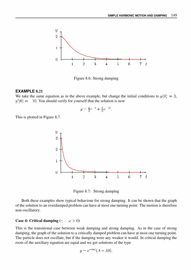
SIMPLE HARMONIC MOTION AND DAMPING 149
� � � � � � ��
�
�
Figure 8.6: Strong damping
EXAMPLE 8.21We take the same equation as in the above example, but change the initial conditions to � � � � � ,� � � � � � � � . You should verify for yourself that the solution is now
� � �� � �
! "� � # �
$This is plotted in Figure 8.7.
� � � � � � ��
�
�
�
Figure 8.7: Strong damping
Both these examples show typical behaviour for strong damping. It can be shown that the graphof the solution to an overdamped problem can have at most one turning point. The motion is thereforenon-oscillatory.
Case 4: Critical damping ( � � � ' � )
This is the transitional case between weak damping and strong damping. As in the case of strongdamping, the graph of the solution to a critically damped problem can have at most one turning point.The particle does not oscillate, but if the damping were any weaker it would. In critical damping theroots of the auxiliary equation are equal and we get solutions of the type
� � � + � , ! - . � $
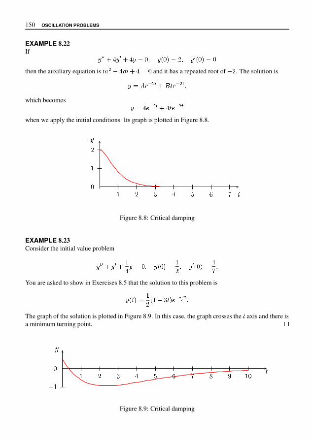
150 OSCILLATION PROBLEMS
EXAMPLE 8.22If
� � � � � � � � � � � � � � � � � � � � � � � then the auxiliary equation is � � � � � � � � and it has a repeated root of � � . The solution is
� � � � � � � � ! � � � � �which becomes
� � � � � � � � � ! � � � �
when we apply the initial conditions. Its graph is plotted in Figure 8.8.
$ � % � & ' (
$
�)
*
Figure 8.8: Critical damping
EXAMPLE 8.23Consider the initial value problem
� � � � � � � $� � � � � � � � $
� � � � � � � �( ,
You are asked to show in Exercises 8.5 that the solution to this problem is
� � ! � � $� � $ � % ! � � � �
� � ,The graph of the solution is plotted in Figure 8.9. In this case, the graph crosses the ! axis and there isa minimum turning point. 2
$ � % � & ' ( 3 4 $
� $
*
)
Figure 8.9: Critical damping
SIMPLE HARMONIC MOTION AND DAMPING 151
As the damping gets weaker ( � � � ) we get closer to simple harmonic motion. As the damping getsstronger ( � � � ), the particle takes longer to return to equilibrium. Infinite damping correspondsto clamping the particle at its initial position. Mathematica is an ideal tool to experiment with thevarious cases.
EXAMPLE 8.24A 5 kg mass is attached to a spring. The mass is pulled down from the equilibrium position andallowed to oscillate. Assume that the motion is undamped and simple harmonic with a frequency
� � � Hz. What is the value of the spring constant � ?Solution. The general equation of motion is equation (8.14) in the text:
� � � � � � � � � � � � � �
where � � � � and � is a proportionality constant for the damping. In this case there is no damping,so � � and the equation is
� � � � � � � � �From � � � � , we have � � � $ � � ' . The spring constant � is given by � � � �
( � � Newtons/metre.
EXAMPLE 8.25A 2 kg mass stretches a spring 2 cm. The mass–spring system is allowed to oscillate in a medium thatimparts a viscous force of 8 N when the speed of the mass is 4 cm/sec. The mass is set in motion fromits equilibrium position with an initial velocity of 8 cm/sec. Determine the initial value problem forthe equation of motion.Solution. The general equation of motion is
� � � � � � � � � � � � � �
so we need to find � and � .If a mass � stretches a spring by a length * , the spring constant � is given by
� + � * �
where + / � ' m/sec � is the acceleration due to gravity. We find � � + � � � � / ' � N/m. Since� � � � , we have � � � / � .
Assuming the resisting force is proportional to the velocity with proportionality constant � , wehave
' � $ � � � � �Hence � � � � N sec/m. We have (on page 147) � � � � , so that � � ; � � . The initial valueproblem for the equation of motion is
� � � � ; � � � � � � / � � � � � @ � B � � � � @ � B � � � ' �

152 OSCILLATION PROBLEMS
EXERCISES 8.5
1. Show that the solution to the initial value problem
� � � � � � � �� � � � � � � � �
� � � � � � � � �� �
is
� � � � � �� � � � ! � � # $ �
� % �
2. A mass of 100 g stretches a spring 5 cm. The mass is set in motion from its equilibrium positionwith a downward velocity of 10 cm/sec. If air resistance is neglected, find the position of themass at any subsequent time � . When does the mass first return to its equilibrium position?
3. A gun barrel weighs 700 kg and the initial velocity of recoil after firing is 25 m/sec. The barrelrecoils against a spring until it stops. A damper is then engaged and the barrel returns to its initialposition without overshoot.
(a) Assume that in the initial phase of recoil, the barrel and spring act like an undamped mass–spring system. What should be the value of the spring constant & so that the barrel travels1.5 m before stopping?
(b) Assume that in the return phase, the barrel and spring act like a critically damped mass–spring system. What should the value of the damping constant � be?
4. The equation of motion of a particle moving in a straight line is
' � � � ) ' � � � ' � �
For what values of the constant ) is the motion oscillatory?
5. The equation of motion of a particle moving in a straight line is
- ' � � � � ' � � ' � �
For what values of the constant - is the motion oscillatory?
6. The motion for an undamped spring–mass system is given by
' � � � � � � � % ' � � � � � ' � � � � � ' � � � � �
Find the equation of motion and sketch its graph for � � � � 5 � 8 .
7. A 20 kg mass is attached to a spring. If the frequency of undamped simple harmonic motion is� 9 : Hertz, what is the value of the spring constant & ?
8. The motion for a damped spring–mass system is given by
' � � � � � � � � ' � � � � � � 8 ' � � � � � ' � � � � � ' � � � � �
Find the equation of motion and sketch its graph for � � ! � � � 5 .

FORCED OSCILLATIONS 153
9. The motion for a damped spring–mass system is given by
� � � � � � � � � � � � � � � � � � � � � � � � � � � � � � � �Find the equation of motion and sketch its graph for � � � � ! � $ .
10. A mass of 5 kg is attached to a spring hanging from a ceiling. When the system is in equilibrium,the spring is stretched 50 cm beyond its natural length . The mass is then pulled down a further10 cm and given an upward velocity of 10 cm/sec. Determine the equation of motion for themass. When does the mass first reach its lowest point after being set in motion?
11. A mass % & oscillates with a frequency of � & when suspended from a spring. The mass % & isremoved and replaced with a second mass % � and the system now oscillates with a frequency� � . Calculate the ratio % & � % � .
12. Give some examples of natural motions that are approximately simple harmonic. Why are exactsimple harmonic motions rare?
13. Give some examples of damping devices in common use.
8.6 FORCED OSCILLATIONSIn this section we consider the case of an oscillatory motion when there is a nonzero driving force.The equation to be solved is
' � � ( � ' � � � ' � + � � � � (8.17)
where+ � � � is not identically zero although it may be zero for particular values of � . We shall only
consider the case of periodic driving forces such as+ � � � � / 1 2 3 5 � or
+ � � � � / 6 8 1 5 � . To solve anequation such as (8.17) there are results about differential equations which tell us that we need to dothree things. We shall simply state these results.
9 We first find the general solution of the homogeneous equation
' � � ( � ' � � � ' � �This equation is called the complementary equation and its solution ' � is called the comple-mentary function .
9 Next we find any one solution of the full equation (8.17). This is called a particular integral ora particular solution and we denote it by '
�.
9 Lastly we add ' � and '�. It can be shown that the general solution of equation (8.17) is ' � '
�,
a result we shall assume without proof.
There will be two arbitrary constants in the complementary function and these will appear in thegeneral solution ' � '
�. There are no arbitrary constants in '
�. If initial conditions are given they
should be used in this general solution to find the corresponding values of the constants. Methods offinding the complementary function have been treated in earlier sections but we still need to developmethods for determining '
�.
EXAMPLE 8.26Show that '
�� &= 1 2 3 � is a solution of the equation ' � � � ' � 1 2 3 � . Hence solve the equation.

154 OSCILLATION PROBLEMS
Solution. Substitute � � �� � � into the equation � � � � � � � � � . This gives
� �� � �
� �� � � � � � � �� � � � � � �� � � � ! � � �� � � #
so that ��
is indeed a particular solution.Next we find the complementary function, which is the solution of the complementary equation
� � � � � � � & . Thus� � � ' ( * � - � � 0 � - � 1
The required general solution is
� � � � � ��
� ' ( * � - � � 0 � - � � �� � � 18.6.1 The method of undetermined coefficients
Consider the problem of finding a particular integral for an equation of the form
4 � � � � � 4 � � � � 4 � � � ' � 6 � 1We have to find a function �
�which can be substituted into the left hand side to yield the right hand
side. What is a reasonable guess for ��? Clearly, substituting polynomials or exponentials in the left
hand side would not yield a trigonometric function. We would expect that ��
would have to involve acombination of sine and/or cosine functions.
EXAMPLE 8.27Find a particular solution of the equation
� � � � 9 � � � � � � - � � 1 (8.18)
A natural guess for ��
would be' � � . You should try this and convince yourself that it does not
work. The reason it doesn’t work is that successive differentiations of � � will produce both � � and( * � � , so we try
��
� ' ( * � � � 0 � �instead. The constants
'and
0have to be determined by substitution into the differential equa-
tion (8.18). We have
� ��
� � ' � � � 0 ( * � �� � �
�� � ' ( * � � � 0 � �
We substitute these expressions for ��, � �
�and � � �
�into equation (8.18) and collect terms to get
? � 0 � 9 ' � � 0 A � � � ? � ' � 9 0 � � ' A ( * � � � - � � 1Equating coefficients of � � and ( * � � on both sides of the equation gives
� 9 ' � D 0 � -� D ' � 9 0 � & #
from which' � �� E and
0 � � F� E . Hence a particular solution is
��
� � �� E ( * � � � F� E � � 1
FORCED OSCILLATIONS 155
EXAMPLE 8.28Find a particular integral for the equation
� � � � � � � � � � �
Following the method in the previous example, we confidently try
��
� � � � � � � � � � � �
Substitution into the differential equation gives
� � � � � � � � � � � � � � � � � � � � � � � � � � � � � � "
which simplifies to # � � � � so that something has gone wrong, since we cannot have � � � � # forall � .
We can see what the problem is if we examine the complementary function for the differentialequation. As we found in Example 8.26, the complementary function is � � � � � � � � � � � � � .This is the same function we tried above for �
�, so � � � �
�. Since � � �� � � � � � # , we cannot expect
it to also satisfy � � �� � � � � � � � � . It turns out that in this case, the correct form of the particularintegral is
��
� � � � � � � � � � � � � �Taking this as the particular integral we use the product rule to obtain
� � ��
� � � � � � � � � � � � � � � � � � � � � � � � � � � � � �
Putting these results for � � ��
and ��
into � � � � � � � � � � gives
� � � � � � � � � � � � � � � � � "
so that� � # and
� � � 01 � Hence the particular integral is
��
� � 01 � � � � � �
2The two forms of particular integral illustrated in these examples will suffice for most of our
purposes. We will give you the rules for finding a particular integral for equations of the form
3 0 � � � � 3 5 � � � 3 6 � � � 0 � � 7 � � � 5 � 7 � "
where one (but not both) of the constants � 0 or � 5 may be zero. Some other cases are dealt with insome of the later examples and exercises. This procedure is known as the method of undeterminedcoefficients.
9 If � � 7 � and � 7 � do not occur in the complementary function, then the particular integral willhave the form
��
� � � � 7 � � � � 7 � �9 If � � 7 � and � 7 � do occur in the complementary function, then the particular integral will
have the form�
�� � � � � 7 � � � � � 7 � �

156 OSCILLATION PROBLEMS
� Once we have chosen the form of the particular integral, we substitute it into the differentialequation and solve for
�and
�.
EXAMPLE 8.29Solve the initial value problem
� � � � � � � � � � � � � � � � � � � � � � � � " � $
Solution. The complementary equation is
� � � � � � � �
and its solution is� � � (
) * , . � � (1 � � . � $
Since � � � is not in the complementary function, we take
��
� � * , � � � � � � $
Hence
� ��
� " � � � � � � * , �� � �
�� " � * , � " � � � � $
Substitution into the differential equation gives
" � * , � " � � � � � � � * , � � � � � � � � � � � �
so that: � * , � � : � � � � � � � � $
Thus,� � � and
� � )< and a particular integral is
��
� )< � � � $
This is the same as the particular integral we assumed in Example 8.26. The general solution is
� � � ��
� () * , . � � (
1 � � . � � )< � � � $
If we apply the initial conditions we find(
) � � and(
1 � " 1< , so the solution of the initial valueproblem is
� � * , . � " 1< � � . � � )< � � � $?
We will now apply some of the principles above to a variety of oscillation problems with anoscillatory driving force. We will keep particular examples as simple as possible, but with problemsof this type hand calculations can quickly become long and tedious. A package such as Mathematicacan prove very useful. We will keep our equations consistent in that they will all start at equilibriumwith initial velocity zero, that is � � � � � � and � � � � � � � . The driving force will be C � � D � and it isthis driving force that starts the motion and then maintains it.

FORCED OSCILLATIONS 157
8.6.2 The case of no friction
The initial value problem we are interested in is
� � � � � � � � � � � � � � � � � � � � � � � � � � � � � � (8.19)
and we begin by assuming there is no friction, that is, the case � � . This reduces to the initial valueproblem
� � � � � � � � � � � � � � � � � � � � � � � � � # (8.20)
Rather than considering the general case (8.20), we will consider particular illustrative examples.
EXAMPLE 8.30We first consider the case � % � . This is the situation we considered in Example 8.29, namely
� � � � ( � � � � #The general solution is
� +, - / � � � +
� � � � � � ,4 � � � #Using the initial conditions � � � � � , � � � � � � gives
+, � and
+� 8 ,: , so
� 8 ,: � � � � � ,4 � � � #The graph of the solution is shown in Figure 8.10. The solution is the sum of two oscillating functions,
�
� # =
8 � # =
>
?( @� @
Figure 8.10: A periodic forced motion
one with period @ and the other with period � @ .Here the natural frequency of the system is A B @ while the frequency of the driving force is A B � � @ � .
Since one is a rational multiple of the other, the motion is periodic. This will not be the case if we had� � � � ( � � � @ � , for example, where the ratio of the frequencies is irrational.
EXAMPLE 8.31Next, consider the case � � . An example of this case is the equation
� � � � ( � � � � � � � � � � � � � � � � � � #

158 OSCILLATION PROBLEMS
The complementary function� � � �
� � � � � � �� � � � �
is the same as Example 8.30. Since the right hand side of the differential equation appears in thecomplementary function, the particular integral has the form
��
� � � � � � � � � � � � � � �
Hence
� ��
� � � � � � � � � � � � � � � � � � � � � � � � � � � �� � �
�� � $ � � � � � � $ � � � � � � � $ � � � � � � $ � � � � � � �
&
'
�
(
� '
� �
� (
*
+$ ,� ,
Figure 8.11: Resonance
Substituting into the differential equation gives
� $ � � � � � � $ � � � � � � � � � � /
so that� � � �1 ,
� � & and the general soution is
� � �� � � � � � �
� � � � � � �1 � � � � � �
Using the initial conditions gives�
� � & ,�
� � �4 and the particular solution
� � �4 � � � � � �1 � � � � � �
As in Example 8.30, this solution is the sum of two oscillations. They both have the same frequency,but the second oscillation has amplitude increasing with � . In this case the oscillations increase withoutbound, a phenomenon known as resonance (Figure 8.11). In a real problem such unbounded oscil-lations cannot occur—either there is sufficient friction to prevent resonance occurring or the systemfails because the oscillations become too large for it to bear.

FORCED OSCILLATIONS 159
The Tacoma Narrows Bridge mentioned in Chapter 1 is such a case. Another example is the loudsqueals from amplifiers which can occur as a result of temporary resonance in the electrical circuitsdriving the system. To guard against resonance, it is important to know the natural frequencies of thesystem and the driving force.
EXAMPLE 8.32Finally, we consider the case � � � . This leads to a different type of phenomenon, which occurs whenthe natural frequency of the system and the driving force are only slightly different. This situationgives rise to beats (Figure 8.12). It is difficult to find an easy hand calculation which demonstrates
�
�
�
� �
� �
� � �� � �
Figure 8.12: Beats
beats, but it is an ideal situation for a system such as Mathematica. We take
� � � � � � � � � � � � � � ! � $ � & � � ! � � $ � & � � �
A calculation similar to the ones above shows that
� � � � � � � � � � � � � � � � � � � � � � � �
Again this is made up of two oscillations, this time of slightly different frequencies. The nature of thesolution can be made clearer if we rewrite it using the trigonometric identity
� � � $ + � , & � � � � $ + � , & � � � � 2 3 + � 2 3 , �
If we put+ � � � � � �
� �
and, � � � � � �
� � !
then� � � � � : : � 2 3 � � � < � � 2 3 � � � < � �
The term � 2 3 � � � < � has a period of � � = � � � < � � � < while the term � 2 3 � � � < � has a period of � � = � � � < �
? . Thus the term � 2 3 � � � < � varies slowly compared with the term � 2 3 � � � < � and the motion is a rapidoscillation with frequency 2.05 Hz with a slowly varying sinusoidal amplitude of frequency 0.05 Hz.The graph is plotted in Figure 8.12.

160 OSCILLATION PROBLEMS
8.6.3 The case where friction is present
This is the final case we consider in this chapter. There are obviously many variants depending onthe strength of the damping and the frequency of the driving force. To see the general structure of thesolutions we first analyse a case where damping is weak and there is a non-resonant driving force.
Consider the initial value problem
� � � � �� � � � � � � � � � � � � � � � � � � � � � � �We find that
� � � � � � � � ! " # % & ' )* � � ! , � & ' )* � � �
� � � - # % � � � / � � � 0Substituting � � into the differential equation gives
1 2 ) - � /� 5 # % � � 2 1 -
� � ) / 5 � � � � � � � 0Thus
2 ) - � /� � �-
� � ) / � 2 � �from which we find
- � 2 � = ) ? and/ � 2 � � = ) ? . Hence
� � � � � � �� � � � �
� - # % & ' )* � � / � & ' )* � � 2 �) ? � � # % � � � � � � � � � 0Applying the initial conditions gives
! " � �) ? � ! , � � F �) ? & ' )and so the solution is
� � �) ? � � � � �
# % & ' )* � � F ?& ' ) � & ' )* � � 2 �) ? � � # % � � � � � � � � � 0This is a combination of oscillations. Since the term
�) ? � � � � �
# % & ' )* � � F ?& ' ) � & ' )* � �is damped by the � � � � factor, it dies out as time increases. It is negligible after about 20 seconds.This part of the solution is called the transient part of the solution. The term
2 �) ? � � # % � � � � � � � � �

FORCED OSCILLATIONS 161
is an oscillation at the driving frequency and dominates once the transient has died down. This iscalled the steady state part of the solution. The solution is plotted in Figure 8.13.
�
�
� �
�
�� � � � �
Figure 8.13: The solution to � � � � � � � � � � � � � � � " � � � � � � " � �The next example illustrates a case where the damping is much stronger than in the case above.
Let � � � � � � ( � � + � � � � � � � " � � � � � � " � �be a given initial value problem. We have
� � . / �
0 1 2 4 � 5 + � � 1 8 � � � 5 + � 9 � � � : 2 4 � � � = � � � � >
Substituting � into the differential equation gives
� � : � � = " 2 4 � � � � � � : � + = " � � � � � � + � � � � >Thus
+ : � � = � �� � : � + = � � + >We solve these equations to get
: � � � and= � + . Hence
� � � � � . / �
0 1 2 4 � 5 + � � 1 8 � � � 5 + � 9 � � 2 4 � � � + � � � � >Applying the initial conditions gives
1 � � ,1 8 � � � H 5 + and so the solution is
� � � � � . / � I � 2 4 � 5 + � � �5 + � � � 5 + � K � � 2 4 � � � + � � � � >

162 OSCILLATION PROBLEMS
This is again a combination of a transient part and a steady state part, but now the damping factor � � �
is stronger than in the previous case and the transient part dies out much more rapidly. The solutionis shown in Figure 8.14. The contribution of the transient part is only apparent during the first secondand is very small.
�
�
�
�
� �
� �
� �
�
� �
Figure 8.14: The solution to � � � � � � � � � � � � � � ! " $ & � ) � + � � & � � ) � + � �
This structure of transient and steady state solutions applies in any situation apart from very smalldamping when an irregular transient solution or resonance may persist.
8.6.4 More on undetermined coefficients
The method of undetermined coefficients (page 155) can be applied to the equation
/ � � � � 0 � � � � � � 3 ) $ +
in cases where 3 ) $ + is not of the form � 6 7 9 � 0 $ � � ; � ! " 0 $ . We have to make an intelligent guess aboutthe form of the particular integral � � . This is illustrated in the worked examples below.
EXAMPLE 8.33Solve the equation
� � � � � � � � � � � � ?Here we take � � � / , where / is a constant. We substitute this into the given equation to get
LHS � � � � � � /� RHS
� � &
so that � � � / � � .

FORCED OSCILLATIONS 163
The complementary function is the solution of � � � � � � � � � � � and is easily seen to be � � �� � � � � � � � � � , so that the general solution is
� � � � � ��
� � � � � � � � � � � � �
EXAMPLE 8.34Solve the equation
� � � � � � � � � �The complementary function is the solution of � � � � � � � � � and is easily seen to be � � � � � � " � � �
.If we attempt to take �
�� % as we did in the above example, we will run into trouble, because this is
just a special case of the complementary function. Instead, we take ��
� % ' and substitute this intothe given differential equation to get
LHS � � � � %� RHS
� � *
so % � � , � and ��
� % ' � � ' , � . The general solution is
� � � � � ��
� � � � " � � � � �� ' �
EXAMPLE 8.35Solve the equation
� � � � � � � � 0 � � � �The complementary function is the solution of � � � � � � � � � and is easily seen to be � � � � � � " � � �
.We take �
�� % � � � and substitute this into the given differential equation to get
LHS � � % � � � � 2 % � � �� RHS
� 0 � � � *
so % � 4 , and ��
� % � � � � � � � , . The general solution is
� � � � � ��
� � � � " � � � � � � � �
EXERCISES 8.6
Solve the following differential equations. Where initial conditions are given, find a particular solutionsatisfying the initial conditions. Otherwise, find the general solution.
1. � � � � � � 6 � � 0 7 8 9 ' 2. � � � � � � 9 ; < '

164 OSCILLATION PROBLEMS
3. � � � � � � � � � 4. � � � � � � � � � � � � �5. � � � � � � � � � � � � � 6. � � � � � � � � "7. � � � � � $ � � ( � + - . � � ( � � + - . � 18. � � � � 2 � � 3 � � " ( � + - . � - ( � � + - . � -9. � � � � 2 � � 3 � � � � " ( � + - . � - ( � � + - . � - ( + � 8� � .
10. � � � � $ � � � � � 1 < 11. � � � � � = >�
12. � � � � � � � � � � = > @ �13. � � � $ � � � A
14. � � � � � � � = � � � 15. � � � $ � � � � � � > D 2�
16. The position � + " . of a mass suspended from a spring satisfies the differential equation
� � � � � � $ � � H + " . J
(a) If � - and H + " . � � � L " , for what values of L does resonance occur?
(b) If � � � and H + " . � A , find M N� O Q � + " . . What does this mean physically?
17. A mass of 30 kg is supported from a spring for which R � < � - N/m and is at rest. If a force of� - � � " is now applied to the mass, find its position at any subsequent time " .
18. Give some examples of common phenomena in which resonance is important.
Electrical circuits can be modelled by linear differential equations. Consider the circuit below, whichcontains a time varying voltage source U + " . , an inductance � , a capacitance
Wand a resistance X .
This is known as an X � Wcircuit.
U + " .
X
�
W
If
+ " . denotes the charge on the capacitor at time " , then the current � + " . � [
\ [ " . It can be shownthat the charge
obeys the differential equation
� [ 2
[ " 2 X [
[ " 1W
� U + " . J
If X , � andW
are constant, then we can differentiate the above equation to get
� [ 2 �[ " 2
X [ �[ " 1W � � U � + " . J

FORCED OSCILLATIONS 165
19. Assume that in the above � � �circuit, the initial values of
�and � are both zero. Find the charge
and current at any time � if:
(a) � � � ohms, � � henry,� � � � farads and � � � � � � � volts. [Hint: In the equation
for�, take
�� � � , where � is a constant]
(b) � � � ohms, � � � henry,� � � � farads and � � � � � $ % & � � volts.
(c) � � � ohms, � � henry,� � ( ) farads and � � � � � * , $ � volts.
20. An � � �circuit has � � � ( � henry,
� � 1 2 � 4 5 farad and � � � � � � . Find the resistance �for which the circuit is critically damped.

This page intentionally left blank
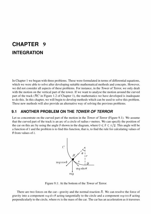
CHAPTER 9INTEGRATION
In Chapter 1 we began with three problems. These were formulated in terms of differential equations,which we were able to solve after developing suitable mathematical methods and concepts. However,we did not consider all aspects of these problems. For instance, in the Tower of Terror, we only dealtwith the motion on the vertical part of the tower. If we want to analyse the motion around the curvedpart of the track (
� �in Figure 1.2 of Chapter 1), the mathematics we have developed is inadequate
to do this. In this chapter, we will begin to develop methods which can be used to solve this problem.These new methods will also provide an alternative way of solving the previous problems.
9.1 ANOTHER PROBLEM ON THE TOWER OF TERRORLet us concentrate on the curved part of the motion in the Tower of Terror (Figure 9.1). We assumethat the curved part of the track is an arc of a circle of radius � metres. We can specify the position ofthe car on this arc by using the angle
�shown in the diagram, where � � � � � � . This angle will be
a function of � and the problem is to find this function, that is, to find the rule for calculating values of�
from values of � .
�
�
�
� � � � �
�
��
� � � � �
�
�
Figure 9.1: At the bottom of the Tower of Terror.
There are two forces on the car—gravity and the normal reaction � . We can resolve the force ofgravity into a component � � � � �
acting tangentially to the circle and a component � � � � �acting
perpendicularly to the circle, where is the mass of the car. The car has an acceleration as it traverses

168 INTEGRATION
the circle. This comes about because it is being forced to move in a circle rather than a straight lineand because its rate of traversing the circle may be changing. It can be shown that this accelerationcan be resolved into a radial component � � � � and a tangential component � � � � . Since the radius of thecircular arc does not change, the frame must apply a reaction force � � � � � � � as well as a reactionto the radial component of its weight, that is � � � � �
. The total reaction force supplied by the frameis thus � � � � � � � � � � � , so that the net radial force on the car is � � � � � . This net force keeps the caron the circle and prevents it flying off on a tangent, but does not affect its speed and plays no role inour problem. Consequently, we need only consider the tangential force � � � � � �
.Let � denote the distance along the curve from
�, the lowest portion of the curve. Using Newton’s
second law of motion we have
�� � �
� � � � � � � � � � � �If � is the radius of the circular arc and
�is measured in radians, then � � � �
and so
� � � � �
� � � � � � � � � � �
or� � � � � � � � � � � �
where � � � � # � . This is the differential equation we have to solve to find�
as a function of � . If wewere to try to solve this equation by assuming a power series for
�of the form
� � & ' � & ) � � & � � � � & + � + � , , ,for
�, we would run into difficulty with the term
� � � � � � � � . & ' � & ) � � & � � � � & + � & + � , , , 3 �The basic problem is that the differential equation is not linear and so our methods for linear equationsare not applicable. Since infinite series cannot be easily used to solve this problem, we shall developan alternative approach. Rather than leaping into the unknown by considering this problem now, it iseasier to go back to the original three problems presented in Chapter 1 and look for alternative waysof solving them. We can then return to the present problem and use our new methods to solve it. Thiswill take some time and we will not be able to complete the solution to the problem of finding themotion along the circular arc until Chapter 13.
9.2 MORE ON AIR PRESSUREThe initial value problem � 5
� 6 � 5 5 ; � = � ?arose in our discussion of the air pressure problem in Chapter 6. We solved it by a power seriesmethod to get the solution 5 � B D . We are now going to get this same result by a different method,although it will take us most of this chapter and the next to do this.
The initial condition we used was 5 ; � = � ? , so for values of 6 close to zero, 5 is not zero and wecan write the differential equation as ?
5� 5
� 6 � ? � (9.1)

MORE ON AIR PRESSURE 169
The key to the new method is to use the chain rule on the left-hand side of this equation. Suppose thatwe are able to find a function
�whose derivative is given by
� � � � � � � � . Then equation (9.1) canbe written
� � � � � � �� � � �
or�
� �� � � � � � � � � � (9.2)
We now have a new problem: find a function whose derivative is 1. Such functions are easy to find.We have
�� � � � � �
�� � � � � ! � �
�� � � � � % & � � �
and, in general,
�� � � � � � � �
for any constant � . As we shall later show, any function with derivative 1 must have the form � � � ,so let’s assume this for the moment. Then we can write equation (9.2) as
� � � � � � � � � � � (9.3)
that is,
� �� � � � � � � � � �
At this stage we know the following:
- �is an unknown function whose derivative satisfies
� � � � � � � � .
- The composition�
� � satisfies � �� � � � � � � � � .
It is not obvious that we have achieved anything. The solution � � � � that we want is tied up with theunknown function
�in the composition
�� � and it is difficult to see how to disentangle it. However,
we have identified two problems that need to be explored in greater detail.
- If we are given a function / , how do we find a function�
such that� � / ? The answer to
this question will lead us into primitive functions (or antiderivatives) and integrals, which wediscuss in the next section.
- If we know the function�
and the composition�
� � , how do we find � ? To answer thisquestion we will need to understand inverse functions. These will be discussed in Chapter 10.

170 INTEGRATION
9.3 INTEGRALS AND PRIMITIVE FUNCTIONSLet � be a given function. A function
�such that
� � � � is called a primitive, an antiderivative or anindefinite integral of � . Finding
�is the reverse of the problem of differentiation. For example, � is a
primitive of 1, � � � is a primitive of � � � � and so on. There are no comprehensive rules for findingprimitives and the process is intrinsically harder than differentiation.
The first point to notice about primitives is that they are not unique. A given function has manyprimitive functions. Thus � � , � � � � and � � � � � � � are all primitives of � � . Since the derivative ofa constant is zero, it is easy to see that we can add a constant to any primitive function to get a newprimitive function. In other words, if
�is a primitive function of � , then so is
� � � for any constant� . In fact, we have the following result.
THEOREM 9.1If
�and
�are primitives of the same function, then
� � � � � for some constant � .
This theorem is a consequence of the result (which we stated on page 100) that a function with zeroderivative on an interval is constant on the interval. Suppose
�and
�are primitives of � . Then� � � � ,
� � � � and so
�� �
� � � # � � # % � � � � # � � � # � � � # � � # � * ,Thus
� � # � � # � � , where � is a constant, and hence� � # � � � # � � .
A consequence of this theorem is that once we have found one primitive of a function, we havefound all of them. The others differ by constants. There is a special notation used for primitives. If
�is a primitive of � , we write �
� � # � � � � � # � � ,This is read as the (indefinite) integral of � � # with respect to � is
� � # plus � . Note that Mathematicadoes not put in the constant � . The notation has arisen for historical reasons and we shall have moreto say about it later.
Knowing results for derivatives enables us to find primitives:
1�
� 2 � � � � 2 4 56 � � � � 9 6 ;� �
1�
� � > � � � � �> � � � > � � �
1�
� � � > � � � � �> � � > � � �
1�
E F G � � � �> E F G � �
EXERCISES 9.3
Find primitives for the functions in Exercises 1–6.
1. � � # � � H � � � � � 2. � � # � E J G � � � � � �

AREAS UNDER CURVES 171
3.� � � � � � � � � � � � � 4. � � � � � �
� �5. � � � � � � � � 6. " � � � � � � � & �
7. A function(
satisfies( ) � + � � � + � � and
( � - � � � . Determine(
.
9.4 AREAS UNDER CURVESIn Section 9.1 we assumed it was possible to find a function
(whose derivative satisfies
( ) � � � � � 4 � .Can we in fact determine a convenient expression for
(? Certainly the primitive of
(is not a power
function since �� 5 6 � � � 5 8 9
: � � � � ; : >� � � ;where � is an arbitrary constant. It is possible that there is some complicated rational function whichwhen differentiated by chain rules, product rules and the like may, after much cancelling, end up as
� 4 � . This is unlikely. Usually the process of differentiation results in a more complicated function.In fact it can be shown (with some difficulty) that there is no function defined by an algebraic formulawhose derivative is � 4 � . So is there any such function
(at all? Around the period 1650–1670, Sir
Isaac Newton and Gottfried Leibniz developed the ideas which led to one of the great discoveries incalculus. If we are given any continuous function " , there is a way of defining a function
(such that( ) � " . This is done by a process known as definite integration and provides a third way in which to
define functions. Recall that we have so far defined functions in one of two ways:
B The simplest types of function were those defined by algebraic formulas such as
" � � � � � � � � � �� � � & D
B Functions defined by power series arose when we solved differential equations, but in generalany power series defines a function whose domain is the interval of convergence of the powerseries.
In this chapter we will show you how to use integration to produce functions having a given derivative.
� � �+ F +
� � " � � �G
H
Figure 9.2: The area under a curve
Calculus is full of surprises. One of the most fundamental of these arises as follows. Let + F be afixed point in the domain of a positive continuous function " (Figure 9.2). Consider the area
J � + � of

172 INTEGRATION
the region bounded by the graph of � , the � axis, and the two vertical lines � � � � and � � � , where� is any point in the domain of � which satisfies � � � � . We loosely refer to
� � � � as the area underthe curve � � � � � � between � � and � . Notice that in this way we can define a function (denoted by�
) if we let the ouput number be� � � � for the input number � . The surprising fact is that
� � � � .Why should this be so? A function and its primitive are connected by differentiation, which can bephysically interpreted as the slope of a curve at a given point, and this does not appear to have anythingto do with the area under the curve. It is certainly not a result we might have expected. There is aneven greater surprise in store. The connection between area and primitives is not just mathematicalentertainment. It also turns out to be useful.
Before proceeding with the full details we shall consider a few simple cases to illustrate the con-nection between primitives and area.
EXAMPLE 9.1Let � � � � � � . The region bounded by the � axis, the line � � � and the vertical line through apoint � � � on the positive � axis is a triangle with base � and height � (Figure 9.3), so that its area is� � � � � $% � % . Here we have
� � � � , so that�
is a primitive of � .
(
)�
� � � �
� � � � � �
(
)�� �
� � � �
� � � � � �
Figure 9.3: Regions under � � � � � �
EXAMPLE 9.2Let us take the same function � � � � � � as in the previous example, but this time we consider the area� � � � of the region bounded by � � � , the � axis and the vertical lines through � � � � and � � � ,
� 0 � � (Figure 9.3). It is easy to see that� � � � � $% � % 1 $% � %� 2
and that� � � � . Hence
�is again a primitive of � , but differs from the primitive in the previous
example by a constant.
EXAMPLE 9.3Let � $ � � � � 1 � . The region bounded by the � axis, the line � � 1 � and the vertical line through apoint � � � on the positive � axis is a triangle with base � and height � (Figure 9.4), so that its area is� � � � � $% � % . In this case, it is 1 �
which is a primitive of � $ , that is � 1 � � � � � $ .

AREAS UNDER CURVES 173
� �
��� � � �
� � � � � � �
Figure 9.4: A triangular region under � � � � � � �
EXAMPLE 9.4Let � � � � � � . We wish to find the area
� � � of the region bounded by the � axis, the parabola� � � � and the vertical line through a point � � � on the positive � axis (Figure 9.5). We can solvethis problem by making use of a result which has been known for over 2000 years and which was firstproved by Archimedes in about 250 BC1. Archimedes found that the area of the parabolic segment
� � in Figure 9.5 is � � � . Using this result, we see that
� � � � � � �� �� �� �� �� � � $
since � � � . We see that� ' � � , so
�is a primitive of � . )
�
� �
�
� � � �
� � � � � �
�
�
Figure 9.5: The area under a parabola
1This discovery is documented in a remarkable piece of work entitled Quadrature of the parabola. In it, Archimedesperforms what is essentially a numerical integration to reach his goal of finding the area of a parabolic segment. The significanceof his ideas were not realised until the seventeenth century when the development of the calculus occurred. Interested readersmay like to read this work, which can be found in the Encyclopaedia Britannica series, Great Books of the Western World(volume 11).

174 INTEGRATION
The key observation to be made in all of these examples is that the area of the region between thegraph of the given function and the � axis is, to within a sign, also a primitive for the function. Thisis not a coincidence; rather it is one of the most fundamental facts about the calculus and one whichwill need to be carefully investigated.
9.5 AREA FUNCTIONSLet � be a given function and let � � be a fixed, but arbitrary, point on the � axis in the domain of � .We call � � a reference point. We want to define another function
�by making use of the area of the
region bounded by the graph of � , the � axis and the vertical lines through � � and any other point � inthe domain of � , with � � � . We shall have to be careful about signs when doing this. We begin withthe most straightforward case by assuming � � � � for all � in the domain of � . Then (Figure 9.6)we define
� � � by � � � � � � � �where
� � � is the area of the region under the curve between � � and � .
� � � �
� � �
� � � � ��
�
Figure 9.6: Defining a function�
by� � � � � � �
The area� � � (and hence the function value
� � � ) is a number which can be calculated for eachchoice of � . The calculation is not always easy and we shall have to investigate methods for doing it,but for the moment let’s accept that it can be done.
� � � �� � �
� � � � �� �
�
Figure 9.7: Defining a function�
by� � � � � � �
Now let us take the case when � � � " � for all � in the domain of � (Figure 9.7). As before,choose a reference point � � and let � be any point in the domain of � satisfying � � � . Let
� � � be the

AREA FUNCTIONS 175
area of the region bounded by the � axis, the graph of � and the vertical lines through � � and � . Thenwe define
� � � by � � � � � � � � �Finally, we take the case where � � � changes sign one or more times for � � � � � � . In this case,
some parts of the region bounded by the lines � � � � , � � � , the graph of � and the � axis will lieabove the � axis, while other parts will lie below the � axis. We attach a positive sign to the area ofeach part of the region which lies above the � axis and a negative sign to the area of each part of theregion which lies below the � axis. The function
�is defined by letting its output number
� � � at thepoint � be the sum of these signed areas (Figure 9.8).
� �
� �
� ��
� � � � �
�
�
Figure 9.8: Defining a function�
by� � � � � � �
! " �#
In summary we can use the area of the region bounded by the graph of a function � , the � axis andtwo vertical lines to define a function
�. In Examples 9.1–9.4 this function
�satisfies the condition� $ � � (Exercises 9.5). There are two matters which we need to address:
& How do we calculate the area of the region under a curve in the general case? We need to beable to do this in order to calculate function values of
�.
& Does the function�
always satisfy� $ � � ?
The answers to these questions emerged with the discovery of the calculus by Newton and Leibnizin the middle of the 17th century. The answer to the first question is conceptually straightforward,although the calculations may sometimes become unwieldy. We shall address this question in thenext two sections. The answer to the second question is given by the fundamental theorem of thecalculus, which we shall discuss in Section 9.8.
EXERCISES 9.5
1. Construct the function�
described in the text of this section for each of the examples 9.1–9.4.Verify that
� $ � � in each case.
2. Use Archimedes’ result for the area of a parabolic segment to show that the area of the regionbounded by the graph of � � � � ) � # , the � axis and the vertical lines � � + and � � � is givenby
� � � � � . � 0 . Is�
a primitive of � ?

176 INTEGRATION
9.6 INTEGRATIONIn the previous sections, we have shown how it is possible to construct a function
�by using the area
(with an appropriate sign) of the region bounded by the graph of a continuous function � , the � axisand the lines � � � and � � � , where � and � are in the domain of � . The first problem to be dealtwith is to determine a method of calculating the area of a figure with one or more curved boundaries.The basic idea is to approximate the area by simple shapes whose area can be calculated and thentake a limit. This idea is a very ancient one. It was used by Archimedes to calculate the area of theparabolic segment we considered earlier.
9.6.1 Positive functions
Let � be a function defined on the interval � � � and suppose that � � � � � � for all � � � � � . We wishto determine the area of the region bounded by � � � � � � , the � axis and the lines � � � and � � �(Figure 9.9).
The simplest way to approximate the area of the region is by rectangles. Divide the interval � � �into " subintervals
� � & � � & � ) � + + + � - / & � - � where � � � and � - � � . The intervals need not be of the same length. In each subinterval � � / & � � �( � � 6 8 + + + " ), select an arbitrary point � �� and form the sum
: � " � � � � � �& � � � & > � � @ � � � �) � � � ) > � & � @ � � � �C � � � C > � ) � @ D D D @ � � � �- � � � - / & > � - �� � � � �& � G � & @ � � � �) � G � ) @ � � � �C � G � C @ D D D @ � � � �- � G � -
�-�
� H &� � � �� � G � �
whereG � � � � � > � � / & , � � 6 8 + + + " . Such a sum is called a Riemann sum. It is the sum of
M
N� & � ) � C � O� �� � & � �) � �C � �O � �P
� � � � � �
Figure 9.9: Approximating the integral by a Riemann sum
the areas of the individual rectangles shown in Figure 9.9. Such sums approximate the area under thecurve and it seems intuitively clear that the approximation converges to the exact value of the area aswe take more intervals in such a way that their number increases without limit and such that they allget arbitrarily small. This is true if � is continuous. However, it is quite difficult to prove this, since

INTEGRATION 177
we have to consider all the possible ways in which the intervals become small and increase in number.We shall omit the detail on how to do it in a mathematically correct way and simply write� �
� � � � � � � � �� � � � �� � �� �� � � �
� � � � � � � � � � � � � � � � (9.4)
The expression on the left-hand side is called the definite integral 2 of � on the interval ! # % ' . Thenumbers ! and % are called the limits of integration. We call ! the lower limit and % the upper limit.
The process of using Riemann sums to compute integrals can be simplified considerably if wetake intervals of equal width. Begin by dividing the interval ! # % ' into ( subintervals
� � # � � ' # � � # � . ' # � � � # � � � � # � � ' #of width 1 � % � !
( #where � � ! and � � % .
There are now two obvious ways to approximate the area by rectangles. Firstly, we can userectangles of height � � � � � � � and base
1 � , ( 9 # : # � � � # ( ). This gives the following approximationto the area under the curve
; � � ( � � � � � � 1 � A � � � � � 1 � A C C C A � � � � � � � 1 � % � !
( D � � � � � A � � � � � A C C C A � � � � � � � F � (9.5)
The particular Riemann sum ; � � ( � is called a left-hand sum, because we have used the value of thefunction at the left-end of each interval. This approximation is illustrated in Figure 9.10.
G
H! %� � � . � I � J � K
L � � � �
1 �
Figure 9.10: The integral approximated by a left-hand sum
Alternatively, we can calculate a right-hand sum by using the rectangles of height � � � � � and base
2The integral sign � was first used by Leibniz on October 29, 1675. It was an elongated “S”, for the word “sum”.
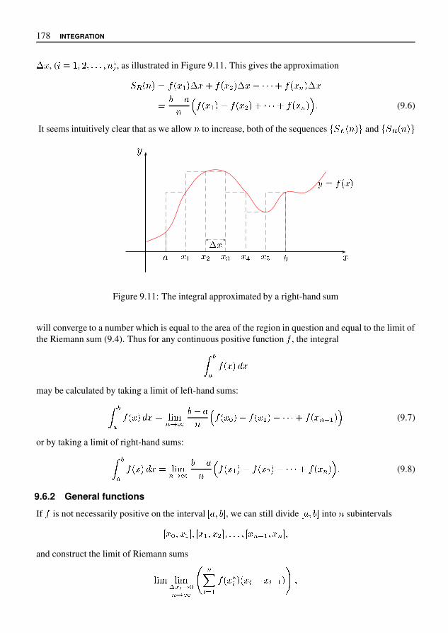
178 INTEGRATION
� � , ( � � � � � � � � , as illustrated in Figure 9.11. This gives the approximation
� � � � � � � � � � � � � � � � � � � � � � ! ! ! � � � � $ � � �� & ( *
� + � � � � � � � � � � � � ! ! ! � � � � $ � , (9.6)
It seems intuitively clear that as we allow � to increase, both of the sequences - � � � � � / and - � � � � � /1
2* &� � � � � 3 � 4 � 5
6 � � � � �
� �
Figure 9.11: The integral approximated by a right-hand sum
will converge to a number which is equal to the area of the region in question and equal to the limit ofthe Riemann sum (9.4). Thus for any continuous positive function � , the integral� �
9 � � � � : �may be calculated by taking a limit of left-hand sums:� �
9 � � � � : � � = > ?$ @ B & ( *� + � � � C � � � � � � � � ! ! ! � � � � $ E � � , (9.7)
or by taking a limit of right-hand sums:� �9 � � � � : � � = > ?$ @ B & ( *
� + � � � � � � � � � � � � ! ! ! � � � � $ � , (9.8)
9.6.2 General functions
If � is not necessarily positive on the interval H * � & J , we can still divide H * � & J into � subintervals
H � C � � � J � H � � � � � J � � H � $ E � � � $ J �and construct the limit of Riemann sums
= > ? = > ?� N @ C$ @ B� $� P �
� � � � � � � ( � E � � � �

INTEGRATION 179
where � �� is an arbitrary point in the � � th subinterval. As long as the function � is continuous on � � � � ,it can be shown that such a sum will converge and once again we denote the value of this sum by� �
� � � � � � �
As before, we call this the definite integral of � on the interval � � � � . However, the interpretation ofthe integral is now different. In this case, some parts of the region bounded by the lines � � � , � � ,the � axis and the graph of � may lie above the � axis, while other parts may lie below it. We attacha positive sign to the area of each part of the region which lies above the � axis and a negative signto the area of each part of the region which lies below the � axis. The integral is then the sum ofthese areas, taking the sign into account. This statement follows directly from the way in which theRiemann sum was constructed. If, for example, � � � � � � for all � � � � � , then the limit of the sumin equation (9.4) will be negative.
There are some minor points to clear up. In the above discussion, we have assumed that # � inthe integral � � � � � � � � . If this is not the case, we simply define � � � � � � � � for � � by� �
� � � � � � � '�
� � � � � � � �
Also, for equal upper and lower limits, we define� � � � � � � � � �
9.6.3 Some properties of integrals
There are some other properties of integrals which we now state. First, there are the results for sumsand multiples: � �
) � � � � + - � � � 0 � � �
� � � � � � � � +
� � - � � � � �
and � � � � � � � � � � �
� � � � � � � � �
where � is any constant.These results can be proved in each case by expressing both sides either as the limit of a left-hand
sum or as the limit of a right-hand sum and showing that these limits are equal.There are no results for integrals of products and quotients which apply in all cases.If we take a point � with � � � � , then� �
� � � � � � �� �
� � � � � � +� �
� � � � � � � �
If � is positive, then this result amounts to the addition of areas, but the same result holds whatever theorder of � , and � and whatever the sign of � . The use of left-hand or right-hand sums is inadequateto prove this result. A correct proof would need to use more general Riemann sums.

180 INTEGRATION
We can now return to the area functions we were discussing in Section 9.5. For any continuousfunction � with domain � � � � we can define a function
by
� � �� �
� � � � � � � � � � � � !The discussion in Section 9.5 shows that the number
� � can be interpreted physically in terms ofthe area of a region bounded by the the graph of � and the vertical lines � � � and � � . Functionsdefined in this way will play a major role in the remainder of this book and it is important that youunderstand this process.
In general, integrals cannot be calculated exactly except in special cases. This is because noformula can be found for the Riemann sum and so there is no way of calculating the limit. We cancompute approximate values to any required degree of accuracy by choosing sufficiently large valuesof % . These calculations are usually very tedious to do by hand and a computer is needed.
EXAMPLE 9.5Evaluate � &
'(� � �
approximately.Here � � ( , � � - . We choose % � ( 1 , so that the width of the subintervals is 2 � & 4 '' 5 � 1 ! ( .
Then � &'
(� � � � 1 ! ( : (( ! 1 ; (( ! ( ; (( ! - ; < < < ; (( ! ? A !� 1 ! B ( ? !If we choose % � - 1 ( 2 � 1 ! 1 H ) we obtain 0.706 for the approximation while if we choose % � ( 1 1( 2 � 1 ! 1 ( ) we obtain 0.696. The sequence of values appears to be converging, but very slowly. Thereare various ways to improve the approximation and we shall deal with these in the next section. J
In some special cases, it is possible to use formulas such as
( ; - ; N ; < < < ; % � P�� Q '
R � '& % � % ; ( � (9.9)
( & ; - & ; N & ; < < < ; % & � P�� Q '
R & � 'V % � % ; ( � � - % ; ( � (9.10)
( Z ; - Z ; N Z ; < < < ; % Z � P�� Q '
R Z � '\ % & � % ; ( � & (9.11)
to evaluate integrals explicitly by finding an expression for a left-hand or right-hand sum and thentaking a limit. The above formulas can be proved by the use of mathematical induction.
EXAMPLE 9.6Evaluate � '5 � � � � � � �where � � � � � � & .

INTEGRATION 181
Solution. We divide the interval � � � � � into subintervals of width � � . Then using equation (9.8)with � � , � � � , � � � � � , � � � � � , � � � � � � � , we find� �! � � " � � & ' (� ) + � � , - , � / 0 - , � / 0 3 3 3 0 - 4 5 / �� & ' (� ) + � � , � � 0 � � � 0 7 � � 0 3 3 3 0 � � / �� & ' (� ) + � � 8 9 � � 0 � � 0 7 � 0 3 3 3 0 � < �� & ' (� ) + � � 8 = ? 0 � B ? � 0 � BD �� �7 �Thus � �! � � " � � �7 �Note that this gives Archimedes’s formula quoted earlier.
EXERCISES 9.6
Evaluate the sums in Exercises 1–9.
1.� !�� E � ? 7 G I � B 2.
� ��� E � ? � 0 7 B 3.� ��� E � ? G I � B �
4.L�
� E � ? M 0 � B ? M I � B 5.O� E � ? � 8 I � � � B 6.
� E � !�� E Q ? G � 0 7 G B7.
� !�� E S G 8 8.
��� E � ? G I B � 9.��� E � ? G � 0 � B
10. Determine the limits of the following sequences.
(a) T � 0 � 0 7 0 3 3 3 0 � X(b) T � � 0 � � 0 7 � 0 3 3 3 0 � 8 X(c) T � 8 0 � 8 0 7 8 0 3 3 3 0 8 Q X
In each of the following exercises, find the area of the region under the graph of - from � � to� � � by expressing the integral as the limit of a sum.
11. - ? � B � 7 � 0 � � � � � � � `

182 INTEGRATION
12. � � � � � � � � � � �13. � � � � � � � � � � �14. � � � � � � � � � � � � � � � �15. � � � � � � & � � � � � (16. � � � � � � & � � � � � � -
9.7 EVALUATION OF INTEGRALSIn this section we shall assume for simplicity that all functions are positive. The formulas we get willhold even when this restriction is lifted, but we shall not prove it here.
9.7.1 The trapezoidal rule
It would appear from a consideration of Figure 9.12 that a better approximation to the area undera curve would be obtained if we used trapeziums instead of rectangles. Trapeziums are four-sidedfigures with a pair of parallel sides. To get an approximation to �
.� � � � � 0 � we divide the interval1 � � � 5 into 6 subintervals of width 7 � � & � � < 6 and approximate the region under the curve between� � and � � by trapeziums, as shown in Figure 9.12. The area of a trapezium is easily derived by
dividing it into two triangles and a rectangle. In the notation of the right-hand diagram in Figure 9.12,the area is found to be > 7 � � � � � . Using this result, we see that the area of a typical trapezium inFigure 9.12 is > 7 B � � � � C > � � � � � � � G , where � I � I 6 .
J � � � �L
M� O � > � � P � Q7
��Area > 7 � � � � �
Figure 9.12: Approximating a region by trapeziums
Let � T denote the sum of the areas of all such trapeziums. Then � T is an approximation to�
�. � � � � 0 � . We find that
� T 7 �B � � � O � � � � � > � G � 7 �
B � � � > � � � � � � G � U U U � 7 �B � � � T C > � � � � � T � G
7 � Y � � � O � � � � � � > � � � � � � � � U U U � � � � � T C > � � � � � T � Z (9.12)
Equation (9.12) is known as the trapezoidal rule.

EVALUATION OF INTEGRALS 183
EXAMPLE 9.7Approximate � �
��� � �
using the trapezoidal rule for the cases � � � , � � � and � � � � .Solution. For � � � , we have
� � � � � �� � �� � � � �� � � � �� � � � � � � � �� � � � �� � � � � � � � � ! �For � � � , we find � � � � � � � � "while for � � � � � � � � � � � � � � �The convergence is far more rapid than for the rectangle approximation.
9.7.2 Simpson’s rule
An even better approximation is to take points three at a time and fit a parabola through them. Toapproximate � �
% & ( � + � �we divide the interval , - " 0 1 into an even number of subintervals. Let
� � - " � � " � � " � � � " � 6 8 � " � 6 0be the end points of these subintervals, where � is an even integer.
� � �
� � 8 � � � � � : � ;
<
= & ( � +
Figure 9.13: A parabolic approximation to part of the graph of = & ( � + .
For a typical triplet > � � 8 � " � � " � � : � ? ( � � " � " � � � " � C � ), we pass a parabola through the points( � � 8 � " & ( � � 8 � + + , ( � � " & ( � � + + and ( � � : � " & ( � � : � + + and then find the area of the region bounded by thisparabola, the � axis and the lines � � � 8 � and � � � : � (Figure 9.13). We can use the result
184 INTEGRATION
of Archimedes mentioned earlier to do this. Denote the sum of these areas by � � . Then � � is anapproximation to the integral � �� � � � � and we find, after some effort, that
� � � � � � � � � � � � � � � � � � � � � � � � � ! � � # # ## # # � � � � � & � � � � � � & � � � � � � � ( # (9.13)
Equation (9.13) is known as Simpson’s rule.3 It is sufficiently accurate for many practical purposes,but there are times when more sophisticated methods are needed. We shall not discuss these here. Bychoosing successively smaller values of � we look for a sequence of constant output numbers fromthe application of Simpson’s rule.
EXAMPLE 9.8Take ) � , . , ) � � . and ) � , . . in Simpson’s rule to approximate the integral�
�, � #
We have
� � � � . # ,� 3 ,, � �, # , � �, # � � �, # � � 4 4 4 � �, # 5 � ,� 6 #� . # 8 5 � , 9 . #For ) � � . we find � � #� . # 8 5 � , � :and for ) � , . . � � � � #� . # 8 5 � , � : #We conclude that the value of the integral is 0.6931 to 4 decimal places.
In using approximations such as the trapezoidal rule or Simpson’s rule, questions regarding theaccuracy of these rules naturally arise. Let � be a function with domain < = > @ A . Let � � and � � respec-tively denote the trapezoidal estimate and Simpson’s estimate for � �� � � � � # We can write� �
� � � � � � � � � E � � � �and, for even values of ) , � �
� � � � � � � � � E � � � � #Thus H E � � � � H is the numerical difference between the actual value of the integral and the trapezoidalestimate with ) subintervals, while H E � � � � H is the numerical difference between the actual value of theintegral and Simpson’s estimate with ) subintervals.
We state the following two results without proof.J Suppose that � K K is continuous on < = > @ A and that there is a constant � such that H � K K � � H L �for all in < = > @ A . Then
H E � � � � H L � � @ N = � !, � ) #3Thomas Simpson (1710–1761) was a weaver who taught himself mathematics. The rule which we know by his name was
known to Gregory and Cavalieri in the seventeenth century, but Simpson popularised it in his book A new treatise on fluxions.
EVALUATION OF INTEGRALS 185
� Suppose that � � � � is continuous on � � � � and that there is a constant�
such that � � � � � � � � �for all � in � � � � . Then, if � is even
� � � � � � � � � � #$ & ( � � *EXAMPLE 9.9Estimate the error in applying the trapezoidal rule with 10 subintervals to the integral� +
,$� - � *
Solution. We put � � � � 0 $ 3 � , so that
� 5 5 � � � 0 77778� 9 7777� 8
on the interval � $ � 8 � . Consequently, using the above error estimate with � 0 8 , � 0 $ and 0 8gives
� � � � � � 8 � 8 $ � 9$ 8 C $ ( +*0 ( * ( ( $ E *Hence, using the result from Example 9.7, we have� +
,$� - � 0 ( * H I J & L ( * ( ( $ E *
EXERCISES 9.7
In the problems below, calculate both the trapezoidal approximation � � and Simpson’s approximation� � to the given integral. Use the indicated number of subintervals and round the answers to 4 decimalplaces.
1.
� 9, � + - � � � 0 Q 2.
� ,R S U V � - � � � 0 H
3.
� ,R
$$ [ � + - � � � 0 Q 4.
� ,R ] $ [ � - � � � 0 Q
The next two exercises give tabulated values for a function � . Calculate an approximation to� �_ � � � � - �
using (a) the trapezoidal rule and (b) Simpson’s rule.
5. � 0 $ , 0 8 * ` (

186 INTEGRATION
� � � � � 1.25 1.50 1.75 2.00 2.25 � � � �
� � � 1.41 1.50 1.58 1.66 1.73 1.80 1.87
6. � � � , � � � �
� 0 1 2 3 4 5 6 7 8 9 10
� � � 0 � � � � � � � � � ! � � � � � � � � � % 0 81 200
7. Two students are standing on a bridge over a creek. They decide to measure the volume of waterflowing under the bridge in the following way. First, they measure the velocity of the water bythrowing twigs into the water and timing how long it takes for them to pass under the bridge.They find the average velocity to be 0.5 m/sec. Next, by using a long rod, they measure thedepth of water at various points along the width of the creek and derive the profile shown in thediagram, where all depths are given in metres. The creek is 8 metres wide. Use Simpson’s ruleto calculate the volume of water per second flowing under the bridge.
0.51.2
1.5 2.0 2.0 2.5
1.5
8. A function is given by the rule
� � � �
�'
() � + - / 0 1 2 1 �
Use Simpson’s rule to evaluate � 5 � .
9. Determine how large 6 must be in order to guarantee that the trapezoidal estimate � 8 for theintegral �
9
(
��
2 �
differs from its true value by no more that 0.0005.
10. Determine how large 6 must be in order to guarantee that Simpson’s estimate : 8 for the integral�9
(
��
2 �
differs from its true value by no more that � � ; < .

THE FUNDAMENTAL THEOREM OF THE CALCULUS 187
9.8 THE FUNDAMENTAL THEOREM OF THE CALCULUSWe are now in a position to be able to solve the following problem raised in Section 9.2:
Given a function � , find a function�
such that� � � � .
The following theorem provides the answer.
THEOREM 9.2 The fundamental theorem of the calculusIf � is continuous on the interval � � � and if
�is defined by
� � � � �� �
� � � � � � �
for � � � � � then� � � � � � � � � � !
The function�
is well defined because we can calculate its function values by procedures such asSimpson’s rule. The theorem is proved using differentiation by first principles. We will only give anoutline of the proof without going into detail. Take a sequence " $ & ' converging to zero. By definition
� � � � � � ( ) *& + -.
$ &0 � � � 2 $ & � 6 � � � � 7 !
Using differentiation by first principles, we consider
.$ &
0 � � � 2 $ & � 6 � � � � 7 � .$ &
� � � : � �� � � � � � � 6
� �� � � � � � � �
� .$ &
� � � : � ��
� � � � � � �Now if $ & is very small, then this integral is approximately $ & < � � � � . Thus
.$ &
0 � � � 2 $ & � 6 � � � � 7 � .$ & $ & � � � � � � � � � !
Taking the limit carefully as > @ B (and this is where we gloss over the detail) we find that theapproximation becomes an equality, that is
( ) *& + -.
$ &0 � � � 2 $ & � 6 � � � � 7 � � � � � !
Hence � � � � � � � � � � !Another way of writing this result is
�� �
� �� � � � � � � � � � � � !
EXAMPLE 9.10Find a function
�such that
� � � � � � .� !

188 INTEGRATION
The function we are seeking follows directly from the fundamental theorem of the calculus. It is
� � � � �� � � � �
where � is any positive constant and � is any number in � � � � � .
EXERCISES 9.8
Find the derivative of each of the functions in Exercises 1–8.
1. � � � � ��
� � � � � � � � 2. � � � �� " � � � % ' ( * � � �
3. � � � � ��
, - � . �� � / � 4. � � � � �� �
� � � � 1 , � �5. � � � � �
� �" � * � � � � � 6. 7 � 9 � �� � � �
� % ' ( � � �7.
; � � � �� � < � � � . 9 � � � 9 8. � � � � �
� �� � � � � �
9.9 THE LOGARITHM FUNCTIONThe above example gives us a lead-in to the logarithm function. Let us define a function ? @ A � withdomain � � � � � by
? @ A � ��
�� � � C
This function is often denoted by ? ( � . The function value ? @ A � is equal to the area of the region underthe curve D � � G � between the vertical lines � � � and � � � (Figure 9.14) and is calculated by, forexample, Simpson’s rule. It follows from the definition and the fundamental theorem of the calculusthat � � ? @ A � � � �� C (9.14)
EXAMPLE 9.11In Example 9.8, we found � �
��� � C� � C K L M �
to 4 decimal places. We conclude that ? @ A * C� � C K L M � .Similar calculations give
? @ A �� �� ��
�� � �
� .� �
��� � �
C� . � C K L M � C

THE LOGARITHM FUNCTION 189
� � ��
� ��
�
�
� � �
Figure 9.14: The logarithm function
and
� � � � �� � � �
��� � �
�� � � � � � � ��
Let’s now return to the matter of solving the initial value problem
� �� � � � " � % ' ( � � �
In Section 9.2 we showed that by choosing a function)
such that) * % � ( � � . � , we could write the
above differential equation as�
� �0 ) % � % � ( 2 � � " (9.15)
from which we found ) % � % � ( ( � � 8 � �We now know that
) % � ( � � � , so we can write
� % � % � ( ( � � 8 � �To get the constant � we use the initial value � % ' ( � � to get � � � ' 8 � . It follows fromthe definition of � � that � � � ' , so that � � ' . The solution to the initial value problem is � � % � ( � � .
The only problem that remains is to write the unknown function � explicitly in terms of � , thatis, to extract the � % � ( from inside the logarithm. In order to do this, we will need to derive someproperties of the logarithm function. In the next chapter we will discuss the matter of writing �explicitly in terms of � .

190 INTEGRATION
The graph of � � � � crosses the � axis at the point � � . In fact, it follows from the definition ofthe logarithm in terms of integrals that
� � � � � if � �� � � � � � if � � � � �
� � � � � �
Since the domain of � � � � is � � � � , the graph does not cut the ! axis.
We can also find the concavity of the graph of � � � � . Since
"" � � � � � � �
� � " %" � %
� � � � � � ' � %
we have
"" � � � � � � � � " %
" � %� � � � � � �
for all � � , that is, for all � in the domain of � � � � . Thus the graph is increasing and concave downfor all � � . As � gets close to zero, the slope of the graph increases and approaches infinity. Itis not yet clear what happens as � becomes arbitrarily large. Does the slope of the graph approacha number, or does it become arbitrarily large? A software package such as Mathematica has thelogarithm function built in, and we can use it to plot the graph in Figure 9.15. In principle you couldplot such a graph by using Simpson’s rule to calculate � � � � for different � values, plotting these pointsand then joining them with a smooth curve. In fact, this is what Mathematica essentially does.
+ , -�
+
'
' +
! � � � � �
1
2
Figure 9.15: Graph of ! � � � � �

THE LOGARITHM FUNCTION 191
THEOREM 9.3 Properties of log �For all positive numbers � and � and all rational numbers � , we have
� � � � � � � � � � � � � � �
� � � �� � � � � � �
� � � �� � � � � � � � � � �
� � � � � � � � � � � �
To prove this, consider the function� � � � � � � � � � � � � � . Using the chain rule we have
� % � � � && � � � � � � � � � � � � � �
� � � � �� � *
Since � � � � � � � � � � has derivative zero, we have � � � � � � � � � � � � for some constant � . To find� , put � � � . Then � � � � � � , so � � � � � � � � � � � � � � � . Finally, put � � � and rearrange the lastequation to get
� � � � � � � � � � � � � � � �
Next we have
� � � �� � � � � � � � � � �
� �
� � � � �� * 9
so that
� � � �� � � � � � � �
The next identity in Theorem 9.3 now follows easily:
� � � �� � � � � � �
�� � � � � � � � � �
�� � � � � � � � � � �
The final identity of Theorem 9.3 is proved in a number of stages. Here we will only prove theresult if � is an integer. If � is a positive integer ; we have
� � � � < � � � � � � > � > @ @ @ > �� � < terms
� � � � � � @ @ @ � � � � �� � < terms
� ; � � � � �

192 INTEGRATION
Next, if � is a negative integer � , we can write � � � � , where � is a positive integer. Then
� � � � � � � �� � � ��� � � �� �
�� � � � �� � � � �
We have shown that � � � � � � � �where � is any non-zero integer. That the result is also true if � � is left as an exercise.
We shall show on page 205 that this result holds for all rational numbers � . It is also true if � isany real number, but we will not go into detail on this matter.
Questions about the behaviour of � ! for large and small values of ! can now be answered. Since � # � � ' ( ) , we have � # � � � ' ( ) * � , so � ! gets arbitrarily large as ! increases. This isusually written + ,- . 0 � ! � 3 �Similarly, � # � � � � � ' ( ) * � , so � ! gets arbitrarily small as ! gets closer to zero. We writethis as + ,- . 6 � � ! � � 3 �The notation ! 9 ; is used to emphasize that ! can only approach zero through positive values.
9.9.1 The indefinite integral of � = !We have shown that ?? ! @ � ! B � �! �In this equation, we must have ! D in order for � ! to be defined. Thus� �! ? ! � � ! E � � ! D � (9.16)
If ! G , we put I � � ! , so that I D . Then
?? ! @ � @ � ! B B � ?? I @ � I B ? I? !� �I @ � � B� �! �
Hence � �! ? ! � � @ � ! B E � � ! G � (9.17)

THE LOGARITHM FUNCTION 193
We can combine equations (9.16) and (9.17) into the single equation��
� � � � � � � � � � � � �� � � (9.18)
The graph of � � � � � � is shown in Figure 9.16.
� � � �� �� �� �� �� $
�
�
� �
� �
� � � � � �
&
'
Figure 9.16: The graph of � � � � � �
9.9.2 Logarithmic differentiation
Logarithmic differentiation is a technique for simplifying the process of finding a derivative in certaincases. If we are given ( ) � , and want to find ( . ) � , , it may be easier to begin by finding the derivativeof � ( ) � , . The process is best illustrated by example.
EXAMPLE 9.12Find ( . ) � , if
( ) � , � ) � � � , ) � � � ,) � � � , ) � � � , �
Solution. We take logarithms to get
� ( ) � , � � � ) � � � , ) � � � ,) � � � , ) � � � , �
� � ) � � � , � � ) � � � , � � ) � � � , � � ) � � � , �
Differentiating both sides of this equation gives
( . ) � ,( ) � , � �
� � � � �� � � � �
� � � � �� � � �
Hence
( . ) � , � ( ) � , � �� � � � �
� � � � �� � � � �
� � � �� ) � � � , ) � � � ,
) � � � , ) � � � , � �� � � � �
� � � � �� � � � �
� � � � �

194 INTEGRATION
EXERCISES 9.9
Differentiate the functions given in Exercises 1–11.
1. � � � � � � � � � � � � � 2. � � � � � � � � � � � � �3. � � � � � � � � � � � � � 4. � � � � � � � � � � � � � �5. � � � � � � � � � � � � � � � 6. � � � � � � � � � ! � � � � �7. � � � � � � � � � �� # � 8. � � � � � � � % � � � �� # � �9. � � � � � � � � � � � � � � � � � ' � 10. � � � � � � � � � � � � � ' � � � # � � �
11. � � � � � � � � � � , - . �Logarithms have a number of applications. For physiological reasons, scales of luminosity and soundare often measured logarithmically. Suppose the eye is presented with a series of lamps of absolutebrightness one, two, three, four, / / / units, all at the same distance, and then with another series oflamps of brightness one, two, four, eight, / / / units, then it is the second series and not the first whichwill appear to form a uniform gradation of brightness. Similar conclusions apply to sounds. Theseconsiderations are the reason we adopt the stellar magnitude scale for measuring the brightness ofstars and other celestial objects and the decibel scale for the measurement of sound.
12. In 200BC, the Greek astromomer Hipparchus, wishing to describe the brightness of stars, classi-fied them in terms of magnitudes. The brightest stars were said to be of first magnitude. The nextgroup of prominent, but less bright stars were classified as being of the second magnitude, andso on, down to the stars which are just visible to the naked eye, which were classified as being ofthe sixth magnitude.In the nineteenth century, when accurate measurements became possible, it was found that a sixthmagnitude star was almost exactly 100 times fainter than one of the first magnitude. In fact, thefollowing table of relative brightnesses was constructed.
Magnitude 1 2 3 4 5 6Brightness 100 40 16 6.3 2.5 1
(a) By what factor does the brightness of a star change for a unit change in magnitude?
(b) Plot a graph of the logarithm of the brightness against the magnitude. What type of graphdo you get?
(c) Show that if1
is the brightness of a star, scaled to 100 for first magnitude stars, and 2 isits magnitude, then � � 1 / 4 / 4 7 # : / < � 2 /
13. The stellar magnitude scale described in the previous example can be extended at both ends. Aseventh magnitude star is 2.512 times fainter than a sixth magnitude star. It would only be visiblein a telescope. Similarly, a star of magnitude zero is 2.512 times brighter than one of the firstmagnitude and a star of magnitude # � is 2.512 times brighter again. On this scale the sun is ofmagnitude # � @ / A .

THE LOGARITHM FUNCTION 195
(a) Show that if a star of magnitude � � has brightness�
� and a star of magnitude � � hasbrightness
�� , then
� ��
���
�� � � � � � � � � � � �
(b) Let� �
denote the brightness of the sun and let� �
denote the brightness of the fainteststar visible to the naked eye. Compute � � � � � � � � � . By trial and error with your calculator,determine
� � � � �. What is the physical meaning of this ratio?
14. In land animals it is found that the leg diameter is (not surprisingly) related to the body mass.Leg thickness increases in proportion to the body mass rather than to the linear dimensions of theanimal, so that large animals, such as elephants, have relatively thicker legs than smaller animals,such as dogs. Here is a table giving the leg bone circumference (in centimeters) and body mass(in kilograms) for a selection of animals.
Mouse Cat Human Horse Hippo ElephantLeg circumference 0.6 4.5 13.6 27.4 40 80.5Body mass 0.05 3.5 50 350 1700 6000
(a) Plot the logarithm of the leg circumference on the vertical axis and the logarithm of thebody mass on the horizontal axis. You should find that relationship between the variablesis approximately linear. Use Mathematica to find the best straight line through the pointsyou have plotted.
(b) What do you notice about the plotted point for the hippopotomus? Suggest a reason foryour observation.
(c) A fossil leg bone of a Brachiosaurus was found to havea circumference of 1.33 metres. Estimate the massof the animal when it was alive. The Brachiosauruswas one of the largest land animals of all time,although some incomplete fossil skeletons suggestthat larger animals may have existed.
196 INTEGRATION
15. The range of human hearing is impressive. If the intensity of sound is measured in watts persquare metre, a normal person can just detect a noise of 10 � � � W/m � . Permanent ear damagewould occur at 100 W/m � . As mentioned above, the ear perceives sounds logarithmically andthis has given rise to the decibel scale. If � � is the intensity of a reference sound and � is ameasured sound, then the difference between � and � � in decibels is given by
� � �� � � � �� � � �(a) Take � � � � � � � W/m � as the reference point on the decibel scale. The noise caused by
a jet aircraft take-off at 60 m is 130 db. Compute the intensity of this sound in watts persquare metre.
(b) A pneumatic riveter has a noise level of 10 W/m � . Express this noise level in decibels.

CHAPTER 10INVERSE FUNCTIONS
In solving the initial value problem� � � � � � � � �
we obtained � � � � � � � . The remaining problem we have is to extract � from this equation. This isdone using inverse functions.
Let’s start with some simple cases which have a similar pattern to this one. We want to solveproblems of the following type:
� A function�
is given.
� We know� � � � � .
� How do we find � ?
EXAMPLE 10.1Suppose
� � � � � " . Then if� � � � � , we have
� � � " � �
and so� � � &
' � ) " ,
We let� � � &' � ) " . Then
� � � � � gives � � � � � .
EXAMPLE 10.2Let
� � � � ) / and suppose that� � � � � . Then
� � ) / � �
and so� � � � / ,
We let� � � � / . Then
� � � � � gives � � � � � . 4

198 INVERSE FUNCTIONS
What is the relationship between the functions�
and�
in these examples? We can answer thisquestion by applying the two functions in succession. Using
�and
�from Example 10.1 we have
� � � � � � � � � � � � � � � � � � � � � � � � �� � � � � � � � � � � � � � � � � � � � � � � � � !
These relationships are illustrated in the diagram below.
�" �� # " � � $ � "
�" � " � � "
Figure 10.1: The action of a function and its inverse
Similarly, using�
and�
from Example 10.2 gives
� � � � � � � � � � � & � � � & & �� � � � � � � � � � & � � & � & � !
In both these cases each function has the effect of reversing the action of the other. If we thinkof a function as a set of operations which starts with an input number, operates on it and produces anoutput number then, in the above examples, the other function reverses these operations and producesthe number we started from. Functions which have this property are called inverse functions;
�is the
inverse of�
and�
is the inverse of�
. We normally write� - instead of
�for the inverse of
�. A
function�
and its inverse� - are related by the pair of equations
� � � - � � � � � .� - � � � � � � � !This is illustrated in terms of function machines in Figure 10.2. We will postpone a more precisedefinition of inverse functions to the next section.
The notation� - � � � for the inverse function is universally used. Unfortunately, there is the
danger of confusing it with the reciprocal of� � � � , that is, with / 0 � � � � . You should note carefully
that the / in the notation for the inverse is not an exponent. The symbol� - � � � does not mean
/ 0 � � � � . If we do want to express / 0 � � � � in exponent form we will write 1 � � � � 3 - .
EXAMPLE 10.3Let 4 � � � � � � & . Find the inverse 4 - of 4 .
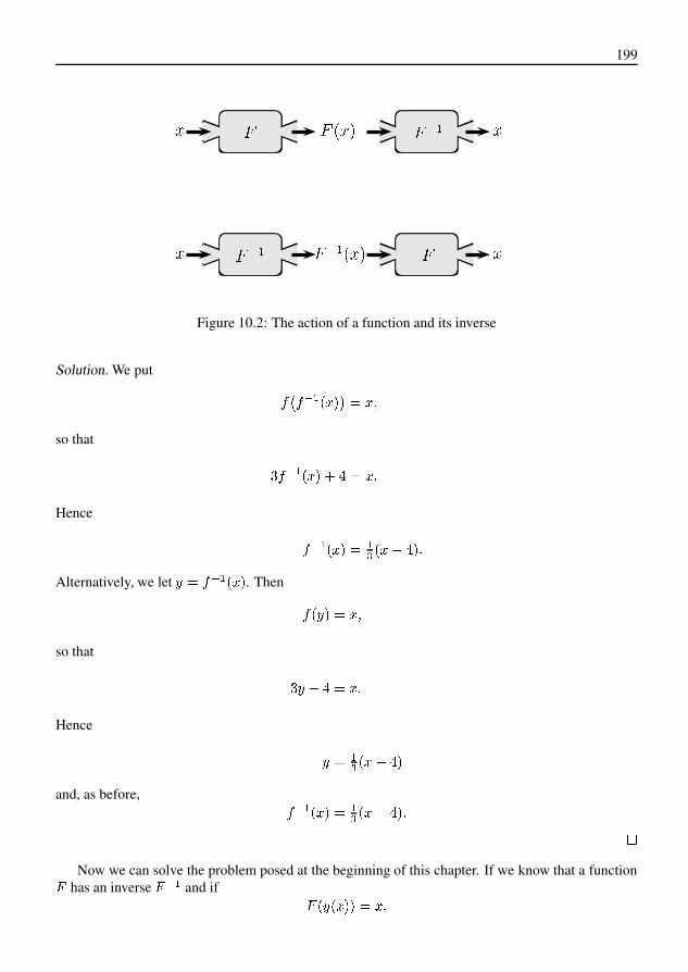
199
�� � � � � � �� �
� ��� � �
� � � � � �
Figure 10.2: The action of a function and its inverse
Solution. We put
� � � � � � � � � �
so that
� � � � � � � � � �
Hence
� � � � � �� � � �Alternatively, we let $ � � � � � . Then
� $ � � �
so that
� $ � � � � �
Hence
$ � �� � � and, as before,
� � � � � �� � � �-
Now we can solve the problem posed at the beginning of this chapter. If we know that a function.has an inverse
. � � and if . $ � � � �

200 INVERSE FUNCTIONS
then, applying� � � to both sides of this equation, gives us
� � � � � � � � � � � � � � �
Hence, since� � � undoes the action of
�,
� � � � � � � � �
The initial value problem
� � � � � � � �
thus has solution
� � � � � � � � � � �
This is all very well, but we now have two more problems to deal with. (Will this never end?)
� How can we be sure that a given function has an inverse?
� How can we calculate function values for the inverse, assuming it exists?
10.1 THE EXISTENCE OF INVERSES
Consider the function defined by � " $ " ' ) . If we pick any output number � and put � " � ,then there is only one input number " which will give this output number. For example, if � ) , then
� " ) implies that " � . On the other hand, if we take the function . � " " / , then there are twoinput numbers for each nonzero output number. For example, if � 1 , then " 2 $ . If . were to havean inverse . � � , then this inverse would satisfy . � � � . � $ $ and . � � � . � 8 $ 8 $ . This wouldrequire . � � � 1 $ and . � � � 1 8 $ , which is impossible, because functions must give a uniqueoutput number for each input number. Hence in this case there can be no such function . � � and thefunction . does not have an inverse. These arguments can be generalised to show that a function canhave an inverse only if each output number comes from a unique input number. A function with thisproperty is said to be one-to-one. We write 1–1 rather than one-to-one.
There is a graphical interpretation of 1–1 functions. Any function has the property that an inputnumber gives only one output number, so that any vertical line will intersect the graph of the functionin at most one point. A 1–1 function has the additional property that any horizontal line intersects thegraph at most once. In Figure 10.3, the graph on the right is not 1–1, while the graph on the left is1–1. You are asked to show in the Exercises that a function which is either increasing on an interval >or decreasing on an interval > will be 1–1 on > . Hence if the derivative of a function has constant signon an interval > , then the function will be 1–1 on > . This test cannot be applied if the function is notdifferentiable at one or more points and other methods are needed.

THE EXISTENCE OF INVERSES 201
� �
� �
(a) (b)
Figure 10.3: (a) A 1–1 function. (b) A function which is not 1–1.
We are almost ready to give a formal definition of an inverse function. First, we state the followingresult.
THEOREM 10.1 Let � be a 1–1 function. Then there is a unique function � whose domain is therange of � and which satisfies the equation
� � � � � � �
for all in the range of � .
The proof is straightforward. If is in the range of � , then it must come from some input numberin the domain of � . Since � is 1–1, there can be only one such input number and we define � � � to bethis number.
The function we have called � in the theorem is called the inverse of � and is usually denotedby � � � .
DEFINITION 10.1 Let � be a 1–1 function. The inverse of � , denoted � � � , is the unique functionwhose domain is the range of � and which satisfies the equation
� � � � � � � � �
for all in the range of � .
EXAMPLE 10.4We show that the function � � � � � � � is 1–1 and hence has an inverse. Choose any two realnumbers � and � . The function is 1–1 if distinct input numbers never give the same output number.This means that if � � � � � � � � � , then necessarily � � � . We equate � � � � and � � � � and if thisforces us to conclude that � � � , then � is 1–1.
The equation � � � � � � � � � implies that � � � � � � � � � and hence that � � � . Thus thefunction is 1–1. Alternatively, we see that � # � � � � ' ( , so that, by the remark on page 200, � is1–1.
We leave it as an exercise to show that the inverse of � is given by � � � � � � �) � * � � . -

202 INVERSE FUNCTIONS
� � �� �
�
�
�
� �
� �
� �� �
�
�
�
� �
� �
�
�
�
�
� � � �
� � � � � �
� � � � �
� � � � � � �
(a) (b)
Figure 10.4: Graphs of (a) and its inverse (b) � and its inverse.
There are cases where a function does not have an inverse, but where it would nevertheless be veryconvenient if it did. Often we can deal with this situation by restricting the domain of the originalfunction. For example, the function
� � � � � � � � � "does not have an inverse, but both the functions
� � � � � � � � # $and
� � � � � � � � � ( $do have unique inverses. In fact, the function and its inverse � � enable us to give a precisedefinition of square roots. To do this, let � be any positive number. Then
� � � � � � � � �so that
+ � � � � � , � � � .It is the number � � � � � which is called the square root of � . The fact that inverses are unique guaran-tees that � has a unique positive square root, normally written / � . The inverse of is � � � � � � / �and the inverse of � is � � � � � � � � / � . The graphs of these functions are shown in Figure 10.4.
DEFINITION 10.2 The square rootLet 1 # $ . Then the square root of 1 is the unique positive number 3 such that 3 � � 1 . We denote thesquare root of 1 by / 1 .
In a similar way, we can define 4 th roots of any positive number. The nth root of 1 is the uniquepositive number 3 such that 3 5 � 1 . We denote the 4 th root of 1 by 1 � �
5 or �/ 1 .

THE EXISTENCE OF INVERSES 203
10.1.1 The graphs of � and � � �There is an important connection between the graphs of � and � � � . The graph of � consists of the setof all points of the form � � � � � � � � . If we take � � � � as the input number for � � � , we get � � � � � � � � � � �as the output number. Hence the graph of � � � consists of all points of the form � � � � � � � � . This meansthat the two graphs will be symmetric with respect to the line � � � . Figure 10.4 shows this symmetryin two particular cases discussed earlier. Notice also that the range of � will be the domain of � � �and the range of � � � will be the domain of � .
� � � �
� �� �
� �
� � � � � �
� � � � � � � �
� � � � � � �
� � � � � � �
�
�
�
�
Figure 10.5: The slopes of � and � � �The relationship between the slopes of the graphs of � and � � � is also a simple one. Since the
graphs are mirror images of each other in the line � � � , it follows that the tangent line through� � � � � � � � on the graph of � is the mirror image of the tangent line through � � � � � � � � on the graphof � � � . With the aid of trigonometry, it can be shown that the slopes of these two tangent linesare reciprocals of each other. Let � � be the slope of the tangent line to the graph of � � � at the point
� � � � � � � and let � be the slope of the tangent line to the graph of � at the point � � � � � � � (Figure 10.5).Then
� � � � � " � # $ % ' � �� ( ' � � " �
( + � � " � �
while
� � � � " � # $ % + � �� ( + � � " �
( ' � � " � -Thus
� � � ( $ � -

204 INVERSE FUNCTIONS
Since � � � � � � � � � � and � � � � � � � � , we have
� � � � � � � � �� � � � � �
where � � � � � � � � . This relationship between the derivatives of a function and its inverse issummarised in the next theorem.
THEOREM 10.2 The derivative of an inverse functionLet � be a function having an inverse function � � � . If � is differentiable at � � � � and if� � � � � � � � �� , then � � � is differentiable at and
� � � � � � � �� � � � � � � !
You should try to understand this theorem with the aid of Figure 10.5. The value of � � � � � � � is the slope � � of the tangent at � � � � � to the graph of � � � . The theorem states that if the slope ofthe tangent at the point � � � � � to the graph of � is � � , then � � � � & � � . This is a rather difficulttheorem to come to grips with. You will need to be thoroughly familiar with function notation andyou will probably have to think carefully about it before it begins to make sense.
Our main use of Theorem 10.2 will be to derive formulas for the derivatives of various functionsof interest. As an illustration, we will use it to calculate the derivative of ' .
Let � � � � with domain + . Then � � � � . . The inverse function is given by � � � � �' . We have
// � ' � /
/ � � � � � � � � � � � � � �
� � � � � � � � �
� � � ' � �
. ' �so we have shown that /
/ � ' � �. ' ! (10.1)
The reasoning we have applied to square roots can be applied to 1 th roots for any positive integer1 . We can show that for + // � � �
2 � �1 � � �
2�
� � ! (10.2)
If 1 is odd, then this formula also holds for 3 .The chain rule, together with equation (10.2) can be used to prove the following important result.
THEOREM 10.3 The derivative of 2For all rational numbers 4 , we have
// � � � 4 �
� � ! (10.3)
The result holds on every open interval on which 2 is defined.

CALCULATING FUNCTION VALUES FOR INVERSES 205
We conclude this section by showing that
� � � � � � � � � �
for all rational numbers � . This result was first stated in Theorem 9.3 of Chapter 9, but was onlyproved for integer values of � . We have
�
� � � � � � � � � � � � � � � � � �
� � ���
��
���
� �
Hence� � � � � � � � � � � � �
where � is a constant. Putting � ! shows that � � . Hence � � � � � � � � � � .
EXERCISES 10.1
Determine whether or not the given function is one-to-one and, where possible, find the inverse func-tion.
1. # � � � & � ( * 2. # � � � � + � !
3. # � � � � - ( � 4. # � � � � (!
�
5. # � � � !
� - ( !6. # � � �
� ( !� � *
7. # � � � 3 � 3 8. # � � � 4 � ( &
9. # � � � � - � ! 10. # � � � � ! � � � -
11. # � � � �
! ( �
12. Let # be a function which is either increasing on the interval 9 : � = ? or decreasing on the interval9 : � = ? . Show that # is 1–1 on 9 : � = ? .
13. Show that the function # � � � � � , � B � , has a unique inverse # � � � � � � � �� . Use this result
together with Theorem 10.2 to derive equation (10.2).
14. Use the chain rule and equation (10.2) to derive equation (10.3).
10.2 CALCULATING FUNCTION VALUES FOR INVERSESIn simple cases we can use algebraic manipulation to find an exact expression for the inverse of agiven function. The idea is to solve the equation # � # � � � � � � � for # � � � � � . You may prefer to write
E for # � � � � � . It is easier to work with the symbol E rather than the string # � � � � � .
EXAMPLE 10.5Show that the function
# � � � !
� + ( !� � B �
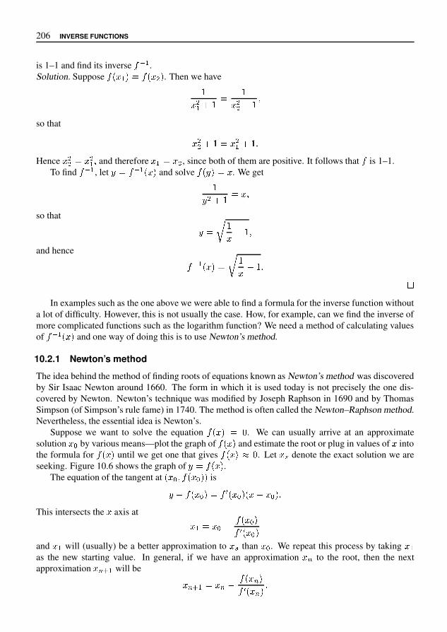
206 INVERSE FUNCTIONS
is 1–1 and find its inverse � � � .Solution. Suppose � � � � � � � � � � . Then we have � � � � � �� � �so that
� �� � � � � � �Hence � �� � � � � and therefore � � � � , since both of them are positive. It follows that � is 1–1.
To find � � � , let � � � � � � � and solve � � � � � . We get � � � � �so that
� � � � �
and hence
� � � � � � � � � �
�In examples such as the one above we were able to find a formula for the inverse function without
a lot of difficulty. However, this is not usually the case. How, for example, can we find the inverse ofmore complicated functions such as the logarithm function? We need a method of calculating valuesof � � � � � � and one way of doing this is to use Newton’s method.
10.2.1 Newton’s method
The idea behind the method of finding roots of equations known as Newton’s method was discoveredby Sir Isaac Newton around 1660. The form in which it is used today is not precisely the one dis-covered by Newton. Newton’s technique was modified by Joseph Raphson in 1690 and by ThomasSimpson (of Simpson’s rule fame) in 1740. The method is often called the Newton–Raphson method.Nevertheless, the essential idea is Newton’s.
Suppose we want to solve the equation � � � � " . We can usually arrive at an approximatesolution � $ by various means—plot the graph of � � � � and estimate the root or plug in values of � intothe formula for � � � � until we get one that gives � � � � � " . Let � �
denote the exact solution we areseeking. Figure 10.6 shows the graph of � � � � � .
The equation of the tangent at � � $ � � � � $ � � is
� � � � � $ � � . � � $ � � � � � $ � �This intersects the � axis at � � � $ � � � � $ �� . � � $ �and � � will (usually) be a better approximation to � �
than � $ . We repeat this process by taking � �as the new starting value. In general, if we have an approximation � 5 to the root, then the nextapproximation � 5 6 � will be
� 5 6 � � 5 � � � � 5 �� . � � 5 � �

CALCULATING FUNCTION VALUES FOR INVERSES 207
� �
� �
� �
� � � � ��
�
Figure 10.6: Newton’s method
We thus generate a sequence of values � � � � , which in most cases converges to the root � � .
EXAMPLE 10.6Let’s solve the equation � � � � � � . Since � will be a cube root of 2, we expect it to lie between 1and 2. Newton’s rule for this case is
� � � � � � � � �� � �$ � %�
� � � � � ' �$ � %�
)
Take � � � , ) . as a first guess. Then
� � � � � �� ' �$ � %�
)� , ) � / 0 $
� % � � � � � ' �$ � % �
)� , ) � 0 � / $
� � � � � � % ' �$ � %%
)� , ) � . / / �
� 2 � � � � � ' �$ � %�
)� , ) � . / / � )
The convergence is rapid and we get � )� , ) � . / / � . 4
Our main interest in Newton’s method will be for calculating inverse function values. Suppose weare given a function and that we wish to calculate 5 � � 7 � for some number 7 in the domain of 5 � .We have
� 5 � � 7 � � � 7

208 INVERSE FUNCTIONS
so that
� � � � � � � � � � � �
Hence putting � � � � � � � and solving � � � � � � � for � gives us � � � � � .
EXAMPLE 10.7Let � � � � � � � � � � , � ! � . Determine � � � � " . Notice that � � � is well-defined since � % � � ! �for all � . According to the discussion in the text, we have to solve the equation � � � � " � � for � ,that is, we have to solve � � � � � � � " � � . Newton’s rule for this case is
� / 1 � �" � �/ � �
3 � 4/ � ��
Take � 6 � � as a first guess. Then
� � �" � �6 � �
3 � 46 � �� � � � 8 " 9
�4
�" � �
�� �
3 � 4 �� �
�� � � : ; : � < 8
� � �" � �
4� �
3 � 44
� ��� � � : ; " 3 <
� > �" � �
�� �
3 � 4�� �
�� � � : ; " 3 " ;
� ? �" � �
>� �
3 � 4>� �
�� � � : ; " 3 " ; �
We conclude that � � � � " �� � � : ; " 3 " ; .
10.2.2 The inverse of the logarithm function
We can now apply our knowledge of inverse functions to the logarithm function. Firstly, we note that
@@ �
� A B C � ��
�! � F
since the domain of A B C � is � � F H . Hence A B C � is an increasing function on its domain, whichimplies that it is 1–1. This shows that the A B C function has an inverse. In order to conform with thenotation of Theorem 10.2, let us put � � � � A B C � . Then the inverse of the logarithm function is � � � .By Theorem 10.2 we have
� � � � % � � ��
� % � � � � � � � (10.4)
Now � % � � � � I � , so the above equation can be written
� � � � % � � ��
� I � � � � �
� � � � � �

CALCULATING FUNCTION VALUES FOR INVERSES 209
Hence the inverse of the log function is its own derivative. In other words
�� �
� � � � � � � � � �
� �
Furthermore, � � � � � � , so that � � � � � � . Hence � � � � � � � �
� � � satisfies the initial valueproblem
� � � � � � � � � � � � � � � � � �
whose solution we know to be the exponential function. We would like to conclude that
� � � � � � � & ' � (10.5)
This is in fact true, but it is important to realise that we are using a result from the theory of differentialequations which states that initial value problems such as (10.5) have one and only one solution. Thefact that exponentials and logarithms are inverses of each other proves the following theorem.
THEOREM 10.4We have & � � � ' � � for all � ) � .
The relationship between the logarithmic and exponential functions is shown graphically in Fig-ure 10.7.
� � � � � �
� � & '
1 2 3 4
1
2
3
4
Figure 10.7: & ' as the inverse of � � � �
10.2.3 Computing the exponential function
We have already computed & ' for various values of � using infinite series. We can now calculate it ina totally different way. Recall (page 207) that we can compute inverse functions by using Newton’smethod. Since the exponential function is the inverse of the logarithmic function, we can compute & 'by solving the equation
� � � � & ' � 2 � � � �
Let’s try computing � � � � � , so that we have to solve � � � � 2 � � � for � . Using Figure 10.7, weguess � = � @ . Then using
� A B � � A 2� � � � A 2 �
� C � A�

210 INVERSE FUNCTIONS
we get
� � � � � � � � � � �� � � �
�� � � � � � � �
� � � � � � � � � � �� � � �
�� � � � � � � �
� � � � � � � � � �� � � �
�� � � � � ! � !
� " � � � � � � �� � �
�� � � � � ! � ! �
Thus # �� � � � � ! � ! . If we are to be totally honest in the above calculation and not use built-in functionsin calculators and/or computers, then the values � � , � � � � � � � � , � � � � � � � � and � � � � � ! � ! willhave to be calculated by a method such as Simpson’s rule using the definition of the logarithm as anintegral. Truly a heroic calculation!
The calculations of # by power series and by Simpson’s rule and inverse functions are completelydifferent, but produce exactly the same result. This is not an obvious fact. Rather, it is a consequenceof the theory we have developed.
10.2.4 The air pressure problem
In Chapter 6 we solved the initial value problem
� ' ( * , � � ( * , 0 � ( 3 , � � �by using infinite series. Using the material developed in this chapter, we can now solve it by a quitedifferent method. We have
� ' ( * ,� ( * , � � 0
so that
77 * ( � � , � � �
Hence
� � � * : � 0
for some constant � . Thus
� � � ; � ( * : � ,� # = > �
� ? # = 0where
? � # � . Using the initial condition � ( 3 , � � � , we find? � � � . Consequently, the solution to
the initial value problem above is� � � � # = 0
as we have previously shown.

CALCULATING FUNCTION VALUES FOR INVERSES 211
EXAMPLE 10.8When light passes vertically through a transparent substance, the rate at which the intensity � � � �decreases is proportional to � � � � , where � represents the distance (in metres) travelled by the light. Inclear seawater, it is found that the intensity of light 1 m below the surface is 25% of the intensity � � atthe surface. What is the light intensity 5 m below the surface?Solution. We can write � � � � � � � � �where � is a constant. This equation can be integrated to give
� � � � � � � � � � � � �� � � � � � � � � �where
� � � � . We have to find both�
and � from the given information and then use these values tofind � � � � . Firstly, we put � � ! , � � � � to get
� � � � , so that
� � � � � � � %Next, put � � ' , � � ! % ( � � � to get ! % ( � � � � � � � � %Hence � � � ! % ( � . Finally, if � � � , then
� � � � � , �� � � � � � � ,� � � / � ! % ( � � ,%� ! % ! ! ' � � �
or about 0.1% of the surface value.1 1We conclude this section by proving two results which make use of the inverse function rela-
tionships between exponentials and logarithms. First we prove a theorem on the convergence of thesequence 2 � ' � 6 8 9 � ; < .
THEOREM 10.5 The sequence �= ' � 69 > ; �
converges to � ? . In particular, the sequence
@ A ' � '9 C ; Econverges to � .
1This value may seem to run counter to what we expect from experience, but it only indicates that the human eye is ableto function effectively over a vast range in light intensity. For example, the brightness of moonlight from a full moon is (onaverage) 0.0002% of the brightness of sunlight.

212 INVERSE FUNCTIONS
We have
� � � � � � �
� � � � � � � �
� � � � � � � � � � � � � �
� � � � � � � � � � � � � � � � �
The thing to notice is that, as " , the limit of the term
� � � � � � � � � � � � � �
is just� � � $ � � � � �
Thus
� � � � � � �
� � � � ) * +
so that
� � � �
� ) * �The second result is the definition of irrational powers of a real number. Rational powers such as
- / and - / � 0 can be defined using ordinary arithmetic, but this is not the case for irrational powers suchas - / . If 1 is any rational number, then by Theorem 10.4, we see that
2 ) � � � 4 � ) 4 � � � (10.6)
Equation (10.6) holds for all rational numbers 1 . We now define 2 * for all , rational or irrational, by
2 * ) 4 � � � * � (10.7)
We call 2 * the general exponential function.
EXAMPLE 10.9Find 6 $ � � if 6 � � * ; < .Solution. We write
� � � 6 � � � � � � * ; < � � � � � � � � �
DIfferentiating both sides gives
6 $ � �6 � � � �
� � � �
� � � � � � � �

CALCULATING FUNCTION VALUES FOR INVERSES 213
Consequently,
� � � � � � � � � � � �� � � � � � � � � � � � � �� � � � � � � �
EXERCISES 10.2
Simplify the following:
1. � � � � � 2. � � � � � � � 3. � � � � �4. � ! � � � � 5. � � ! � � � � 6. � � � � � � � �
Differentiate the following functions:
7. � � � � � � 8. � � � � � � �9. � � � � � $ � ' � � � 10. � � � � ) � �
11. � � � � � � � � � � � �Apply Newton’s method in Exercises 12–17 to find a root of the given equation in the indicatedinterval.
12. � * ) - / 1 � / ) 4 13. � 5 * ) - / 1 � / ) 414. � * $ � ' � - / 1 - / ) 4 15. � 5 * ; � � � / 1 � / > 416. ' A B � * � / 1 - / ) 4 17. � * ) � * D - / 1 � / > 418. Use Newton’s method to find a value of � for which� �E F � � F G F �) �
In Exercises 19–22, apply Newton’s method to find the value of � ! � � H � at the given point H .
19. � � � � � 5 / H ) 20. � � � � � � / H )21. � � � � � B � / H > 22. � � � � ' A B � / � N 1 - / � 4 / H - � D23. The ancient Babylonians discovered a way of extracting square roots about 4000 years ago. In
modern notation, their method of finding Q H was to make an initial guess � for Q H and thento take the average of � and H R � as a better guess for Q H . This process was repeated until thedesired accuracy was reached. Use this method to evaluate Q S to 4 decimal places.
24. Show that the Babylonian method in the above example is equivalent to using Newton’s methodon the equation � * H - .
25. A bacteria culture increases by a factor of 6 in 10 hours. How long did it take the number ofbacteria to double?

214 INVERSE FUNCTIONS
26. In 1987, the world’s population was 5 billion. At that time the population was increasing at arate of 380 000 people per day. When would the world’s population be expected to double? Totriple?
27. Radioactive elements decay at a rate proportional to the amount of the element present. Supposea sample of a radioactive element Ra � � � decays to 58% of its original amount after 3 days.
(a) How long does it take for the sample to decay to half of its original value? This is calledthe half-life of the element.
(b) How long does it take for the sample to decay to 20% of its original value?
Atmospheric air contains carbon, almost all of it in the form of carbon dioxide. Most of the at-mospheric carbon occurs as C � � , but there is a small percentage of radioactive carbon (C � � ). Thisradioactive carbon decays with a half life of 5600 years. However, the ratio of C � � to C � � in theatmosphere remains approximately constant, because the C � � is continually replenished by the actionof cosmic rays on nitrogen in the upper atmosphere. Living organisms absorb both the C � � and theC � � and the ratios of these substances in a living organism is the same as in the atmosphere. Once theorganism dies, the C � � decays and is not replaced, so that the ratio of C � � to C � � changes with timeand this ratio can give an indication of the time since death. This is the basis of carbon dating.
28. A bone excavated from an archeological site is found to contain 1% of the original amount ofC � � . Determine the age of the bone.
29. Assume that the temperature of a cup of coffee obeys Newton’s law of cooling. Suppose thecoffee has a temperature of 95 � C when freshly poured and has cooled to 90 � C one minute later.If the room temperature is 25 � C, determine when the coffee will have cooled to 50 � C.
30. A body at a temperature of 32 � C is discovered at midnight in a room of temperature 25 � C. Thebody is speedily taken to the morgue where the temperature is kept at 4 � C. After one hour, thetemperature of the body has fallen to 25 � C. Estimate the time of death.
10.3 THE OSCILLATION PROBLEM AGAINIn Chapter 7 we solved the differential equation
� � � � � � � � � � � � � � � � � � � (10.8)
by means of infinite series. We will now solve it using some of the ideas in this and the previouschapter. We begin by expressing the left hand side of equation (10.8) as a first order derivative. Thetrick in doing this is to multiply the equation by � � . This gives
� � � � � � � � � � �Using the chain rule, we find
�� �
� �� � � � � � �� ! # � � � � � � � � � �and that �
� �� �� � � �� ! # � � � � � � �
then the above equation can be written
�� �
� �� � � � � � � �� � � �

THE OSCILLATION PROBLEM AGAIN 215
and so�� � � � � � � �� � � � � (10.9)
where � is a constant.This last equation has a physical interpretation, which is disguised by the way it has been written.
If we take the differential equation
� � � � � � �for the particle of mass on a spring with spring constant � , the above condition becomes
�� � � � � � � �� � � � � � � (10.10)
This says that the quantity on the left hand side is constant throughout the motion. The constantis called the energy and so we can say that the energy is conserved in the motion. The first termis the kinetic energy of the particle while the second is its potential energy . The left hand side ofequation (10.10) is the total energy of the particle. During motion, energy is changing from one formto the other, but the total energy is constant. This statement assumes that there is no friction in themotion.
By using the initial conditions � � � � � and � � � � � � in equation (10.9), we find � �� and so
� � � � � � � � � �This gives us two possibilities:
� � ! " � $ � � �To decide which of these to take, we use the initial conditions again. Since � � � � � ' � , we discard thenegative sign. Hence
� � " � $ � � �which we write as �
" � $ � �* �
* + � � (10.11)
Following our method in the last chapter, we define a function-
whose derivative satisfies
- � � � � �" � $ � � �
Then equation (10.11) becomes ** + .
- � � � + � � 0 �and hence
- � � � + � � + � 5 , for some constant 5 . The initial condition � � � � � allows us to find5 - � � � , so the solution is - � � � + � � + � - � � � �All that remains is to find
-. We might expect to find an algebraic function for
-, but this turns out
not to be possible, so we to use the device we developed in the previous chapter and define-
in termsof an integral. We define - � ; �
� == � �
> � $ ? � * ? �

216 INVERSE FUNCTIONS
Here � � can be any constant. A judicious choice simplifies things. If � � � � , then � � � and the
above solution becomes � � � � � (10.12)
with � ��
��
�� � � !
" � � � & � & � )
The restriction � � & � & � is necessary because the integrand (that is, the function being integrated)has vertical asymptotes at � . � .
We already know from Chapter 7 that the solution � � of the initial value problem (10.8) is� � � 1 2 3 � , so that we can write equation (10.12) as
1 2 3 � � � ) (10.13)
A function
which has an inverse 4 5 satisfies the equation
4 5 � � � for all � in the rangeof
, and so equation (10.13) suggests that we write
4 5 � � 1 2 3 � , or equivalently, that � �
1 2 3 4 5 � . However, we should not be too hasty in concluding that 4 5 � � 1 2 3 � . A function and its
inverse are both 1–1 functions and certainly 1 2 3 � is not a 1–1 function. What is true though, is thata suitable restriction of 1 2 3 � will be 1–1 and it is this restricted function that we will have to identifywith
4 5 � . Since � � � , we must have
4 5 � � � and so it is the restriction of 1 2 3 � to theinterval ; � < = ? � < = ? B which has to be identified with
4 5 � .We can also show directly from the definition of
and the use of Theorem 10.2 that
4 5 satisfiesthe initial value problem (10.8). As an exercise, you should show that
is 1–1. Consequently,
has
an inverse 4 5 . For ease of notation let
4 5 � C . The derivative of
is given by
D � � �� � � � !
)
From Theorem 10.2, the derivative of the inverse is
C D � � � D C � � �
� = G � � ; C � B !� G � � ; C � B ! )
Then, by the chain rule
C D D � � � C � C D � G � � ; C � B !
� � C � )
Also, � � � , so C � � � and from the above equation for C D � ,
C D � � G � � ; C � B ! � � )
Putting all this together, we see that C satifies the initial value problem
C D D L C � � � C � � � � C D � � � )

THE OSCILLATION PROBLEM AGAIN 217
Hence, as before, � � � � � � � � � � � � � � � ��
� � � ��
� �
The function� � � � is the inverse of � � � � and is called the inverse sine function. The function
�has
domain � � � � � " and range � � � # � � � # � " and is denoted by � � � � � ' . This terminology is not strictlycorrect:
� � � � is not the inverse of � � � � , it is the inverse of the restriction of � � � � to the domain� � � # � � � # � " . However, this notation is well established and the alternative is too clumsy in use.
What more can we say about the properties of the function�
? We begin by plotting its graphusing Mathematica. The basic command is
Plot[Evaluate[Integrate[1/Sqrt[1-tˆ2],{t,0,x}]],{x,-1,1}]
We have restricted ' to the domain � � � � � " of�
. To get a nicer looking plot, try the followinginstruction.
Plot[Evaluate[Integrate[1/Sqrt[1-tˆ2],{t,0,x}]],{x,-1,1},PlotStyle->RGBColor[1,0,0],AspectRatio->Automatic,Ticks->{{-1,1},{-1.5,-1,-.5,.5,1,1.5}}]
The graph is shown in Figure 10.8.
-1 1
-1.5
-1
-0.5
0.5
1
1.5
Figure 10.8: A Mathematica plot of the graph of�
The plot suggests that� � � � � � � + and
� � � � � � � � � + . We have shown that the exact values are� � � � � # � and� � � � � � � # � . Clearly
� � . � . from the way we have defined�
. Also, by theFundamental Theorem of the Calculus,
� 1 � � � �3 � � � 5
is always positive and so�
is an increasing function. The second derivative is
� 1 1 � � � �� � � � 5 � 6 � 5
and hence there is a point of inflexion at � . .
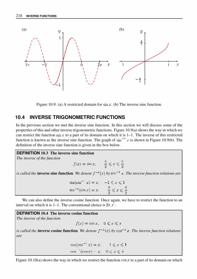
218 INVERSE FUNCTIONS
(a) (b)
�
�
�� �
�
�
� �
�
� � � �
1
� �
�
�
Figure 10.9: (a) A restricted domain for � � . (b) The inverse sine function.
10.4 INVERSE TRIGONOMETRIC FUNCTIONSIn the previous section we met the inverse sine function. In this section we will discuss some of theproperties of this and other inverse trigonometric functions. Figure 10.9(a) shows the way in which wecan restrict the function � � to a part of its domain on which it is 1–1. The inverse of this restrictedfunction is known as the inverse sine function . The graph of � � � � is shown in Figure 10.9(b). Thedefinition of the inverse sine function is given in the box below.
DEFINITION 10.3 The inverse sine functionThe inverse of the function
� � � � � � � � �
� � � �
�is called the inverse sine function. We denote � � � � � � by � � � � . The inverse function relations are
� � � � � � � � � � � � � � � � � � � � � � � � � � �
� � � �
�
We can also define the inverse cosine function. Once again, we have to restrict the function to aninterval on which it is 1–1. The conventional choice is & ' � ) .DEFINITION 10.4 The inverse cosine functionThe inverse of the function
� � � � � * , � � ' � � �
is called the inverse cosine function. We denote � � � � � � by * , � � � . The inverse function relationsare
* , � * , � � � � � � � � � � � � �* , � � � * , � � � � � ' � � �
Figure 10.10(a) shows the way in which we restrict the function * , � to a part of its domain on which
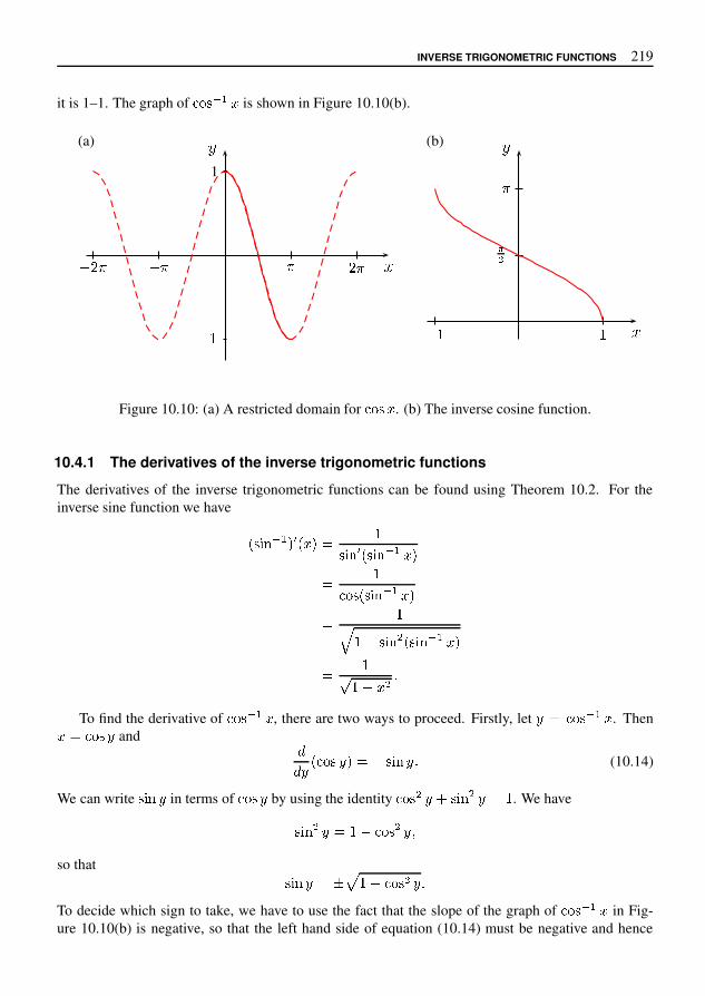
INVERSE TRIGONOMETRIC FUNCTIONS 219
it is 1–1. The graph of � � � � � � is shown in Figure 10.10(b).
(a) (b)
�� �
�
�
�� � � � �� � �
1
� �
Figure 10.10: (a) A restricted domain for � � � � . (b) The inverse cosine function.
10.4.1 The derivatives of the inverse trigonometric functions
The derivatives of the inverse trigonometric functions can be found using Theorem 10.2. For theinverse sine function we have
� � � � � � � � � � � � �� � � � � � � � � � � �
� �� � � � � � � � � � �
� ��� � � � � � � � � � � � � �
� �! � � � �
#
To find the derivative of � � � � � � , there are two ways to proceed. Firstly, let $ � � � � � � � . Then� � � � � $ and
)) $ � � � � $ � � � � � � $ # (10.14)
We can write � � � $ in terms of � � � $ by using the identity � � � � $ 1 � � � � $ � � . We have
� � � � $ � � � � � � � $ 5so that
� � � $ � 8 9 � � � � � � $ #To decide which sign to take, we have to use the fact that the slope of the graph of � � � � � � in Fig-ure 10.10(b) is negative, so that the left hand side of equation (10.14) must be negative and hence

220 INVERSE FUNCTIONS
� � � � must be positive. We take � � � � � � � � � � . Then
�� � � � � � � � � � � � � �� � � � � �
Since � �� � � � � �� � �we have �� � � � � ! � � � � $ � � � �
Alternatively, we can use Theorem 10.2 directly:
� � � ! � % � � � � � � % � � � ! � �� � � � � � � � ! � �� �
� � � � � � � ! � �� � $ � � � �
EXAMPLE 10.10By differentiating � � � ! � * � � ! � �show that � � � ! � * � � ! � is a constant. Hence deduce that
� � � ! � * � � ! � � ./ �
Solution. We have
�� � � � � � ! � * � � ! � � � $ � � � * 2 � $ � � � 4� 6 �Hence � � � ! � * � � ! � � � �where � is a constant. Put � � 6 . Then
� � � � � ! 6 * � � ! 6 � ./ �
so that � � � ! � * � � ! � � ./ �
This result is the reason for the co-terminology for trigonometric functions. The inverse of a functionand its co-function sum to . ; / . Thus each has the same derivative apart from a sign.
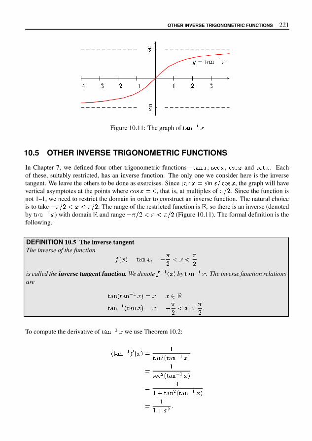
OTHER INVERSE TRIGONOMETRIC FUNCTIONS 221
� � �� �� �� ��
�
� �
� � � � � � �
Figure 10.11: The graph of � � � � � �
10.5 OTHER INVERSE TRIGONOMETRIC FUNCTIONS
In Chapter 7, we defined four other trigonometric functions— � � � � , � � � � , � � � � and � � � � . Eachof these, suitably restricted, has an inverse function. The only one we consider here is the inversetangent. We leave the others to be done as exercises. Since � � � � � " � � # � � � � , the graph will havevertical asymptotes at the points where � � � � ) , that is, at multiples of * # � . Since the function isnot 1–1, we need to restrict the domain in order to construct an inverse function. The natural choiceis to take � * # � , � , * # � . The range of the restricted function is . , so there is an inverse (denotedby � � � � � � ) with domain . and range � * # � , � , * # � (Figure 10.11). The formal definition is thefollowing.
DEFINITION 10.5 The inverse tangentThe inverse of the function
1 2 � 4 � � � � 7 �*
�, � ,
*
�is called the inverse tangent function. We denote 1 � � 2 � 4 by � � � � � � . The inverse function relationsare
� � � 2 � � � � � � 4 � 7 � : .
� � � � � 2 � � � � 4 � 7 �*
�, � ,
*
�<
To compute the derivative of � � � � � � we use Theorem 10.2:
2 � � � � � 4 = 2 � 4 �
� � � = 2 � � � � � � 4
�
� � � 2 � � � � � � 4
�
� @ � � � 2 � � � � � � 4
�
� @ � <

222 INVERSE FUNCTIONS
10.5.1 Computing inverse trigonometric functions
Apart from a few special angles, we have to resort to numerical methods, such as Newton’s method tocompute values of the inverse trigonometric functions. To compute a value of � � � � � � , for instance,we have to solve the equation � � � � � for the value .
EXAMPLE 10.11Compute � � � � � � to 4 decimal places.Solution. Put � � � � � � � � . Then � � � � � � . We put � � � � � � � � � � � and use Newton’s method inthe form
� � � � � � � �� � � � �
� � � � � �
We know that � � � � " # % � � ( , so take as a starting value something a bit bigger than " # % , say � * � ( .Then
� � � � * �� � � � * � �
� � 0 1 � * � ( ( � 3 �
� 1 � � � �� � � � � � �
� � 0 1 � �
� ( ( 5 6 ( 8
� 9 � � 1 �� � � � 1 � �
� � 0 1 � 1
� ( ( 5 : ( ;
� < � � 9 �� � � � 9 � �
� � 0 1 � 9
� ( ( 5 : ( ;
We conclude � � � � � � � ( ( 5 : ( One minor point: How do we calculate the values of � � � � and� � 0 � ? In principle, we have to use infinite series. Of course, nobody would routinely calculate thesefunctions in such a laborious fashion, since they are built into any reasonable calculating device. Infact, so are the values of � � � � � � . However, the method described above is essentially that used bythe calculator, which does not have some mysterious method of its own for doing the calculation. Thepoint of this discussion is not to give practical methods for calculating function values, but rather tolay bare the processes which have to be taken into account when designing algorithms for calculatorsand computers. These functions are built into the calculating device precisely because they arise in alarge number of applications.
10.5.2 CONCLUSIONS
The significance of the inverse trigonometric functions really lies in their derivatives. The derivativeof a trigonometric function is another trigonometric function, but this is not true of the inverse trigono-metric functions. Our discussion in this chapter yields two results that we could not have obtained inother ways. These are �
(= ( � � 1
? � � � � � � � � A (10.15)
and �(
( A � 1? � � � � � � � � A (10.16)
These integrals arise in many problems. As we have already seen, the first arises in oscillationproblems when we use energy methods to find the solution.

OTHER INVERSE TRIGONOMETRIC FUNCTIONS 223
EXERCISES 10.5
Determine the exact value of the following:
1. � � � � � � 2. � � � � � 3. � � � � � � 4. � � � � � � � 5. � � � � � � � �� � � 6. � � � � � � � � � �7. � � � � � � � � � � � � � � � 8. � � � � � � � � � � � 9. � � � � � � � � � � �
10. � � � � � � � � 11. � � � � � � � � # � � 12. � � � � � � � � � �If $ & � , calculate the following:
13. � � � � � � � � $ � 14. � � � � � � � � � $ � 15. � � � � � � � � � $ �If � + $ + � , calculate the following:
16. � � � � � � � � $ � 17. � � � � � � � � � $ � 18. � � � � � � � � � $ �19. � � � � � � � $ � 20. � � � � � � � � � $ � 21. � � � � � � � � � $ �
Differentiate the following functions:
22. . � $ � 2 � � � � � � $ � � 23. . � $ � 2 � � � � � 4 �$ 524. . � $ � 2 6 7 � � � � � $ 25. 8 2 � � � � � � � � $ �26. 8 2 $� ; $ � � � � � $ � � 27. 8 2 > ? $ A � � � � � � $ � �28. . � D � 2 � � � � > � D 29. . � $ � 2 � � � � � � $ 7 �30. Differentiate
. � $ � 2 � � � � 4 $ A FG 5 HHence evaluate the integral � I $
> G � $ A F � H31. Differentiate
. � $ � 2 �G � � � � � 4 $ A FG 5 HHence evaluate the integral � I $G A � $ A F � H

This page intentionally left blank

CHAPTER 11HYPERBOLIC FUNCTIONS
Much of this book has been about the need to introduce functions in order to solve particular problems.The collection of functions we have had to introduce includes algebraic formulas, roots, exponentialand logarithmic functions, trigonometric functions and inverse trigonometric functions. These func-tions, together with all combinations of them, are called elementary functions. The word elementaryis used here in its sense of fundamental or basic, not in the sense of easy. Indeed, as we have seen,there is nothing particularly easy about most of these functions. These functions provide solutions toproblems such as projectile motion, growth and decay and oscillation problems, but there are prob-lems for which these functions are insufficient to provide a solution. The circular motion in the Towerof Terror provides such an example and we shall consider it in Chapter 13. As well as the elemen-tary functions we have already considered, there is another group of elementary functions which playa sufficiently important role in many problems to have been given specific names. These are thehyperbolic functions and their inverses.
11.1 HYPERBOLIC FUNCTIONSThe hyperbolic functions are defined as certain combinations of exponential functions. If you thinkabout the links between complex exponential functions and the trigonometric functions, you willnot be surprised to discover that the hyperbolic functions have many properties which are similar totrigonometric functions.
To motivate the definitions let us consider the equation � � � � � � , which is an example ofundamped simple harmonic motion. Its auxiliary equation is � � � � � with roots � � � � . In realform, the solution is � � � � � � � � � � � � � " (11.1)
which we can write in complex form as as
� � � # $ � � � $ & � �
' ( � � # $ � � ) $ & � �
' � ( + (11.2)
Now let’s keep this example in mind and consider the case
� � � ) � � +The auxiliary equation is � � ) � � with roots � � � � , so the solution is
� � 1 $ � � 2 $ & � +
226 HYPERBOLIC FUNCTIONS
We can regroup the exponential terms in a similar way to that of equation (11.2) by rewriting it asfollows:
� � � �� � �
� � � � � � �
� � � �
� � �� � �
� � � � � � �
� � � � � � �� � �
� � � � � � � �
� � �
� � � � � � � � � � � �
� � � � � � � � � � � � �
� � � � � � � � � �
� � � � � � � � � �
� (11.3)
where� � � �
and� � � �
. There is a marked similarity between the form of this last resultand equation (11.2). We give names to the two combinations of exponential functions occurring inequation (11.3) by defining
� � � � � � � � � � � ��
� " # � � � � � � � � �� %
Then the solution (11.3) becomes
� � � � � � � � � � � " # � � % (11.4)
The function � � � � � is called the hyperbolic cosine of � , while � " # � � is called the hyperbolic sine of� . They are often pronounced as cosh and shine (or sinch by Americans). The similarity betweenthe form of equation (11.4) and that of equation (11.1) is obvious, but this is simply because ofthe notation. However, this notation has been chosen for a reason. It turns out that there are manysimilarities between the trigonometric functions and the hyperbolic functions, some of which we shallexplore below.
EXAMPLE 11.1We consider a case of strongly damped motion given by the equation
� * * � + � * � - � � / %The auxiliary equation is 1 2 � + 1 � - � / with roots 1 � � 7 8 9 : , so the solution is
� � � � ; � � � � � < � � � � � < � � %We can express this in terms of hyperbolic functions by writing
� � � � ; � � � � � = � � < � � � � � < �
> � � � � = � � < � � � � � < �
> �� � � ; � � � � < � � � � � < �
� � � � � � < � � � � � < �� � ?
� � � ; � � � � � � � 9 : � � � � " # � 9 : � � %where
� � � � and
� � � � . B

PROPERTIES OF THE HYPERBOLIC FUNCTIONS 227
In general, if the auxiliary equation of the differential equation
� � � � � � � � � � � � has real roots � �
�, then the solution can be expressed in the form
� � � � � � � � � � � � � ��
� � � ! " ��
� � # (11.5)
EXAMPLE 11.2Solve the equation
� � � $ & � � #The auxiliary equation is * + $ & � ; it has roots � - . The general solution is therefore
� � � � � � � - � � � ! " � - � # 1By analogy with the trigonometric functions, we define four other hyperbolic functions. These are
� " � 4 � � ! " � 4� � � � 4 7 � � � 4 � 9
� " � 4sech 4 � 9
� � � � 4 7 csch 4 � 9� ! " � 4 #
Since the hyperbolic functions are combinations of exponential functions, we could still do all ofthe problems in this book without introducing them. However, they are a very useful conveniencein many circumstances and we shall use them as the need arises. There is a simple occcurrence ofthe hyperbolic cosine that we see almost every day. If a heavy cable such as a power line is strungbetween two points, the curve it hangs in will be a hyperbolic cosine.
EXERCISES 11.1
Find general solutions of the differential equations in exercises 1–4 in terms of the hyperbolic sineand cosine functions.
1. � � � $ - � � 2. � � � $ < � � 3. � � � � > � � � ? � � 4. 4 � � $ - 4 � $ - 4 � 5. Find general solutions of the differential equations in exercises 1–4 in terms of exponential func-
tions. Verify that the two sets of answers you have are equivalent.
11.2 PROPERTIES OF THE HYPERBOLIC FUNCTIONSIt follows from the definitions that � � � � � 9 and � ! " � � . These are the only values of thesefunctions which can be computed exactly. The graphs can be plotted from a knowledge of the graphsof � C and � D C . They are shown in Figure 11.1.
The derivatives of these functions show a similarity to those of the trigonometric functions. Forthe hyperbolic cosine, we have
EE 4 � � � � � 4 � � 9
-E
E 4 � � C � � D C �� 9
- � � C $ � D C �� � ! " � 4 #
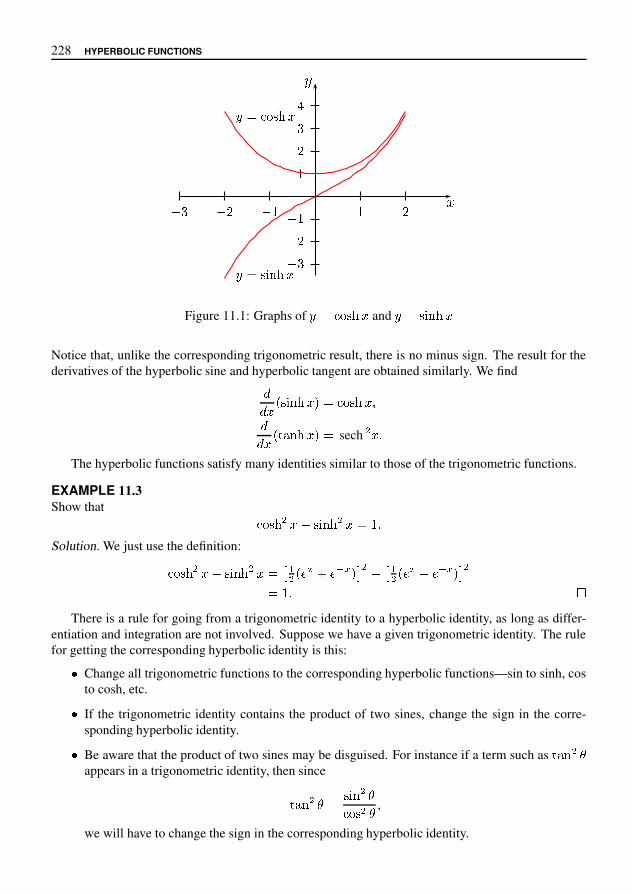
228 HYPERBOLIC FUNCTIONS
�
�
� � � � �
� � � � � �
� �� �� �� �
��
��
� �� �� �
Figure 11.1: Graphs of � � � � � � and � � � � �
Notice that, unlike the corresponding trigonometric result, there is no minus sign. The result for thederivatives of the hyperbolic sine and hyperbolic tangent are obtained similarly. We find
�� � � � � � � � � � � $
�� � � � � � � � sech & � '
The hyperbolic functions satisfy many identities similar to those of the trigonometric functions.
EXAMPLE 11.3Show that
� � � & � � � � & � � � 'Solution. We just use the definition:
� � � & � � � � & � � ,& � - . / - 1 . � & � ,& � - . � - 1 . � &� � ' 3
There is a rule for going from a trigonometric identity to a hyperbolic identity, as long as differ-entiation and integration are not involved. Suppose we have a given trigonometric identity. The rulefor getting the corresponding hyperbolic identity is this:
4 Change all trigonometric functions to the corresponding hyperbolic functions—sin to sinh, costo cosh, etc.
4 If the trigonometric identity contains the product of two sines, change the sign in the corre-sponding hyperbolic identity.
4 Be aware that the product of two sines may be disguised. For instance if a term such as � � & appears in a trigonometric identity, then since
� � & � � &
� � & $
we will have to change the sign in the corresponding hyperbolic identity.

PROPERTIES OF THE HYPERBOLIC FUNCTIONS 229
EXAMPLE 11.4We have
� � � � � � � � � � � � � � � � � � � � � �so the hyperbolic identity is
� � � � � � � � � � �� � � � �
� � � �� � � � �
� �
This rule is a consequence of the fact that both the trigonometric functions and the hyperbolicfunctions can be expressed in exponential form. We have
� � � � � � � � � � �! � � � � � � �
and
� � � � � � � � � � �! �
� � � � � � � � �
So, for example, since
� � � ) � � � � ) � , �we have
� � � � ) � � � � � � � � � � � � ) , �� � � � ) � � � � � � � ) � � , �
Hence
� � � � ) 3 � � � � � ) 3 , �where 3 � � .
We have here another example of results about real functions which are explained by the use ofcomplex numbers. Without complex numbers, the similarity between trigonometric and hyperbolicfunctions would have been inexplicable.
EXERCISES 11.2
Prove the following identities.
1. � � � � 6 , 2. � � � � 6 63. � � � � � � � � � � � � � 4. � � � � � � � � � � � � � �5. � � � � � � � � � � � 6. sech ) � , � � � � ) �7. � � � � � � � 3 � � � � � � � � � � 3 � � � � � � � � � � 38. � � � � � � 3 � � � � � � � � � � 3 � � � � � � � � � 39. � � � � � � � 3 � � � � � � � � � � 3 � � � � � � � � � � 3
10. � � � � ! � ! � � � � � � � � � � 11. � � � � ! � ! � � � � ) � ,

230 HYPERBOLIC FUNCTIONS
12. Show that � � � � � � � � � � � and � � � � � � � � � � � � . Hence show that� � � � � � � � � � � � � � � ! � � � � � ! and � � � � � � � � � � � � � � � ! � � � � � ! for all ! $ & ( .
Find the derivative of the following functions.
13. ) � � � � � � � / � 0 � 14. ) � � � � � � � 215. ) � � � 0/ 3 5 7 � � � � 7 16. ) � � � 3 � � � � � / 17. ) � � � � � � 2 18. ) � � � � � � � � 19. ) � � � � � � 2 20. ) � � � � � � 3 5 21. ) � � � 3 5 sech 22. ) � � � � � � � = 0 >23. ) � � � � � � � � � � � � 24. ) � � � � � � � � � � � 025. ) � � � 3 � 7 � � � � B 7 26. ) � � � / � � � � /27. A body of mass D falls from rest under the action of gravity. It encounters an air resistance
proportional to the square of its velocity. Satisfy yourself that the motion is described by theinitial value problem
D E FE G � D H � J F L $ F � N � � N $where J is a constant which depends on the properties of the particular body.
(a) Show that F � Q D HJ � � � � Q H JD G �is a solution of this initial value problem.
(b) What value does the velocity approach as G gets large? What physical phenomenon isoccurring here?
(c) Let R � G � be the distance of the body from some fixed point at time G . If it is known thatR � N � � R T , find an explicit expression for R .
11.3 INVERSE HYPERBOLIC FUNCTIONSThe hyperbolic functions have inverses which are useful for computing integrals. The function � � � is not 1–1, but if we restrict the domain to U N $ W � , we do get a 1–1 function. The inverse of thisrestricted function is denoted by � � � � X and is called (somewhat incorrectly) the inverse hyperboliccosine function. It has domain U 0 $ W � and range U N $ W � (Figure 11.2).

INVERSE HYPERBOLIC FUNCTIONS 231
� �� �� �� �
�
�
�
�
� �
� � � � � � �� � �
� � � �� �
�
�
�
�
� �
� � � � � � � �
Figure 11.2: Graphs of � � � � � � � � � � and � � � � � � � �
To find the derivative, let " � % � � � � � for � � � . Then
( " � % � * + � � - � � � � . � � � �
since � * + � � � � .The domain of the inverse function is 2 � � 4 % , so for � 6 � we have
88 � " � � � � � � � % " � � % ( " � %
� ( " � � � %
�� * + � " � � � %
��� � � � . " � � � % � �
��� � � � . " � � � � � � � % � �
�< � . � � =
We have the pair of results
88 � " � � � � � � � % �
< � . � � ��
�< � . � � 8 � � � � � � � � @ � = (11.6)
Notice the difference between the integral provided by equation (11.6) and the integral that occurs in

232 HYPERBOLIC FUNCTIONS
connection with the inverse sine (equation (10.15)). The integral��
� � � � � � �
is used on the interval � � � � � � or � � � � , while the integral��
� � � � �� � � � � � � � � ! �
is used on the interval � � � � � .The hyperbolic sine is easier to deal with because it is 1–1, so it has an inverse, denoted � � � � � � ,
with domain and range " (Figure 11.3).
� # $� �� #� $� '
�#
� �� #� $
(
)
* � � � � � � � �
Figure 11.3: The graph of � � � � � � �
The derivative of � � � � � � � is found in a similar manner to that of + - � � � . Let 0 � � � � � � � � .Then
0 6 � � � + - � � �� 8 � ! � � � � � � <
Thus
�� � � � � � � � � � � 0 � � � 6 � �
� �0 6 0 � � � �
� �+ - � � 0 � � � �
� ��� ! � � � � � � � � � � � � �
� �� � ! � �
<

INVERSE HYPERBOLIC FUNCTIONS 233
Thus we have the pair of results
�� � � � � � � � � �
� � � � ��
��
� � � � �� � � � � � � � � � �
� � � �� �� �� �� �� $
�
� �
%
&
' � � � �
Figure 11.4: The graph of � � �
The hyperbolic tangent is also 1–1. It has domain * and range � � � � � (Figure 11.4). It has aninverse, denoted � � � , with domain � � � � � and range * (Figure 11.5).
�� �� �
�
�
� �
� �
%
&
' � � � � �
Figure 11.5: The graph of � � � �
The derivative is found in an analogous way to those of the hyperbolic sine and cosine (Exer-cises 11.3). We have the pair of results
�� � � � � � � � �
� � � ��
��
� � � �� � � � � � � � � �
The inverse trigonometric functions and inverse hyperbolic functions provide a complete set ofintegrals for functions which are reciprocals of quadratics or reciprocals of square roots of quadratics.

234 HYPERBOLIC FUNCTIONS
This is one reason for the importance of these functions. The following list presents the results wehave derived in slightly generalised form useful in applications.
� �� � � � � � � �� � � � � � � � �� �� � � � � � � �� � � � � � � � � �� �� � � � � � � � � � � � � � � �� �� � � � � � � � � � � � � � � � �� �� � � � � � � � � � � � � � � � �
Table 11.1: Indefinite integrals
EXERCISES 11.3
Find the derivatives of the functions in Exercises 1–10.
1. � � � ! � � � � � $ � 2. � � � ! � � � � � � � � � � !3. � � � ! �� � � � � � 4. � � � ! � � � � � � � � � � � � �5. � � � ! � � � � � � � � � � � � ! 6. � � � ! � � � � � � � ! ,7. � � � ! - � � � � � � � � ! 8. � � � ! � � � � � � � � � � !9. � � � ! � � � � � 0 � � � � 10. � � � ! � � � � � 0 � � � �
11. Prove the following two results stated in the text:
�� � � � � � � � � ! �� � � � 3� �� � � � � � � � � � � � � � 4
12. Since the hyperbolic functions can be expressed as exponentials, it is not surprising that theinverse hyperbolic functions can be expressed as logarithms. For the hyperbolic sine we have
� � � � � � - � 5 � � 0 � � � � 6 4(a) Prove this result by showing that the derivatives of the two sides of the equation are equal,
so that the two sides differ by a constant. Show that the constant is zero.
(b) Prove this result by letting 7 � � � � � � and then solving the equation � � � � � 7 for 7 interms of � .
13. Prove the following two results
� � � � � � - � 5 � � 0 � � � � 6 3 � � � � � � �� - � : � � �� � � ; 4
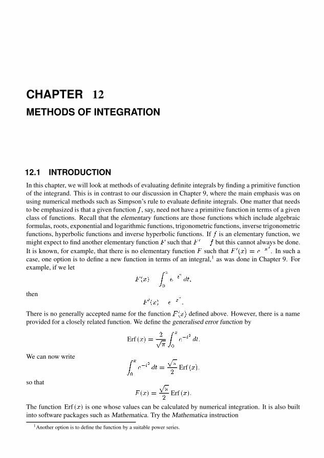
CHAPTER 12METHODS OF INTEGRATION
12.1 INTRODUCTIONIn this chapter, we will look at methods of evaluating definite integrals by finding a primitive functionof the integrand. This is in contrast to our discussion in Chapter 9, where the main emphasis was onusing numerical methods such as Simpson’s rule to evaluate definite integrals. One matter that needsto be emphasized is that a given function � , say, need not have a primitive function in terms of a givenclass of functions. Recall that the elementary functions are those functions which include algebraicformulas, roots, exponential and logarithmic functions, trigonometric functions, inverse trigonometricfunctions, hyperbolic functions and inverse hyperbolic functions. If � is an elementary function, wemight expect to find another elementary function
�such that
� � � � but this cannot always be done.It is known, for example, that there is no elementary function
�such that
� � � � � � � � � . In such acase, one option is to define a new function in terms of an integral,1 as was done in Chapter 9. Forexample, if we let
� � � ��
�� � � � � � � �
then � � � � � � � � � �There is no generally accepted name for the function
� � � defined above. However, there is a nameprovided for a closely related function. We define the generalised error function by
Erf � � � �� �
��
� � � � � � � �
We can now write ��
� � � � � � � � � �� Erf � � �
so that� � � � � �
� Erf � � �
The function Erf � � is one whose values can be calculated by numerical integration. It is also builtinto software packages such as Mathematica. Try the Mathematica instruction
1Another option is to define the function by a suitable power series.

236 METHODS OF INTEGRATION
Plot[Erf[x],{x,-5,5}]to plot its graph. Although not classed as an elementary function, it is conceptually no differentto functions such as � � � � , � � and so on, in that there is a rule of calculation which produces anoutput number from a given input number. The worst that can be said about this function is that it isunfamiliar.
In principle, all definite integrals and functions defined by definite integrals can all be calculatednumerically and, if need be, their graphs plotted without making use of the concept of an indefiniteintegral. However, this is not always necessary or efficient. A simple integral such as � �
� � � � can befar more efficiently evaluated by making use of primitive functions. It is also helpful to know whetherthe functions defined by an integral are new or whether they are known functions in another form. Forexample, the function � � � � �
��
�
� � � � � �
is just another way of writing � � � � � so that�
is not a new function. For these reasons, we needmethods for finding elementary functions for integrals when this is possible. There are also practicalproblems such as the length of a curve, areas, volumes and so on, which can be expressed as definiteintegrals. We will not consider such applications in detail in this book, but we will briefly summarisethem below.
Areas
The area under a curve has already been dealt with in Chapter 9. If � is a given positive function, thearea bounded by the graph, the � axis and the vertical lines � � ! , � � # for ! and # in the domain of
� is$ �
� �� � � � � � � (
Volumes of revolution
Let � be a function such that � � � � * , for ! . � . # . If the graph of � is rotated about the � axis,then a solid is generated. The volume of this solid is
� � 0� �
� 1 � � � � 3 � � � (
The length of a curve
The length of the curve 4 � � � � � from the point � ! 8 � � ! � � to the point � # 8 � � # � � is
�� �
� > � � 1 � @ � � � 3 � � � (
Work
The work
done by a constant force on a body moving in a straight line is the product ofA
, thecomponent of the force in the direction of movement, and � , the total distance moved. Thus � A � (
CALCULATION OF DEFINITE INTEGRALS 237
The work done represents the increase of kinetic energy of the body. For example, for a falling body ofmass � , the force is a constant � � and in falling a distance � the work done is � � � . This representsthe increase in kinetic energy, which is �� � � � , so we have
� � � �� � � � �and hence � � � � . If we take the example of the Tower of Terror, then � � � � m, and hence
� � � m/sec.If the force
�varies, such as in a spring where
� � � � � � , it can be shown that
� � �
!� � � � # � �
where � ' and � ) are the end points of the motion.
12.2 CALCULATION OF DEFINITE INTEGRALSThere are two methods available to compute a definite integral. We can do it numerically and (usually)approximately using a method such as Simpson’s rule. However, if we can find a primitive functionfor the integrand then we can express the definite integral in an exact form in terms of the primitivefunction. We have already considered numerical evaluations in Chapter 9 and in this chapter we wantto concentrate on methods for finding primitives.
There is a very useful result, related to the Fundamental Theorem of the Calculus, which we nowstate.
THEOREM 12.1 Evaluating definite integralsLet * be a continuous function on the interval + ' � ) / and let
�be a primitive function for * . Then� �
! * � � � # � � � ) � 4 � � ' � 7
To prove this result, let�
be any primitive of * . Then� 8 * . Now let
� � � � �
9! * � : � # : �
so that� 8 * . Then
�and
�are both primitives of * and must differ by a constant. Thus
� � � � � � � � > � for all � @ + ' � ) / . Put � ' . Then A � � ' � > � , so that � 4 � � ' � . Hence� � � � � � � � 4 � � ' � �so that � � ) � � � ) � 4 � � ' � �which is to say � �
! * � � � # � � � ) � 4 � � ' � 7
As a matter of notation, we write � � � � � �! for
� � ) � 4 � � ' � .

238 METHODS OF INTEGRATION
EXAMPLE 12.1Since �
� � � � � � � � � � � � � �
we have � ��
� � � � � � � � � � � � � �� (12.1)
� � � � � � � � � � � " #
Notice that it is unnecessary to put the constant � in equation (12.1). If you don’t understand why, tryputting in the � and see what happens. $
The calculation of a definite integral by this method requires us to be able to find an indefiniteintegral among the known functions. There are two ways to do this:
% To make use of a table of integrals. These can range from a small table, such as Table 12.1, tolarge books of tables.
% If a particular indefinite integral is not on our list, we may be able to rewrite it in terms ofintegrals that do appear in the table. This chapter is largely about such methods.
�� & � � �
� & ( )* � -
� � � * 0� -
�-
2 3 � � 3� � �
-2
� � 5 ) �2
� ��-
�� � � 6 � 7 9 � 9 � � � � 0� �
�-
= 2 3 � 3� � � � � � 5 ) �
2� ��
? @ � � � ? @ � ��
-= 2 3 � � 3
� � � � � � � 5 ) �2
� ��� � � � � � � � � � � � �
�-
= � 3 2 3� � � � � � � 5 ) �
2� ��
� � � � � � � � � � � � ��� � 3 � � � � � � � � �
Table 12.1: Indefinite integrals
There are two main methods of transforming integrals into a standard form. Firstly, there aremethods that make use of differentiation formulas and, secondly, we can rewrite the integral by usingalgebraic manipulation or trigonometric identities.

INTEGRATION BY SUBSTITUTION 239
EXERCISES 12.2
Evaluate the following integrals:
1.
� � � �� � � � � � 2.
� � � �� � � � � � � � � �
3.
��
� � � � ! # � � � 4.
��
��
� ! � � �
5.
��
��
& � � � � � 6.
��
� � � � � � �
7.
� �� � � � � � � � � � � 8.
� � � *� � � � ! � � � � � �
9.
��
�
�� � � 10.
� � �� ��
11.
� � � *� , � - � 12.
��
. �/ � � � � ,
where / � � � is the Heaviside function defined in Exercises 2.6.
12.3 INTEGRATION BY SUBSTITUTION
This method is derived from the chain rule. Suppose1
is a primitive for 2 . Then for any differentiablefunction 3 , we have
�
1 3 � � � 6 1 7 3 � � � 3 7 � �6 2 3 � � � 3 7 � � <
Thus �2 3 � � � 3 7 � � � 6 1 3 � � � ! � < (12.2)
This is the rule for integration by substitution . It is possible to use it as it stands, as is done in thefollowing example.
EXAMPLE 12.2Consider �
� � � � � � � � <
If 3 � � 6 � � , then 3 7 � � 6 � � and the integral has the form�� � � 3 � � 3 7 � � � <

240 METHODS OF INTEGRATION
In this example, the function corresponding to � in equation (12.2) is the sine function. Thus � � � � � � and� � � � � � � � . So putting all of this into equation (12.2) gives�
� � � � � � � � � � � � � � � � � � � ! � � � � � # ! � %
&You may find the above example confusing. In fact, there is no need to explicitly identify the
functions�
, � and � in order to use integration by substitution. It is perhaps worthwhile to use theformula once or twice in this way to convince yourself that you understand it and why integration bysubstitution works, but then you should approach such problems as in the next example.
EXAMPLE 12.3In the integral �
' � � � # � �put ) � # , so that � )
� � ' � %Then symbolically write � ) ' � � � . In the integral we now replace � # by ) and ' � � � by � ) to get�
' � � � # � � �
� ) � ) � � � ) ! � � � � � # ! � %
Much easier! Note that after we have made the substitution ) � # , the new integral must not containthe original variable � . &EXAMPLE 12.4/ In the integral �
� 0 1 ! � # � � 4put ) � # ! 1 ( ) � # also works), so that � ) ' � � � and hence � � � 9# � ) . Then theintegral becomes
9#�
: ) � ) 9# < #= ) = � # > ! � 9= � 1 ! � # � = � # ! � %
/ In the integral � � � # � � # � � � 4
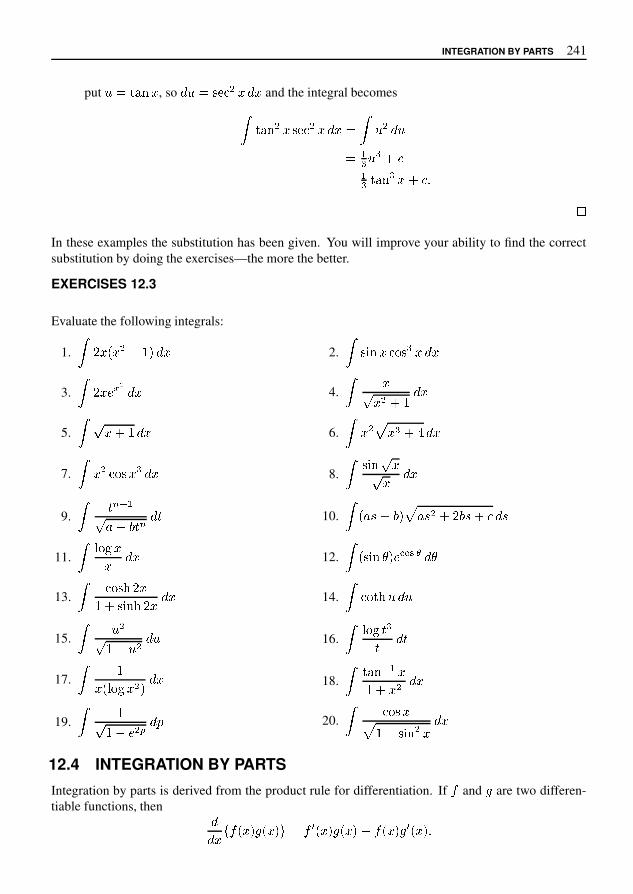
INTEGRATION BY PARTS 241
put � � � � � � , so � � � � � � � � � � and the integral becomes� � � � � � � � � � � � � ��
� � � �� �� � � � � �� � � � � � � �
�In these examples the substitution has been given. You will improve your ability to find the correctsubstitution by doing the exercises—the more the better.
EXERCISES 12.3
Evaluate the following integrals:
1.
�� � � � � � � � � � 2.
�� ! � � � # � � � � �
3.
�� � & ' � � � 4.
� �( � � � � � �
5.
�( � � � � � 6.
�� � + � � � - � �
7.
�� � � # � � � � � 8.
� � ! � ( �( � � �
9.
� / 0 2 �( 3 � 6 / 0 � / 10.
�� 3 9 � 6 � + 3 9 � � � 6 9 � � 9
11.
� = # > �� � � 12.
�� � ! � � � & � � � � �
13.
� � # � � � �� � � ! � � � � � � 14.
�� # � � � � �
15.
� � �( � C � � � � 16.
� = # > / �/ � /
17.
� �� � = # > � � � � � 18.
� � � � 2 � �� � � � � �
19.
� �( � C & � � � H 20.
� � # � �+ � C � ! � � � � �
12.4 INTEGRATION BY PARTSIntegration by parts is derived from the product rule for differentiation. If I and J are two differen-tiable functions, then
�� �
K I � � � J � � � O � I Q � � � J � � � � I � � � J Q � � � �
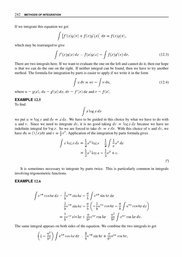
242 METHODS OF INTEGRATION
If we integrate this equation we get�� � � � � � � � � � � � � � � � � � � � � � � � � � � � � �
which may be rearranged to give�� � � � � � � � � � � � � � � � � � �
�� � � � � � � � � � � (12.3)
There are two integrals here. If we want to evaluate the one on the left and cannot do it, then our hopeis that we can do the one on the right. If neither integral can be found, then we have to try anothermethod. The formula for integration by parts is easier to apply if we write it in the form�
� � � � � � ��
� � � � (12.4)
where � � � � � , � � � � � � � � � , � � � � � � � � � � and � � � � � � .
EXAMPLE 12.5To find �
� * + , � � �we put � � * + , � and � � � � � � . We have to be guided in this choice by what we have to do with� and � . Since we need to integrate � � , it is no good taking � � � * + , � � � because we have noindefinite integral for * + , � . So we are forced to take � � � � � � . With this choice of � and � � , wehave � � � � 7 9 � � � � and � � <= � = . Application of the integration by parts formula gives�
� * + , � � � � 7> � = * + , � � 7>� 7� � = � �
� 7> � = * + , � � 7@ � = � � �A
It is sometimes necessary to integrate by parts twice. This is particularly common in integralsinvolving trigonometric functions.
EXAMPLE 12.6
�B C D E + H J � � � � 7J B C D H M N J � � O J
�B C D H M N J � � �
� 7 J B C D H M N J � � O J P � 7J B C D E + H J � � O J�
B C D E + H J � � � R� 7 J B C D H M N J � � OJ = B C D E + H J � � O =J =
�B C D E + H J � � � �
The same integral appears on both sides of the equation. We combine the two integrals to get
P 7 � O =J = R�
B C D E + H J � � � � 7J B C D H M N J � � OJ = B C D E + H J � �

THE METHOD OF PARTIAL FRACTIONS 243
so that�
� � � � � � � � � �
� � � �� � � � � � � �
�� � � �
� � � � � � � �
�The special case � � � " � � in equation (12.3) is often useful. In this case, equation (12.3) becomes�
% � � " � � � � % � � " +
�� % , � � " � � � (12.5)
EXAMPLE 12.7
�- � . � � � � � - � . � +
��
2�
� �
� � - � . � + � � � �
�
EXERCISES 12.4
Evaluate the following integrals:
1.
�� � � � � 2.
�� � � � � � �
3.
�� � � � � � � � 4.
�� � � 9 : � � �
5.
�� � � 9 : � � � 6.
�� � � � � 9 : � � �
7.
�� � � � � < � � � 8.
�� � - � . � � �
9.
�= � � ?
� �� � 10.
�� � � � � � � �
11.
�� � � � 9 : � " � � � 12.
�- � . �
� �� �
13.
�� � � � - � . � � � � � " � � 14.
�� � � - � . � " � � �
12.5 THE METHOD OF PARTIAL FRACTIONSThe previous two methods of integration have been based on differentiation rules. The method ofpartial fractions relies on using algebraic methods to rewrite the integrand in a form which is easier tointegrate.
In order to see where we are going, let’s first consider an example.

244 METHODS OF INTEGRATION
EXAMPLE 12.8It is easily checked that �� � � � � � �� � � � �� � �We will have to consider methods of deriving the right-hand side from the left-hand side, but we won’tworry about it just yet. If we want to find the integral� �� � � � � � � � �we can do it easily by writing
� �� � � � � � � � �
� �� � � � �� � � � � � � � � � � � ! � � � � � � � ! � � �
&Partial fractions are used for functions which are quotients of two polynomials, such as
� � �� � � � � � � � ' � �� � � � � � � � � �� � � � ! � � � � ! � � � � ! or�� � � � ! � � � � � � � ! �
Functions of this type are called rational functions.Let us first consider rational functions where the degree of the numerator is less than the degree
of the denominator. There are two facts about polynomials which we will make use of:
, Any polynomial can be factorised into a product of linear and quadratic factors. In the generalcase this may be difficult and we will only deal with cases where the factorisation has alreadybeen done or is easy.
, The second fact is that once we have factorised the denominator of a rational function, then thefunction can be split into separate fractions, one for each factor. This is called the partial fractiondecomposition of the function. In each fraction the degree of the numerator will be less thanthe degree of the denominator. An example of such a decomposition appears in Example 12.8above.
We will only consider cases where the denominator of a rational function has factors which are alldifferent. In this case, each linear factor - � � / in the denominator will give a fraction0
- � � /in the partial fraction decomposition, where
0is a constant. Each quadratic factor - � � � / � � � gives
a fraction 0 � � 3- � � � / � � �
in the partial fraction decomposition, where0
and3
are constants.

THE METHOD OF PARTIAL FRACTIONS 245
EXAMPLE 12.9Find the partial fraction decomposition of
�� � � � � � � � �
Solution. The form of the partial fraction decomposition is
�� � � � � � � � �
�
� � � ��
� � � �
so all we have to do is find�
and�
. One way to do this is to multiply through by the denominator ofthe left hand side. This gives
� � � � � � � � � � � � � �This has to hold for all values of � , so we can substitute any two values of � to get two equations in�
and�
. Some choices of � involve less work than others. In this case put � � � � to get � � � �and then put � � � � to get � � � � �
. Hence� � � � and
� � � , so
�� � � � � � � � � � �
� � � � �� � � �
EXAMPLE 12.10Find �
!� � � � � � $ � � % � �
Solution. We have!
� � � � � � $ � � ��
� � � �� � � )
� $ � � �
We multiply by the denominator of the left hand side to get
! � � � � $ � � � � � � � ) � � � � �
Putting � � � gives� � � . To find
�and
)we equate coefficients of like powers of � on both
sides of the equation (Theorem 5.1 of Chapter 5). With practice, you should be able to do this withoutexpanding the right hand side completely, but in this example we will give more detail. The aboveequation can be written
! � � � � � � $ � � � � ) � � � � ) �so we have
� � � � . �� � ) � . �� � ) � ! �
We could solve these equations simultaneously for�
,�
and)
, but we already know� � � , so we
quickly find� � � � and
) � � � .

246 METHODS OF INTEGRATION
Now we can return to the integral:� �� � � � � � � � � � ��
� �� � � � � � �� � � � � ��
�� �� � � � � �� � � � �� � � � � �
� � � � � � � � � � � � � � � � � � � ' ( ) � � +,
We have not yet considered the case where the numerator of a rational function has degree greaterthan or equal to the degree of the denominator. The method here is to do a long division and then findthe partial fraction decomposition of the remainder. We illustrate this in the next example.
EXAMPLE 12.11Expand � � - / � - 2 � �� � 3 � �in partial fractions.Solution. On dividing the numerator by the denominator, we find
� � - / � - 2 � �� � 3 � � � � � � �� � 3 � �� � � � �� � � � � � � � � � � �� � �� � 6
where, in the last step, we have used the result in example 12.9. ,The method of partial fractions can be further developed to deal with cases where higher powers
of the linear or quadratic factors appear in the denominator, for example, integrals of the type� �� � � � � � � - � �or � � � �� � � - � � � � � � � � +We won’t go into the details of how to attack these cases by hand, but we will show you how Mathe-matica can be used to find the partial fraction decompositions.
The relevant Mathematica instruction is Apart, so to find the partial fraction decomposition of
�� � � � � � � -we use
Apart[x/((x+1)(2x+1)ˆ3)].
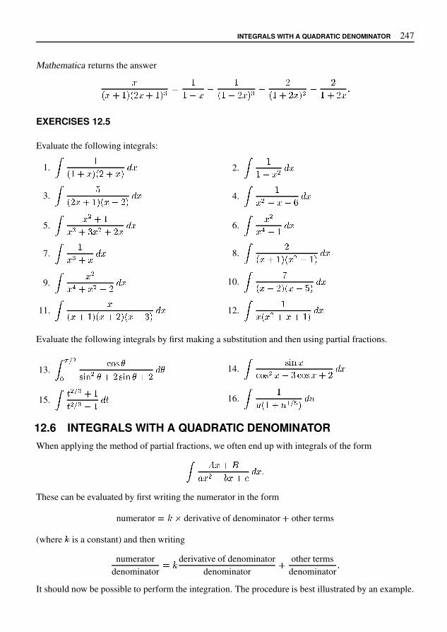
INTEGRALS WITH A QUADRATIC DENOMINATOR 247
Mathematica returns the answer
�� � � � � � � � � � � �
� � � � �� � � � � � � �
� � � � � �� �
� � � � �
EXERCISES 12.5
Evaluate the following integrals:
1.
��
� � � � � � � � � � 2.
��
� � � �� �
3.
��
� � � � � � � � � � � 4.
��
� � � � � ! � �
5.
�� � � �
� � � # � � � � � � � 6.
�� �
� % � � � �
7.
��
� � � � � � 8.
��
� � � � � � � � � � �
9.
�� �
� % � � � � � � � 10.
�'
� � � � � � � � � �
11.
��
� � � � � � � � � � � # � � 12.
��
� � � � � � � � � �
Evaluate the following integrals by first making a substitution and then using partial fractions.
13.
� � � �*
+ , - �- / 0 � � � � - / 0 � � � � �
14.
�- / 0 �
+ , - � � � # + , - � � � � �
15.
�4 � � � � �4 � � � � � � 4 16.
��
5 � � � 5 7 � 8 � 5
12.6 INTEGRALS WITH A QUADRATIC DENOMINATORWhen applying the method of partial fractions, we often end up with integrals of the form� 9 � � :
; � � � < � � � � � �
These can be evaluated by first writing the numerator in the form
numerator � A C derivative of denominator � other terms
(where A is a constant) and then writing
numeratordenominator
� A derivative of denominatordenominator
� other termsdenominator
�
It should now be possible to perform the integration. The procedure is best illustrated by an example.
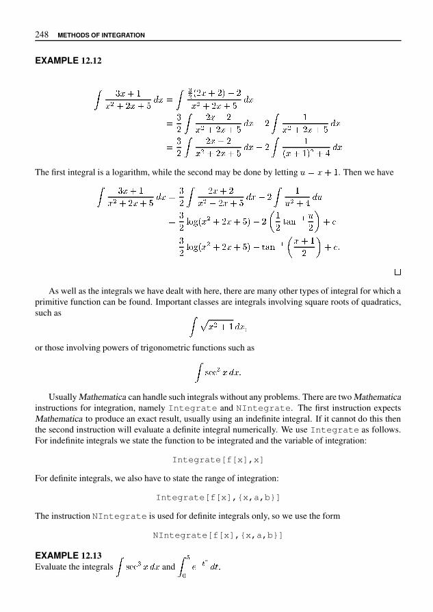
248 METHODS OF INTEGRATION
EXAMPLE 12.12
� � � � �� � � � � � � �� �� � � � � � � � � � � � �
� � � � � � � � � � � � �
� �� � � � � � �� �
� � � � � � � � � � � � �� � � � � � � � �
The first integral is a logarithm, while the second may be done by letting � � � � � . Then we have� � � � �� � � � � � � � � � � � � � � � � � � �
� �� � � � �� � ! " � � � � � � � � � & � � � ' ( ) � * � �� � ! " � � � � � � � � � � � ' ( ) & � � � * � � ,
-As well as the integrals we have dealt with here, there are many other types of integral for which a
primitive function can be found. Important classes are integrals involving square roots of quadratics,such as �
. � � � � � 1or those involving powers of trigonometric functions such as�
2 4 � � � ,Usually Mathematica can handle such integrals without any problems. There are two Mathematica
instructions for integration, namely Integrate and NIntegrate. The first instruction expectsMathematica to produce an exact result, usually using an indefinite integral. If it cannot do this thenthe second instruction will evaluate a definite integral numerically. We use Integrate as follows.For indefinite integrals we state the function to be integrated and the variable of integration:
Integrate[f[x],x]
For definite integrals, we also have to state the range of integration:
Integrate[f[x],{x,a,b}]
The instruction NIntegrate is used for definite integrals only, so we use the form
NIntegrate[f[x],{x,a,b}]
EXAMPLE 12.13Evaluate the integrals
�2 4 � � � and
� 67 8 ( � 9 ,
CONCLUDING REMARKS 249
� To evaluate
�� � � � � � � use
Integrate[(Sec[x])ˆ3,x].
The result given by Mathematica is, after some rearragement of the terms,�� � � � � � �
�� � � � � � � � � � �
�� � � � � � �
�� � � � � � � � � � � �
�� � � � � � �
�� � �
� � � � � � " � � � � � " %� To evaluate � &
' ( ) � � � * ,use
NIntegrate[Eˆ(-tˆ2),{t,0,5}].
The result is � &' ( ) � � � * / % 1 1 2 � � 3 %
512.7 CONCLUDING REMARKSThere are two main reasons for calculating definite integrals in terms of indefinite integrals.
� Generally speaking, it is easier to evaluate definite integrals exactly if we can find a primitiveof the integrand. Many quantities (area, volume, work) can be expressed as definite integrals. Ifwe can compute them exactly by using indefinite integrals, then we do so. Otherwise we haveto use numerical methods to calculate them approximately.
� Many problems require us to define functions in terms of definite integrals and it is often usefulto know whether this defines a new function or is just another way of expressing a knownfunction. For example, the function
6 � � " � 8
' ( ) � � � *cannot be calculated in terms of the functions we have met earlier in this book. This is a factwhich can be proved and it is not just that we are not clever enough to think of a way to do it.Consequently,
6is a new function. On the other hand, the function
� � " � 8
'�
� � * : � *is not a new function. We know that
� � " � � � ) ; � .
250 METHODS OF INTEGRATION
EXERCISES 12.7
Evaluate the following integrals:
1.
��
� � � � � � �� � 2.
��
� � � � � �� �
3.
� � � �
� � � � � � � �� � 4.
�� �
� � � � � � � �� �
5.
�� � � �
� ! � � � � ! � � %� � 6.
� � � &
' � � � ( � � %� �
7.
�� � &
� � � � � � %� � 8.
�& � � �
� � � � � �� �
9.
�� � � �
� ) � � � � �� � 10.
�� � � � �
� � � � � � � � � ! � � �� �
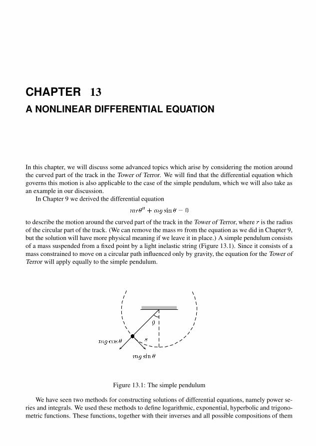
CHAPTER 13A NONLINEAR DIFFERENTIAL EQUATION
In this chapter, we will discuss some advanced topics which arise by considering the motion aroundthe curved part of the track in the Tower of Terror. We will find that the differential equation whichgoverns this motion is also applicable to the case of the simple pendulum, which we will also take asan example in our discussion.
In Chapter 9 we derived the differential equation
�� � � � �
�� � � �
to describe the motion around the curved part of the track in the Tower of Terror, where � is the radiusof the circular part of the track. (We can remove the mass
�from the equation as we did in Chapter 9,
but the solution will have more physical meaning if we leave it in place.) A simple pendulum consistsof a mass suspended from a fixed point by a light inelastic string (Figure 13.1). Since it consists of amass constrained to move on a circular path influenced only by gravity, the equation for the Tower ofTerror will apply equally to the simple pendulum.
�
�� � �
�� � � � �
�
�
Figure 13.1: The simple pendulum
We have seen two methods for constructing solutions of differential equations, namely power se-ries and integrals. We used these methods to define logarithmic, exponential, hyperbolic and trigono-metric functions. These functions, together with their inverses and all possible compositions of them

252 A NONLINEAR DIFFERENTIAL EQUATION
are called the elementary functions. With the elementary functions at our disposal, we can solve alarge number of differential equations, as we did, for example, in the case of forced damped oscil-lations. There are, however, differential equations which do not have elementary functions as theirsolutions. This is simply a fact of life which we have to accept. Such problems are inherently difficultbecause their solutions are functions which are more complicated than elementary functions. Thedifferential equation we are now considering is such an example.
13.1 THE ENERGY EQUATIONWe recall from Chapter 8 that a differential equation is linear if it has the form
� � � � � � � � � � � � � � � � � � � � � � � �In a linear differential equation, the dependent variable and its derivatives occur to the first poweronly. The equation
� � � � � � � � � � � � � (13.1)
is not linear because of the � � � �term. It is called a nonlinear differential equation and the presence of
the � � � �makes it impossible to obtain a power series solution in the way we have done for ealier equa-
tions. The equation can be solved by integration, but the solution is in terms of new non-elementaryfunctions.
As in Section 10.3, we begin by multiplying the equation by� � to get
� � � � � � � � � � � � � � � � �and then multiply by � to get
� � � � � � � � � � � � � � � � � � � �Now we express the left hand side as a time derivative. As before,
� � � � � � � � � �� � !" � � � � � � # $and by the chain rule we have
� � � � � � � � � � �� � � & � � � ( * � � � � �
� � � �� � � & � � � ( * � � � �Hence the differential equation becomes
�� � !" � � � � � � & � � � ( * � � # � � $and so !" � � � � � � & � � � ( * � � � � � (13.2)
As yet we have not imposed any initial conditions. Let’s suppose the body starts at the lowest pointwith velocity , - . Recall that . � � �
and so
, � � � � � .� � � � � �
� � �

THE ENERGY EQUATION 253
The initial conditions then become� � � � � � and
� � � � � � � � . Using these initial conditions inequation (13.2) gives
� � �� � � � ��� � � � � �� �� � �� � � � � �
Hence �� � � � � � � � � � � ! � � �� � �� � � � � "or �� � � � � � # � � � � � � � ! � � � ) " (13.3)
where ) � �� � �� �This result is an equation expressing conservation of energy. The expression ,� � �� is the initial kineticenergy (KE) of the body, which occurs at the lowest point. As it travels up the arc, the body’s velocityis given by � � � . � and so ,� � � � � � � . � � � is its kinetic energy at time . . The second term on the lefthand side is the potential energy (PE) and is the gravitational energy gained by the body rising abovethe initial level. It is zero at the lowest point where � ! � � � . This energy would be released if thebody fell back to the original level. Thus the above equation says that
� KE # PE � 11 time� � � KE # PE � 11 initially �
From the energy equation (13.3) we obtain
� � � � )� � � 3 � � � � � �) ! 6 7 � 3 �
� 8 8 � (13.4)
The next step depends on the values of the constants and in particular on the relation between ) and� � � � . The reason for this can be seen physically if we imagine the body to be going around a circulartrack. We assume that it is constrained to the track and cannot drop off the top portion. At the topof the circle, the height is � � and the PE is � � � � . If ) : � � � � , then the body will have positiveKE when it reaches the top and so it will rotate. If ) = � � � � , then it is impossible for the body toreach the top—it cannot have negative KE—and so it will fall backward and oscillate. If ) � � � � � ,the body will just reach the top and then stop—a very unlikely outcome in practice. The solutions aredifferent in each case. Mathematically this corresponds to whether the term
� � � � � �) ! 6 7 � 3 �
� 8can be zero or not. If ) = � � � � , then it can be zero and this will allow
� to be zero, and the times atwhich this occurs will be when the motion reverses in the oscillating mode.
For the Tower of Terror we have � � E � km/hr or 44 m/s and shall assume � � � H m. Then
� � � �) � � � � �,� � � � I � � � �� � � H "so that we definitely have ) : � � � � .

254 A NONLINEAR DIFFERENTIAL EQUATION
13.1.1 The case � � � � � Let � � � � � � � and � � � � � � � � � Then equation (13.4) can be written as
� � � � � � � � � � � � � � � � � � ! "and so ��
� � � � � � � � � � � # �
# $ � � �
For convenience, we substitute � � � � � . Then the last equation becomes
�' � � � � � � � � # �
# $ � �� � (13.5)
In order to integrate the left hand side, we need a function(
whose derivative is given by
( � � * � �' � � � � � � � * �
There is no elementary function with this property and so we have to define the new function(
byletting
( � * �� -
.�
' � � � � � � � / # / � (13.6)
The values of this function depend on the constant . In fact, there is not just one function, but ratherthere is a different function for each value of . If we want to emphasize the value of , we write( � * 1 � or
( � * 1 , where � � . This function is called an elliptic integral of the first kind . Wecan express equation (13.5) in terms of
(by writing
## $ � ( � � � �
� "and so we get ( � � � � $
� 9 � �The initial condition
� � ; � ; gives � � ; � ; . Consequently( � � � ; � ; and hence � � ; , so that
( � � � � $� � (13.7)
A symbolic manipulation package such as Mathematica has many functions built into it besides theelementary functions. Among these are the elliptic functions. Very few calculators have built-inelliptic functions, but they easily could if there were sufficient demand. Mathematica can be used tocalculate the function
(; the notation used is EllipticF[x,b]. Here is a plot of
( � * 1 � , usingthe Mathematica instruction
Plot[EllipticF[x,1],{x,-1.5,1.5},PlotStyle->RGBColor[1,0,0]]

THE ENERGY EQUATION 255
-1.5 -1 -0.5 0.5 1 1.5
-3
-2
-1
1
2
3
Figure 13.2: Graph of� � � � �
Note the similarity of the definition of�
to that of the inverse sine function in Chapter 10 and thesimilarity of their graphs. If the graph of
� � � � � � is plotted for � � �� , then the graph is almost astraight line (Figure 13.3). In fact, for small � ,
�� � � � � � � � � �
� � �
Hence, for small � ,� � � � � � �
��
� � � � �
-1.5 -1 -0.5 0.5 1 1.5
-1.5
-1
-0.5
0.5
1
1.5
Figure 13.3: Graph of� � � � $ � &
EXAMPLE 13.1Use Mathematica to evaluate
� � � � $ � & in two ways.Solution. We first use the NIntegrate instruction of Mathematica and equation (13.6) to evaluate� � � ( $ � & . The full Mathematica instruction is
NIntegrate[1/Sqrt[1-0.5 Sin[t]ˆ2],{t,0,1}]
and gives the answer 1.08322. Next, we use Mathematica’s built-in function EllipticF[1,0.5]to get the same answer.
)By the fundamental theorem of the calculus, the function
�has derivative
� * � � � �� � � � � � � � � �
. $ (
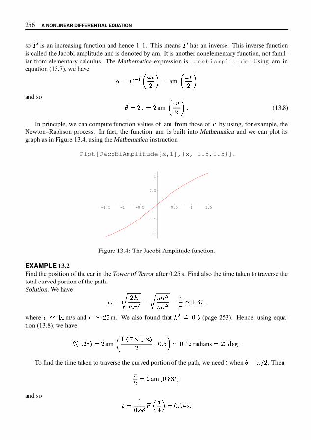
256 A NONLINEAR DIFFERENTIAL EQUATION
so�
is an increasing function and hence 1–1. This means�
has an inverse. This inverse functionis called the Jacobi amplitude and is denoted by am. It is another nonelementary function, not famil-iar from elementary calculus. The Mathematica expression is JacobiAmplitude. Using am inequation (13.7), we have
� � � � � � � � � � am � � � �and so
� � � � am � � � � � (13.8)
In principle, we can compute function values of am from those of�
by using, for example, theNewton–Raphson process. In fact, the function am is built into Mathematica and we can plot itsgraph as in Figure 13.4, using the Mathematica instruction
Plot[JacobiAmplitude[x,1],{x,-1.5,1.5}].
-1.5 -1 -0.5 0.5 1 1.5
-1
-0.5
0.5
1
Figure 13.4: The Jacobi Amplitude function.
EXAMPLE 13.2Find the position of the car in the Tower of Terror after 0.25 s. Find also the time taken to traverse thetotal curved portion of the path.Solution. We have
� � � �� � � � � � � �� � � � � � � � � � � �where � � � � m/s and � � ! m. We also found that " � �� $ � ! (page 253). Hence, using equa-tion (13.8), we have
� & $ � ! ( � am � � � � � + $ � ! - $ � ! � � $ � � radians � / � 1 �To find the time taken to traverse the curved portion of the path, we need � when
� � 3 4 . Then3 � am & $ � 5 5 � ( �and so � � �$ � 5 5 � 8 3 � 9 � $ � ; � s �

THE ENERGY EQUATION 257
�It is important to appreciate the similarity between the method of solution of this problem and the
way we solved the oscillation problem on page 215 and the air pressure problem on page 210. There isa systematic approach here which is applicable to more problems than just these three, and it is worthdevoting some effort to understanding it. In both cases the differential equation leads us to define afunction with a given derivative by means of an integral. The solution is then obtained by using theinverse of this function. The difference is in the definition of the new function. In this problem it is
� � � � �
�
� �� � � � � � � � � � �
whereas in the air pressure problem it was
� � � � �
�
�� � �
and in the oscillation problem it was
� � � � �
�
� �� � � � �
�
13.1.2 The case � " # $ &The cases � ' " # $ & and � " # $ & do not arise in the Tower of Terror, but they do arise inother situations—for example in the simple pendulum. There are also amusement park rides wherea train oscillates or rotates on the interior of a circular track. Before continuing, let’s make a fewremarks about the simple pendulum. In spite of the name, you will find that a full analysis of thesimple pendulum is anything but simple. In fact, the name is only there to distinguish it from thecompound pendulum which we shall not consider. A simple pendulum consists of a mass of negligibledimensions suspended from a fixed point by an inelastic rigid rod of negligible mass. We require arigid rod rather than a string, so that the pendulum is able to oscillate through any angle, or even rotatecompletely around its point of suspension. The motion of the pendulum depends on its velocity, andhence energy, at
*and it might oscillate, rotate or in the transitional case, simply move to the top of
the circle and remain there.To solve the differential equation of motion for the case � " # $ & , we use similar methods to
the previous case � , " # $ & , but the functions which arise are different. We will simply quote theresults and use Mathematica to plot the relevant functions.
In the case of low energy ( � ' " # $ & ), the system oscillates and the solution is given by� � / � " � � � 2 � � � sn � / � � (13.9)
where � � � 7 � " # $ & � , � � $ 7 & and sn is a function called the Jacobi elliptic sine function. Itsdefinition is in terms of the Jacobi amplitude am and is given by
sn � � > � � � � � � � am � � > � � � � �It is contained in Mathematica , where it is denoted by JacobiSN. Its values can be calculated andits graph plotted as for any other function.
For various values of � , we can use equation (13.9) to get graphs of the solution�
as a function oftime. The exact nature of the solution will depend on the initial conditions, namely that at the lowest

258 A NONLINEAR DIFFERENTIAL EQUATION
point, the body has velocity � . We expect that the amplitude of the oscillations will increase as �increases, and this is indeed what happens. Before plotting these graphs, it is interesting to look at acommon approximation that is normally made for the simple pendulum. The equation of motion is
� � � � � � � � � � � � � �which we write as � � � � � � � � � � � �If
�is small, then � � �
��
and the equation is approximated by� � � � � � � � � �
with initial conditions� � � � � � and
� � � � � � � � � . This is now a linear equation which we have seenbefore. Its solution is � � � � � �� �
� � � � � (13.10)
How good is the approximation (13.10)? We have drawn three graphs below for initial velocitiesof 8.3 m/s, 25 m/s and 30.5 m/s. In each graph, the solid line is the solution (13.9), while the dottedline is the approximate solution (13.10). The approximation is excellent for the first case, but getsworse as we increase the initial velocity.
-10 -5 5 10
-0.4
-0.2
0.2
0.4
Figure 13.5: The case � � " � # m/s, $ % � � � � ' , � � � � * # �Here, and in the next two graphs, we have used � � . / , � � 0 � " 1 and
� � 3 � � � � � * # � $ % � 5 � �� % �
-10 -5 5 10
-1.5
-1
-0.5
0.5
1
1.5
Figure 13.6: The case � � . / m/s, $ % � � � * 5 , � � � � * # �

CONCLUSION 259
-10 -5 5 10
-2
-1
1
2
Figure 13.7: The case � � � � m/s, � � � � , � � � � �
For completeness, we mention the case when � � � � � � . Here the body has just enough energyto reach the top of the circle, but not enough to go past it and rotate. In this case, � � � and so
�is
the function � � � ��
"#
$ %& � ( * , - � %
This function is an elementary function and can be calculated using suitable methods of integration.The elementary function solution we obtain is� � . � � * , - 0 1 � � � - � . 5where � � & � 8 � . The graph is plotted in Figure 13.8. Notice that
� � : and� � ( : are horizontal
asymptotes, indicating that the body takes forever to reach the top.
-8 -6 -4 -2 2 4 6 8
-4
-3
-2
-1
1
2
3
4
Figure 13.8: The critical case � � � � � �
13.2 CONCLUSIONThe functions we have used in dealing with this problem in circular motion may be unfamiliar, but theprinciples used for defining them by integrals and inverse functions are exactly the same as those fortrigonometric and inverse trigonometric functions that arose from the problem on the Anzac Bridge.As practical problems become more complicated, the functions which arise as solutions also becomemore complicated. This is simply a fact of life. Fortunately, much of the drudgery is now taken outof the calculations by tools such as Mathematica. Nobody has to do heroic calculations any more—computers are far quicker and more accurate—but we do need to understand the principles behindthese calculations.

This page intentionally left blank
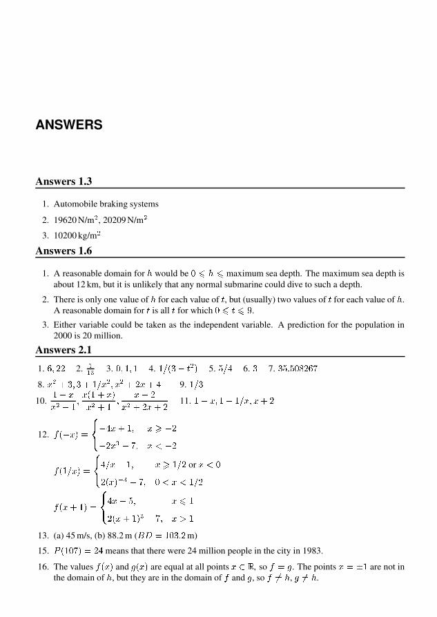
ANSWERS
Answers 1.3
1. Automobile braking systems
2. 19620 N/m � , 20209 N/m �3. 10200 kg/m �
Answers 1.6
1. A reasonable domain for � would be � � � � maximum sea depth. The maximum sea depth isabout 12 km, but it is unlikely that any normal submarine could dive to such a depth.
2. There is only one value of � for each value of � , but (usually) two values of � for each value of � .A reasonable domain for � is all � for which � � � � .
3. Either variable could be taken as the independent variable. A prediction for the population in2000 is 20 million.
Answers 2.1
1. � � � � 2. �� � 3. � � � � � 4. � � � � � � � ! 5. " � % 6. � 7. � " & " � ( � � *8. + � , � � � , � � + � � + � , � + , % 9. � � �
10.� � ++ � , � � + � � , + !+ � , � � + , �+ � , � + , � 11. � � + � � , � � + � + , �
12. < � � + ! ? @AB
� % + , � � + D � �� � + � � * � + I � �< � � � + ! ? @A
B% � + , � � + D � � � or + I �� � + ! K � � * � � I + I � � �
< � + , � ! ? @AB
% + , " � + � �� � + , � ! � � * � + N �13. (a) 45 m/s, (b) 88.2 m (
O Q ? � � � & � m)
15. T � � � * ! ? � % means that there were 24 million people in the city in 1983.
16. The values < � + ! and W � + ! are equal at all points + Y Z , so < ? W . The points + ? [ � are not inthe domain of � , but they are in the domain of < and W , so < \? � , W \? � .

262 ANSWERS
17. � � �� � � � � � � � � �18. � � � � ��
� � � ! $ �� � ! * �
19. (a) � � , . ! where � is the number of vehicles, . is the population and , is some constant.
(b) � 1 � , 4 ! where � 1 is the kinetic energy, 4 is the velocity and , is some constant.
(c) 5 � , 6 ! where 5 is the surface area, 6 is the radius and , is some constant.
(d)7 � � 8 96 ! where
7is the force and
�is the universal gravitational constant.
Answers 2.2
1. : ; = � ! @ � 2. : B C � E ; : B C � E 3. � � @ ! I J ; = � ! @ �4. : B C � � ! � E ; : 5. = � ! � � ; = � ! � � 6. = � ! @ � ; = O � ! @ �7. P � R � � R S � T U � 8. P � W � � W O � S T 9. Z \ * ^
10. � \ \ @ (or ` � � 11. � \ \ � 12. � \ * a or $ � �13. � * \ b 14. � @ \ \ @ (or d : � 15. d = � ! � �16. d � U @ � 17. d � � @ ! @ � 18. d = � � ! @ �19. d � � h ! � � 20. d � � @ ! � � J j = � ! @ � 21. No such exists.
Answers 2.3
2. Use the ranges � * * � , � * * � � , � * * � a k6. � � k T O 6 . This is easier to see if you take the scale on the axis as multiples of O 6 .
Answers 2.4
1. : ; = � � ! @ � 2. n� � ! � � ; :3. o $ � and o * � � ; = � ! @ � 4. : ; = � � ! @ �5. All n� � ; All p p $ � 6. : ; :7. P � � � � � ! P � � k Z � � � k b � h ! P � � � � � k � b ^ ! P � � � � � k � � Z8. As one example P � � � t � O � � ! � � * * �O � � ! � \ * �
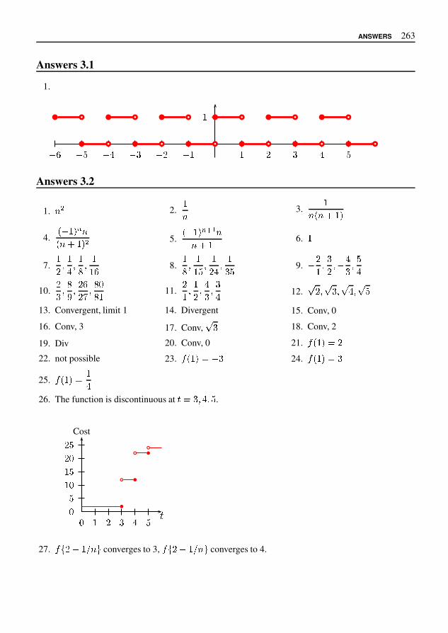
ANSWERS 263
Answers 3.1
1.
� � � � �� �� �� �� �� �� �
�
Answers 3.2
1. � 2.�
� 3.�
� � � � � �
4.� � � � � �
� � � � � 5.� � � � � � � �
� � � 6. �
7.�
� � �� � �
� � �� � 8.
�� � �
� � � �� � � �
� � 9. � �� � �
� � � �� � �
�10.
�� � �
" � � �� # � � %
� � 11.�
� � �� � �
� � �� 12. ' � � ' � � ' � � ' �
13. Convergent, limit 1 14. Divergent 15. Conv, 0
16. Conv, 3 17. Conv, ' � 18. Conv, 2
19. Div 20. Conv, 0 21. ) � � � + �22. not possible 23. ) � � � + � � 24. ) � � � + �
25. ) � � � + ��
26. The function is discontinuous at / + � � � � � .
% � � � � �%�
� %� �
� %� �
6
Cost
27. ) 8 � � � 9 � : converges to 3, ) 8 � � � 9 � : converges to 4.

264 ANSWERS
28. The graphs of � � � � � and � � � � � � � � are shown in the diagram.
�� � �
�
� �
�
�
29. The diagram shows � � � � � � � .
�� � �
31. � � � �
��
� �
32. � � � �
��
� �
33. ��
��
�� �
�
� �34. �!
Answers 4.1
1. " 2. � � 3. $ � % � 4. � $ � ' 5. � ( 6. � $ )
7. * + � � . � 8. * + � � . 9. * + � � . �10. * + � � . � $ � � � � � 11. 4 + � � . " 12. 6 + � � . � � � "
13. The function * + is differentiable at all points except . � . The graph of * + is shown in thediagram:
� � �
�
� �
<
14. Both are differentiable at . � (and at all other points).
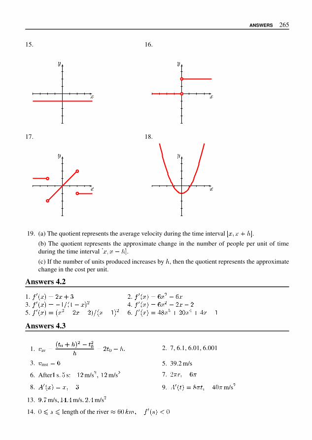
ANSWERS 265
15. 16.
�
�
�
�
17. 18.
�
�
�
�
19. (a) The quotient represents the average velocity during the time interval � � � � � � .(b) The quotient represents the approximate change in the number of people per unit of timeduring the time interval � � � � � � .(c) If the number of units produced increases by , then the quotient represents the approximatechange in the cost per unit.
Answers 4.2
1. � � � � � � � � � 2. � � � � � � � � � � �3. � � � � � " # � " � � � � 4. � � � � � � � � � � � �5. � � � � � � � � � � � � # � � " � � 6. � � � � � . 0 � 1 � � 2 � 3 � . � � "Answers 4.3
1. 4 av � � 5 7 � � � 5 �7 � � 5 7 � = 2. 7, 6.1, 6.01, 6.001
3. 4 inst � � 5. 39.2 m/s
6. After " s � ? s @ " � m/s � � " � m/s � 7. � B C � � B8.
E � � � � � � � � 9.E � � 5 � � 0 B 5 � . 2 B m/s �
13. H = J m/s � " . = . m/s � � = . m/s �14. 2 L M L length of the river � � 2 O P � � � M � R 2

266 ANSWERS
15. Approximately 0.08% per hour; approximately 0.025% per hour; before 12 min and after 3.6hours. Note that if a person was involved in a serious accident after 5 minutes and then breathal-ysed by the police half an hour later, that person would probably have a hard time convincing thepolice that he or she was under the legal limit at the time of the accident.
16.� � � � � � �
� � � � � The weight decreases as the ship moves away from the earth.
Answers 5.1
1. It is best to use central differences in this problem.
(a) � � � � � � � � � � � � , � � � � � � � � � � � � , � � � � � � � � � � � � , � � � � � � � � � � � � , � � � � � " � � � � �(b) The graph is the straight line of slope 0.6 and passing through the origin.
(c) � � � % � � � � � % �(d) � � % � � � � � % � + � � � - � � � � . � � � � � � �
2. Again, we use central differences.
(a) / � � � � � " � " , / � � � � � � � � � , / � � . � � � � �(b) The acceleration is decreasing, so / � � % � is negative.
(c) 66 m/s
Answers 5.2
1. 3 � � - 6 � � - � � � - ; � � 2. 3 � 6 � � � �3. 3 � � - 6 � � � � 4. 3 � � � � - 6 � �
6. > � % � � % �� + % + � 7. C � % � � % F
� + � % �� + � %
8. / � % � � % �� + % H + � % + �
9. The equation of motion is J � M % H � . The seventh observer has made an error. The readingshould be 1.99, not 1.91.
Answers 5.3
2. The ball takes longer to fall than to rise. [Use energy considerations.]
3. " � � � m 5. � � N �6. Differentiating your answer should give the differential equation you started with.
Answers 5.5
1. Increases on � � P - � � � and � � - P � , decreases on � � � - � �2. Increases on � � �
� - P � , decreases on � � P - � �� �
3. Increases on � � �� - P � , decreases on � � P - � �
� �

ANSWERS 267
4. Increases on � � �� � � , decreases on � � � � � �
�
5. Global minimum of � � at � � � , no local maximum
6. Local maximum of � at � � � , local minimum of � � � at � � � �7. Local maximum of � � at � � � , global minima of � at � � � �8. No local extreme values, no stationary points
9. Global minimum of � � at � � � , global maximum of � at � � � , local maximum of � � at � � �10. The rectangle should be a square of side � cm.
11. � � � " � � �12. Width of base: � � cm, height of sides: % ' % cm
Answers 6.1
1.( )
( + � � � ' � � )
Answers 6.2
1. � � 2. � % 3. � / 4. 015. � � 6. 23 4 25 4 22 2 7.
�� 8. 6
9.�% 10. 4 11.
�� / � 12. � �
%
13.
8�
� 9 2: 14.
8�� 9 2
� � : � � 15.3�
� 9 2
�� : 4 � 16.
?�� 9 2
�
17.8�
� 9 2
�: � : 4 � 18. �
A�� 9 2
� : 4 � � � � �19. 9 20. � �
21. � � �22. 3/5
23. Use the fact that � 4 � 4 � 4 I I I 4 K is an arithmetic progression.
24. L � � � � � �
: 4 � � L 8 � � � 25. L � � :
: 4 � � L 8 � �
26. L � � :� � : 4 � � L 8 � �
� 27. L � � � :� 4 � : � L 8 � �
Answers 6.3
1. � ' � � � � � S2. � � � � � T
3. � ' % / � � � S4. � � � � ' � � % � S
5. � ' � � � � � T
6. � � % ' % � � � T7. � ' � � � � � T
8. � ' � � � � � S9. % � T
10. � ' � / � � � S
12. 3.049. This is about 3% accuracy.
13. � � � � � ' � � ' � / � � � � error W � ' � � � � / �

268 ANSWERS
14. � � � � � � � � � � � � � � � � � error � � � � � � � � �Answers 6.4
1. � 2. � 3. � � � � 4. � 5. �6. � 7. � � 8. � 9. � 10. �
11. � ! # ! � 12. & ( ! # ! �13. & � ! # ! � 14. & � ! # ! �15. & � ! # ! �16. The terms in the sum on the right-hand side are smaller for a given value of / , so that we expect
the right-hand side to converge more quickly.
Answers 6.5
1. Radius of convergence 0 � � 3 4 � # 0 � 9 � # 9 � # < 9 � = # > 9 ? ? ?3. 3 4 0 C , C 4 0 & 34. From the previous question, 3 4 4 0 C 4 0 & 3 so 3 4 4 9 3 0 � . Similarly C 4 4 9 C 0 � .
5. The series converges for & � ! # ! � , by the ratio test, so it is differentiable for & � ! # ! � .We then have 3 4 � # 0 � & # < 9 # O & # � 9 ? ? ? , which is a geometric series with sum � � � � 9 # < .
Answers 6.6
1. � 3 C � # 0 � � 9 # < � � C 3 � # 0 � 9 # <2. � 3 C � # 0 �� # 9 � & � � � C 3 � # 0 W # & �# & �3. � 3 C � # 0 # 9 � # � � C 3 � # 0 Y # < 9 #4. � 3 C � # 0 � # 9 � < � � C 3 � # 0 # < 9 �5. � 3 C � Z 0 � Z < & (Z < & � � � C 3 � Z 0 � Z \ � 9 � Z ]6. � 3 C � # 0 � � � � � C 3 � # 0 �7. � # � � 9 # < 8. � � # < � � 9 # > >9. � � � Z < 9 � Z � Z > 9 � Z < 9 � > 10. = � � & � � ` < � ` 9 � � ` a
Answers 6.7
1. & � c � > e 2. & � # c � e � 3. f< � c & c � 4. � � � � & c > e > 5.
� c e� c e 9 � < 6. � # < c < e 9 � # > c < e7. � � � # < 9 # 9 � c e � g < g f 8.
# c e� � 9 # < 9. � � � � �10. � � � = �

ANSWERS 269
11. � � � � � �� � � � � � � � �� � 12. Here is one of many possibilities: � � � � � � � � � ! # � # &� � � & # � # !Answers 6.81. * + & & & 2. , & - + 3. � , . � mg 4. / � , 1 2 4 7. * , 7 � , � C 8. � * 7 - * kg
Answers 7.2
2. � � : � & 7 The displacement after 2 s is & 7 & � < > ? � : � & m.
Answers 7.3
5. � ? A B � < > ? � 6. � < > ? � E < > ? * E � * ? A B � E ? A B * E7. � � < > ? � � � � ? A B � 8. � 1 � � < > ? K � 1 � � ? A B K9. � �� � < > ? � 10. + ? A B � < > ? � � � � ? A B � � � �
11. � ? A B � � : * < > ? �12. � O � � � � < > ? � � � R� & S � O � & � does not exist.
13. � � � � � < > ? � � V � � � � ? A B �Answers 7.6
6. � � ? � < � � � 7. ? � < � � ? A B � � � � � B � < > ? � �8. � cosec , � < > � , � 9. cosec � � � � � � cosec � � < > � � �
10. Y ? A B � [� [ \ ] � as � [ ] &Answers 8.1
1. L 2. NL ( / / O term) 3. L
4. L 5. NL ( / � term) 6. L
7. NL ( � � O O � � , � O � , � � terms)
8. L
9. / � ` 1 a � 4 � b 1 a 4 10. / � ` 1 a c 4 � b11. / � � ` � b � � 1 a 4 12. / � � ` � b � � 1 a � 413. / � ` 1 a 2 4 � b 1 414. / � ` 1 a
� e f� e 2 4 � � � b 1 a
� e a� e 2 4 � �
15. / � � � � 1 a 2 4 16. / � � 1 4 � 1 � 417. / � � ` � b � � 1 h 4 18. / � ` 1 a h 4 � b 1 4

270 ANSWERS
19. � � � � � � � � � 20. � � � � � � � � � �21. � � � � � � � � � � � 22. � � � � � � � � � � � �23. � � � � � � � � � � � 24. � � � � � � � � � � � �25. � � � � � � � � � � � � � 26. � � � � � � � � � � �27. � � � � � � � � � � � 28. � � � � � � � � � � � �29. � � � � � �
� ��
30. � � � � � � � � � � � �
31. � � � � � � � � � � � � � � � � � � � � � � � � � 32. � � �� � � � � � �
33. � � � � � � � � � � � � � � � � � � � � � � � � � 34. � � � � � � � � � � � � � � �35. � � � � �
� � � �
36. � � � � � � � � � �
37. � � � � � ��
� � � �38. � � � � � �
� � � �� � �
39. � � � �� � � � �
� � � 40. � � � � � � � � � � � �Answers 8.2
1. 2 2. � ! 3. 2 4. " #5. $ 6. � # 7. " & ! 8. " # " & (9. # " $ 10. # " $ 11. � " & ( � ! , � 12. � # � & #
13. 0 � 3 14. ( 15. � & 6 16. � & 8 & (17. �� : �� : 18. �� �� : 19. � �� : � �� : 20. � �
� � � ;� �
21. " & ( 8 # 22. , cis& & ?
@ 23. $ cis?
! 24. , " $ cis?
,
25. $ " $ cis! ?
, 26. ! cis! ?
$ 27. " $ cis# ?
, 28.&
$ � � & A " & # �
29.&
! � � & A " $ � 30. � & C &$ A " !
$ 31. & C � &$ A " !
$32. A & C A
33. A &$ A " !
$Answers 8.3
1. � � � � �Answers 8.4
1. � � � � � � � � G I J $ J M N $ �
2. � � � � � � ��
� G I J " ! $ J M N " !
$�
3. � � � G I J � J M N � 4. � � � � � � � G I J ! J M N ! �
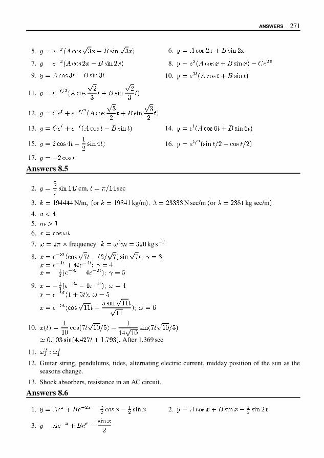
ANSWERS 271
5. � � � � � � � � � � � � � � � � � � � � 6. � � � � � � � � � � � � �7. � � � � � � � � � � � � � � � � � � 8. � � � � � � � � � � � � � � � � " � # �9. � � � � � % � � � � � � % 10. � � � # � � � � % � � � � � % �
11. � � � � �
� ) � � � � �� % � � � � � � �
� % �
12. � � " � � � � � �� # � � � � �
� % � � � � � � �� % �
13. � � " � � � � � � � � � % � � � � � % � 14. � � � � � � � + % � � � � � + % �15. � � � � � 0 % 3 4
� � � � 0 % � 16. � � � �� # � � � � % 7 � 3 � � % 7 � �
17. � � 3 � � � %Answers 8.5
2. � � :; � � � 4 0 % cm, % � ? 7 4 0 sec
3. @ � 4 B 0 0 0 0 N/m C � or @ � 4 B D 0 4 kg/m� C � � � � � � � N sec/m � or � � � � D 4 kg sec/m � G4. H J 05. L M 46. � � � � � %7. � � � ? S frequency T @ � � # L � � � V kg s
� #8. � � � � ) � � � � � ; % � � � 7 � ; � � � � � ; % T � �
� � � � X � � 0 % � � X � T � 0� � 3 \) � � � ] � 3 0 � � # � � T � :
9. � � 3 \) � � � ] � 3 0 � � X � � T � � 0� � � � ` � � 4 � : % � T � � :� � � � ` � � � � � 4 4 % � : � � � � 4 4 %
� 4 4 � T � � +
10. � � % � � 44 V � � � ; % � 4 V 7 : � 3 4
4 0 � 4 V � � � � ; % � 4 V 7 : �� V G 4 V � � � � � 0 G 0 � ; % � 4 G ; B � � G After 1.369 sec
11. � ## � � #\12. Guitar string, pendulums, tides, alternating electric current, midday position of the sun as the
seasons change.
13. Shock absorbers, resistance in an AC circuit.
Answers 8.6
1. � � � � � � � � # � 3 )# � � � � \# � � � � 2. � � � � � � � � � � � 3 \) � � � � �3. � � � � � � � � � 3 � � � �
�

272 ANSWERS
4. � � � � � � � �� � � � � � � � � � � � � � � � � � �
5. � � � � � � � � � � � � � � � � � � �! " � � � � # ! �! " � � � � 6. � � � � � & � � � � � & � !� & � � � &7. � � � � � � � � � � � # � � � � 8. � � �
� � � � � � � & # �� � & � � � � &
9. � � �� � # � 2 � � � & # � � � � & 610. 2 & 6 � � � � � 9 � � ! "� 11. 2 & 6 � � � � � & � � � � � & � � �12. 2 & 6 � � � � � � � � � 9 �
13. 2 & 6 � � � 9 � � � � � &14. 2 & 6 � � 9 � � � � � � # !� 15. 2 & 6 � � � � � � � � � # � & � � �16. (a) = � � , (b) 2 & 6 � � � A � � � � � � � C so 2 & 6 D � as & D H . The transient part of the
solution is 2 & 6 � � � A � � � � �and the steady state part is 2 & 6 � � .
17. The initial value problem describing the motion is � I K K 2 & 6 � " � I � � I � � � � & , 2 I 6 � I , K 2 I 6 � I . The solution to this is
2 & 6 � # W� ! � � � � � & � WX � � � � � & Z18. Regular pushing on a swing. Unwanted feedback in public address systems. Tuning a radio: by
tuning a dial, the natural frequency in the receiving circuit is made equal to the frequency of thebroadcast waves of the sending station. The circuit resonates with the transmitted signals andabsorbs peak energy from the signal.
19. (a)� 2 & 6 � � # � � � \ � � � � � & � W � � � � � & ] ^ � 2 & 6 � � � � � � � � � &
(b)� 2 & 6 � !! I W 2 ! � � � � # ` � 9 � # � � � � � & � � � � � & 6 ^ � 2 & 6 � � � 9 � 2 � # ! 6
20. ! I I I �Answers 9.3
1. A b W � � � � � 2. A � b W # f� � � � � � �3. � � � # f9 � � � � � � 4. # !� �5. A b W # 9 b � � � 6. 2 # � 6 9 b � � �7. & 9 � & � �

ANSWERS 273
Answers 9.5
2. Yes
Answers 9.6
1. 155 2. 686 3. 506
4. 152 5. 259 6. 518
7. 44000 8.�
�� � � � � � � � � 9.
��
� � � � � � � � � �
10. �
� ��
� ��
11. 28 12. 125
13. 124 14. 155 15. 9
16. 42
Answers 9.7
1. � ! # % ' � ( � * ! # % ' � � � � 2. � ! # - ' . ( % � � * ! # - ' . ( 0 �
3. � ! # - ' � % � % � * ! # - ' � % ( . 4. � ! # � ' � � % � � * ! # � ' � � % 0 (
5. � ! # � ' . � � ( � * ! # � ' . � % � 6. � ! # � ( ( � * ! # � � � ' � �
7. The area of the cross-section is 11.1 m ; the volume of water per second is 5.51 m � /sec.
8. 2.6498 (6 subintervals)
9. 19 intervals
10. 20 intervals
Answers 9.8
1. � � 9 2. � � : < = � 9 3. 9 � ? 9
4. @ � B ��
5. � 9 � � 9 � � � 6. . C : < = . C �
7. � 9 � � 9 � 9 � � 8. � 9 � � 9 � �
Answers 9.9
1.�
� 9 � .2.
� 99 � �
3..
� � 94.
�9 I = 9
5. � 9 I = � 9 � � � �� 9 �
9 � �6.
� � � 9 9 � � � 9 �
7.�
� 9 8.
� 9� 9 �
9.� 9
� � 9 ��
� 9 � � 9 �
10.� � � 9 � � 9 �
� � � � 9 � � 9 � �
11.� B R S
9 � B R S12. (a) � � ' ( . (In fact 2.512) (b) A straight line

274 ANSWERS
13. (b) � � � � � � � 14. (c) About 20 000 kilograms
15. (a) 10 Watts/m � , (b) 130 Db
Answers 10.1
1. � � � � � � � �� 2. The function is not 1–1.
3. The function is 1–1 and so has an inverse. It is difficult to find a formula for the inverse. Newton’srule can be used to compute function values.
4. The function is not 1–1. This can be proved by showing that � � � � � � # has two solutions for$ # $ ' � .
5. � � � � � * �� � � , � �6. � � � � � � � � �� � �
7. is not 1–1 8. � � � � � � � �/9. � � � � � � � � � � � � 10. � � � � � � � � � �
11. � � � � � �� � �Answers 10.2
1. � 2. � 3. � �4. � � � 5. 3 4 � � � 6. � � ��7. � 4 � 6 7 8 � � � � 8. � � � � 4 � : 7 = 6 7 8 � � = A B �� � 9. � : 7 = � � 4 � 6 7 8 : 7 = � � � � B � �
10.� � 4 6 7 8 �� E �
11.� 6 7 8 � � � 4� E � � 6 7 8 6 7 8 � � �6 7 8 � �
12. 1.41421 13. 1.25992 14. 0.739085
15. 1.86081 16. 0.876726 17. 3.44949
18. 1.47502 19. 1.25992 20. 0.346574
21. 20.0855 22. 0.523599 23. 2.44949
25.� 6 7 8 �6 7 8 � � � � G hrs
26. Take H � � � I/ � � � J day� . The population doubles after 25 years and triples after 39.6 years.
27. 3.817 days, 8.86 days 28. 37 000 years
29. About 14 minutes 30. 10.08 pm

ANSWERS 275
Answers 10.5
1. � � � 2. � � � 3. � � � 4. � � �5. � � � 6. � � � 7. � � � 8. � � 9. � � � 10. � � � 11. 0 12. � �
13.� � � � 14.
� � � 15. � 16. � � � �17. � 18.
� � �� 19. � 20. � 21. �22. � � � � � � � � �
� � � � � � � � 23. � � � � � � � � � � 24. � � � � � � $ % & ( * , - . � � � � � 025.
1 21 � � ( * , � � , 6 7 � � 26.1 21 � � � �� � � � � 8 � �
27.1 21 � � � � � : � � � 28. � � � ; � � ;< ; < � ; �
29.� � � % � � ? * @ � � � � B %
Answers 11.1
1. 2 � D � � E ( * , � � D � G , 6 7 � � D 2. 2 � D � � E ( * , � � D � G , 6 7 � � D3. 2 � D � � $ - 8 � � E ( * , � � D � G , 6 7 � � D �4. � � D � � $ � � E ( * , � � D � G , 6 7 � � D �
Answers 11.2
13. � � � � � � � , 6 7 � � � � � � 14. � � � � � � � � � ( * , � � 815. � � � � � � csch � � 16. � � � � � � � ( * � � � �17. � � � � � � � ( * , � � � , 6 7 � � 18. � � � � � � � � 7 � � �19. � � � � � � � � � , 6 7 � � 8 20. � � � � � � � , 6 7 � � ? * @ � �21. � � � � � � � � � 7 � � 22. � � � � � � � � � ( * , � �23. � � � � � � ( * , � ( * , � � , 6 7 � � 24. � � � � � � � ( * , � �25. � � � � � � S ( * � � S � 26. � � � � � � sech � T � � U

276 ANSWERS
27. (b) The limiting velocity is � � � � � . This is the terminal velocity of the body. No matter howfar it falls, it never exceeds this velocity.
(c) � � � � � � � � � � � � � � � � �� � � � � �
Answers 11.3
1. � � � � � !" # � $ % ' 2. � � � � � ! �� ' � ' � � $ � $3. � � � � � % ' ' % � $ � � � 0 � 1 2 � 4. � � � � � '" � $ � ' � '" � $ % '5. � � � � � 4 � 5 0 � �� 4 $ � � � � $ � � ' 6. � � � � � 8 � 5 0 � 1 2 � � $" ' � � $7. � � � � � ' ' % � $ � � � 0 � 1 2 � 8. � � � � � sech �9. � � � � � �: � : " � $ % ' 10. � � � � � �: � : " � $ � '
Answers 12.2
1. 1 2. " ! % = � # 3. 93 4. = � #5. = � ! 6. � 5 0 � # 7. 0 8. " 8 % '9. 21/64 10. 2 11. 4 12. 2
Answers 12.3Note: The constant of integration has been omitted in the answers below.
1. � $ � ' � $! 2. % � � � @ �# 3. B C �
4. � � $ � ' 5.!8 � � ' � D � $ 6.
!E � D � # � D � $7.
� 5 0 � D8 8. % ! � � � " � 9.! " 4 � J � LJ M
10.'8 4 � $ � ! J � � � � D � $ 11.
� � � � � $! 12. % B � � � �13.
'! � � � ' � � 5 0 � ! � � 14. � � � : � 5 0 � Q :15. % Q " ' % Q $! � � 5 0 1 2 Q! 16.
8 ! � � � � � $17.
'! � � � � � � � $ � 18. � � 0 1 2 � � $!
19. % � � 0 � 1 2 � ' % B $ � 20. � 5 0 1 2 � 5 0 � �

ANSWERS 277
Answers 12.4Note: The constant of integration has been omitted in the answers below.
1. � � � � � � 2. � � � � � � � �3. � � � � � � � � � � � � � � 4. � � � � � � � ! � � �5. � � � � � � � � !� % � ' � ! � � � � 6.
� �+ � � � � � � !, � � � � � � ! � � �7. � � �0 � � � � � � � � � � � 8. � � 5, � � 5+ % � ' �9. � 7 8 � �� � !� � � � �
� � 9 7 8 � �� : 10. % � ' � � � � � � � � � �11. � � � � � ! � � � � � � � � � � � � � � � � � �12. � !� � % � ' ��13. � � � % � ' � � � � � � � % � ' B cosec � � � � � B � � �14.
� � 5� D � � � 5, % � ' � � � 5+ � % � ' � � �Answers 12.5Note: The constant of integration has been omitted in the answers below.
1. % � ' 9 ! � �� � � : 2.!� % � ' 9 ! � �� � ! :
3. % � ' 9 � � �� � � ! : 4.!0 % � ' 9 � � +� � � :
5.% � ' �� � � % � ' � ! � � � � 0� % � ' � � � � � 6.
!� � � � � � � � !8 % � ' 9 � � !� � ! :7. % � ' � � !� % � ' � ! � � � � 8. � � � � � � � % � ' 9 ! � �7 ! � � � :9.
7 �+ � � � � � �7 � � !I % � ' 9 � � !� � ! : 10.D+ % � ' 9 � � 0� � � :
11. � !� % � ' � ! � � � � � % � ' � � � � � � + � % � ' � + � � �12. � !7 + � � � � � 9 ! � � �7 + : � % � ' � � !� % � ' � � � � � � ! �13. � J
8 � � � � � � � 14. % � ' 9 ! � � �� � � � :15. I K � 5 � + % � ' 9 K � 5 � !K � 5 � ! : � K 16. 0 % � ' 9 L � M! � L � M :

278 ANSWERS
Answers 12.7Note: The constant of integration has been omitted in the answers below.
1.�� � � � � � � � �� �
2. � �� � � � � � � � � � �� � � �� � � � � � � � � 3.
�! � � � � � � � � �! � � � � � � & 4.
�� � � � � � � � � � ' (� � �5.
�� � � � � � � ) + � � � �� �6.
�� ! � & � � � � � � � � �� � � � � � � 3 � � 4 � 5 �7. � � � � � � � � �� � � � � � � � � 5 8. � �� � � � � � � � � � �� � � � � � � � � � � � � 9. � �� � � � � � � � � � �� � � � � � �
10. � � � � � � � � � � �

This page intentionally left blank

This page intentionally left blank

Index
Bold face page numbers are used to indicatepages with the primary information about theentry, such as a definition or an explanation.
abuse of notation, 58acceleration, 55alternating series, 114amplitude
of a complex number, 138of SHM, 146
antiderivatives, 169Anzac Bridge, 7, 9, 109Archimedes, 176area under a curve, 171Argand, 136Argand diagram, 135argument
of a complex number, 138Aristotle, 4asymptotes, 23atmospheric pressure, 6auxiliary equation, 129
complex roots, 133distinct roots, 130repeated roots, 132
backward differences, 61barometer, 5beats, 159
Cardano, 134central differences, 61, 76chain rule, 96complementary
equation, 153function, 153
complexconjugate, 138exponential, 141
plane, 135series, 140
complex number, 134amplitude, 138argument, 138Cartesian form, 138imaginary part, 135modulus, 138phase, 138polar form, 138real part, 135
composition of functions, 96concave down, 72concave up, 72concavity, 73conjugate pairs, 139continuity, 28
at a point, 33on a closed interval, 37on an open interval, 37
continuous, 28continuous function, 33, 37convergent sequence, 32convergent series, 82cosecant, 125cosine function, 113cotangent, 125critical damping, 149
damping, 145de Moivre’s theorem, 143decreasing function, 68, 69derivative, 45
of � � � � , 188of � � � , 116of � � , 116of � � � � , 125of �
� , 52, 204of a constant function, 49

282 INDEX
of a product, 50of a quotient, 52of a square root, 204of a sum, 49of an inverse function, 204of inverse trigonometric functions, 219
differencesbackward, 61central, 61, 76forward, 61
differentiable, 41, 44differential equation, 61
homogeneous linear, 129linear, 129nonlinear, 129second order, 111solved using Mathematica, 67
differentiating a power series, 93differentiation
by first principles, 45logarithmic, 193
discontinuous, 28domain, 12domain, natural, 12, 13Dreamworld, 3
elementary function, 225elementary functions, 252elliptic functions, 254energy, 215error term, 114Euler, 141Euler’s formula, 141exponential function, 87
general, 212extreme value, 70
finite differences, 46flight 811, 4fluid pressure, 5forced oscillations, 156forward differences, 61frictional forces, 128function, 8, 12
continuous, 32, 33, 37decreasing, 69differentiable, 28, 44graph of, 17
increasing, 69primitive, 169rational, 25, 57smooth, 27, 28value, 12
Galileo, 58, 66general exponential function, 212general solution, 103, 130geometric series, 82graph
of a function, 17plotting with Mathematica, 17
hectopascal, 75homogeneous, 129hyperbolic functions, 225, 227
increasing function, 68, 69indefinite integral, 170independent variable, 12infinite series, 81initial value problem, 63input number, 11, 12integral, 170
indefinite, 170integration by parts, 241integration by substitution, 239intersection, 15interval
closed, 15infinite, 15open, 15
intervals, 15inverse function, 197, 200, 201inverse function values, calculating, 205inverse hyperbolic functions, 230inverse sine, 218inverse trigonometric functions, 218
Jacobi amplitude, 256
kinetic energy, 215
left-hand sum, 177Leibniz, 45linear
combination, 130

INDEX 283
differential equation, 128local maximum, 70local minimum, 70logarithmic differentiation, 193
maximumabsolute, 71global, 71local, 70
method of undetermined coefficients, 155millibars, 75minimum
absolute, 71global, 71local, 70
modulusof a complex number, 138
natural domain of a function, 13natural domain of a rule, 12Newton, 45Newton’s method, 206Newton–Raphson method, 206nonlinear, 252numerical properties, 8
Olympic Games, 1one–to–one, 200output number, 11, 12
partial fractions, 243partial sums, 82particular integral, 153particular solution, 103, 153parts, integration by, 241pascal, 75pendulum,simple, 251periodic, 122periodic functions, 116periodicity, 116phase
of a complex number, 138phase angle, 146physical laws, 66point of inflexion, 71, 73
horizontal, 71polar form
of a complex number, 138
polynomial, 21potential energy, 215primitive, 170primitive function, 169principle of superposition, 130products of functions, 50projectile motion, 58pump, 7
quadratic integrals, 247quotients of functions, 50
radius of convergence, 90range, 12Raphson, 206rate of change, 54ratio test, 85, 141rational function, 25rational functions, 57, 244recurrence relation, 112resonance, 158restriction, 12Riemann sum, 176right-hand sum, 177
secant, 125second derivative, 45sequence, 32
convergent, 32divergent, 32
simple harmonic motion, 145, 146simple pendulum, 251Simpson, 206Simpson’s rule, 183sine function, 113solution
general, 103, 130of a differential equation, 61particular, 103trial, 62
square wave, 30stationary point, 71steady state, 161stretched string, 127strong damping, 148substitution, integration by, 239sum
Riemann, 176
284 INDEX
sums of functions, 49superposition, principle of, 130
Tacoma Narrows Bridge, 7tangent, 125Torricelli, 5Tower of Terror, 1, 57transient, 160trapezoidal rule, 182trial solution, 62, 104trigonometric functions as ratios, 119trigonometric identities, 116turning point, 71
undetermined coefficients, 154union, 15
variable, 9variation of parameters, 104velocity, 53
weak damping, 147

![Standing on the Shoulders of Giants - zenspider.com · Standing on the Shoulders of Giants MWRC 2015, SLC, UT Ryan Davis, Seattle.rb @the_zenspiderx "we [the Moderns] are like dwarves](https://static.fdocuments.net/doc/165x107/5ecdc6be23e7e560b14fb3fc/standing-on-the-shoulders-of-giants-standing-on-the-shoulders-of-giants-mwrc-2015.jpg)