On the Setup of a Test Bench for Predicting Laminar-to ... · On the Setup of a Test Bench for...
14
Journal of Energy and Power Engineering 10 (2016) 411-424 doi: 10.17265/1934-8975/2016.07.005 On the Setup of a Test Bench for Predicting Laminar-to-Turbulent Transition on a Flat Plate Pascal Bader and Wolfgang Sanz Institute for Thermal Turbomachinery and Machine Dynamics, Graz University of Technology, Inffeldgasse 25/A, Graz 8010, Austria Received: May 5, 2016 /Accepted: May 19, 2016 /Published: July 31, 2016. Abstract: At turbomachinery relevant flow conditions the boundary layers are often transitional with laminar-to-turbulent transition occurring. The characteristics of the main flow can depend highly on the state of the boundary layer. Therefore it can be vitally important for the designer to understand the process of laminar-to-turbulent transition and to determine the position and length of the transitional region. In this paper the flow over a flat plate is experimentally studied in order to investigate and better understand transitional flow. Preston tube measurements as well as a thermographic camera system were performed for two different inlet velocities in order to determine the position of the transitional zone. The results of the experiment are compared to numerical flow solutions using a common transition model to determine its capability. The simulation has been performed with the two commercial codes CFX ® and Fluent ® by Ansys ® and an in-house code called LINARS. As a result of this study, a better understanding of the experimental and numerical methods for determining transition shall be given. Key words: Boundary layer transition, computational fluid dynamics, Preston tube, thermographic camera, flat plate boundary layers. Nomenclature Decay exponent Wall friction coefficient crit Critical value Frequency ܪHydraulic/Characteristic diameter ܪChannel height Turbulence kinetic energy ܭAcceleration parameter ܮPhysical integral length scale ܮPlate length Pseudo-integral scale Mixing length mean Mean value ݑNusselt number Local static pressure ௧ Total pressure ݍ ݍ/∞ Non-dimensional dynamic pressure Reynolds number ݑTurbulence intensity ݑLocal streamwise velocity ݑ∞ Free-stream velocity Corresponding author: Pascal Bader, Dipl.-Ing., BSc, research assistant, research field: measurement and simulation of boundary layer behavior. W Channel width ݔStreamwise coordinate ݕDistance to the wall ݕା Dimensionless wall distance ߙHeat transfer coefficient ߜBoundary layer thickness ߜ כDisplacement thickness Dissipation rate ߥKinematic viscosity ௐ Wall shear stress ௧ Turbulent shear stress ∞ Free-stream value ഥ Mean value Fluctuation Abbreviation ACF Autocorrelation function BL Boundary layer CFD Computational fluid dynamics FFT Fast fourier transformation FRAPP Fast-response aerodynamic pressure probe ITTM Institute for Thermal Turbomachinery and Machine Dynamics LDV Laser Doppler velocimetry LE Leading edge PIV Particle image velocimetry D DAVID PUBLISHING
Transcript of On the Setup of a Test Bench for Predicting Laminar-to ... · On the Setup of a Test Bench for...
Journal of Energy and Power Engineering 10 (2016) 411-424 doi: 10.17265/1934-8975/2016.07.005
On the Setup of a Test Bench for Predicting
Laminar-to-Turbulent Transition on a Flat Plate
Pascal Bader and Wolfgang Sanz
Institute for Thermal Turbomachinery and Machine Dynamics, Graz University of Technology, Inffeldgasse 25/A, Graz 8010, Austria
Received: May 5, 2016 /Accepted: May 19, 2016 /Published: July 31, 2016. Abstract: At turbomachinery relevant flow conditions the boundary layers are often transitional with laminar-to-turbulent transition occurring. The characteristics of the main flow can depend highly on the state of the boundary layer. Therefore it can be vitally important for the designer to understand the process of laminar-to-turbulent transition and to determine the position and length of the transitional region. In this paper the flow over a flat plate is experimentally studied in order to investigate and better understand transitional flow. Preston tube measurements as well as a thermographic camera system were performed for two different inlet velocities in order to determine the position of the transitional zone. The results of the experiment are compared to numerical flow solutions using a common transition model to determine its capability. The simulation has been performed with the two commercial codes CFX® and Fluent® by Ansys® and an in-house code called LINARS. As a result of this study, a better understanding of the experimental and numerical methods for determining transition shall be given. Key words: Boundary layer transition, computational fluid dynamics, Preston tube, thermographic camera, flat plate boundary layers.
Nomenclature
Decay exponent
Wall friction coefficient
crit Critical value
Frequency
Hydraulic/Characteristic diameter
Channel height
Turbulence kinetic energy
Acceleration parameter
Physical integral length scale
Plate length
Pseudo-integral scale
Mixing length
mean Mean value
Nusselt number
Local static pressure
Total pressure / ∞ Non-dimensional dynamic pressure
Reynolds number
Turbulence intensity
Local streamwise velocity
∞ Free-stream velocity
Corresponding author: Pascal Bader, Dipl.-Ing., BSc,
research assistant, research field: measurement and simulation of boundary layer behavior.
W Channel width
Streamwise coordinate
Distance to the wall
Dimensionless wall distance
Heat transfer coefficient
Boundary layer thickness
Displacement thickness
Dissipation rate
Kinematic viscosity
Wall shear stress
Turbulent shear stress
∞ Free-stream value
Mean value
Fluctuation
Abbreviation
ACF Autocorrelation function
BL Boundary layer
CFD Computational fluid dynamics
FFT Fast fourier transformation
FRAPP Fast-response aerodynamic pressure probe
ITTM Institute for Thermal Turbomachinery and Machine Dynamics
LDV Laser Doppler velocimetry
LE Leading edge
PIV Particle image velocimetry
D DAVID PUBLISHING

On the Setup of a Test Bench for Predicting Laminar-to-Turbulent Transition on a Flat Plate
412
SST Shear stress transport
TE Trailing edge
1. Introduction
The boundary layer represents the small zone
between the wall and the free stream where viscous
effects are important. Due to its size, the influence of
its state (laminar or turbulent) is often neglected
although it can have a high impact on the flow
characteristics like heat transfer or wall friction. These
parameters influence the efficiency as well as the
thermal stress of, for example a turbine blade.
Many parameters like free-stream velocity,
acceleration, free-stream turbulence etc. have an
influence, if a boundary layer is laminar or turbulent,
but at the first contact of a flow with a stationary
structure the boundary layer starts laminar and will
become turbulent (under the right flow conditions) via
a transitional area. The boundary layer passes through
several stages within this transitional zone until it
becomes fully turbulent [1].
It is vitally important to understand the influence of
the above stated parameters on the onset and length of
the transitional zone in order to influence and
potentially control the state of the boundary layer.
Because of the possibility to increase efficiency,
transition also plays a major role in turbomachinery
flows. In such machines the efficiency of blades and
stages can be improved when considering transition;
thus this gives the possibility to improve the overall
engine performance. In 1991, Mayle [2] published an
interesting overview of the role of transition in gas
turbines. He analyzed experiments performed by
different research groups and showed the influence of
several flow parameters on the transition process.
Additional experiments were performed in the last
years by different research groups. Yip et al. [3]
performed inflight measurements and predicted
transition with the help of Preston tubes and analyzed
the influence of the flight condition on the boundary
layer around an airfoil. Oyewola et al. [4, 5] showed
how the flow in the boundary layer can be measured
with the help of hot-wire probes as well as LDV
(laser-Doppler velocimetry). Another optical
measurement technique has been used by Widmann et
al. [6] who performed near-wall measurements with a
PIV (particle image velocimetry) system. Also hot-film
measurements were performed by Mukund et al. [7].
In addition to measurements, also different
numerical approaches have been developed to predict
the laminar-turbulent transition process. Common
models, for example the [8] and the
Θ [9, 10] model. For the latter model, various
correlations for important model parameters have been
developed [11-15].
So far, only the transition from laminar to turbulent
has been described, but under certain flow conditions
(like high acceleration) a reverse-transition or
relaminarization from turbulent to laminar can occur.
Up to now only few measurements and publications
have been made in order to understand relaminarization.
Therefore, a project has been launched at the ITTM
(Institute for Thermal Turbomachinery and Machine
Dynamics) at Graz University of Technology in order
to understand the different mechanisms leading to
relaminarization.
The first step of this project is to set up a test bench
in order to measure transition from laminar to turbulent.
This should help to improve the understanding of
transition even further and to test different
measurement techniques. Another point of this
measurement campaign is to acquire all data necessary
for the simulation since the vital parameter of the
turbulence scale is not documented in most
experimental works. Some works discuss the
measurement of turbulence length scales, for example
Camp and Shin [16] who described in detail how to
process the measured signal in order to get the
necessary values. Also Axelsson et al. [17, 18], and
Craft [19] discussed different length scales and
measurements of turbulence intensity.
This work focuses on the set up of the test bench and
will give an overview of technical considerations

On the Setup of a Test Bench for Predicting Laminar-to-Turbulent Transition on a Flat Plate
413
which should be taken into account. Additionally
measurement techniques are discussed and a special
focus lies on measuring of the turbulence length scale.
Finally, several CFD codes and transition models
will be compared in order to see their differences and
their capabilities in predicting transition within the test
bench.
2. Numerical Setup
The computational mesh models the flow region in
the test bench which is described in the next section
(Fig. 1b) and consists of about 13 million cells. To
ensure a mesh independence of the simulation result,
the -value of the mesh was kept between 0.1 and
1 as recommended in Ref. [20]. The mesh consists
only of the upper part of the channel and is illustrated in
Fig. 1a.
The computational simulations have been performed
with three different codes: ANSYS® CFX® v15.0,
ANSYS® Fluent® v15.0.0 and the in-house code
LINARS.
CFX® solves the Navier-Stokes equation system
with first-order accuracy in areas where the gradients
change sharply to prevent overshoots and undershoots
to maintain robustness, and with second-order in flow
regions with low variable gradients to enhance
accuracy [20].
Fluent® uses the simple algorithm for the
pressure-based solver. The pressure correction
equation is solved with second-order accuracy and the
momentum as well as the turbulence and transition
equations are solved with a third-order MUSCL
algorithm.
LINARS has been developed at Graz University of
Technology at the ITTM [21]. The code solves the
RANS (Reynolds-averaged Navier-Stokes) equations
in conservative form with a fully-implicit,
time-marching finite-volume method. The inviscid
(Euler) fluxes are discretized with the upwind flux
difference splitting method in Ref. [22]. The
incompressible solutions are obtained with a
pseudo-compressibility method.
For the simulation with all three codes Menter’s
SST turbulence model [23] was used with the
Θ [12] transition model. Additionally, with
Fluent® the [8] turbulence/transition
model was also applied.
3. Experimental Setup
The measurements are performed in a subsonic
wind tunnel located at the ITTM. The test rig is a
continuously operating open-loop wind tunnel. The air
is delivered by a 125 kW radial compressor with a flow
rate of approximately 0.6 kg/s. The compressor delivers
the air into a flow settling chamber. From this chamber
the air is transported via a flow-calming section
(a) Computational mesh
(b) Subsonic turbine with measurement area
Fig. 1 Illustration of the test bench and computational mesh.

On the Setup of a Test Bench for Predicting Laminar-to-Turbulent Transition on a Flat Plate
414
formed by a diffuser with guiding vanes towards the
test area. A schematic drawing of the test bench is
given in Fig. 1b.
Transition measurements have been performed for
two different inlet velocities: ∞, = 5.3 m/s (low
speed case) and ∞, = 13.2 m/s (high speed case).
The plate in the channel is inclined by 2° as
recommended by Coupland [24]. This should ensure
that the flow is attached to the plate without leading
edge separation bubbles.
In order to minimize the influence of the channel
walls on the measured boundary layer some aspects
have been kept in mind and will be discussed in the
following.
First, the position (normal to streamwise direction)
of the plate leading edge (distance a in Fig. 1b) has
been chosen. One aspect here is that the plate must not
be inside the boundary layer of the bottom or top wall
of the channel. Therefore the approximate size of the
boundary layer was estimated. The size of the
boundary layer depends amongst others on the
development length. It can be approximated with the
Blasius solution for the laminar boundary layer:
(1)
and for the turbulent boundary layer:
0.382 / (2)
where, is the local boundary layer thickness, is
the development length and is the Reynolds
number based on [1]. For the calculation of the
Reynolds number and are taken at the inlet.
These two equations are illustrated in Fig. 2a which
gives an example of the boundary layer growth for a
specific velocity (here about 5 m/s). In this illustration
of the boundary layer thickness , 3 10 is
assumed for the onset of transition. According to
Schlichting and Gersten [1], this is valid for “normal”
longitudinal flow along a flat plate with a sharp
leading edge. Additionally they state that, this
critical Reynolds-number can be increased to
, 10 by ensuring a smooth flow (low
turbulence intensity).
Although it is not clear, if these transition onset
criteria stated by Schlichtung and Gersten are valid for
the designed test bench, it is a good start for estimating
the beginning of transition. In the following,
, 3 10 is assumed as the onsetlocation of
the transitional zone within the test bench of the
institute.
The 1 value of the bottom and top wall,
respectively, can be estimated with about 3.3
10 for the low-speed case and 8 10 for
the high-speed case which results in a boundary layer
thickness of about 30 mm and 25 mm,
respectively, at the end of the plate. The plate leading
edge is placed at about 100 mm above the bottom
wall so that it certainly does not lie inside a wall
boundary layer. But due to the small channel height,
the influence of the sidewall and top wall BLs has to be
considered in the numerical analysis. Another aspect
which should be kept in mind is the vertical position of
the TE (trailing edge) of the plate (distance b in Fig.
1b). It has to be ensured that the boundary layer of the
top wall does not “collide” with the investigated
boundary layer of the plate. As already described the
boundarylayer grows along the plate, thus an important
value is the boundary layer thickness at the
trailing edge of the plate. In Fig. 2b this value is
illustrated for different free stream velocities ∞. Also
the values for the two test cases are marked in the
figure. The graph shows that there is a maximal BL
thickness (about 30 mm) which can be
reached for a given plate length under normal operating
conditions.
The position of the trailing edge could not be chosen
freely, since the length of the plate is fixed with 939
mm and the angle is set to 2° as discussed before.
However, so the resulting position of the TE has
sufficient distance towards the top wall.
1 Computed with the plate length L and the thermophysical properties at the inlet.

On the Setup of a Test Bench for Predicting Laminar-to-Turbulent Transition on a Flat Plate
415
(a) Along the plate
(b) At the plate trailing edge where v changes in Re
Fig. 2 Graph of the boundary layer thickness .
Also the displacement thickness is important
which describes the shift of the free-stream streamlines
away from the surface where the boundary layer
develops. It gives the distance which a surface with a
boundary layer would have to be moved in
perpendicular direction to have the same flow rate
compared to a case of a surface without a boundary
layer [1]. The displacement thickness can be calculated
for an incompressible fluid with
1∞
∞
(3)
where, represents the local streamwise velocity,
the direction normal to the wall and ∞ represents the
free stream velocity. influences the velocity of the
free-stream within a channel (like in the test setup)
since it narrows down the effective free stream flow
area.
The tests were performed for two different channel
cross sections W × H: 500 × 200 mm (low speed case)
and 200 × 200 mm (high speed case).
4. Turbulence and Dissipation Measurements
Downstream of the diffuser with guiding vanes
(position A in Fig. 1b) the free stream turbulence
intensity together with the total pressure is
measured. These values are measured about x = 220
mm upstream of the leading edge of the plate and are
used as boundary conditions for the simulation.
Close to the leading edge (position B) again the
turbulence intensity is measured to be able to
approximate the turbulence length scale of the flow
which is necessary for the computational setup.
measurements were performed by means of a
cylindrical single-sensor FRAPP (fast-response
aerodynamic pressure probe). A miniaturized
On the Setup of a Test Bench for Predicting Laminar-to-Turbulent Transition on a Flat Plate
416
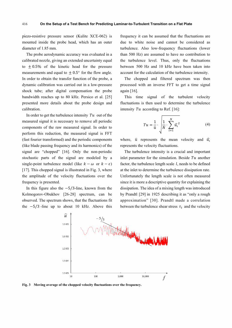
piezo-resistive pressure sensor (Kulite XCE-062) is
mounted inside the probe head, which has an outer
diameter of 1.85 mm.
The probe aerodynamic accuracy was evaluated in a
calibrated nozzle, giving an extended uncertainty equal
to 0.5% of the kinetic head for the pressure
measurements and equal to 0.5° for the flow angle.
In order to obtain the transfer function of the probe, a
dynamic calibration was carried out in a low-pressure
shock tube; after digital compensation the probe
bandwidth reaches up to 80 kHz. Persico et al. [25]
presented more details about the probe design and
calibration.
In order to get the turbulence intensity out of the
measured signal it is necessary to remove all periodic
components of the raw measured signal. In order to
perform this reduction, the measured signal is FFT
(fast fourier transformed) and the periodic components
(like blade passing frequency and its harmonics) of the
signal are “chopped” [16]. Only the non-periodic
stochastic parts of the signal are modeled by a
single-point turbulence model (like or )
[17]. This chopped signal is illustrated in Fig. 3, where
the amplitude of the velocity fluctuations over the
frequency is presented.
In this figure also the 5/3-line, known from the
Kolmogorov-Obukhov [26-28] spectrum, can be
observed. The spectrum shows, that the fluctuations fit
the 5/3 -line up to about 10 kHz. Above this
frequency it can be assumed that the fluctuations are
due to white noise and cannot be considered as
turbulence. Also low-frequency fluctuations (lower
than 500 Hz) are assumed to have no contribution to
the turbulence level. Thus, only the fluctuations
between 500 Hz and 10 kHz have been taken into
account for the calculation of the turbulence intensity.
The chopped and filtered spectrum was then
processed with an inverse FFT to get a time signal
again [16].
This time signal of the turbulent velocity
fluctuations is then used to determine the turbulence
intensity according to Ref. [16]:
1 1 (4)
where, represents the mean velocity and
represents the velocity fluctuations.
The turbulence intensity is a crucial and important
inlet parameter for the simulation. Beside another
factor, the turbulence length scale , needs to be defined
at the inlet to determine the turbulence dissipation rate.
Unfortunately the length scale is not often measured
since it is more a descriptive quantity for explaining the
dissipation. The idea of a mixing length was introduced
by Prandtl [29] in 1925 describing it as “only a rough
approximation” [30]. Prandtl made a correlation
between the turbulence shear stress and the velocity
Fig. 3 Moving average of the chopped velocity fluctuations over the frequency.
On the Setup of a Test Bench for Predicting Laminar-to-Turbulent Transition on a Flat Plate
417
gradient in a viscous layer. Therefore he introduced the
mixing length which describes the mean free
distance between two eddies [1].
Although it is only a model for understanding the
process of dissipation, it is still used in modern CFD
codes. Since it is only a theoretical quantity, it is
neglected in most measurements, and in most
publications no focus on the length scale or dissipation
is laid on.
In the following different definitions of the
turbulence length scale are given. Several overviews
have been published in the last years like Refs. [16, 17,
31, 32] and in the following the main outcomes will be
discussed.
To use the above discussed mixing length in CFD
calculations, a correlation between the mixing length
and the dissipation rate is necessary. This
correlation is known as Prandtl-Kolmogorov-equation
[1].
//
(5)
where, represents the turbulence kinetic energy and
/ represents an empirical constant (usually 0.09)
which is specified by the used turbulence model [33].
This correlation is used by codes like Fluent®,
LINARS and several other codes. For estimating this
mixing length the Fluent® modeling guide recommends
lm with
0.07 (6)
where, represents the hydraulic/characteristic
diameter.
Other CFD codes (like CFX®) use a length scale
defined as /
(7)
This definition of a length scale is often called
pseudo-integral scale as suggested by Gamard and
George [31].
The two given definitions above (Eqs. (5) and (7))
represent a relation between the turbulence kinetic
energy and dissipation, but the problem is that and
are not directly measurable.
Since the length scale is used to define the turbulent
dissipation rate it is obvious to measure this flow
variable directly. Unfortunately this is almost
impossible, since it would be necessary to measure
down to very small spatial resolutions which cannot be
resolved by probes [17].
A length which is measurable is the so-called
(physical) integral length scale which is defined as
Ref. [16].
(8)
where, represents the ACF (autocorrelation
function) of the turbulent velocity signal. In order to
determine the chopped FFT spectrum which was
used within the signal processing for obtaining the
turbulence intensity is multiplied by its conjugated
complex part and then transformed back with an
inverse-FFT. The time signal obtained this way is then
autocorrelated [16].
The idea behind the integral length scale is that it
describes the time a turbulence fluctuation needs to
dissipate its energy. This time then is converted with
the mean velocity to a physical length.
The problem evolving from these definitions is that
the idea of a turbulence length as parameter for the
dissipation is more or less rough and dissatisfactory. So
far, three different length scales have been defined:
(1) The physical integral scale which is
measurable;
(2) The pseudo-integral scale which is used e.g. by
CFX®;
Table 1 Measured and computed values of and at the inlet (Pos. A) and within the channel (Pos. B).
Turbulence
Position A: 9.24%
Position B: 9.0%
Dissipation
Linear develop: 14.686 m2/s3
Exponent develop: 15.2485 m2/s3

On the Setup of a Test Bench for Predicting Laminar-to-Turbulent Transition on a Flat Plate
418
(3) The mixing-length idea which is used e.g. by
Fluent®;
While and have a clear relationship (
/ ), the relation between or and is not clear
and depends on the investigated flow.
In order to get a boundary condition for the
dissipation rate another approach will be discussed
within this work.
As discussed before, the fluctuations are measured at
two positions: At the inlet of the test section and within
the channel (positions A and B in Fig. 1b). At these
positions the turbulence intensity is determined. The
-values are given in Table 1.
Using the measured turbulence values at the two
different positions the dissipation rate can be
determined directly. Starting from the transport
equation for with the assumption of a
non-accelerating flow with a isotropic turbulence the
equation for the change of the turbulence kinetic
energy [32]
(9)
can be used. For a steady flow without turbulence
production between the two measurement positions
following approximation can be used:
(10)
Since the used evaluation system gives the
turbulent kinetic energy is obtained by using Eq. (11)
32
%100
(11)
at both measurement positions. Since the distance
between these two measurement positions is known as
well as the kinetic energy at these positions, can
be estimated by using Eq. (10). In a first approach a
linear decrease of the turbulence kinetic energy
between the two positions is assumed, thus is
constant.
Another approach is to assume an exponential
decrease of between the two measurement positions
according to
(12)
where, can be seen as decay exponent and describes
how the turbulence dissipates within the flow. Eq. (12)
can be used to calculate at any position based on a
starting value .
Since , and the distance are known in our
test case, the decay exponent for the wind tunnel can
be computed and thus the gradient of at the inlet
/ . Inserting this into Eq. (10) leads to the
dissipation rate at the inlet which can be calculated
with
(13)
The results of these evaluations are given in Table 1
where represents the solution with a linear and
with an exponential decrease of , respectively. Due to
the small change of the measured turbulence intensity
the difference between the two -values is small.
To sum up, five different options for the
determination of the turbulence dissipation have been
showed: Three length scales (physical integral length
scale , pseudo-integral scale and mixing length )
and two -values.
In Table 2 the different length scales are listed:
represents the measured value, represents the
mixing-length used by LINARS and Fluent® ( is the
mixing-length as recommend by the Fluent modeling
guide (see Eq. (6))) and represents the
pseudo-integral length scale used by CFX®. The
suffixes and represent the dissipation assumption
whether it is linear or exponential.
Table 2 clearly shows that the differences between
the different length scales are remarkable. To see the
influence of the different length scales, simulation
results computed with Fluent® and CFX® are given in
Fig. 4. The graph shows the development of the
turbulence intensity from the inlet to the
measurement position B.
The measured physical integral length scale L =

On the Setup of a Test Bench for Predicting Laminar-to-Turbulent Transition on a Flat Plate
419
Table 2 Different length scale in meters.
Measurement 0.18158
Fluent, modeling guide value 0.014
Fluent, from measured , 0.0575 Fluent, from measured , 0.0554 CFX, from measured 0.35 CFX, from measured 0.337
0.18158 m shows a too weak dissipation, while the
recommended mixing length = 0.014 m shows a
too high dissipation. Both length scales do not fit with
the measured decrease of turbulence intensity.
The pseudo-integral scales and mixing lengths
computed from the measured -values show nearly the
same decrease of turbulence intensity as the measured
one. It is also observable, that the differences between
the assumed linear and exponential turbulence decrease
are not high, but the exponential decrease fits slightly
better to the measured results.
Both CFX® simulations show a too high turbulence
intensity at the inlet, although the same value of =
9.24% has been specified. However, CFX® computes
the same decrease of compared to Fluent® and the
measurement.
For the sake of completeness it has to be mentioned
that LINARS (also using the mixing-length approach)
computes the same development as Fluent®, but is not
illustrated in Fig. 4 due to clarity of the chart.
5. Transition Measurements
In this section the measurement and visualization of
the transition process at the flat plate are discussed.
Along the flat plate several static pressure tappings
are embedded into the plate. The diameter of the
tappings is 0.5 mm. These measurement positions are
used for Preston-tube measurements.
A Preston tube is traversed all over the plate in
streamwise direction in order to locate the transition
region. The probe consists of a pitot tube with an inner
diameter of 0.5 mm. The Preston tube allows to
measure the dynamic pressure close to the wall. This
pressure can then be used to calculate the non-dimensional
dynamic pressure according to Ref. [35]:
Fig. 4 Simulation results with different length scales.
∞
,
,∞ (14)
where, , and represent the total and
static pressure acquired by the probe and the tappings,
and ,∞ represents the free-stream total pressure. The
result gives an indication of the shape of the velocity
profile close to the wall which is then characteristic for
the state of the boundary layer. Fig. 5 explains this
idea: The upper sketch shows the different velocity
profiles of the laminar and turbulent boundary layer.
The higher velocity close to the wall of the turbulent
boundary layer is due to the fact that more energy can
be transported normal to the streamwise direction
towards the wall because of its turbulent state [34].
The lower sketch in Fig. 5 shows the streamwise
distribution of the non-dimensional dynamic pressure
/ ∞ (here / ) and gives an example how the
value increases when transition occurs.
However, the probe size has to be kept in mind, since
the measured result can only be valid as long as the
thickness of the boundary layer is at least twice the
distance of the probe from the wall ( in Fig. 5).
As already described, two measurements were
performed for two different inlet velocities: ∞, =
5.3 m/s and ∞, = 13.2 m/s. The turbulence
intensity together with the total pressure have been

On the Setup of a Test Bench for Predicting Laminar-to-Turbulent Transition on a Flat Plate
420
Fig. 5 Explanation of the Preston tube measurement theory.
measured at the inlet plane and the turbulence
additionally close to the leading edge of the plate. The
values at the inlet plane together with the static
pressure at the outlet are used as boundary conditions
for the simulations described later.
In Fig. 6 the static pressure along the flat plate is
illustrated. The laminar and the turbulent zone are
separated by a small peak within the static pressure
which is caused by laminar-to-turbulent transition.
The measured / ∞ values of both test runs
are given in Fig. 7. No transition can be observed for
the low speed test case. This also agrees with the above
mentioned critical Reynolds number , as onset
criterion. According to this, transition would start at
about the position of the trailing edge of the plate.
The high speed measurements clearly show the start
of transition (rise of / ∞) at about 350-400 mm.
This again agrees with the assumed onset criterion
stated above.
In order to verify the measured transition location,
the change of the boundary layer is visualized with the
help of a thermographic camera. Since the heat transfer
coefficient depends highly on the state of the boundary
layer, the surface temperature of a heated plate changes
when the boundary layer transitions from laminar to
turbulent. The difference in heat transfer can be
described by the heat transfer coefficient which can
be calculated with the Nusselt-number defined as
(15)
where, represents the thermal conductivity.
changes with the state of the boundary layer according
to Ref. [36]:
0.332 . . laminar (16)
0.0296 . / turbulent (17)
where, represents the Prandtl number. The
correlation between and and thus
isillustrated in Fig. 8 ( = 0.71486 for air at 20 °C, 1
bar). In this graph again the critical Reynolds number
Fig. 6 Static pressure along the flat plate for the high speed test case.

On the Setup of a Test Bench for Predicting Laminar-to-Turbulent Transition on a Flat Plate
421
Fig. 7 / ∞ measurements along the flat plate.
of 3 10 is assumed as transition onset criterion.
For the visualization a FLIR® SC620 thermographic
camera was used which has a sensitivity < 40 mK at
30 °C. The camera was placed above an optical access
at the top of the channel (illustrated in Fig. 1b) and
recorded about 100 mm of the plate length.
On the flat plate a heating foil was glued with a
constant heating input. The optical access was placed
in such a way, that it is situated above the expected
transition zone.
The result of the visualization is given in Fig. 9. The
picture shows that the temperature of the heating foil
drops at about 410 mm plate length. This most likely
indicates a transitional zone and agrees well with the
results of the Preston probe measurements.
6. Transition Simulation
Both measurement techniques showed that transition
occurs at approximately 400 mm plate length. In the
following numerical results are compared with the
measurements to see how the transition model can
predict the measured transition zone.
All inlet conditions are taken from the measurement.
For the length scale , 0.0575 for Fluent® and
LINARS and 0.35 for CFX® are used which
have been computed from the measured dissipation
rate .
Fig. 10a shows the skin friction coefficient at the
plate for all three simulations. is defined as
12 ∞
(18)
where, is the wall shear stress and ∞ is the free
stream velocity. All three codes used the
Θ -model and Fluent® additionally the
-model. All three codes failed in predicting the
measured transition zone with the Θ model.
The skin friction values show a fully turbulent
boundary layer along the plate surface.
On the other hand, the turbulence
model predicted successfully a transitional zone
although it starts more upstream compared to the
measured transition location.
A possible reason for not predicting transition with
the Θ-model is observable in Fig. 10b which
shows the skin friction development along the flat plate
for different turbulence intensities computed with
Fluent®. The chart shows, that for decreasing inlet
Fig. 8 Nusselt number over Reynolds number for laminar and turbulent boundary layer.

On the Setup of a Test Bench for Predicting Laminar-to-Turbulent Transition on a Flat Plate
422
Fig. 9 Recording of the thermographic camera.
(a) Comparing the three codes
(b) Comparing different levels with Fluent®
Fig. 10 Computed development of skin friction coefficient
along the flat plate.
turbulence intensity transition is predicted. With
an inlet turbulence intensity of about 2.2% the
simulation shows a similar transition position as the
measurements. At 1% no transition is
observable anymore since the boundary layer stays
laminar along the whole plate. It seems that for the high
inlet turbulence the Θ transition model is not
able to predict a laminar flow at the leading edge of the
plate; thus no transition can be observed.
In Fig. 10b, also the model result is
given for a lower inlet turbulence intensity. For
3.5% this model predicts a similar onset of the
transition zone as the measurements. Compared to the
Θ -model result, the transitional zone is also
smaller, which agrees better with the measurements,
since the increase of / ∞ spans only the distance
between two measurement positions (see Fig. 7).
Both models show a different behavior when
varying the turbulence intensity, but both react sensibly
to the boundary condition.
7. Summary and Conclusions
In the present work the transition on a flat plate has
been investigated. The measurements and simulations
performed in the scope of this work are intended for a
better understanding of transition prediction, both
experimentally and numerically.
First, the paper describes the setup of a test bench.
Therefore several important considerations are
described which should be followed when designing
such a test facility.
One major outcome of the study is that the
turbulence inlet boundary conditions of the numerical
simulations have a high impact on the result of the
simulation, especially when it comes to transition. The
investigation also showed that there are differences in
the definition of the turbulence length scales and the
needed length scale for the simulation cannot be
measured directly. A general correlation between the
measured integral length scale and the pseudo-length
scale used by CFD would be helpful, but this needs
more experimental data.
Two different techniques to measure and visualize
transition have been tested successfully: Preston tube
measurements and visualization with a thermographic
camera. Regarding the computational results, the
Θ-model was not able to predict the transition
process of this test case as observed in the measurements.
On the other hand the turbulence model
could predict transition but at a more upstream position.

On the Setup of a Test Bench for Predicting Laminar-to-Turbulent Transition on a Flat Plate
423
Further numerical studies are necessary to understand
the deficiencies of these models.
Further experimental and numerical studies are
planned and should help to better understand the
complex mechanism of transition. The result will form
the basis for further studies on the mechanism of
relaminarization.
Acknowledgement
The authors would like to especially thank Marn
Andreas, Selic Thorsten and Bauinger Sabine for their
immense support during the setup of the test bench and
the measurement campaign.
The authors would also like to thank the Austrian
Federal Ministry for Transport, Innovation and
Technology who funded the project RELAM within
the Austrian Aeronautics Program TAKE OFF.
References
[1] Schlichting, H., and Gersten, K. 2006. Grenzschicht-Theorie (Boundary-Layer Theory). Springer-Verlag Berlin Heidelberg.
[2] Mayle, R. E. 1991. “The Role of Laminar-Turbulent
Transition in Gas Turbine Engines.” Journal of
Turbomachinery 113 (October): 509-37.
[3] Yip, L. P., Vijgen, P., Hardin, J. D., and Van Dam, C. P.
1993. “In-flight Pressure Distributions and Skin-Friction
Measurements on a Subsonic Transport High-Lift Wing
Section.” Presented at AGARD, High-Lift System
Aerodynamics.
[4] Oyewola, O., Djenidi, L., and Antonia, R. A. 2003.
“Combined Influence of the Reynolds Number and
Localised Wall Suction on a Turbulent Boundary Layer.”
Experiments in Fluids 35 (July): 199-206.
[5] Oyewola, O. 2006. “LDV Measurements in a Pertubed
Turbulent Boundary Layer.” Journal of Applied Science 6
(14): 2952-5.
[6] Widmann, A., Duchmann, A., Kurz, A., Grundmann, S.,
and Tropea, C. 2012. “Measuring Tollmien-Schlichting
Waves Using Phase-Averaged Particle Image
Velocimetry.” Experiments in Fluids 53 (3): 707-15.
[7] Mukund, R., Narasimha, R., Viswanath, P. R., and
Crouch, J. D. 2012. “Multiple Laminar-Turbulent
Transition Cycles Around a Swept Leading Edge.”
Experiments in Fluids 53 (6): 1915-27.
[8] Walters, K., and Cokljat, D. 2008. “A Three-Equation Eddy-Viscosity Model for Reynolds-Averaged
Navier-Stokes Simulations of Transitional Flows.” Journal of Fluids Engineering 130 (12): (121401) 1-14.
[9] Menter, F. R., Langtry, R. B., Likki, S. R., Suzen, Y. B., Huang, P. G., and Völker, S. 2006. “A Correlation Based Transition Model Using Local Variables Part 1: Model Formulation.” Journal of Turbomachinery 128 (3): 413-22.
[10] Langtry, R. B. 2006. “A Correlation-Based Transition Model Using Local Variables for Unstructured Parallelized CFD Codes.” Ph.D. thesis, University Stuttgart.
[11] Elsner, W., Piotrowski, W., and Drobniak, S. 2008. “Transition Prediction on Turbine Blade Profile with Intermittency Transport Equation.” Journal of Turbomachinery 132 (1): 11-20.
[12] Langtry, R. B., and Menter, F. R. 2009. “Correlation Based Transition Modeling for Unstructured Parallelized Computational Fluid Dynamics Codes.” American Institute of Aeronautics and Astronautics Journal 47 (12): 2894-906.
[13] Sorensen, N. N. 2009. “CFD Modeling of Laminar-Turbulent Transition for Airfoil and Rotors
Using the – Θ Model.” Wind Energy 12 (8): 715-33.
[14] Malan, P., Suluksna, K., and Juntasaro, E. 2009.
“Calibrating the – Θ Transition Model for
Commercial CFD.” In Proceedings of the 47th AIAA Aerospace Sciences Meeting Including the New Horizons Forum and Aerospace Exposition, 1-20.
[15] Kelterer, M. E., Pecnik, R., and Sanz, W. 2010. “Computation of Laminar-Turbulent Transition in
Turbomachinery Using the Correlation Based – Θ
Transition Model.” In Proceedings of the ASME Turbo Expo, 613-22.
[16] Camp, T. R., and Shin, H. W. 1995. “Turbulence Intensity and Length Scale Measurements in Multistage Compressors.” Journal of Turbomachinery 117 (January): 38-46.
[17] Axelsson, L.-U., and George, W. 2008. “Spectral Analysis of the Flow in an Intermediate Turbine Duct.” In Proceedings of the ASME Turbo Expo, 1419-26.
[18] Axelsson, L.-U. 2009. “Experimental Investigation of the Flow Field in an Aggressive Intermediate Turbine Duct.” Ph.D. thesis, Chalmers University of Technology.
[19] Craft, T. J. 2011. Turbulence Length Scales and Spectra. Lecture Notes for Advanced Turbulence modeling, The University of Manchester.
[20] ANSYS. 2012. Ansys CFX-Solver Modeling Guide. Release 14.5. ANSYS Inc.
[21] Pecnik, R., Pieringer, P., and Sanz, W. 2005. “Numerical Investigation of the Secondary Flow of a Transonic Turbine Stage Using Various Turbulence Closures.” In Proceedings of the ASME Turbo Expo, 1185-93.

On the Setup of a Test Bench for Predicting Laminar-to-Turbulent Transition on a Flat Plate
424
[22] Roe, P. L. 1997. “Approximate Riemann Solver, Parameter Vectors, and Differencing Scheme.” Journal of Computational Physics 135 (2): 250-8.
[23] Menter, F. R. 1994. “Two-Equation Eddy-Viscosity Turbulence Models for Engineering Applications.” American Institute of Aeronautics and Astronautics Journal 32 (8): 1598-605.
[24] Coupland, J. 1990. “Flat Plate Transitional Boundary Layers.” ERCOFTAC “Classic Collection” Database. Accessed March 15, 2016. http://cfd.mace.manchester.ac. uk/cgi-bin/cfddb/ezdb.cgi?ercdb+search+retrieve+&&&SemiCFlow1g=Yes%%%%dm=Line.
[25] Persico, G., Gaetani, P., and Guardone, A. 2005. “Design and Analysis of New Concept Fast-Response Pressure Probes.” Measurement Science and Technology 16 (9): 1741-50.
[26] Kolmogorov, A. N. 1991. “The Local Structure of Turbulence in Incompressible Viscous Fluid for Very Large Reynolds Numbers.” Proceedings: Mathematical and Physical Sciences 434 (1890): 9-13.
[27] Kolmogorov, A. N. 1991. “Dissipation of Energy in a Locally Isotropic Turbulence.” Proceedings: Mathematical and Physical Sciences 434 (1890): 15-17.
[28] Obukhov, A. M. 1941. “On the Distribution of Energy in the Spectrum of Turbulent Flow.” Doklady Akademii
Nauk SSSR 32 (1): 22-4. [29] Prandtl, L. 1925. “Bericht Über Untersuchungen
Ausgebildeter Turbulenz.” Zeitschrift Für Angewandte Mathematik und Mechanik 5 (2): 136-9.
[30] Bradshaw, P. 1974. “Possible Origin of Prandtl’s Mixing-Length Theory.” Nature 249 (6): 135-6.
[31] Gamard, S., and George, W. K. 2000. “Reynolds Number Dependence of Energy Spectra in the Overlap Region of Isotropic Turbulence.” Flow, Turbulence and Combustion 63 (1-4): 443-77.
[32] Pope, S. B. 2000. Turbulent Flows. Cambridge: Cambridge University Press.
[33] ANSYS. 2015. “Using Flow Boundary Conditions.” In Ansys Fluent Documentation, Release 16.0. ANSYS Inc.
[34] Schlichting, H. 1965. Grenzschicht-Theorie (Boundary-Layer-Theory). Verlag G. Braun, Karlsruhe.
[35] Händel, D., Rockstroh, U., and Niehuis, R. 2014. “Experimental Investigation of Transition and Separation Phenomena on an Inlet Guide Vane with Symmetric Profile at Different Stagger Angles and Reynolds Numbers.” In Proceedings of the 15th International Symposiumon Transport Phenomena and Dynamics of Rotating Machinery, 1-9.
[36] Polifke, W., and Kopitz, J. 2005. “Wärmeübertragung.” Heat Transfer, Pearson Education, München.