SANDIA REPORT SAND2010-1480 Unlimited Release February 2010

On the Response of Rubbers at High Strain Rates Johnathan Greenberg Niemczura Prepared by Sandia National Laboratories Albuquerque, New Mexico 87185 and Livermore, California 94550 Sandia is a multiprogram laboratory operated by Sandia Corporation, a Lockheed Martin Company, for the United States Department of Energy’s National Nuclear Security Administration under Contract DE-AC04-94AL85000. Approved for public release; further dissemination unlimited.

2

Issued by Sandia National Laboratories, operated for the United States Department of Energy by Sandia Corporation. NOTICE: This report was prepared as an account of work sponsored by an agency of the United States Government. Neither the United States Government, nor any agency thereof, nor any of their employees, nor any of their contractors, subcontractors, or their employees, make any warranty, express or implied, or assume any legal liability or responsibility for the accuracy, completeness, or usefulness of any information, apparatus, product, or process disclosed, or represent that its use would not infringe privately owned rights. Reference herein to any specific commercial product, process, or service by trade name, trademark, manufacturer, or otherwise, does not necessarily constitute or imply its endorsement, recommendation, or favoring by the United States Government, any agency thereof, or any of their contractors or subcontractors. The views and opinions expressed herein do not necessarily state or reflect those of the United States Government, any agency thereof, or any of their contractors. Printed in the United States of America. This report has been reproduced directly from the best available copy. Available to DOE and DOE contractors from U.S. Department of Energy Office of Scientific and Technical Information P.O. Box 62 Oak Ridge, TN 37831 Telephone: (865) 576-8401 Facsimile: (865) 576-5728 E-Mail: reports@adonis.osti.gov Online ordering: http://www.osti.gov/bridge Available to the public from U.S. Department of Commerce National Technical Information Service 5285 Port Royal Rd. Springfield, VA 22161 Telephone: (800) 553-6847 Facsimile: (703) 605-6900 E-Mail: orders@ntis.fedworld.gov Online order: http://www.ntis.gov/help/ordermethods.asp?loc=7-4-0#online

3

SAND2010-1480 Unlimited Release

February 2010

On the Response of Rubbers at High Strain Rates

Johnathan Greenberg Niemczura University of Texas-Austin Campus Executive Fellow

Sandia National Laboratories

Computational Structural Mechanics and Applications P.O. Box 5800

Albuquerque, New Mexico 87185-0372

Abstract

In this report, we examine the propagation of tensile waves of finite deformation in rubbers through experiments and analysis. Attention is focused on the propagation of one-dimensional dispersive and shock waves in strips of latex and nitrile rubber. Tensile wave propagation experiments were conducted at high strain-rates by holding one end fixed and displacing the other end at a constant velocity. A high-speed video camera was used to monitor the motion and to determine the evolution of strain and particle velocity in the rubber strips. Analysis of the response through the theory of finite waves and quantitative matching between the experimental observations and analytical predictions was used to determine an appropriate instantaneous elastic response for the rubbers. This analysis also yields the tensile shock adiabat for rubber. Dispersive waves as well as shock waves are also observed in free-retraction experiments; these are used to quantify hysteretic effects in rubber.

4

ACKNOWLEDGMENTS I would like to thank Sandia National Laboratories for supporting me through the Sandia National Laboratory Campus Executive Fellowship.

5

CONTENTS

1. INTRODUCTION ............................................................................................................... 15

2. RUBBER ELASTICITY ..................................................................................................... 19 2.1 Rubber Structure ......................................................................................................... 19 2.2. Quasi-Static Tensile Testing ....................................................................................... 22 2.4. Relaxation ................................................................................................................... 32

3. THEORY OF ONE-DIMENSIONAL WAVE PROPAGATION....................................... 36 3.1 Equations of Motion ................................................................................................... 36 3.2 General Solutions for a Semi-infinite Strip ................................................................ 37

3.2.1 Fan Solution .................................................................................................... 37 3.2.2 Constant Solution............................................................................................ 38

3.3 Solution by Method of Characteristics ....................................................................... 38 3.4 Approximate Material Model for Rubber ................................................................... 40 3.5 Shock Jump Conditions and Driving Force ................................................................ 45 3.6 Shocks in a Cubic Material ......................................................................................... 46 3.7. Kinetic Relation .......................................................................................................... 48 3.8. Analysis of Free-Retraction Experiment in Rubber.................................................... 49

3.8.1. Governing Equations and General Solutions.................................................. 49 3.8.2. Unloading Waves in Cubic Material Model ................................................... 51

4. DISPERSIVE WAVES........................................................................................................ 52 4.1. Experimental Scheme for Generation of Impact-Induced Tensile Waves in Rubber. 53 4.2. Comparison of Measured and Calculated Particle Trajectories.................................. 56 4.3. Power-Law Model ...................................................................................................... 58 4.4. Dispersive Waves in the Power-Law Material ........................................................... 59 4.5. Tensile Waves in Finite Length Specimens – Reflections at a Fixed Boundary ........ 62 4.6. Impact on Prestrained Rubber Specimens Generating Dispersive Waves.................. 66 4.7. Discussion................................................................................................................... 70

5. SHOCK WAVES................................................................................................................. 74 5.1. Impact on Rubber Specimens Generating Tensile Shocks ......................................... 74 5.2. Reflection of Shocks ................................................................................................... 84 5.3. Interpretation of Shocks in Phase Transforming Materials ........................................ 86

6. HYSTERESIS...................................................................................................................... 90 6.1. Free-Retraction Experiments in Latex and Nitrile Rubber Specimens....................... 90 6.2. Power-Law Model for Free-Retraction....................................................................... 91 6.3. Free Retraction in Nitrile Rubber ............................................................................... 94 6.4. Free Retraction by Pure Shock in Latex Rubber ........................................................ 98 6.5. Free Retraction by Dispersive and Shock Waves in Latex Rubber ............................ 99 6.6. Free Retraction by Dispersive Waves in Latex Rubber............................................ 105 6.7. Dynamic Loading-Unloading Response in Nitrile Rubber....................................... 107

6

7. KOLSKY EXPERIMENT................................................................................................. 110 7.1. Experimental Setup................................................................................................... 110 7.2. Experimental Results ................................................................................................ 111 7.3. Analysis of Wave Propagation in Hysteretic Materials............................................ 123

8. CONCLUSIONS................................................................................................................ 133

9. REFERENCES .................................................................................................................. 137

APPENDIX A: Riemann Numerical simulation......................................................................... 139

7

FIGURES Figure 2.1. Monomer Units for Polyethylene, Polyisoprene (natural latex rubber), and

Butadiene-acrylonitrile (nitrile rubber)....................................................................................19 Figure 2.2. Structure of Polyisoprene of (a) cis-configuration and (b) trans-configuration.

A-B = isoprene unit. C=methyl group (Treloar 1975).............................................................20 Figure 2.3. (a) Planar Zig-zag; (b) Randomly Kinked Chain (Treloar 1975). ....................20 Figure 2.4. Partial Phase Transformation from Amorphous to Crystalline State:

a) Amorphous b) Nucleation c) Partial Crystallization (Toki et al., 2002)..............................21 Figure 2.5. Quasi-Static Tensile Response of Latex Rubber at 24 ˚C; Three Consecutive

Loading-Unloading Cycles Are Shown. ..................................................................................22 Figure 2.6. Crystallinity, Estimated from X-ray Diffraction Experiments, as a Function of

Stretch Ratio yλ at 24 °C. In the inset, X-ray diffraction data, measured by a Scintag Diffractometer with a Copper Source (Zhang et al., 2009). ....................................................24

Figure 2.7. Quasi-Static Tensile Response of Latex Rubber at 80 ˚C; Three Consecutive Loading- Unloading Cycles Are Shown. .................................................................................24

Figure 2.8. Comparison of Tensile Response of Latex Rubber at 24 ˚C and at 80 ˚C for Three Consecutive Cycles Shown in Figures 2.5 and 2.7........................................................25

Figure 2.9. Stress-Strain Diagram for Loading and Unloading of Natural Latex Rubber from Different Strain Levels. ...................................................................................................26

Figure 2.10. Quasi-Static Tensile Response of Nitrile Rubber at 24 ˚C; Three Consecutive Loading-Unloading Cycles Are Shown. ..................................................................................27

Figure 2.11. Quasi-Static Tensile Response of Nitrile Rubber at 80 ˚C; Three Consecutive Loading-Unloading Cycles Are Shown. ..................................................................................28

Figure 2.12. Comparison of Mooney-Rivlin Model to Latex Quasi-Static Test Data (Black Line). Blue Dashed Line Corresponds to 10 0C = MPa and 01 0.27C = MPa. Blue Dash-Dot Line Corresponds to 10 0.07C = MPa and 01 0.18C = MPa. ..............................................30

Figure 2.13. Stress-Strain Behavior (Solid Line) for Latex Rubber. Cubic Fit to Stress-Strain Response Is Shown by Dashed Line. See Table 4.1 for Fitting Parameters. ...........................31

Figure 2.14. Stress-Strain Behavior (Solid Line) for Nitrile Rubber. Cubic Fit to the Stress-Strain Response Is Shown by Dashed Line. See Table 4.1 for Fitting Parameters. ................32

Figure 2.15. Stress-strain Relation During Tensile Loading then Relaxation from Different Peak Strains of Latex Rubber at 24 ˚C.....................................................................................33

Figure 2.16. Stress Relaxation as Function of Time for Tests Shown in Figure 2.15...................34 Figure 2.17. Stress Relaxation as Function of Time for Latex Rubber That Has Already Been

Precycled..................................................................................................................................34 Figure 2.18. Stress Relaxation as Function of Time for Nitrile Rubber That Has Already

Been Precycled.........................................................................................................................35 Figure 3.1. Stepwise Calculation by Method of Characteristics. ................................................39 Figure 3.2a. Stress-Strain Behavior (Solid Line) and Wave Speed-Strain Behavior (Long

Dashed Line) for Latex Rubber. Cubic Fit to Stress-Strain Response Is Shown by Short Dashed Line. ............................................................................................................................41

Figure 3.2b. Stress-Strain Behavior (Solid Line) and Wave Speed-Strain Behavior (Long Dashed Line) for Nitrile Rubber. The Cubic Fit to Stress-Strain Response Is Shown by Short Dashed Line....................................................................................................................41

8

Figure 3.3. (a) x t− Diagram and (b) Strain Variation Along the Length of the Specimen for the Fan Solution. ................................................................................................................44

Figure 3.4. (a) x t− Diagram and (b) Strain History at a Given Time in a Bar with an Imposed Velocity V..................................................................................................................47

Figure 3.5. Representation of Energy Dissipation in Shock Jump. Jump From x – t To x – t Yields the Dissipation ( ),γ σ+ + . (Inset Graph) Jump Corresponding to Maximum Dissipation Postulate................................................................................................................48

Figure 3.6. (a) ( ),γ σ− − Diagram and (b) Strain History at a Given Time in a Bar During Free-Retraction.................................................................................................................................50

Figure 4.1. Experimental Arrangement for Generating Impact-Induced Tensile Waves in Latex and Nitrile Rubber Specimens. ......................................................................................53

Figure 4.2. Particle Trajectory Diagram for a Latex Rubber Specimen; Test Parameters: 0 0.03γ = And 50V = m/s. Horizontal Resolution: 7791 Pixels per Meter. Vertical

Resolution: 250,000 Pixels per Second. Blue Lines Are Trajectories Calculated Using Eq. (3-16). Red Lines Are Trajectories Calculated Using Eq. (4.5). .............................................55

Figure 4.3. Particle Trajectory Diagram for a Nitrile Rubber Specimen; Test Parameters: 0 0.06γ = and 42V = m/s. Horizontal Resolution: 3110 Pixels Per Meter. Vertical

Resolution: 250,000 Pixels Per Second. Red Lines Are Trajectories Calculated Using Eq. (4.5). ...................................................................................................................................56

Figure 4.4. Cauchy Stress-Extension Ratio Curves at Varying Strain Rates of Styrene Butadiene Rubber. (Reproduced from Hoo Fatt and Bekar 2004). .........................................58

Figure 4.5. High Strain-Rate Stress-Strain Diagram for Latex Rubber. Black Line Corresponds to Quasi-Static Tests. Solid Red Line Indicates Power-Law Model That Best Fits Tests on Semi-Infinite Specimens. Dashed Red Line Corresponds to Strain Rates Achieved in the Region of Reflected Waves, But Extends to Larger Strain Levels. ..............61

Figure 4.6. High Strain-Rate Stress-Strain Diagram for Nitrile Rubber. Black Line Corresponds to Quasi-Static Tests. Solid Red Line Indicates Power-Law Model That Best Fits Tests on Semi-Infinite Specimens. Dashed Red Line Corresponds to Strain Rates Achieved in Region of Reflected Waves, But Extends to Larger Strain Levels. ....................62

Figure 4.7. Particle Trajectories Influenced by Reflections from the Fixed End in Latex Rubber. The Line A Appears by Slipping from the Fixed Grip; The Red Lines Labeled B and C were Used to Determine the Particle Velocity at These Locations; the Lines Between these were then Calculated Using the Power-Law Model and the Method of Characteristics. Horizontal Resolution: 2993 Pixels Per Meter. Vertical Resolution: 15,000 Pixels per Second. Impact Velocity 29V = m/s. .........................................................63

Figure 4.8. Comparison of Force Measured at Fixed End with Calculations of Power-Law Model. ...................................................................................................................................65

Figure 4.9. Particle Trajectories Influenced by Reflections from Fixed End in Nitrile Rubber. Red Lines Labeled A and B Were Used to Determine Particle Velocity at These Locations; Lines Between These Were then Calculated Using Power-Law Model and Method of Characteristics. Horizontal Resolution: 4194 Pixels Per Meter. Vertical Resolution: 15,000 Pixels Per Second. Impact Velocity 34V = m/s. .....................................66

Figure 4.10. High Strain-Rate Stress-Strain Diagram for Latex Rubber. Dash-Dot Line Corresponds to the Quasi-Static Tests. Solid Lines (Red) Indicate Power-Law Model That Best Fits Tests on Semi-Infinite Specimens and Impact Velocities. Dashed Line

9

(Red) Corresponds to Power-Law Model Obtained from a Specimen with 0 0.06γ = (Test DL-D), with Reflection from Fixed Boundary Increasing Maximum Strain to About 4.5. ....68

Figure 4.11. High Strain-Rate Stress-Strain Diagram for Nitrile Rubber. Dash-Dot Line Corresponds to the Quasi-Static Tests. Solid Lines (Red) Indicate Power-Law Model That Best Fits Tests on Semi-Infinite Specimens with Different Prestrain Levels and Impact Velocities. The Dashed Line (Red) Corresponds to Power-Law Model Obtained from a Specimen with 0 0.06γ = (Test DN-C), with Reflection from Fixed Boundary Increasing the Maximum Strain to About 3.5..........................................................................69

Figure 4.12a. Particle Trajectory Diagram for Half the Specimen. Imposed Velocity on Right End Is 6 m/s....................................................................................................................71

Figure 4.12.b Variation of Particle Velocity with Lagrangian Position at Times in the Interval of 0 to 4 ms. The Red Line Corresponds to 5.66t = ms............................................71

Figure 4.12.c Variation of Strain with Lagrangian Position at Different Times in the Interval of 0 to 4 ms. ................................................................................................................72

Figure 5.1. Selected Sequence of Images from Early Stages of Test SL-E. Dash-Dot Line Indicates Trajectory of Shock Wave. Quiescent Initial State and Immediate Movement of Particles at Arrival of Shock Wave Can Be Seen in This Sequence. Shock Speed 37s = m/s and the Particle Velocity 46v− = m/s. Horizontal Resolution: 4575 Pixels per Meter. Vertical Resolution: 59,701 Pixels per Second........................................................................75

Figure 5.2. Particle Trajectory Diagram for Test Sl-C. Dash-Dot Lines Indicate Trajectory of Shock Wave. Motion of Lagrangian Points Located at ~170, 270, and 360 Pixels Is Indicated by Dashed Line; Nearly Abrupt Jump in Particle Velocity at Arrival of Shock Is Clearly Observed. Following Shock, Particle Velocity Remains Constant at –V, the Projectile Velocity. Horizontal Resolution: 7546 Pixels per Meter. Vertical Resolution: 250,000 Pixels per Second.......................................................................................................76

Figure 5.3. Measured Time Variation of Velocity at Locations Labeled A, B, C; and D in Figure 5.2 for Test SL-C and Identified by Their Distance from the Impact Point (in Millimeters). Solid Line Corresponds to Shock Propagation in Test SL-C: 1.66oγ = and

56V = m/s. Red Dashed Lines Corresponds to Dispersive Propagation in Test DL-B..........77 Figure 5.4. Measured Time Variation of Strain at Points Labeled A, B, C, and D in Figure

5.2 and Identified by Their Distance from Impact Point (in Millimeters) for Test SL-C: 1.66oγ = and 56V = m/s. .......................................................................................................78

Figure 5.5. Measured Strain-Rate Variation of Velocity at Points Labeled A, B, C, and D in Figure 5.2 and Identified by their Distance from Impact Point (in Millimeters) for Test SL-C: 1.66oγ = and 56V = m/s. ............................................................................................79

Figure 5.6. Particle Trajectory Diagram for Test SN-C. Dash-Dot Line Indicates Trajectory of Shock Wave. Following Shock, There Is Continued Arrival of a Dispersive System of Waves That Increases Particle Eventually to –V as Indicated by Dotted Line. At Later Times, Effect of Shock Reflecting from Fixed End at Right Is Observed; This Is Highlighted by White Dash-Double-Dot Line That Clearly Indicates That Shock Reflected as a Dispersive Fan. Red Lines Are Result of Simulations Discussed in Section 3.3. Horizontal Resolution: 3337 Pixels Per Meter. Vertical Resolution: 250,000 Pixels per Second................................................................................................................................80

10

Figure 5.7. Measured Time Variation of Velocity at Points Labeled A, B, and C in Figure 5.6 for Specimen SN-C: 2.23oγ = and 59V = m/s. Black Dots Indicate Time at Which Shock is Assumed to End and Dispersive Fan to Begin. Reflected Shock Arrives at Around 1.4 ms and Begins to Slow Down Particles; This Is Clearly Seen to be Dispersive. ...............................................................................................................................81

Figure 5.8. Shock Response of Latex Rubber; Red Dash-Dot Line Corresponds to Tensile Shock Adiabat. Beginning and End States of Shocks Are Indicated by X Symbols and Connected by a Long Dashed Line. Quasi-Static Curve Is Indicated by Thin Solid Line. Dynamic Response of Initially Unstrained Rubber Obtained in Chapter 4 is Shown by Red Dashed Line......................................................................................................................83

Figure 5.9. Shock Response of Nitrile Rubber; Dash-Dot Line Corresponds to Tensile Shock Adiabat. Beginning and End States of Shocks Are Indicated by X Symbols and Connected by a Long Dashed Line. Quasi-Static Curve Is Indicated by Thin Solid Line. Dynamic Response of Initially Unstrained Rubber Obtained in Chapter 4 Is Shown by Red Dashed Line......................................................................................................................84

Figure 5.10. Shock Reflection. Shocks Are Indicated by Thick Lines and a Fan Is Indicated by a Group of Thin Lines; Dashed Line Indicates Particle Path. (a) Shock Reflects as a Shock at a Fixed Boundary; (b) Shock Plus Fan Structure Reflects into Incoming Fan of Dispersive Waves.....................................................................................................................85

Figure 5.11. Construction of Shock Jump Diagram. Initial State of a Material Point Is at 1 on Quasi-Static Curve. Upon Impact, End State Jumps Behind Shock to Some Point 2. Minimum Energy Is Consumed when End State Is at Point CJ Such That Line 1 CJ→ Is Tangent to Tensile Shock Adiabat...........................................................................................87

Figure 5.12. Shock-Fan Response of Nitrile Rubber. Beginning and End States of Shocks Are Indicated by X Symbols and Connected by a Long Dashed Line. Fan Is Indicated by Thin Solid Line. Quasi-Static Curve Is Indicated by Dash-Dot Line. .....................................89

Figure 6.1. Schematic Representation of Quasi-Static Loading-Unloading Response of Latex Rubber (Dashed Line) and a Suggested Power-Law Unloading Model (Solid Line). If a Shock Forms, a Jump Occurs Between the Two States Identified by Asterisks. Chord Line Connecting These Two States (Dash-Dot Line) is Tangent to the Power-Law Curve at Beginning State of Shock.....................................................................................................92

Figure 6.2. Particle Trajectory Diagram for Test RN-C on Nitrile Rubber Specimen. 0 2.01γ = . Horizontal Resolution: 2362 Pixels per Meter; Vertical Resolution: 108000

Pixels per Second. White Marker Lines Are 5 cm Apart. Red Dashed Lines Indicate Particle Trajectories Calculated by Assuming a Power-Law Material Behavior During Unloading.................................................................................................................................95

Figure 6.3. Measured Time Variation of Particle Velocity at Fixed Positions for Test RN-C on Nitrile Rubber Specimen. 0 2.01γ = . Dispersive Nature of Wave Is Evident from Spreading of Velocity History at Different Spatial Locations.................................................96

Figure 6.4. Stress-Strain Response of Nitrile Rubber. Dashed Line Represents the Quasi-Static Loading Response. Dash-Dot Line Represents Instantaneous Dynamic Elastic Response Determined in Section 4.5. Solid Lines Indicate Unloading Response for Tests RN-A, RN-B And RN-C. (See Table 6.1 for Details.) ............................................................97

Figure 6.5. Particle Trajectory Diagram for Test RL-A. Horizontal Resolution: 3081 Pixels/Meter; Vertical Resolution: 150,000 Pixels/Second. Inset Graph Shows Quasi-

11

Static Stress-Strain Response (Solid Line) and Unloading Shock End States, Connected by Dashed Line. .......................................................................................................................98

Figure 6.6. Selected Images Showing Both Fan of Waves and Shock Wave During Retraction Experiment Near Fixed End Test RL-G; Time Interval Between Frames: 259 µS; Initial Strain 0 3.56γ = . .....................................................................................................99

Figure 6.7. Particle Trajectory Diagram for Test RL-G. Horizontal Resolution: 1968 Pixels/Meter; Vertical Resolution: 108000 Pixels/Second. Dash-Dot Line Indicates Shock Separating Sectors 2 and 3. Red Dashed Lines Indicate Particle Trajectory Calculated Using Power-Law Model.......................................................................................................100

Figure 6.8. Time Variation of Particle Velocity at Each Marker Line in Figure 6.7 (separated by 5 mm) for Test RL-G. Particle Velocities Were Calculated at Both Left and Right Edge of Each Marker Line. At Any Point x , Velocity Increases from 0 to 36 m/s over a Time τ That Increases with x , but Jumps Quickly to 64 m/s Over a Time Scale of ~175 µs. The Latter Jump in Velocity Is Seen to be Nondispersive and Is Unloading Shock. .................................................................................................................................101

Figure 6.9. Stress-Strain Response of Latex Rubber in Test RL-G. Solid Line Indicates Power-Law Model for Dispersive Range, Dashed Line Shows Shock Jump. Dash-Dot Line Indicates Quasi-Static Response for Reference. Asterisk Indicates Position ( )0 0,γ σ . Note That Shock Path Is Tangent to Power-Law Model, Suggesting That Maximum Dissipation Postulate Is Automatically Satisfied...................................................................103

Figure 6.10. Stress-strain Path Followed for Retraction Experiments Listed in Table 6.2. Solid Lines Indicate Power-law Model; Dashed Lines Indicate Shock Jumps. dash-dot Line Indicates Quasi-static Stress-strain Response................................................................104

Figure 6.11. Particle Trajectory Diagram for Test RL-L. Horizontal Resolution: 1811 Pixels/Meter; Vertical Resolution: 108000 Pixels/Second. Red Dashed Lines Indicate Particle Trajectories Calculated with Power-Law Model......................................................105

Figure 6.12. Time Variation of Particle Velocity at Each Marker Line in Figure 6.11 (Separated by 5 mm) for Test RL-L. Particle Velocities Were Calculated at Both Left and Right Edge of Each Marker Line. The Velocity Is Clearly Seen to be Dispersive................106

Figure 6.13. Particle Trajectory Diagram for Test SN-C. Horizontal Resolution: 3347 Pixels/Meter; Vertical Resolution: 250000 Pixels/Second. Red Dashed Lines Indicate Trajectories Calculated with the Power-Law Model. The Label T Identifies Location Where the Specimen Ruptured. .............................................................................................108

Figure 6.14. Stress-Strain Path for Test SN-C; See Particle Trajectory Diagram in Figure 6.13. After Rupture at Point Labeled T in Figure 6.13, Free-Retraction Commences; Stress-Strain Path for Free Retraction Was Estimated by Fitting a Power-Law Model to Particle Trajectory and Is Shown by Thick Solid Line. Quasi-Static Response as Well as Shock Jump and Continued Loading Are Also Shown. ........................................................109

Figure 7.1. Schematic Diagram of the Kolsky Experiment. .....................................................111 Figure 7.2. Particle Trajectory Diagram for the Kolsky Experiment (Test KL-A) on Latex.

Force Measurements at Two Ends Are Shown in This Figure, with Force Decreasing to the Right and Increasing to the Left. Arrival and Reflection of Waves at Boundaries Are Indicated. Points A and B Indicate Positions Where Particle Velocity and Strain Were Calculated; Point C Is Contact Surface between High Strain and Low Strain Regions. .......112

12

Figure 7.3. Time Variation of Force at 0x = (high force sensor) and x L= (Low High Force Sensor) for Test KL-A. Inset Diagram Shows Long Time Behavior Indicating Approach to Equilibrium. ......................................................................................................114

Figure 7.4. Time Variation of Particle Velocity at Points Marked A and B in Figure 7.2 for Test KL-A. Inset Diagram Shows Long-Time Behavior Indicating a Decay Resulting from Viscous Dissipation.......................................................................................................115

Figure 7.5. Time Variation of the Strain at Points Marked A and B in Figure 7.2, for Test KL-A. Inset Diagram Shows the Long Time Behavior Indicating that the LSR and HSR Settle Down to Different Strain Levels with a Jump Across the Contact Line C..................116

Figure 7.6. Time Variation of the Strain at Points Marked A and B in Figure 7.2, for Test KL-A, Indicating a Decay Due to Viscous Dissipation.........................................................117

Figure 7.7. Particle Trajectory Diagram for the Kolsky Experiment (Test KN-A) on Nitrile Rubber. Force Measurements at Two Ends Are Shown in This Figure, with Force Decreasing to the Right and Increasing to the Left. Arrival and Reflection of Waves at the Boundaries Are Indicated. Points A and B Indicate Positions Where Particle Velocity and Strain Were Calculated; Point C is Contact Surface Between High Strain and Low Strain Regions. .................................................................................................................................118

Figure 7.8. Time Variation of Force at 0x = (High Force Sensor) and x L= (Low High Force Sensor) for Test KN-A. Inset Diagram Shows Long Time Behavior Indicating Approach to Equilibrium. ......................................................................................................119

Figure 7.9. Time variation of the Particle Velocity at Points Marked A and B in Figure 7.7 for Test KN-A. .......................................................................................................................120

Figure 7.10. Time Variation of Strain at Points Marked A and B in Figure 7.7 for Test KN-A.121 Figure 7.11. Time Variation of Strain Rates at Points Marked A and B in Figure 7.7 for Test

KN-A. .................................................................................................................................122 Figure 7.12. Comparison of Measured Particle Trajectory with Closed Form Solution

Applied to Test KN-A. Deviations Are a Result of Reflected Waves Not Taken Into Account in Analysis. The Material Parameters ( ),L Lnµ and ( ),UL ULnµ for Loading and Unloading Response Are Extracted from This Fit.................................................................124

Figure 7.13. Comparison of Measured Particle Trajectory with Full Solution Calculated with Method of Characteristics for Test KN-A. Material Parameters ( ),L Lnµ and ( ),UL ULnµ Are Taken from Calibration Demonstrated in Figure 7.12. Minor Deviations Are from the Fact That We Have Imposed a Rate Independent Model, but at Low Strain Rates Experienced in This Test, Rate Dependence Becomes Important. ........................................125

Figure 7.14. Stress-Strain Path Followed by Points A and B During Kolsky Test KN-A. Quasi-Static Stress-Strain Curve Is Shown for Comparison. Long Time Equilibrium Stress Is Indicated by Dashed Line........................................................................................126

Figure 7.15a. Time Variation of Force Measured at 0x = (Blue Line) Is Compared with Force Calculated from Numerical Solution (Black Line)......................................................127

Figure 7.15b. Time Variation of Force Measured at x L= (Red Line) Is Compared with Force Calculated from Numerical Solution (Black Line)......................................................128

Figure 7.16. Calculated Stress Profile Along the Length of Specimen for Test KN-A for Every 166 Time Steps. Propagation of Dispersive Unloading to HSR and Loading to LSR Can be Observed. Stress at Contact Point Drops Immediately to Average Value. Reflection from Boundary at 0x = can Also Be Observed. .................................................129

13

Figure 7.17. Calculated Particle Velocity Along Length of Specimen for Test KN-A for Every 166 Time Steps............................................................................................................130

Figure 7.18. Calculated Strain Profile Along Length of Specimen for Test KN-A for Every 166 Time Steps. Propagation of Dispersive Unloading to HSR and Loading to LSR can be Observed. Jump in Strain Imposed at 0t = Persists, Although with a Decreased Magnitude; This Is the Effect of the Hysteresis. Reflection from Boundary at 0x = Can Also Be Observed. .................................................................................................................131

Figure 7.19. Partial Stress-Strain Path Followed by Points A and B During Kolsky Test KL-A. Quasi-Static Stress-Strain Curve of Precycled Latex Is Shown for Comparison. Long Time Equilibrium Stress is Indicated by Dashed Line. .........................................................132

Figure 8.1. Dynamic Behavior of Latex. Quasi-Static Test Denoted by Continuous Long Dash Line. Tensile Dispersive Loading Denoted by Solid Line. Tensile Shock Denoted by Thick Dash-Dot Line. Retraction Denoted by Asterisk for Starting Stress, Solid Line for Dispersive Response, and Dashed Line with X Marks for Shock. ..................................134

Figure 8.2. Dynamic Behavior of Nitrile. Quasi-Static Test Denoted by Continuous Long Dash Line. Tensile Dispersive Loading Denoted by Solid Line. Tensile Shock Denoted by Thick Dash-Dot Line. Retraction Denoted by Solid Line for Dispersive Response. .......135

Figure 8.3. Idealized Response of Rubber to Small Increment or Decrement in Strain Produced Under Dynamic Loading Conditions. Dash-Dot Line Represents Quasi-Static Stress-Strain Relation. Solid Lines Denote Power-Law Model. Dashed Line with X Marks on Ends States Shows Shock Response......................................................................136

14

TABLES Table 2.1. Root Mean Square Lengths and Maximum Lengths for trans- and cis-

Configurations (Wall 1943) .....................................................................................................20 Table 4.1. Properties and Cubic Fit Parameters of Rubber Specimens ........................................52 Table 4.2. List of Experiments Performed on Latex Rubber at Different Prestrain Levels and

Impact Speeds Where Only Dispersive Waves Were Observed. Best-Fit Parameters of Power-Law Model Are Indicated.............................................................................................67

Table 4.3. List of Experiments Performed on Nitrile Rubber at Different Prestrain Levels and Impact Speeds Where Only Dispersive Waves Were Observed. Best-Fit Parameters of Power-Law Model Are Indicated. .......................................................................................68

Table 5.1. List of Experiments Performed on Latex Rubber at Different Prestrain Levels and Impact Speeds Where Shock Waves Were Generated; Note That v V− = − . ..........................82

Table 5.2. List of Experiments Performed on Nitrile Rubber at Different Prestrain Levels and Impact Speeds Where Shock Waves Were Generated......................................................82

Table 6.1. List of Experiments Performed on Nitrile Rubber from Different Prestrain Levels. ..90 Table 6.2. List of Experiments Performed on Latex Rubber from Different Prestrain Levels.....91 Table 7.1. List of Kolsky Experiments Performed on Latex Rubber (KL-A) and Nitrile

Rubber (KN-A) ......................................................................................................................112

15

1. INTRODUCTION Could materials possibly be used as energy absorbers during dynamic events? This report investigates the dynamic behavior of rubber to explore this idea. Rubber is singled out because of its ability to undergo large deformation and return to its original shape; hence, the possibility of recovery and reusability. Some rubbers have a nonlinear stress-strain relationship that is hysteretic, thereby allowing the material to dissipate energy as well as return to its original shape. Rubber can also be stretched to several hundred percent strain and return to its original shape upon unloading. However, in order to use rubber at the high strain rates experienced during events such as a blast, the constitutive behavior and kinetics must be understood. There are two main themes that are inextricably mixed in the work described here. The first theme corresponds to the propagation of nonlinear waves in finitely deforming solids. Associated with this, we have issues related to material and geometric nonlinearity, formation of shocks, etc. The second theme relates to the determination of the constitutive behavior of rubbers and elastomers at high strain-rates with nonequilibrium response of polymer networks and the associated kinetics of deformation mechanisms. Typically, one would determine the constitutive law and its rate-dependence through experiments under conditions of homogenous deformations (this is typically restricted to specimens of small dimensions, in a split-Hopkinson pressure bar or similar apparatus) and then utilize this constitutive characterization to solve boundary initial value problems associated with specific conditions. Here, we take a different approach: we perform experimental measurements of the deformation for a specific boundary-initial value problem and utilize the framework of nonlinear wave propagation to extract the constitutive response of the material; hence, the mixing of the two themes. One-dimensional wave propagation in finitely deforming, nonlinear materials presents a rich and interesting range of dynamic behavior. Typically, when a sudden load is applied to a one-dimensional rod with a concave constitutive response curve (wave speed decreasing monotonically with strain), a fan of waves is produced since the smaller strains travel at a higher velocity; the resulting wave propagation is dispersive, similar to the waves in plastically deforming materials first studied by Taylor (1958), von Karman and Duwez (1950) and Rakhmatulin (1945). However, when a sudden load is applied to a material with a convex stress-strain curve (wave speed increasing monotonically with strain), a shock is generated; such shocks have been studied under compression loading in plate impact experiments. Rubbers and elastomers, in contrast to most other materials, exhibit a switch from concave to convex stress-strain curve in tension and hence present elements of both kinds of response as discussed above. The problem of one-dimensional tensile wave propagation in rubber has recently been examined theoretically by Knowles (2002, 2003) with an idealized cubic constitutive model for the uniaxial response. He considered a semi-infinite rubber strip with a constant velocity imposed at one end and showed that the specimen response depended on the magnitude of the imposed velocity. If the impact velocity is “small,” a dispersive fan of elastic waves travels through the specimen, gradually increasing the strain level in the specimen. If the velocity is “large,” the specimen only experiences a shock wave. For intermediate imposed velocities, a two-wave structure with a fan-shock wave response occurs where the fan of elastic waves travels through the specimen and is subsequently followed by a shock wave; however, the velocity of the shock wave is left undetermined. Knowles (2002) suggested that a kinetic relation is needed to determine the shock

16

speed and made analogies to the problem of moving phase fronts in shape memory alloys. These various responses are shown to be the result of the stress-strain curve for the material, which goes from being concave at low strains to convex at higher strains. The main objective in the present work is to examine the propagation of waves in rubber-like materials. A large literature exists on the experimental characterization of dynamic stress-strain curves for rubber under compression (e.g., Sutherland, 1976, Igra et al., 1997, Song and Chen, 2003). However, there have been very few attempts to examine the propagation of nonlinear tensile waves in rubbers experimentally. Mason (1963) and Kolsky (1969) provide some interesting experimental observations on the nature of the wave problem for rubber; for example, both showed that it is possible to create shock waves relatively easily in rubber compared to other materials. Mason (1963) performed a tensile unloading experiment. Kolsky (1969) reported on an observation of tensile shock propagation in an ingenious experimental arrangement, but very few details are available. Hoo Fatt and Bekar (2004) and Roland (2006) report some results on tensile tests at strain rates below about 500 s-1. One of the key aspects of nonlinear waves is the formation of shock waves. The propagation of shock waves in solids under compression has been investigated in great detail in many different materials. This is a very important topic in high strain-rate problems related to impact, penetration, and other applications. Plate impact type experiments are typically used to generate such shock waves and to determine the shock properties of materials; Zukas (1990) provides a comprehensive review of shock in solids. The book by Zel’dovich and Raizer (2002) also provides a good discussion of compression shocks in solids. In contrast, very little work has been done on the propagation of tensile shock waves in rubber where a change from a concave to a convex stress-strain response occurs at a critical strain cγ . Tensile shocks are difficult to propagate through solids. Zel’dovich and Raizer (2002) consider rarefaction (tensile) shocks in relation to expansion of precompressed materials that exhibit polymorphism. Experiments were performed by Ivanov and Novikov (1961) on iron to demonstrate such tensile shocks. Cristescu (1967) also considered the possibility of shocks in solids; in particular, he considered the possibility of tensile shocks in materials whose stress-strain diagram changes from concave to convex shape as well as the shock formed by unloading of a highly compressed material. For the specific case of rubber, Kolsky (1969) stretched a rubber bar to a large initial strain and clamped the two ends rigidly. Subsequently, one segment of this strip was subjected to a further increase in strain in such a manner that the highly strained region had a strain of around 4.4 and the neighboring region had a strain of 4; upon releasing the constraint in the middle, the high-strain level propagated into the low-strain region, while an unloading propagated to the high-strain region. By measuring the particle velocity in the low-strain region with an electromagnetic system, Kolsky demonstrated that indeed a shock wave develops at some distance from the original release point. Attempts at analyzing this experiment have not been very successful and furthermore, there have been no attempts at reproducing this experiment with more modern instrumentation. We will also investigate unloading waves and the effect of hysteresis on the propagation of waves. We address the issue of using such unloading waves for the determination of material properties of rubbers. Mrowca et al. (1944) performed an experimental investigation to examine the retraction response of a prestretched strip of rubber. Although the measurement tools used

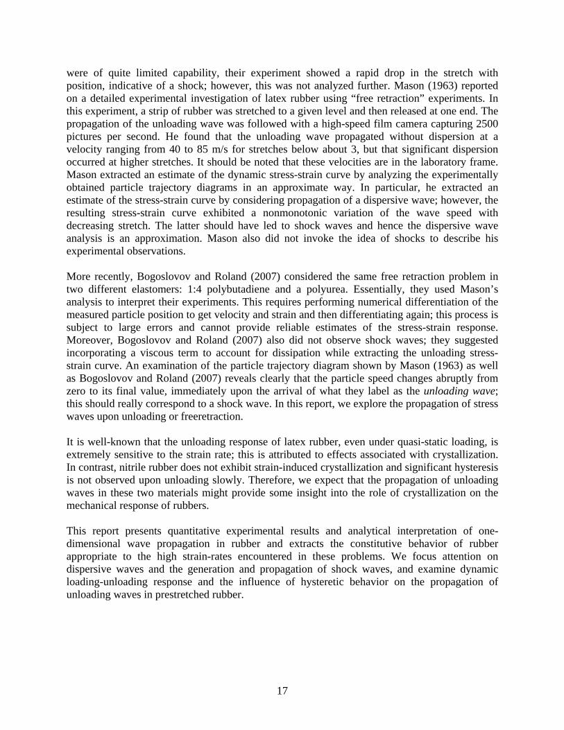
17

were of quite limited capability, their experiment showed a rapid drop in the stretch with position, indicative of a shock; however, this was not analyzed further. Mason (1963) reported on a detailed experimental investigation of latex rubber using “free retraction” experiments. In this experiment, a strip of rubber was stretched to a given level and then released at one end. The propagation of the unloading wave was followed with a high-speed film camera capturing 2500 pictures per second. He found that the unloading wave propagated without dispersion at a velocity ranging from 40 to 85 m/s for stretches below about 3, but that significant dispersion occurred at higher stretches. It should be noted that these velocities are in the laboratory frame. Mason extracted an estimate of the dynamic stress-strain curve by analyzing the experimentally obtained particle trajectory diagrams in an approximate way. In particular, he extracted an estimate of the stress-strain curve by considering propagation of a dispersive wave; however, the resulting stress-strain curve exhibited a nonmonotonic variation of the wave speed with decreasing stretch. The latter should have led to shock waves and hence the dispersive wave analysis is an approximation. Mason also did not invoke the idea of shocks to describe his experimental observations. More recently, Bogoslovov and Roland (2007) considered the same free retraction problem in two different elastomers: 1:4 polybutadiene and a polyurea. Essentially, they used Mason’s analysis to interpret their experiments. This requires performing numerical differentiation of the measured particle position to get velocity and strain and then differentiating again; this process is subject to large errors and cannot provide reliable estimates of the stress-strain response. Moreover, Bogoslovov and Roland (2007) also did not observe shock waves; they suggested incorporating a viscous term to account for dissipation while extracting the unloading stress-strain curve. An examination of the particle trajectory diagram shown by Mason (1963) as well as Bogoslovov and Roland (2007) reveals clearly that the particle speed changes abruptly from zero to its final value, immediately upon the arrival of what they label as the unloading wave; this should really correspond to a shock wave. In this report, we explore the propagation of stress waves upon unloading or freeretraction. It is well-known that the unloading response of latex rubber, even under quasi-static loading, is extremely sensitive to the strain rate; this is attributed to effects associated with crystallization. In contrast, nitrile rubber does not exhibit strain-induced crystallization and significant hysteresis is not observed upon unloading slowly. Therefore, we expect that the propagation of unloading waves in these two materials might provide some insight into the role of crystallization on the mechanical response of rubbers. This report presents quantitative experimental results and analytical interpretation of one-dimensional wave propagation in rubber and extracts the constitutive behavior of rubber appropriate to the high strain-rates encountered in these problems. We focus attention on dispersive waves and the generation and propagation of shock waves, and examine dynamic loading-unloading response and the influence of hysteretic behavior on the propagation of unloading waves in prestretched rubber.

18

We begin by first examining the structure of rubber and the constitutive behavior at the macroscopic scale in Chapter 2. The equations governing one-dimensional wave propagation in nonlinear materials and the general dynamic solutions of these equations are discussed in Chapter 3. The details of the experimental arrangement and the results of the investigation of tensile loading, finite amplitude waves in rubber are presented in Chapter 4. Experiments aimed at generating shocks in rubbers, and their interpretations in terms of the shock theory are described in Chapter 5. A description of free-retraction experiments in latex and nitrile rubber specimens is provided in Chapter 6. Analysis of these experiments yields the dynamic, hysteretic stress-strain response of the rubbers evaluated in this chapter. Finally, an experiment that generates a stationary phase front is described, and the results are presented in Chapter 7. We then summarize the response of rubber to dynamic loading and unloading conditions in Chapter 8.

19

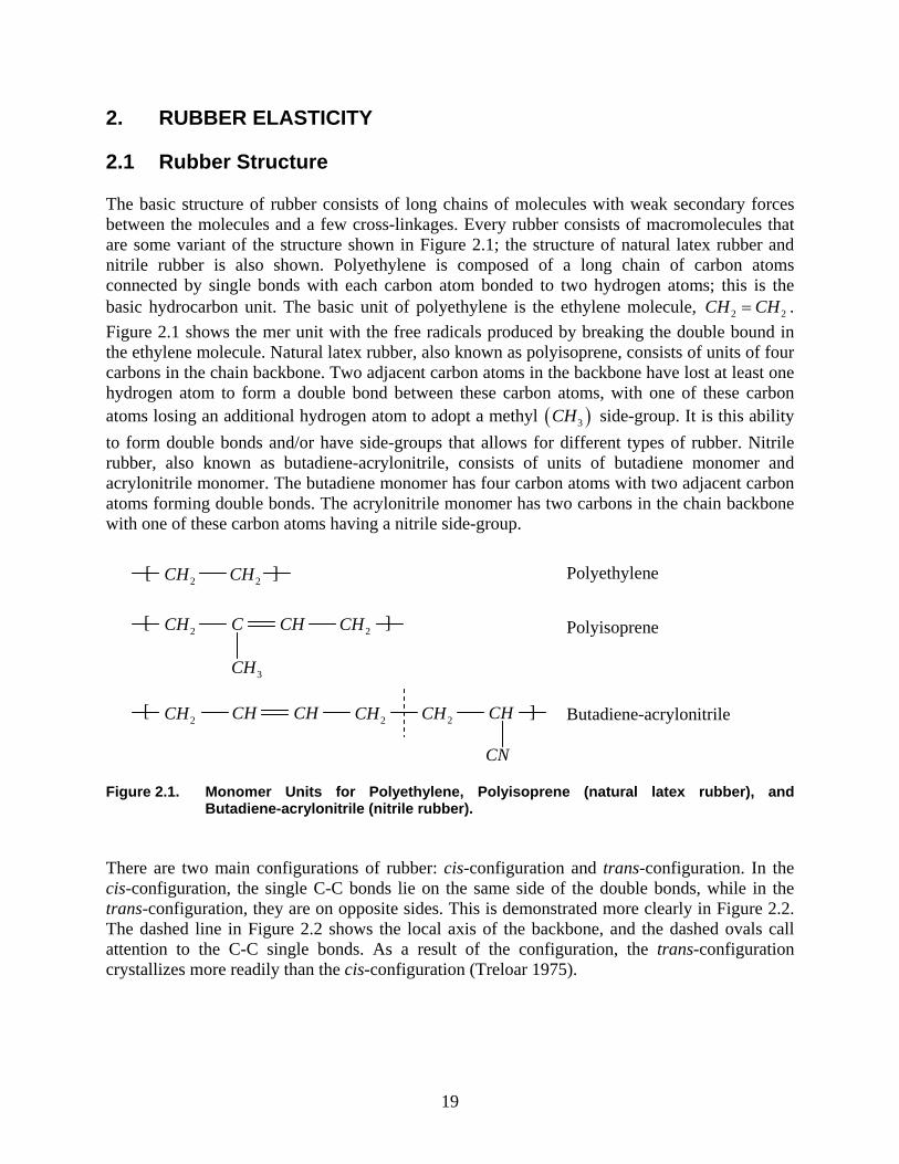
2. RUBBER ELASTICITY 2.1 Rubber Structure The basic structure of rubber consists of long chains of molecules with weak secondary forces between the molecules and a few cross-linkages. Every rubber consists of macromolecules that are some variant of the structure shown in Figure 2.1; the structure of natural latex rubber and nitrile rubber is also shown. Polyethylene is composed of a long chain of carbon atoms connected by single bonds with each carbon atom bonded to two hydrogen atoms; this is the basic hydrocarbon unit. The basic unit of polyethylene is the ethylene molecule, 2 2CH CH= . Figure 2.1 shows the mer unit with the free radicals produced by breaking the double bound in the ethylene molecule. Natural latex rubber, also known as polyisoprene, consists of units of four carbons in the chain backbone. Two adjacent carbon atoms in the backbone have lost at least one hydrogen atom to form a double bond between these carbon atoms, with one of these carbon atoms losing an additional hydrogen atom to adopt a methyl ( )3CH side-group. It is this ability to form double bonds and/or have side-groups that allows for different types of rubber. Nitrile rubber, also known as butadiene-acrylonitrile, consists of units of butadiene monomer and acrylonitrile monomer. The butadiene monomer has four carbon atoms with two adjacent carbon atoms forming double bonds. The acrylonitrile monomer has two carbons in the chain backbone with one of these carbon atoms having a nitrile side-group.

Figure 2.1. Monomer Units for Polyethylene, Polyisoprene (natural latex rubber), and

Butadiene-acrylonitrile (nitrile rubber). There are two main configurations of rubber: cis-configuration and trans-configuration. In the cis-configuration, the single C-C bonds lie on the same side of the double bonds, while in the trans-configuration, they are on opposite sides. This is demonstrated more clearly in Figure 2.2. The dashed line in Figure 2.2 shows the local axis of the backbone, and the dashed ovals call attention to the C-C single bonds. As a result of the configuration, the trans-configuration crystallizes more readily than the cis-configuration (Treloar 1975).

2CH 2CH

2CH C

3CH

CH 2CH

2CH CH

CN

CH 2CH 2CH CH

Polyethylene

Polyisoprene

Butadiene-acrylonitrile

[

[

[

]

]

]

20

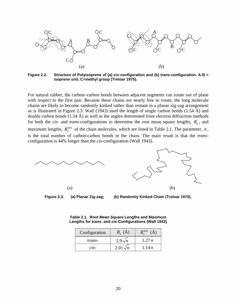
Figure 2.2. Structure of Polyisoprene of (a) cis-configuration and (b) trans-configuration. A-B =

isoprene unit. C=methyl group (Treloar 1975). For natural rubber, the carbon–carbon bonds between adjacent segments can rotate out of plane with respect to the first pair. Because these chains are nearly free to rotate, the long molecule chains are likely to become randomly kinked rather than remain in a planar zig-zag arrangement as is illustrated in Figure 2.3. Wall (1943) used the length of single carbon bonds (1.54 Å) and double carbon bonds (1.34 Å) as well as the angles determined from electron diffraction methods for both the cis- and trans-configurations to determine the root mean square lengths, nR , and maximum lengths, max

nR of the chain molecules, which are listed in Table 2.1. The parameter, n , is the total number of carbon-carbon bonds in the chain. The main result is that the trans-configuration is 44% longer than the cis-configuration (Wall 1943).

Figure 2.3. (a) Planar Zig-zag; (b) Randomly Kinked Chain (Treloar 1975).

Table 2.1. Root Mean Square Lengths and Maximum Lengths for trans- and cis-Configurations (Wall 1943)

Configuration nR (Å) maxnR (Å)

trans- 2.9 n 1.27 n cis- 2.01 n 1.14 n

C C C

A

B

C C

C

A B

(a) (b)

(a) (b)

21

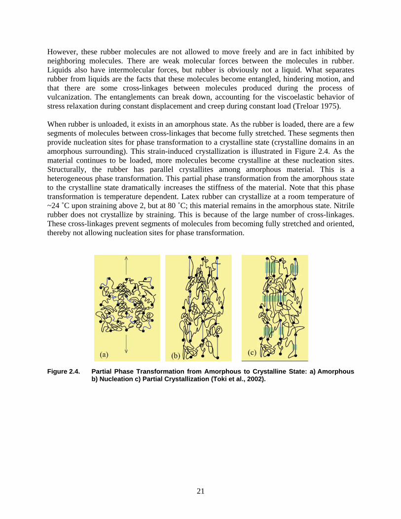
However, these rubber molecules are not allowed to move freely and are in fact inhibited by neighboring molecules. There are weak molecular forces between the molecules in rubber. Liquids also have intermolecular forces, but rubber is obviously not a liquid. What separates rubber from liquids are the facts that these molecules become entangled, hindering motion, and that there are some cross-linkages between molecules produced during the process of vulcanization. The entanglements can break down, accounting for the viscoelastic behavior of stress relaxation during constant displacement and creep during constant load (Treloar 1975). When rubber is unloaded, it exists in an amorphous state. As the rubber is loaded, there are a few segments of molecules between cross-linkages that become fully stretched. These segments then provide nucleation sites for phase transformation to a crystalline state (crystalline domains in an amorphous surrounding). This strain-induced crystallization is illustrated in Figure 2.4. As the material continues to be loaded, more molecules become crystalline at these nucleation sites. Structurally, the rubber has parallel crystallites among amorphous material. This is a heterogeneous phase transformation. This partial phase transformation from the amorphous state to the crystalline state dramatically increases the stiffness of the material. Note that this phase transformation is temperature dependent. Latex rubber can crystallize at a room temperature of ~24 ˚C upon straining above 2, but at 80 ˚C; this material remains in the amorphous state. Nitrile rubber does not crystallize by straining. This is because of the large number of cross-linkages. These cross-linkages prevent segments of molecules from becoming fully stretched and oriented, thereby not allowing nucleation sites for phase transformation.

Figure 2.4. Partial Phase Transformation from Amorphous to Crystalline State: a) Amorphous

b) Nucleation c) Partial Crystallization (Toki et al., 2002).

22

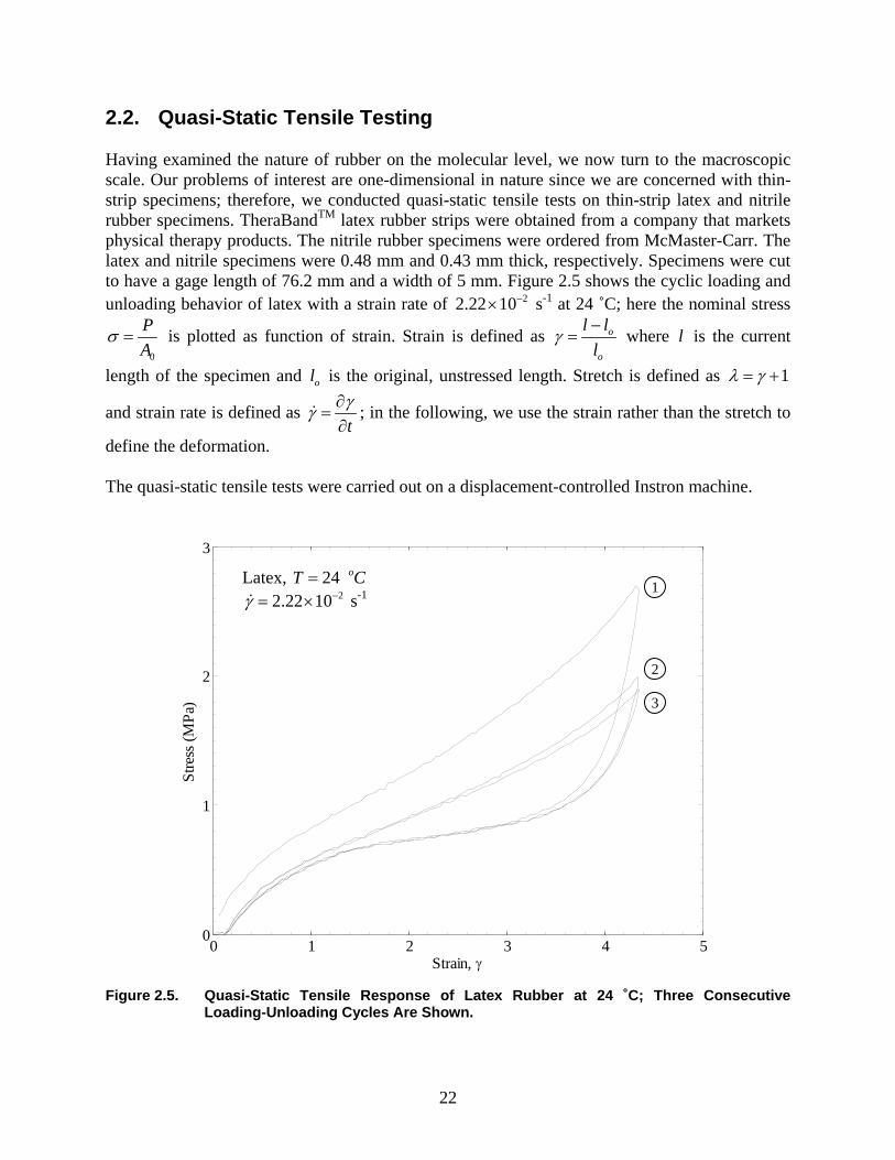
2.2. Quasi-Static Tensile Testing Having examined the nature of rubber on the molecular level, we now turn to the macroscopic scale. Our problems of interest are one-dimensional in nature since we are concerned with thin-strip specimens; therefore, we conducted quasi-static tensile tests on thin-strip latex and nitrile rubber specimens. TheraBandTM latex rubber strips were obtained from a company that markets physical therapy products. The nitrile rubber specimens were ordered from McMaster-Carr. The latex and nitrile specimens were 0.48 mm and 0.43 mm thick, respectively. Specimens were cut to have a gage length of 76.2 mm and a width of 5 mm. Figure 2.5 shows the cyclic loading and unloading behavior of latex with a strain rate of 22.22 10−× s-1 at 24 ˚C; here the nominal stress

0

PA

σ = is plotted as function of strain. Strain is defined as o

o

l ll

γ −= where l is the current

length of the specimen and ol is the original, unstressed length. Stretch is defined as 1λ γ= +

and strain rate is defined as tγγ ∂

=∂

; in the following, we use the strain rather than the stretch to

define the deformation. The quasi-static tensile tests were carried out on a displacement-controlled Instron machine.

Figure 2.5. Quasi-Static Tensile Response of Latex Rubber at 24 ˚C; Three Consecutive Loading-Unloading Cycles Are Shown.

0 1 2 3 4 50

1

2

3

Strain, γ

Stre

ss (M

Pa)

Latex, 24 oT C= 22.22 10γ −= × s-1

1

2

3

23

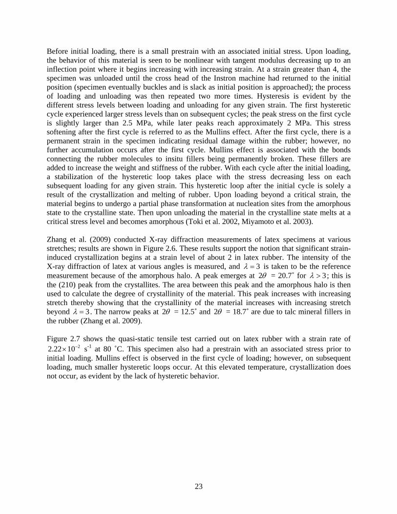
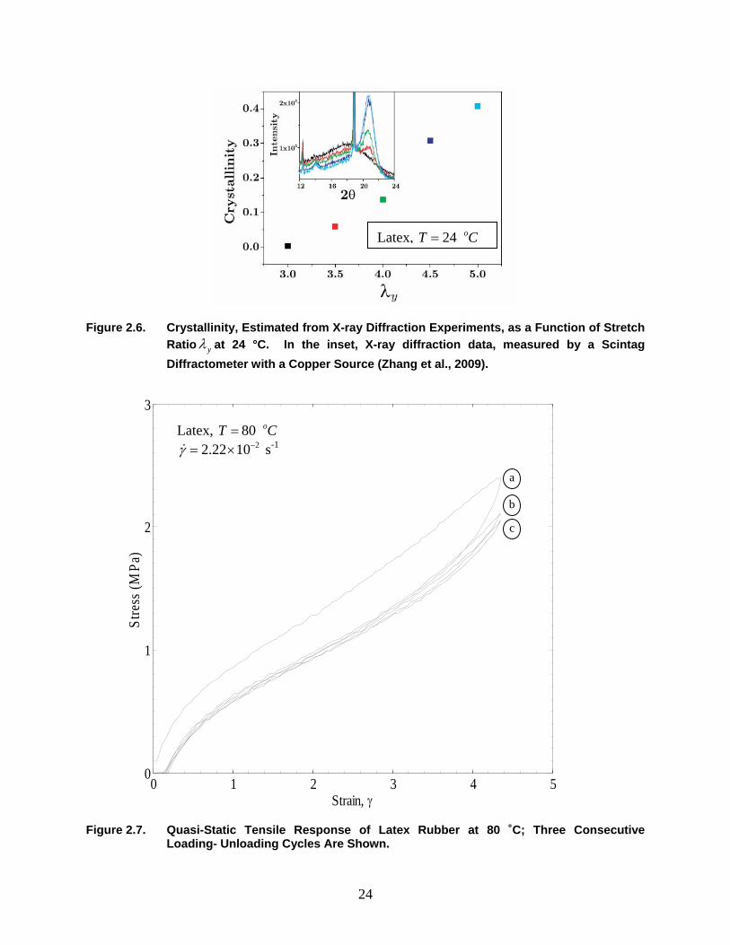
Before initial loading, there is a small prestrain with an associated initial stress. Upon loading, the behavior of this material is seen to be nonlinear with tangent modulus decreasing up to an inflection point where it begins increasing with increasing strain. At a strain greater than 4, the specimen was unloaded until the cross head of the Instron machine had returned to the initial position (specimen eventually buckles and is slack as initial position is approached); the process of loading and unloading was then repeated two more times. Hysteresis is evident by the different stress levels between loading and unloading for any given strain. The first hysteretic cycle experienced larger stress levels than on subsequent cycles; the peak stress on the first cycle is slightly larger than 2.5 MPa, while later peaks reach approximately 2 MPa. This stress softening after the first cycle is referred to as the Mullins effect. After the first cycle, there is a permanent strain in the specimen indicating residual damage within the rubber; however, no further accumulation occurs after the first cycle. Mullins effect is associated with the bonds connecting the rubber molecules to insitu fillers being permanently broken. These fillers are added to increase the weight and stiffness of the rubber. With each cycle after the initial loading, a stabilization of the hysteretic loop takes place with the stress decreasing less on each subsequent loading for any given strain. This hysteretic loop after the initial cycle is solely a result of the crystallization and melting of rubber. Upon loading beyond a critical strain, the material begins to undergo a partial phase transformation at nucleation sites from the amorphous state to the crystalline state. Then upon unloading the material in the crystalline state melts at a critical stress level and becomes amorphous (Toki et al. 2002, Miyamoto et al. 2003). Zhang et al. (2009) conducted X-ray diffraction measurements of latex specimens at various stretches; results are shown in Figure 2.6. These results support the notion that significant strain-induced crystallization begins at a strain level of about 2 in latex rubber. The intensity of the X-ray diffraction of latex at various angles is measured, and 3λ = is taken to be the reference measurement because of the amorphous halo. A peak emerges at 2θ = 20.7˚ for 3λ > ; this is the (210) peak from the crystallites. The area between this peak and the amorphous halo is then used to calculate the degree of crystallinity of the material. This peak increases with increasing stretch thereby showing that the crystallinity of the material increases with increasing stretch beyond 3λ = . The narrow peaks at 2θ = 12.5˚ and 2θ = 18.7˚ are due to talc mineral fillers in the rubber (Zhang et al. 2009). Figure 2.7 shows the quasi-static tensile test carried out on latex rubber with a strain rate of

22.22 10−× s-1 at 80 ˚C. This specimen also had a prestrain with an associated stress prior to initial loading. Mullins effect is observed in the first cycle of loading; however, on subsequent loading, much smaller hysteretic loops occur. At this elevated temperature, crystallization does not occur, as evident by the lack of hysteretic behavior.

24

Figure 2.6. Crystallinity, Estimated from X-ray Diffraction Experiments, as a Function of Stretch

Ratio yλ at 24 °C. In the inset, X-ray diffraction data, measured by a Scintag Diffractometer with a Copper Source (Zhang et al., 2009).

Figure 2.7. Quasi-Static Tensile Response of Latex Rubber at 80 ˚C; Three Consecutive

Loading- Unloading Cycles Are Shown.

0 1 2 3 4 50

1

2

3

Strain, γ

Stre

ss (M

Pa)

Latex, 80 oT C= 22.22 10γ −= × s-1

a

b

c

Latex, 24 oT C=

25

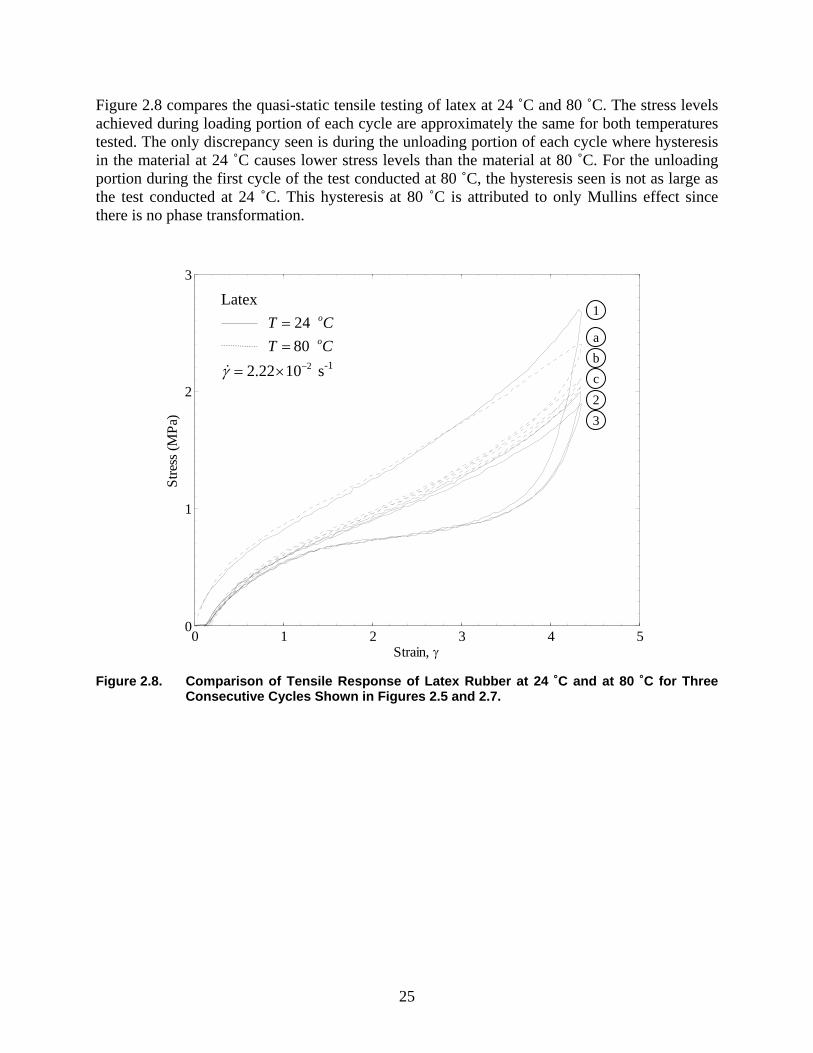
Figure 2.8 compares the quasi-static tensile testing of latex at 24 ˚C and 80 ˚C. The stress levels achieved during loading portion of each cycle are approximately the same for both temperatures tested. The only discrepancy seen is during the unloading portion of each cycle where hysteresis in the material at 24 ˚C causes lower stress levels than the material at 80 ˚C. For the unloading portion during the first cycle of the test conducted at 80 ˚C, the hysteresis seen is not as large as the test conducted at 24 ˚C. This hysteresis at 80 ˚C is attributed to only Mullins effect since there is no phase transformation.

Figure 2.8. Comparison of Tensile Response of Latex Rubber at 24 ˚C and at 80 ˚C for Three

Consecutive Cycles Shown in Figures 2.5 and 2.7.

0 1 2 3 4 50

1

2

3

Strain, γ

Stre

ss (M

Pa)

80 oT C=

Latex 24 oT C=

22.22 10γ −= × s-1

1

2 3

a b c

26

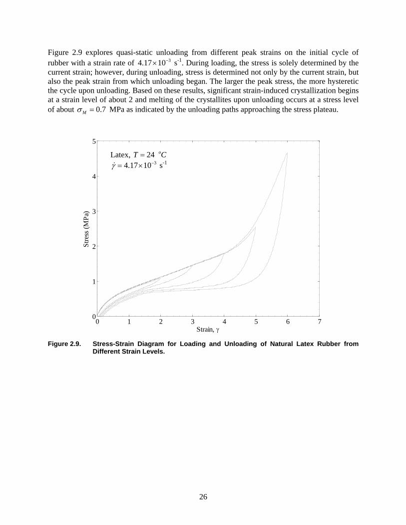
Figure 2.9 explores quasi-static unloading from different peak strains on the initial cycle of rubber with a strain rate of 34.17 10−× s-1. During loading, the stress is solely determined by the current strain; however, during unloading, stress is determined not only by the current strain, but also the peak strain from which unloading began. The larger the peak stress, the more hysteretic the cycle upon unloading. Based on these results, significant strain-induced crystallization begins at a strain level of about 2 and melting of the crystallites upon unloading occurs at a stress level of about 0.7Mσ = MPa as indicated by the unloading paths approaching the stress plateau.

Figure 2.9. Stress-Strain Diagram for Loading and Unloading of Natural Latex Rubber from

Different Strain Levels.

0 1 2 3 4 5 6 70

1

2

3

4

5

Strain, γ

Stre

ss (M

Pa)

Latex, 24 oT C= 34.17 10γ −= × s-1

27

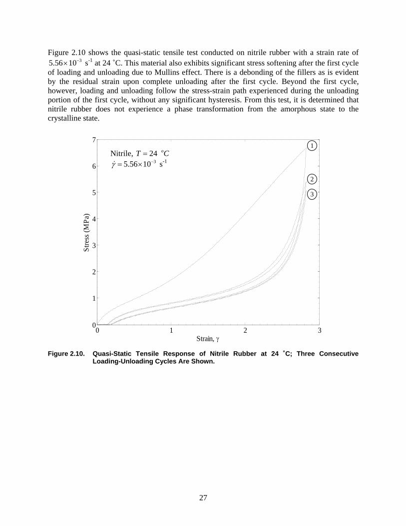
Figure 2.10 shows the quasi-static tensile test conducted on nitrile rubber with a strain rate of 35.56 10−× s-1 at 24 ˚C. This material also exhibits significant stress softening after the first cycle

of loading and unloading due to Mullins effect. There is a debonding of the fillers as is evident by the residual strain upon complete unloading after the first cycle. Beyond the first cycle, however, loading and unloading follow the stress-strain path experienced during the unloading portion of the first cycle, without any significant hysteresis. From this test, it is determined that nitrile rubber does not experience a phase transformation from the amorphous state to the crystalline state.

Figure 2.10. Quasi-Static Tensile Response of Nitrile Rubber at 24 ˚C; Three Consecutive

Loading-Unloading Cycles Are Shown.

0 1 2 30

1

2

3

4

5

6

7

Strain, γ

Stre

ss (M

Pa)

Nitrile, 24 oT C= 35.56 10γ −= × s-1

1

2

3

28

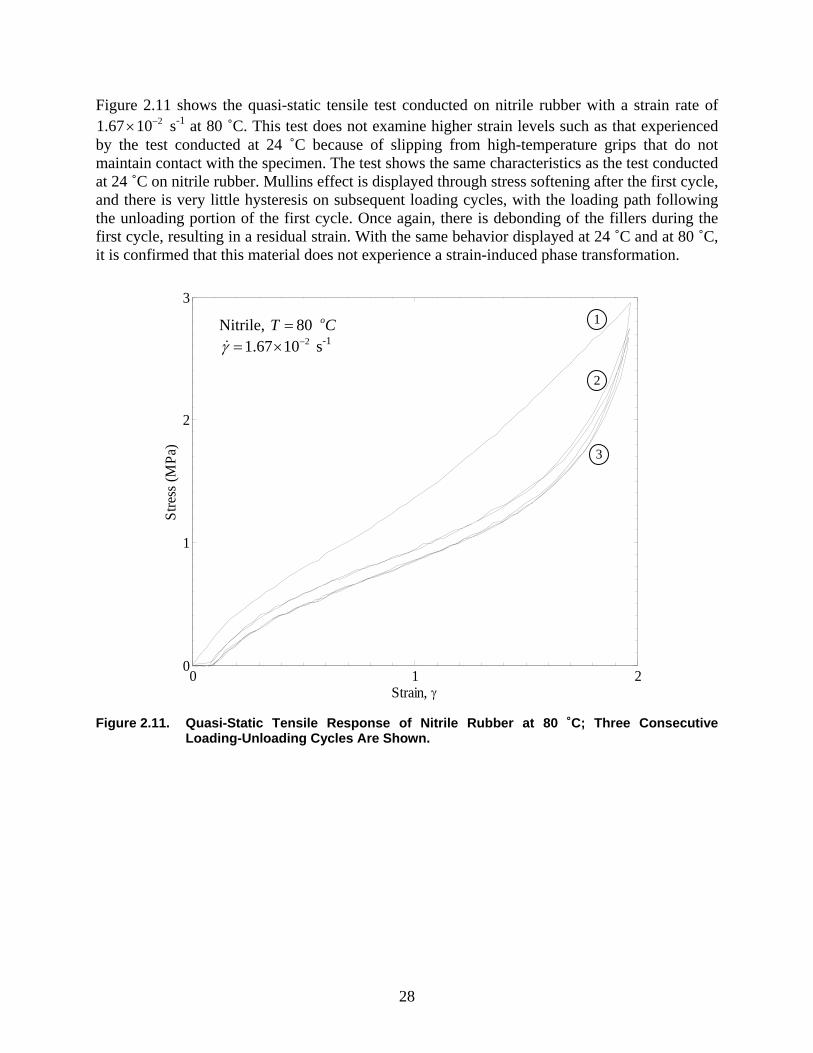
Figure 2.11 shows the quasi-static tensile test conducted on nitrile rubber with a strain rate of 21.67 10−× s-1 at 80 ˚C. This test does not examine higher strain levels such as that experienced

by the test conducted at 24 ˚C because of slipping from high-temperature grips that do not maintain contact with the specimen. The test shows the same characteristics as the test conducted at 24 ˚C on nitrile rubber. Mullins effect is displayed through stress softening after the first cycle, and there is very little hysteresis on subsequent loading cycles, with the loading path following the unloading portion of the first cycle. Once again, there is debonding of the fillers during the first cycle, resulting in a residual strain. With the same behavior displayed at 24 ˚C and at 80 ˚C, it is confirmed that this material does not experience a strain-induced phase transformation.

Figure 2.11. Quasi-Static Tensile Response of Nitrile Rubber at 80 ˚C; Three Consecutive

Loading-Unloading Cycles Are Shown.

0 1 20

1

2

3

Strain, γ

Stre

ss (M

Pa)

Nitrile, 80 oT C= 21.67 10γ −= × s-1

1

2

3

29

2.3. Material Models In the past, the quasi-static testing of rubber materials has been examined quite thoroughly, and several models have been proposed for the loading of rubber-like materials. We focus on phenomenological models. One such model is the Mooney-Rivlin model (Treloar 1975). This model assumes that the material is incompressible, isotropic in the unstrained state, and the strain energy is dependent on even powers of stretch. The strain invariants are as follows:

2 2 21 1 2 3

2 2 2 2 2 22 1 2 2 3 3 1

2 2 23 1 2 3 1,

I

I

I

= + +

= + +

= =

λ λ λ

λ λ λ λ λ λ

λ λ λ

(2-1)

where 1 2 3, ,λ λ λ are the principal stretches and the last equation enforces incompressibility. Eliminating 3I , we have just two strain invariants,

2 21 1 2 2 2

1 2

2 22 1 22 2

1 2

1

1 1 .

I

I

= + +

= + +

λ λλ λ

λ λλ λ

(2-2)

The strain energy function is then written as

( ) ( )1 20, 0

3 3i jij

i jW C I I

∞

= =

= − −∑ . (2-3)

The Mooney-Rivlin equation is then arrived at using just 10C and 01C as the only nonzero constants:

( ) ( )10 1 01 23 3W C I C I= − + − . (2-4)

If we then applies this to a simple elongation such as the uniaxial tension test, we find that the transverse stretches, and stresses must observe 2 2 1

2 3λ λ λ −= = and 2 3 0σ σ= = with 1λ λ= , such that the constitutive relation is

2

1 2

1 12 W WI I

σ λλ λ

⎛ ⎞∂ ∂⎛ ⎞= − +⎜ ⎟⎜ ⎟ ∂ ∂⎝ ⎠⎝ ⎠. (2-5)

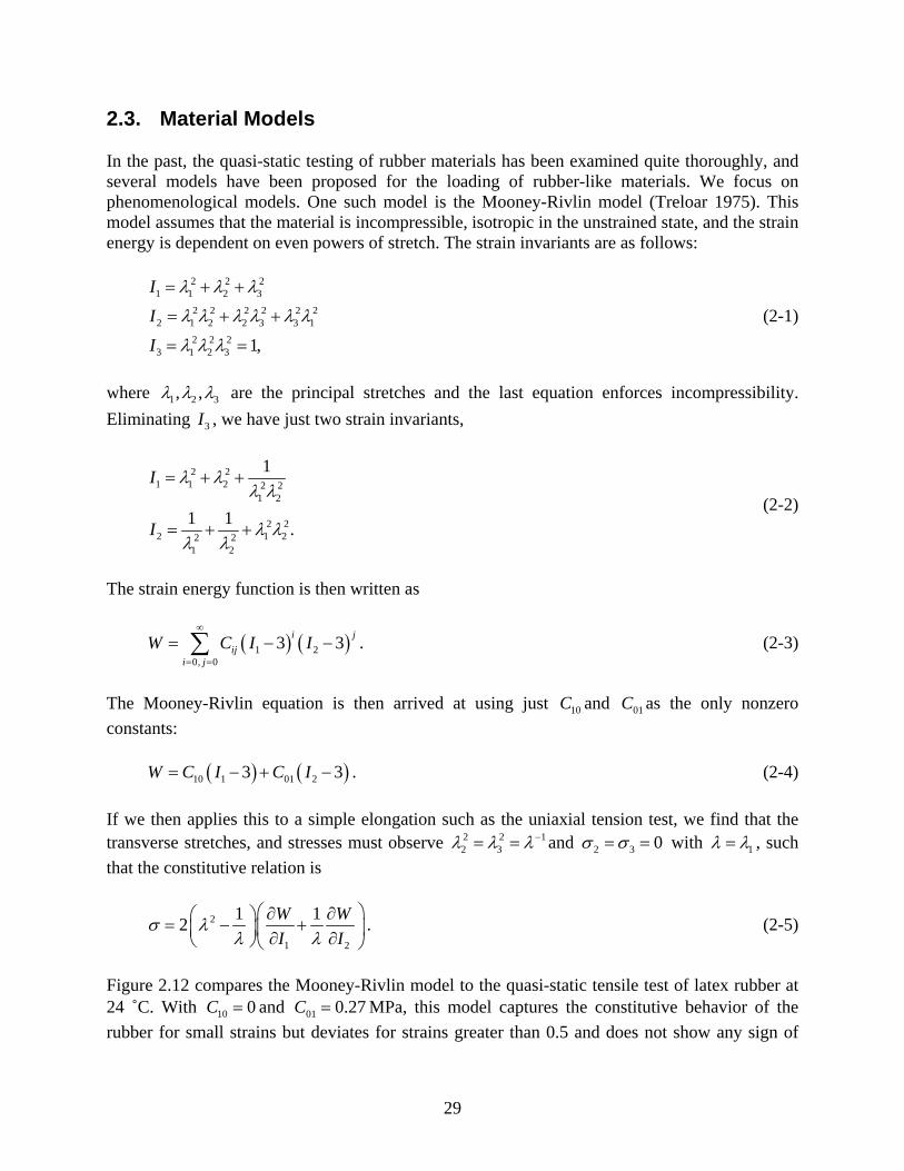
Figure 2.12 compares the Mooney-Rivlin model to the quasi-static tensile test of latex rubber at 24 ˚C. With 10 0C = and 01 0.27C = MPa, this model captures the constitutive behavior of the rubber for small strains but deviates for strains greater than 0.5 and does not show any sign of

30

increasing stiffness for large strains. With 10 0.07C = MPa and 01 0.18C = MPa, the model also captures small strain constitutive behavior and shows stiffening for larger strains. Neither fit can capture the stress values beyond small strains; for this, we need more parameters. Knowles (2002) suggested modeling the response of rubber qualitatively with a cubic stress-strain law; while this is not an appropriate model that may be generalized easily either to compression or to three-dimensional problems, it enables easy analytical solutions to the impact induced tensile wave problem and captures the essence of the change from the concave to convex response of the material. In particular, the nonlinear response of rubber for the uniaxial stretching of rubber may then be represented as follows,

( ) ( )γγγγσ ++= 22

33 aaE , (2-6)

where 3a and 2a are constants and E is the modulus of elasticity for infinitesimal deformations,

Figure 2.12. Comparison of Mooney-Rivlin Model to Latex Quasi-Static Test Data (Black Line).

Blue Dashed Line Corresponds to 10 0C = MPa and 01 0.27C = MPa. Blue Dash-Dot

Line Corresponds to 10 0.07C = MPa and 01 0.18C = MPa.

0 1 2 3 4 5 60

1

2

3

4

5

6

Strain, γ

Stre

ss, σ

(MPa

)

Latex, 24 oT C=

10 010 , 0.27C C= = MPa

10 010 , 0.27C C= = MPa

Quasi-Static

22.22 10γ −= × s-1

Mooney-Rivlin

31

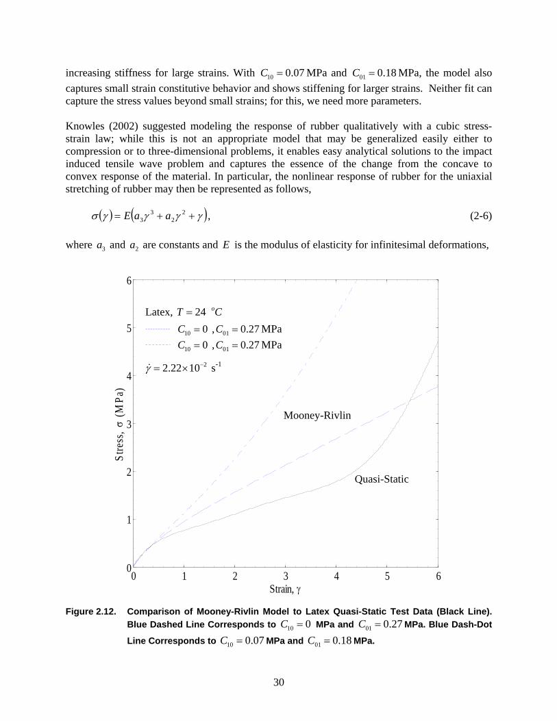
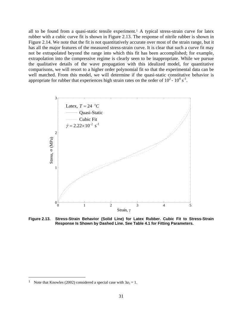
all to be found from a quasi-static tensile experiment.1 A typical stress-strain curve for latex rubber with a cubic curve fit is shown in Figure 2.13. The response of nitrile rubber is shown in Figure 2.14. We note that the fit is not quantitatively accurate over most of the strain range, but it has all the major features of the measured stress-strain curve. It is clear that such a curve fit may not be extrapolated beyond the range into which this fit has been accomplished; for example, extrapolation into the compressive regime is clearly seen to be inappropriate. While we pursue the qualitative details of the wave propagation with this idealized model, for quantitative comparisons, we will resort to a higher order polynomial fit so that the experimental data can be well matched. From this model, we will determine if the quasi-static constitutive behavior is appropriate for rubber that experiences high strain rates on the order of 102 - 104 s-1.

Figure 2.13. Stress-Strain Behavior (Solid Line) for Latex Rubber. Cubic Fit to Stress-Strain

Response Is Shown by Dashed Line. See Table 4.1 for Fitting Parameters.

1 Note that Knowles (2002) considered a special case with 3a3 = 1.

0 1 2 3 4 50

1

2

3

Strain, γ

Stre

ss, σ

(MPa

)

Latex, 24 oT C= Quasi-Static Cubic Fit

22.22 10γ −= × s-1

32

Figure 2.14. Stress-Strain Behavior (Solid Line) for Nitrile Rubber. Cubic Fit to the Stress-Strain

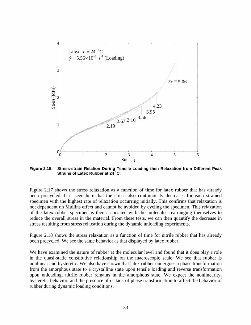
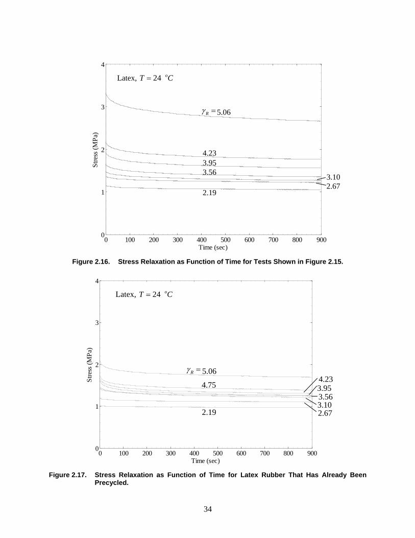
Response Is Shown by Dashed Line. See Table 4.1 for Fitting Parameters. 2.4. Relaxation At this point, we examine the stress relaxation in latex rubber. The relaxation tests are carried out to better understand what the stress levels are prior to dynamic unloading. In some of the dynamic experiments conducted, the material is held at large strains for a few tens of seconds prior to dynamic loading, and we wish to quantify the decrease in stress. Figure 2.15 shows the relaxation tests carried out on latex rubber at 24 ˚C where Mullins effect has not been removed. In this test, the specimen is stretched at a strain rate of 35.56 10−× s-1. At the desired maximum strain, the strain is held constant for 15 minutes. In each test conducted, there is stress relaxation. As can be seen with larger peak strains, there is larger stress relaxation in the same duration. Figure 2.16 shows just the stress relaxation as a function of time. The stress decreases at the fastest rate at the beginning of relaxation. The stress continues to decrease during the entire relaxation test.

0 1 2 30

1

2

3

4

5

Strain, γ

Stre

ss, σ

(MPa

)Nitrile, 24 oT C=

Quasi-Static Cubic Fit

35.56 10γ −= × s-1

33

Figure 2.15. Stress-strain Relation During Tensile Loading then Relaxation from Different Peak

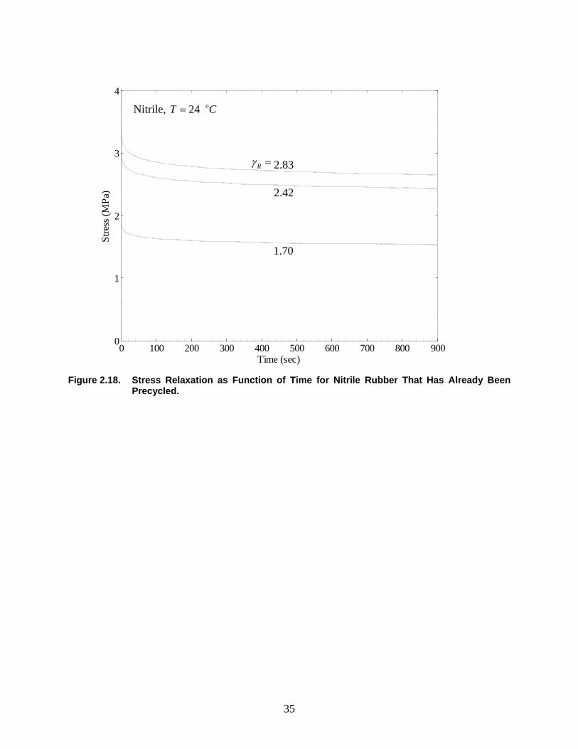
Strains of Latex Rubber at 24 ˚C. Figure 2.17 shows the stress relaxation as a function of time for latex rubber that has already been precycled. It is seen here that the stress also continuously decreases for each strained specimen with the highest rate of relaxation occurring initially. This confirms that relaxation is not dependent on Mullins effect and cannot be avoided by cycling the specimen. This relaxation of the latex rubber specimen is then associated with the molecules rearranging themselves to reduce the overall stress in the material. From these tests, we can then quantify the decrease in stress resulting from stress relaxation during the dynamic unloading experiments. Figure 2.18 shows the stress relaxation as a function of time for nitrile rubber that has already been precycled. We see the same behavior as that displayed by latex rubber. We have examined the nature of rubber at the molecular level and found that it does play a role in the quasi-static constitutive relationship on the macroscopic scale. We see that rubber is nonlinear and hysteretic. We also have shown that latex rubber undergoes a phase transformation from the amorphous state to a crystalline state upon tensile loading and reverse transformation upon unloading; nitrile rubber remains in the amorphous state. We expect the nonlinearity, hysteretic behavior, and the presence of or lack of phase transformation to affect the behavior of rubber during dynamic loading conditions.

0 1 2 3 4 5 60

1

2

3

4

Strain, γ

Stre

ss (M

Pa)

Latex, 24 oT C= 35.56 10γ −= × s-1 (Loading)

2.19 2.67 3.10 3.56

3.95 4.23

Rγ = 5.06

34

Figure 2.16. Stress Relaxation as Function of Time for Tests Shown in Figure 2.15.

Figure 2.17. Stress Relaxation as Function of Time for Latex Rubber That Has Already Been

Precycled.

0 100 200 300 400 500 600 700 800 9000

1

2

3

4

Time (sec)

Stre

ss (M

Pa)

Latex, 24 oT C=

Rγ = 5.06

4.23 3.95 3.56 3.10

2.67 2.19

0 100 200 300 400 500 600 700 800 9000

1

2

3

4

Time (sec)

Stre

ss (M

Pa)

Latex, 24 oT C=

Rγ = 5.06

4.754.23 3.95 3.56 3.10 2.67 2.19

35

Figure 2.18. Stress Relaxation as Function of Time for Nitrile Rubber That Has Already Been

Precycled.

0 100 200 300 400 500 600 700 800 9000

1

2

3

4

Time (sec)

Stre

ss (M

Pa)

Nitrile, 24 oT C=

Rγ = 2.83

2.42

1.70

36

3. THEORY OF ONE-DIMENSIONAL WAVE PROPAGATION In this chapter, the general equations of motion and the general solutions for one-dimensional wave motion in nonlinear materials are discussed. The particular case of a cubic material model is considered to specialize the formulation to rubbers and elastomers. 3.1 Equations of Motion Consider a one-dimensional, semi-infinite strip of rubber occupying 0 x≤ < ∞ , where x represents the position of a material point in the reference configuration. At 0t = , the end 0x = is subjected to a constant velocity V− in the x-direction; this generates a tensile wave propagating into the material in the x-direction. If the transverse dimensions of the rubber strip are small, inertia effects associated with the transverse motion may be neglected,2 and one may assume one-dimensional motion of the rubber strip. Under such conditions, the subsequent motion of material points in the strip is represented only by ),( txu , the displacement in the x-direction; therefore, the current position of the material point x at any time t is given by

( , ) ( , )y x t x u x t= + . The corresponding strain and particle velocity are given by ( , )x t u xγ = ∂ ∂ and ( , )v x t u t= ∂ ∂ respectively. The stretch corresponding to this strain is 1 ( , )x tλ γ= + . The governing equations of motion for this one-dimensional wave problem in a nonlinearly elastic material are obtained from the balance of linear momentum and kinematic compatibility:

( )

,

vx tvx t

∂ ∂′ =∂ ∂∂ ∂

=∂ ∂

γσ γ ρ

γ (3-1)

where ρ is the mass density, ( )γσ is the nonlinear stress-strain relationship appropriate to this one-dimensional problem for the material, and the prime indicates a derivative with respect to the argument. Equation (3-1) can be expressed in terms of the particle displacement to obtain the nonlinear wave equation in familiar form:

( )2 22

2 2u uc

x tγ ∂ ∂⎡ ⎤ =⎣ ⎦ ∂ ∂

, (3-2)

where ( ) ( )c γ σ γ ρ′= is the speed (in reference configuration) of incremental waves propagating in a specimen strained to a level γ . Suitable initial conditions need to be specified; for example, the initial strain and particle velocity along the specimen can be prescribed as

( ,0) ( )x g xγ = , ( ,0) ( )v x h x= .

2 See Graff (1975) for higher-order theories such as Love-Rayleigh rod theory or the Pochhammer-Chree model to

account for this in linearly elastic materials.

37

3.2 General Solutions for a Semi-infinite Strip Now let us consider the general solutions to the tensile impact problem for the semi-infinite strip; for this problem, we have the boundary condition (0, )v t V= − with the initial conditions

0( ,0)xγ γ= , ( ,0) 0v x = . For this boundary-initial value problem, it is clear that there is neither a characteristic length scale nor a characteristic time scale; therefore, all solutions to this problem must scale as tx=ξ . Also, the tx − plane is divided into sectors, with two kinds of possible sectors — fan sectors corresponding to dispersive waves with ( )ξγγ ˆ),( =tx and ( )ξvtxv ˆ),( = , and constant sectors with ( , )x tγ γ= = const and ( , )v x t v= = const. Theoretical considerations are conducted in reference configuration, so we refer to the tx − plane. Experimental measurements will be made in laboratory coordinates so that the results will be presented in the y t− plane.

3.2.1 Fan Solution In the fan sector, introducing a change of variables from x and t to ξ in the equation of motion, we can show that

ξξγ =))(ˆ(c , ( ) ( )ξγξξ ′−=′ ˆv̂ . (3-3)

Then, the particle velocity at any point in the fan sector can be found by integrating the second of Eq. (3-3) from the beginning of the fan sector at 1ξ :

( ) ( ) ( ) ( )( )

( )

1 1

1 ˆˆ ˆv v d c dγ ξξ

ξ γ ξ

ξ ξ ζγ ζ ζ ζ ζ′− = − = −∫ ∫ . (3-4)

A change of variable from ξ to γ has been effected in the second integral in Eq. (3-4). 1ξ is the wave speed corresponding to the initial point of the fan sector. Thus, in the fan sector, at any ξ the strain is obtained by inverting the first of Eq. (3-3) and the particle velocity is obtained from the integral in the second of Eq. (3-4). The particle displacement can also be determined either by integrating the strain along x at fixed t :

1 1

1 ˆ( , ) ( , ) ( , ) ( )x

t

u x t u t t x t dx t dξ

ξ ξ

ξ γ γ ζ ζ− = =∫ ∫ (3-5)

or by integrating the particle velocity with respect to t at fixed x :

1 1

21 ˆ( , ) ( , ) ( , ) ( )

t

x

u x t u x x v x t dt x v dξ

ξ ξ

ξ ζ ζ ζ−− = = −∫ ∫ . (3-6)

The trajectory of a material point in the laboratory frame can then be calculated as ( , ) ( , )y x t x u x t= + .

38

3.2.2 Constant Solution It is obvious that ( , )x tγ γ= = const, and ( , )v x t v= = const, satisfy the equation of motion and compatibility condition; the appropriate constants must be determined so as to match the solutions at sector boundaries. Then the particle displacement can also be determined by integrating the strain along x at fixed t :

( )1

1 1( , ) ( , ) ( , )x

t

u x t u t t x t dx x tξ

ξ γ ξ γ− = = −∫ (3-7)

from the sector boundary 1ξ or by integrating the particle velocity with respect to t at fixed x :

( )1

1 1( , ) ( , ) ( , )t

x

u x t u x x v x t dt x t vξ

ξ ξ− = = −∫ . (3-8)

The trajectory of a material point in the laboratory frame can then be calculated as ( , ) ( , )y x t x u x t= + . This general solution can be evaluated for any given constitutive behavior;

this procedure is rather well established for materials that exhibit a concave stress-strain curve such as metallic alloys; for rubbers and elastomers that exhibit an inflection point with a switch from concave to convex stress-strain behavior, the possibility exists of tensile shocks. Such shocks correspond to two constant solutions separated by an abrupt jump and are discussed in Sections 3.5 and 3.6. 3.3 Solution by Method of Characteristics The general solution described in Section 3.2 is quite easily evaluated for a given constitutive model. For problems involving finite length specimens (as is inevitable in the experiments discussed), the similarity solution of Section 3.2 breaks down, and one must resort to other methods of solutions. The method of characteristics is a powerful technique for solving such problems. For the hyperbolic system in Eq.(3-1), the Riemann invariants can be shown to be

( )

( )

1

2

on

on .

dxr cv cdtdxr cv cdt

= + = −

= − + =

ρ σ

ρ σ (3-9)

For this problem, the Riemann invariants, ( ) ,kr are constant along the characteristics, c∓ . In implementing this method, we divide x-axis into discrete nodes and time into a series of time steps as illustrated in Figure 3.1. Here, k

ix denotes the node at i during time-step k. The time increment at each step is calculated such that the fastest wave speed from the previous time step satisfies the Courant-Friedrichs-Levy condition. In addition, kx− is the origin of the characteristic,

kc−− , that arrives at 1kix + and is located between nodes k

ix and 1kix + ; similarly, kx+ is the origin of

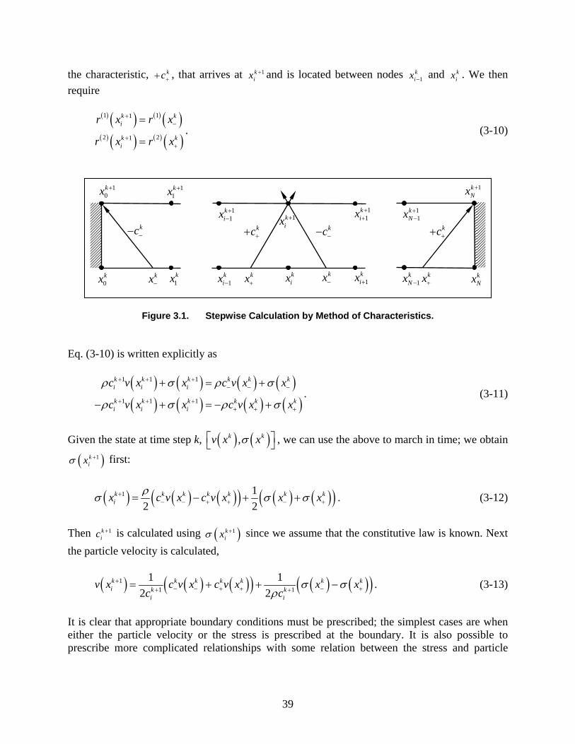
39

the characteristic, kc++ , that arrives at 1kix + and is located between nodes 1

kix − and k

ix . We then require

( ) ( ) ( ) ( )( ) ( ) ( ) ( )

1 11

2 21

k ki

k ki

r x r x

r x r x

+−

++

=

=. (3-10)

Figure 3.1. Stepwise Calculation by Method of Characteristics. Eq. (3-10) is written explicitly as

( ) ( ) ( ) ( )( ) ( ) ( ) ( )

1 1 1

1 1 1

k k k k k ki i i

k k k k k ki i i

c v x x c v x x

c v x x c v x x

ρ σ ρ σ

ρ σ ρ σ

+ + +− − −

+ + ++ + +

+ = +

− + = − +. (3-11)

Given the state at time step k, ( ) ( ),k kv x xσ⎡ ⎤⎣ ⎦ , we can use the above to march in time; we obtain

( )1kixσ + first:

( ) ( ) ( )( ) ( ) ( )( )1 12 2

k k k k k k kix c v x c v x x xρσ σ σ+

− − + + − += − + + . (3-12)

Then 1kic + is calculated using ( )1k

ixσ + since we assume that the constitutive law is known. Next the particle velocity is calculated,

( ) ( ) ( )( ) ( ) ( )( )11 1

1 12 2

k k k k k k ki k k

i i

v x c v x c v x x xc c

σ σρ

+− − + + − ++ += + + − . (3-13)

It is clear that appropriate boundary conditions must be prescribed; the simplest cases are when either the particle velocity or the stress is prescribed at the boundary. It is also possible to prescribe more complicated relationships with some relation between the stress and particle

0kx k

ix 1kix − 1

kix +

1kix +

11

kix ++ 1

1kix +−

kx− kx+

kc−− kc++

1kNx − k

Nx

1kNx +

11

kNx +

−

kx+

kc++

1kx

10kx +

kx−

kc−−

11kx +

40

velocity or displacement to simulate compliant boundaries or interfaces. For the left boundary (see Figure 3.1), we have

( ) ( ) ( ) ( )( ) ( ) ( ) ( )

1 110

1 1 10 0 0

k k

k k k k k k

r x r x

c v x x c v x xρ σ ρ σ

+−

+ + +− − −

=

+ = +. (3-14)

Similarly, for the right boundary (see Figure 3.1) we have,

( ) ( ) ( ) ( )( ) ( ) ( ) ( )

2 21

1 1 1 .

k kN

k k k k k kN N N

r x r x

c v x x c v x x

++

+ + ++ + +

=

− + = − +ρ σ ρ σ (3-15)

Since either the particle velocity or the stress is given at 10kx + and 1k

Nx + , the other quantity can be determined from Eqs. (3-8) and (3-15). The particle trajectory is then calculated as

( )1 1( )k k ki i iy x x v x dt+ += + with dt equal to the time step between 1k + and k . With this

procedure, we can deal with prescribed boundary conditions on either end of a finite strip of rubber. Therefore, given an appropriate constitutive relation, the method of characteristics can be used to determine the response of a finite length specimen. 3.4 Approximate Material Model for Rubber Knowles (2002) suggested modeling the response of rubber qualitatively with a cubic stress-strain law; while this is not an appropriate model that may be generalized easily to compression or to three-dimensional problems, it enables easy analytical solutions to the impact induced uniaxial tensile wave problem and captures the essence of the change from the concave to convex response of the material. In particular, the nonlinear response of rubber for the uniaxial stretching of rubber may then be represented as follows:

( ) ( )γγγγσ ++= 22

33 aaE , (3-16)

where 3a and 2a are constants and E is the modulus of elasticity for infinitesimal deformations, all to be found from a quasi-static tensile experiment.3 A typical stress-strain curve for latex rubber, with a cubic curve fit is shown in Figure 3.2a. The response of nitrile rubber is shown in Figure 3.2b. We note that the fit is not quantitatively accurate over most of the strain range, but it has all the major features of the measured stress-strain curve.

3 Note that Knowles (2002) considered a special case with 3a3 = 1.

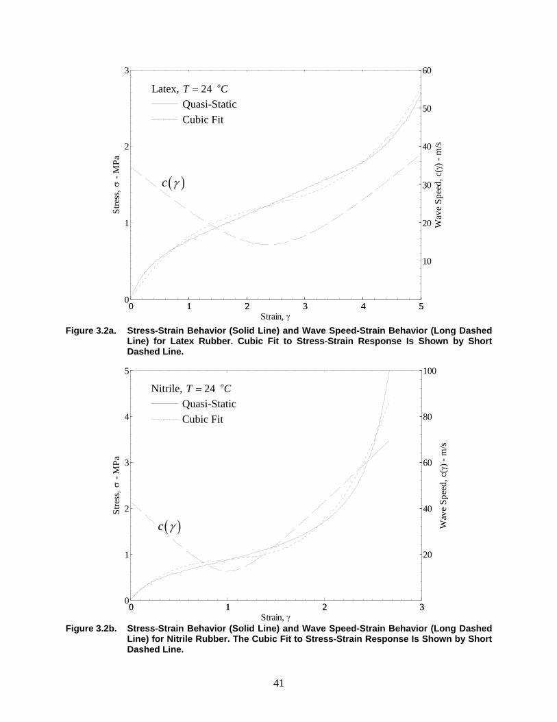
41

Figure 3.2a. Stress-Strain Behavior (Solid Line) and Wave Speed-Strain Behavior (Long Dashed

Line) for Latex Rubber. Cubic Fit to Stress-Strain Response Is Shown by Short Dashed Line.

Figure 3.2b. Stress-Strain Behavior (Solid Line) and Wave Speed-Strain Behavior (Long Dashed

Line) for Nitrile Rubber. The Cubic Fit to Stress-Strain Response Is Shown by Short Dashed Line.

0 1 2 3 4 50

1

2

3

Stre

ss, σ

- M

Pa

Strain, γ0 1 2 3 4 5

10

20

30

40

50

60

Wav

e Sp

eed,

c(γ

) - m

/s

Latex, 24 oT C= Quasi-Static Cubic Fit

( )c γ

0 1 2 30

1

2

3

4

5

Stre

ss, σ

- M

Pa

Strain, γ0 1 2 3

20

40

60

80

100

Wav

e Sp

eed,

c(γ

) - m

/s

Nitrile, 24 oT C= Quasi-Static Cubic Fit

( )c γ

42

However, it is clear that such a curve fit may not be extrapolated beyond the range into which this fit has been accomplished; for example, extrapolation into the compressive regime is clearly seen to be inappropriate. While we pursue the qualitative details of the wave propagation with this idealized model, for quantitative comparisons, we will resort to a higher order polynomial fit so that the experimental data can be well matched. The wave speed corresponding to this choice of material model is

( ) ( )123 22

30 ++= γγγ aacc , (3-17)

where ρEc =0 is the speed of small amplitude waves in the undeformed state. The variation of the wave speed with strain for the cubic material model is shown in Figures 3.2a and 3.2b for the latex and nitrile rubbers respectively. Initially, the wave speed decreases with increase of γ until the inflection point in the stress-strain curve is reached at the critical strain level of

3

2

3aa

c −=γ . (3-18)

Below cγ , the stress-strain curve is concave, and above cγ it is convex; thus, there is a minimum wave speed in the material:

( ) ( )230 31 ccc accc γγ −== . (3-19)

Additional details of the stress-strain response of the particular latex and nitrile rubber used in the experiments are described in Section 2.2. Here, we pursue the general solution for this approximate material model. The general solutions described in Section 3.2 in terms of the fan and constant sectors can now be interpreted for the particular case of the cubic material nonlinearity. In the fan sector, the first of Eq. (3-3) can be inverted explicitly by introducing the dependence of the wave speed in terms of strain from Eq. (3-17), thus, the strain is

( ) 2 2

0 3

1ˆ3c cc

c aγ ξ γ ξ= ± − (3-20)

43

The positive or negative sign is considered, depending on whether the strains are expected to be above or below cγ . Then the particle velocity at any point in the fan sector can be found by substituting for the wave speed in Eq. (3-4) and integrating explicitly from the beginning of the fan sector:

( ) ( ) 2 2 2 21 1 1

0 3

2 22

2 21 1

1ˆ ˆ2 3

ln .

c c

cc

c

v v c cc a

cc

c

ξ ξ ξ ξ ξ ξ

ξ ξ

ξ ξ

⎡− = ± − − −⎣

⎤⎛ ⎞+ − ⎥⎜ ⎟−⎜ ⎟⎥+ −⎝ ⎠⎦

(3-21)

The particle displacement can also be determined by integrating the strain along x at fixed t using Eq. (3-20) in Eq. (3-5) or Eq. (3-21) in Eq. (3-6):

( )1 1

2 22 2 2 2 2

1 1 2 20 3 1 1

( , ) ( , )

ln .2 3

c

cc c c

c

u x t u t t t

ct c c cc a c

ξ γ ξ ξ

ξ ξξ ξ ξ ξ

ξ ξ

= + −

⎡ ⎤⎛ ⎞+ −⎢ ⎥⎜ ⎟± − − − −⎜ ⎟⎢ ⎥+ −⎝ ⎠⎣ ⎦

(3-22)

For the constant sectors, the expressions for the displacements given in Eq. (3-7) are still appropriate. With the expressions for the displacement, particle velocity, and strain given above, the remaining task is simply the assembly of appropriate sectors for specific boundary-initial value problems. Let us consider again the specific boundary-initial value problem for a semi-infinite rubber strip. The specimen, initially occupying 0>x , is at rest at time 0=t ; thus, 0)0,( γγ =x and

0)0,( =xv . At 0=t , the end 0=x is given a velocity boundary condition for 0>t : Vtv −=),0( . Let us begin with impact speeds for which the maximum strains in the specimen

are always less than cγ ; these are called weak impacts in the terminology of Knowles (2002). The solution to this problem can be assembled in three sectors (see Figure 3.3a): a constant sector of stress, strain, and particle velocity ahead of the fastest traveling disturbance (initial speed 0c ) that correspond to the initial state (sector 1); a dispersive fan for longer times described by Eqs. (3-20) to (3-22) (sector 2); and finally another constant sector corresponding to the particle speed imposed at 0=x (sector 3). The strain (stress), particle velocity, and displacement in the rubber specimen can be calculated from the general solution for the cubic material model by taking 1 0cξ = in Eqs. (3-20) to (3-22), and using the negative sign in Eqs. (3-20) to (3-22) since

cγ γ≤ holds at all times. The strain corresponding to the impact speed is obtained by substituting

( )ˆ L Lγ ξ γ= , ˆ( )Lv Vξ = − in Eqs. (3-20) and (3-21), and using ( )L Lc γ ξ= . Figure 3.3b shows the strain as a function of position at any time t for any imposed velocity in the interval *0 VV ≤≤ . This type of strain history is also seen in elastic-plastic wave propagation in metallic materials (see for example, von Karman and Duwez (1950) for tensile waves and Kolsky and Douch (1962) for compressive waves). The corresponding particle displacement can be calculated from

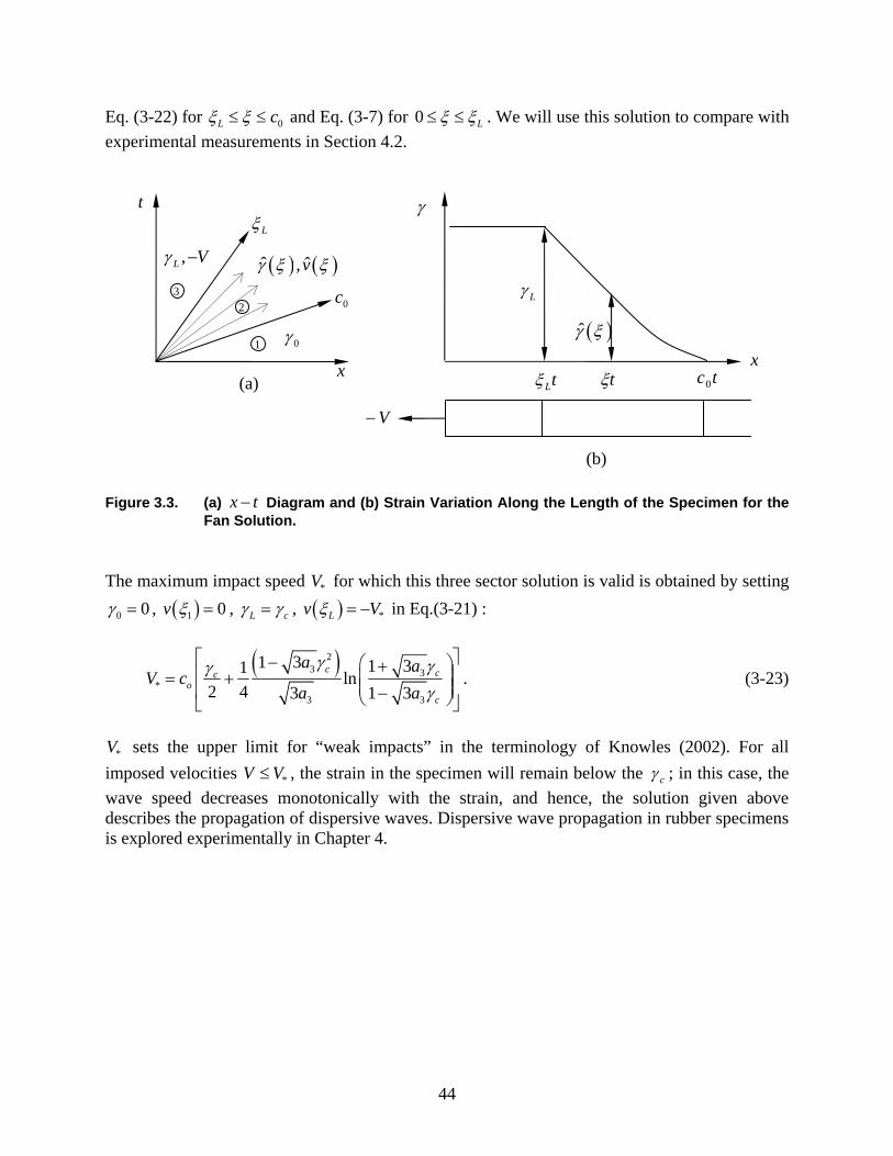
44

Eq. (3-22) for 0L cξ ξ≤ ≤ and Eq. (3-7) for 0 Lξ ξ≤ ≤ . We will use this solution to compare with experimental measurements in Section 4.2.

Figure 3.3. (a) x t− Diagram and (b) Strain Variation Along the Length of the Specimen for the

Fan Solution. The maximum impact speed *V for which this three sector solution is valid is obtained by setting

0 0γ = , ( )1 0v ξ = , L cγ γ= , ( ) *Lv Vξ = − in Eq.(3-21) :

( )23 3

*3 3

1 3 1 31 ln2 4 3 1 3

c cco

c

a aV c

a a

γ γγγ

⎡ ⎤− ⎛ ⎞+⎢ ⎥= + ⎜ ⎟⎜ ⎟⎢ ⎥−⎝ ⎠⎣ ⎦. (3-23)

*V sets the upper limit for “weak impacts” in the terminology of Knowles (2002). For all imposed velocities *V V≤ , the strain in the specimen will remain below the cγ ; in this case, the wave speed decreases monotonically with the strain, and hence, the solution given above describes the propagation of dispersive waves. Dispersive wave propagation in rubber specimens is explored experimentally in Chapter 4.

t

0c

Lξ

0γ

,L Vγ − ( ) ( )ˆ ˆ,vγ ξ ξ

x

V−

Lγ

( )γ̂ ξ

tc0tξLtξx

γ

(a)

(b)

1

2 3

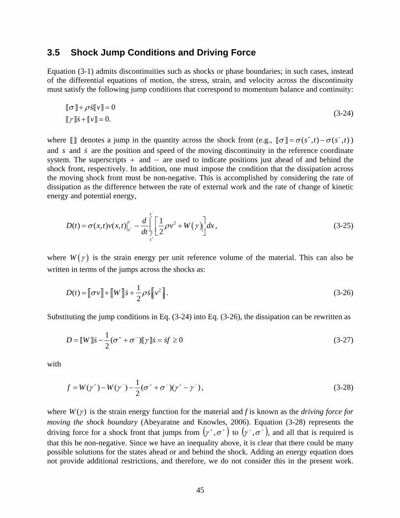
45

3.5 Shock Jump Conditions and Driving Force Equation (3-1) admits discontinuities such as shocks or phase boundaries; in such cases, instead of the differential equations of motion, the stress, strain, and velocity across the discontinuity must satisfy the following jump conditions that correspond to momentum balance and continuity:

00.

s vs v

σ ργ

+ =+ =

(3-24)

where denotes a jump in the quantity across the shock front (e.g., ( , ) ( , )s t s tσ σ σ+ −= − ) and s and s are the position and speed of the moving discontinuity in the reference coordinate system. The superscripts + and − are used to indicate positions just ahead of and behind the shock front, respectively. In addition, one must impose the condition that the dissipation across the moving shock front must be non-negative. This is accomplished by considering the rate of dissipation as the difference between the rate of external work and the rate of change of kinetic energy and potential energy,

( )21( ) ( , ) ( , )2

s

s

s

s

dD t x t v x t v W dxdt

σ ρ γ

−

−

+

+

⌠⎮⎮⌡

⎡ ⎤= − +⎢ ⎥⎣ ⎦, (3-25)

where ( )W γ is the strain energy per unit reference volume of the material. This can also be written in terms of the jumps across the shocks as:

21( )2

D t v W s s vσ ρ= + + . (3-26)

Substituting the jump conditions in Eq. (3-24) into Eq. (3-26), the dissipation can be rewritten as

1 ( ) 02

D W s s sfσ σ γ+ −= − + = ≥ (3-27)

with

1( ) ( ) ( )( )2

f W Wγ γ σ σ γ γ+ − + − + −= − − + − , (3-28)

where ( )W γ is the strain energy function for the material and f is known as the driving force for moving the shock boundary (Abeyaratne and Knowles, 2006). Equation (3-28) represents the driving force for a shock front that jumps from ( )++ σγ , to ( )−− σγ , , and all that is required is that this be non-negative. Since we have an inequality above, it is clear that there could be many possible solutions for the states ahead or and behind the shock. Adding an energy equation does not provide additional restrictions, and therefore, we do not consider this in the present work.

46

However, it must be noted that there is a coupling between the mechanical work and heat generation in the specimen that needs further investigation. 3.6 Shocks in a Cubic Material Although the cubic material model may not be applicable to high strain-rate problems (as we show in Chapter 4), it is convenient to examine shock solutions for this idealized model because of the possibility of obtaining simple analytical solutions. This model also allows a simple discussion of possible dissipation rules to be considered. After discussing possible shock states, we will consider the effect of the instantaneous elastic (dynamic) response observed at high strain-rates on shock formation. Consider a semi-infinite strip specimen that is at an initial state ( )0 0,vγ , with an imposed velocity (0, )v t V= − ; for the cubic material model, when *V V> , the imposed strain exceeds the strain at the inflection point and hence a shock is expected to form since larger strain levels move through the specimen with a greater speed than smaller strain levels. However, for what Knowles (2002, 2003) refers to as “intermediate impacts” one still expects the dispersive fan solution discussed in Section 3.4 to be appropriate until some critical stage is reached. Therefore, the problem is to find the end of the fan solution of Section 3.4, the jump across the shock, and the speed of the shock propagating through the specimen. Knowles (2002) goes through a complete analysis of this problem; here we summarize the main points of the analysis to motivate the experiments to be described in Section 5.1. The solution is formed in four sectors: a state corresponding to the initial conditions (sector 1), followed by a fan corresponding to dispersive waves (sector 2), followed by one or two constant sectors (sectors 3 and 4) that contain the shock; this is written formally as:

0 0

0

0ˆ ˆ( ) ( )

( , ) , ( , ) for

0

cv c

x t v x tv s

v V s

γ ξγ ξ ξ ξ ξ

γγ ξ ξγ ξ

+

+ + +

− −

>⎧ ⎧⎪ ⎪ ≤ ≤⎪ ⎪= =⎨ ⎨ < <⎪ ⎪⎪ ⎪ = − ≤ <⎩ ⎩

. (3-29)

For the fan sector, 0cξ ξ+ ≤ ≤ , ˆ( )γ ξ is given in Eq. (3-20) and ˆ( )v ξ is given in Eq. (3-21). The variation of strain with ξ is shown schematically in Figure 3.4. Now, ,γ γ+ − , and s are to be determined; but we only have the two shock jump relations in Eqs. (3-24). One may appeal to the dissipation inequality. The strain energy density corresponding to the cubic stress-strain relation in Eq. (2.6) is

4 3 2

3 2( )4 3 2

W E a aγ γ γγ⎛ ⎞

= + +⎜ ⎟⎝ ⎠

. (3-30)

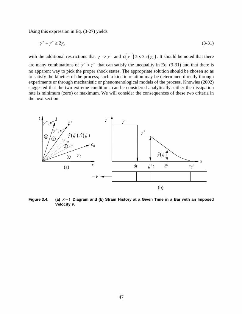
47

Using this expression in Eq. (3-27) yields

2 cγ γ γ+ −+ ≥ (3-31)

with the additional restrictions that γ γ− +> and ( ) ( )cc s cγ γ+ ≥ ≥ . It should be noted that there

are many combinations of γ γ− +> that can satisfy the inequality in Eq. (3-31) and that there is no apparent way to pick the proper shock states. The appropriate solution should be chosen so as to satisfy the kinetics of the process; such a kinetic relation may be determined directly through experiments or through mechanistic or phenomenological models of the process. Knowles (2002) suggested that the two extreme conditions can be considered analytically: either the dissipation rate is minimum (zero) or maximum. We will consider the consequences of these two criteria in the next section.

Figure 3.4. (a) x t− Diagram and (b) Strain History at a Given Time in a Bar with an Imposed

Velocity V.

t

0c

ξ +

0γ

,vγ + +

( ) ( )ˆ ˆ,vγ ξ ξ

x

,vγ − − s

V−

γ +

( )γ̂ ξ

tc0tξtξ +x

γ γ −

st(a)

(b)

1

2

3 4

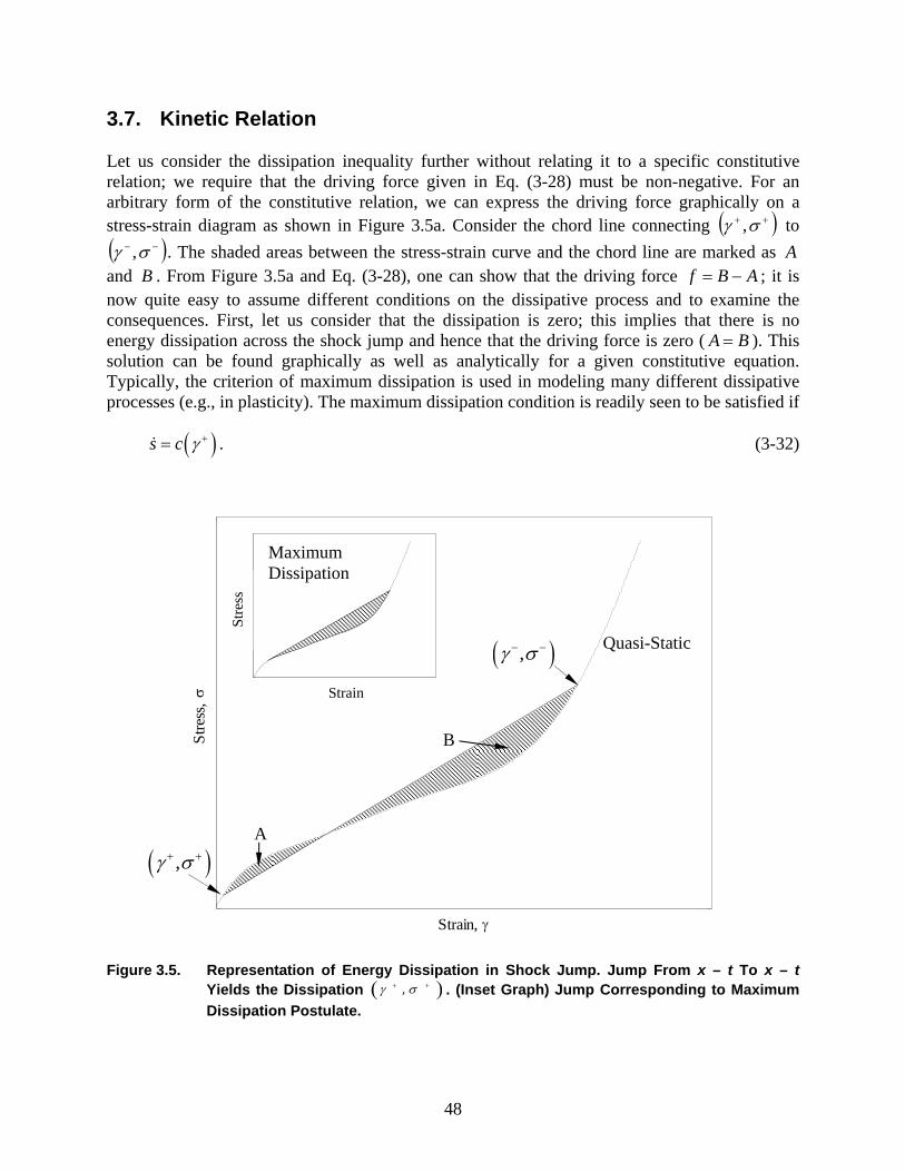
48

3.7. Kinetic Relation Let us consider the dissipation inequality further without relating it to a specific constitutive relation; we require that the driving force given in Eq. (3-28) must be non-negative. For an arbitrary form of the constitutive relation, we can express the driving force graphically on a stress-strain diagram as shown in Figure 3.5a. Consider the chord line connecting ( )++ σγ , to ( )−− σγ , . The shaded areas between the stress-strain curve and the chord line are marked as A and B . From Figure 3.5a and Eq. (3-28), one can show that the driving force f B A= − ; it is now quite easy to assume different conditions on the dissipative process and to examine the consequences. First, let us consider that the dissipation is zero; this implies that there is no energy dissipation across the shock jump and hence that the driving force is zero ( A B= ). This solution can be found graphically as well as analytically for a given constitutive equation. Typically, the criterion of maximum dissipation is used in modeling many different dissipative processes (e.g., in plasticity). The maximum dissipation condition is readily seen to be satisfied if

( )s c γ += . (3-32)

Figure 3.5. Representation of Energy Dissipation in Shock Jump. Jump From x – t To x – t

Yields the Dissipation ( ),γ σ+ + . (Inset Graph) Jump Corresponding to Maximum Dissipation Postulate.

( ),γ σ+ +

Strain, γ

Stre

ss, σ

A

B

( ),γ σ− −

Strain, γ

Stre

ss, σ

Strain

Stre

ss

Quasi-Static

Maximum Dissipation

49

This implies that the chord line connecting the starting and ending states of the shock is tangent to the stress-strain curve at the state ahead of the shock; this is called the Rayleigh line in the shock physics literature. Clearly, ( )s c γ += is the shock speed for a jump from ( )++ σγ , to

( )−− σγ , since this makes 0A = and maximizes B ; this shock travels with the speed of elastic waves in the pre shock state (see Figure 3.5). We will examine shock waves through experiments in Chapter 5. 3.8. Analysis of Free-Retraction Experiment in Rubber The free-retraction experiment introduced by Mason (1963) is considered next. The expected response corresponding to a cubic material model is easily assembled in terms of fan and constant sectors. 3.8.1. Governing Equations and General Solutions We consider a strip of rubber of length L ; x is the reference coordinate; 0 x L≤ ≤ . This strip is subjected to a prestrain of 0 0( ,0) 1xγ γ λ= = − by pulling on both ends. At 0t = , the end 0x = is released by setting the holding force to zero; this generates an unloading wave propagating into the material in the x-direction. By limiting considerations to times before this release wave has propagated to x L= , we may consider this as a one-dimensional semi-infinite strip of rubber occupying 0 x≤ < ∞ . The equations governing the balance of linear momentum and kinematic compatibility were described in Eq. (3-1). The details of the problem formulation and solution methodology applied to tensile impact can be found in Sections 3.4 and 3.6. Here we address unloading of a prestretched strip where it should be borne in mind that all experimental observations are made in the laboratory frame; the length scale in this frame corresponds to 0λ times the referential length scale and the wave speed in this frame is ( )0cλ γ . However, since we place physical markers on the specimen, interpreting all measurements through the referential coordinate poses no problem. As indicated in Section 3.2, all solutions to this problem must scale as x tξ = , as long as attention is restricted to times before arrival of waves reflected from x L= . Hence, the x t− plane is divided into sectors; two kinds of sectors are possible—fan sectors and constant sectors—and the analysis presented in Section 3.2 applies to this problem as well. Motivated by the experiments described later in this report, we take the strain and velocity in the specimen to be of the form

( ) ( )0 0

0ˆ,c

x t c ss

γ ξγ γ ξ ξ

γ ξ−

≥⎧⎪= ≥ >⎨⎪ <⎩

, ( ) ( )0

0

0ˆ,

cv x t v c s

v s

ξξ ξ

ξ−

≥⎧⎪= ≥ >⎨⎪ <⎩

. (3-33)

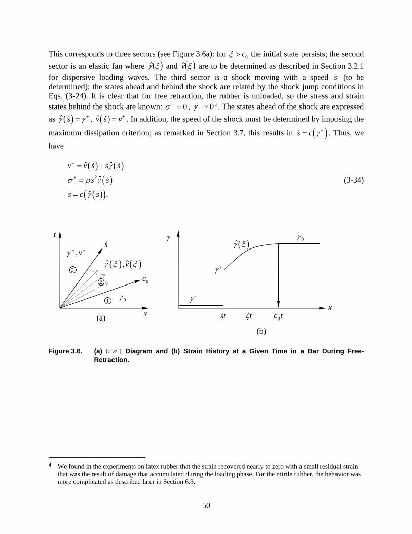
50

This corresponds to three sectors (see Figure 3.6a): for 0cξ > the initial state persists; the second sector is an elastic fan where ( )ξγ̂ and ( )ξv̂ are to be determined as described in Section 3.2.1 for dispersive loading waves. The third sector is a shock moving with a speed s (to be determined); the states ahead and behind the shock are related by the shock jump conditions in Eqs. (3-24). It is clear that for free retraction, the rubber is unloaded, so the stress and strain states behind the shock are known: 0σ − = , ~ 0γ − 4. The states ahead of the shock are expressed as ( )ˆ sγ γ += , ( )v̂ s v+= . In addition, the speed of the shock must be determined by imposing the

maximum dissipation criterion; as remarked in Section 3.7, this results in ( )s c γ += . Thus, we have

( ) ( )( )

( )( )

2

ˆˆ

ˆ

ˆ .

v v s s s

s s

s c s

γ

σ ρ γ

γ

−

+

= +

=

=

(3-34)

Figure 3.6. (a) ( ),γ σ− − Diagram and (b) Strain History at a Given Time in a Bar During Free-

Retraction.

4 We found in the experiments on latex rubber that the strain recovered nearly to zero with a small residual strain

that was the result of damage that accumulated during the loading phase. For the nitrile rubber, the behavior was more complicated as described later in Section 6.3.

t

0c

0γ

( ) ( )ˆ ˆ,vγ ξ ξ

x

,vγ − −s

(a)

1

2

3 γ +

( )γ̂ ξ

tc0tξx

γ

γ −

st

(b)

0γ

51

These equations are to be solved to determine v− , σ + , and s . Once the shock states are obtained, the displacement at any point can be calculated by integrating the particle velocity; the displacement in the different sectors can be written as:

( )

( )

2

2

ˆ( , ) for

ˆ .

o

o

o o

o oc

s

oc

x c

u x t x x v d c s

vx x v d x v t ss

ξ

γ ξ

γ ζ ζ ζ ξ

γ ζ ζ ζ ξ

−

−− −

⎧⎪ ≥⎪⎪⎪⎪= − ≥ ≥⎨⎪⎪⎛ ⎞⎪ − − + >⎜ ⎟⎪⎜ ⎟⎪⎝ ⎠⎩

∫

∫

(3-35)

The particle trajectory given by ( , ) ( , )y x t x u x t= + is then obtained by numerical integration. The details of the strain and particle velocity variation with position and time, of course, depend on the particular stress-strain curve that is assumed for the material. In the following subsection, we will describe the unloading solutions provided by the cubic material model (although we show in Chapter 6 that this may not be representative of the material behavior under the dynamic conditions of unloading). 3.8.2. Unloading Waves in Cubic Material Model For the cubic material model, the solution for the strain, particle velocity, and displacement in the fan sector are given in Eqs. (3-20) to (3-22) with the positive sign considered in Eq. (3-20) since the strain is expected to be larger than cγ :

( ) 2 20

0 3

1ˆ for3c c cc c c

c aγ ξ γ ξ ξ= + − ≤ ≤ . (3-36)

Then the particle velocity at any point in the fan sector can be found by integrating from the beginning of the fan sector at 0cξ = :

2 22 2 2 2 2

0 0 2 20 3 0 0

1ˆ( ) ln2 3

cc c c

c

cv c c c c c

c a c c c

ξ ξξ ξ ξ

⎡ ⎤⎛ ⎞+ −⎢ ⎥⎜ ⎟= − − − −⎜ ⎟⎢ ⎥+ −⎝ ⎠⎣ ⎦

. (3-37)

Note that a shock must form at some strain level cγ γ> because the wave speeds increase for

cγ γ< . The procedure discussed above can be used for numerical estimates of the particle trajectory. Free-retraction experiments are discussed in Chapter 6.

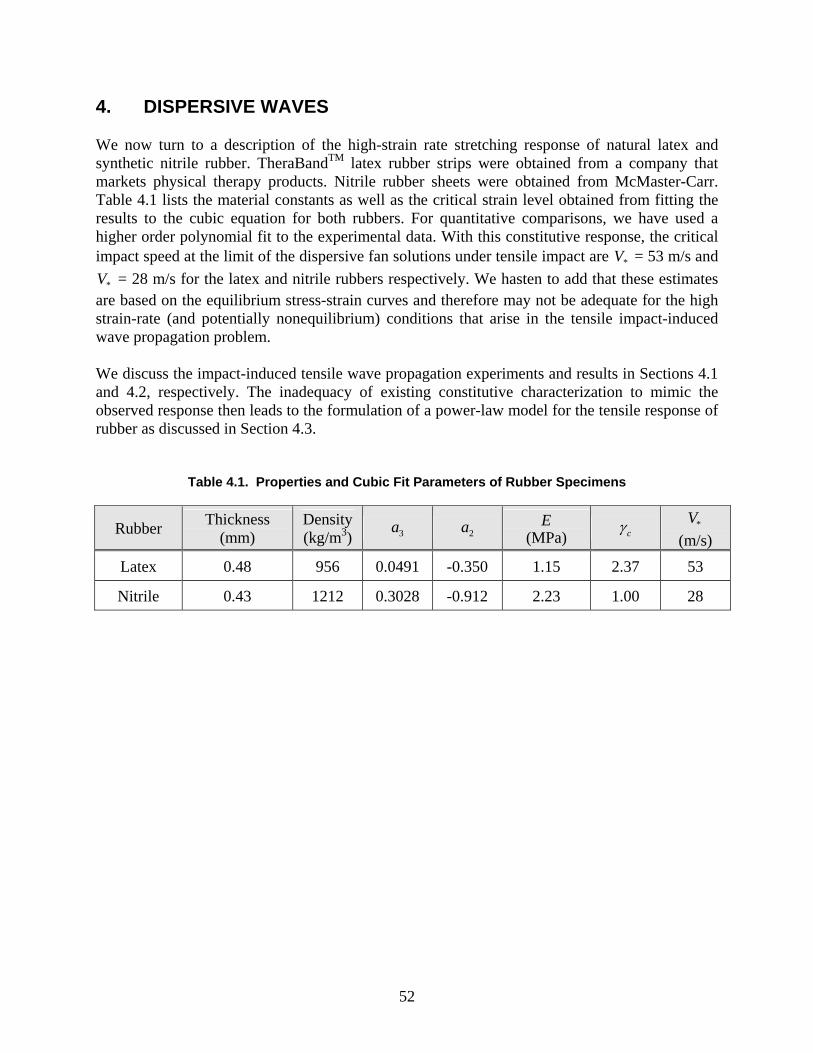
52

4. DISPERSIVE WAVES We now turn to a description of the high-strain rate stretching response of natural latex and synthetic nitrile rubber. TheraBandTM latex rubber strips were obtained from a company that markets physical therapy products. Nitrile rubber sheets were obtained from McMaster-Carr. Table 4.1 lists the material constants as well as the critical strain level obtained from fitting the results to the cubic equation for both rubbers. For quantitative comparisons, we have used a higher order polynomial fit to the experimental data. With this constitutive response, the critical impact speed at the limit of the dispersive fan solutions under tensile impact are *V = 53 m/s and

*V = 28 m/s for the latex and nitrile rubbers respectively. We hasten to add that these estimates are based on the equilibrium stress-strain curves and therefore may not be adequate for the high strain-rate (and potentially nonequilibrium) conditions that arise in the tensile impact-induced wave propagation problem. We discuss the impact-induced tensile wave propagation experiments and results in Sections 4.1 and 4.2, respectively. The inadequacy of existing constitutive characterization to mimic the observed response then leads to the formulation of a power-law model for the tensile response of rubber as discussed in Section 4.3.

Table 4.1. Properties and Cubic Fit Parameters of Rubber Specimens

Rubber Thickness (mm)

Density (kg/m3) 3a 2a E

(MPa) cγ *V (m/s)

Latex 0.48 956 0.0491 -0.350 1.15 2.37 53

Nitrile 0.43 1212 0.3028 -0.912 2.23 1.00 28

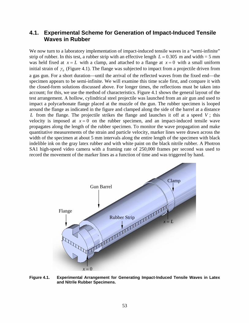
53

4.1. Experimental Scheme for Generation of Impact-Induced Tensile Waves in Rubber

We now turn to a laboratory implementation of impact-induced tensile waves in a “semi-infinite” strip of rubber. In this test, a rubber strip with an effective length 0.305L = m and width = 5 mm was held fixed at Lx = with a clamp, and attached to a flange at 0x = with a small uniform initial strain of 0γ (Figure 4.1). The flange was subjected to impact from a projectile driven from a gas gun. For a short duration—until the arrival of the reflected waves from the fixed end—the specimen appears to be semi-infinite. We will examine this time scale first, and compare it with the closed-form solutions discussed above. For longer times, the reflections must be taken into account; for this, we use the method of characteristics. Figure 4.1 shows the general layout of the test arrangement. A hollow, cylindrical steel projectile was launched from an air gun and used to impact a polycarbonate flange placed at the muzzle of the gun. The rubber specimen is looped around the flange as indicated in the figure and clamped along the side of the barrel at a distance L from the flange. The projectile strikes the flange and launches it off at a speed V ; this velocity is imposed at 0=x on the rubber specimen, and an impact-induced tensile wave propagates along the length of the rubber specimen. To monitor the wave propagation and make quantitative measurements of the strain and particle velocity, marker lines were drawn across the width of the specimen at about 5 mm intervals along the entire length of the specimen with black indelible ink on the gray latex rubber and with white paint on the black nitrile rubber. A Photron SA1 high-speed video camera with a framing rate of 250,000 frames per second was used to record the movement of the marker lines as a function of time and was triggered by hand.

Figure 4.1. Experimental Arrangement for Generating Impact-Induced Tensile Waves in Latex

and Nitrile Rubber Specimens.

Flange

Gun Barrel

Rubber Strip

Clamp

0x =

x L=

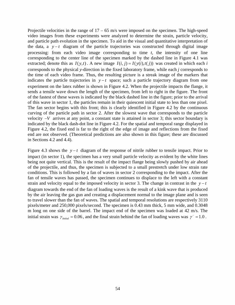
54

Projectile velocities in the range of 17 – 65 m/s were imposed on the specimen. The high-speed video images from these experiments were analyzed to determine the strain, particle velocity, and particle path evolution in the specimen. To aid in the visual and quantitative interpretation of the data, a y t− diagram of the particle trajectories was constructed through digital image processing: from each video image corresponding to time t, the intensity of one line corresponding to the center line of the specimen marked by the dashed line in Figure 4.1 was extracted; denote this as ( , )I y t . A new image ( , ) ( ( ), ( ))I i j I y i t j= was created in which each i corresponds to the physical y-direction in the fixed laboratory frame, while each j corresponds to the time of each video frame. Thus, the resulting picture is a streak image of the markers that indicates the particle trajectories in y t− space; such a particle trajectory diagram from one experiment on the latex rubber is shown in Figure 4.2. When the projectile impacts the flange, it sends a tensile wave down the length of the specimen, from left to right in the figure. The front of the fastest of these waves is indicated by the black dashed line in the figure; prior to the arrival of this wave in sector 1, the particles remain in their quiescent initial state to less than one pixel. The fan sector begins with this front; this is clearly identified in Figure 4.2 by the continuous curving of the particle path in sector 2. After the slowest wave that corresponds to the particle velocity V− arrives at any point, a constant state is attained in sector 3; this sector boundary is indicated by the black dash-dot line in Figure 4.2. For the spatial and temporal range displayed in Figure 4.2, the fixed end is far to the right of the edge of image and reflections from the fixed end are not observed. (Theoretical predictions are also shown in this figure; these are discussed in Sections 4.2 and 4.4). Figure 4.3 shows the y t− diagram of the response of nitrile rubber to tensile impact. Prior to impact (in sector 1), the specimen has a very small particle velocity as evident by the white lines being not quite vertical. This is the result of the impact flange being slowly pushed by air ahead of the projectile, and thus, the specimen is subjected to a small prestretch under low strain rate conditions. This is followed by a fan of waves in sector 2 corresponding to the impact. After the fan of tensile waves has passed, the specimen continues to displace to the left with a constant strain and velocity equal to the imposed velocity in sector 3. The change in contrast in the y t− diagram towards the end of the fan of loading waves is the result of a kink wave that is produced by the air leaving the gas gun and creating a displacement normal to the image plane and is seen to travel slower than the fan of waves. The spatial and temporal resolutions are respectively 3110 pixels/meter and 250,000 pixels/second. The specimen is 0.43 mm thick, 5 mm wide, and 0.3048 m long on one side of the barrel. The impact end of the specimen was loaded at 42 m/s. The initial strain was 0.06Initialγ = , and the final strain behind the fan of loading waves was 1.0γ − = .

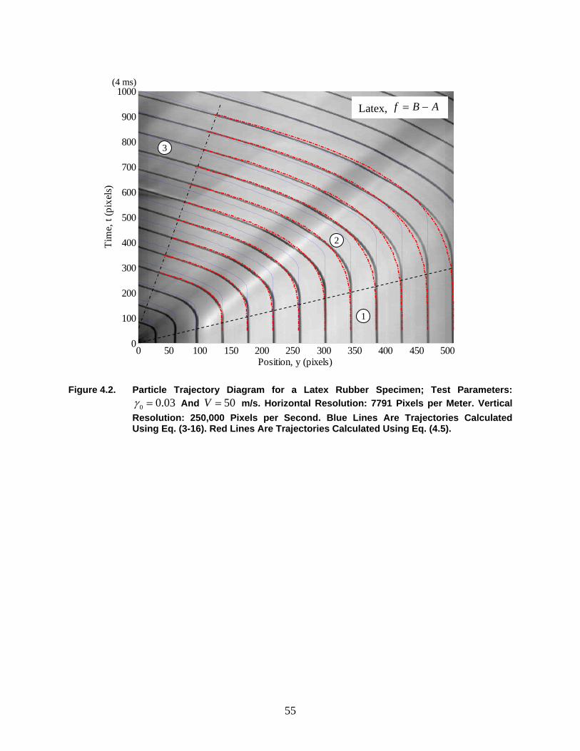
55

Figure 4.2. Particle Trajectory Diagram for a Latex Rubber Specimen; Test Parameters:

0 0.03γ = And 50V = m/s. Horizontal Resolution: 7791 Pixels per Meter. Vertical Resolution: 250,000 Pixels per Second. Blue Lines Are Trajectories Calculated Using Eq. (3-16). Red Lines Are Trajectories Calculated Using Eq. (4.5).

(0.064 m) 0 50 100 150 200 250 300 350 400 450 5000

100

200

300

400

500

600

700

800

900

1000

Position, y (pixels)

Tim

e, t

(pix

els)

(4 ms)

Latex, f B A= −

1

2

3

56

Figure 4.3. Particle Trajectory Diagram for a Nitrile Rubber Specimen; Test Parameters: 0 0.06γ = and 42V = m/s. Horizontal Resolution: 3110 Pixels Per Meter. Vertical

Resolution: 250,000 Pixels Per Second. Red Lines Are Trajectories Calculated Using Eq. (4.5).

4.2. Comparison of Measured and Calculated Particle Trajectories We are now ready to compare these experimental results to the theory described in Section 3.4, based on the cubic model of the constitutive behavior. The particle trajectory for the latex rubber was calculated using Eq. (3-16). The blue lines in Figure 4.2 compare the calculated particle trajectories with the experimental measurement. While the general trends of the predicted trajectories correspond qualitatively to the experimental observations—that there is a fan solution—a quantitative match is clearly not observed. The discrepancy is the largest in the early stages of the wave propagation: the fastest wave observed in the experiment is significantly faster than that predicted using the quasi-static stress-strain curve. Furthermore, based on the quasi-static characterization, the maximum impact speed that can be sustained without exceeding the critical strain is *V = 53 m/s; in the experiments, we exceeded this by a factor of 1.2, but continued to observe dispersive wave propagation, without discontinuities or shocks. Similar discrepancies were observed for the nitrile rubber; the particle trajectories in Figure 4.3 could not be matched by using the quasi-static stress-strain response. Also, the critical speed of

*V = 28 m/s was exceeded by a factor of nearly 2.3, and still only dispersive waves were

0 50 100 150 200 250 300 350 4000

200

400

600

800

1000

1200

1400

1600

1800

Position, y (pixels)

Tim

e, t

(pix

els)

(0.129 m)

(7.2 ms) Nitrile, 24 oT C=

Power-Law

1

2

3

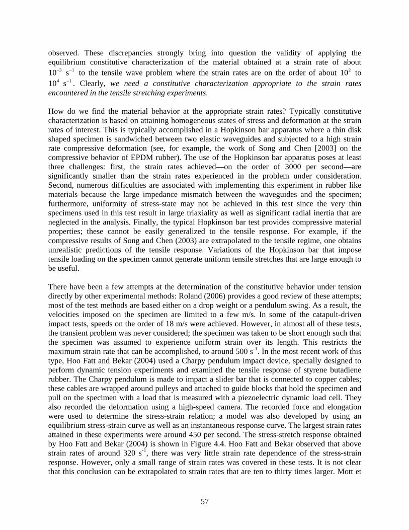
57

observed. These discrepancies strongly bring into question the validity of applying the equilibrium constitutive characterization of the material obtained at a strain rate of about

310− 1s− to the tensile wave problem where the strain rates are on the order of about 210 to 410 1s− . Clearly, we need a constitutive characterization appropriate to the strain rates

encountered in the tensile stretching experiments. How do we find the material behavior at the appropriate strain rates? Typically constitutive characterization is based on attaining homogeneous states of stress and deformation at the strain rates of interest. This is typically accomplished in a Hopkinson bar apparatus where a thin disk shaped specimen is sandwiched between two elastic waveguides and subjected to a high strain rate compressive deformation (see, for example, the work of Song and Chen [2003] on the compressive behavior of EPDM rubber). The use of the Hopkinson bar apparatus poses at least three challenges: first, the strain rates achieved—on the order of 3000 per second—are significantly smaller than the strain rates experienced in the problem under consideration. Second, numerous difficulties are associated with implementing this experiment in rubber like materials because the large impedance mismatch between the waveguides and the specimen; furthermore, uniformity of stress-state may not be achieved in this test since the very thin specimens used in this test result in large triaxiality as well as significant radial inertia that are neglected in the analysis. Finally, the typical Hopkinson bar test provides compressive material properties; these cannot be easily generalized to the tensile response. For example, if the compressive results of Song and Chen (2003) are extrapolated to the tensile regime, one obtains unrealistic predictions of the tensile response. Variations of the Hopkinson bar that impose tensile loading on the specimen cannot generate uniform tensile stretches that are large enough to be useful. There have been a few attempts at the determination of the constitutive behavior under tension directly by other experimental methods: Roland (2006) provides a good review of these attempts; most of the test methods are based either on a drop weight or a pendulum swing. As a result, the velocities imposed on the specimen are limited to a few m/s. In some of the catapult-driven impact tests, speeds on the order of 18 m/s were achieved. However, in almost all of these tests, the transient problem was never considered; the specimen was taken to be short enough such that the specimen was assumed to experience uniform strain over its length. This restricts the maximum strain rate that can be accomplished, to around 500 s-1. In the most recent work of this type, Hoo Fatt and Bekar (2004) used a Charpy pendulum impact device, specially designed to perform dynamic tension experiments and examined the tensile response of styrene butadiene rubber. The Charpy pendulum is made to impact a slider bar that is connected to copper cables; these cables are wrapped around pulleys and attached to guide blocks that hold the specimen and pull on the specimen with a load that is measured with a piezoelectric dynamic load cell. They also recorded the deformation using a high-speed camera. The recorded force and elongation were used to determine the stress-strain relation; a model was also developed by using an equilibrium stress-strain curve as well as an instantaneous response curve. The largest strain rates attained in these experiments were around 450 per second. The stress-stretch response obtained by Hoo Fatt and Bekar (2004) is shown in Figure 4.4. Hoo Fatt and Bekar observed that above strain rates of around 320 s-1, there was very little strain rate dependence of the stress-strain response. However, only a small range of strain rates was covered in these tests. It is not clear that this conclusion can be extrapolated to strain rates that are ten to thirty times larger. Mott et

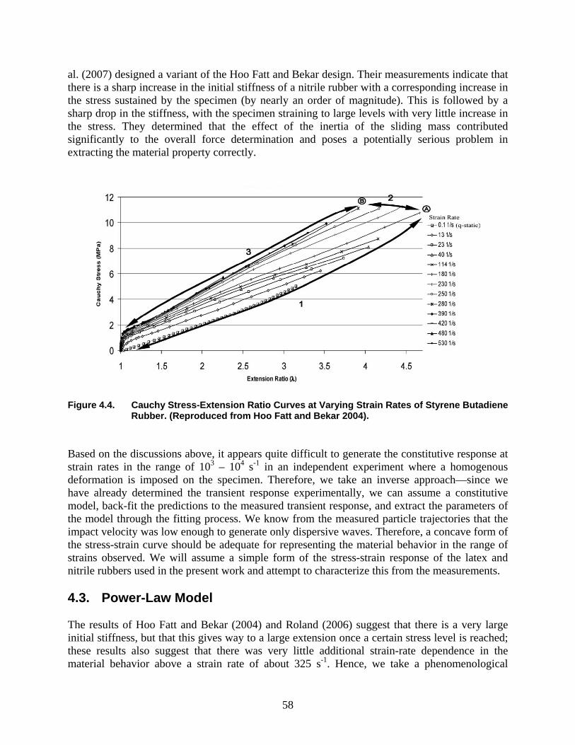
58

al. (2007) designed a variant of the Hoo Fatt and Bekar design. Their measurements indicate that there is a sharp increase in the initial stiffness of a nitrile rubber with a corresponding increase in the stress sustained by the specimen (by nearly an order of magnitude). This is followed by a sharp drop in the stiffness, with the specimen straining to large levels with very little increase in the stress. They determined that the effect of the inertia of the sliding mass contributed significantly to the overall force determination and poses a potentially serious problem in extracting the material property correctly.

Figure 4.4. Cauchy Stress-Extension Ratio Curves at Varying Strain Rates of Styrene Butadiene

Rubber. (Reproduced from Hoo Fatt and Bekar 2004). Based on the discussions above, it appears quite difficult to generate the constitutive response at strain rates in the range of 103 – 104 s-1 in an independent experiment where a homogenous deformation is imposed on the specimen. Therefore, we take an inverse approach—since we have already determined the transient response experimentally, we can assume a constitutive model, back-fit the predictions to the measured transient response, and extract the parameters of the model through the fitting process. We know from the measured particle trajectories that the impact velocity was low enough to generate only dispersive waves. Therefore, a concave form of the stress-strain curve should be adequate for representing the material behavior in the range of strains observed. We will assume a simple form of the stress-strain response of the latex and nitrile rubbers used in the present work and attempt to characterize this from the measurements. 4.3. Power-Law Model The results of Hoo Fatt and Bekar (2004) and Roland (2006) suggest that there is a very large initial stiffness, but that this gives way to a large extension once a certain stress level is reached; these results also suggest that there was very little additional strain-rate dependence in the material behavior above a strain rate of about 325 s-1. Hence, we take a phenomenological

59

approach and postulate the simplest possible stress-strain response for a strain-rate independent material that could produce dispersive waves of the kind observed in Figures 4.2 and 4.3. At this stage, we do not attempt to motivate this form of the constitutive behavior from micromechanics of deformation of the polymer chains. We use a model that allows for the possibility of extremely fast initial wave speeds: a power-law model of the following form appears to be adequate.

( )0 0nσ σ µ γ γ= + − , (4-1)

where 0σ is the stress at the initial strain 0γ (and determined from the equilibrium stress-strain curve), µ is the reference stress and n is the “hardening” parameter; in order to generate dispersive waves, the only restriction required in this model is that 0 1n< < . Figures 4.5 and 4.6 show the power-law model for a semi-infinite specimen corresponding to

0 0.03γ = , 1.0µ = MPa, and 0.5n = for latex and 0 0.06γ = , 2.1µ = MPa, and 0.47n = for nitrile. The quasi-static stress-strain curves are also shown for comparison. Two main differences arise in the stress-strain curves. First, the initial stiffness of the power-law model is quite high, but it quickly begins to drop and the stress begins to level out. Second, the inflection point seen in the quasi-static curves is not observed in the power-law model; therefore, the power-law model is not suitable for capturing shock formulation. Because we limit our consideration in this chapter to dispersive waves, this does not pose a problem. and show below that this power-law model is fully capable of capturing the propagation of dispersive waves.

4.4. Dispersive Waves in the Power-Law Material The wave speeds for this power-law model are then calculated as

( ) ( )1

2 12

01 nd nc

dσ µγ γ γ

ρ γ ρ

−⎛ ⎞= = −⎜ ⎟

⎝ ⎠. (4-2)

Note that as 0γ γ→ , c → ∞ ; there is no limit to the wave speed at small strains. Nevertheless, this does not pose any serious problems in calculating the particle trajectories, and if necessary, the problem can be fixed with a small initial segment with a finite wave speed. For this material model, consider the fan solution; using Eq. (4-2) in first of Eq. (3-3), we get the strain as a function of ξ , ( /x tξ = ):

121

10

nnnµγ γ ξ

ρ

−−⎛ ⎞

− = ⎜ ⎟⎝ ⎠

. (4-3)

60

Note that ( )1 0γ ξ γ→ as 1ξ → ∞ , the fastest characteristic. The particle velocity in the fan sector

is given by Eq. (3-4). Substituting for ( )c γ from Eqs. (4-2), we get an explicit expression for the particle velocity:

( )1

1112ˆ

1

nnnnv

nµξ ξρ

+−−⎛ ⎞⎛ ⎞= − ⎜ ⎟⎜ ⎟+⎝ ⎠⎝ ⎠

, (4-4)

where the initial condition is taken to be quiescent. Note that 1 01

nn

+<

− whenever 1n < ;

therefore, as 1ξ → ∞ , ˆ 0v → . The particle displacement is obtained by integrating Eq. (4-4); noting that ( )1 , ou t t xξ γ→ as 1ξ → ∞ , we get

( )1

1 211 11,

1

nnn n

on nu x t x x tn

µγρ

+− −− −⎛ ⎞−

= + ⎜ ⎟+ ⎝ ⎠. (4-5)

This expression can be evaluated, if the material constants µ and n as well as the initial strain

0γ are known. To apply the power-law model to the experimental measurements of the impact-induced tensile response, we adopt a simple strategy: obtain values of µ and n such that the experimentally determined particle trajectories in Figures 4.2 and 4.3 (and other similar measurements at different imposed speeds) are matched by the predictions in Eq. (4-5). The red dashed lines in Figure 4.2 show the particle trajectories calculated with the power-law model for the latex rubber, with 1µ = MPa and 0.5n = ; the red dashed lines in Figure 4.3 show the corresponding comparison for the particle trajectories for tensile impact of nitrile rubber, where the two parameters used were 2.1µ = MPa and 0.47n = . From these comparisons, it is clear that the calculated particle trajectories match the experimental results quite well quantitatively for both latex and nitrile rubber. There is a small deviation between the predictions and actual displacement for lines very far from the impact point, particularly for the nitrile rubber; this deviation is likely to be caused either by the very stiff response of the power-law model at small strain levels or by the strain-rate dependence in material response at the smaller strain rates experienced at these material points; we consider this in the next paragraph. One startling result of the comparison shown above is that one set of values of µ and n can be found for each material that provides a good estimate of the particle trajectories where the strain rates vary in the range of 500 – 104 s-1 at different positions in the specimen. The agreement between the predictions of a strain-rate independent constitutive model and the experiment suggests that the material exhibits very little strain rate sensitivity in this range. We will take this to be the instantaneous elastic response at high strain rates. The stress-strain curve calculated from the best-fit power-law model (red line) is compared to the quasi-static stress-strain curve (black line) in Figures 4.5 and 4.6 for the latex and nitrile rubbers, respectively. For strain rates

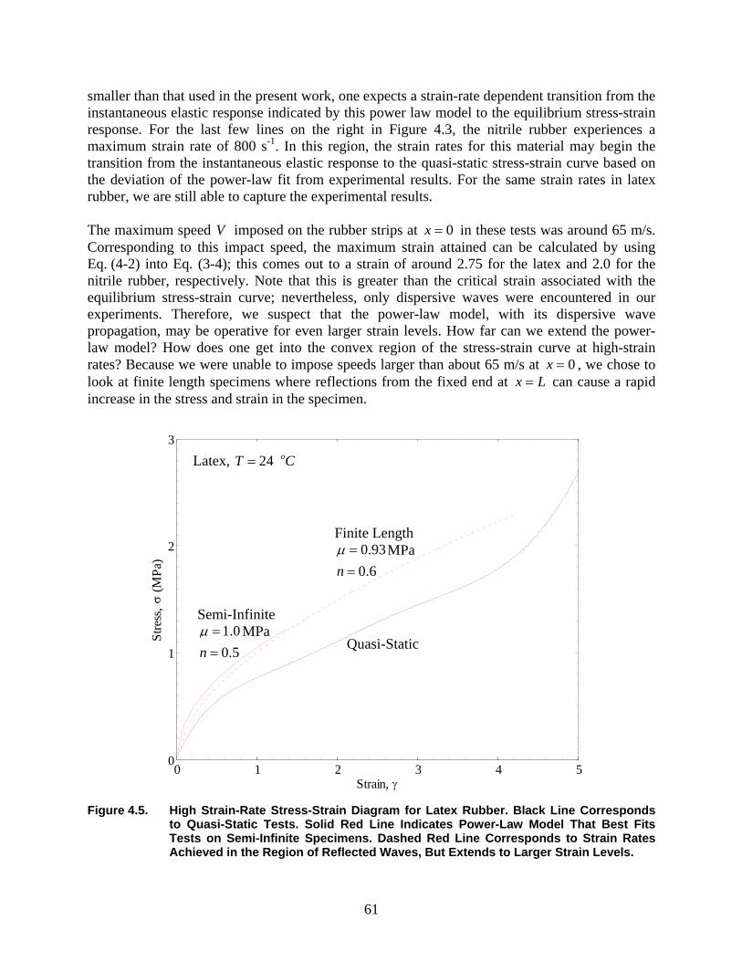
61

smaller than that used in the present work, one expects a strain-rate dependent transition from the instantaneous elastic response indicated by this power law model to the equilibrium stress-strain response. For the last few lines on the right in Figure 4.3, the nitrile rubber experiences a maximum strain rate of 800 s-1. In this region, the strain rates for this material may begin the transition from the instantaneous elastic response to the quasi-static stress-strain curve based on the deviation of the power-law fit from experimental results. For the same strain rates in latex rubber, we are still able to capture the experimental results. The maximum speed V imposed on the rubber strips at 0x = in these tests was around 65 m/s. Corresponding to this impact speed, the maximum strain attained can be calculated by using Eq. (4-2) into Eq. (3-4); this comes out to a strain of around 2.75 for the latex and 2.0 for the nitrile rubber, respectively. Note that this is greater than the critical strain associated with the equilibrium stress-strain curve; nevertheless, only dispersive waves were encountered in our experiments. Therefore, we suspect that the power-law model, with its dispersive wave propagation, may be operative for even larger strain levels. How far can we extend the power-law model? How does one get into the convex region of the stress-strain curve at high-strain rates? Because we were unable to impose speeds larger than about 65 m/s at 0x = , we chose to look at finite length specimens where reflections from the fixed end at x L= can cause a rapid increase in the stress and strain in the specimen.

Figure 4.5. High Strain-Rate Stress-Strain Diagram for Latex Rubber. Black Line Corresponds

to Quasi-Static Tests. Solid Red Line Indicates Power-Law Model That Best Fits Tests on Semi-Infinite Specimens. Dashed Red Line Corresponds to Strain Rates Achieved in the Region of Reflected Waves, But Extends to Larger Strain Levels.

0 1 2 3 4 50

1

2

3

Strain, γ

Stre

ss, σ

(MPa

)

Latex, 24 oT C=

Semi-Infinite 1.00.5n

µ ==

MPa

Finite Length 0.930.6n

µ ==

MPa

Quasi-Static

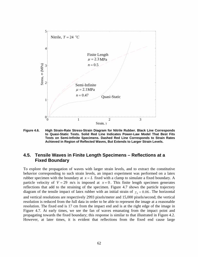
62

Figure 4.6. High Strain-Rate Stress-Strain Diagram for Nitrile Rubber. Black Line Corresponds

to Quasi-Static Tests. Solid Red Line Indicates Power-Law Model That Best Fits Tests on Semi-Infinite Specimens. Dashed Red Line Corresponds to Strain Rates Achieved in Region of Reflected Waves, But Extends to Larger Strain Levels.

4.5. Tensile Waves in Finite Length Specimens – Reflections at a

Fixed Boundary To explore the propagation of waves with larger strain levels, and to extract the constitutive behavior corresponding to such strain levels, an impact experiment was performed on a latex rubber specimen with the boundary at x L= fixed with a clamp to simulate a fixed boundary. A particle velocity of 29V = m/s is imposed at 0x = . This finite length specimen generates reflections that add to the straining of the specimen. Figure 4.7 shows the particle trajectory diagram of the tensile impact of latex rubber with an initial strain of 0 0.06γ = . The horizontal and vertical resolutions are respectively 2993 pixels/meter and 15,000 pixels/second; the vertical resolution is reduced from the full data in order to be able to represent the image at a reasonable resolution. The fixed end is 17 cm from the impact end and is at the right edge of the image in Figure 4.7. At early times, we see the fan of waves emanating from the impact point and propagating towards the fixed boundary; this response is similar to that illustrated in Figure 4.2. However, at later times, it is evident that reflections from the fixed end cause large

0 1 2 30

1

2

3

4

5

Strain, γ

Stre

ss, σ

(MPa

)

Semi-Infinite 2.10.47n

µ ==

MPa

Nitrile, 24 oT C=

Finite Length 2.30.5n

µ ==

MPa

Quasi-Static

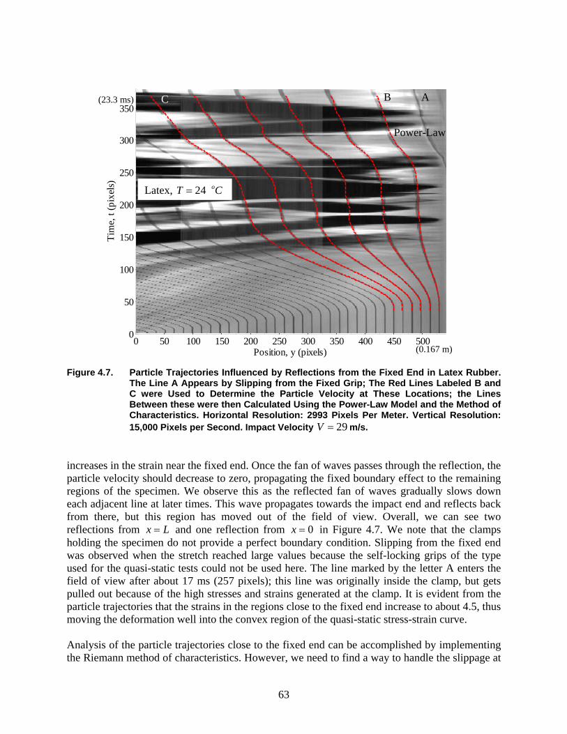
63

Figure 4.7. Particle Trajectories Influenced by Reflections from the Fixed End in Latex Rubber.

The Line A Appears by Slipping from the Fixed Grip; The Red Lines Labeled B and C were Used to Determine the Particle Velocity at These Locations; the Lines Between these were then Calculated Using the Power-Law Model and the Method of Characteristics. Horizontal Resolution: 2993 Pixels Per Meter. Vertical Resolution: 15,000 Pixels per Second. Impact Velocity 29V = m/s.

increases in the strain near the fixed end. Once the fan of waves passes through the reflection, the particle velocity should decrease to zero, propagating the fixed boundary effect to the remaining regions of the specimen. We observe this as the reflected fan of waves gradually slows down each adjacent line at later times. This wave propagates towards the impact end and reflects back from there, but this region has moved out of the field of view. Overall, we can see two reflections from x L= and one reflection from 0x = in Figure 4.7. We note that the clamps holding the specimen do not provide a perfect boundary condition. Slipping from the fixed end was observed when the stretch reached large values because the self-locking grips of the type used for the quasi-static tests could not be used here. The line marked by the letter A enters the field of view after about 17 ms (257 pixels); this line was originally inside the clamp, but gets pulled out because of the high stresses and strains generated at the clamp. It is evident from the particle trajectories that the strains in the regions close to the fixed end increase to about 4.5, thus moving the deformation well into the convex region of the quasi-static stress-strain curve. Analysis of the particle trajectories close to the fixed end can be accomplished by implementing the Riemann method of characteristics. However, we need to find a way to handle the slippage at

C

0 50 100 150 200 250 300 350 400 450 5000

50

100

150

200

250

300

350

Position, y (pixels)

Tim

e, t

(pix

els)

B A C

(0.167 m)

(23.3 ms)

Latex, 24 oT C=

Power-Law

64

the clamped end. We accomplished this by calculating the velocity of the line closest to fixed end (marked as B in Figure 4.7) as well as the first line to remain within the y t− diagram for t < 23 ms (marked as C in Figure 4.7) from the measured particle trajectory. Since these two lines correspond to material points, we now have the particle velocity prescribed at two material points for all times of interest; implementing the method of characteristics is then straightforward. This procedure avoids defining the slipping condition exactly when such slipping occurs as well as the fact that we do not have data points near the impact end at later times. The parameters for the power-law model, 0.93µ = MPa and 0.6n = , were obtained by matching the experimental particle trajectories near the point of impact, but prior to the arrival of reflected waves. These parameters were then used in the method of characteristics to calculate the particle path for points between the two lines B and C; the calculated particle trajectories match the observed paths quite well. The stress-strain path taken by the line B is displayed by the dashed red line in Figure 4.5; this is simply a continuation of the power-law model to strain levels of about 4.5. These material points have been strained well past the point of inflection and into the region where significant stiffening of the rubber occurs under quasi-static loading. To gain more confidence in this inverse process of extracting the stress-strain variation, a direct measurement of the force was performed. A piezoelectric force transducer (Model 208C01 from PCB Piezotronics, with a maximum force of 0.04448 kN and a frequency response of 36 kHz) was used to measure the force generated at the fixed end; the force measured at x L= is shown as a function of time by the black line in Figure 4.8. This force is also calculated from the solution obtained above using the method of characteristics; this is shown by the red dashed line in Figure 4.8. The agreement between the two is reasonably good considering that the actual force measurements are performed at a small distance away from the position where the calculations were performed. From these comparisons, we conclude that the power-law model of the stress-strain curve is a very good representation of the constitutive curve for impact-induced tensile wave propagation in rubber for strain levels up to 4.5 for latex rubber. The same procedure was used to extend the characterization of the dynamic response of the nitrile rubber. An impact experiment was performed with the boundary at x L= fixed with a clamp and particle velocity of 34V = m/s is imposed at 0x = . Figure 4.9 shows the particle trajectory diagram of the tensile impact of nitrile rubber with an initial strain of 0.06γ = . The horizontal and vertical resolutions are respectively 4194 pixels/meter and 15,000 pixels/second; the vertical resolution is reduced from the full data in order to be able to represent the image at a reasonable resolution. The fixed end is 16.5 cm from the impact end and is at the right edge of the image in Figure 4.9. As with the latex rubber, the particle trajectories prior to the arrival of the reflected waves were fitted using a power-law model, and these parameters were then used in the solution by the method of characteristics to calculate the particle trajectories between the lines marked A and B in Figure 4.9. The partially slipping boundary condition was handled in the same manner as described above. The agreement between the experiment and model is extremely good. The stress-strain path taken by the point corresponding to line A is shown in Figure 4.6 by the dashed line; it is simply a continuation of the power-law model to larger strain levels. It is

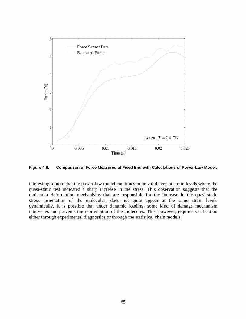
65

Figure 4.8. Comparison of Force Measured at Fixed End with Calculations of Power-Law Model. interesting to note that the power-law model continues to be valid even at strain levels where the quasi-static test indicated a sharp increase in the stress. This observation suggests that the molecular deformation mechanisms that are responsible for the increase in the quasi-static stress—orientation of the molecules—does not quite appear at the same strain levels dynamically. It is possible that under dynamic loading, some kind of damage mechanism intervenes and prevents the reorientation of the molecules. This, however, requires verification either through experimental diagnostics or through the statistical chain models.

0 0.005 0.01 0.015 0.02 0.0250

1

2

3

4

5

6

Time (s)

Forc

e (N

)

Force Sensor DataEstimated Force

Latex, 24 oT C=

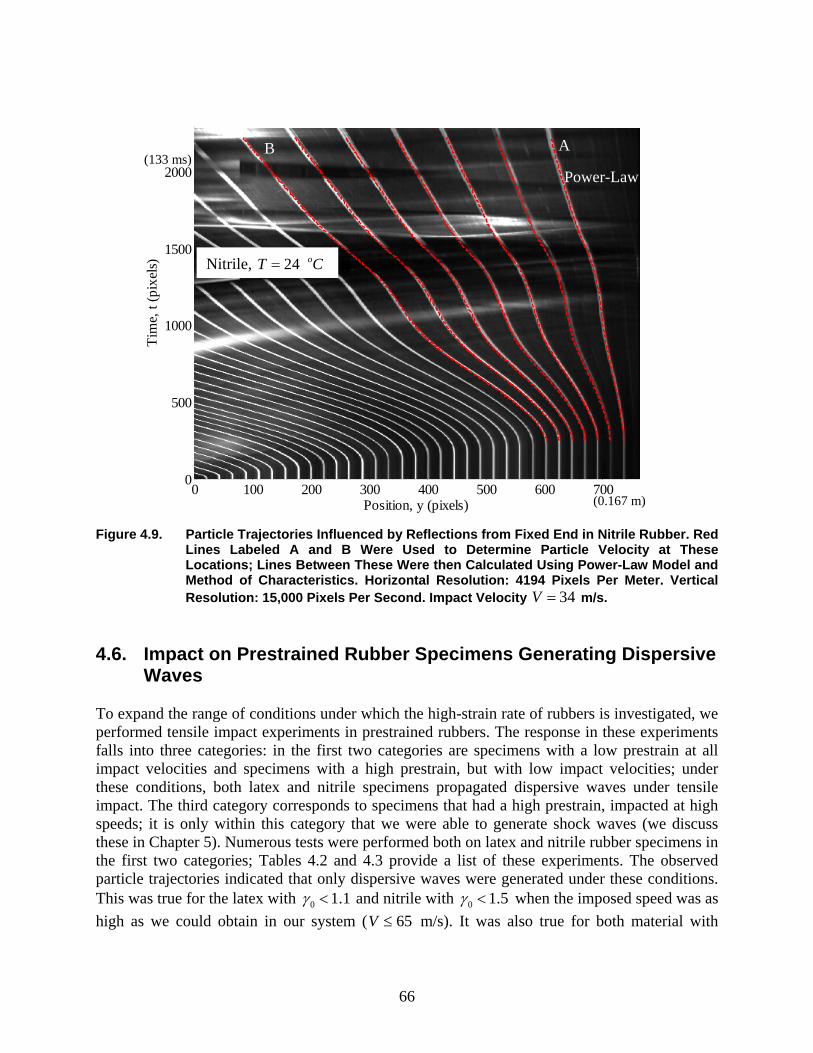
66

Figure 4.9. Particle Trajectories Influenced by Reflections from Fixed End in Nitrile Rubber. Red

Lines Labeled A and B Were Used to Determine Particle Velocity at These Locations; Lines Between These Were then Calculated Using Power-Law Model and Method of Characteristics. Horizontal Resolution: 4194 Pixels Per Meter. Vertical Resolution: 15,000 Pixels Per Second. Impact Velocity 34V = m/s.

4.6. Impact on Prestrained Rubber Specimens Generating Dispersive

Waves To expand the range of conditions under which the high-strain rate of rubbers is investigated, we performed tensile impact experiments in prestrained rubbers. The response in these experiments falls into three categories: in the first two categories are specimens with a low prestrain at all impact velocities and specimens with a high prestrain, but with low impact velocities; under these conditions, both latex and nitrile specimens propagated dispersive waves under tensile impact. The third category corresponds to specimens that had a high prestrain, impacted at high speeds; it is only within this category that we were able to generate shock waves (we discuss these in Chapter 5). Numerous tests were performed both on latex and nitrile rubber specimens in the first two categories; Tables 4.2 and 4.3 provide a list of these experiments. The observed particle trajectories indicated that only dispersive waves were generated under these conditions. This was true for the latex with 0 1.1γ < and nitrile with 0 1.5γ < when the imposed speed was as high as we could obtain in our system ( 65V ≤ m/s). It was also true for both material with

0 100 200 300 400 500 600 7000

500

1000

1500

2000

Position, y (pixels)

Tim

e, t

(pix

els)

B A

(0.167 m)

(133 ms)

Nitrile, 24 oT C=

Power-Law

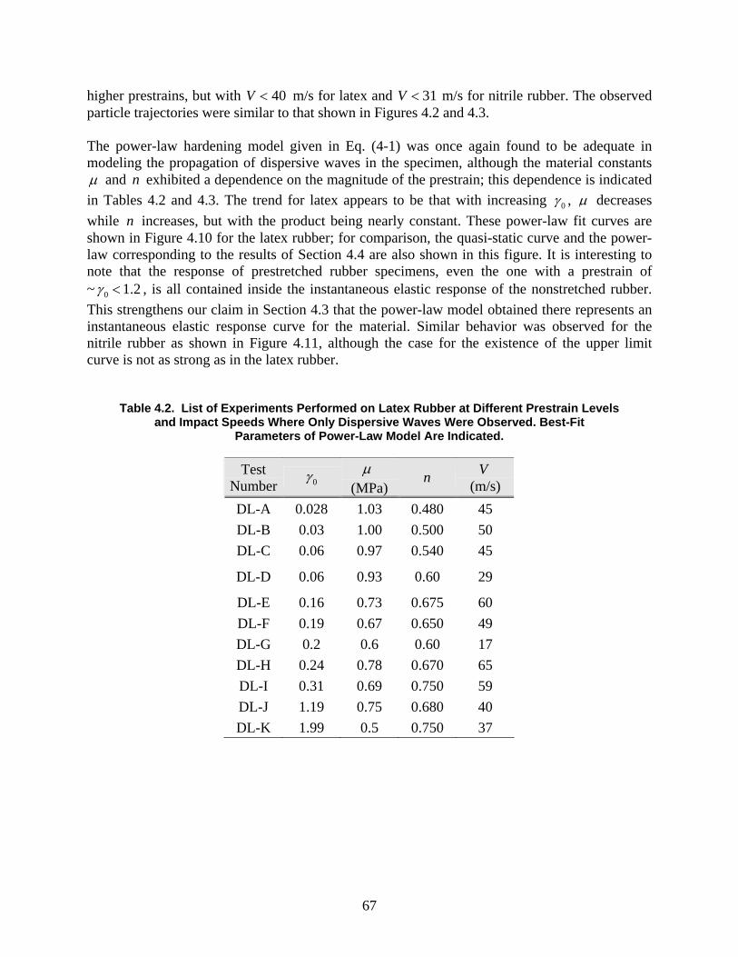
67

higher prestrains, but with 40V < m/s for latex and 31V < m/s for nitrile rubber. The observed particle trajectories were similar to that shown in Figures 4.2 and 4.3. The power-law hardening model given in Eq. (4-1) was once again found to be adequate in modeling the propagation of dispersive waves in the specimen, although the material constants µ and n exhibited a dependence on the magnitude of the prestrain; this dependence is indicated in Tables 4.2 and 4.3. The trend for latex appears to be that with increasing 0γ , µ decreases while n increases, but with the product being nearly constant. These power-law fit curves are shown in Figure 4.10 for the latex rubber; for comparison, the quasi-static curve and the power-law corresponding to the results of Section 4.4 are also shown in this figure. It is interesting to note that the response of prestretched rubber specimens, even the one with a prestrain of ~ 0 1.2γ < , is all contained inside the instantaneous elastic response of the nonstretched rubber. This strengthens our claim in Section 4.3 that the power-law model obtained there represents an instantaneous elastic response curve for the material. Similar behavior was observed for the nitrile rubber as shown in Figure 4.11, although the case for the existence of the upper limit curve is not as strong as in the latex rubber.

Table 4.2. List of Experiments Performed on Latex Rubber at Different Prestrain Levels and Impact Speeds Where Only Dispersive Waves Were Observed. Best-Fit

Parameters of Power-Law Model Are Indicated.

Test Number 0γ µ

(MPa) n V

(m/s) DL-A 0.028 1.03 0.480 45 DL-B 0.03 1.00 0.500 50 DL-C 0.06 0.97 0.540 45

DL-D 0.06 0.93 0.60 29

DL-E 0.16 0.73 0.675 60 DL-F 0.19 0.67 0.650 49 DL-G 0.2 0.6 0.60 17 DL-H 0.24 0.78 0.670 65 DL-I 0.31 0.69 0.750 59 DL-J 1.19 0.75 0.680 40 DL-K 1.99 0.5 0.750 37

68

Table 4.3. List of Experiments Performed on Nitrile Rubber at Different Prestrain Levels and Impact Speeds Where Only Dispersive Waves Were Observed. Best-Fit

Parameters of Power-Law Model Are Indicated.

Test Number 0γ µ

(MPa) n V

(m/s) DN-A 0.06 1.9 0.5 50 DN-B 0.06 2.1 0.47 42 DN-C 0.06 2.3 0.5 34 DN-D 0.84 3.4 0.75 43 DN-E 1.03 2.3 0.8 31 DN-F 1.86 3 0.7 27

The trend in n is a steady decrease with increasing 0γ , but there was no clear trend in the dependence of µ . It is possible that we have not reached the highest impacts speeds necessary for this material to attain its rate-independent limit.

Figure 4.10. High Strain-Rate Stress-Strain Diagram for Latex Rubber. Dash-Dot Line

Corresponds to the Quasi-Static Tests. Solid Lines (Red) Indicate Power-Law Model That Best Fits Tests on Semi-Infinite Specimens and Impact Velocities. Dashed Line (Red) Corresponds to Power-Law Model Obtained from a Specimen with 0 0.06γ = (Test DL-D), with Reflection from Fixed Boundary Increasing Maximum Strain to About 4.5.

0 1 2 3 4 50

1

2

3

Strain, γ

Stre

ss, σ

(MPa

)

DL-D

DL-K DL-J

DL-F

DL-E

Latex, 24 oT C=

Quasi-Static

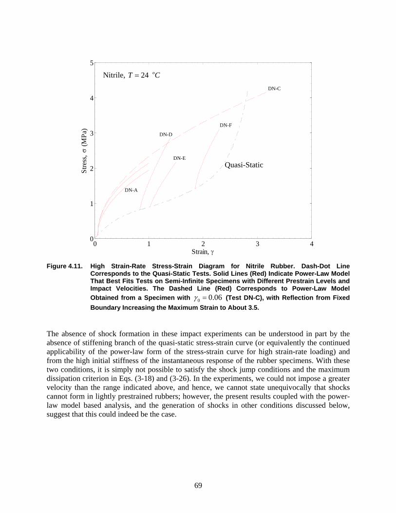
69

Figure 4.11. High Strain-Rate Stress-Strain Diagram for Nitrile Rubber. Dash-Dot Line

Corresponds to the Quasi-Static Tests. Solid Lines (Red) Indicate Power-Law Model That Best Fits Tests on Semi-Infinite Specimens with Different Prestrain Levels and Impact Velocities. The Dashed Line (Red) Corresponds to Power-Law Model Obtained from a Specimen with 0 0.06γ = (Test DN-C), with Reflection from Fixed Boundary Increasing the Maximum Strain to About 3.5.

The absence of shock formation in these impact experiments can be understood in part by the absence of stiffening branch of the quasi-static stress-strain curve (or equivalently the continued applicability of the power-law form of the stress-strain curve for high strain-rate loading) and from the high initial stiffness of the instantaneous response of the rubber specimens. With these two conditions, it is simply not possible to satisfy the shock jump conditions and the maximum dissipation criterion in Eqs. (3-18) and (3-26). In the experiments, we could not impose a greater velocity than the range indicated above, and hence, we cannot state unequivocally that shocks cannot form in lightly prestrained rubbers; however, the present results coupled with the power-law model based analysis, and the generation of shocks in other conditions discussed below, suggest that this could indeed be the case.

0 1 2 3 40

1

2

3

4

5

Strain, γ

Stre

ss, σ

(MPa

)DN-C

DN-F

DN-E

DN-D

DN-A

Quasi-Static

Nitrile, 24 oT C=

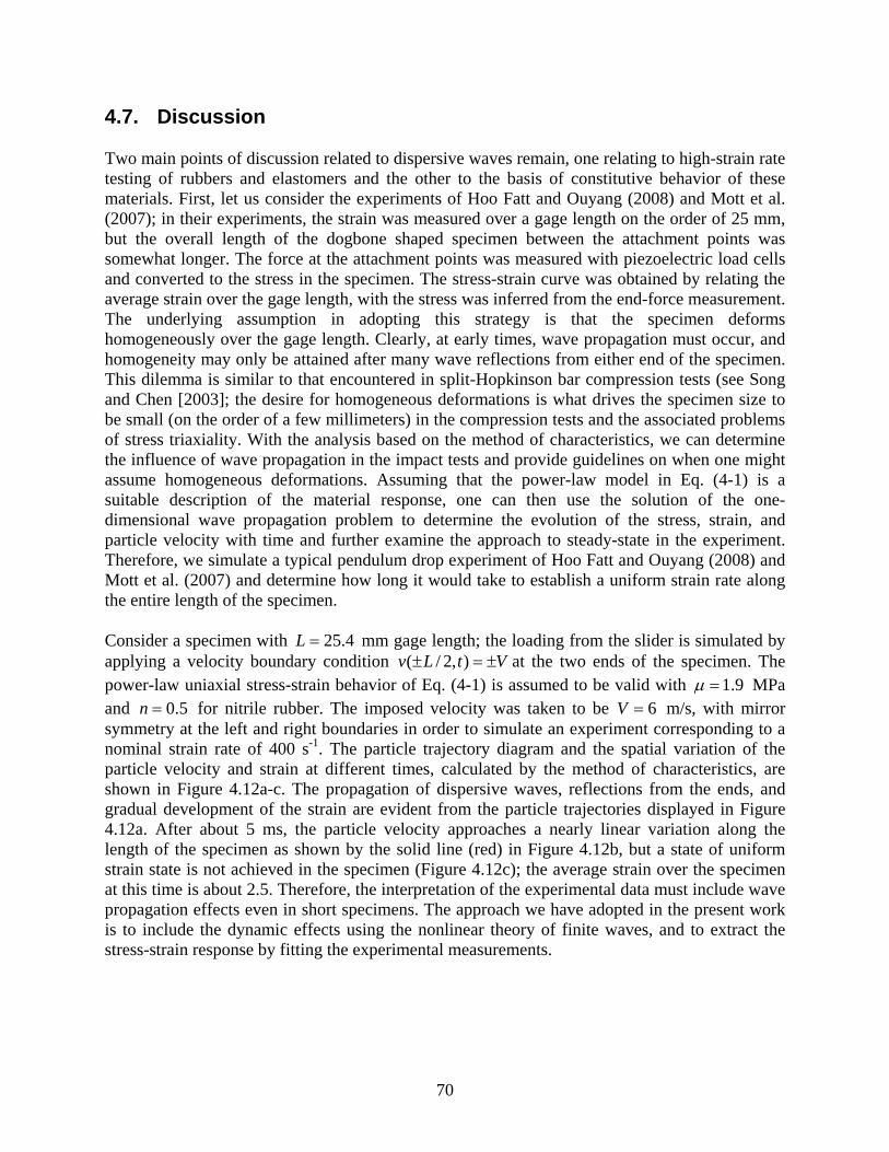
70

4.7. Discussion Two main points of discussion related to dispersive waves remain, one relating to high-strain rate testing of rubbers and elastomers and the other to the basis of constitutive behavior of these materials. First, let us consider the experiments of Hoo Fatt and Ouyang (2008) and Mott et al. (2007); in their experiments, the strain was measured over a gage length on the order of 25 mm, but the overall length of the dogbone shaped specimen between the attachment points was somewhat longer. The force at the attachment points was measured with piezoelectric load cells and converted to the stress in the specimen. The stress-strain curve was obtained by relating the average strain over the gage length, with the stress was inferred from the end-force measurement. The underlying assumption in adopting this strategy is that the specimen deforms homogeneously over the gage length. Clearly, at early times, wave propagation must occur, and homogeneity may only be attained after many wave reflections from either end of the specimen. This dilemma is similar to that encountered in split-Hopkinson bar compression tests (see Song and Chen [2003]; the desire for homogeneous deformations is what drives the specimen size to be small (on the order of a few millimeters) in the compression tests and the associated problems of stress triaxiality. With the analysis based on the method of characteristics, we can determine the influence of wave propagation in the impact tests and provide guidelines on when one might assume homogeneous deformations. Assuming that the power-law model in Eq. (4-1) is a suitable description of the material response, one can then use the solution of the one- dimensional wave propagation problem to determine the evolution of the stress, strain, and particle velocity with time and further examine the approach to steady-state in the experiment. Therefore, we simulate a typical pendulum drop experiment of Hoo Fatt and Ouyang (2008) andMott et al. (2007) and determine how long it would take to establish a uniform strain rate along the entire length of the specimen. Consider a specimen with 25.4L = mm gage length; the loading from the slider is simulated by applying a velocity boundary condition ( / 2, )v L t V± = ± at the two ends of the specimen. The power-law uniaxial stress-strain behavior of Eq. (4-1) is assumed to be valid with 1.9µ = MPa and 0.5n = for nitrile rubber. The imposed velocity was taken to be 6V = m/s, with mirror symmetry at the left and right boundaries in order to simulate an experiment corresponding to a nominal strain rate of 400 s-1. The particle trajectory diagram and the spatial variation of the particle velocity and strain at different times, calculated by the method of characteristics, are shown in Figure 4.12a-c. The propagation of dispersive waves, reflections from the ends, and gradual development of the strain are evident from the particle trajectories displayed in Figure 4.12a. After about 5 ms, the particle velocity approaches a nearly linear variation along the length of the specimen as shown by the solid line (red) in Figure 4.12b, but a state of uniform strain state is not achieved in the specimen (Figure 4.12c); the average strain over the specimen at this time is about 2.5. Therefore, the interpretation of the experimental data must include wave propagation effects even in short specimens. The approach we have adopted in the present work is to include the dynamic effects using the nonlinear theory of finite waves, and to extract the stress-strain response by fitting the experimental measurements.

71

0 0.2 0.4 0.6 0.8 1 1.2 1.4 1.6 1.8 20

1

2

3

4

5

6

Normalized position, y/L

Tim

e, t

- ms

(a)

Figure 4.12a. Particle Trajectory Diagram for Half the Specimen. Imposed Velocity on Right End

Is 6 m/s.

-0.5 -0.4 -0.3 -0.2 -0.1 0 0.1 0.2 0.3 0.4 0.5-6

-4

-2

0

2

4

6

Normalized Position, x/L

Vel

ocity

- m

/s

Figure 4.12.b Variation of Particle Velocity with Lagrangian Position at Times in the Interval of 0

to 4 ms. The Red Line Corresponds to 5.66t = ms.

72

Figure 4.12.c Variation of Strain with Lagrangian Position at Different Times in the Interval of 0 to

4 ms. The second point of discussion relates to the observed power-law model of the stress-strain response that extends to significantly large strain levels and is quite different from the typical entropic response expected of rubber from the kinetic theory. The fact that the power-law model fits the experimentally determined particle trajectories up to very large strain levels and that this model is qualitatively as well as quantitatively different from the quasi-static stress-strain response (see Figures 4.5 and 4.6) suggests that the deformation mechanisms responsible for the response must have been affected significantly. In particular, the steep increase in stiffness observed in the quasi-static experiments and associated with the non-Gaussian response of the chain extension is not replicated in the dynamic experiments, both for the latex and the nitrile rubbers. Such increase in stiffness, if present, should result in the formation of shock waves, but such shock waves were not observed in the present experiments. What are the micromechanisms of deformation of the underlying rubber network structure that result in the continued power-law response? Typically, at high Deborah number—when the time scale of the experiment is short in comparison to the relaxation times associated with monomer motion, motion of the entanglement strand, and the confining tube in the reptation model—the glassy response is elicited from the polymer; high-frequency measurements from oscillatory shear tests indicate that this is indeed the case, with the initial modulus reaching ~1 GPa, three orders of magnitude higher than the

-0.5 -0.4 -0.3 -0.2 -0.1 0 0.1 0.2 0.3 0.4 0.50

0.5

1

1.5

2

2.5

3

Normalized position, x/L

Stra

in,

γ

(c)

73

equilibrium modulus. However, these measurements are typically made at small deformations. Furthermore, as observed in the previous paragraph, it is difficult to generate large, homogeneous deformations at high strain rates because of wave propagation effects. In the present experiments, we reach strains of about 4.5 in the latex rubber and 3.2 in the nitrile rubber. Stress relaxation and large-scale chain motion of some kind must be involved in allowing such large strains to develop. Then the basis of the power-law response must be sought in this stress relaxation mechanism. We consider a very simple proposition: the glassy response brings the stress level to sufficiently high levels and relaxation of the stress by Rouse modes of the entanglement strands occurs rapidly (the Rouse time for entanglement strands is on the order of 0.1 µs, Rubenstein and Colby [2003]). If the Rouse modes are responsible for stress relaxation, then the modulus is inversely proportional to the square root of time: ( ) 1/ 2G t t−∝ .

For a constant strain rate loading, we can write this equivalently as ( ) 1/ 2G γ γ −∝ . If we interpret this relaxation modulus as the local stiffness at the strain level γ , we obtain the stress-strain behavior as ( ) 1/ 2σ γ γ∝ ; this is very close to the power-law behavior suggested by the experimental results. Of course, here we have only made heuristic arguments to motivate the power law. A more detailed examination of the mechanisms with other diagnostic tools and formulation of a molecular model would be required to motivate the power-law model appropriately. Nevertheless, these experiments suggest that the power-law model is a good representation of the instantaneous elastic response of these rubbers at high rates of stretching.

74

5. SHOCK WAVES Shock waves were formed in latex and nitrile specimens that were prestrained and impacted at high speeds. The experimental method used to generate tensile impact loading in strips of latex and nitrile rubbers is described in Section 4.1. Rubber strip specimens (thickness = 0.48 mm for latex and 0.43 mm for nitrile and width = 5 mm for both) were impacted at 0x = at velocities in the range of 17 to 65 m/s and held clamped at x L= . The motion of material points was monitored by marking lines on the specimen and following their displacement with a high-speed video camera. Particle trajectory diagrams were obtained as indicated in Section 4.1. Some of these tests indicated that a dispersive fan of waves followed the shock wave. We will first describe these experimental results and then provide an interpretation of the experiments in Section 5.3. 5.1. Impact on Rubber Specimens Generating Tensile Shocks Tensile shocks were indeed formed for 0 1γ > for the latex rubber and 0 1.5γ > for the nitrile rubber at larger impact speeds. A selected sequence of images from one test on latex rubber specimen SL-E, with a prestrain of 0 2.51γ = and impact speed of (0, ) 46v t V= − = − m/s, is shown in Figure 5.1. Black lines were drawn on the specimen at 1 mm separation in the unstretched configuration, with every fifth line identified by a thicker line. The white, dash-dot line placed across the sequence of images in Figure 5.1 identifies the position of the tensile shock at different times. Dashed white lines trace the trajectory of every fifth marker. Clearly, the constant prestrain is maintained in sector 1 in Figure 5.1, prior to the arrival of the shock; the strain increases (jumps?) to a large level in sector 2 immediately after passage of the shock. We note that the time between images is 16.7 µs, and hence, the motion of the shock is quite well resolved in the images; in fact, every sixth frame is shown in Figure 5.1 in order to show the movement of the marker lines. The complete particle trajectory diagram corresponding to Test SL-C is shown in Figure 5.2. The particles are stationary in sector 1 prior to the arrival of the shock wave whose path is indicated by the pair of dash-dot lines representing the shock width. The shock travels with a Lagrangian speed of 29s = m/s in Test SL-C. Sector 2 is immediately above the shock and represents the post-shock state. The nearly abrupt change in the particle velocity with the arrival of the shock wave is highlighted by the dashed lines that identify the right edge of the marker lines.

75

Figure 5.1. Selected Sequence of Images from Early Stages of Test SL-E. Dash-Dot Line

Indicates Trajectory of Shock Wave. Quiescent Initial State and Immediate Movement of Particles at Arrival of Shock Wave Can Be Seen in This Sequence. Shock Speed 37s = m/s and the Particle Velocity 46v− = m/s. Horizontal Resolution: 4575 Pixels per Meter. Vertical Resolution: 59,701 Pixels per Second.

These particle trajectory diagrams can be analyzed quantitatively to determine the time evolution of particle velocity, strain and strain-rate to gain an understanding of the shock response. This is accomplished by image processing and numerical differentiation as follows: first an edge tracing algorithm is used to identify the left and right edges of each particle trajectory. Next, numerical differentiation followed by smoothing (with a centered, moving-average filter) is used to determine the particle velocity and strain at fixed material points as a function of time. The time variations of the particle velocity, strain, and strain-rate for Test SL-C at points labeled A, B, C, and D in Figure 5.2 are shown in Figures 5.3, 5.4, and 5.5, respectively. From Figure 5.3 it is clear that the velocity changes quickly (within a time scale on the order of a few µs to 200 µs) from its initial value ( ,0) 0v x v+= = to about 56v− = − m/s and remains constant at this value as the shock propagates further into the specimen. There is a corresponding jump in strain from its initial value 0 1.66γ γ += = to a final value of ~ 4γ − , which can be seen in Figure 5.4; the strain also remains constant behind the shock. This strain jump can also be identified in Figure 5.1, by the rapid increase in the distance between the lines marked on the specimen with the passage of the shock. The particle velocity behind the shock coincides with the projectile velocity and hence the constant state persists beyond the arrival of the shock at any location. The time variation of

0 50 100 150 200 250 300 350

0

0.1

0.2

0.3

0.4

0.5

0.6

0.7

0.8

Position, y (pixels)

Sele

ct T

ime

Fram

es, t

(ms)

1

2

(0.076 m)

Latex, 24 oT C=

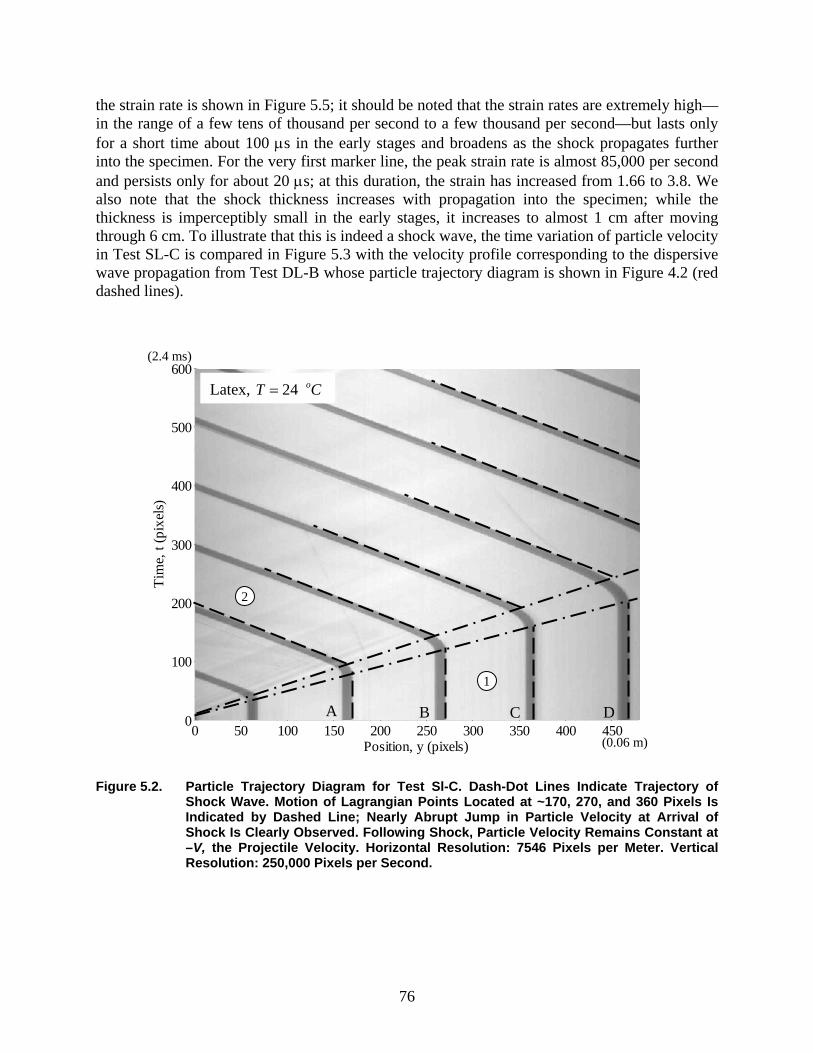
76

the strain rate is shown in Figure 5.5; it should be noted that the strain rates are extremely high—in the range of a few tens of thousand per second to a few thousand per second—but lasts only for a short time about 100 µs in the early stages and broadens as the shock propagates further into the specimen. For the very first marker line, the peak strain rate is almost 85,000 per second and persists only for about 20 µs; at this duration, the strain has increased from 1.66 to 3.8. We also note that the shock thickness increases with propagation into the specimen; while the thickness is imperceptibly small in the early stages, it increases to almost 1 cm after moving through 6 cm. To illustrate that this is indeed a shock wave, the time variation of particle velocity in Test SL-C is compared in Figure 5.3 with the velocity profile corresponding to the dispersive wave propagation from Test DL-B whose particle trajectory diagram is shown in Figure 4.2 (red dashed lines).

Figure 5.2. Particle Trajectory Diagram for Test Sl-C. Dash-Dot Lines Indicate Trajectory of

Shock Wave. Motion of Lagrangian Points Located at ~170, 270, and 360 Pixels Is Indicated by Dashed Line; Nearly Abrupt Jump in Particle Velocity at Arrival of Shock Is Clearly Observed. Following Shock, Particle Velocity Remains Constant at –V, the Projectile Velocity. Horizontal Resolution: 7546 Pixels per Meter. Vertical Resolution: 250,000 Pixels per Second.

(2.4 ms)

(0.06 m) 0 50 100 150 200 250 300 350 400 450

0

100

200

300

400

500

600

Position, y (pixels)

Tim

e, t

(pix

els)

1

2

A B C D

Latex, 24 oT C=

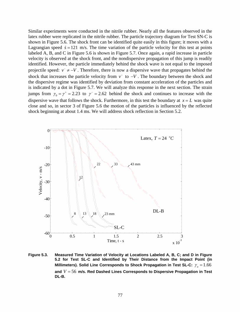
77

Similar experiments were conducted in the nitrile rubber. Nearly all the features observed in the latex rubber were replicated in the nitrile rubber. The particle trajectory diagram for Test SN-C is shown in Figure 5.6. The shock front can be identified quite easily in this figure; it moves with a Lagrangian speed 121s = m/s. The time variation of the particle velocity for this test at points labeled A, B, and C in Figure 5.6 is shown in Figure 5.7. Once again, a rapid increase in particle velocity is observed at the shock front, and the nondispersive propagation of this jump is readily identified. However, the particle immediately behind the shock wave is not equal to the imposed projectile speed: v V− ≠ − . Therefore, there is now a dispersive wave that propagates behind the shock that increases the particle velocity from v− to V− . The boundary between the shock and the dispersive regime was identified by deviation from constant acceleration of the particles and is indicated by a dot in Figure 5.7. We will analyze this response in the next section. The strain jumps from 0 2.23γ γ += = to 2.62γ − = behind the shock and continues to increase with the dispersive wave that follows the shock. Furthermore, in this test the boundary at x L= was quite close and so, in sector 3 of Figure 5.6 the motion of the particles is influenced by the reflected shock beginning at about 1.4 ms. We will address shock reflection in Section 5.2.

Figure 5.3. Measured Time Variation of Velocity at Locations Labeled A, B, C; and D in Figure

5.2 for Test SL-C and Identified by Their Distance from the Impact Point (in Millimeters). Solid Line Corresponds to Shock Propagation in Test SL-C: 1.66oγ = and 56V = m/s. Red Dashed Lines Corresponds to Dispersive Propagation in Test DL-B.

0 0.5 1 1.5 2 2.5 3x 10

-3

-60

-50

-40

-30

-20

-10

0

Time, t - s

Vel

ocity

, v -

m/s

12

22 33 43 mm

8 13 18 23 mm

SL-C

DL-B

Latex, 24 oT C=

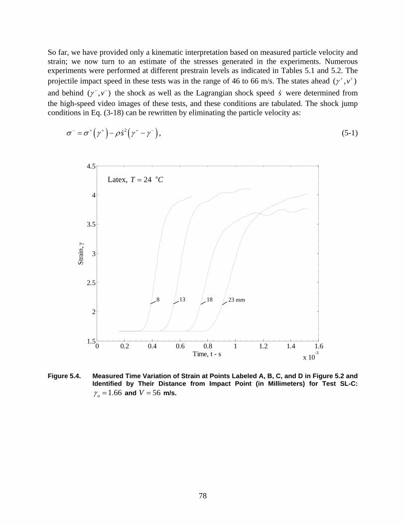
78

So far, we have provided only a kinematic interpretation based on measured particle velocity and strain; we now turn to an estimate of the stresses generated in the experiments. Numerous experiments were performed at different prestrain levels as indicated in Tables 5.1 and 5.2. The projectile impact speed in these tests was in the range of 46 to 66 m/s. The states ahead ( , )vγ + + and behind ( , )vγ − − the shock as well as the Lagrangian shock speed s were determined from the high-speed video images of these tests, and these conditions are tabulated. The shock jump conditions in Eq. (3-18) can be rewritten by eliminating the particle velocity as:

( ) ( )2sσ σ γ ρ γ γ− + + + −= − − , (5-1)

Figure 5.4. Measured Time Variation of Strain at Points Labeled A, B, C, and D in Figure 5.2 and

Identified by Their Distance from Impact Point (in Millimeters) for Test SL-C: 1.66oγ = and 56V = m/s.

0 0.2 0.4 0.6 0.8 1 1.2 1.4 1.6x 10

-3

1.5

2

2.5

3

3.5

4

4.5

Time, t - s

Stra

in, γ

8 13 18 23 mm

Latex, 24 oT C=

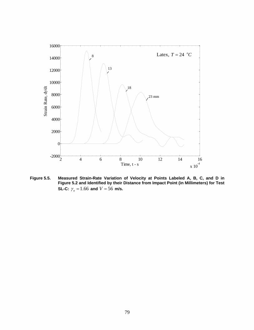
79

Figure 5.5. Measured Strain-Rate Variation of Velocity at Points Labeled A, B, C, and D in

Figure 5.2 and Identified by their Distance from Impact Point (in Millimeters) for Test SL-C: 1.66oγ = and 56V = m/s.

2 4 6 8 10 12 14 16x 10

-4

-2000

0

2000

4000

6000

8000

10000

12000

14000

16000

Time, t - s

Stra

in R

ate,

dγ /d

t

8

13

18

23 mm

Latex, 24 oT C=

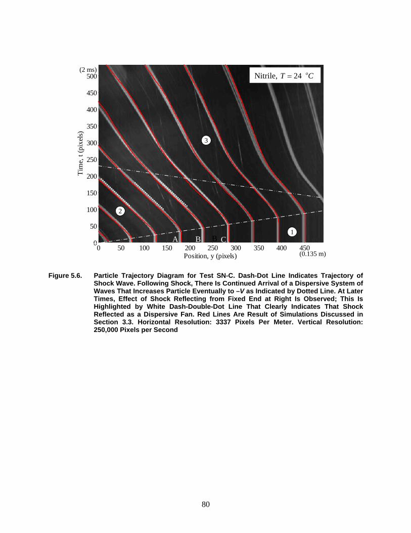
80

Figure 5.6. Particle Trajectory Diagram for Test SN-C. Dash-Dot Line Indicates Trajectory of

Shock Wave. Following Shock, There Is Continued Arrival of a Dispersive System of Waves That Increases Particle Eventually to –V as Indicated by Dotted Line. At Later Times, Effect of Shock Reflecting from Fixed End at Right Is Observed; This Is Highlighted by White Dash-Double-Dot Line That Clearly Indicates That Shock Reflected as a Dispersive Fan. Red Lines Are Result of Simulations Discussed in Section 3.3. Horizontal Resolution: 3337 Pixels Per Meter. Vertical Resolution: 250,000 Pixels per Second

0 50 100 150 200 250 300 350 400 4500

50

100

150

200

250

300

350

400

450

500

Position, y (pixels)

Tim

e, t

(pix

els)

1

2

3

B A B C

(2 ms)

(0.135 m)

Nitrile, 24 oT C=

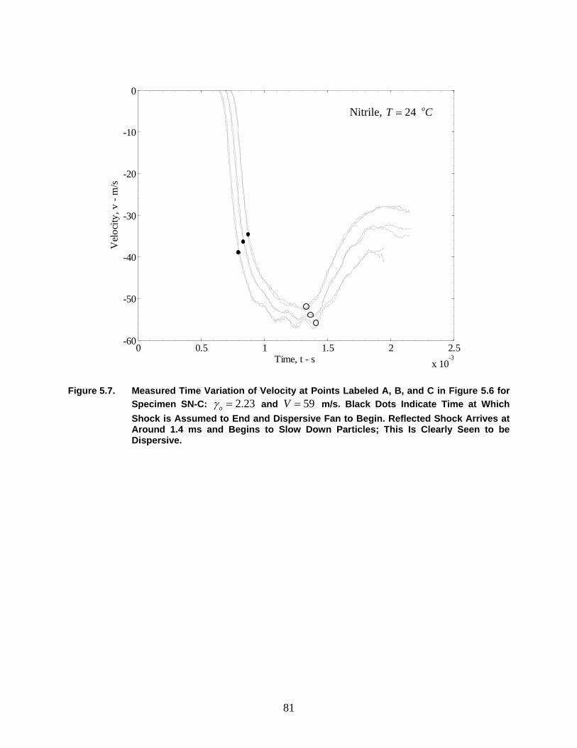
81

Figure 5.7. Measured Time Variation of Velocity at Points Labeled A, B, and C in Figure 5.6 for

Specimen SN-C: 2.23oγ = and 59V = m/s. Black Dots Indicate Time at Which Shock is Assumed to End and Dispersive Fan to Begin. Reflected Shock Arrives at Around 1.4 ms and Begins to Slow Down Particles; This Is Clearly Seen to be Dispersive.

0 0.5 1 1.5 2 2.5x 10

-3

-60

-50

-40

-30

-20

-10

0

Time, t - s

Vel

ocity

, v -

m/s

Nitrile, 24 oT C=

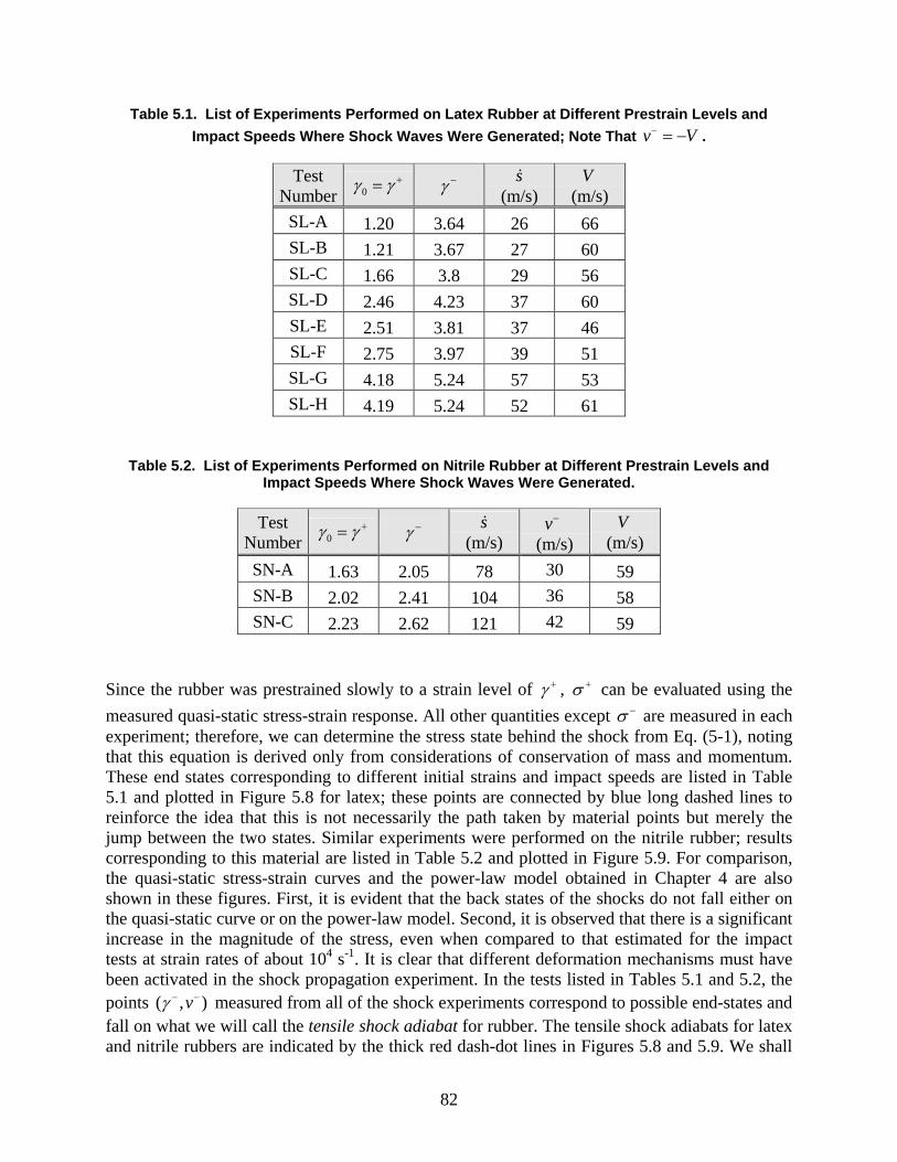
82

Table 5.1. List of Experiments Performed on Latex Rubber at Different Prestrain Levels and Impact Speeds Where Shock Waves Were Generated; Note That v V− = − .

Test Number 0γ γ += γ − s

(m/s) V

(m/s) SL-A 1.20 3.64 26 66 SL-B 1.21 3.67 27 60 SL-C 1.66 3.8 29 56 SL-D 2.46 4.23 37 60 SL-E 2.51 3.81 37 46 SL-F 2.75 3.97 39 51 SL-G 4.18 5.24 57 53 SL-H 4.19 5.24 52 61

Table 5.2. List of Experiments Performed on Nitrile Rubber at Different Prestrain Levels and Impact Speeds Where Shock Waves Were Generated.

Test Number 0γ γ += γ − s

(m/s) v−

(m/s) V

(m/s) SN-A 1.63 2.05 78 30 59 SN-B 2.02 2.41 104 36 58 SN-C 2.23 2.62 121 42 59

Since the rubber was prestrained slowly to a strain level of γ + , σ + can be evaluated using the measured quasi-static stress-strain response. All other quantities except σ − are measured in each experiment; therefore, we can determine the stress state behind the shock from Eq. (5-1), noting that this equation is derived only from considerations of conservation of mass and momentum. These end states corresponding to different initial strains and impact speeds are listed in Table 5.1 and plotted in Figure 5.8 for latex; these points are connected by blue long dashed lines to reinforce the idea that this is not necessarily the path taken by material points but merely the jump between the two states. Similar experiments were performed on the nitrile rubber; results corresponding to this material are listed in Table 5.2 and plotted in Figure 5.9. For comparison, the quasi-static stress-strain curves and the power-law model obtained in Chapter 4 are also shown in these figures. First, it is evident that the back states of the shocks do not fall either on the quasi-static curve or on the power-law model. Second, it is observed that there is a significant increase in the magnitude of the stress, even when compared to that estimated for the impact tests at strain rates of about 104 s-1. It is clear that different deformation mechanisms must have been activated in the shock propagation experiment. In the tests listed in Tables 5.1 and 5.2, the points ( , )vγ − − measured from all of the shock experiments correspond to possible end-states and fall on what we will call the tensile shock adiabat for rubber. The tensile shock adiabats for latex and nitrile rubbers are indicated by the thick red dash-dot lines in Figures 5.8 and 5.9. We shall

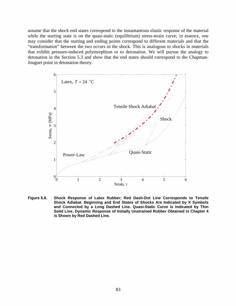
83

assume that the shock end states correspond to the instantaneous elastic response of the material while the starting state is on the quasi-static (equilibrium) stress-strain curve; in essence, one may consider that the starting and ending points correspond to different materials and that the “transformation” between the two occurs in the shock. This is analogous to shocks in materials that exhibit pressure-induced polymorphism or to detonation. We will pursue the analogy to detonation in the Section 5.3 and show that the end states should correspond to the Chapman-Jouguet point in detonation theory.

Figure 5.8. Shock Response of Latex Rubber; Red Dash-Dot Line Corresponds to Tensile

Shock Adiabat. Beginning and End States of Shocks Are Indicated by X Symbols and Connected by a Long Dashed Line. Quasi-Static Curve Is Indicated by Thin Solid Line. Dynamic Response of Initially Unstrained Rubber Obtained in Chapter 4 is Shown by Red Dashed Line.

0 1 2 3 4 5 60

1

2

3

4

5

6

Strain, γ

Stre

ss, σ

(MPa

)

Latex, 24 oT C=

Power-Law

Tensile Shock Adiabat

Shock

Quasi-Static

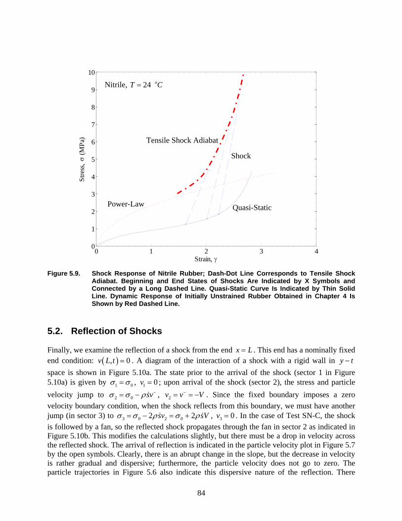
84

Figure 5.9. Shock Response of Nitrile Rubber; Dash-Dot Line Corresponds to Tensile Shock

Adiabat. Beginning and End States of Shocks Are Indicated by X Symbols and Connected by a Long Dashed Line. Quasi-Static Curve Is Indicated by Thin Solid Line. Dynamic Response of Initially Unstrained Rubber Obtained in Chapter 4 Is Shown by Red Dashed Line.

5.2. Reflection of Shocks Finally, we examine the reflection of a shock from the end x L= . This end has a nominally fixed end condition: ( ), 0v L t = . A diagram of the interaction of a shock with a rigid wall in y t− space is shown in Figure 5.10a. The state prior to the arrival of the shock (sector 1 in Figure 5.10a) is given by 1 0σ σ= , 1 0v = ; upon arrival of the shock (sector 2), the stress and particle velocity jump to 2 0 svσ σ ρ −= − , 2v v V−= = − . Since the fixed boundary imposes a zero velocity boundary condition, when the shock reflects from this boundary, we must have another jump (in sector 3) to 3 0 2 02 2sv sVσ σ ρ σ ρ= − = + , 3 0v = . In the case of Test SN-C, the shock is followed by a fan, so the reflected shock propagates through the fan in sector 2 as indicated in Figure 5.10b. This modifies the calculations slightly, but there must be a drop in velocity across the reflected shock. The arrival of reflection is indicated in the particle velocity plot in Figure 5.7 by the open symbols. Clearly, there is an abrupt change in the slope, but the decrease in velocity is rather gradual and dispersive; furthermore, the particle velocity does not go to zero. The particle trajectories in Figure 5.6 also indicate this dispersive nature of the reflection. There

0 1 2 3 40

1

2

3

4

5

6

7

8

9

10

Strain, γ

Stre

ss, σ

(MPa

)Nitrile, 24 oT C=

Power-Law

Tensile Shock Adiabat

Shock

Quasi-Static

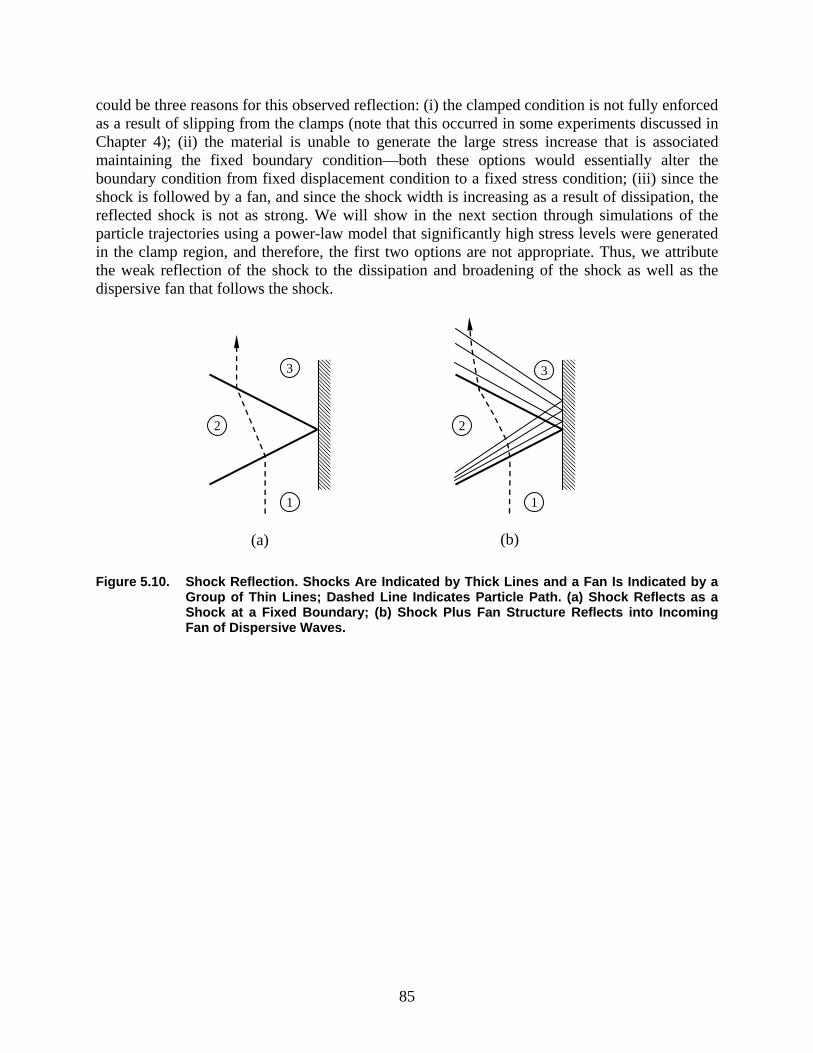
85

could be three reasons for this observed reflection: (i) the clamped condition is not fully enforced as a result of slipping from the clamps (note that this occurred in some experiments discussed in Chapter 4); (ii) the material is unable to generate the large stress increase that is associated maintaining the fixed boundary condition—both these options would essentially alter the boundary condition from fixed displacement condition to a fixed stress condition; (iii) since the shock is followed by a fan, and since the shock width is increasing as a result of dissipation, the reflected shock is not as strong. We will show in the next section through simulations of the particle trajectories using a power-law model that significantly high stress levels were generated in the clamp region, and therefore, the first two options are not appropriate. Thus, we attribute the weak reflection of the shock to the dissipation and broadening of the shock as well as the dispersive fan that follows the shock.

Figure 5.10. Shock Reflection. Shocks Are Indicated by Thick Lines and a Fan Is Indicated by a

Group of Thin Lines; Dashed Line Indicates Particle Path. (a) Shock Reflects as a Shock at a Fixed Boundary; (b) Shock Plus Fan Structure Reflects into Incoming Fan of Dispersive Waves.

1

2

3

1

2

3

(a) (b)

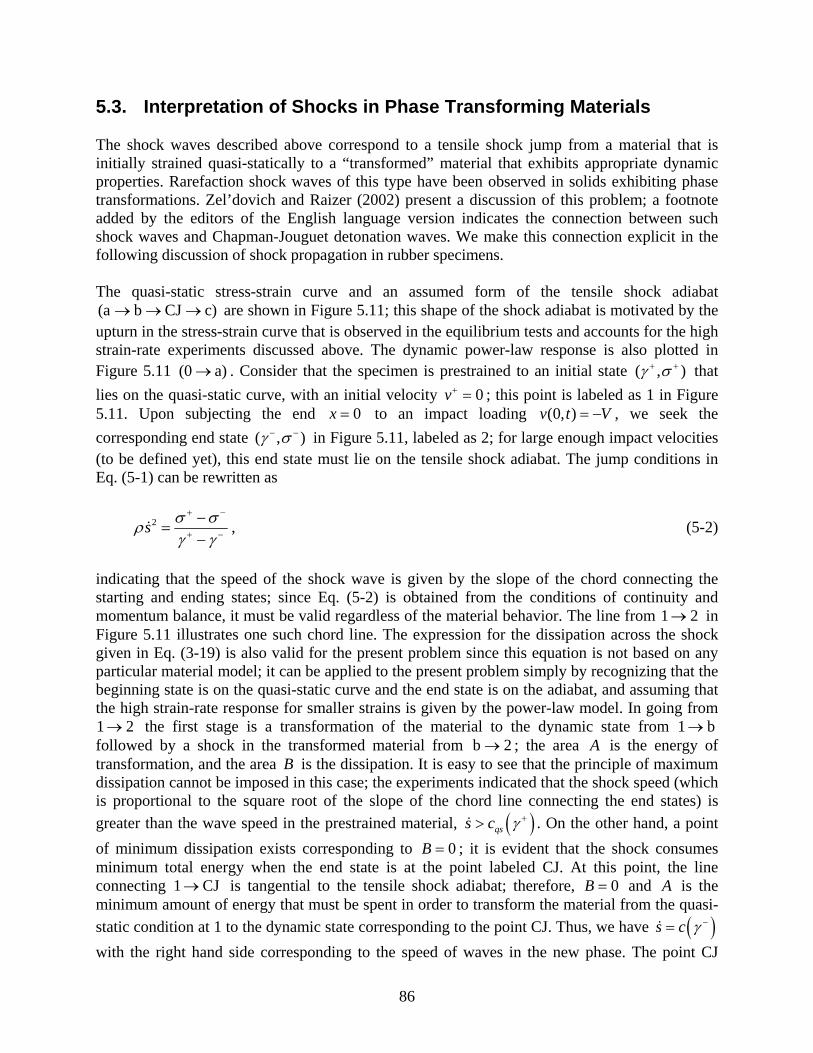
86

5.3. Interpretation of Shocks in Phase Transforming Materials The shock waves described above correspond to a tensile shock jump from a material that is initially strained quasi-statically to a “transformed” material that exhibits appropriate dynamic properties. Rarefaction shock waves of this type have been observed in solids exhibiting phase transformations. Zel’dovich and Raizer (2002) present a discussion of this problem; a footnote added by the editors of the English language version indicates the connection between such shock waves and Chapman-Jouguet detonation waves. We make this connection explicit in the following discussion of shock propagation in rubber specimens. The quasi-static stress-strain curve and an assumed form of the tensile shock adiabat (a b CJ c)→ → → are shown in Figure 5.11; this shape of the shock adiabat is motivated by the upturn in the stress-strain curve that is observed in the equilibrium tests and accounts for the high strain-rate experiments discussed above. The dynamic power-law response is also plotted in Figure 5.11 (0 a)→ . Consider that the specimen is prestrained to an initial state ( , )γ σ+ + that lies on the quasi-static curve, with an initial velocity 0v+ = ; this point is labeled as 1 in Figure 5.11. Upon subjecting the end 0x = to an impact loading (0, )v t V= − , we seek the corresponding end state ( , )γ σ− − in Figure 5.11, labeled as 2; for large enough impact velocities (to be defined yet), this end state must lie on the tensile shock adiabat. The jump conditions in Eq. (5-1) can be rewritten as

2s σ σργ γ

+ −

+ −

−=

−, (5-2)

indicating that the speed of the shock wave is given by the slope of the chord connecting the starting and ending states; since Eq. (5-2) is obtained from the conditions of continuity and momentum balance, it must be valid regardless of the material behavior. The line from 1 2→ in Figure 5.11 illustrates one such chord line. The expression for the dissipation across the shock given in Eq. (3-19) is also valid for the present problem since this equation is not based on any particular material model; it can be applied to the present problem simply by recognizing that the beginning state is on the quasi-static curve and the end state is on the adiabat, and assuming that the high strain-rate response for smaller strains is given by the power-law model. In going from 1 2→ the first stage is a transformation of the material to the dynamic state from 1 b→ followed by a shock in the transformed material from b 2→ ; the area A is the energy of transformation, and the area B is the dissipation. It is easy to see that the principle of maximum dissipation cannot be imposed in this case; the experiments indicated that the shock speed (which is proportional to the square root of the slope of the chord line connecting the end states) is greater than the wave speed in the prestrained material, ( )qss c γ +> . On the other hand, a point of minimum dissipation exists corresponding to 0B = ; it is evident that the shock consumes minimum total energy when the end state is at the point labeled CJ. At this point, the line connecting 1 CJ→ is tangential to the tensile shock adiabat; therefore, 0B = and A is the minimum amount of energy that must be spent in order to transform the material from the quasi-static condition at 1 to the dynamic state corresponding to the point CJ. Thus, we have ( )s c γ −= with the right hand side corresponding to the speed of waves in the new phase. The point CJ

87

corresponds to the Chapman-Jouguet point in the theory of detonation. Now we see that the tensile shock adiabat can be constructed by performing impact experiments at different prestrain levels, obtaining the shock end states, and then drawing the curve that is tangent to all these chord lines. Such a construction of the shock adiabat is shown in Figures 5.8 and 5.9 for the latex and nitrile rubbers respectively by the thick dash-dot lines.

Figure 5.11. Construction of Shock Jump Diagram. Initial State of a Material Point Is at 1 on

Quasi-Static Curve. Upon Impact, End State Jumps Behind Shock to Some Point 2. Minimum Energy Is Consumed when End State Is at Point CJ Such That Line 1 CJ→ Is Tangent to Tensile Shock Adiabat.

Corresponding to any particular value of initial strain Iγ , there is an impact velocity

I

CJVγ that will result in exactly the appropriate value of CJγ behind the shock; this value can be calculated for any given starting strain, if the corresponding shock adiabat is known by drawing a line from ( ),I Iγ σ on the quasi-static curve that is tangent to the shock adiabat. However, now the following question arises: since we impose the velocity from an external source, this velocity may be greater, smaller, or equal to

I

CJVγ . How does the rubber respond to different imposed velocities? In the theory of detonation, as discussed by Landau and Lifshitz (2004), shocks of greater speed (and hence greater pressure jump) can be imposed externally, but self-propagating detonation shocks will always correspond to CJ detonation propagating at the appropriate speed. Similarly, in the case of tensile impact on rubber, if an impact velocity greater than that corresponding to the CJ point is imposed,

I

CJV Vγ> , one expects that a CJ shock occurs and is then followed by dispersive waves that correspond to the propagation of waves in the

Strain, γ

Stre

ss, σ

2

1

b CJ

B

A

a

c

Quasi-Static Power-Law

Tensile Shock Adiabat

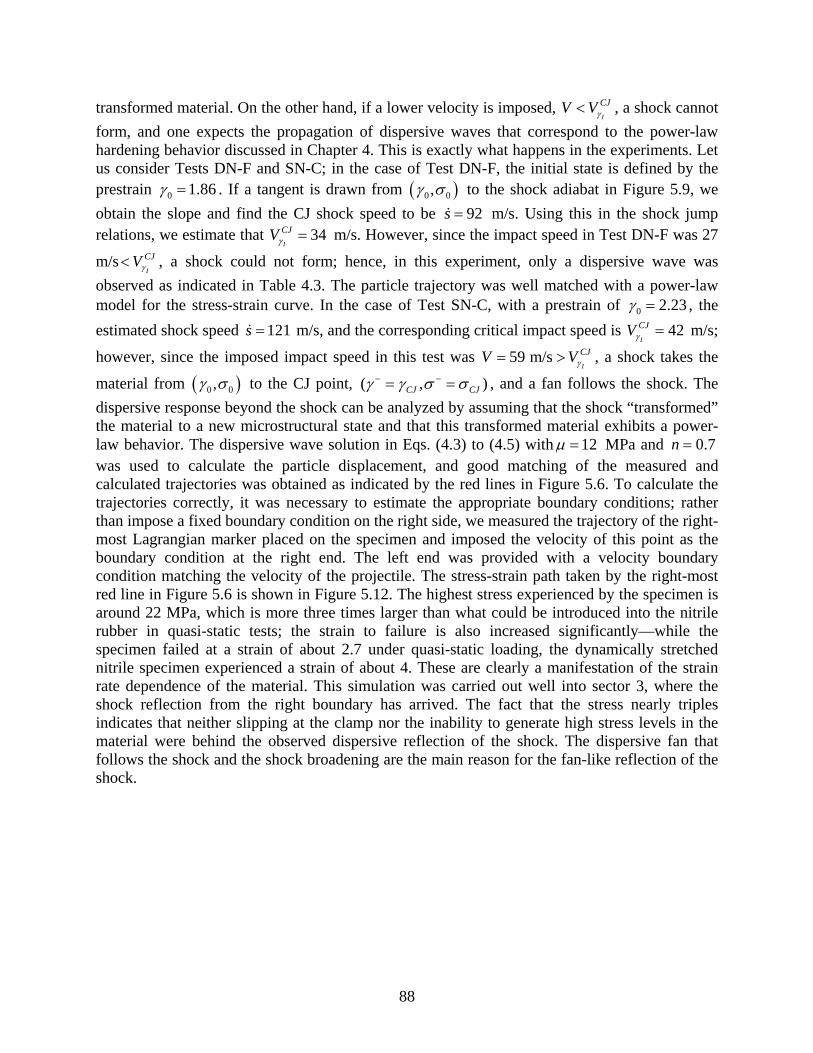
88

transformed material. On the other hand, if a lower velocity is imposed, I

CJV Vγ< , a shock cannot form, and one expects the propagation of dispersive waves that correspond to the power-law hardening behavior discussed in Chapter 4. This is exactly what happens in the experiments. Let us consider Tests DN-F and SN-C; in the case of Test DN-F, the initial state is defined by the prestrain 0 1.86γ = . If a tangent is drawn from ( )0 0,γ σ to the shock adiabat in Figure 5.9, we obtain the slope and find the CJ shock speed to be 92s = m/s. Using this in the shock jump relations, we estimate that 34

I

CJVγ = m/s. However, since the impact speed in Test DN-F was 27

m/sI

CJVγ< , a shock could not form; hence, in this experiment, only a dispersive wave was observed as indicated in Table 4.3. The particle trajectory was well matched with a power-law model for the stress-strain curve. In the case of Test SN-C, with a prestrain of 0 2.23γ = , the estimated shock speed 121s = m/s, and the corresponding critical impact speed is 42

I

CJVγ = m/s;

however, since the imposed impact speed in this test was 59 m/sI

CJV Vγ= > , a shock takes the

material from ( )0 0,γ σ to the CJ point, ( , )CJ CJγ γ σ σ− −= = , and a fan follows the shock. The dispersive response beyond the shock can be analyzed by assuming that the shock “transformed” the material to a new microstructural state and that this transformed material exhibits a power-law behavior. The dispersive wave solution in Eqs. (4.3) to (4.5) with 12µ = MPa and 0.7n = was used to calculate the particle displacement, and good matching of the measured and calculated trajectories was obtained as indicated by the red lines in Figure 5.6. To calculate the trajectories correctly, it was necessary to estimate the appropriate boundary conditions; rather than impose a fixed boundary condition on the right side, we measured the trajectory of the right-most Lagrangian marker placed on the specimen and imposed the velocity of this point as the boundary condition at the right end. The left end was provided with a velocity boundary condition matching the velocity of the projectile. The stress-strain path taken by the right-most red line in Figure 5.6 is shown in Figure 5.12. The highest stress experienced by the specimen is around 22 MPa, which is more three times larger than what could be introduced into the nitrile rubber in quasi-static tests; the strain to failure is also increased significantly—while the specimen failed at a strain of about 2.7 under quasi-static loading, the dynamically stretched nitrile specimen experienced a strain of about 4. These are clearly a manifestation of the strain rate dependence of the material. This simulation was carried out well into sector 3, where the shock reflection from the right boundary has arrived. The fact that the stress nearly triples indicates that neither slipping at the clamp nor the inability to generate high stress levels in the material were behind the observed dispersive reflection of the shock. The dispersive fan that follows the shock and the shock broadening are the main reason for the fan-like reflection of the shock.

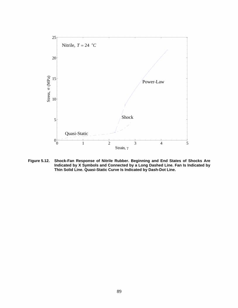
89

Figure 5.12. Shock-Fan Response of Nitrile Rubber. Beginning and End States of Shocks Are

Indicated by X Symbols and Connected by a Long Dashed Line. Fan Is Indicated by Thin Solid Line. Quasi-Static Curve Is Indicated by Dash-Dot Line.

0 1 2 3 4 50

5

10

15

20

25

Strain, γ

Stre

ss, σ

(MPa

)Nitrile, 24 oT C=

Quasi-Static

Shock

Power-Law

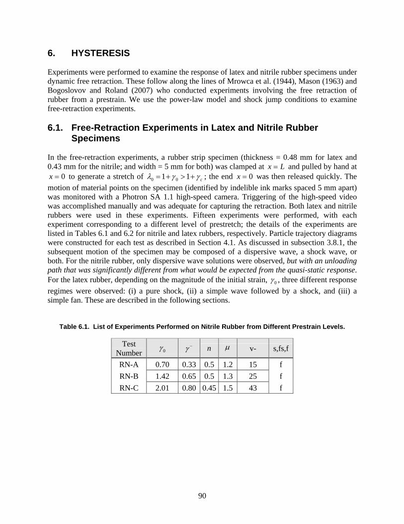
90

6. HYSTERESIS Experiments were performed to examine the response of latex and nitrile rubber specimens under dynamic free retraction. These follow along the lines of Mrowca et al. (1944), Mason (1963) and Bogoslovov and Roland (2007) who conducted experiments involving the free retraction of rubber from a prestrain. We use the power-law model and shock jump conditions to examine free-retraction experiments. 6.1. Free-Retraction Experiments in Latex and Nitrile Rubber

Specimens In the free-retraction experiments, a rubber strip specimen (thickness = 0.48 mm for latex and 0.43 mm for the nitrile; and width = 5 mm for both) was clamped at Lx = and pulled by hand at

0=x to generate a stretch of 0 01 1 cλ γ γ= + > + ; the end 0=x was then released quickly. The motion of material points on the specimen (identified by indelible ink marks spaced 5 mm apart) was monitored with a Photron SA 1.1 high-speed camera. Triggering of the high-speed video was accomplished manually and was adequate for capturing the retraction. Both latex and nitrile rubbers were used in these experiments. Fifteen experiments were performed, with each experiment corresponding to a different level of prestretch; the details of the experiments are listed in Tables 6.1 and 6.2 for nitrile and latex rubbers, respectively. Particle trajectory diagrams were constructed for each test as described in Section 4.1. As discussed in subsection 3.8.1, the subsequent motion of the specimen may be composed of a dispersive wave, a shock wave, or both. For the nitrile rubber, only dispersive wave solutions were observed, but with an unloading path that was significantly different from what would be expected from the quasi-static response. For the latex rubber, depending on the magnitude of the initial strain, 0γ , three different response regimes were observed: (i) a pure shock, (ii) a simple wave followed by a shock, and (iii) a simple fan. These are described in the following sections.

Table 6.1. List of Experiments Performed on Nitrile Rubber from Different Prestrain Levels.

Test Number 0γ γ − n µ v- s,fs,f

RN-A 0.70 0.33 0.5 1.2 15 f RN-B 1.42 0.65 0.5 1.3 25 f RN-C 2.01 0.80 0.45 1.5 43 f

91

Table 6.2. List of Experiments Performed on Latex Rubber from Different Prestrain Levels.

Test Number 0γ s

(m/s) γ + γ − n µ v+ v− σ + (MPa)

0σ (MPa)

s,fs,f

RL-A 0.5 34.6 - 0.09 - - 0 14.2 0.471 0.471 s RL-B 1.08 28.8 - 0.1 - - 0 26.7 0.735 0.735 s RL-C 2.19 22.8 1.52 0.16 0.7 0.63 18 44.5 0.677 1.153 fs RL-D 2.67 21.2 1.68 0.2 0.6 0.7 26 50 0.624 1.320 fs RL-E 2.68 21 1.7 0.18 0.6 0.7 26 54 0.644 1.335 fs RL-F 3.1 26 2.0 0.23 0.6 0.6 26 54.5 0.614 1.249 fs RL-G 3.56 17.12 2.0 0.22 0.5 0.7 36 64 0.499 1.373 fs RL-H 3.94 14.1 2.3 0.15 0.65 0.35 28 55.8 0.411 0.894 fs RL-I 3.95 13.72 2.3 0.27 0.55 0.41 29 57 0.366 0.906 fs RL-J 4.23 13.36 2.1 0.26 0.45 0.575 39 64 0.314 1.122 fs RL-K 4.75 - - 0.34 0.35 0.8 - 71.2 - 1.345 f RL-L 5.06 - - 0.39 0.3 0.95 - 75 - 1.508 f

6.2. Power-Law Model for Free-Retraction While the cubic material model indicates all the qualitative features that are expected in the retraction experiment—generation of a dispersive fan followed by a shock jump—it was not possible to match the experimental observations with this model because of the hysteretic response of the material. Numerical representations of the measured quasi-static response were also not adequate for a quantitative comparison with the experiments. To provide quantitative comparisons, we use the power-law model for determining the unloading response; the use of the power-law model is motivated by the fact that this was quite successful in capturing the loading response as well as by the fact that it exhibits a rapid drop in stress without attendant decrease in the strain, mimicking the instantaneous elastic response observed under loading.

We take a phenomenological approach and postulate a possible unloading stress-strain response for the material that could produce dispersive waves as well as shock waves. We do not attempt to motivate this form of the response from micromechanics of deformation of the polymer chains. We use a power-law model of the form given below that allows for the possibility of extremely fast initial wave speeds:

( )0 0rn

rσ σ µ γ γ= − − , (6-1)

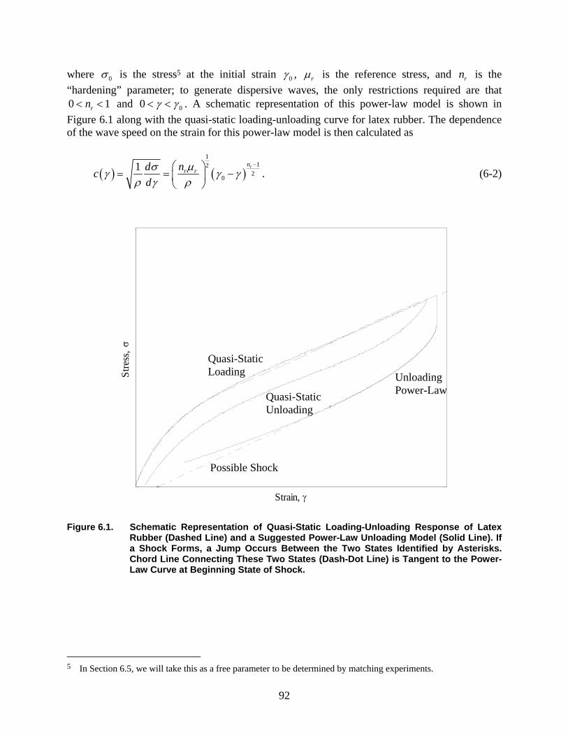
92

where 0σ is the stress5 at the initial strain 0γ , rµ is the reference stress, and rn is the “hardening” parameter; to generate dispersive waves, the only restrictions required are that 0 1rn< < and 00 γ γ< < . A schematic representation of this power-law model is shown in Figure 6.1 along with the quasi-static loading-unloading curve for latex rubber. The dependence of the wave speed on the strain for this power-law model is then calculated as

( ) ( )1

122

01 rn

r rndcd

µσγ γ γρ γ ρ

−⎛ ⎞= = −⎜ ⎟

⎝ ⎠. (6-2)

Figure 6.1. Schematic Representation of Quasi-Static Loading-Unloading Response of Latex

Rubber (Dashed Line) and a Suggested Power-Law Unloading Model (Solid Line). If a Shock Forms, a Jump Occurs Between the Two States Identified by Asterisks. Chord Line Connecting These Two States (Dash-Dot Line) is Tangent to the Power-Law Curve at Beginning State of Shock.

5 In Section 6.5, we will take this as a free parameter to be determined by matching experiments.

Strain, γ

Stre

ss, σ

Quasi-Static Loading Unloading

Power-Law

Possible Shock

Quasi-Static Unloading

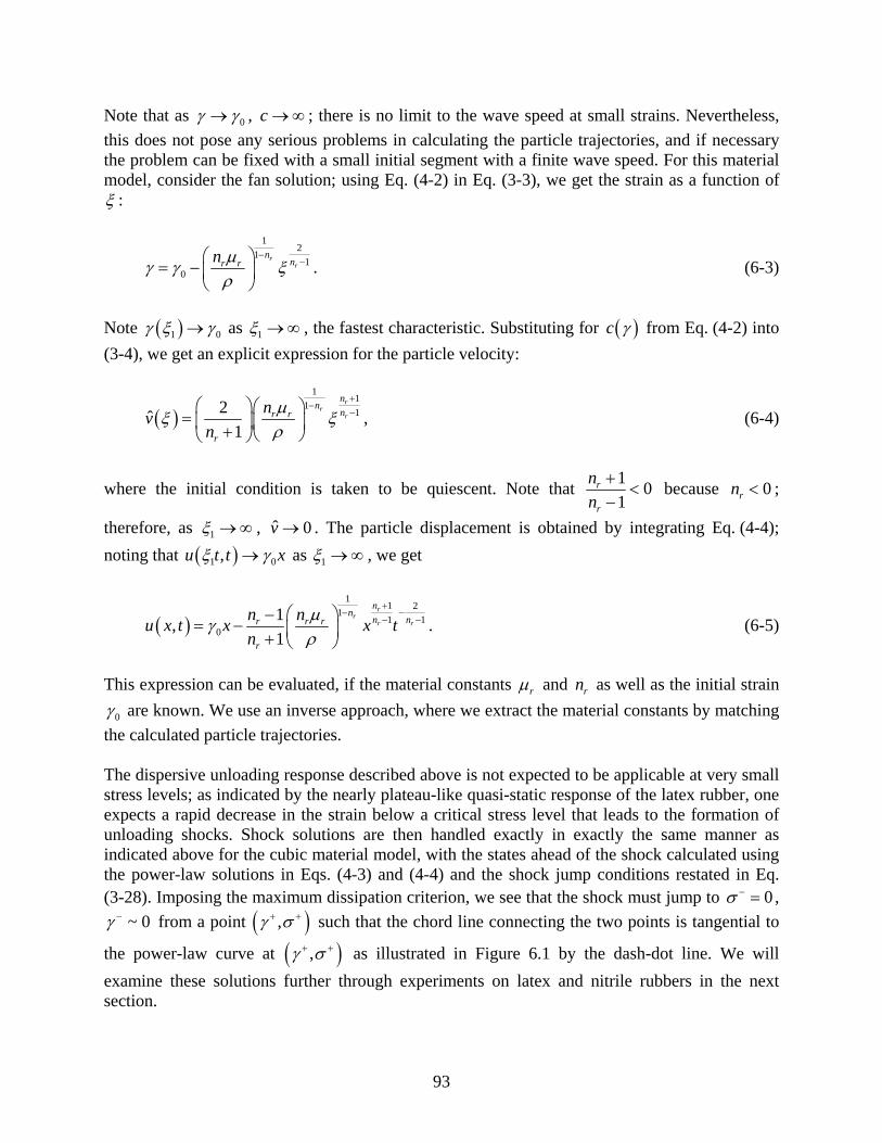
93

Note that as 0γ γ→ , c → ∞ ; there is no limit to the wave speed at small strains. Nevertheless, this does not pose any serious problems in calculating the particle trajectories, and if necessary the problem can be fixed with a small initial segment with a finite wave speed. For this material model, consider the fan solution; using Eq. (4-2) in Eq. (3-3), we get the strain as a function of ξ :

12

11

0

rr

nnr rn µγ γ ξ

ρ

−−⎛ ⎞

= − ⎜ ⎟⎝ ⎠

. (6-3)

Note ( )1 0γ ξ γ→ as 1ξ → ∞ , the fastest characteristic. Substituting for ( )c γ from Eq. (4-2) into (3-4), we get an explicit expression for the particle velocity:

( )1

11

12ˆ1

rr

r

nn

nr r

r

nvn

µξ ξρ

+−

−⎛ ⎞⎛ ⎞= ⎜ ⎟⎜ ⎟+ ⎝ ⎠⎝ ⎠

, (6-4)

where the initial condition is taken to be quiescent. Note that 1 01

r

r

nn

+<

− because 0rn < ;

therefore, as 1ξ → ∞ , ˆ 0v → . The particle displacement is obtained by integrating Eq. (4-4); noting that ( )1 0,u t t xξ γ→ as 1ξ → ∞ , we get

( )1

1 21

1 10

1,1

rr

r r

nn

n nr r r

r

n nu x t x x tn

µγρ

+−−

− −⎛ ⎞−= − ⎜ ⎟+ ⎝ ⎠

. (6-5)

This expression can be evaluated, if the material constants rµ and rn as well as the initial strain

0γ are known. We use an inverse approach, where we extract the material constants by matching the calculated particle trajectories. The dispersive unloading response described above is not expected to be applicable at very small stress levels; as indicated by the nearly plateau-like quasi-static response of the latex rubber, one expects a rapid decrease in the strain below a critical stress level that leads to the formation of unloading shocks. Shock solutions are then handled exactly in exactly the same manner as indicated above for the cubic material model, with the states ahead of the shock calculated using the power-law solutions in Eqs. (4-3) and (4-4) and the shock jump conditions restated in Eq. (3-28). Imposing the maximum dissipation criterion, we see that the shock must jump to 0σ − = ,

~ 0γ − from a point ( ),γ σ+ + such that the chord line connecting the two points is tangential to

the power-law curve at ( ),γ σ+ + as illustrated in Figure 6.1 by the dash-dot line. We will examine these solutions further through experiments on latex and nitrile rubbers in the next section.

94

6.3. Free Retraction in Nitrile Rubber Free retraction tests were conducted on nitrile rubber after the Mullins effect had been removed in order to examine the behavior during retraction of a material that does not exhibit hysteretic behavior under quasi-static loading condition. Figure 6.2 shows the particle trajectory diagram for Test RN-C, for retraction with an initial strain of 0 2.01γ = . The release point is located 15 pixels to left of the diagram, and the fixed end is far to the right edge of the image. The time variations of the particle velocity at fixed material points labeled 1 20− in Figure 6.2 are shown in Figure 6.3; as indicated in Section 5.1, the particle velocities are calculated using an algorithm to trace the left and right edge of each particle trajectory in Figure 6.2, performing a numerical differentiation with respect to time and filtering to remove high-frequency errors. From these two figures, it is clear that unloading occurs by the propagation of dispersive waves through the specimen. After passage of the fan of dispersive waves through the specimen, the stress goes to zero (since the specimen is free), and the material points acquire a constant velocity of 43 m/s; however, the final strain in this uniform state is measured to be nonzero: 0.80fγ = . In all free-retraction experiments, regardless of the prestretch levels, the nitrile rubber specimens always unloaded by propagation of such dispersive waves, without the formation of shocks; furthermore, all specimens exhibited a nonzero residual strain. We note that Bogoslovov and Roland (2007) also observed such nonzero residual strains in butadiene rubber in the free-retraction experiments. The existence of a nonzero residual strain indicates that the quasi-static stress-strain response is not appropriate; furthermore, analysis of the particle motion with the quasi-static response indicates that a shock wave must form, but this is not seen in the experiments. Based on these observations, we suggest that the dynamic unloading response of the nitrile rubber must be hysteretic. However, instead of using the numerical differentiation procedure suggested by Mason (1963) and Bogoslovov and Roland (2007), we will take a phenomenological approach and use the power-law unloading model of Eq. (4-1) to calculate the particle trajectories in the nitrile rubber; the parameters of the power-law model will then be obtained such that the predicted trajectories match the observations. The result is shown in Figure 6.2 (with

rµ = 1.5 MPa and rn = 0.45), where an excellent agreement between the calculated (red dashed lines) and experimentally measured particle trajectories is demonstrated. This indicates that the power-law model is indeed a good representation of the material response under dynamic unloading conditions. The stress-strain path followed by the material points in free-retraction is indicated in Figure 6.4 for three different retraction experiments from different initial strain levels. We should note that the strain rate varies with position and time in the range of a few hundred to a few thousand per second. The fact that one set of parameters rµ and rn is adequate in capturing the response of the specimen suggests that the strain-rate dependence in this range of rates is small. Of course, as with the response under dynamic loading, the particular values of

rµ and rn depend on the prestrain from which the unloading commences; specific values for nitrile rubber are given in Table 6.1. The final state in the free retraction experiment, with a nonzero residual strain fγ that depends on the initial strain, was maintained in the specimen for quite a long time after the experiment was completed, with recovery to its unstrained length occurring slowly in the time span of a few tens of minutes. It is our conjecture that upon rapid unloading during free-retraction, the rubber molecules do not have adequate time to get into their equilibrium packing, but are forced into conformations with microstructural inhomogeneities resulting in a residual strain and local stresses that are locked in; with time, these stresses relax,

95

and the material regains its equilibrium length. Micromechanical models of this process might reveal the underlying reasons for the power-law material behavior observed in nitrile rubber, but this is beyond the scope of the present work.

Figure 6.2. Particle Trajectory Diagram for Test RN-C on Nitrile Rubber Specimen. 0 2.01γ = .

Horizontal Resolution: 2362 Pixels per Meter; Vertical Resolution: 108000 Pixels per Second. White Marker Lines Are 5 cm Apart. Red Dashed Lines Indicate Particle Trajectories Calculated by Assuming a Power-Law Material Behavior During Unloading.

(11 ms)

0 100 200 300 400 500 600 700 800 900 10000

200

400

600

800

1000

1200

Position, y (pixels)

Tim

e, t

(pix

els)

1 2 3 4 5 20

(0.423 m)

Nitrile, 24 oT C=

Power-Law

1

2

3

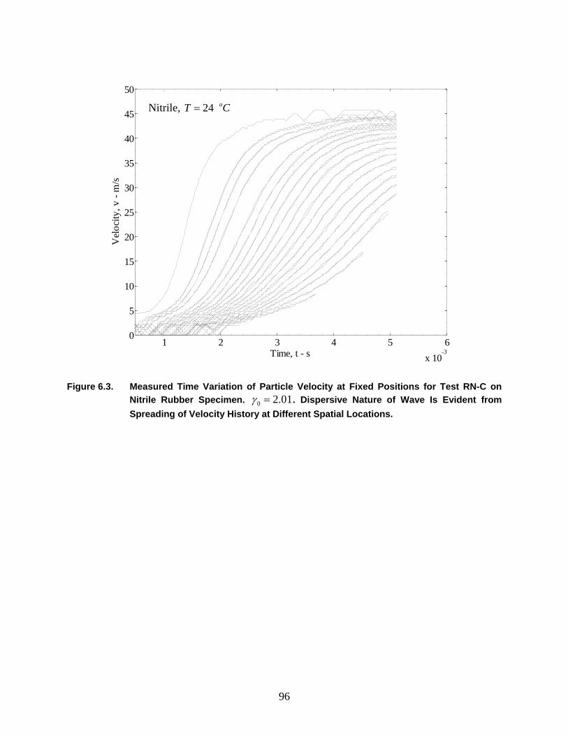
96

Figure 6.3. Measured Time Variation of Particle Velocity at Fixed Positions for Test RN-C on

Nitrile Rubber Specimen. 0 2.01γ = . Dispersive Nature of Wave Is Evident from Spreading of Velocity History at Different Spatial Locations.

1 2 3 4 5 6x 10

-3

0

5

10

15

20

25

30

35

40

45

50

Time, t - s

Vel

ocity

, v -

m/s

Nitrile, 24 oT C=

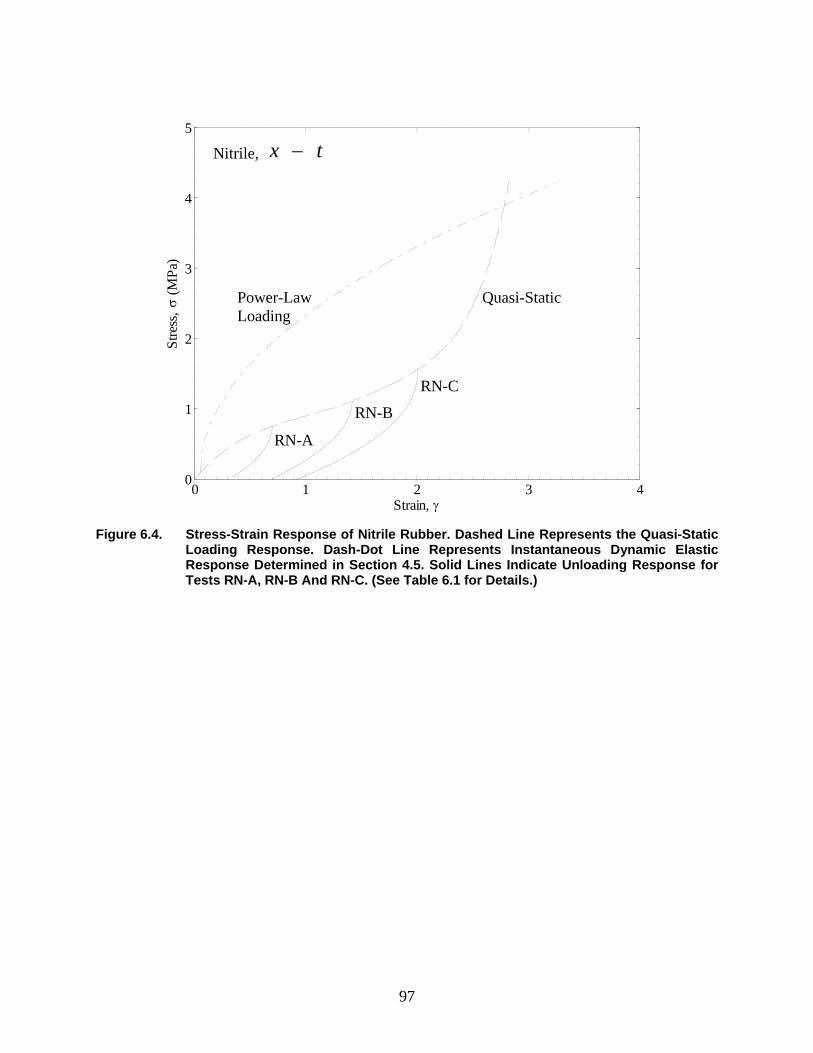
97

Figure 6.4. Stress-Strain Response of Nitrile Rubber. Dashed Line Represents the Quasi-Static

Loading Response. Dash-Dot Line Represents Instantaneous Dynamic Elastic Response Determined in Section 4.5. Solid Lines Indicate Unloading Response for Tests RN-A, RN-B And RN-C. (See Table 6.1 for Details.)

0 1 2 3 40

1

2

3

4

5

Strain, γ

Stre

ss, σ

(MPa

)Nitrile, x t−

Power-Law Loading

Quasi-Static

RN-C

RN-B

RN-A

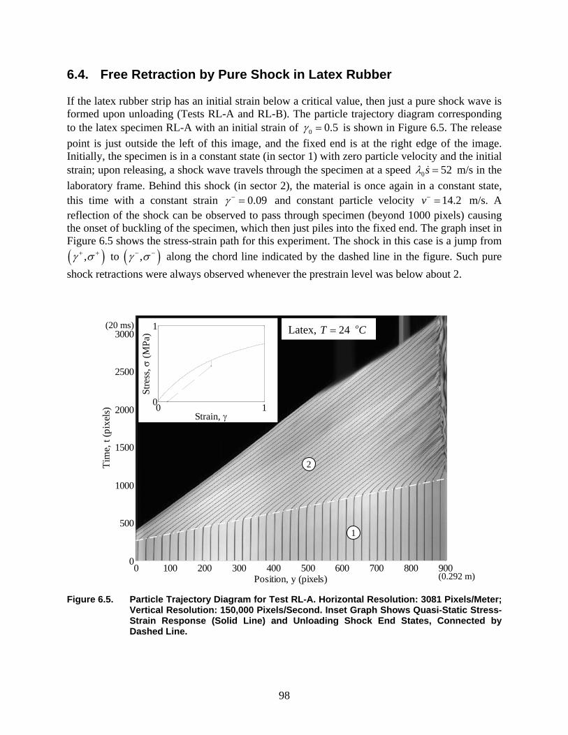
98

6.4. Free Retraction by Pure Shock in Latex Rubber If the latex rubber strip has an initial strain below a critical value, then just a pure shock wave is formed upon unloading (Tests RL-A and RL-B). The particle trajectory diagram corresponding to the latex specimen RL-A with an initial strain of 0 0.5γ = is shown in Figure 6.5. The release point is just outside the left of this image, and the fixed end is at the right edge of the image. Initially, the specimen is in a constant state (in sector 1) with zero particle velocity and the initial strain; upon releasing, a shock wave travels through the specimen at a speed 0 52sλ = m/s in the laboratory frame. Behind this shock (in sector 2), the material is once again in a constant state, this time with a constant strain 0.09γ − = and constant particle velocity 14.2v− = m/s. A reflection of the shock can be observed to pass through specimen (beyond 1000 pixels) causing the onset of buckling of the specimen, which then just piles into the fixed end. The graph inset in Figure 6.5 shows the stress-strain path for this experiment. The shock in this case is a jump from ( ),γ σ+ + to ( ),γ σ− − along the chord line indicated by the dashed line in the figure. Such pure shock retractions were always observed whenever the prestrain level was below about 2.

Figure 6.5. Particle Trajectory Diagram for Test RL-A. Horizontal Resolution: 3081 Pixels/Meter;

Vertical Resolution: 150,000 Pixels/Second. Inset Graph Shows Quasi-Static Stress-Strain Response (Solid Line) and Unloading Shock End States, Connected by Dashed Line.

0 100 200 300 400 500 600 700 800 9000

500

1000

1500

2000

2500

3000

Position, y (pixels)

Tim

e, t

(pix

els)

1

2

0 10

1

Strain, γ

Stre

ss, σ

(MPa

)

(0.292 m)

(20 ms) Latex, 24 oT C=

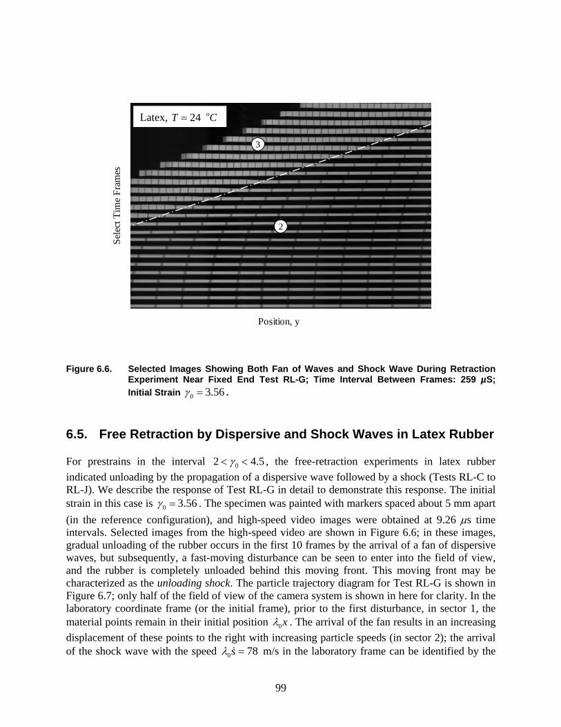
99

Figure 6.6. Selected Images Showing Both Fan of Waves and Shock Wave During Retraction

Experiment Near Fixed End Test RL-G; Time Interval Between Frames: 259 µS; Initial Strain 0 3.56γ = .

6.5. Free Retraction by Dispersive and Shock Waves in Latex Rubber For prestrains in the interval 02 4.5γ< < , the free-retraction experiments in latex rubber indicated unloading by the propagation of a dispersive wave followed by a shock (Tests RL-C to RL-J). We describe the response of Test RL-G in detail to demonstrate this response. The initial strain in this case is 0 3.56γ = . The specimen was painted with markers spaced about 5 mm apart (in the reference configuration), and high-speed video images were obtained at 9.26 µs time intervals. Selected images from the high-speed video are shown in Figure 6.6; in these images, gradual unloading of the rubber occurs in the first 10 frames by the arrival of a fan of dispersive waves, but subsequently, a fast-moving disturbance can be seen to enter into the field of view, and the rubber is completely unloaded behind this moving front. This moving front may be characterized as the unloading shock. The particle trajectory diagram for Test RL-G is shown in Figure 6.7; only half of the field of view of the camera system is shown in here for clarity. In the laboratory coordinate frame (or the initial frame), prior to the first disturbance, in sector 1, the material points remain in their initial position 0xλ . The arrival of the fan results in an increasing displacement of these points to the right with increasing particle speeds (in sector 2); the arrival of the shock wave with the speed 0 78sλ = m/s in the laboratory frame can be identified by the

Position, y

Sele

ct T

ime

Fram

esLatex, 24 oT C=

2

3

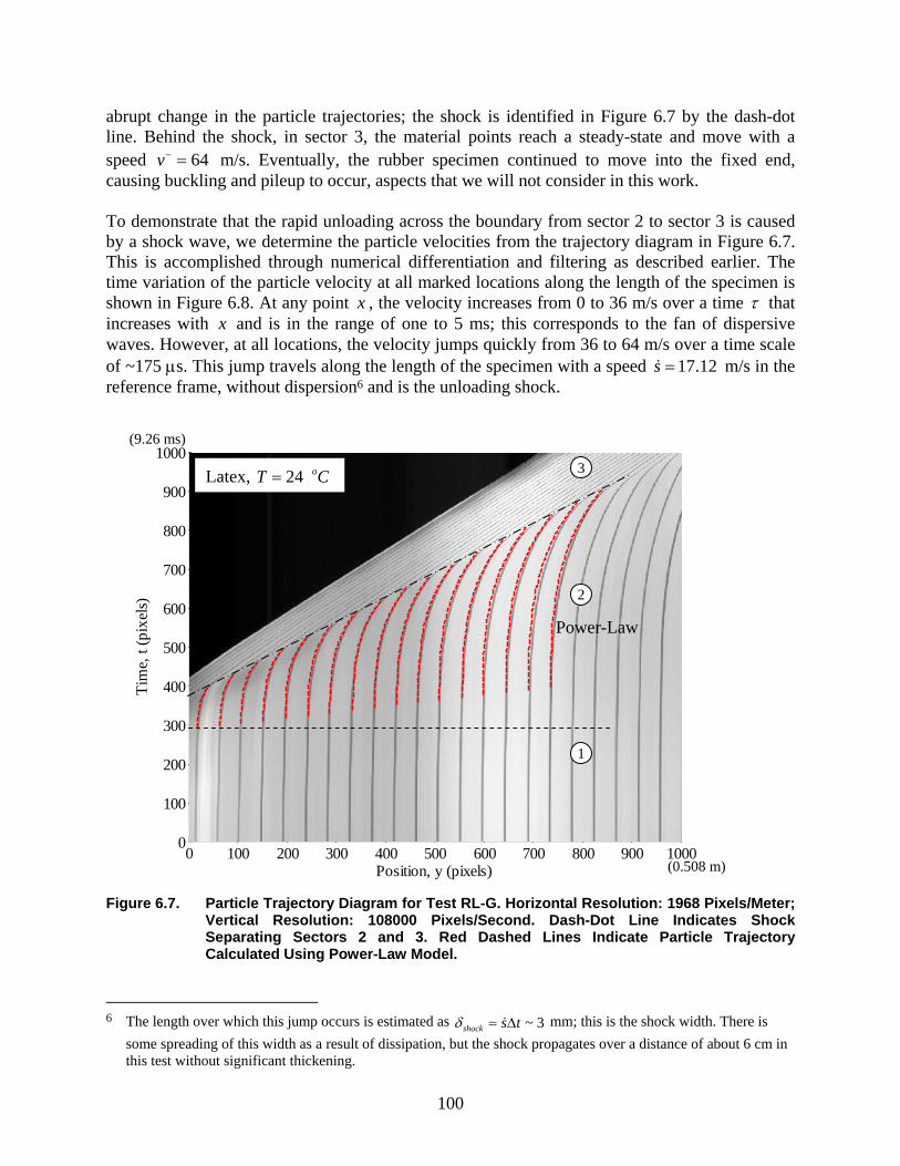
100

abrupt change in the particle trajectories; the shock is identified in Figure 6.7 by the dash-dot line. Behind the shock, in sector 3, the material points reach a steady-state and move with a speed 64v− = m/s. Eventually, the rubber specimen continued to move into the fixed end, causing buckling and pileup to occur, aspects that we will not consider in this work. To demonstrate that the rapid unloading across the boundary from sector 2 to sector 3 is caused by a shock wave, we determine the particle velocities from the trajectory diagram in Figure 6.7. This is accomplished through numerical differentiation and filtering as described earlier. The time variation of the particle velocity at all marked locations along the length of the specimen is shown in Figure 6.8. At any point x , the velocity increases from 0 to 36 m/s over a time τ that increases with x and is in the range of one to 5 ms; this corresponds to the fan of dispersive waves. However, at all locations, the velocity jumps quickly from 36 to 64 m/s over a time scale of ~175 µs. This jump travels along the length of the specimen with a speed 17.12s = m/s in the reference frame, without dispersion6 and is the unloading shock.

Figure 6.7. Particle Trajectory Diagram for Test RL-G. Horizontal Resolution: 1968 Pixels/Meter;

Vertical Resolution: 108000 Pixels/Second. Dash-Dot Line Indicates Shock Separating Sectors 2 and 3. Red Dashed Lines Indicate Particle Trajectory Calculated Using Power-Law Model.

6 The length over which this jump occurs is estimated as ~ 3shock s tδ = ∆ mm; this is the shock width. There is

some spreading of this width as a result of dissipation, but the shock propagates over a distance of about 6 cm in this test without significant thickening.

(9.26 ms)

0 100 200 300 400 500 600 700 800 900 10000

100

200

300

400

500

600

700

800

900

1000

Position, y (pixels)

Tim

e, t

(pix

els)

1

2

3

(0.508 m)

Latex, 24 oT C=

Power-Law

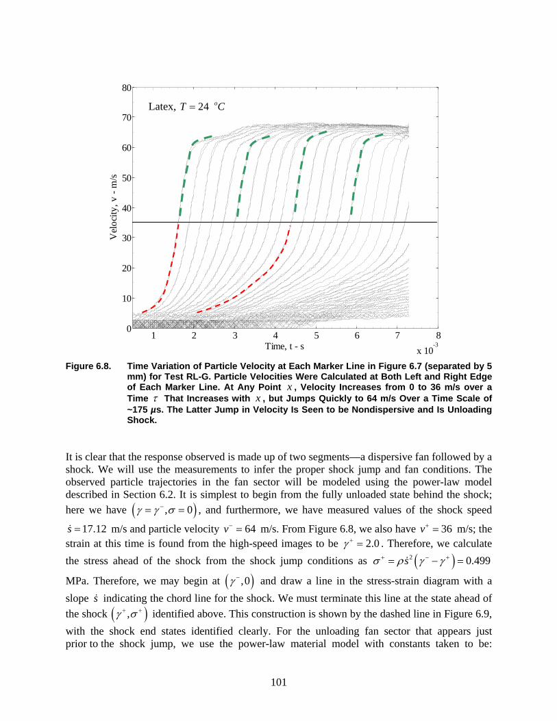
101

Figure 6.8. Time Variation of Particle Velocity at Each Marker Line in Figure 6.7 (separated by 5

mm) for Test RL-G. Particle Velocities Were Calculated at Both Left and Right Edge of Each Marker Line. At Any Point x , Velocity Increases from 0 to 36 m/s over a Time τ That Increases with x , but Jumps Quickly to 64 m/s Over a Time Scale of ~175 µs. The Latter Jump in Velocity Is Seen to be Nondispersive and Is Unloading Shock.

It is clear that the response observed is made up of two segments—a dispersive fan followed by a shock. We will use the measurements to infer the proper shock jump and fan conditions. The observed particle trajectories in the fan sector will be modeled using the power-law model described in Section 6.2. It is simplest to begin from the fully unloaded state behind the shock; here we have ( ), 0γ γ σ−= = , and furthermore, we have measured values of the shock speed

17.12s = m/s and particle velocity 64v− = m/s. From Figure 6.8, we also have 36v+ = m/s; the strain at this time is found from the high-speed images to be 2.0γ + = . Therefore, we calculate the stress ahead of the shock from the shock jump conditions as ( )2 0.499sσ ρ γ γ+ − += − =

MPa. Therefore, we may begin at ( ),0γ − and draw a line in the stress-strain diagram with a slope s indicating the chord line for the shock. We must terminate this line at the state ahead of the shock ( ),γ σ+ + identified above. This construction is shown by the dashed line in Figure 6.9, with the shock end states identified clearly. For the unloading fan sector that appears just prior to the shock jump, we use the power-law material model with constants taken to be:

1 2 3 4 5 6 7 8x 10

-3

0

10

20

30

40

50

60

70

80

Time, t - s

Vel

ocity

, v -

m/s

Latex, 24 oT C=

102

0.70rµ = MPa and 0.5rn = ; this choice was based on the ability to fit the particle trajectories prior to the formation of the shock. With this choice of parameters, Eq. (4-5) can be evaluated to obtain the particle trajectory until the onset of the shock; these trajectories are shown in Figure 6.7. The corresponding stress-strain diagram is indicated in Figure 6.9. Note that the quasi-static state corresponding to the prestrain is ( )0 , qsγ σ , with qsσ calculated using the quasi-static cubic model. The calculated response assembled from the shock and fan solution above does not quite reach up to qsσ at the initial state. Such discrepancy was not observed in the nitrile rubber and could point to an effect of kinetics associated with melting of strain-induced crystallites. The discrepancy could be for two reasons. First, there is some viscoelastic unloading in the rubber when stretched and held for a short duration before the free-retraction begins; we determined that this drop in stress is quite small since the hold time was under 30 s (Section 2.4). The second possibility is that under the rapid release conditions, the strain-induced crystallites that were formed during quasi-static loading do not have sufficient time for melting, and therefore, the stress unloads more rapidly than in the quasi-static case while the strain recovers very little, resulting in a nearly vertical drop in the stress-strain response. This requires further study, perhaps with instrumentation that can reveal such structural information. We note further that the initial stress 0σ does not appear in Eq. (4-5) and hence does not influence the fitting of the computed particle trajectories to the experimental trajectories. Therefore, we will take 0σ to be a free parameter and adjust it such that the stress calculated at the shock σ + matches the estimate obtained from the shock jump conditions; this value of 0σ is marked in Figure 6.9 by an asterisk. It is important to note that at the point of the shock jump, the power-law model is tangential to the shock line; this was not imposed but merely a consequence of obtaining a proper power-law material model that fits the dispersive wave regime. The observed tangency suggests that the criterion of maximum dissipation is automatically implied in the observed shock response. This also lends some credence to the process of using 0σ as a fitting parameter. This process is used to analyze all eight of the tests (Tests RL-C through RL-J); using an initial drop of the stress to

0σ , following this with a fan, calculated with a power-law hardening material model, and finally introducing the shock results in the stress-strain path for each of the tests as shown in Figure 6.10. The value of 0σ obtained in fitting each test is shown in Table 6.2; these appear to cluster around 1.3 MPa, the value that corresponds nearly to the onset of crystallization.

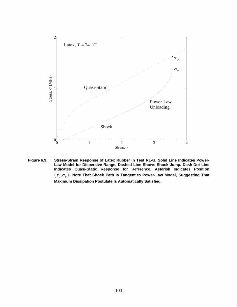
103

Figure 6.9. Stress-Strain Response of Latex Rubber in Test RL-G. Solid Line Indicates Power-

Law Model for Dispersive Range, Dashed Line Shows Shock Jump. Dash-Dot Line Indicates Quasi-Static Response for Reference. Asterisk Indicates Position ( )0 0,γ σ . Note That Shock Path Is Tangent to Power-Law Model, Suggesting That Maximum Dissipation Postulate Is Automatically Satisfied.

0 1 2 3 40

1

2

Strain, γ

Stre

ss, σ

(MPa

)Latex, 24 oT C=

Quasi-Static

Power-Law Unloading

Shock

0σ

qsσ

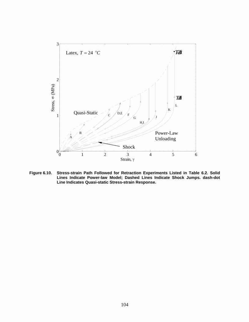
104

Figure 6.10. Stress-strain Path Followed for Retraction Experiments Listed in Table 6.2. Solid

Lines Indicate Power-law Model; Dashed Lines Indicate Shock Jumps. dash-dot Line Indicates Quasi-static Stress-strain Response.

0 1 2 3 4 5 60

1

2

3

Strain, γ

Stre

ss, σ

(MPa

)

A B

C D,E F G

H,I

J

K L

Quasi-Static

Latex, 24 oT C=

24oT C=

24oT C=

Power-Law Unloading

Shock

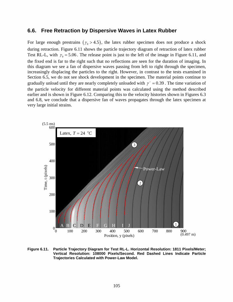
105

6.6. Free Retraction by Dispersive Waves in Latex Rubber For large enough prestrains ( )0 4.5γ > , the latex rubber specimen does not produce a shock during retraction. Figure 6.11 shows the particle trajectory diagram of retraction of latex rubber Test RL-L, with 0 5.06γ = . The release point is just to the left of the image in Figure 6.11, and the fixed end is far to the right such that no reflections are seen for the duration of imaging. In this diagram we see a fan of dispersive waves passing from left to right through the specimen, increasingly displacing the particles to the right. However, in contrast to the tests examined in Section 6.5, we do not see shock development in the specimen. The material points continue to gradually unload until they are nearly completely unloaded with 0.39γ − = . The time variation of the particle velocity for different material points was calculated using the method described earlier and is shown in Figure 6.12. Comparing this to the velocity histories shown in Figures 6.3 and 6.8, we conclude that a dispersive fan of waves propagates through the latex specimen at very large initial strains.

Figure 6.11. Particle Trajectory Diagram for Test RL-L. Horizontal Resolution: 1811 Pixels/Meter; Vertical Resolution: 108000 Pixels/Second. Red Dashed Lines Indicate Particle Trajectories Calculated with Power-Law Model.

0 100 200 300 400 500 600 700 800 9000

100

200

300

400

500

600

Position, y (pixels)

Tim

e, t

(pix

els)

(0.497 m)

(5.5 ms)

Latex, 24 oT C=

Power-Law

A B C E FD G H I J 1

2

3

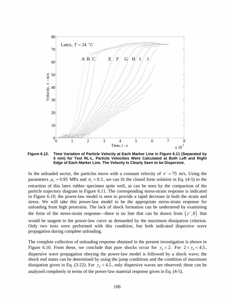
106

Figure 6.12. Time Variation of Particle Velocity at Each Marker Line in Figure 6.11 (Separated by

5 mm) for Test RL-L. Particle Velocities Were Calculated at Both Left and Right Edge of Each Marker Line. The Velocity Is Clearly Seen to be Dispersive.

In the unloaded sector, the particles move with a constant velocity of 75v− = m/s. Using the parameters 0.95rµ = MPa and 0.3rn = , we can fit the closed form solution in Eq. (4-5) to the retraction of this latex rubber specimen quite well, as can be seen by the comparison of the particle trajectory diagram in Figure 6.11. The corresponding stress-strain response is indicated in Figure 6.10; the power-law model is seen to provide a rapid decrease in both the strain and stress. We will take this power-law model to be the appropriate stress-strain response for unloading from high prestrains. The lack of shock formation can be understood by examining the form of the stress-strain response—there is no line that can be drawn from ( ),0γ − that would be tangent to the power-law curve as demanded by the maximum dissipation criterion. Only two tests were performed with this condition, but both indicated dispersive wave propagation during complete unloading. The complete collection of unloading response obtained in the present investigation is shown in Figure 6.10. From these, we conclude that pure shocks occur for 0 2γ < . For 02 4.5γ< < , dispersive wave propagation obeying the power-law model is followed by a shock wave; the shock end states can be determined by using the jump conditions and the condition of maximum dissipation given in Eq. (3-22). For 0 4.5γ > , only dispersive waves are observed; these can be analyzed completely in terms of the power-law material response given in Eq. (4-5).

0 1 2 3 4 5 6 7 8x 10

-3

0

10

20

30

40

50

60

70

80

Time, t - s

Vel

ocity

, v -

m/s

Latex, 24 oT C=

A B C E F G H I J

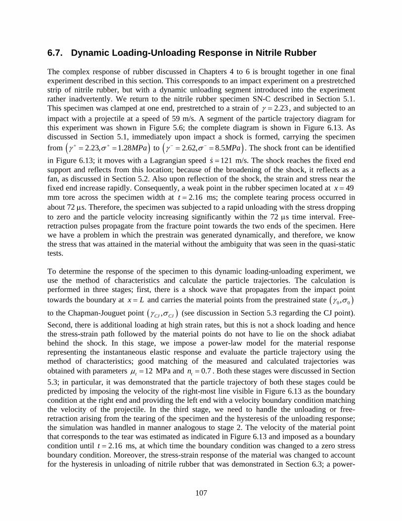
107

6.7. Dynamic Loading-Unloading Response in Nitrile Rubber The complex response of rubber discussed in Chapters 4 to 6 is brought together in one final experiment described in this section. This corresponds to an impact experiment on a prestretched strip of nitrile rubber, but with a dynamic unloading segment introduced into the experiment rather inadvertently. We return to the nitrile rubber specimen SN-C described in Section 5.1. This specimen was clamped at one end, prestretched to a strain of 2.23γ = , and subjected to an impact with a projectile at a speed of 59 m/s. A segment of the particle trajectory diagram for this experiment was shown in Figure 5.6; the complete diagram is shown in Figure 6.13. As discussed in Section 5.1, immediately upon impact a shock is formed, carrying the specimen from ( )2.23, 1.28MPaγ σ+ += = to ( )2.62, 8.5MPaγ σ− −= = . The shock front can be identified in Figure 6.13; it moves with a Lagrangian speed 121s = m/s. The shock reaches the fixed end support and reflects from this location; because of the broadening of the shock, it reflects as a fan, as discussed in Section 5.2. Also upon reflection of the shock, the strain and stress near the fixed end increase rapidly. Consequently, a weak point in the rubber specimen located at 49x = mm tore across the specimen width at 2.16t = ms; the complete tearing process occurred in about 72 µs. Therefore, the specimen was subjected to a rapid unloading with the stress dropping to zero and the particle velocity increasing significantly within the 72 µs time interval. Free-retraction pulses propagate from the fracture point towards the two ends of the specimen. Here we have a problem in which the prestrain was generated dynamically, and therefore, we know the stress that was attained in the material without the ambiguity that was seen in the quasi-static tests. To determine the response of the specimen to this dynamic loading-unloading experiment, we use the method of characteristics and calculate the particle trajectories. The calculation is performed in three stages; first, there is a shock wave that propagates from the impact point towards the boundary at x L= and carries the material points from the prestrained state ( )0 0,γ σ

to the Chapman-Jouguet point ( ),CJ CJγ σ (see discussion in Section 5.3 regarding the CJ point). Second, there is additional loading at high strain rates, but this is not a shock loading and hence the stress-strain path followed by the material points do not have to lie on the shock adiabat behind the shock. In this stage, we impose a power-law model for the material response representing the instantaneous elastic response and evaluate the particle trajectory using the method of characteristics; good matching of the measured and calculated trajectories was obtained with parameters 12tµ = MPa and 0.7tn = . Both these stages were discussed in Section 5.3; in particular, it was demonstrated that the particle trajectory of both these stages could be predicted by imposing the velocity of the right-most line visible in Figure 6.13 as the boundary condition at the right end and providing the left end with a velocity boundary condition matching the velocity of the projectile. In the third stage, we need to handle the unloading or free-retraction arising from the tearing of the specimen and the hysteresis of the unloading response; the simulation was handled in manner analogous to stage 2. The velocity of the material point that corresponds to the tear was estimated as indicated in Figure 6.13 and imposed as a boundary condition until 2.16t = ms, at which time the boundary condition was changed to a zero stress boundary condition. Moreover, the stress-strain response of the material was changed to account for the hysteresis in unloading of nitrile rubber that was demonstrated in Section 6.3; a power-

108

law model was again used for the unloading response with 35rµ = MPa and 0.85rn = ; the corresponding stress-strain response is shown in Figure 6.14. The material constants were obtained by matching the observed particle trajectories in this stage. The calculated particle trajectories match the observed free-retraction quite well for a short duration (see Figure 6.13). The success of this simulation in reproducing dynamic unloading suggests that the power-law model proposed in Eq. (4-1) for the unloading response is suitable for capturing the hysteretic behavior of rubbers.

Figure 6.13. Particle Trajectory Diagram for Test SN-C. Horizontal Resolution: 3347 Pixels/Meter;

Vertical Resolution: 250000 Pixels/Second. Red Dashed Lines Indicate Trajectories Calculated with the Power-Law Model. The Label T Identifies Location Where the Specimen Ruptured.

0 50 100 150 200 250 300 350 400 4500

100

200

300

400

500

600

Position, y (pixels)

Tim

e, t

(pix

els)

T

(0.134 m)

(2.4 ms) Nitrile, 0σ

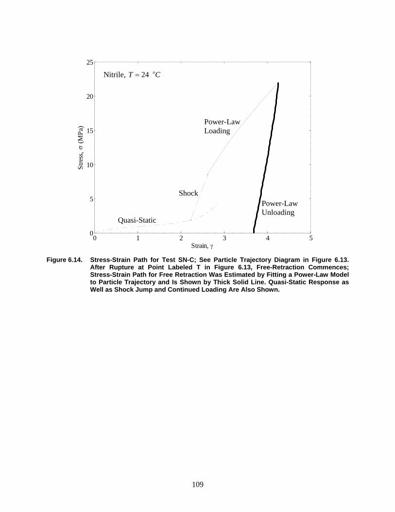
109

Figure 6.14. Stress-Strain Path for Test SN-C; See Particle Trajectory Diagram in Figure 6.13. After Rupture at Point Labeled T in Figure 6.13, Free-Retraction Commences; Stress-Strain Path for Free Retraction Was Estimated by Fitting a Power-Law Model to Particle Trajectory and Is Shown by Thick Solid Line. Quasi-Static Response as Well as Shock Jump and Continued Loading Are Also Shown.

0 1 2 3 4 50

5

10

15

20

25

Strain, γ

Stre

ss, σ

(MPa

)Nitrile, 24 oT C=

Quasi-Static

Shock

Power-Law Loading

Power-Law Unloading

110

7. KOLSKY EXPERIMENT 7.1. Experimental Setup At this point we introduce the last experiment conducted on the thin strips of rubber. This is a variant of an experiment that was first used by Kolsky to explore shock waves. Kolsky (1969) stretched a rubber bar to a large initial strain and clamped the two ends rigidly. Subsequently, one segment of this strip was subjected to a further increase in strain such that the highly strained region had a strain of around 4.4 and the neighboring region had a strain of 4; upon releasing the constraint in the middle, the high-strain level propagated into the low-strain region, while an unloading propagated to the high-strain region. By measuring the particle velocity in the low-strain region with an electromagnetic system, Kolsky demonstrated that a shock wave develops at some large distance from the original release point. Our interest in the Kolsky experiment is motivated not by the exploration of shock waves (these have been explored both in impact and retraction experiments in Chapters 5 and 6 respectively), but in exploring the effects of hysteretic material behavior wave propagation; this experiment brings together both dispersive wave propagation and hysteretic behavior. In this experiment, we take a strip of rubber of length, L, and stretch to desired length, ( )1o Lγ + . Subsequently, both ends are fixed to maintain this length throughout this experiment. A segment of the specimen of length ξ is stretched further, thereby producing two different strains in the specimen: a high strain region (HSR) with ( ) 1xγ γ= for 0 x ξ< < , and a low strain region

(LSR) with ( ) 2xγ γ= for x Lξ < < . This is illustrated in Figure 7.1. In practice, the different strains in the two regions are maintained initially by a holding clamp consisting of two parallel rollers that pinch the specimen along the width when squeezed by between two fingers. These rollers travel along guiding rails and are spring loaded such that upon release of finger pressure, the rollers separate and release the constraint on the specimen. It is expected that a fan of tensile loading waves travels into the LSR and a corresponding fan of tensile unloading waves travels into the HSR. Markers were drawn across the width of the specimen at 5 mm intervals along the entire length of the specimen in order to track the particle trajectories. These markers were imaged by a Photron SA1.1 high-speed video camera at a rate of 150,000 frames per second for about 300 ms. The force exerted by the specimen at the restraining ends was measured with two piezoelectric force sensors, (PCB Piezotronics Model 208C01); these sensors were placed between the grips holding the specimen and the rigid fixture.

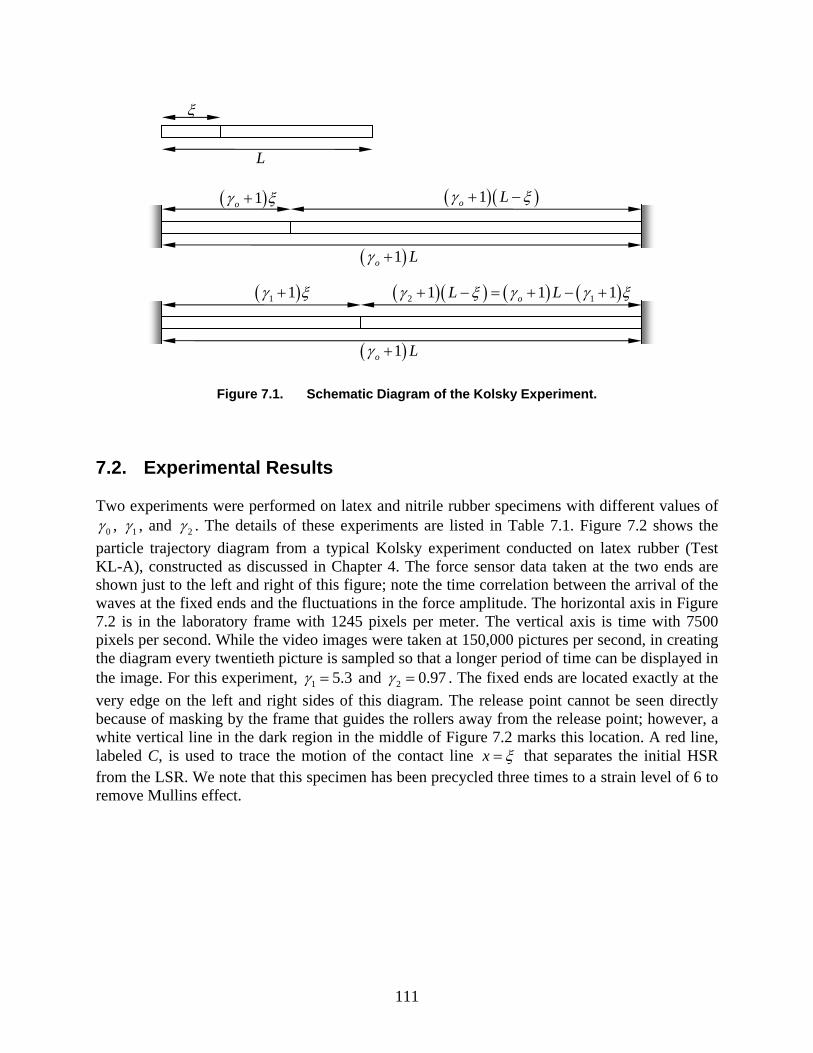
111

Figure 7.1. Schematic Diagram of the Kolsky Experiment. 7.2. Experimental Results Two experiments were performed on latex and nitrile rubber specimens with different values of

0γ , 1γ , and 2γ . The details of these experiments are listed in Table 7.1. Figure 7.2 shows the particle trajectory diagram from a typical Kolsky experiment conducted on latex rubber (Test KL-A), constructed as discussed in Chapter 4. The force sensor data taken at the two ends are shown just to the left and right of this figure; note the time correlation between the arrival of the waves at the fixed ends and the fluctuations in the force amplitude. The horizontal axis in Figure 7.2 is in the laboratory frame with 1245 pixels per meter. The vertical axis is time with 7500 pixels per second. While the video images were taken at 150,000 pictures per second, in creating the diagram every twentieth picture is sampled so that a longer period of time can be displayed in the image. For this experiment, 1 5.3γ = and 2 0.97γ = . The fixed ends are located exactly at the very edge on the left and right sides of this diagram. The release point cannot be seen directly because of masking by the frame that guides the rollers away from the release point; however, a white vertical line in the dark region in the middle of Figure 7.2 marks this location. A red line, labeled C, is used to trace the motion of the contact line x ξ= that separates the initial HSR from the LSR. We note that this specimen has been precycled three times to a strain level of 6 to remove Mullins effect.

ξ

L

( )1oγ ξ+ ( )( )1o Lγ ξ+ −

( )1o Lγ +

( )1o Lγ +

( )1 1γ ξ+ ( )( ) ( ) ( )2 11 1 1oL Lγ ξ γ γ ξ+ − = + − +

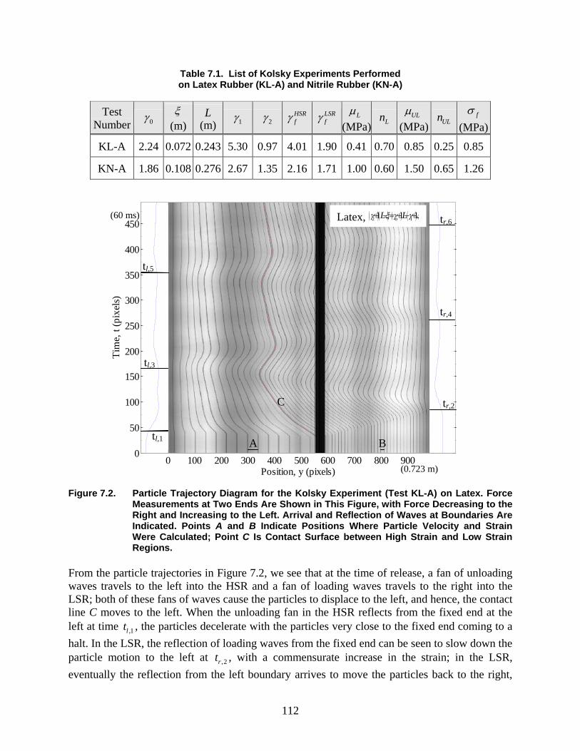
112

Table 7.1. List of Kolsky Experiments Performed on Latex Rubber (KL-A) and Nitrile Rubber (KN-A)

Test Number 0γ ξ

(m) L

(m) 1γ 2γ HSRfγ LSR

fγ Lµ (MPa) Ln ULµ

(MPa) ULn fσ (MPa)

KL-A 2.24 0.072 0.243 5.30 0.97 4.01 1.90 0.41 0.70 0.85 0.25 0.85

KN-A 1.86 0.108 0.276 2.67 1.35 2.16 1.71 1.00 0.60 1.50 0.65 1.26

Figure 7.2. Particle Trajectory Diagram for the Kolsky Experiment (Test KL-A) on Latex. Force

Measurements at Two Ends Are Shown in This Figure, with Force Decreasing to the Right and Increasing to the Left. Arrival and Reflection of Waves at Boundaries Are Indicated. Points A and B Indicate Positions Where Particle Velocity and Strain Were Calculated; Point C Is Contact Surface between High Strain and Low Strain Regions.

From the particle trajectories in Figure 7.2, we see that at the time of release, a fan of unloading waves travels to the left into the HSR and a fan of loading waves travels to the right into the LSR; both of these fans of waves cause the particles to displace to the left, and hence, the contact line C moves to the left. When the unloading fan in the HSR reflects from the fixed end at the left at time ,1lt , the particles decelerate with the particles very close to the fixed end coming to a halt. In the LSR, the reflection of loading waves from the fixed end can be seen to slow down the particle motion to the left at ,2rt , with a commensurate increase in the strain; in the LSR, eventually the reflection from the left boundary arrives to move the particles back to the right,

0 100 200 300 400 500 600 700 800 9000

50

100

150

200

250

300

350

400

450

Position, y (pixels)

Tim

e, t

(pix

els)

(0.723 m)

(60 ms)

A

C

Btl,1

tl,3

tl,5

tr,2

tr,4

tr,6 Latex, ( )( ) ( ) ( )2 11 1 1oL Lγ ξ γ γ ξ+ − = + − +

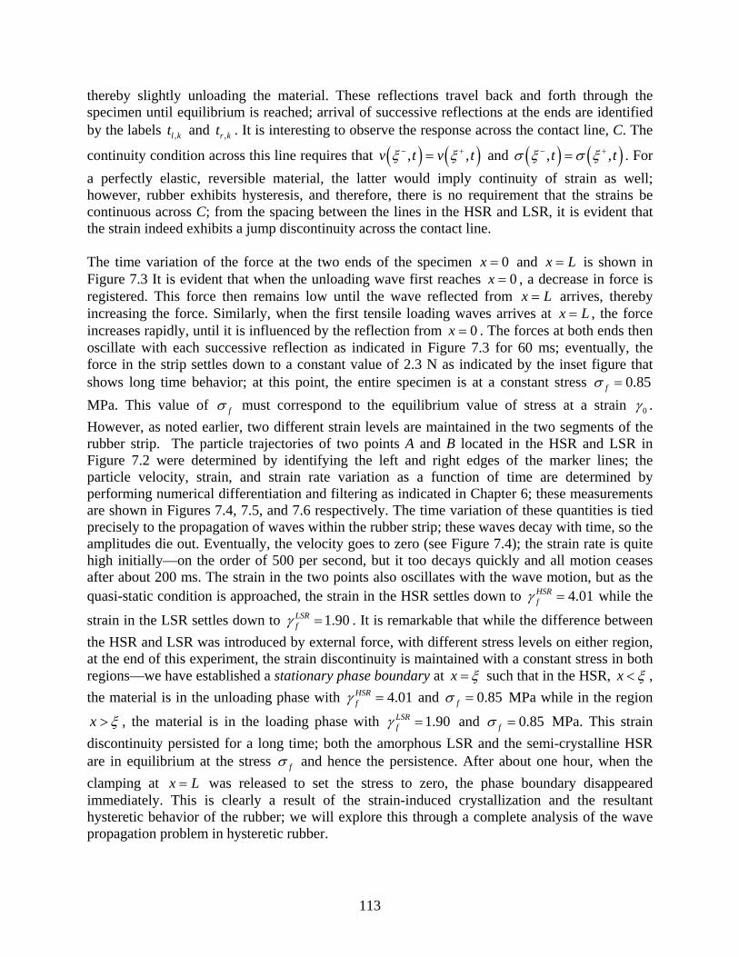
113

thereby slightly unloading the material. These reflections travel back and forth through the specimen until equilibrium is reached; arrival of successive reflections at the ends are identified by the labels ,l kt and ,r kt . It is interesting to observe the response across the contact line, C. The

continuity condition across this line requires that ( ) ( ), ,v t v tξ ξ− += and ( ) ( ), ,t tσ ξ σ ξ− += . For a perfectly elastic, reversible material, the latter would imply continuity of strain as well; however, rubber exhibits hysteresis, and therefore, there is no requirement that the strains be continuous across C; from the spacing between the lines in the HSR and LSR, it is evident that the strain indeed exhibits a jump discontinuity across the contact line. The time variation of the force at the two ends of the specimen 0x = and x L= is shown in Figure 7.3 It is evident that when the unloading wave first reaches 0x = , a decrease in force is registered. This force then remains low until the wave reflected from x L= arrives, thereby increasing the force. Similarly, when the first tensile loading waves arrives at x L= , the force increases rapidly, until it is influenced by the reflection from 0x = . The forces at both ends then oscillate with each successive reflection as indicated in Figure 7.3 for 60 ms; eventually, the force in the strip settles down to a constant value of 2.3 N as indicated by the inset figure that shows long time behavior; at this point, the entire specimen is at a constant stress 0.85fσ = MPa. This value of fσ must correspond to the equilibrium value of stress at a strain 0γ . However, as noted earlier, two different strain levels are maintained in the two segments of the rubber strip. The particle trajectories of two points A and B located in the HSR and LSR in Figure 7.2 were determined by identifying the left and right edges of the marker lines; the particle velocity, strain, and strain rate variation as a function of time are determined by performing numerical differentiation and filtering as indicated in Chapter 6; these measurements are shown in Figures 7.4, 7.5, and 7.6 respectively. The time variation of these quantities is tied precisely to the propagation of waves within the rubber strip; these waves decay with time, so the amplitudes die out. Eventually, the velocity goes to zero (see Figure 7.4); the strain rate is quite high initially—on the order of 500 per second, but it too decays quickly and all motion ceases after about 200 ms. The strain in the two points also oscillates with the wave motion, but as the quasi-static condition is approached, the strain in the HSR settles down to 4.01HSR

fγ = while the

strain in the LSR settles down to 1.90LSRfγ = . It is remarkable that while the difference between

the HSR and LSR was introduced by external force, with different stress levels on either region, at the end of this experiment, the strain discontinuity is maintained with a constant stress in both regions—we have established a stationary phase boundary at x ξ= such that in the HSR, x ξ< , the material is in the unloading phase with 4.01HSR

fγ = and 0.85fσ = MPa while in the region

x ξ> , the material is in the loading phase with 1.90LSRfγ = and 0.85fσ = MPa. This strain

discontinuity persisted for a long time; both the amorphous LSR and the semi-crystalline HSR are in equilibrium at the stress fσ and hence the persistence. After about one hour, when the clamping at x L= was released to set the stress to zero, the phase boundary disappeared immediately. This is clearly a result of the strain-induced crystallization and the resultant hysteretic behavior of the rubber; we will explore this through a complete analysis of the wave propagation problem in hysteretic rubber.

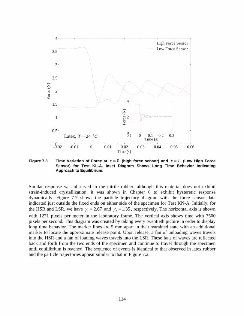
114

Figure 7.3. Time Variation of Force at 0x = (high force sensor) and x L= (Low High Force

Sensor) for Test KL-A. Inset Diagram Shows Long Time Behavior Indicating Approach to Equilibrium.

Similar response was observed in the nitrile rubber; although this material does not exhibit strain-induced crystallization, it was shown in Chapter 6 to exhibit hysteretic response dynamically. Figure 7.7 shows the particle trajectory diagram with the force sensor data indicated just outside the fixed ends on either side of the specimen for Test KN-A. Initially, for the HSR and LSR, we have 1 2.67γ = and 2 1.35γ = , respectively. The horizontal axis is shown with 1271 pixels per meter in the laboratory frame. The vertical axis shows time with 7500 pixels per second. This diagram was created by taking every twentieth picture in order to display long time behavior. The marker lines are 5 mm apart in the unstrained state with an additional marker to locate the approximate release point. Upon release, a fan of unloading waves travels into the HSR and a fan of loading waves travels into the LSR. These fans of waves are reflected back and forth from the two ends of the specimen and continue to travel through the specimen until equilibrium is reached. The sequence of events is identical to that observed in latex rubber and the particle trajectories appear similar to that in Figure 7.2.

-0.02 -0.01 0 0.01 0.02 0.03 0.04 0.05 0.060

0.5

1

1.5

2

2.5

3

3.5

4

Time (s)

Forc

e (N

)

High Force SensorLow Force Sensor

-0.1 0 0.1 0.2 0.30

2

4

Time (s)

Forc

e (N

)

Latex, 24 oT C=

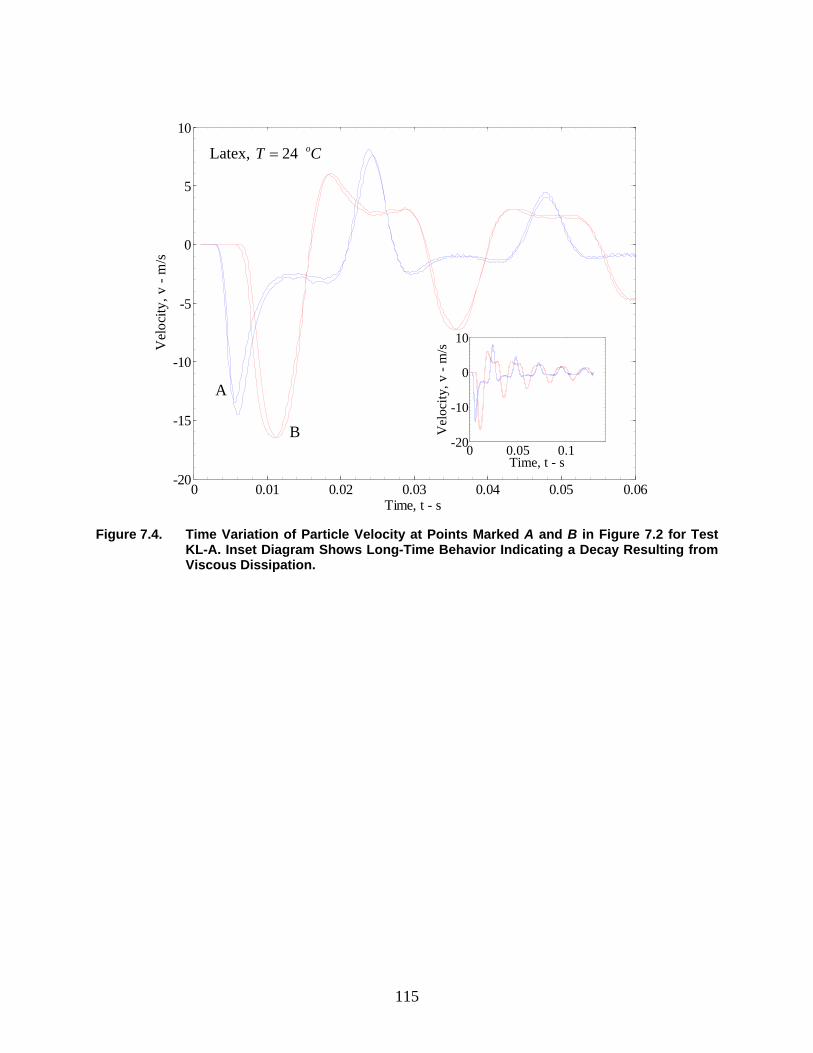
115

Figure 7.4. Time Variation of Particle Velocity at Points Marked A and B in Figure 7.2 for Test

KL-A. Inset Diagram Shows Long-Time Behavior Indicating a Decay Resulting from Viscous Dissipation.

0 0.01 0.02 0.03 0.04 0.05 0.06-20

-15

-10

-5

0

5

10

Time, t - s

Vel

ocity

, v -

m/s

0 0.05 0.1-20

-10

0

10

Time, t - sV

eloc

ity, v

- m

/sB

A

Latex, 24 oT C=

116

Figure 7.5. Time Variation of the Strain at Points Marked A and B in Figure 7.2, for Test KL-A.

Inset Diagram Shows the Long Time Behavior Indicating that the LSR and HSR Settle Down to Different Strain Levels with a Jump Across the Contact Line C.

0 0.01 0.02 0.03 0.04 0.05 0.060

1

2

3

4

5

6

Time, t - s

Stra

in, γ

A

B 0 0.05 0.10

5

10

Time, t - s

Stra

in, γ

Latex, 24 oT C=

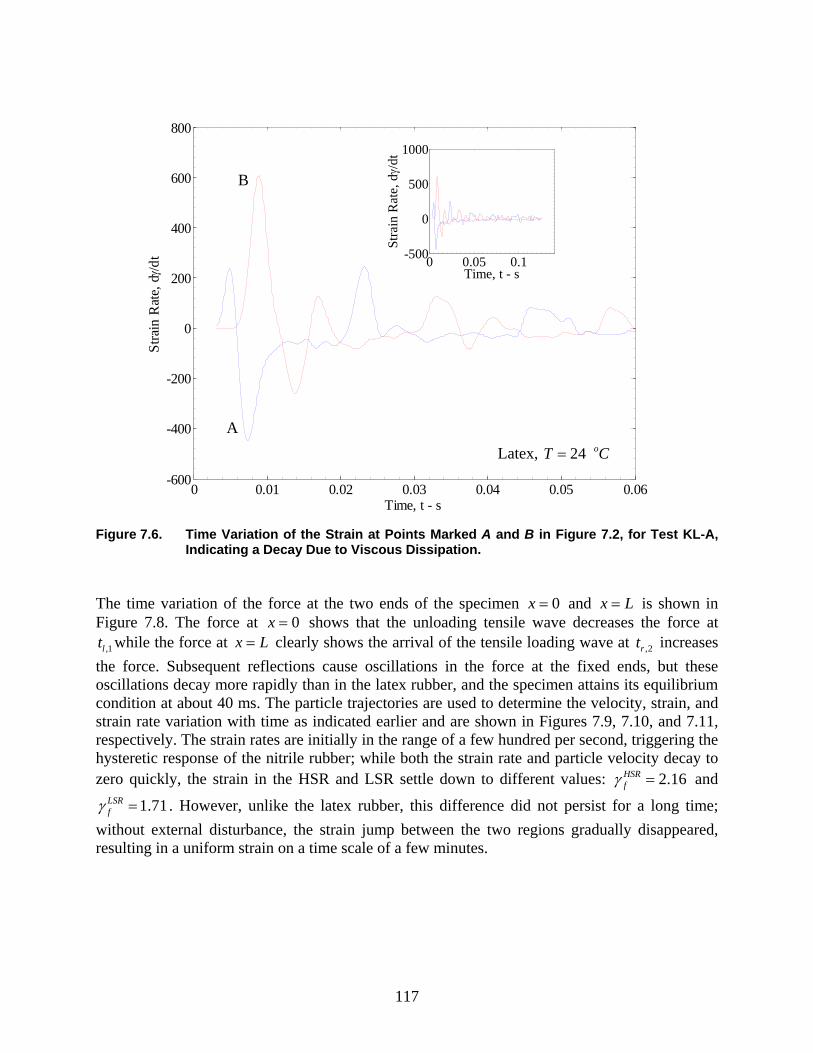
117

Figure 7.6. Time Variation of the Strain at Points Marked A and B in Figure 7.2, for Test KL-A,

Indicating a Decay Due to Viscous Dissipation. The time variation of the force at the two ends of the specimen 0x = and x L= is shown in Figure 7.8. The force at 0x = shows that the unloading tensile wave decreases the force at

,1lt while the force at x L= clearly shows the arrival of the tensile loading wave at ,2rt increases the force. Subsequent reflections cause oscillations in the force at the fixed ends, but these oscillations decay more rapidly than in the latex rubber, and the specimen attains its equilibrium condition at about 40 ms. The particle trajectories are used to determine the velocity, strain, and strain rate variation with time as indicated earlier and are shown in Figures 7.9, 7.10, and 7.11, respectively. The strain rates are initially in the range of a few hundred per second, triggering the hysteretic response of the nitrile rubber; while both the strain rate and particle velocity decay to zero quickly, the strain in the HSR and LSR settle down to different values: 2.16HSR

fγ = and

1.71LSRfγ = . However, unlike the latex rubber, this difference did not persist for a long time;

without external disturbance, the strain jump between the two regions gradually disappeared, resulting in a uniform strain on a time scale of a few minutes.

0 0.01 0.02 0.03 0.04 0.05 0.06-600

-400

-200

0

200

400

600

800

Time, t - s

Stra

in R

ate,

dγ /d

t

B

A

0 0.05 0.1-500

0

500

1000

Time, t - s

Stra

in R

ate,

dγ /

dt

Latex, 24 oT C=

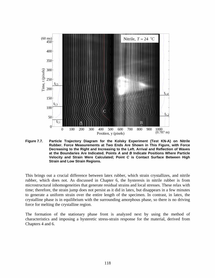
118

Figure 7.7. Particle Trajectory Diagram for the Kolsky Experiment (Test KN-A) on Nitrile Rubber. Force Measurements at Two Ends Are Shown in This Figure, with Force Decreasing to the Right and Increasing to the Left. Arrival and Reflection of Waves at the Boundaries Are Indicated. Points A and B Indicate Positions Where Particle Velocity and Strain Were Calculated; Point C is Contact Surface Between High Strain and Low Strain Regions.

This brings out a crucial difference between latex rubber, which strain crystallizes, and nitrile rubber, which does not. As discussed in Chapter 6, the hysteresis in nitrile rubber is from microstructural inhomogeneities that generate residual strains and local stresses. These relax with time; therefore, the strain jump does not persist as it did in latex, but disappears in a few minutes to generate a uniform strain over the entire length of the specimen. In contrast, in latex, the crystalline phase is in equilibrium with the surrounding amorphous phase, so there is no driving force for melting the crystalline region. The formation of the stationary phase front is analyzed next by using the method of characteristics and imposing a hysteretic stress-strain response for the material, derived from Chapters 4 and 6.

0 100 200 300 400 500 600 700 800 900 10000

50

100

150

200

250

300

350

400

450

Position, y (pixels)

Tim

e, t

(pix

els)

(0.787 m)

(60 ms)

A

C

Btl,1

tl,3

tl,5

tr,2

tr,4

Nitrile, 24 oT C=

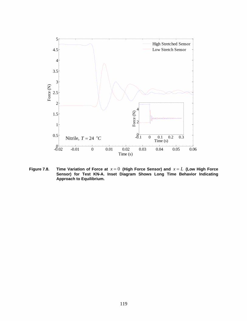
119

Figure 7.8. Time Variation of Force at 0x = (High Force Sensor) and x L= (Low High Force

Sensor) for Test KN-A. Inset Diagram Shows Long Time Behavior Indicating Approach to Equilibrium.

-0.02 -0.01 0 0.01 0.02 0.03 0.04 0.05 0.060

0.5

1

1.5

2

2.5

3

3.5

4

4.5

5

Time (s)

Forc

e (N

)

High Stretched SensorLow Stretch Sensor

-0.1 0 0.1 0.2 0.30

2

4

Time (s)Fo

rce

(N)

Nitrile, 24 oT C=

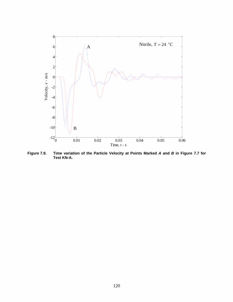
120

Figure 7.9. Time variation of the Particle Velocity at Points Marked A and B in Figure 7.7 for Test KN-A.

0 0.01 0.02 0.03 0.04 0.05 0.06-12

-10

-8

-6

-4

-2

0

2

4

6

8

Time, t - s

Vel

ocity

, v -

m/s

B

A Nitrile, 24 oT C=

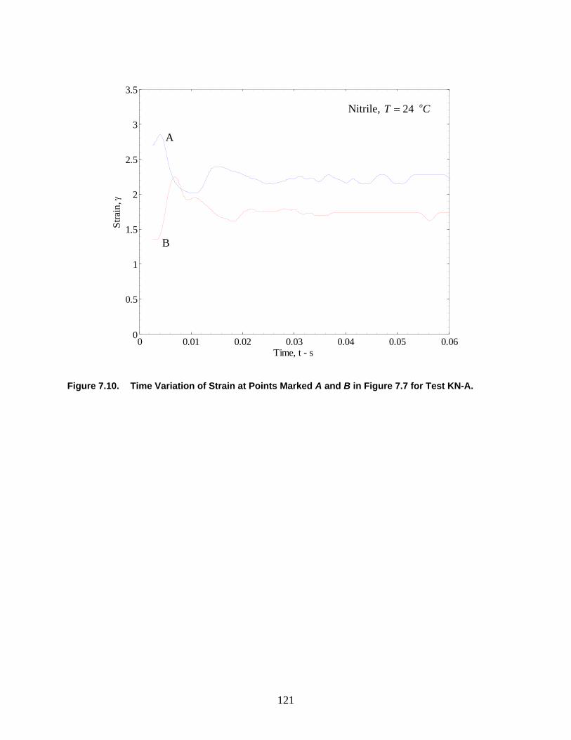
121

Figure 7.10. Time Variation of Strain at Points Marked A and B in Figure 7.7 for Test KN-A.

0 0.01 0.02 0.03 0.04 0.05 0.060

0.5

1

1.5

2

2.5

3

3.5

Time, t - s

Stra

in, γ

A

B

Nitrile, 24 oT C=

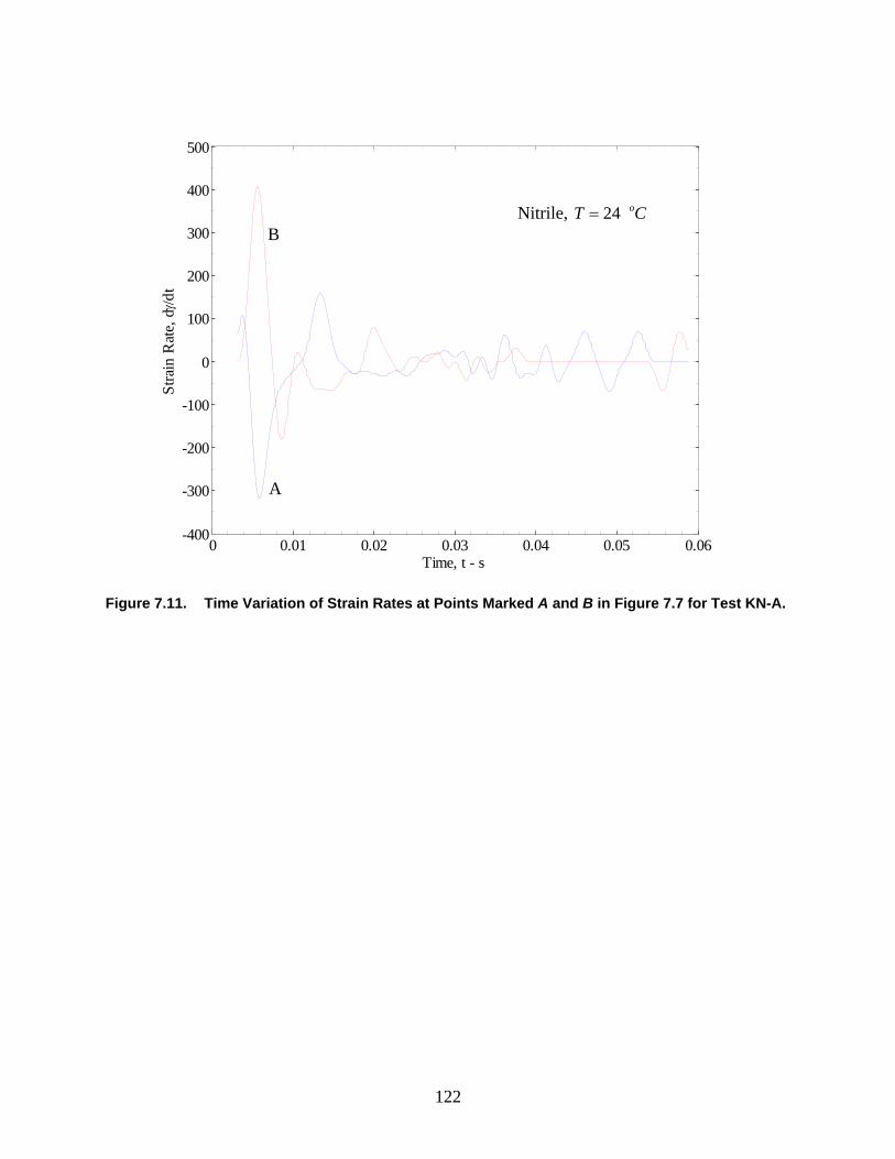
122

Figure 7.11. Time Variation of Strain Rates at Points Marked A and B in Figure 7.7 for Test KN-A.

0 0.01 0.02 0.03 0.04 0.05 0.06-400

-300

-200

-100

0

100

200

300

400

500

Time, t - s

Stra

in R

ate,

dγ /d

t

A

B Nitrile, 24 oT C=

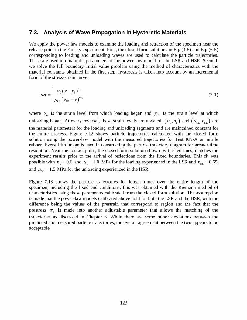
123

7.3. Analysis of Wave Propagation in Hysteretic Materials We apply the power law models to examine the loading and retraction of the specimen near the release point in the Kolsky experiment. First, the closed form solutions in Eq. (4-5) and Eq. (6-5) corresponding to loading and unloading waves are used to calculate the particle trajectories. These are used to obtain the parameters of the power-law model for the LSR and HSR. Second, we solve the full boundary-initial value problem using the method of characteristics with the material constants obtained in the first step; hysteresis is taken into account by an incremental form of the stress-strain curve:

( )( )

L

UL

nL L

nUL UL

dµ γ γ

σµ γ γ

⎧ −⎪= ⎨−⎪⎩

, (7-1)

where Lγ is the strain level from which loading began and ULγ is the strain level at which unloading began. At every reversal, these strain levels are updated. ( ),L Lnµ and ( ),UL ULnµ are the material parameters for the loading and unloading segments and are maintained constant for the entire process. Figure 7.12 shows particle trajectories calculated with the closed form solution using the power-law model with the measured trajectories for Test KN-A on nitrile rubber. Every fifth image is used in constructing the particle trajectory diagram for greater time resolution. Near the contact point, the closed form solution shown by the red lines, matches the experiment results prior to the arrival of reflections from the fixed boundaries. This fit was possible with 0.6Ln = and 1.0Lµ = MPa for the loading experienced in the LSR and 0.65ULn = and 1.5ULµ = MPa for the unloading experienced in the HSR. Figure 7.13 shows the particle trajectories for longer times over the entire length of the specimen, including the fixed end conditions; this was obtained with the Riemann method of characteristics using these parameters calibrated from the closed form solution. The assumption is made that the power-law models calibrated above hold for both the LSR and the HSR, with the difference being the values of the prestrain that correspond to region and the fact that the prestress 0σ is made into another adjustable parameter that allows the matching of the trajectories as discussed in Chapter 6. While there are some minor deviations between the predicted and measured particle trajectories, the overall agreement between the two appears to be acceptable.

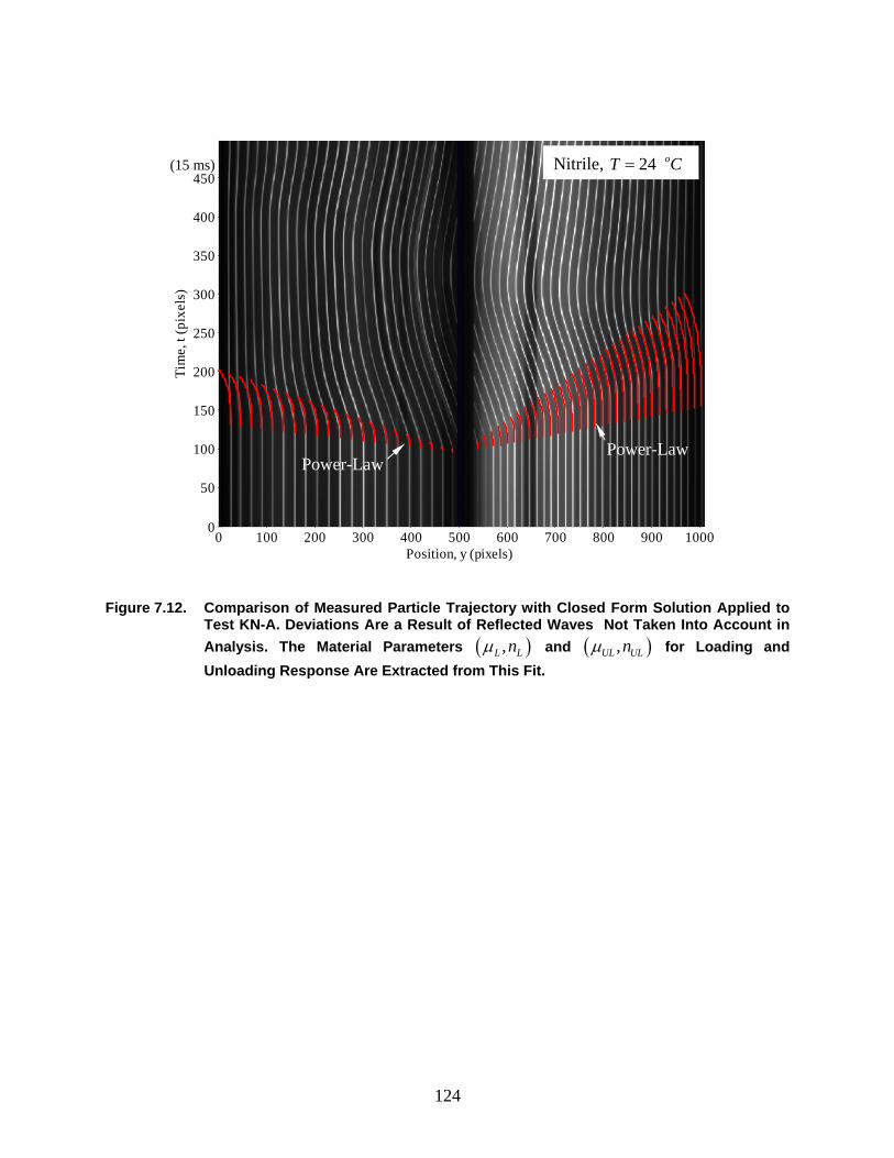
124

Figure 7.12. Comparison of Measured Particle Trajectory with Closed Form Solution Applied to Test KN-A. Deviations Are a Result of Reflected Waves Not Taken Into Account in Analysis. The Material Parameters ( ),L Lnµ and ( ),UL ULnµ for Loading and Unloading Response Are Extracted from This Fit.

(15 ms)

0 100 200 300 400 500 600 700 800 900 10000

50

100

150

200

250

300

350

400

450

Position, y (pixels)

Tim

e, t

(pix

els)

Nitrile, 24 oT C=

Power-LawPower-Law

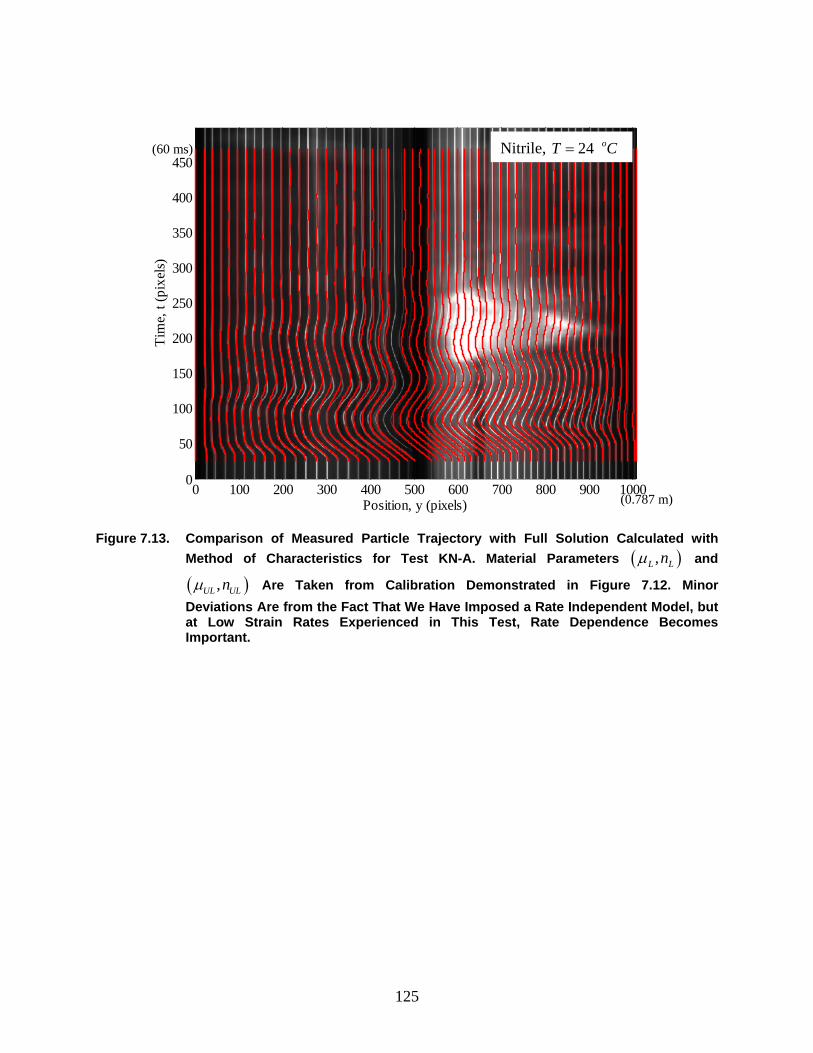
125

Figure 7.13. Comparison of Measured Particle Trajectory with Full Solution Calculated with

Method of Characteristics for Test KN-A. Material Parameters ( ),L Lnµ and

( ),UL ULnµ Are Taken from Calibration Demonstrated in Figure 7.12. Minor Deviations Are from the Fact That We Have Imposed a Rate Independent Model, but at Low Strain Rates Experienced in This Test, Rate Dependence Becomes Important.

(0.787 m)

(60 ms)

0 100 200 300 400 500 600 700 800 900 10000

50

100

150

200

250

300

350

400

450

Position, y (pixels)

Tim

e, t

(pix

els)

Nitrile, 24 oT C=

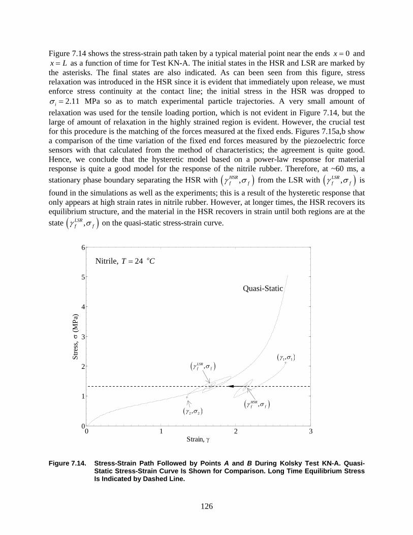
126

Figure 7.14 shows the stress-strain path taken by a typical material point near the ends 0x = and x L= as a function of time for Test KN-A. The initial states in the HSR and LSR are marked by the asterisks. The final states are also indicated. As can been seen from this figure, stress relaxation was introduced in the HSR since it is evident that immediately upon release, we must enforce stress continuity at the contact line; the initial stress in the HSR was dropped to

2.11iσ = MPa so as to match experimental particle trajectories. A very small amount of relaxation was used for the tensile loading portion, which is not evident in Figure 7.14, but the large of amount of relaxation in the highly strained region is evident. However, the crucial test for this procedure is the matching of the forces measured at the fixed ends. Figures 7.15a,b show a comparison of the time variation of the fixed end forces measured by the piezoelectric force sensors with that calculated from the method of characteristics; the agreement is quite good. Hence, we conclude that the hysteretic model based on a power-law response for material response is quite a good model for the response of the nitrile rubber. Therefore, at ~60 ms, a stationary phase boundary separating the HSR with ( ),HSR

f fγ σ from the LSR with ( ),LSRf fγ σ is

found in the simulations as well as the experiments; this is a result of the hysteretic response that only appears at high strain rates in nitrile rubber. However, at longer times, the HSR recovers its equilibrium structure, and the material in the HSR recovers in strain until both regions are at the state ( ),LSR

f fγ σ on the quasi-static stress-strain curve.

Figure 7.14. Stress-Strain Path Followed by Points A and B During Kolsky Test KN-A. Quasi-

Static Stress-Strain Curve Is Shown for Comparison. Long Time Equilibrium Stress Is Indicated by Dashed Line.

0 1 2 30

1

2

3

4

5

6

Strain, γ

Stre

ss, σ

(MPa

)

( )1 1,γ σ

( )2 2,γ σ

( ),LSRf fγ σ

( ),HSRf fγ σ

Nitrile, 24 oT C=

Quasi-Static

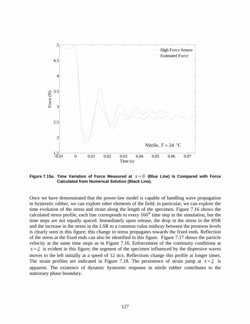
127

Figure 7.15a. Time Variation of Force Measured at 0x = (Blue Line) Is Compared with Force Calculated from Numerical Solution (Black Line).

Once we have demonstrated that the power-law model is capable of handling wave propagation in hysteretic rubber, we can explore other elements of the field; in particular, we can explore the time evolution of the stress and strain along the length of the specimen. Figure 7.16 shows the calculated stress profile; each line corresponds to every 166th time step in the simulation, but the time steps are not equally spaced. Immediately upon release, the drop in the stress in the HSR and the increase in the stress in the LSR to a common value midway between the prestress levels is clearly seen in this figure; this change in stress propagates towards the fixed ends. Reflection of the stress at the fixed ends can also be identified in this figure. Figure 7.17 shows the particle velocity at the same time steps as in Figure 7.16. Enforcement of the continuity conditions at x ξ= is evident in this figure; the segment of the specimen influenced by the dispersive waves moves to the left initially at a speed of 12 m/s. Reflections change this profile at longer times. The strain profiles are indicated in Figure 7.18. The persistence of strain jump at x ξ= is apparent. The existence of dynamic hysteretic response in nitrile rubber contributes to the stationary phase boundary.

-0.01 0 0.01 0.02 0.03 0.04 0.05 0.06 0.071.5

2

2.5

3

3.5

4

4.5

5

Time (s)

Forc

e (N

)

High Force SensorEstimated Force

Nitrile, 24 oT C=

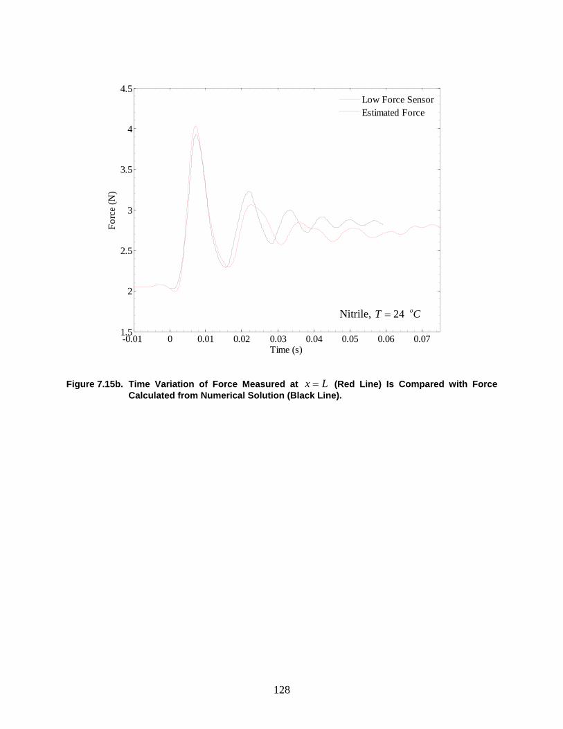
128

Figure 7.15b. Time Variation of Force Measured at x L= (Red Line) Is Compared with Force

Calculated from Numerical Solution (Black Line).

-0.01 0 0.01 0.02 0.03 0.04 0.05 0.06 0.071.5

2

2.5

3

3.5

4

4.5

Time (s)

Forc

e (N

)

Low Force SensorEstimated Force

Nitrile, 24 oT C=

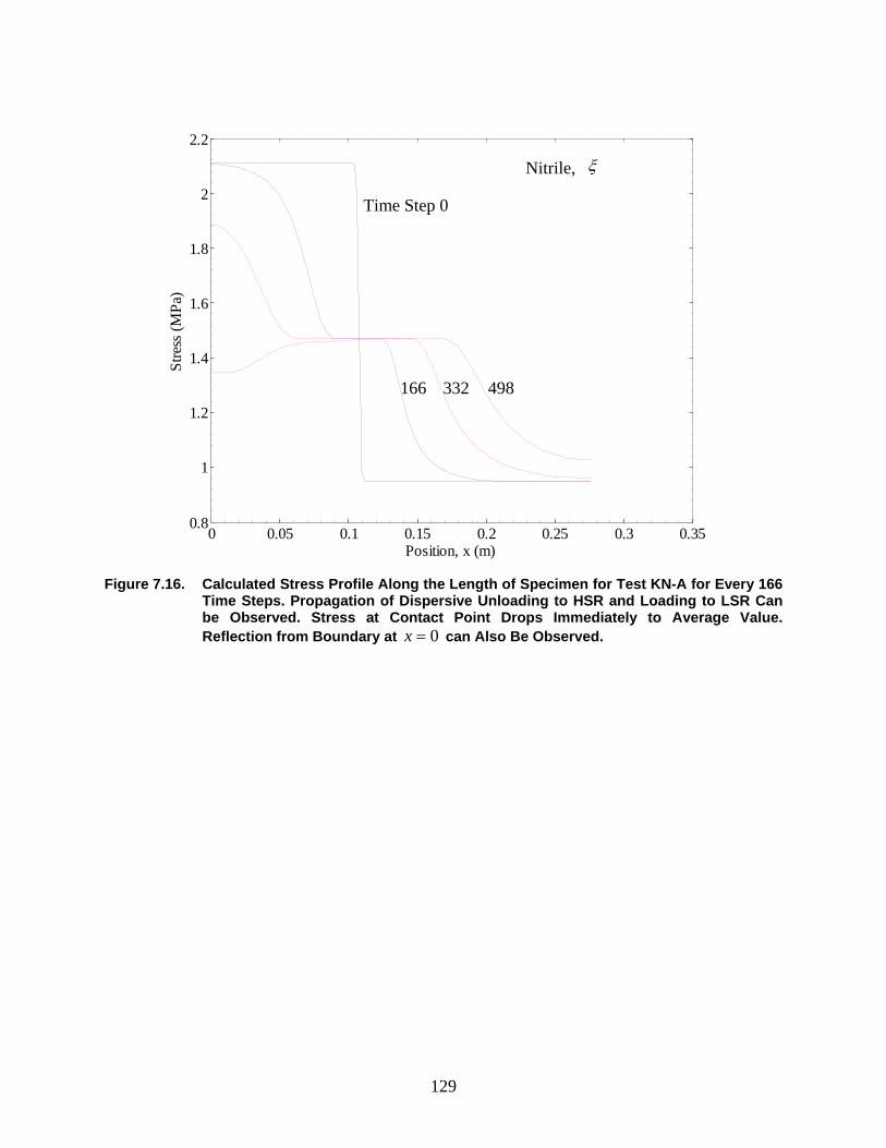
129

Figure 7.16. Calculated Stress Profile Along the Length of Specimen for Test KN-A for Every 166 Time Steps. Propagation of Dispersive Unloading to HSR and Loading to LSR Can be Observed. Stress at Contact Point Drops Immediately to Average Value. Reflection from Boundary at 0x = can Also Be Observed.

0 0.05 0.1 0.15 0.2 0.25 0.3 0.350.8

1

1.2

1.4

1.6

1.8

2

2.2

Position, x (m)

Stre

ss (M

Pa)

Nitrile, ξ

Time Step 0

166 332 498

130

Figure 7.17. Calculated Particle Velocity Along Length of Specimen for Test KN-A for Every 166 Time Steps.

0 0.05 0.1 0.15 0.2 0.25 0.3 0.35-14

-12

-10

-8

-6

-4

-2

0

Position, x (m)

Parti

cle

Vel

ocity

(m/s)

Nitrile, 24 oT C=

166 332 498

Time Step 0

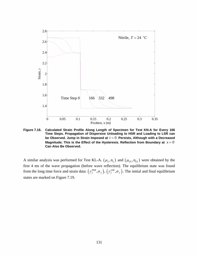
131

Figure 7.18. Calculated Strain Profile Along Length of Specimen for Test KN-A for Every 166 Time Steps. Propagation of Dispersive Unloading to HSR and Loading to LSR can be Observed. Jump in Strain Imposed at 0t = Persists, Although with a Decreased Magnitude; This Is the Effect of the Hysteresis. Reflection from Boundary at 0x = Can Also Be Observed.

A similar analysis was performed for Test KL-A. ( ),L Lnµ and ( ),UL ULnµ were obtained by the first 4 ms of the wave propagation (before wave reflection). The equilibrium state was found from the long time force and strain data: ( ),HSR

f fγ σ , ( ),LSRf fγ σ . The initial and final equilibrium

states are marked on Figure 7.19.

0 0.05 0.1 0.15 0.2 0.25 0.3 0.35

1.4

1.6

1.8

2

2.2

2.4

2.6

2.8

Position, x (m)

Stra

in, γ

Nitrile, 24 oT C=

166 332 498 Time Step 0

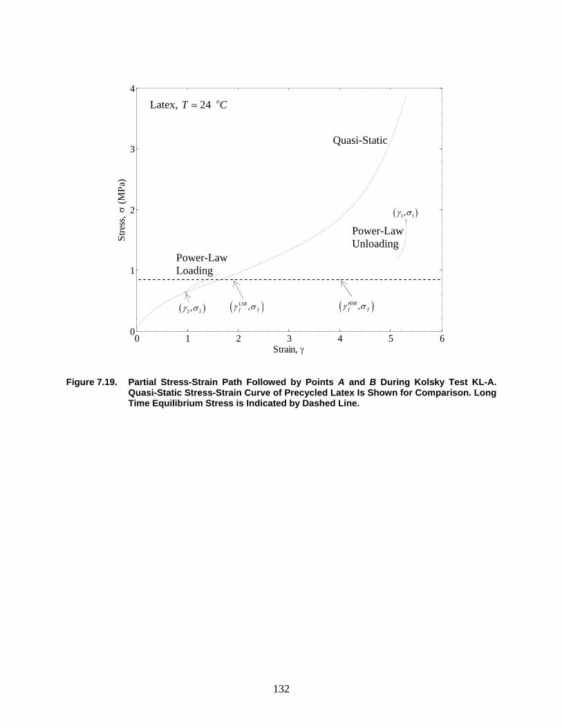
132

Figure 7.19. Partial Stress-Strain Path Followed by Points A and B During Kolsky Test KL-A.

Quasi-Static Stress-Strain Curve of Precycled Latex Is Shown for Comparison. Long Time Equilibrium Stress is Indicated by Dashed Line.

0 1 2 3 4 5 60

1

2

3

4

Strain, γ

Stre

ss, σ

(MPa

)

( )1 1,γ σ

( )2 2,γ σ

( ),LSR

f fγ σ ( ),HSRf fγ σ

Latex, 24 oT C=

Quasi-Static

Power-Law Loading

Power-Law Unloading

133

8. CONCLUSIONS In this report, we have explored the propagation of dispersive waves, shock waves, and the effect of hysteresis on the unloading response. We now present a brief summary and discussion of all the observations and models. The suggested stress-strain responses for latex and nitrile rubbers are shown in Figures 8.1 and 8.2, respectively. At strain rates above 500γ > s-1, the high strain-rate response of latex and nitrile rubbers appears to be governed by an instantaneous elastic response that can be represented by a power-law model of the form nσ µγ= . This power-law response is shown in Figures 8.1 and 8.2 by the solid lines; for comparison, the quasi-static stress-strain curve is shown by the dashed lines. µ and n depend on the material as well as the prestrain; for initially unstrained materials, the exponent was almost 0.5n = for both latex and nitrile; while we have not examined micromechanisms responsible for the power-law form, it is tempting to relate this to the relaxation behavior associated with the Rouse modes of the entanglement strands. With increasing prestrain, µ decreases while n increases, with the product remaining nearly constant; these variations suggest that the prestrain influences the mobility of the chains and therefore affects the stress-strain response. For specimens prestrained quasi-statically to levels 0 ~ 1.5γ > , three types of responses are observed. If the impact speed is less than the critical velocity

I

CJVγ , once again, dispersive waves that can be represented by the

power-law model are generated; in cases when I

CJV Vγ≥ , shock waves are formed, and the material response jumps from an initial state that lies on the quasi-static stress-strain curve to the tangent point on the tensile shock adiabat. Further straining occurs following a new power-law model that corresponds to the “transformed” material. The tensile shock adiabat for latex and nitrile rubbers is shown in Figures 8.1 and 8.2, respectively by the thick dash-dot lines; it is clear that the shock end states are at significantly higher stress levels than the quasi-static or even the dynamic shock-free response. In particular, it is important to recognize that under continued high strain rate loading, the dynamic stress-strain response deviates significantly from the quasi-static counterpart, and in some cases, the dynamic stress is lower than the quasi-static values. This suggests that mechanisms of damage may have been triggered under dynamic loading that was not activated in the slower rate loading. These issues require further study, with diagnostic tools that reveal structural changes as well as the macroscopic strains. The unloading response exhibited interesting hysteresis, but with the analysis based on dispersive and shock waves developed above, it is possible to model the unloading response. The most remarkable feature of the hysteresis is that the energy “stored” in the rubber during quasi-static loading is not recovered when subjected to a rapid release. While strain-induced crystallization may be considered to play a role in the latex rubber, the existence of such dynamic hysteresis in nonstrain-crystallizing nitrile rubber suggests that crystallization may only be a part of the influence. Structural rearrangement within the amorphous phase and the inability to rapidly recover the equilibrium chain packing structure may also contribute significantly to the hysteretic response.

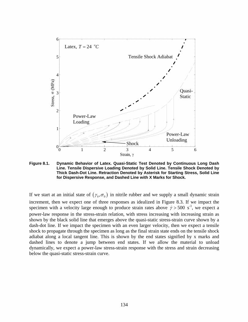
134

Figure 8.1. Dynamic Behavior of Latex. Quasi-Static Test Denoted by Continuous Long Dash

Line. Tensile Dispersive Loading Denoted by Solid Line. Tensile Shock Denoted by Thick Dash-Dot Line. Retraction Denoted by Asterisk for Starting Stress, Solid Line for Dispersive Response, and Dashed Line with X Marks for Shock.

If we start at an initial state of ( )0 0,γ σ in nitrile rubber and we supply a small dynamic strain increment, then we expect one of three responses as idealized in Figure 8.3. If we impact the specimen with a velocity large enough to produce strain rates above 500γ > s-1, we expect a power-law response in the stress-strain relation, with stress increasing with increasing strain as shown by the black solid line that emerges above the quasi-static stress-strain curve shown by a dash-dot line. If we impact the specimen with an even larger velocity, then we expect a tensile shock to propagate through the specimen as long as the final strain state ends on the tensile shock adiabat along a local tangent line. This is shown by the end states signified by x marks and dashed lines to denote a jump between end states. If we allow the material to unload dynamically, we expect a power-law stress-strain response with the stress and strain decreasing below the quasi-static stress-strain curve.

0 1 2 3 4 5 60

1

2

3

4

5

6

Strain, γ

Stre

ss, σ

(MPa

)

Quasi-Static

Latex, 24 oT C=

Power-Law Loading

Tensile Shock Adiabat

Power-Law Unloading

Shock

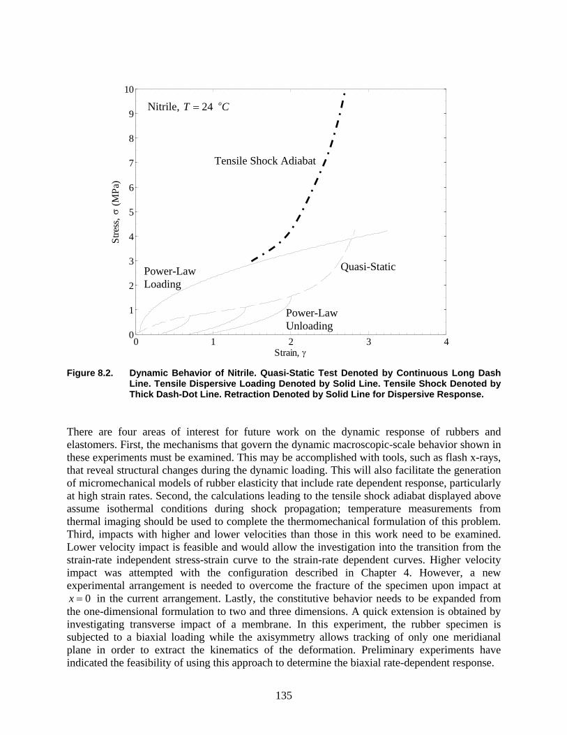
135

Figure 8.2. Dynamic Behavior of Nitrile. Quasi-Static Test Denoted by Continuous Long Dash Line. Tensile Dispersive Loading Denoted by Solid Line. Tensile Shock Denoted by Thick Dash-Dot Line. Retraction Denoted by Solid Line for Dispersive Response.

There are four areas of interest for future work on the dynamic response of rubbers and elastomers. First, the mechanisms that govern the dynamic macroscopic-scale behavior shown in these experiments must be examined. This may be accomplished with tools, such as flash x-rays, that reveal structural changes during the dynamic loading. This will also facilitate the generation of micromechanical models of rubber elasticity that include rate dependent response, particularly at high strain rates. Second, the calculations leading to the tensile shock adiabat displayed above assume isothermal conditions during shock propagation; temperature measurements from thermal imaging should be used to complete the thermomechanical formulation of this problem. Third, impacts with higher and lower velocities than those in this work need to be examined. Lower velocity impact is feasible and would allow the investigation into the transition from the strain-rate independent stress-strain curve to the strain-rate dependent curves. Higher velocity impact was attempted with the configuration described in Chapter 4. However, a new experimental arrangement is needed to overcome the fracture of the specimen upon impact at

0x = in the current arrangement. Lastly, the constitutive behavior needs to be expanded from the one-dimensional formulation to two and three dimensions. A quick extension is obtained by investigating transverse impact of a membrane. In this experiment, the rubber specimen is subjected to a biaxial loading while the axisymmetry allows tracking of only one meridianal plane in order to extract the kinematics of the deformation. Preliminary experiments have indicated the feasibility of using this approach to determine the biaxial rate-dependent response.

0 1 2 3 40

1

2

3

4

5

6

7

8

9

10

Strain, γ

Stre

ss, σ

(MPa

)Nitrile, 24 oT C=

Power-Law Loading

Tensile Shock Adiabat

Quasi-Static

Power-Law Unloading

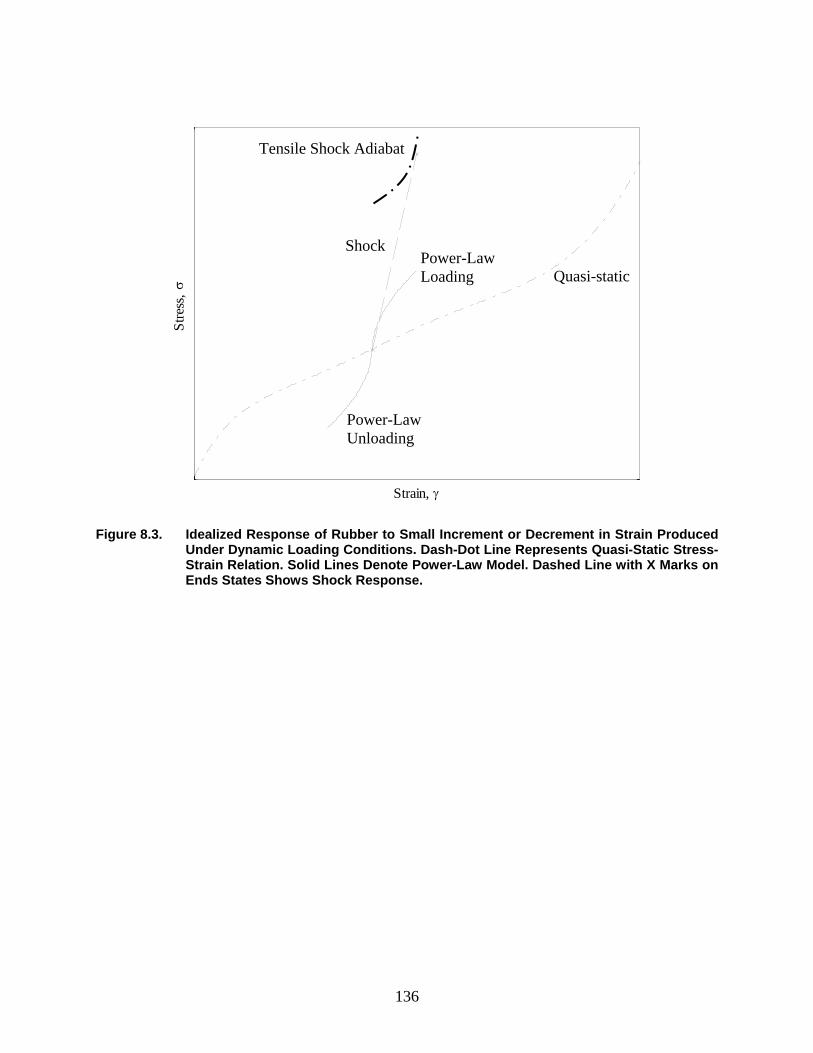
136

Figure 8.3. Idealized Response of Rubber to Small Increment or Decrement in Strain Produced Under Dynamic Loading Conditions. Dash-Dot Line Represents Quasi-Static Stress-Strain Relation. Solid Lines Denote Power-Law Model. Dashed Line with X Marks on Ends States Shows Shock Response.

Strain, γ

Stre

ss, σ

Power-Law Unloading

Power-Law Loading

Shock

Tensile Shock Adiabat

Quasi-static

137

9. REFERENCES Abeyaratne, R., and J.K. Knowles, Evolution of Phase Transitions; A Continuum Theory, Cambridge University Press, Cambridge, 2006. Bogoslovov, R.B., and C.M. Roland, Viscoelastic effects on the free retraction of rubber, Journal of Applied Physics, 102, 063531, 2007. Cristescu, N., Dynamic Plasticity, North-Holland Publishing Company, Amsterdam, 56-66, 1967. Graff, K.F., Wave Motion in Elastic Solids, Dover Publications, New York, 1975. Hoo Fatt, M.S., and I. Bekar, High-speed testing and material modeling of unfilled styrene butadiene vulcanizates at impact rates, Journal of Materials Science, 39, 6885-6899, 2004. Hoo Fatt, M.S., and X. Ouyang, Three-dimensional constitutive equations for Styrene Butadiene Rubber at high strain rates, Mechanics of Materials, 40, 1-16, 2008. Igra, O., L. Wang, G. Ben-Dor, H. Reichenback, and W. Hellig, Uni-axial strain loading of a rubber rod by planar shock waves, Acta Mechanica, 120, 91-107, 1997. Ivanov, A.G., and S.A. Novikov, Rarefaction shock waves in iron and steel, Soviet Physics JETP, 13, 1321-1323, 1961. Knowles, J.K., Impact-induced tensile waves in a rubberlike material. SIAM Journal of Applied Mathematics, 62, 1153-1175, 2002. Knowles, J.K., Sudden tensile loading of a rubberlike bar. Mechanics Research Communications, 30, 581-587, 2003. Kolsky, H., Production of tensile shock waves in stretched natural rubber. Nature. 224, 1301, 1969. Kolsky, H., and L.S. Douch, Experimental studies in plastic wave propagation, Journal of the Mechanics and Physics of Solids, 10, 195-223, 1962. Landau, L.D., and E.M. Lifshitz, Fluid Mechanics, Elsevier, Amsterdam, 489-494, 2004. Mason, P., Finite elastic wave propagation in rubber. Proceedings of the Royal Society of London. Series A, Mathematical and Physical Sciences, 272, 315-330, 1963. Miyamoto, Y., H. Yamao, and K. Sekimoto, Crystallization and melting of polyisoprene rubber under uniaxial deformation, Macromolecules, 36, 6462-6471, 2003. Mott, P.H., J.N. Twigg, D.F. Roland, H.S. Schrader, J.A. Pathak, and C.M. Roland, High-speed tensile test, Review of Scientific Instruments, 78, 045105, 2007.

138

Mrowca, B.A., S. Dart and E. Guth, Photographic study of the retraction of stressed rubber, Physical Review, 66, 32, 1944. Rakhmatulin, K.A., Propagation of an unloading wave (in Russian), Prikladnaia Matematika i Mekhanika, 9, 91-100, 1945. Roland, C.M., Mechanical behavior of rubber at high strain rates, Rubber Chemistry and Technology, 79, 429-459, 2006. Rubenstein, M., and R.H. Colby, Polymer Physics, Oxford University Press, Oxford, UK, 2003. Song, B., and W. Chen, One-dimensional dynamic compressive behavior of EPDM rubber, Journal of Engineering Materials and Technology, 125, 294-301, 2003. Sutherland, H.J., Stress wave propagation in an RTV rubber. Transaction of the Society of Rheology, 20, 409-422, 1976. Taylor, G.I., The plastic wave in a wire extended by an impact load, The Scientific Papers of G. I. Taylor, Vol. I., Mechanics of Solids, University Press, 467-479, 1958. Toki, S., I. Sics, S. Ran, L. Liu, B.S. Hsiao, S. Murakami, K. Senoo and S. Kohjiya, New insights into structural development in natural rubber during uniaxial deformation by in-situ synchrotron x-ray diffraction, Macromolecules, 35, 6578-6584, 2002. Treloar, L.R.G., Physics of Rubber Elasticity (Monographs on the Physics & Chemistry of Materials), Oxford University Press; Oxford, UK, 1975. von Karman, T., and P. Duwez, The propagation of plastic deformation in solids, Journal of Applied Physics, 21, 987-994, 1950. Wall, F.T., Statistical lengths of rubber-like hydrocarbon molecules. Journal of Chemical Physics, 11, 67-71, 1943. Zel’dovich, Ya. B., and Yu. P. Raizer, Physics of Shock-Waves and High-Temperature Hydrodynamic Phenomena, (Edited by W.D. Hayes and R.F. Probstein), Dover Publications, p. 757-762, 2002. Zhang, H.P., J. Niemczura, G. Dennis, K. Ravi-Chandar, and M. Marder, Toughening effect of strain-induced crystallites in natural rubber, Physical Review Letters, 142, Article ID 245503, 2009. J.A. Zukas, (Editor), High Velocity Impact Dynamics, John Wiley and Sons, Inc., New York, 1990.

139

APPENDIX A: RIEMANN NUMERICAL SIMULATION We conducted a study on the use of the Riemann solution using Riemann invariants in terms of strain are carried out on the tensile impact of latex rubber. This test has slightly different parameters than were shown in Figure 4.2. The horizontal resolution is 7,742 pixels per meter, and the vertical resolution is 250,000 pixels per second. The latex rubber had an initial strain of

0.06γ = , and the closed form solution was fitted using 0.97µ = MPa and 0.54n = . In regards to implementing the Riemann solution, an additional piece of information is needed: the impact velocity. Measuring the particle displacements in the y t− diagram where the particles are determined to be moving at a constant velocity, the impact velocity is 42 m/s. Figure A.1 shows the Riemann solution plotted in red lines on top of the y t− diagram. There several factors that can be varied and used in this calculation. The first and foremost is node locations. Each red line corresponds to a node location corresponding to the physical locations of the markers. What is not shown are the additional nodes in between the nodes displaced by the red lines. In between each red line, there are nine additional nodes. The same approximate spacing of nodes is continued from the right red line shown to the fixed end far to the right of this image with the total length of the specimen being 0.3 meter long. As a note, this node spacing is not uniform across the entire specimen due to the fact that the black lines in the experiment are not exactly 5 mm apart from one another. 1.6β = is used to satisfy the Courant condition. The location of x− and x+ are determined by

.j

j

x x c dt

x x c dt− −

+ +

= +

= − (A-1)

At this point, we examine the calculation of the characteristics, kc− and kc+ . One method is to approximate the locations x− and x+ using the wave speed at node j and then interpolate kc− and

kc+ based on these calculated locations x− and x+ using the jc at all the nodes along the length of the specimen. A second method begins with an interpolation of kc− and kc+ and not an approximation of x− and x+ . First we examine the calculation of kc+ . We define α + as

1

1

i i i

i i i

c c c cx x x x

α + −+

+ −

− −≡ =

− −. (A-2)

We also know that the relation between x+ and ix ,

ic dt x x+ += − . (A-3)

140

Plugging Eq (A-3) into Eq. (A-2), we get

ic cc dt

α ++

+

−= . (A-4)

Rearranging Eq. (A-4), we arrive at the explicit expression for c+ ,

( )1icc

dtα++

=+

. (A-5)

Following the same procedure, we can find the expression for c− ,

( )

1

1

.1

i i

i i

i

c cx x

ccdt

+−

−

−−

−≡

−

=+

α

α

(A-6)

Figure A.1. Riemann Solution for Tensile Impact of Specimen DL-C.

0 50 100 150 200 250 300 350 400 4500

100

200

300

400

500

600

700

Position, y (pixels)

Tim

e, t

(pix

els)

(58 mm)

(2.8 ms) Latex, 24 oT C=

141

In Figure A.1, c− and c+ are calculated using Eqs. (A-4) and (A-6). The importance of node spacing, the value of β , and how c− and c+ are calculated, as well as the initial wave speed specified, will be investigated shortly. We see that this Riemann solution matches the experimental results fairly well. With the last red line on the right, we see an increased separation between the particle displacement prediction from the solution and the actual displacement for a small section of time. If we associate this section with respect to a certain range of wave speeds, we see that previous red lines also show this separation, although not to the extent seen with the last line. Another deviation seen is when the particles are displacing with a constant velocity. Once again, as the red lines increase in distance from impact location, we see a more marked departure from the experimental results, with calculated trajectories displacing a little further than experiment results in this constant sector. Now we compare the Riemann solution to the closed form solution. Figure A.2 shows the Riemann solution with a solid, black line and the closed form solution with a dashed, red line. The y t− diagram is not shown. While the Riemann solution and closed form solution match each other fairly closely as well as the experiment, it can be seen that in the Riemann solution, the particles displace a little more than predicted in the closed form solution for a segment of

Figure A.2. Comparison of Riemann Solution (Solid Black Lines) to Closed Form Solution (Dashed Red Lines) for Tensile Impact of Specimen DL-C.

0 0.01 0.02 0.03 0.04 0.05 0.060

1

2

3

Position, y (m)

Tim

e, t

(ms)

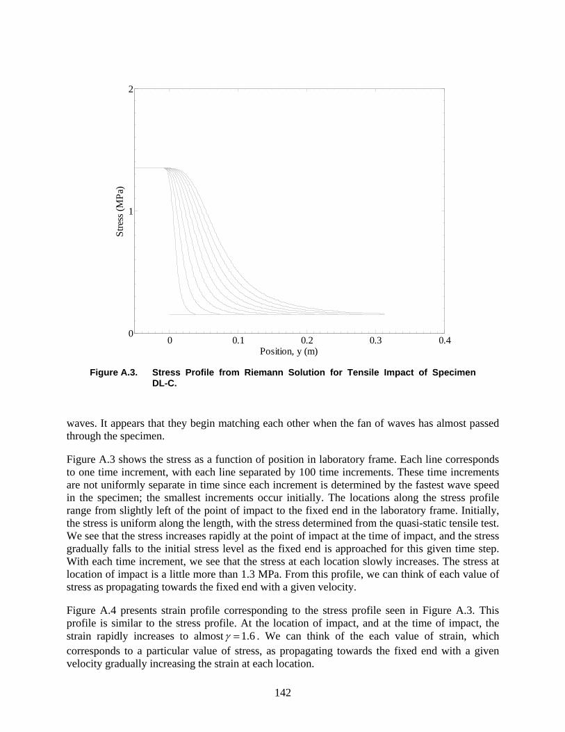
142

waves. It appears that they begin matching each other when the fan of waves has almost passed through the specimen. Figure A.3 shows the stress as a function of position in laboratory frame. Each line corresponds to one time increment, with each line separated by 100 time increments. These time increments are not uniformly separate in time since each increment is determined by the fastest wave speed in the specimen; the smallest increments occur initially. The locations along the stress profile range from slightly left of the point of impact to the fixed end in the laboratory frame. Initially, the stress is uniform along the length, with the stress determined from the quasi-static tensile test. We see that the stress increases rapidly at the point of impact at the time of impact, and the stress gradually falls to the initial stress level as the fixed end is approached for this given time step. With each time increment, we see that the stress at each location slowly increases. The stress at location of impact is a little more than 1.3 MPa. From this profile, we can think of each value of stress as propagating towards the fixed end with a given velocity. Figure A.4 presents strain profile corresponding to the stress profile seen in Figure A.3. This profile is similar to the stress profile. At the location of impact, and at the time of impact, the strain rapidly increases to almost 1.6γ = . We can think of the each value of strain, which corresponds to a particular value of stress, as propagating towards the fixed end with a given velocity gradually increasing the strain at each location.

Figure A.3. Stress Profile from Riemann Solution for Tensile Impact of Specimen DL-C.

0 0.1 0.2 0.3 0.40

1

2

Position, y (m)

Stre

ss (M

Pa)

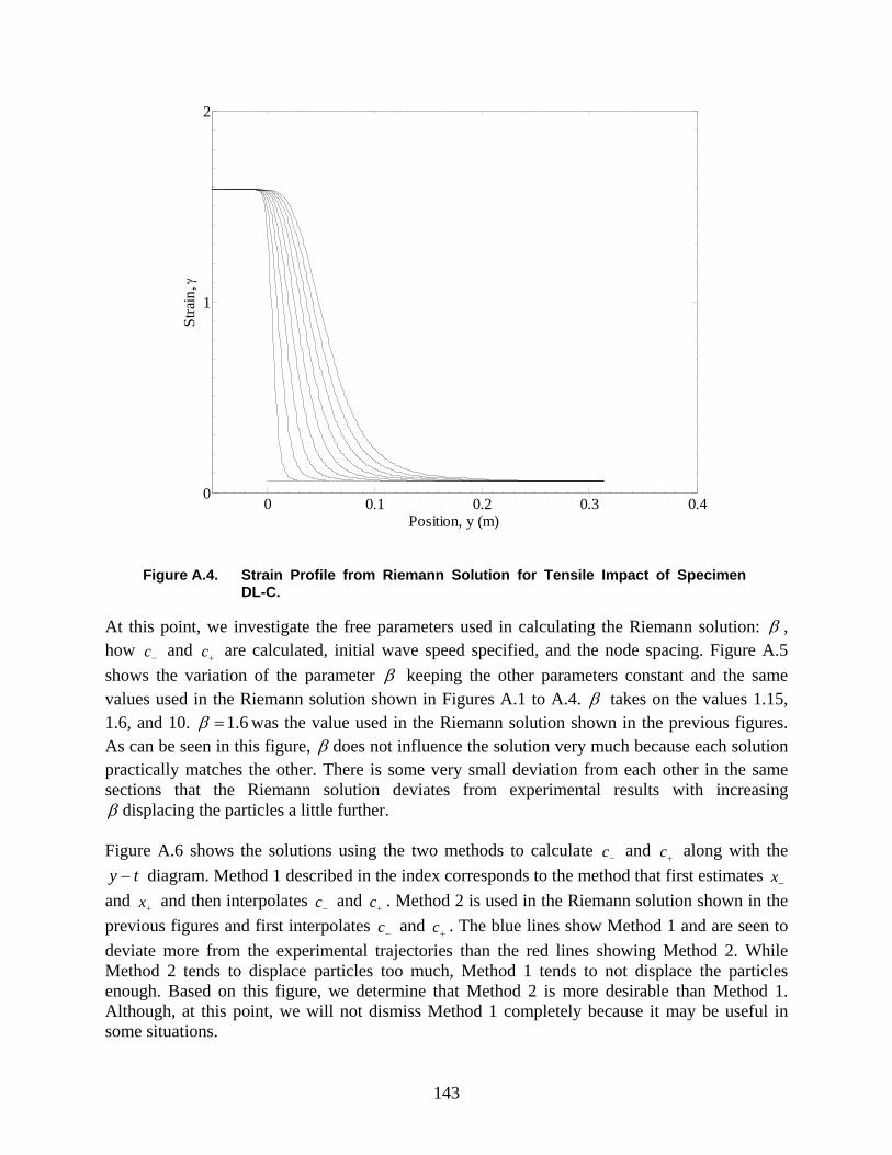
143

At this point, we investigate the free parameters used in calculating the Riemann solution: β , how c− and c+ are calculated, initial wave speed specified, and the node spacing. Figure A.5 shows the variation of the parameter β keeping the other parameters constant and the same values used in the Riemann solution shown in Figures A.1 to A.4. β takes on the values 1.15, 1.6, and 10. 1.6β = was the value used in the Riemann solution shown in the previous figures. As can be seen in this figure, β does not influence the solution very much because each solution practically matches the other. There is some very small deviation from each other in the same sections that the Riemann solution deviates from experimental results with increasing β displacing the particles a little further. Figure A.6 shows the solutions using the two methods to calculate c− and c+ along with the y t− diagram. Method 1 described in the index corresponds to the method that first estimates x− and x+ and then interpolates c− and c+ . Method 2 is used in the Riemann solution shown in the previous figures and first interpolates c− and c+ . The blue lines show Method 1 and are seen to deviate more from the experimental trajectories than the red lines showing Method 2. While Method 2 tends to displace particles too much, Method 1 tends to not displace the particles enough. Based on this figure, we determine that Method 2 is more desirable than Method 1. Although, at this point, we will not dismiss Method 1 completely because it may be useful in some situations.

Figure A.4. Strain Profile from Riemann Solution for Tensile Impact of Specimen DL-C.

0 0.1 0.2 0.3 0.40

1

2

Position, y (m)

Stra

in, γ

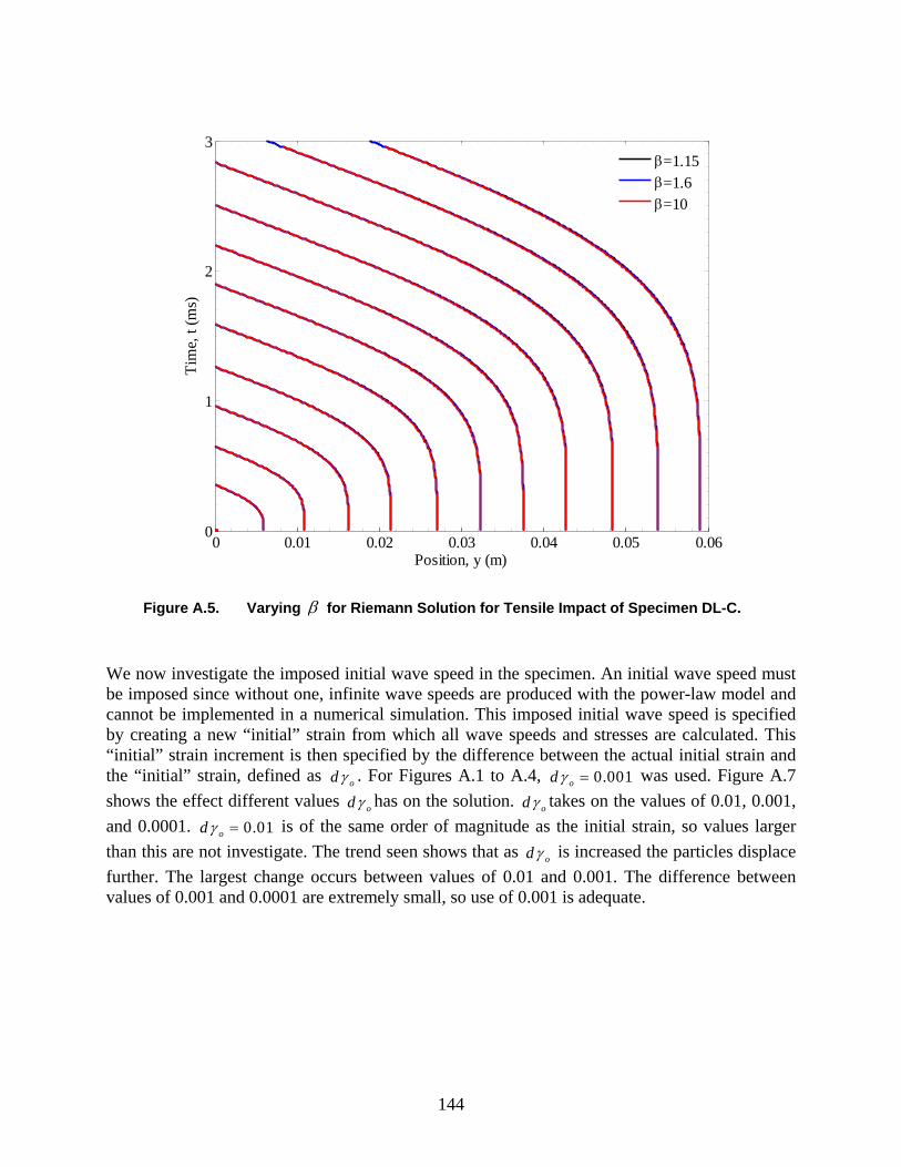
144

We now investigate the imposed initial wave speed in the specimen. An initial wave speed must be imposed since without one, infinite wave speeds are produced with the power-law model and cannot be implemented in a numerical simulation. This imposed initial wave speed is specified by creating a new “initial” strain from which all wave speeds and stresses are calculated. This “initial” strain increment is then specified by the difference between the actual initial strain and the “initial” strain, defined as odγ . For Figures A.1 to A.4, 0.001odγ = was used. Figure A.7 shows the effect different values odγ has on the solution. odγ takes on the values of 0.01, 0.001, and 0.0001. 0.01odγ = is of the same order of magnitude as the initial strain, so values larger than this are not investigate. The trend seen shows that as odγ is increased the particles displace further. The largest change occurs between values of 0.01 and 0.001. The difference between values of 0.001 and 0.0001 are extremely small, so use of 0.001 is adequate.

Figure A.5. Varying β for Riemann Solution for Tensile Impact of Specimen DL-C.

0 0.01 0.02 0.03 0.04 0.05 0.060

1

2

3

Position, y (m)

Tim

e, t

(ms)

β=1.15β=1.6β=10

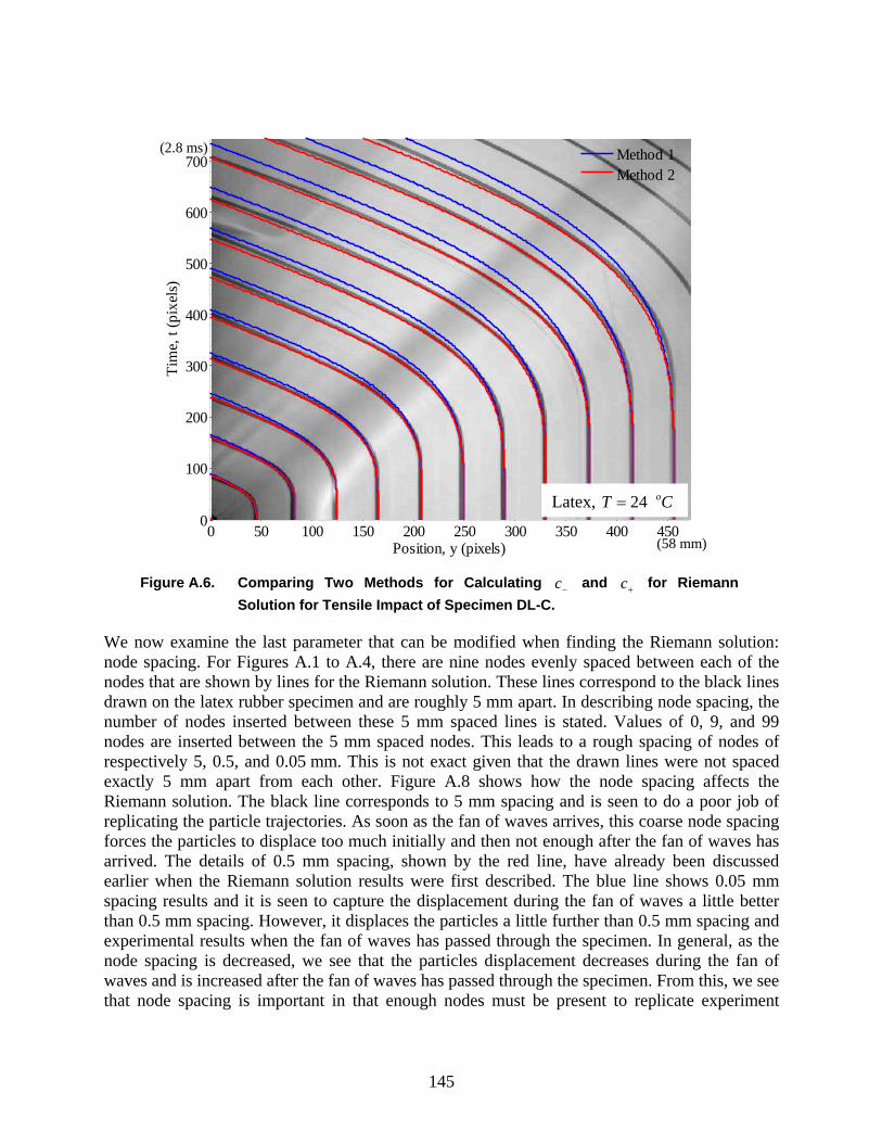
145

We now examine the last parameter that can be modified when finding the Riemann solution: node spacing. For Figures A.1 to A.4, there are nine nodes evenly spaced between each of the nodes that are shown by lines for the Riemann solution. These lines correspond to the black lines drawn on the latex rubber specimen and are roughly 5 mm apart. In describing node spacing, the number of nodes inserted between these 5 mm spaced lines is stated. Values of 0, 9, and 99 nodes are inserted between the 5 mm spaced nodes. This leads to a rough spacing of nodes of respectively 5, 0.5, and 0.05 mm. This is not exact given that the drawn lines were not spaced exactly 5 mm apart from each other. Figure A.8 shows how the node spacing affects the Riemann solution. The black line corresponds to 5 mm spacing and is seen to do a poor job of replicating the particle trajectories. As soon as the fan of waves arrives, this coarse node spacing forces the particles to displace too much initially and then not enough after the fan of waves has arrived. The details of 0.5 mm spacing, shown by the red line, have already been discussed earlier when the Riemann solution results were first described. The blue line shows 0.05 mm spacing results and it is seen to capture the displacement during the fan of waves a little better than 0.5 mm spacing. However, it displaces the particles a little further than 0.5 mm spacing and experimental results when the fan of waves has passed through the specimen. In general, as the node spacing is decreased, we see that the particles displacement decreases during the fan of waves and is increased after the fan of waves has passed through the specimen. From this, we see that node spacing is important in that enough nodes must be present to replicate experiment

Figure A.6. Comparing Two Methods for Calculating c− and c+ for Riemann Solution for Tensile Impact of Specimen DL-C.

0 50 100 150 200 250 300 350 400 4500

100

200

300

400

500

600

700

Position, y (pixels)

Tim

e, t

(pix

els)

Method 1Method 2

(58 mm)

(2.8 ms)

Latex, 24 oT C=

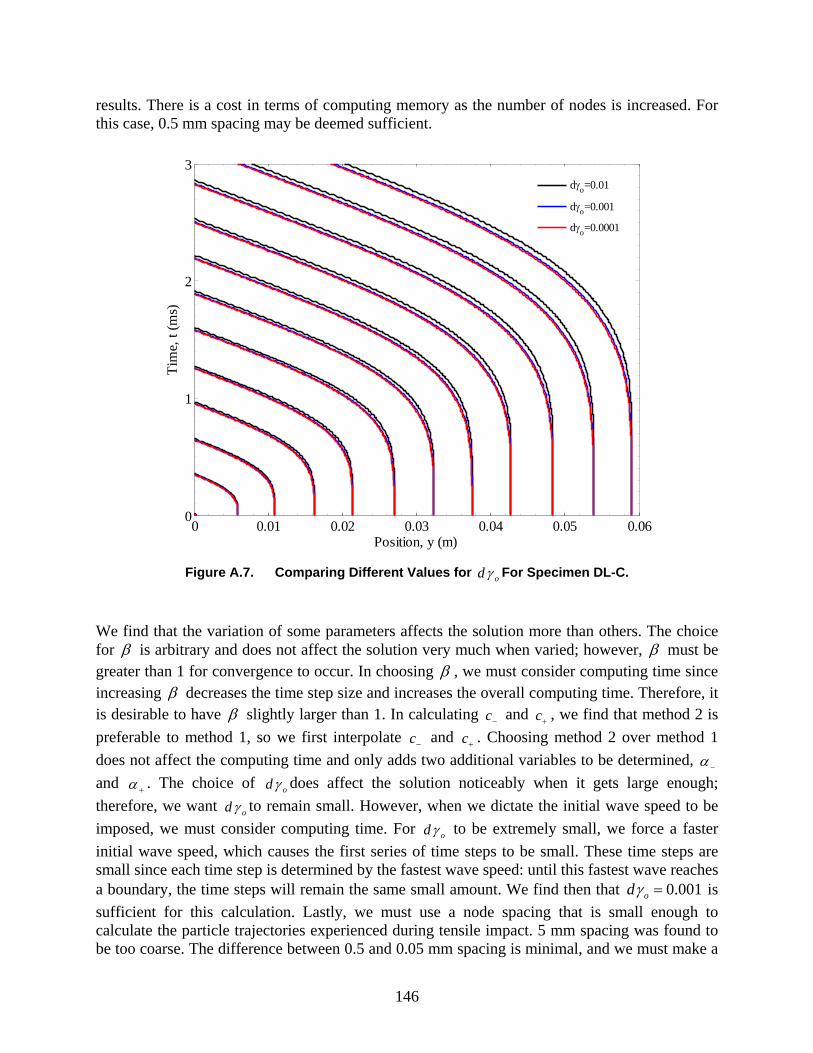
146

results. There is a cost in terms of computing memory as the number of nodes is increased. For this case, 0.5 mm spacing may be deemed sufficient.

Figure A.7. Comparing Different Values for odγ For Specimen DL-C.

We find that the variation of some parameters affects the solution more than others. The choice for β is arbitrary and does not affect the solution very much when varied; however, β must be greater than 1 for convergence to occur. In choosing β , we must consider computing time since increasing β decreases the time step size and increases the overall computing time. Therefore, it is desirable to have β slightly larger than 1. In calculating c− and c+ , we find that method 2 is preferable to method 1, so we first interpolate c− and c+ . Choosing method 2 over method 1 does not affect the computing time and only adds two additional variables to be determined, α − and α + . The choice of odγ does affect the solution noticeably when it gets large enough; therefore, we want odγ to remain small. However, when we dictate the initial wave speed to be imposed, we must consider computing time. For odγ to be extremely small, we force a faster initial wave speed, which causes the first series of time steps to be small. These time steps are small since each time step is determined by the fastest wave speed: until this fastest wave reaches a boundary, the time steps will remain the same small amount. We find then that 0.001odγ = is sufficient for this calculation. Lastly, we must use a node spacing that is small enough to calculate the particle trajectories experienced during tensile impact. 5 mm spacing was found to be too coarse. The difference between 0.5 and 0.05 mm spacing is minimal, and we must make a

0 0.01 0.02 0.03 0.04 0.05 0.060

1

2

3

Position, y (m)

Tim

e, t

(ms)

dγo=0.01

dγo=0.001

dγo=0.0001

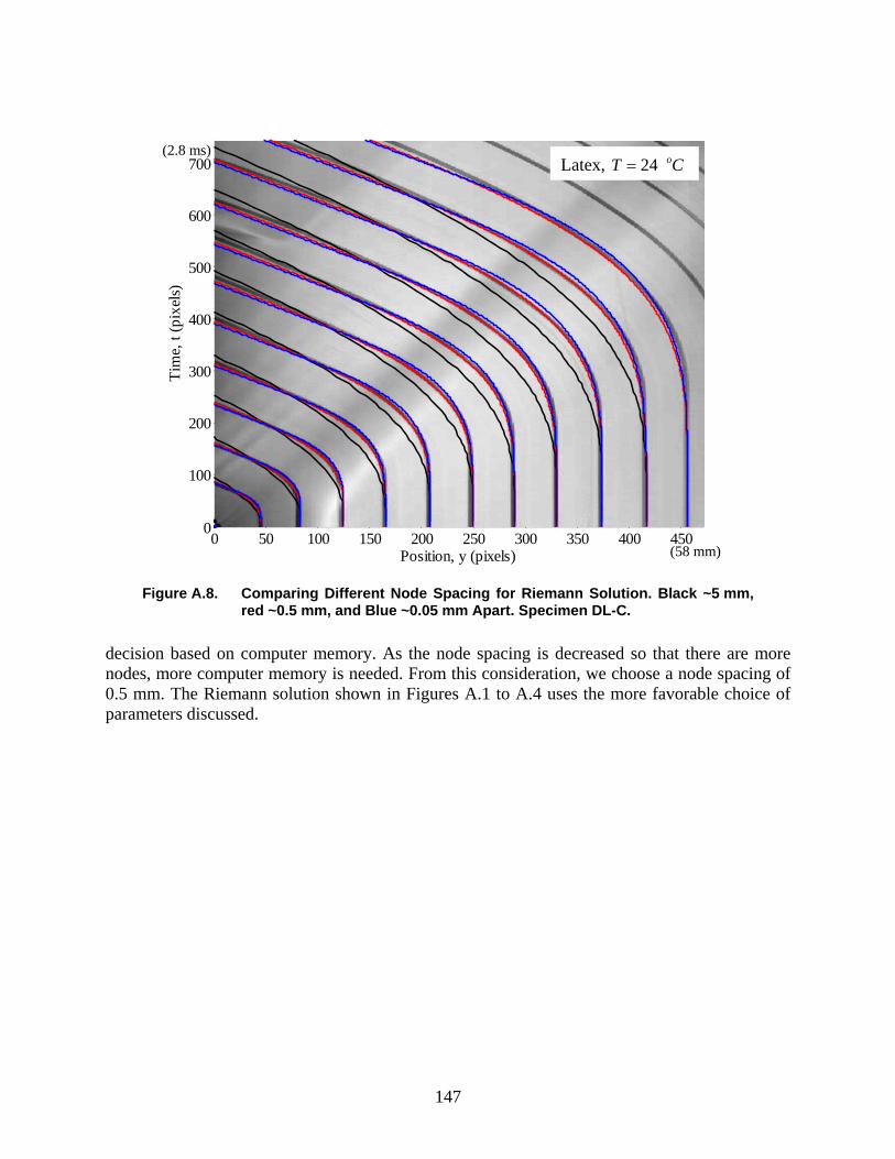
147

decision based on computer memory. As the node spacing is decreased so that there are more nodes, more computer memory is needed. From this consideration, we choose a node spacing of 0.5 mm. The Riemann solution shown in Figures A.1 to A.4 uses the more favorable choice of parameters discussed.

Figure A.8. Comparing Different Node Spacing for Riemann Solution. Black ~5 mm, red ~0.5 mm, and Blue ~0.05 mm Apart. Specimen DL-C.

0 50 100 150 200 250 300 350 400 4500

100

200

300

400

500

600

700

Position, y (pixels)

Tim

e, t

(pix

els)

(58 mm)

(2.8 ms) Latex, 24 oT C=

148

DISTRIBUTION Distributed electronically External: Lawrence Livermore National Laboratory Attn: N. Dunipace P.O. Box 808, MS L-795 Livermore, CA 94551-0808 J. G. Niemczura University of Texas-Austin Campus Executive Fellow Internal: sanddocs@sandia.gov 1 MS0123 D. Chavez, LDRD Office, 1011 1 MS0372 J. M. Redmond, 1525 1 MS0372 H. E. Fang, 1524 1 MS0372 W. M. Scherzinger, 1524 1 MS0372 J. T. Ostien, 1524 1 MS0384 A. C. Ratzel, 1500 1 MS0431 J. Pott, 0511 1 MS0899 Technical Library, 9536 (electronic copy)