On the relation between matrix-geometric and discrete ... · A discrete phase-type distribution...
60
On the relation between matrix-geometric and discrete phase-type distributions Sietske Greeuw Kongens Lyngby/Amsterdam 2009 Master thesis Mathematics University of Amsterdam
Transcript of On the relation between matrix-geometric and discrete ... · A discrete phase-type distribution...
On the relation betweenmatrix-geometric
anddiscrete phase-type
distributions
Sietske Greeuw
Kongens Lyngby/Amsterdam 2009Master thesis MathematicsUniversity of Amsterdam

Technical University of DenmarkInformatics and Mathematical ModellingBuilding 321, DK-2800 Kongens Lyngby, DenmarkPhone +45 45253351, Fax +45 [email protected]
University of AmsterdamFaculty of ScienceScience Park 404, 1098 XH Amsterdam, The NetherlandsPhone +32 20 5257678, Fax +31 20 [email protected]
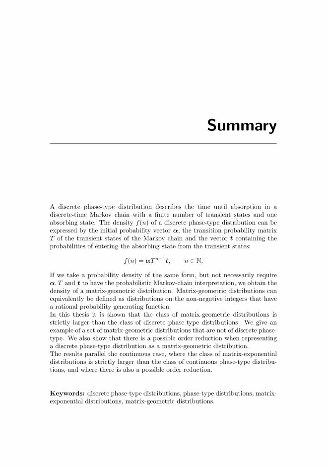
Summary
A discrete phase-type distribution describes the time until absorption in adiscrete-time Markov chain with a finite number of transient states and oneabsorbing state. The density f(n) of a discrete phase-type distribution can beexpressed by the initial probability vector α, the transition probability matrixT of the transient states of the Markov chain and the vector t containing theprobabilities of entering the absorbing state from the transient states:
f(n) = αTn−1t, n ∈ N.
If we take a probability density of the same form, but not necessarily requireα, T and t to have the probabilistic Markov-chain interpretation, we obtain thedensity of a matrix-geometric distribution. Matrix-geometric distributions canequivalently be defined as distributions on the non-negative integers that havea rational probability generating function.In this thesis it is shown that the class of matrix-geometric distributions isstrictly larger than the class of discrete phase-type distributions. We give anexample of a set of matrix-geometric distributions that are not of discrete phase-type. We also show that there is a possible order reduction when representinga discrete phase-type distribution as a matrix-geometric distribution.The results parallel the continuous case, where the class of matrix-exponentialdistributions is strictly larger than the class of continuous phase-type distribu-tions, and where there is also a possible order reduction.
Keywords: discrete phase-type distributions, phase-type distributions, matrix-exponential distributions, matrix-geometric distributions.
ii
Resume
En diskret fasetype fordeling er fordelingen af tiden til absorption i en diskret-tids Markov kæde med et begrænset antal transiente tilstande og en absorbe-rende tilstand. Tætheden f(n) af en diskret fasetype fordeling kan udtrykkes vedvektoren med den initielle fordeling α, matricen T, der beskriver de mulige over-gange mellem transiente tilstande i Markov kæden, og vektoren t med sandsyn-ligheder for at springe til den absorberende tilstand fra de transiente tilstande:
f(n) = αTn−1t, n ∈ N.
Hvis vi tager en tæthed af samme form, men ikke nødvendigvis kræver, atα, T og t har probabilistisk Markov kæde fortolkning, far vi tætheden af enmatrix-geometrisk fordeling. Matrix-geometriske fordelinger kan tilsvarende de-fineres som fordelinger pa ikke-negative heltal, der har en rationel sandsyn-lighedsgenererende funktion.I denne projekt er det vist, at mængden af matrix-geometriske fordelinger erstrengt større end mængden af diskrete fasetype fordelinger. Der gives et ek-sempel pa en mængde af matrix-geometriske fordelinger, der ikke er af diskretfasetype. Vi viser ogsa, at der er en mulighed for reduktion af størrelse afrepræsentationen, nar de repræsenterer en diskret fasetype fordeling som enmatrix-geometrisk fordeling.Resultaterne svarer til det kontinuerte tilfælde, hvor klassen af matrix-eksponentielle fordelinger er strengt større end klassen af kontinuert fasetypefordelinger, og hvor reduktion af størrelse af repræsentation ogsa er muligt.

iv

Preface
This thesis was prepared in partial fulfillment of the requirements for acquiringthe master of science degree in Mathematics. It has been prepared during afive month Erasmus-stay at the Danish Technical University, at the institute forInformatics and Mathematical Modelling.
I would like to thank my two supervisors, Bo Friis Nielsen and Michel Mandjes,for both being very supportive in my decision of doing my master project abroad.Furthermore I want to thank Bo for his friendly and informative guidance, andMichel for his help with the final parts of my thesis.
Finally I want to thank my family and my friends and all other people who havesupported me during this process.
Amsterdam, March 2009
Sietske Greeuw
vi
Contents
Summary i
Resume iii
Preface v
1 Introduction 1
2 Phase-type distributions 52.1 Discrete phase-type distributions . . . . . . . . . . . . . . . . . . 52.2 Continuous phase-type distributions . . . . . . . . . . . . . . . . 19
3 Matrix-exponential distributions 233.1 Definition . . . . . . . . . . . . . . . . . . . . . . . . . . . . . . . 243.2 Examples of matrix-exponential distributions . . . . . . . . . . . 25
4 Matrix-geometric distributions 314.1 Definition . . . . . . . . . . . . . . . . . . . . . . . . . . . . . . . 324.2 Existence of genuine matrix-geometric distributions . . . . . . . . 344.3 Order reduction for matrix-geometric distributions . . . . . . . . 384.4 Properties of matrix-geometric distributions . . . . . . . . . . . . 45

viii CONTENTS

Chapter 1
Introduction
In this thesis the relation between matrix-geometric and discrete phase-typedistributions will be explored. Matrix-geometric distributions (MG) are distri-butions on the non-negative integers that possess a density of the form
f(n) = αTn−1t, n ∈ N (1.1)
together with f(0) = ∆, the point mass in zero. The parameters (α, T, t) area row vector, matrix and column vector respectively, that satisfy the necessaryconditions for f(n) to be a density. Hence αTn−1t ≥ 0 for all n ∈ N and∑∞
n=0 f(n) = ∆ + α(I − T )−1t = 1.
The class MG is a generalization of the class of discrete phase-type distributions(DPH). A discrete phase-type distribution describes the time until absorptionin a finite-state discrete-time Markov chain. A discrete phase-type density hasthe same form as (1.1) but requires the parameters to have the interpretationas initial probability vector (α), sub-transition probability matrix (T ) and exitprobability vector (t) of the underlying Markov chain.The analogous setup in continuous time is given by matrix-exponential distri-butions (ME) that are a generalization of continuous phase-type distributions(PH). The latter describe the time until absorption in a continuous-time finite-state Markov chain.
The name phase-type refers to the states of the Markov chain. Each visit to a

2 Introduction
state can be seen as a phase with a geometric (in continuous time exponential)distribution, and the resulting Markovian structure gives rise to a discrete (con-tinuous) phase-type distribution. The method of phases has been introduced byA.K. Erlang in the beginning of the 20th century and has later been generalizedby M.F. Neuts. A general probability distribution can be approximated arbi-trarily closely by a phase-type distribution. This makes phase-type distributionsa powerful tool in the modelling of e.g. queueing systems. Another nice featureof phase-type distributions is that they often give rise to closed form solutions.
The main reference on discrete phase-type distributions is ‘Probability distribu-tions of phase type’ by M.F. Neuts, published in 1975 [12]. This article gives athorough introduction to discrete phase-type distributions, their main proper-ties and their use in the theory of queues. In his 1981 book ‘Matrix-geometricSolutions in Stochastic Models’ [13], M.F. Neuts gives again an introduction tophase-type distributions, this time focussing on the continuous case. Anotherclear introduction of continuous phase-type distributions can be found in thebook by G. Latouche and V. Ramaswami [10]. A good survey on the class MEis given in the entry on matrix-exponential distributions in the Encyclopedia ofStatistical Sciences by Asmussen and O’Cinneide [4]. In this article the rela-tion of the class ME to the class PH is discussed, some properties of ME aregiven and the use of these distributions in applied probability is explained. Theauthors mention the class of matrix-geometric distributions as the analogousdiscrete counterpart of ME. However, no explicit examples are given.
The main question addressed in this thesis is what the relation is between theclasses DPH and MG. From their definition it is clear that
DPH ⊆ MG.
It is however not immediately clear, whether there exists distributions thatare in MG but do not have a discrete phase-type representation. The secondquestion is on the order of the distribution. This order is defined as the minimaldimension of the matrix T in (1.1) needed to represent the distribution. It isof interest to know if there exist discrete phase-type distributions that havea lower order representation when they are represented as a matrix-geometricdistribution. Such a reduced-order representation can be much more convenientto work with, for example in solving high-dimensional queueing systems.
In the continuous case it is known that
PH ( ME,
that is, PH is a strict subset of ME [3, 4]. A standard example of a distributionthat is in ME but not in PH is a distribution represented by a density which hasa zero on (0,∞). Such a distribution cannot be in PH, as a phase-type density
3
is strictly positive on (0,∞) [13]. There is no equivalent result in discrete time,as discrete phase-type densities can be zero with a certain periodicity. A sec-ond way of showing that ME is larger than PH is by using the characterizationof phase-type distributions stated by O’Cinneide in [14] which is based on theabsolute value of the poles of the Laplace transform.In [15] O’Cinneide gives a lower bound on the order of a phase-type represen-tation. He shows that there is possible order reduction when using a matrix-exponential representation rather than a phase-type representation.
We will use the characterization of discrete phase-type distributions byO’Cinneide [14], to give a set of distributions that is in MG but not in DPH.We will also show with an example that order reduction by going from a DPHto an MG representation is possible. This result is based on discrete phase-typedensities which have a certain periodicity.
The rest of the thesis is organized as follows: Section 2.1 gives an introduc-tion to and some important properties of discrete phase-type distributions. InSection 2.2 the class of continuous phase-type distributions PH is shortly ad-dressed. In Section 3.1 the class ME is introduced and in Section 3.2 someexamples of matrix-exponential distributions are given, where the focus lies ontheir relation to the class PH. In Chapter 4 the answers to the questions statedin this introduction are given. In Section 4.1 we introduce matrix-geometricdistributions and give an equivalent definition for these distributions based onthe rationality of their probability generating function. In Section 4.2 we givean example that illustrates that MG is strictly larger than DPH and in Section4.3 we give an example of order reduction between these classes. For the sakeof completeness, Section 4.4 is devoted to some properties of matrix-geometricdistributions. They equal the properties of discrete phase-type distributionsthat are stated in Chapter 2 but the proofs now need to be given analytically,as the probabilistic Markov-chain interpretation is no longer available.
4 Introduction
Chapter 2
Phase-type distributions
This chapter is about phase-type distributions. In Section 2.1 discrete phase-type distributions are introduced. They are the distribution of the time untilabsorption in a discrete-time finite-state Markov chain with one absorbing state.Some properties of these distributions will be studied, the connection with thegeometric distribution will be explained, and some closure properties will beexamined.In Section 2.2, we have a look at continuous phase-type distributions. As theirdevelopment is analogous to the discrete case, we will not explore them asextensively as the discrete case, but we will only state the most relevant results.The presentation of phase-type distributions in this chapter is based on [12],[6]and [13]. In the following, I and e will denote the identity matrix and a vector ofones respectively, both of appropriate size. Row vectors will be denoted by boldface Greek letters, whereas column vectors will be denoted by bold face Latinletters. We define N to be the set of positive integers, i.e. N = {1, 2, 3, . . .}.
2.1 Discrete phase-type distributions
Let {Xn}n∈N≥0 be a discrete-time Markov chain on the state spaceE = {1, 2, . . . ,m, m + 1}. We let {1, 2, . . . ,m} be the transient states of the
6 Phase-type distributions
Markov chain and m + 1 be the absorbing state. The transition probabilitymatrix of this Markov chain is given by
P =(
T t0 1
).
Here T is the m×m sub-transition probability matrix for the transient states,and t is the exit vector which gives the probability of absorption into state m+1from any transient state. Since P is a transition probability matrix, each rowof P must sum to 1, hence
Te + t = e.
The probability of initiating the Markov chain in state i is denoted by αi =P (X0 = i) . The initial probability vector of the Markov chain is then given by(α, αm+1) = (α1, α2, . . . , αm, αm+1) and we have
∑m+1i=1 αi = 1.
Definition 2.1 (Discrete phase-type distribution) A random variable τhas a discrete phase-type distribution if τ is the time until absorption in adiscrete-time Markov chain,
τ := min{n ∈ N≥0 : Xn = m + 1}.
The name phase-type distribution refers to the states (phases) of the underlyingMarkov chain. If T is an m×m matrix we say that the density is of order m. Theorder of the discrete-phase type distribution is the minimal size of the matrixT needed to represent the density.
2.1.1 Density and distribution function
In order to find the density of τ we look at the probability that the Markovchain is in one of the transient states i ∈ {1, 2, . . . ,m} after n steps,
p(n)i = P (Xn = i) =
m∑k=1
αk (Tn)ki .
We can collect these probabilities in a vector and get ρ(n) = (p(n)1 , p
(n)2 , · · · , p
(n)m ).
Note that ρ(0) = α.
Lemma 2.2 The density of a discrete phase-type random variable τ is given by
fτ (n) = αTn−1t, n ∈ N (2.1)
and fτ (0) = αm+1.

2.1 Discrete phase-type distributions 7
Proof. The probability of absorption of the Markov chain at time n is givenby the sum over the probabilities of the Markov chain being in one of the states{1, 2, . . . ,m} at time n− 1 multiplied by the probability that absorption takesplace from that state. The state of the Markov chain at time n− 1 depends onthe initial state of the Markov chain and the (n− 1)-step transition probabilitymatrix Tn−1. Hence we get
fτ (n) = P (τ = n) =m∑
i=1
p(n−1)i ti = ρ(n−1)t = αTn−1t, n ∈ N.
Note that fτ (0) is the probability of absorption of the Markov chain in zerosteps, which is given by αm+1, the probability of initiating in the absorbingstate. �
The density of τ is completely defined by the initial probability vector α andthe sub-transition probability matrix T , since t = (I − T ) e. We write
τ ∼ DPH (α, T )
to denote that τ is of discrete phase type with parameters α and T . The densityof a discrete phase-type distribution is said to have an atom in zero of size αm+1
if fτ (0) = αm+1.
A representation (α, T ) for a phase-type distribution is called irreducible if everystate of the Markov chain can be reached with positive probability if the initialdistribution is given by α. We can always find such a representation by simplyleaving out the states that cannot be reached.
From now on we will omit the subscript τ and simply write f(n) for the density ofa discrete phase-type random variable. We have to check that f(n) = αTn−1tis a well-defined density on the non-negative integers. Since α, T and t onlyhave non-negative entries (as their entries are probabilities) we know that f(n)is non-negative for all n. The infinite sum of f(n) is given by:
∞∑n=0
f(n) = f(0) +∞∑
n=1
αTn−1t
= αm+1 + α
( ∞∑n=0
Tn
)t
= αm+1 + α (I − T )−1t
= αm+1 + α (I − T )−1 (I − T ) e
= αm+1 + αe = 1.

8 Phase-type distributions
As T is a sub-stochastic matrix, all its eigenvalues are less than one (see e.g.[2] Proposition I.6.3). Therefore we have in the above that the series
∑∞n=0 Tn
converges to the matrix (I − T )−1 (see e.g. [16] Lemma B.1.).
We denote by F (n) = P (τ ≤ n) the distribution function of τ . The distributionfunction can be deduced by the following probabilistic argument.
Lemma 2.3 The distribution function of a discrete phase-type variable is givenby
F (n) = 1−αTne. (2.2)
Proof. We look at the probability that absorption has not yet taken place andhence the Markov chain is in one of the transient states. We get
1− F (n) = P (τ > n)
=m∑
i=1
p(n)i
= p(n)e
= αTne.
�
2.1.2 Probability generating function and moments
For a discrete random variable X defined on the non-negative integers anddensity pn = P (X = n) the probability generating function (pgf) is given by
H(z) = p0 + zp1 + z2p2 + . . . =∞∑
k=0
zkpk, |z| ≤ 1.
Hence H(z) = E(zX). Denote by H(i)(z) the i-th derivative of H(z). We have
H(1) =∞∑
k=0
pk = 1, H(1)(1) =∞∑
k=0
kpk = E (X)
and in general we get the k-th factorial moment, if it exists, by
H(k)(1) = E (X (X − 1) . . . (X − (k − 1))) .
For a probability generating function, the following properties hold:
2.1 Discrete phase-type distributions 9
1. The probability generating function uniquely determines the probabilitydensity of X, since
H(k)(0)/k! = pk for k = 1, 2, . . . .
It follows that if HX(z) = HY (z) for all z with |z| ≤ 1 then fX(n) =fY (n) for all n ∈ N.
2. If X, Y are two independent random variables, then the pgf of the randomvariable Z = X + Y is given by
HZ(z) = E(zX+Y
)= E
(zXzY
)= E
(zX)
E(zY)
= HX(z)HY (z).
3. If Z is with probability p equal to X and with probability (1− p) equalto Y then
HZ(z) = pHX(z) + (1− p)HY (z).
Lemma 2.4 The probability generating function of a discrete phase-type ran-dom variable is given by
H(z) = αm+1 + αz (I − zT )−1t. (2.3)
Proof.
H(z) = E (zn) =∞∑
n=0
znf(n)
= f(0) +∞∑
n=1
znαTn−1t
= αm+1 + αz∞∑
n=1
(zT )n−1t
= αm+1 + αz∞∑
n=0
(zT )nt
= αm+1 + αz (I − zT )−1t.
�Note that H(z) is a rational expression (a ratio between two polynomials) in z.This because all elements of (I−zT ) are polynomials in z and taking the inverseleads to ratios of those polynomials. The poles of a rational function are givenby the roots of the denominator. Hence the poles of H(z) are the solutions tothe equation det(I − zT ) = 0. As the eigenvalues of the matrix T are foundby solving det(T − zI) = 0, we see that the poles of the probability generating

10 Phase-type distributions
functions are reciprocals of eigenvalues of T (there might be less poles thaneigenvalues due to cancellation).
From the probability generating function we can obtain the expectation of adiscrete phase-type random variable by differentiating H(z) and taking z = 1.We first need the following lemma:
Lemma 2.5 For |z| ≤ 1 and I and T the identity and sub-transition probabilitymatrix it holds that
∞∑k=1
k(zT )k = (I − zT )−2 − (I − zT )−1. (2.4)
Proof. We have
(I − zT )∞∑
k=1
k(zT )k = zT − (zT )2 + 2(zT )2 − 2(zT )3 + 3(zT )3 − . . .
= zT + (zT )2 + (zT )3 + . . .
=∞∑
k=0
(zT )k − I
= (I − zT )−1 − I
from which the desired result follows. �
Using Lemma 2.5 we can now calculate the first derivative of H(z) and find theexpectation by substituting z = 1:
H(1)(z) =d
dz
(αm+1 + αz (I − zT )−1
t)
= α (I − zT )−1t + αz
d
dz
( ∞∑k=0
(zT )k
)t
= α (I − zT )−1t + αz
∞∑k=1
k(zT )k−1T t
= α (I − zT )−1t + α
∞∑k=1
k(zT )kt
= α (I − zT )−1t + α((I − zT )−2 − (I − zT )−1)t.
H(1)(1) = αe + α(I − T )−1e−αe = α(I − T )−1e,
where we used for the last equation again that t = (I − T ) e.
2.1 Discrete phase-type distributions 11
Corollary 2.6 The expectation of a discrete phase-type random variable is givenby
E (X) = α (I − T )−1e. (2.5)
The factorial moments for a discrete phase-type random variable can be obtainedby successive differentiation of the probability generating function and are givenby:
E (X (X − 1) . . . (X − (k − 1))) = H(k) (1) = k!α (I − T )−ke.
The formulation in (2.5) of the mean of a discrete phase-type distribution sug-gests that the matrix (I − T )−1 denotes the mean number of visits to each statof the Markov chain, prior to absorption.
Lemma 2.7 Let U = (I − T )−1. Then uij gives the mean number of visits tostate j, given that the Markov chain initiated in state i, prior to absorption.
Proof. Let Bj denote the number of visits to state j prior to absorption.Further, let Ei and Pi denote the expectation respectively the probability con-ditioned on the event X0 = i. Then
Ei (Bj) = Ei
(τ−1∑n=0
1{Xn=j}
)
=∞∑
n=0
Pi (Xn = j, τ − 1 ≥ n)
=∞∑
n=0
Pi (Xn = j, τ > n)
=∞∑
n=0
(Tn)ij .
Now we can write U = (Ei (Bj))ij to get
U =∞∑
n=0
Tn = (I − T )−1.
�
2.1.3 Geometric and negative binomial distribution
As a first example of a discrete phase-type distribution we have a look at thephase-type representation for the geometric distribution. Let the random vari-
12 Phase-type distributions
able X be of discrete phase-type with parameters α = 1 and T = (1 − p) for0 < p < 1. Then it is readily seen that the exit vector is given by t = p and wecan compute the density of X by
f(n) = αTn−1t = (1− p)n−1p.
Hence X is geometrically distributed with success probability p. The probabilitygenerating function is given by
H(z) = αm+1 + αz (I − zT )−1t = 1 · z (1− z (1− p))−1
p =zp
1− (1− p) z.
We can generalize the previous example by considering the (m + 1)× (m + 1)-transition probability matrix
P =
1− p p 0 . . . 0 0 00 1− p p . . . 0 0 0...
......
......
...0 0 0 . . . 1− p p 00 0 0 . . . 0 1− p p0 0 0 . . . 0 0 1
. (2.6)
If we take the initial probability vector (1, 0, . . . , 0) we have a Markov chain thatruns through all the states, and makes a transition to the following state accord-ing to a geom(p) distribution. The discrete phase-type distribution representedby the first m rows and columns of P is the sum of m geometric distributions,which is a negative binomial distribution. The density g(n) of a negative bino-mial distribution with success probability p and m successes is given by
g(n) =(
n + m− 1m− 1
)(1− p)npm
and has support on the non-negative integers. This density counts the numberof failures n until m successes have occurred. The phase-type expression in (2.6)however counts all trials. Hence the density corresponding to this representationis given by:
f(n) =(
n− 1m− 1
)(1− p)n−mpm,
which is zero on the first m− 1 integers, as(
n−1m−1
)is zero for n < m. A further
generalization is possible, by taking the sum of m geometric distributions thateach have a different success probability pk for 1 ≤ k ≤ m. The resulting distri-bution is called generalized negative binomial distribution. The corresponding
2.1 Discrete phase-type distributions 13
transition probability matrix is given by
P =
1− p1 p1 0 . . . 0 0 00 1− p2 p2 . . . 0 0 0...
......
......
...0 0 0 . . . 1− pm−1 pm−1 00 0 0 . . . 0 1− pm pm
0 0 0 . . . 0 0 1
,
and the initial probability vector is again given by (1, 0, . . . , 0).
2.1.4 Non-uniqueness of representation
The representation of a discrete phase-type distribution is not unique. Considerthe phase-type density f(n) with parameters α and T , where we take T tobe irreducible. Since T is a sub-stochastic matrix, and the matrix (I − T ) isinvertible, we know that T has at least one eigenvalue λ with 0 < λ < 1 andcorresponding eigenvector ν. We can normalize ν such that νe = 1. If we nowtake α = ν we get
f(n) = νTn−1t
= λn−1νt = λn−1ν (I − T ) e
= λn−1 (νIe− νTe) = λn−1 (1− λ) .
It follows that the geometric density with success probability (1− λ) can berepresented as a discrete phase-type density both with parameters (ν, T ) ofdimension m, say, and with parameters (1, λ) of dimension 1.
2.1.5 Properties of discrete phase-type distributions
In this section we will look at some properties for the set of discrete phase-typedistributions. We will give only probabilistic proofs for these properties. Theanalytic proofs can be found in Section 4.4 on properties for matrix-geometricdistributions.
Property 2.1 Any probability density on a finite number of positive integersis of discrete phase-type.
Proof. Let {g(i)}i∈I be a probability density on the positive integers of finitesupport, hence I ( N. Then we can make a Markov chain {Xn}n∈N≥0 on a
14 Phase-type distributions
state space of size I + 1 such that the probability of absorption after i stepsequals exactly g(i). The discrete phase-type distribution with this underlyingMarkov chain and initiating in phase 1 with probability 1 will now give thedesired density. �
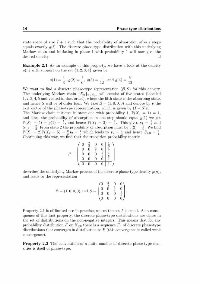
Example 2.1 As an example of this property, we have a look at the densityg(n) with support on the set {1, 2, 3, 4} given by
g(1) =13, g(2) =
16, g(3) =
112
, and g(4) =512
.
We want to find a discrete phase-type representation (β, S) for this density.The underlying Markov chain {Xn}n∈N≥0 will consist of five states (labelled1, 2, 3, 4, 5 and visited in that order), where the fifth state is the absorbing state,and hence S will be of order four. We take β = (1, 0, 0, 0) and denote by s theexit vector of the phase-type representation, which is given by (I − S)e.The Markov chain initiates in state one with probability 1, P(X0 = 1) = 1,and since the probability of absorption in one step should equal g(1) we getP(X1 = 5) = g(1) = 1
3 , and hence P(X1 = 2) = 23 . This gives s1 = 1
3 andS1,2 = 2
3 . From state 2 the probability of absorption must be g(2) = 16 . We find
P(X1 = 2)P(X2 = 5) = 23s2 = 1
6 which leads to s2 = 14 and hence S2,3 = 3
4 .Continuing this way, we find that the transition probability matrix
P =
0 2
3 0 0 13
0 0 34 0 1
40 0 0 5
616
0 0 0 0 10 0 0 0 1
describes the underlying Markov process of the discrete phase-type density g(n),and leads to the representation
β = (1, 0, 0, 0) and S =
0 2
3 0 00 0 3
4 00 0 0 5
60 0 0 0
.
Property 2.1 is of limited use in practise, unless the set I is small. As a conse-quence of this first property, the discrete phase-type distributions are dense inthe set of distributions on the non-negative integers. This means that for anyprobability distribution F on N≥0 there is a sequence Fn of discrete phase-typedistributions that converges in distribution to F (this convergence is called weakconvergence).
Property 2.2 The convolution of a finite number of discrete phase-type den-sities is itself of phase-type.
2.1 Discrete phase-type distributions 15
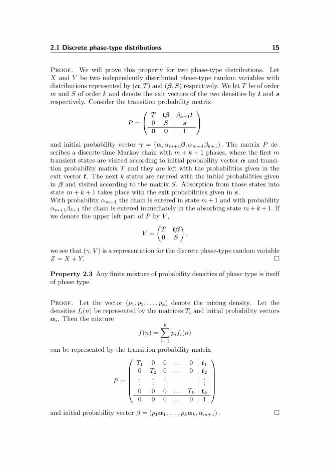
Proof. We will prove this property for two phase-type distributions. LetX and Y be two independently distributed phase-type random variables withdistributions represented by (α, T ) and (β, S) respectively. We let T be of orderm and S of order k and denote the exit vectors of the two densities by t and srespectively. Consider the transition probability matrix
P =
T tβ βk+1t0 S s0 0 1
and initial probability vector γ = (α, αm+1β, αm+1βk+1) . The matrix P de-scribes a discrete-time Markov chain with m + k + 1 phases, where the first mtransient states are visited according to initial probability vector α and transi-tion probability matrix T and they are left with the probabilities given in theexit vector t. The next k states are entered with the initial probabilities givenin β and visited according to the matrix S. Absorption from those states intostate m + k + 1 takes place with the exit probabilities given in s.With probability αm+1 the chain is entered in state m + 1 and with probabilityαm+1βk+1 the chain is entered immediately in the absorbing state m + k + 1. Ifwe denote the upper left part of P by V ,
V =(
T tβ0 S
),
we see that (γ, V ) is a representation for the discrete phase-type random variableZ = X + Y. �
Property 2.3 Any finite mixture of probability densities of phase type is itselfof phase type.
Proof. Let the vector (p1, p2, . . . , pk) denote the mixing density. Let thedensities fi(n) be represented by the matrices Ti and initial probability vectorsαi. Then the mixture
f(n) =k∑
i=1
pifi(n)
can be represented by the transition probability matrix
P =
T1 0 0 . . . 0 t10 T2 0 . . . 0 t2...
......
...0 0 0 . . . Tk tk
0 0 0 . . . 0 1
and initial probability vector β = (p1α1, . . . , pkαk, αm+1) . �

16 Phase-type distributions
For two matrices A and B of size k ×m and p × q respectively, the Kroneckerproduct A⊗B is given by
A⊗B =
a11B . . . a1mB...
. . ....
ak1B . . . akmB
.
Hence A ⊗ B has size kp ×mq. We can use the Kronecker product to expressthe maximum and minimum of two discrete phase-type variables.
Property 2.4 Let X and Y be discrete phase-type distributed with parameters(α, T ) and (β, S) respectively. Then U = min(X, Y ) is discrete phase-typedistributed with parameters (α ⊗ β, T ⊗ S) and V = max(X, Y ) is discretephase-type distributed with parameters
γ = (α⊗ β, βk+1α, αm+1β),
L =
T ⊗ S I ⊗ s t⊗ I0 T 00 0 S
.
Proof. In order to prove that the minimum U is of discrete phase-type we haveto find a Markov chain where the time until absorption has the same distributionas the minimum of X and Y . This minimum is the time until the first of the twounderlying Markov chains of X and Y gets absorbed. We make a new Markovchain that keeps track of the state of both underlying Markov chains of X and Y .The state space of this new Markov chain consists of all combinations of states ofX and Y . Hence, if X has order m and Y has order k we have the new state space{(1, 1), (1, 2), . . . , (1, k), (2, 1), (2, 2), . . . , (2, k), . . . , (m, 1), (m, 2), . . . , (m, k)}.The mk × mk order transition probability matrix corresponding to this newMarkov chain is given by T ⊗ S since each entry tijS gives for a transition inthe Markov chain corresponding to (α, T ) all possible transitions in the Markovchain corresponding to (β, S). The corresponding initial probability vector isgiven by α⊗ β.The maximum V is the time until both underlying Markov chains of X and Yget absorbed. This means that after one of the Markov chains gets absorbed weneed to keep track of the second Markov chain until it too gets absorbed. Hencewe need a new Markov chain with mk + m + k states, where the first mk statesare the same as in the case of the minimum above. Then with the probabilitiesin the exit vector s the Markov chain of Y gets absorbed, and our new Markovchain continues in the states of X. And with the probabilities in the exit vectort the Markov chain of X gets absorbed and our new Markov chain continues inthe states of Y. Hence the matrix L describes the transition probabilities in thenew Markov chain. If one of the Markov chains initiates in the absorbing state

2.1 Discrete phase-type distributions 17
we only have to keep track of the remaining Markov chain. Hence the initialprobability vector corresponding to the matrix L is given by γ. �
The last property is about the N -fold convolution of a discrete phase-type distri-bution, where N is also discrete phase-type distributed. For ease of computationwe will assume in the following that the probability of initiating in the absorbingstate is zero.
Property 2.5 Let Xi ∼ DPH(α, T ) i.i.d. and N ∼ DPH(β, S). Then theN -fold convolution of the Xi,
Z =N∑
i=1
Xi
is again discrete phase-type distributed, with representation (γ, V ) where
γ = (α⊗ β)
and V is the upper left part of the transition probability matrix
P =(
T ⊗ I + (tα)⊗ S t⊗ s0 1
),
where the identity matrix has the same dimension as the matrix S.
Proof. The interpretation of the matrix V = (T ⊗ I + (tα) ⊗ S) is that firstthe transient states of the Markov chain corresponding to the Xi are visitedaccording to the transition probabilities in T . When this Markov chain getsabsorbed with the probabilities given in t, the Markov chain underlying N isvisited according to S. If absorption in this second Markov chain does not takeplace, the first Markov chain will be revisited with initial probabilities given inα. The new system corresponding to V is absorbed when both the first and thesecond Markov chain get absorbed. �
We will make this probabilistic proof more clear with the following example.
Example 2.2 Let Xi ∼ DPH(α, T ) be represented by the following vector andmatrix:
α = (1, 0), T =(
12
13
13
13
)and let N ∼ DPH(β, S) be geometrically distributed with success probabilityp ∈ (0, 1), hence
β = 1, S = (1− p).

18 Phase-type distributions
This leads to the exit vectors t =(
1613
)and s = p. The underlying Markov
chains for the Xi and for N are shown in Figure 2.1:
1 2 313
12
16
13
13
13
1
(I) Underlying Markov chain of Xi
a b
p
1− p 1
(II) Underlying Markov chain of N
Figure 2.1: The Markov chains corresponding to Xi and N .
Using γ = (α⊗β) and V = (T ⊗ I + (tα)⊗S) we get for the representation ofZ:
γ = (1, 0), V =(
12 + 1
6 · (1− p) 13 + 0 · (1− p)
13 + 1
3 · (1− p) 13 + 0 · (1− p)
),v =
(p6p3
).
The interpretation of this N -fold convolution of the Xi is that first states 1 and2 of (I) are visited, and when the absorbing state 3 is reached the Markov chaingiven in (II) is started. With probability (1−p) this Markov chain chooses to gofor another round in (I), and with probability p this Markov chain gets absorbedin state b and then the total system is absorbed. We can think of the Markovchain underlying Z as a combination of (I) and (II), where the states 3 and aare left out, as the probabilities of going from state 1 or 2 through state 3 andstate a back to state 1 are equal to the new probabilities given in the matrix Vof going directly from state 1 or 2 to state 1. Figure 2.2 depicts this Markovchain underlying the random variable Z:
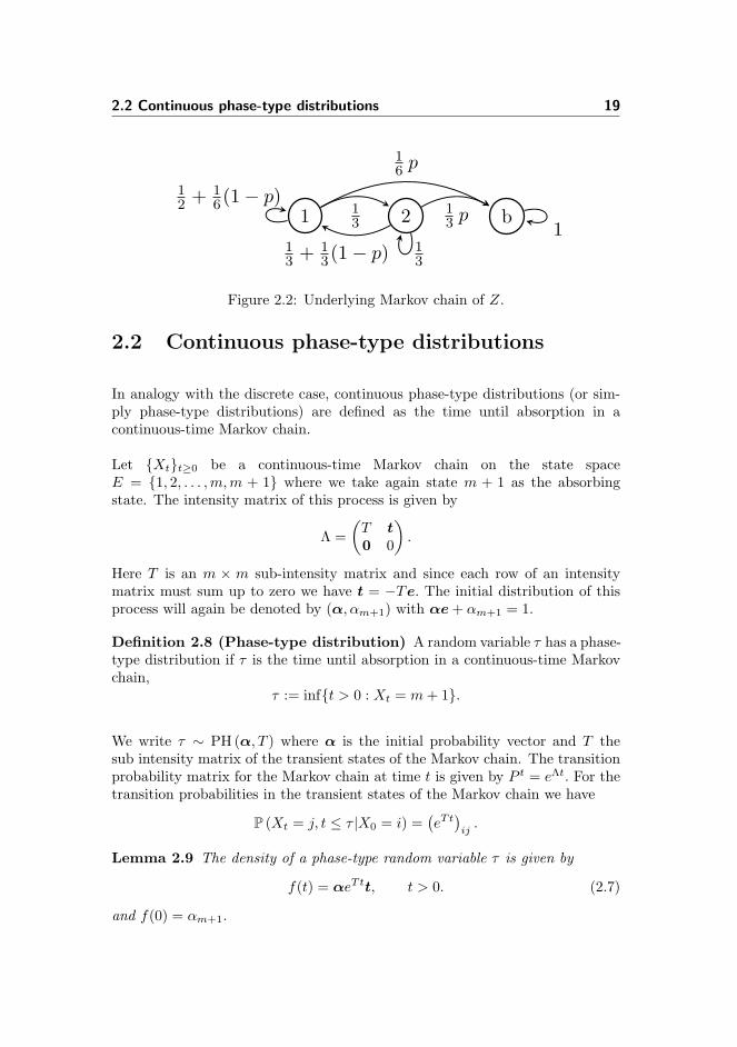
2.2 Continuous phase-type distributions 19
1 2 b13
12 + 1
6(1− p)
16 p
13 p
13
13 + 1
3(1− p)1
Figure 2.2: Underlying Markov chain of Z.
2.2 Continuous phase-type distributions
In analogy with the discrete case, continuous phase-type distributions (or sim-ply phase-type distributions) are defined as the time until absorption in acontinuous-time Markov chain.
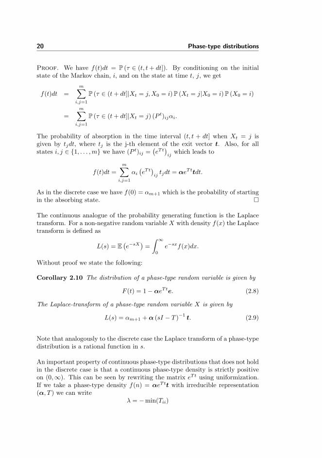
Let {Xt}t≥0 be a continuous-time Markov chain on the state spaceE = {1, 2, . . . ,m, m + 1} where we take again state m + 1 as the absorbingstate. The intensity matrix of this process is given by
Λ =(
T t0 0
).
Here T is an m × m sub-intensity matrix and since each row of an intensitymatrix must sum up to zero we have t = −Te. The initial distribution of thisprocess will again be denoted by (α, αm+1) with αe + αm+1 = 1.
Definition 2.8 (Phase-type distribution) A random variable τ has a phase-type distribution if τ is the time until absorption in a continuous-time Markovchain,
τ := inf{t > 0 : Xt = m + 1}.
We write τ ∼ PH (α, T ) where α is the initial probability vector and T thesub intensity matrix of the transient states of the Markov chain. The transitionprobability matrix for the Markov chain at time t is given by P t = eΛt. For thetransition probabilities in the transient states of the Markov chain we have
P (Xt = j, t ≤ τ |X0 = i) =(eTt)ij
.
Lemma 2.9 The density of a phase-type random variable τ is given by
f(t) = αeTtt, t > 0. (2.7)
and f(0) = αm+1.
20 Phase-type distributions
Proof. We have f(t)dt = P (τ ∈ (t, t + dt]). By conditioning on the initialstate of the Markov chain, i, and on the state at time t, j, we get
f(t)dt =m∑
i,j=1
P (τ ∈ (t + dt]|Xt = j, X0 = i) P (Xt = j|X0 = i) P (X0 = i)
=m∑
i,j=1
P (τ ∈ (t + dt]|Xt = j) (P t)ijαi.
The probability of absorption in the time interval (t, t + dt] when Xt = j isgiven by tjdt, where tj is the j-th element of the exit vector t. Also, for allstates i, j ∈ {1, . . . ,m} we have (P t)ij =
(eTt)ij
which leads to
f(t)dt =m∑
i,j=1
αi
(eTt)ij
tjdt = αeTttdt.
As in the discrete case we have f(0) = αm+1 which is the probability of startingin the absorbing state. �
The continuous analogue of the probability generating function is the Laplacetransform. For a non-negative random variable X with density f(x) the Laplacetransform is defined as
L(s) = E(e−sX
)=∫ ∞
0
e−sxf(x)dx.
Without proof we state the following:
Corollary 2.10 The distribution of a phase-type random variable is given by
F (t) = 1−αeTte. (2.8)
The Laplace-transform of a phase-type random variable X is given by
L(s) = αm+1 + α (sI − T )−1t. (2.9)
Note that analogously to the discrete case the Laplace transform of a phase-typedistribution is a rational function in s.
An important property of continuous phase-type distributions that does not holdin the discrete case is that a continuous phase-type density is strictly positiveon (0,∞). This can be seen by rewriting the matrix eTt using uniformization.If we take a phase-type density f(n) = αeTtt with irreducible representation(α, T ) we can write
λ = −min(Tii)
2.2 Continuous phase-type distributions 21
and T = λ(K − I) where K = I + λ−1T. The matrix K is stochastic, since∑j
Kij =∑
j
Tij
λ+ 1 = 1
and
Kij =Tij
λ= − Tij
minTii≤ 1
Kii =Tii
λ+ 1 = − Tii
minTii+ 1 ≥ 0.
We find for eTt:
eTt = eλ(K−I)t
= e−λt∞∑
i=0
(λt)i
i!Ki
which is a non-negative matrix. If the matrix Ki is irreducible from some ion, (hence the matrix T is irreducible), this matrix will be strictly positive. Ifthis is not the case, there will be states in the underlying Markov chain thatcannot be reached from certain other states. However, the choice of α willmake sure that all states can be reached with positive probability as we havechosen the representation (α, T ) to be irreducible (meaning we left out all thestates that cannot be reached). Hence αeTt is a strictly positive row vectorand multiplying this vector with the non-negative non-empty column vector tensures that αeTtt > 0 for all t > 0.
Example 2.3 If we take a phase-type density with representation
α = (1, 0, 0), T =
−λ λ 00 −λ λ0 0 −λ
and t =
00λ
then we have a continuous phase-type distribution where each phase is visitedan exp(λ) distributed time before the process enters the next phase. Since thereare three transient states this is the sum of three exponential distributions andhence an Erlang-3 distribution. The density of this distribution is given by
f(t) = αeTtt
= (1, 0, 0)
e−λt e−λtλt 12e−λtλ2t2
0 e−λt e−λtλt0 0 e−λt
00λ
= λe−λt (λt)2
2,
which we recognize as the Erlang-3 density.

22 Phase-type distributions
Chapter 3
Matrix-exponentialdistributions
This chapter is about matrix-exponential distributions. They are distribu-tions with a density of the same form as continuous phase-type distributions,f(t) = αeTtt, but they do not necessarily possess the probabilistic interpreta-tion as the time until absorption in a continuous-time finite-state Markov chain.In this chapter we explore some identities and give some examples of matrix-exponential distributions. It serves as a preparation to the next chapter in whichwe will study the discrete analogous of matrix-exponential distributions.A thorough introduction to matrix-exponential distributions is given by As-mussen and O’Cinneide in [4].In Section 3.1 the definition of a matrix-exponential distribution is given, andthe equivalent definition as distributions with a rational Laplace transform isaddressed. In Section 3.2 we give three examples of matrix-exponential distri-butions and explain their relationship to phase-type distributions.

24 Matrix-exponential distributions
3.1 Definition
Definition 3.1 (Matrix-exponential distribution) A random variable Xhas a matrix-exponential distribution if the density of X is of the form
f(t) = αeTtt, t ≥ 0.
Here α and t are a row and column vector of length m and T is an m × mmatrix, all with entries in C.
If we denote the class of matrix-exponential distributions by ME and the classof phase-type distributions by PH we immediately have the relation PH ⊆ ME.In the next section we will show that in fact PH ( MG. The matrix-exponentialdistributions generalize phase-type distributions in the sense that they do notneed to possess the probabilistic interpretation as a distribution of the time untilabsorption in a continuous-time Markov chain. This means that the vector αand matrix T are not necessarily an initial probability vector and sub-intensitymatrix, which allows them to have entries in C. As T is no longer a sub-intensitymatrix, the relation t = −Te does not necessarily hold. Hence the vector tbecomes a parameter, and we write
X ∼ ME(α, T, t)
for a matrix-exponential random variable X.
There is an equivalent definition of the class of matrix-exponential distributions,that says that a random variable X has a matrix-exponential distribution if theLaplace transform L(s) of X is a rational function in s. The connection betweenthe rational Laplace transform and density of a matrix-exponential distributionis made explicit in the following proposition, which is taken from Asmussen &Bladt [3].
Proposition 3.2 The Laplace transform of a matrix-exponential distributioncan be written as
L(s) =b1 + b2s + b3s
2 + . . . + bnsn−1
sn + a1sn−1 + . . . + an−1s + an, (3.1)
for some n ≥ 1 and some constants a1, . . . , an, b1, . . . , bn. From L(0) = 1 itfollows that we have an = b1. The distribution has the following representation
f(t) = αeTtt

3.2 Examples of matrix-exponential distributions 25
where
α = (b1, b2, . . . , bn)
T =
0 1 0 0 0 . . . 0 00 0 1 0 0 . . . 0 0.. .. .. .. .. . . . .. ..0 0 0 0 0 . . . 0 1−an −an−1 −an−2 −an−3 −an−4 . . . −a2 −a1
and
t =
000..01
. (3.2)
Proof. The proof of this proposition can be found in [3] pages 306-310.
If T is an m ×m matrix, the corresponding matrix-exponential distribution issaid to be of order m. If we write L(s) = p(s)
q(s) then d = deg(q) is the degree ofthe matrix-exponential distribution.Note that Proposition 3.2 is of great importance as it gives a method to findan order-d representation of a matrix-exponential density that has a Laplacetransform of degree d.
3.2 Examples of matrix-exponential distributions
In this section we will give three examples of matrix-exponential distributions.Our main aim with these examples is to illustrate that the class of matrix-exponential distributions is strictly larger than the class of phase-type distri-butions and that it is sometimes more convenient to use a matrix-exponentialrepresentation for a distribution because it can be represented with a lower or-der representation (i.e. the matrix T has a lower dimension).To be able to say whether or not a distribution is of phase-type we use the follow-ing Characterization Theorem for phase-type distributions by C.A. O’Cinneide[14].

26 Matrix-exponential distributions
Theorem 3.3 (Characterization of phase-type distributions) A distribu-tion on [0,∞) with rational Laplace-Stieltjes transform is of phase-type if andonly if it is either the point mass at zero, or (a) it has a continuous positivedensity on the positive reals, and (b) its Laplace-Stieltjes transform has a uniquepole of maximal real part.
The proof of this theorem is far from simple and can be found in [14]. Condition(a) of the characterization, stating that a phase-type density is always positiveon (0,∞), has already been addressed in Chapter 2 on page 20. Condition (b)implies that a distribution can only be of phase-type if the sinusoidal effects inthe tail behavior of the density of a phase-type distribution (which cause twoconjugate complex poles in the Laplace-Stieltjes transform) decay at a fasterexponential rate than the dominant effects.
The first example is of a matrix-exponential distribution that does not satisfyCondition (a) and (b) of Theorem 3.3, and hence is not of phase-type.
Example 3.1 A distribution that is genuinely matrix-exponential (hence notof phase-type) is represented by the following density:
f(t) = Ke−λt(1− cos(ωπt)), t ≥ 0
for λ and ω real coefficients and K a scaling coefficient given by
K =λ(λ2 + π2ω2)
π2ω2.
Figure 3.1 shows this density for λ = 1 and ω = 2, which implies K = 1 + 14π2 .
This density is zero whenever t equals 2nω for n ∈ N and therefore violates
Condition (a) of Theorem 3.3. By rewriting this density using the identitycos x = eix+e−ix
2 we find a matrix-exponential representation for this density:
f(t) = Ke−λt(1− cos(ωπt))
= Ke−λt(1−(
eiωπt + e−iωπt
2
))
= Ke−λt − K
2e−t(−iωπ+λ) − K
2e−t(iωπ+λ)
= (1,−1,−1)
e−λt 0 00 e−t(−iωπ+λ) 00 0 e−t(iωπ+λ)
KK2K2
.
3.2 Examples of matrix-exponential distributions 27
1 2 3 4t
0.2
0.4
0.6
0.8
1.0
1.2
f HtL
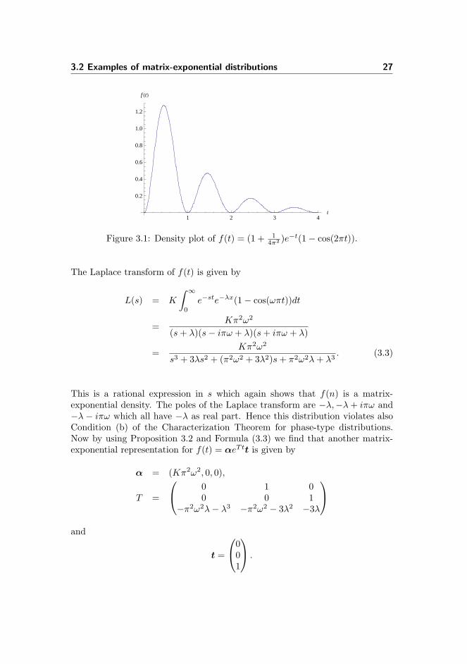
Figure 3.1: Density plot of f(t) = (1 + 14π2 )e−t(1− cos(2πt)).
The Laplace transform of f(t) is given by
L(s) = K
∫ ∞
0
e−ste−λx(1− cos(ωπt))dt
=Kπ2ω2
(s + λ)(s− iπω + λ)(s + iπω + λ)
=Kπ2ω2
s3 + 3λs2 + (π2ω2 + 3λ2)s + π2ω2λ + λ3. (3.3)
This is a rational expression in s which again shows that f(n) is a matrix-exponential density. The poles of the Laplace transform are −λ,−λ + iπω and−λ − iπω which all have −λ as real part. Hence this distribution violates alsoCondition (b) of the Characterization Theorem for phase-type distributions.Now by using Proposition 3.2 and Formula (3.3) we find that another matrix-exponential representation for f(t) = αeTtt is given by
α = (Kπ2ω2, 0, 0),
T =
0 1 00 0 1
−π2ω2λ− λ3 −π2ω2 − 3λ2 −3λ
and
t =
001
.
28 Matrix-exponential distributions
1 2 3 4 5t
0.2
0.4
0.6
0.8
1.0
1.2
1.4
gHtL
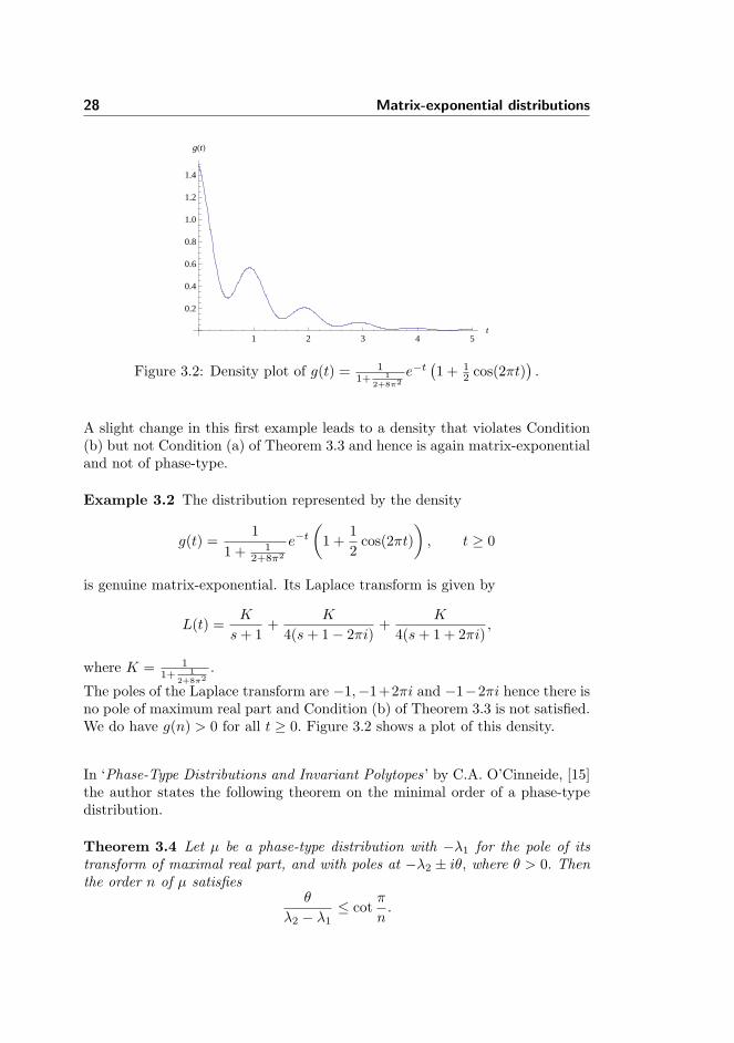
Figure 3.2: Density plot of g(t) = 11+ 1
2+8π2e−t
(1 + 1
2 cos(2πt)).
A slight change in this first example leads to a density that violates Condition(b) but not Condition (a) of Theorem 3.3 and hence is again matrix-exponentialand not of phase-type.
Example 3.2 The distribution represented by the density
g(t) =1
1 + 12+8π2
e−t
(1 +
12
cos(2πt))
, t ≥ 0
is genuine matrix-exponential. Its Laplace transform is given by
L(t) =K
s + 1+
K
4(s + 1− 2πi)+
K
4(s + 1 + 2πi),
where K = 11+ 1
2+8π2.
The poles of the Laplace transform are −1,−1+2πi and −1−2πi hence there isno pole of maximum real part and Condition (b) of Theorem 3.3 is not satisfied.We do have g(n) > 0 for all t ≥ 0. Figure 3.2 shows a plot of this density.
In ‘Phase-Type Distributions and Invariant Polytopes’ by C.A. O’Cinneide, [15]the author states the following theorem on the minimal order of a phase-typedistribution.
Theorem 3.4 Let µ be a phase-type distribution with −λ1 for the pole of itstransform of maximal real part, and with poles at −λ2 ± iθ, where θ > 0. Thenthe order n of µ satisfies
θ
λ2 − λ1≤ cot
π
n.

3.2 Examples of matrix-exponential distributions 29
Using the fact that tanx ≥ x, for 0 ≤ x ≤ 12π, this implies that
n ≥ πθ
λ2 − λ1. (3.4)
Using this theorem we can give an example of a distribution that has a lowerorder when represented as a matrix-exponential density than when representedas a phase-type density.
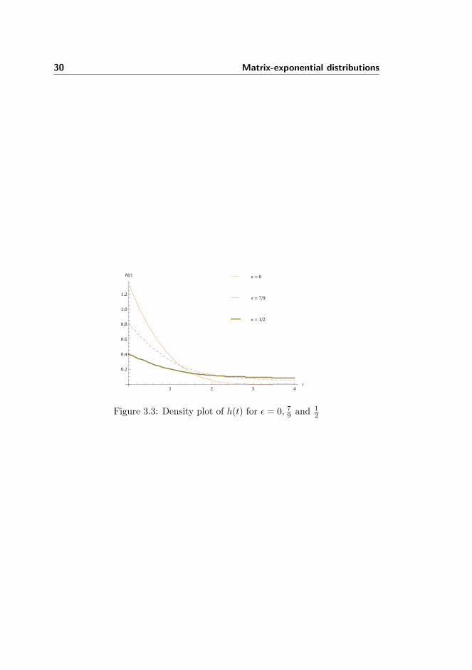
Example 3.3 This is an elaboration of an example in [15] on page 524. Thedensity
h(t) =
(1
12 + 1
1−ε
)(e−(1−ε)t + e−t cos t
), t ≥ 0
for 0 < ε < 1 has Laplace transform
L(s) =2(−1 + ε)(−3 + ε− 4s + εs− 2s2)(−3 + ε)(−1 + ε− s)(2 + 2s + s2)
.
The denominator of L(s) is of degree three and hence h(t) has a matrix-exponentialrepresentation of order three, which can again be found by using Proposition3.2. The poles of the Laplace transform are −1 − i,−1 + i and − 1 + ε. Thusby Theorem 3.4 and Inequality (3.4) we have for the order m of the phase-typerepresentation for h(t) that
m ≥ π
ε.
Hence we have a phase-type density of degree three but with arbitrarily largeorder. Note that for ε = 0 this density is not of phase-type since it then doesn’thave a unique pole of maximum real part. Figure 3.3 shows the density plot ofh(t) for ε = 0, 7/9 and 1/2.
In this chapter we have shown that the class of matrix-exponential distributionsis strictly larger than the class of phase-type distributions. We have seen thatthere are phase-type distributions that have a larger order than their degree.In the next chapter we will explore the relation between matrix-geometric dis-tributions, which are the discrete analogous of matrix-exponential distributionsand discrete phase-type distributions.
30 Matrix-exponential distributions
1 2 3 4t
0.2
0.4
0.6
0.8
1.0
1.2
hHtL
Ε = 1�2
Ε = 7�9
Ε = 0
Figure 3.3: Density plot of h(t) for ε = 0, 79 and 1
2

Chapter 4
Matrix-geometric distributions
This chapter is about the class of matrix-geometric distributions (MG). Theyare distributions on the non-negative integers with a density of the same formas discrete phase-type distributions,
f(n) = αTn−1t.
However, matrix-geometric distributions do not necessarily posses the proba-bilistic interpretation as the time until absorption in a discrete-time Markovchain. They can equivalently be defined as distributions with a rational proba-bility generating function.The main question of this thesis, to be answered in this chapter, is how matrix-geometric distributions relate to discrete phase-type distributions. We will showthat
DPH ( MG
and that there is possible order reduction by taking the matrix-geometric re-presentation for a discrete phase-type distribution.Matrix-geometric distributions are mentioned by Asmussen and O’Cinneide in[4] as the discrete equivalent of matrix-exponential distributions, but no explicitexample of such a distribution is given. They are used by Akar in [1] to studythe queue lengths and waiting times of a discrete time queueing system, but noexplicit examples are given in this article either. Sengupta [17] shows a class of

32 Matrix-geometric distributions
distributions that are obviously in MG, but by the use of a transformation heshows that they are actually in DPH.
In Section 4.1 matrix-geometric distributions are defined. In Section 4.2 weshow that there exist distributions that are genuinely matrix-geometric, hencenot of discrete phase-type, by the use of the Characterization Theorem of dis-crete phase-type distributions stated by O’Cinneide in [14]. In Section 4.3 wewill show that there exist phase-type distributions that have a lower degree,and hence lower order matrix-geometric representation, than the order of theirdiscrete phase-type representation. Finally, in Section 4.4 we will revisit someproperties of discrete phase-type distributions and show that they also hold forthe class MG, by proving them analytically.
4.1 Definition
Definition 4.1 (Matrix-geometric distribution) A random variable X hasa matrix-geometric distribution if the density of X is of the form
f(n) = αTn−1t, n ∈ N
where α and t are a row and column vector of length m and T is an m × mmatrix with entries in C.
We have to make a note about the support of these distributions. Matrix-geometric distributions have support on the non-negative integers, and thematrix-geometric density is actually a mixture of the above density definedon n ∈ N and the point mass at zero. For convenience we will assume in thischapter that f(0) = 0.
The following proposition shows that we can equivalently define matrix-geometricdistributions as distributions that have a rational probability generating func-tion. It is the discrete equivalent of Proposition 3.2.
Proposition 4.2 The probability generating function of a matrix-geometric dis-tribution can be written as
H(z) =bnz + bn−1z
2 + . . . + b2zn−1 + b1z
n
1 + a1z + a2z2 + . . . + an−1zn−1 + anzn, (4.1)
for some n ≥ 1 and constants a1, . . . , an, b1, . . . , bn in R. The correspondingdensity is given by
f(n) = αTn−1t

4.1 Definition 33
where
α = (1, 0, . . . , 0),
T =
−a1 0 0 0 0 . . . 0 1−an 0 0 0 0 . . . 0 0−an−1 1 0 0 0 . . . 0 0
......
......
......
......
−a2 0 0 0 0 . . . 1 0
and
t =
bn
b1
b2
...bn−1
. (4.2)
We call this the canonical form of the matrix-geometric density.
Proof. From Equation (2.9) and Proposition 3.2 we know that we have thefollowing formula for the Laplace transform of a matrix-exponential distribution:
L(s) = α (sI − T )−1t =
b1 + b2s + b3s2 + . . . + bnsn−1
sn + a1sn−1 + . . . + an−1s + an.
In Proposition 3.2 the corresponding vectors α and t and a matrix T are given,using the coefficients of the Laplace transform.
The probability generating function of a matrix-geometric distribution is givenby
H(z) = αz (I − zT )−1t.
This formula is equal to the matrix formula of the Laplace transform if s isreplaced by 1/z, which leads to the following fractional form of the probabilitygenerating function:
H(z) = L(1z) =
b1 + b2z + b3
z2 + . . . + bn
zn−1
1zn + a1
zn−1 + . . . + an−1z + an
=bnz + bn−1z
2 + . . . + b2zn−1 + b1z
n
1 + a1z + a2z2 + . . . + an−1zn−1 + anzn.
The corresponding vectors α and t and a matrix T are hence the same as inProposition 3.2 in Formula (3.2). To obtain the canonical form for a matrix-geometric density given in Formula (4.2) we take the transpose of α, t and Tand rename the states to obtain α = (1, 0, . . . , 0). �

34 Matrix-geometric distributions
As in the continuous case, the order of a matrix-geometric distribution is said tobe m if T is an m×m matrix. If we write H(z) = p(z)
q(z) , the degree of a matrix-geometric distribution is given by n = deg(p). It follows from Proposition 4.2that for a matrix-geometric distribution we can always find a representationthat has the same order as the degree of the distribution.
If a random variable X has a matrix-geometric distribution with parametersα, T and t we write
X ∼ MG(α, T, t) .
Although the relation Te+t = e does not necessarily holds, it is always possibleto find a representation that does satisfies this relation. For a non-singularmatrix M we can write for the density f(n) of X:
f(n) = αTn−1t
= αMM−1Tn−1MM−1t
= αM(M−1TM)n−1M−1t.
For this density we now want the relation
M−1TMe + M−1t = e
to hold, which can found to be true when M satisfies the relation
Me = (I − T )−1t.
4.2 Existence of genuine matrix-geometric dis-tributions
From the definition of matrix-geometric distributions it is immediately clearthat the relation
DPH ⊆ MG
must hold. The question arises though whether or not DPH ( MG ? In thecontinuous case it was easy to find an example of a distribution that is matrix-exponential but not of phase-type, as phase-type distributions can never be zeroon (0,∞). But this is not the case for discrete phase-type distributions, as theycan have a periodicity which allows them to be zero with a certain period d.
In ’Characterization of phase-type distributions’ by C.A. O’Cinneide,[14], thefollowing characterization of discrete phase-type distributions is given.
4.2 Existence of genuine matrix-geometric distributions 35
Theorem 4.3 (Characterization of discrete phase-type distributions)A probability measure µ on {0, 1, . . .} with rational generating function is ofphase type if and only if for some positive integer ω each of the generatingfunctions
Hµ,k(z) =∞∑
n=0
µ(ωn + k)zn, (4.3)
for k = 0, 1, . . . , ω − 1, is either a polynomial or has a unique pole of minimalabsolute value.
The proof of this theorem can be found in [14], pages 49-56. Here, we will givean outline of the proof.
Necessity. Let µ be discrete phase-type. Then either µ is the point mass atzero, for which Theorem 4.3 holds with ω = 1 or µ has an irreducible repre-sentation (α, T ) of positive order. In the latter case, we let {Xn}n∈N be theMarkov chain corresponding to this representation. Let ω be the least com-mon multiple of the periods of all the periodic classes of the chain X. Letτ be the time until absorption of the Markov chain, hence τ has distributionµ. If P (τ = k mod ω) = 0 then Hµ,k(z) is identically zero and hence a poly-nomial. If however P (τ = k mod ω) > 0 we can define a new Markov chain{Yn} = {Xk+ωn} which given that τ = k mod ω is an absorbing Markov chainwith one absorbing state and possibly fewer transient states than our originalchain since we can leave out the states than can never be reached.If we denote by αk the initial distribution of Y0 and by Sk the transition pro-bability matrix of its transient states we have that (αk, Sk) is an irreduciblerepresentation of the conditional distribution of τ−k
ω given τ = k mod ω. By thedefinition of ω, the transition matrix Sk has no periodic states. If we call thisdistribution µk we have that Hµk
(z) = Hµ,k(z)Hµ,k(1) for all z.
In order to prove that Hµ,k has a unique pole of minimal value it suffices nowto prove that Hµk
(z) has one, since Hµ,k(z) is just a positive multiple of Hµk(z)
and their poles are equal. Let ζk denote the unique eigenvalue of Sk of largestabsolute value, whose existence is assured by the Perron-Frobenius theorem (seee.g. [8], page 240). The uniqueness of ζk is a consequence of Sk being aperi-odic which implies that it cannot have non-real eigenvalues of maximal modulus(see Thm. 3.3.1 in [11]). Since Sk is a transition probability matrix, ζk is lessthan one. As the poles of Hµk
(z) are the reciprocals of the eigenvalues of Sk, itfollows 1
ζkis the unique pole of minimal value of Hµk
(z) and hence of Hµ,k(z).The other poles of Hµ,k(z) will have greater absolute value, which concludes theproof of necessity.

36 Matrix-geometric distributions
Sufficiency. Let µ be a probability measure on {0, 1, . . .} with rational gen-erating function and with each of the generating functions Hµ,k(z) either apolynomial or with a unique pole of minimal absolute value. In [14] it is proventhat a probability measure with rational generating function with a unique poleof minimal absolute value is of discrete phase-type. The proof of this statementmakes use of invariant polytopes and is beyond the scope of this thesis.However, this statement is the crux of the proof for the sufficiency of the condi-tion to be of discrete phase-type. We can finish the proof with the following ar-gument. The probability measure µk with generating function Hµk
(z) = Hµ,k(z)Hµ,k(1)
is of discrete phase-type as Hµk(z) has a unique pole of minimal absolute value.
Let τk be a random variable with distribution µk for k = 0, 1, . . . , ω − 1. Thenωτk is again of discrete phase-type, as we can modify the state space such thatfrom every original state there is a deterministic series of ω − 1 transitionsthrough ω − 1 new states after which again an original state is reached. As aconstant c can be modelled as a phase-type distribution with transition matrixof dimension c with Ti,i+1 = 1 for all states i we have that also ωτk+k is discretephase-type distributed. Now µ is a mixture of the distributions µk for ωτk + kin proportions of Hµ,k(1) for k = {0, 1, . . . , ω − 1}. Hence µ is a finite mixtureof discrete phase-type distributions and is so itself of discrete phase-type, whichcompletes the proof for sufficiency. �
Based on this characterization of discrete phase-type distributions we can provethe following theorem:
Theorem 4.4 The class of matrix-geometric distributions is strictly larger thanthe class of discrete phase-type distributions.
Proof. We prove this theorem by giving an example of a matrix-geometricdistribution that does not meet the necessary condition stated in Theorem 4.3to be of discrete phase-type. We have a look at a matrix-geometric distributionwith density
g(n) = Kpn−1(1 + cos(
√2(n− 1))
), n ∈ N (4.4)
for K a normalizing constant and p ∈ (0, 1). We can rewrite this density to getit into matrix-geometric form:
g(n) = Kpn−1(1 + cos
(√2(n− 1)
))= Kpn−1
(1 +
12ei√
2(n−1) +12e−i
√2(n−1)
)
4.2 Existence of genuine matrix-geometric distributions 37
= Kpn−1 +12Kpn−1ei
√2(n−1) +
12Kpn−1e−i
√2(n−1)
= Kpn−1 +12K(pei
√2)n−1
+12K(pe−i
√2)n−1
= (1, 1, 1)
p 0 00 pei
√2 0
0 0 pe−i√
2
n−1 K12K12K
. (4.5)
We write as usual g(n) = αTn−1t. According to Theorem 4.3 a necessary condi-tion for this density to be of discrete phase-type is that the probability genera-ting functions Hg,k(z) =
∑∞n=0 g(ωn+k)zn for some ω ∈ N are either a polyno-
mial or have a unique pole of minimal absolute value for all k = 0, 1, . . . , ω − 1.For k = 1, 2, . . . , ω − 1 these generating functions are given by
Hg,k(z) =∞∑
n=0
g(ωn + k)zn
=∞∑
n=0
αTωn+k−1tzn
= α∞∑
n=0
TωnT k−1znt
= α
( ∞∑n=0
(zTω)n
)T k−1t
= α (I − zTω)−1T k−1t. (4.6)
For k = 0 we get
Hg,0(z) =∞∑
n=0
g(ωn)zn
= g(0) +∞∑
n=1
αTωn−1tzn
= 0 + α∞∑
n=1
Tωn−1−ω+1Tω−1znt
= αz
( ∞∑n=1
(zTω)n−1
)Tω−1t
= αz (I − zTω)−1Tω−1t. (4.7)
We see that the zeros of the denominator of these generating functions aregiven by the reciprocals of the eigenvalues of the matrix Tω. We have to checkfor Formula (4.7) that none of these zeros cancel. We can use the representation

38 Matrix-geometric distributions
of g(n) in (4.5) to find
αz (I − zTω)−1Tω−1t = K
zpω−1
1− zpω+
12K
zpei√
2(ω−1)
1− zpei√
2ω+
12K
zpe−i√
2(ω−1)
1− zpe−i√
2ω.
Hence the poles of both (4.6) and (4.7) are given by p−ω, p−ωe−i√
2ω and p−ωei√
2ω,which are the reciprocals of the eigenvalues of the matrix
Tω =
pω 0 00 pωei
√2ω 0
0 0 pωe−i√
2ω
and which are not a zero of the numerator of Hg,0(z). These poles all have equalabsolute value p−ω. The only possibility for Hg,k(z) to have a unique pole ofmaximum absolute value is for ω = k
√2π because then ei
√2ω = ek2πi = 1 and
Tω will have eigenvalue pk√
2π with multiplicity three. However, according toTheorem 4.3, ω must be chosen in N, which proves that it is not possible forHg,k(z) to have a unique pole of minimal absolute value.Finally, we know that Hg,k(z) is not the zero polynomial since g(n) is positivefor all n ∈ N, which is a consequence of (1 + cos(
√2(n − 1)) not having a zero
in the integer numbers.We can conclude that the distribution represented by g(n) is genuinely matrix-geometric and that the class of matrix-geometric distributions is strictly largerthan the class of discrete phase-type distributions. �
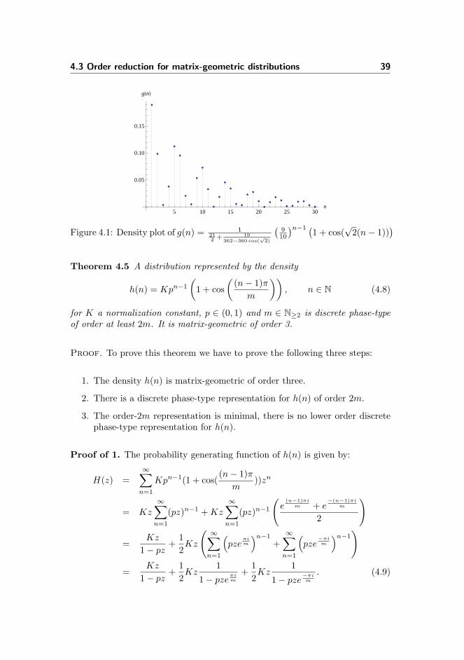
Example 4.1 The density
g(n) =1
212 + 19
362−360 cos(√
2)
(910
)n−1 (1 + cos(
√2(n− 1))
)is genuinely matrix-geometric. Figure 4.1 shows the density plot of g(n).
4.3 Order reduction for matrix-geometric distri-butions
Example 3.3 of Chapter 3 showed a class of phase-type distributions that havedegree three, and hence matrix-exponential representation of order three, butthat need m ≥ π
ε phases for their phase-type representation, which hence can bearbitrarily large for ε ↓ 0. In this section we will show that such order reductioncan also take place when going from a discrete phase-type representation to amatrix-geometric representation.
4.3 Order reduction for matrix-geometric distributions 39
5 10 15 20 25 30n
0.05
0.10
0.15
gHnL
Figure 4.1: Density plot of g(n) = 1212 + 19
362−360 cos(√
2)
(910
)n−1 (1 + cos(√
2(n− 1)))
Theorem 4.5 A distribution represented by the density
h(n) = Kpn−1
(1 + cos
((n− 1)π
m
)), n ∈ N (4.8)
for K a normalization constant, p ∈ (0, 1) and m ∈ N≥2 is discrete phase-typeof order at least 2m. It is matrix-geometric of order 3.
Proof. To prove this theorem we have to prove the following three steps:
1. The density h(n) is matrix-geometric of order three.
2. There is a discrete phase-type representation for h(n) of order 2m.
3. The order-2m representation is minimal, there is no lower order discretephase-type representation for h(n).
Proof of 1. The probability generating function of h(n) is given by:
H(z) =∞∑
n=1
Kpn−1(1 + cos((n− 1)π
m))zn
= Kz
∞∑n=1
(pz)n−1 + Kz
∞∑n=1
(pz)n−1
(e
(n−1)πim + e
−(n−1)πim
2
)
=Kz
1− pz+
12Kz
( ∞∑n=1
(pze
πim
)n−1
+∞∑
n=1
(pze
−πim
)n−1)
=Kz
1− pz+
12Kz
11− pze
πim
+12Kz
1
1− pze−πim
. (4.9)

40 Matrix-geometric distributions
This is a rational function in z of degree three. Hence h(n) has an order threematrix-geometric representation (see also Example 4.2).
Proof of 2. The density h(n) is zero for n = m + 1, 3m + 1, 5m + 1, . . .. Henceit has a period of 2m and the following discrete phase-type representation is areasonable candidate to represent h(n):
h(n) = αTn−1t (4.10)
with
α = (1, 0, . . . , 0)
T =
0 t1,2 0 0 0 . . . . . . 00 0 t2,3 0 0 . . . . . . 0...
......
. . ....
......
...0 0 0 0 tm,m+1 . . . . . . 00 0 0 0 0 tm+1,m+2 . . . 0...
......
......
.... . .
...0 0 0 0 0 . . . . . . t2m−1,2m
t2m,1 0 0 0 0 . . . . . . 0
and
t =
1− t1,2
1− t2,3
...1− tm,m+1
1− tm+1,m+2
...1− t2m−1,2m
1− t2m,1
. (4.11)
By equating the first 2m values of h(n) and h(n) we can solve for all the pa-rameters {t1,2, t2,3, . . . , t2m−1,2m, t2m,1} in representation (4.11). We have
h(1) = αt = 1− t1,2
h(2) = αT t = t1,2(1− t2,3)...
h(m) = αTm−1t = t1,2t2,3 . . . tm−1,m(1− tm,m+1)h(m + 1) = αTmt = t1,2t2,3 . . . tm,m+1(1− tm+1,m+2)
...h(2m) = αT 2m−1t = t1,2t2,3 . . . t2m−1,2m(1− t2m,1). (4.12)

4.3 Order reduction for matrix-geometric distributions 41
This system of equations has a unique solution, as the equations can be solvedrecursively. We find
t1,2 = 1− h(1)
t2,3 = 1− h(2)1− h(1)
...
tm+1,m+2 = 1− h(m + 1)1− h(1)− . . .− h(m)
...
t2m,1 = 1− h(2m)1− h(1)− . . .− h(2m− 1)
.
Note that ti,j ∈ (0, 1) for (i, j) 6= (m + 1,m + 2) since h(i) ∈ (0, 1) fori ∈ {1, . . . ,m, m + 2, . . . , 2m} and
h(1) + . . . + h(i) < 1 ⇒h(i) < 1− h(1)− . . .− h(i− 1) ⇒
h(i)1− h(1)− . . .− h(i− 1)
< 1 ⇒
ti,j = 1− h(i)1− h(1)− . . .− h(i− 1)
> 0.
That ti,j < 1 follows directly from the equations in (4.12). From h(m + 1) = 0we deduce that tm+1,m+2 = 1 which implies that absorption is not possible fromstate m + 1 and we will indeed get h(m + 1 mod 2m) = 0.
We now have two densities h(n) and h(n) that agree on n = 1, . . . , 2m. Itremains to prove that h(n) = h(n) for all n ∈ N. We will do this inductively, byfirst proving that
h(2m + 1) = h(2m + 1) (4.13)
and then, assuming h(s) = h(s) for s ≤ S ∈ N, by showing that
h(s + 1)h(s)
=h(s + 1)
h(s)(4.14)
for all s ∈ N from which h(s + 1) = h(s + 1) follows.
We have h(2m + 1) = 2Kp2m. For the scaling constant K the following formulacan be found by summing separately the terms of h(n) that have the same value

42 Matrix-geometric distributions
of cos (n−1)πm :
1K
=∞∑
n=1
pn−1(1 + cos(n− 1)π
m)
=2m−1∑j=0
pj
1− p2m(1 + cos
jπ
m).
In order to compute h(2m + 1) we need to know what the general form of h(n)is. Let s ∈ N be given by
s = d + ξ · 2m (4.15)
where 1 ≤ d ≤ 2m and ξ ∈ N. The general form of h(s) can be deduced fromthe structure of the matrix T and is given by
h(s) = αT s−1t = (1− td,d+1)tξ+11,2 tξ+1
2,3 . . . tξd,d+1 . . . tξ2m−1,2mtξ2m,1 (4.16)
Now we find
h(2m + 1) = αT 2mt
= (1− t1,2)t1,2t2,3 · · · t2m,1
= h(1)(1− h(1))1− h(1)− h(2)
1− h(1)· · · 1− h(1)− h(2)− . . .− h(2m)
1− h(1)− . . .− h(2m− 1)= −h(1)(−1 + h(1) + . . . h(2m))
= −2K(−1 + K2m−1∑j=0
pj(1 + cosjπ
m))
= 2K − 2K2(1K
(1− p2m))
= 2Kp2m
which is indeed equal to h(2m+1) and hence (4.13) is proven. For the inductionstep we get
h(s + 1)h(s)
=Kpd+k·2m(1 + cos d+k·2mπ
m )Kpd−1+k·2m(1 + cos d−1+k·2mπ
m )= p
1 + cos dπm
1 + cos (d−1)πm

4.3 Order reduction for matrix-geometric distributions 43
whereas
h(s + 1)h(s)
=1− td+1,d+2
1− td,d+1td,d+1
=1−
(1−
∑d+1i=1 h(i)
1−∑d
i=1 h(i)
)1−
(1−
∑di=1 h(i)
1−∑d−1
i=1 h(i)
) 1−∑d
i=1 h(i)
1−∑d−1
i=1 h(i)
=1−
∑di=1 h(i)− (1−
∑d+1i=1 h(i))
1−∑d−1
i=1 h(i)− (1−∑d
i=1 h(i))
=∑d+1
i=1 h(i)−∑d
i=1 h(i)∑di=1 h(i)−
∑d−1i=1 h(i)
=h(d + 1)
h(d)= p
1 + cos dπm
1 + cos (d−1)πm
.
Hence (4.14) is proven and this completes the proof of Step 2. We can concludethat our reasonable candidate h(n) is indeed an order-2m discrete phase-typerepresentation for the density h(n).
Proof of 3. We want to prove that there is no discrete phase-type representa-tion for h(n) of an order lower than 2m.Suppose h(n) has a discrete phase-type representation (β, S) that is of orderd < 2m. Since h(m + 1) = 0 we know that there must be at least one en-try in the vector with exit probabilities s which is zero, say si = 0 for somei ∈ {1, . . . , d}. Let d be the period of the matrix S. As S has order d, we knowthat d ≤ d. We also know that d > 1 because if S has no period then βSn−1swill be strictly positive for all n > d and (β, S) is certainly no representationfor h(n).The periodicity d implies that for 1 ≤ j ≤ d− 1
h(j) = cκh(j + κd) (4.17)
for κ ∈ N and a positive constant c with c < 1. As h(m + 1) = 0, (4.17) impliesthat h(m + 1 + d) = 0. But this is a contradiction, as m + 1 + d < 3m + 1and h(n) is not zero between m + 1 and 3m + 1. Hence (β, S) cannot be adiscrete phase-type representation for h(n) and we can conclude that a discretephase-type representation for h(n) must be at least of order 2m. �
Example 4.2 We take p = 910 and m = 2 in (4.8) which leads to the following
density:
f(n) =1811910
(910
)n−1(1 + cos
((n− 1)π
2
)). (4.18)

44 Matrix-geometric distributions
Figure 4.2 shows the density plot of f(n).
The probability generating function of f(n) is given by
H(z) =181955z − 1629
191000z2 + 14661191000z3
1− 910z + 81
100z2 − 7291000z3
,
which leads to the following matrix-geometric representation for f(n) by the useof Proposition 4.2:
f(n) = αTn−1t
with
α = (1, 0, 0)
T =
910 0 17291000 0 0− 81
100 1 0
and
t =
181955
14661191000
− 162919100
.
By solving the system of equations in (4.12) we can find the following discretephase-type representation of order 4 for f(n) :
α = (1, 0, 0, 0)
T =
0 774
955 0 00 0 1539
1720 00 0 0 1
17191900 0 0 0
and
t =
1819551811720
01811900
.

4.4 Properties of matrix-geometric distributions 45
5 10 15 20 25 30 35n
0.05
0.10
0.15
f HnL
Figure 4.2: Density plot of f(n) = 1811910
(910
)n−1(1 + cos
((n−1)π
2
)).
4.4 Properties of matrix-geometric distributions
For the sake of completeness we will revisit in this section some of the propertiesfor discrete phase-type distributions given in Section 2.1. We will show thatthese properties also hold for the class of matrix-geometric distributions, bygiving an analytic proof for them based on probability generating functions ordistribution functions. The first property, stating that every probability densityon a finite number of positive integers is of discrete phase-type, can clearly beextended to matrix-geometric densities, as the former are a subset of the latter.Hence we start with the equivalence of Property 2.2.
Property 4.1 The convolution of a finite number of matrix-geometric densitiesis itself matrix-geometric.
Proof. We will prove this property for two matrix-geometric densities. Let Xand Y be two independent matrix-geometric random variables with distributionsrepresented by (α, T, t) and (β, S, s) respectively. We let T be of order m andS of order k. Consider the matrix
V =(
T tβ0 S
)and vectors
γ = (α, αm+1β, αm+1βk+1) and v =(
βk+1ts
).
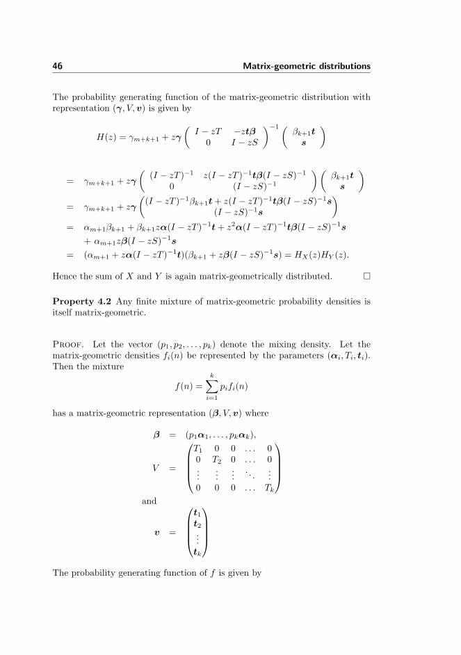
46 Matrix-geometric distributions
The probability generating function of the matrix-geometric distribution withrepresentation (γ, V, v) is given by
H(z) = γm+k+1 + zγ
(I − zT −ztβ
0 I − zS
)−1(βk+1t
s
)
= γm+k+1 + zγ
((I − zT )−1 z(I − zT )−1tβ(I − zS)−1
0 (I − zS)−1
)(βk+1t
s
)= γm+k+1 + zγ
((I − zT )−1βk+1t + z(I − zT )−1tβ(I − zS)−1s
(I − zS)−1s
)= αm+1βk+1 + βk+1zα(I − zT )−1t + z2α(I − zT )−1tβ(I − zS)−1s
+ αm+1zβ(I − zS)−1s
= (αm+1 + zα(I − zT )−1t)(βk+1 + zβ(I − zS)−1s) = HX(z)HY (z).
Hence the sum of X and Y is again matrix-geometrically distributed. �
Property 4.2 Any finite mixture of matrix-geometric probability densities isitself matrix-geometric.
Proof. Let the vector (p1, p2, . . . , pk) denote the mixing density. Let thematrix-geometric densities fi(n) be represented by the parameters (αi, Ti, ti).Then the mixture
f(n) =k∑
i=1
pifi(n)
has a matrix-geometric representation (β, V, v) where
β = (p1α1, . . . , pkαk),
V =
T1 0 0 . . . 00 T2 0 . . . 0...
......
. . ....
0 0 0 . . . Tk
and
v =
t1t2...tk
The probability generating function of f is given by
4.4 Properties of matrix-geometric distributions 47
Hf (z) = zβ(I − zV )−1v
= p1zα1(I − zT1)−1t1 + . . . + pkzαk(I − zTk)tk
= p1Hf1(z) + . . . pkHfk(z).
�
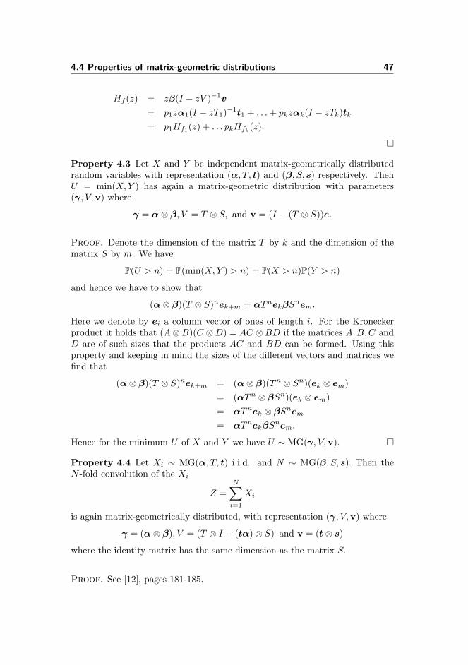
Property 4.3 Let X and Y be independent matrix-geometrically distributedrandom variables with representation (α, T, t) and (β, S, s) respectively. ThenU = min(X, Y ) has again a matrix-geometric distribution with parameters(γ, V,v) where
γ = α⊗ β, V = T ⊗ S, and v = (I − (T ⊗ S))e.
Proof. Denote the dimension of the matrix T by k and the dimension of thematrix S by m. We have
P(U > n) = P(min(X, Y ) > n) = P(X > n)P(Y > n)
and hence we have to show that
(α⊗ β)(T ⊗ S)nek+m = αTnekβSnem.
Here we denote by ei a column vector of ones of length i. For the Kroneckerproduct it holds that (A⊗B)(C ⊗D) = AC ⊗BD if the matrices A,B,C andD are of such sizes that the products AC and BD can be formed. Using thisproperty and keeping in mind the sizes of the different vectors and matrices wefind that
(α⊗ β)(T ⊗ S)nek+m = (α⊗ β)(Tn ⊗ Sn)(ek ⊗ em)= (αTn ⊗ βSn)(ek ⊗ em)= αTnek ⊗ βSnem
= αTnekβSnem.
Hence for the minimum U of X and Y we have U ∼ MG(γ, V,v). �
Property 4.4 Let Xi ∼ MG(α, T, t) i.i.d. and N ∼ MG(β, S, s). Then theN -fold convolution of the Xi
Z =N∑
i=1
Xi
is again matrix-geometrically distributed, with representation (γ, V,v) where
γ = (α⊗ β), V = (T ⊗ I + (tα)⊗ S) and v = (t⊗ s)
where the identity matrix has the same dimension as the matrix S.
Proof. See [12], pages 181-185.
48 Matrix-geometric distributions
Bibliography
[1] N. Akar. A matrix-analytical method for the discrete-time Lindley equationusing the generalized Schur decomposition. In SMCTOOLS’06, October2006.
[2] S. Asmussen. Applied Probability and Queues, volume 51 of Applicationsof Mathematics. Springer, 2nd edition, 2003.
[3] S. Asmussen and M. Bladt. Renewal theory and queueing algorithms formatrix-exponential distributions. In A. Alfa and S.R. Chakravarthy, edi-tors, Matrix-analytic Methods in Stochastic Models, pages 313–341. 1997.
[4] S. Asmussen and C.A. O’Cinneide. Matrix-exponential distributions. En-cyclopedia of Statistical Sciences, 2006.
[5] S. Asmussen and M. Olsson. Phase-type distributions (Update). Encyclo-pedia of Statistical Sciences Update, 2, 1998.
[6] M. Bladt and B.F. Nielsen. Lecture notes on phase-type distributions, 2008.
[7] M. Bladt and B.F. Nielsen. Multivariate matrix-exponential distributions.Submitted, 2008.
[8] G.R. Grimmett and D.R. Stirzaker. Probability and Random Processes.Oxford University Press, 3rd edition, 2001.
[9] V.G. Kulkarni. A new class of multivariate phase type distributions. Op-erations Research, 37(1):151–158, 1989.
[10] G. Latouche and V. Ramaswami. Introduction to Matrix Analytic Meth-ods in Stochastic Modelling. ASA-SIAM Series on Statistics and AppliedProbability. ASA-SIAM, 1999.

50 BIBLIOGRAPHY
[11] H. Minc. Nonnegative Matrices. John Wiley and Sons, 1998.
[12] M.F. Neuts. Probability distributions of phase type. In Liber AmicorumProfessor Emeritus H. Florin, pages 173–206. Department of Mathematics,University of Louvain, Belgium, 1975.
[13] M.F. Neuts. Matrix-Geometric Solutions in Stochastic Models: An Algo-rithmic Approach. Johns Hopkins series in Mathematical sciences; 2. TheJohns Hopkins University Press, Baltimore, 1981.
[14] C.A. O’Cinneide. Characterization of phase-type distributions. StochasticModels, 6(1):1–57, 1990.
[15] C.A. O’Cinneide. Phase-type distributions and invariant polytopes. Ad-vances in Applied Probability, 23(3):515–535, 1991.
[16] E. Seneta. Non-negative Matrices and Markov Chains. Springer Series inStatistics. Springer-Verlag, 2nd edition, 1981.
[17] B. Sengupta. Phase-type representations for matrix-geometric solutions.Stochastic Models, 6(1):163–167, 1990.